Embed Size (px)
Citation preview

Numerical analysis
of partial differential equations
arising in finance
Version of Jan. 15, 20181
J. Frederic Bonnans 2
1Lecture notes of the 2017-2018 course given in the Master 2 ”Probabilite et Finance”, Paris VI andEcole Polytechnique. Updates and additional material (including past exams) on the page
http://www.cmap.polytechnique.fr/∼bonnans/notes/edpfin/edpfin.html2Centre de Mathematiques Appliquees, Inria, Commands Team, Ecole Polytechnique, France.


3
Preface
These are lecture notes for a 24 hours course given in the Master 2 ”Probabilite etFinance”, Paris VI and Ecole Polytechnique, in the academic year 2017-2018.
The notes are organized as follows. Chapter 1 discusses the heat equation in Rn,emphasizing the first and second parabolic estimates, and the need for weighting spaces.Chapter 2 introduces the abstract setting for the variational formulation of parabolicequations, with application to European options. It establishes the monotonicity of thesolution as well as the existence of strong solutions when the data are regular enough.These resultas are extended to parabolic variational inequalities, that model Americanoptions. Chapter 3 is an introduction to the time discretization of parabolic equations,and to the finite element method, with emphasis on the conditions for monotonicity.Chapter 4 presents finite difference schemes. It discusses energy estimates, and the waysof getting monotone schemes for the differential operators with variable coefficients thatoccur in finance, and error estimates for weak solutions, based on the monotonicity of thescheme.
During the lectures, several applications to specific financial options will be presented.While these applications are not covered by the lecture notes, some of them were thesubject of past exams, available on the web page mentioned in the footnote of the titlepage.


Contents
Chapter 1. First steps 91. Informal discussion of the basic model, change of variables 91.1. Black-Scholes equation 91.2. Change of variables 111.3. Backwards heat equation 122. Elliptic equations 142.1. Weak derivatives and integration by parts 142.2. Poisson type equations: variational formulation 162.3. Existence and uniqueness 162.4. Abstract setting: Lax-Milgram lemma 182.5. Weighted spaces 193. Parabolic equations 203.1. Heat equation: variational formulation 213.2. The two a priori estimates 213.3. Existence and uniqueness 223.4. Weighted spaces 234. General open domains 234.1. Elliptic equations: Dirichlet boundary conditions 234.2. Heat equation: Dirichlet boundary conditions 24
Chapter 2. Variational formulation of partial differential equations 251. Some basic results in functional analysis 261.1. Banach spaces and weak convergence 261.2. Approximation by convolution in the Hilbert space setting 271.3. Integrals with value in a Banach space 281.4. Weak derivatives 302. Variational formulation of parabolic equations 312.1. Setting 312.2. First parabolic estimate, existence 352.3. Second parabolic estimate 392.4. Banach lattices 412.5. Abstract simply monotone parabolic equations 432.6. Concrete simply monotone parabolic equations 443. Elliptic and parabolic variational inequalities 473.1. Elliptic variational inequalities 473.2. Parabolic variational inequalities 544. Strong solutions 64
5

6 CONTENTS
4.1. H2 regularity for variants of the Poisson equation 644.2. Approach based on the Fourier analysis 674.3. Parabolic estimates 684.4. Parabolic estimates based on the Fourier transform 694.5. Strong solutions of elliptic variational inequalities 704.6. Strong solutions of parabolic variational inequalities 72
Chapter 3. Discretization of variational formulations 751. Time discretization of parabolic equations and variational inequalities 751.1. The implicit Euler discretization scheme 751.2. Weak convergence to the solution of the original problem 791.3. Error estimates 811.4. Time discretization of parabolic variational inequalities 822. Finite elements for elliptic equations 862.1. Internal approximations of variational problems 862.2. Finite element approximation for one dimensional problems 882.3. The P1 finite element method in two or higher dimensions 902.4. Computations with barycentric coordinates 912.5. Monotonicity of finite elements discretization schemes 922.6. Finite elements for elliptic variational inequalities 953. Spatial approximation of parabolic problems 964. Notes 98
Chapter 4. Finite differences methods 991. Schemes for diffusions: one space variable 1011.1. Orientation 1011.2. Explicit schemes 1011.3. Undiscounted Markovian schemes 1021.4. Implicit schemes 1051.5. Diffusions with actualization 1081.6. Markov chain interpretation 1101.7. The family of θ schemes 1112. Schemes for the general equation, one space variable 1122.1. Transport equations 1122.2. Explicit schemes 1142.3. Implicit schemes 1162.4. Some practical aspects 1183. Multi dimensional problems 1183.1. Orientation 1183.2. Diagonal diffusions 1193.3. Diagonally dominant scaled diffusions 1214. Generalized finite differences 1244.1. Basic tools 1244.2. Characterization of compatibility with a given stencil 1284.3. A fast 2D decomposition algorithm 1315. Error estimates 136

CONTENTS 7
5.1. Basic analysis based on consistency and simple monotonicity 1365.2. Smoothness of the solution of (4.1) 1395.3. Regularization by convolution 1405.4. Error estimates in the case of constant coefficients 1425.5. Error estimates in the case of a constant diffusion matrix 1435.6. Centered scheme 1446. Discrete parabolic energy estimates 1456.1. Overview 1456.2. Constant coefficients 1456.3. Varying coefficients 1486.4. Centered schemes 1496.5. θ schemes 1506.6. Generalized finite differences 1507. Scaling 1528. American and Bermudean options 1548.1. Overview 1548.2. Explicit and implicit finite differences 1548.3. Fully implicit finite differences 155
Bibliography 159
Index 161

8 CONTENTS
Notations
l.h.s., r.h.s. left, right-hand-side
x+ = max(x, 0), x− = min(x, 0): positive and negative parts, in the Banach lattice settig|x| Euclidean norm of x ∈ Rn.B(X) space of bounded real functions over the set XX∗ Topological dual of the Banach space XD(Rn) Set of C∞ functions over Rn with compact support.D(0, T ;Z) Set of C∞ functions with compact support over (0, T ), and image in the Banachspace Z.Ls,ρ(Rn) Weighted Ls space with weight ρ.Wm,s,ρ(Rn) Sobolev space of functions having mth order derivatives in Ls,ρ(Rn).PK Projection over K in the norme of H.
1First steps
Contents
1. Informal discussion of the basic model, change of variables 91.1. Black-Scholes equation 91.2. Change of variables 111.3. Backwards heat equation 122. Elliptic equations 142.1. Weak derivatives and integration by parts 142.2. Poisson type equations: variational formulation 162.3. Existence and uniqueness 162.4. Abstract setting: Lax-Milgram lemma 182.5. Weighted spaces 193. Parabolic equations 203.1. Heat equation: variational formulation 213.2. The two a priori estimates 213.3. Existence and uniqueness 223.4. Weighted spaces 234. General open domains 234.1. Elliptic equations: Dirichlet boundary conditions 234.2. Heat equation: Dirichlet boundary conditions 24
1. Informal discussion of the basic model, change of variables
1.1. Black-Scholes equation. In the standard Black-Scholes model [10], the valueof European options are solutions of PDEs of the form
(1.1)vt + xr(x, t)vx + 1
2x2σ2(x, t)vxx − r(x, t)v = 0, (x, t) ∈ R+ × [0, T ],
v(x, T ) = g(x), x ∈ R+.
9

10 1. FIRST STEPS
Here the data are the actualization coefficient r ≥ 0, the volatility σ > 0, and the payofffunction g. We assume that r and σ are bounded and continuous functions over R+×[0, T ].The payoff g is often unbounded, and sometimes discontinuous. Examples of payoff arethe call and put
(1.2) gcall,K := (x−K)+; gput,K := (K − x)+,
where K > 0 is called the strike. There are also digital options, an example of which is
(1.3) 1K(x) =
1 if x ≥ K,0 otherwise.
Financial interpretation. We briefly recall, in an informal way, the financial inter-pretation of the above equation. Given a financial asset S(t), called the underlying, withdynamics
(1.4) dS(t) = µ(S(t), t)dt+ σ(S(t), t)dW (t),
where W (t) is a standard Brownian motion, µ(S, t) is the drift (whose value has no inci-dence in (1.1)), and r = r(S, t) is the (varying) interest rate. The price V (x, t) at timet ∈ [0, T ) and when S = x of the option g(S(T )), whenever it exists, is defined as theminimal amount of money that, partly invested (without transaction costs) in the assetS(t) and in a risky asset (with interest rate r(S, t)) in a dynamic way, allows to obtain theamount g(S(T )) at time T . Under technical assumptions, it can be proved that the priceexists and is the unique solution of (1.1). There are two cases where the solution of (1.1)is trivially obtained, and we will call trivial options the corresponding payoff functions.
Invariance of identity. If g(x) = x then the solution of (1.1) is v(x, t) = x. Thisis not surprising in view of the financial interpretation: the investment consist in buyingone underlying asset and waiting until time T .
Constant final value. In the case when g(x) = c (constant), if r(x, t) = r(t) is a
function of time only, the solution is v(x, t) = ce−∫ Tt r(s)ds, and in particular, v(x, t) =
ce−r(T−t) if r is constant. Again, the financial interpretation is clear: the investmentconsist in buying ce−r(T−t) units of the non risky asset.
Put-call parity. Combining the two previous cases we note that if r(x, t) = r(t) is afunction of time only, and the final condition is the difference of a call and a put optionwith the same strike K, that is
(1.5) g(x) = (x−K)+ − (K − x)+ = x−K,
the equation being linear, we have by the superposition principle
(1.6) V (x, t) = x−Ke−∫ Tt r(s)ds.
Denote by vcall,K , vput,K the values of the call and put options. By the superpositionprinciple again, V (x, t) = vcall,K(x, t)−vput,K(x, t). We obtain the put-call parity relation:
(1.7) vcall,K(x, t)− vput,K(x, t) = x−Ke−∫ Tt r(s)ds.

1. INFORMAL DISCUSSION OF THE BASIC MODEL, CHANGE OF VARIABLES 11
Portfolios. By combining finitely many call and put options (it suffices of call options)for arbitrary strikes we obtain an arbitrary payoff function in the class of continuous,piecewise affine (with finitely many pieces) functions. Similarly, combining finitely manydigital options, we obtain arbitrary payoff function in the class of piecewise constant (withfinitely many pieces) functions. We can in turn use functions in these two classes in orderto approximate more general payoff functions.
In the numerical analysis that will follow, we may of course expect better approxima-tion results in the case of a Lipschitz payoff than in the case of a discontinuous one. Inany case, let us note that, in this setting, the payoff function typically have linear growth,with possible discontinuities:
(1.8) |g(x)| = O(1 + |x|).
1.2. Change of variables. Assuming the Black-Scholes PDE (1.1) to have a solutionv in the classical sense, i.e., with continuous first (second) derivatives in time (space), weobserve the consequence of some changes of variables.
Actualization. Let V (x, t) := β(t)v(x, t), where β(t) plays the role of an artificial
actualization coefficient, of the form β(t) = e−∫ t0 α(s)ds. Then
(1.9)
Vt(x, t) = β(t)(vt(x, t)− α(t)v(x, t)),Vx(x, t) = β(t)vx(x, t),Vxx(x, t) = β(t)vxx(x, t).
Multiplying the first row in (1.1) by β(t) and substituting the partial derivatives of v, weobtain
(1.10) Vt + xr(x, t)Vx + 12x
2σ2(x, t)Vxx + (α(t)− r(x, t))V = 0,
with terminal condition V (x, t) = β(T )g(x). We see that the result is to shift the coefficientof the zero order term, leaving the other terms unchanged. In particular, if r depends onlyon time, taking α(t) = r(t), we obtain a similar PDE, but without the zero order term.
Logarithmic change of space variable. Consider the change of space variable
(1.11) z = log x; V (z, t) := v(ez, t).
Then, skipping arguments
(1.12) Vt = vt; Vz = ezvx = xvx; Vzz = e2zvxx + ezvx = x2vxx + xvx.
That is, we can make the following substitutions in (1.1):
(1.13) xvx = Vz; x2vxx = Vzz − Vz.
We deduce that
(1.14) Vt(z, t) + (r(ez, t)− 12σ
2(ez, t))Vz(z, t) + 12σ
2(ez, t)Vzz(z, t)− r(ez, t)V (z, t) = 0,
with final condition V (z, T ) = g(ez). The formulation (1.14) has the important advantageof having bounded coefficients whenever r and σ are bounded. On the other hand, in thecase e.g. of a European call, the final condition is (ez−K)+: the linear growth of the finalcondition in the original setting now becomes an exponential growth.

12 1. FIRST STEPS
Characteristic-like transformations. Consider the ordinary differential equation
(1.15) ζ(t) = c(t), t ∈ (0, T ); ζ(T ) = z,
whose solution is
(1.16) ζ(z, t) = z −∫ T
tc(s)ds.
The transformation (z, t) 7→ (ζ(z, t), t) is bijective, and we perform the change of variables
(1.17) V (z, t) = V (ζ(z, t), t),
where V is solution of (1.14). Using
(1.18)
Vt(z, t) = Vt(ζ(z, t), t) + c(t)Vz(ζ(z, t), t),
Vz(z, t) = Vz(ζ(z, t), t),
Vzz(z, t) = Vzz(ζ(z, t), t),
we obtain, writing ζ for ζ(z, t):
(1.19) Vt(z, t) + (r(ζ, t)− c(t)− 12σ
2(ζ, t))Vz(z, t) + 12σ
2(ζ, t)Vzz(z, t)− r(ζ, t)V (z, t) = 0,
Setting
(1.20) r(z, t) := r(ζ(z, t), t); σ(z, t) := σ(ζ(z, t), t);
we can rewrite the PDE (1.19) in the form (coming back to the notation z for the spacevariable)
(1.21) Vt(z, t) + (r(z, t)− c(t)− 12 σ
2(z, t))Vz(z, t) + 12 σ
2(z, t)Vzz(z, t)− r(z, t)V (z, t) = 0,
with z ∈ R, and the same final condition V (z, t) = g(ez).
Remark 1.1. If r is constant, then we can combine the space and time transformationin order to cancel the term without derivatives. If σ is also constant then taking c = r−1
2σ2,
we reduce the PDE to
(1.22) Vt + 12σ
2Vzz = 0.
By an linear change of time variables we further reduce to the (backward) heat equation,after a change of notation, and with given final condition denoted by g:
(1.23) vt(x, t) + vxx(x, t) = 0, (x, t) ∈ R× [0, T ], v(x, T ) = g(x).
Remark 1.2. The characteristic-like transformation is of interest even if the coeffi-cients are not constant, since it may allow to reduce the size of the coefficient of the firstorder space derivative. This may be useful for the convergence of the numerical schemes.
1.3. Backwards heat equation. In the case of n space variables, the backwardsheat equation reads
(1.24) vt(x, t) + ∆v(x, t) = 0, (x, t) ∈ Rn × [0, T ], v(x, T ) = g(x),
where ∆ is the Laplace operator:
(1.25) ∆u(x) :=
n∑i=1
∂2u(x)
∂x2i
.
We next see how to solve it by a convolution formula.

1. INFORMAL DISCUSSION OF THE BASIC MODEL, CHANGE OF VARIABLES 13
Convolution of functions. Given two measurable functions f1 and f2 over Rn, theirconvolution denoted by f1 ∗ f2 is defined by
(1.26) f(x) = f1 ∗ f2(x) :=
∫Rnf1(x− s)f2(s)ds.
For a given x, this is well-defined iff s 7→ f1(x− s)f2(s) is integrable. If f1 and f2 belongto L1(Rn), this is the case for a.a. x and we have that f also belongs to L1(Rn), sinceafter an obvious change of variables
(1.27)
∫|f(x)|dx ≤
∫ ∫|f1(x− s)||f2(s)|dsdx ≤
∫|f1(x)|dx
∫|f2(s)|ds
so that
(1.28) ‖f1 ∗ f2‖1 ≤ ‖f1‖1‖f2‖1.
Another case of interest is when f1 ∈ L∞(Rn) and f2 ∈ L1(Rn). We easily check then that
(1.29) ‖f1 ∗ f2‖∞ ≤ ‖f1‖∞‖f2‖1.
Heat kernel. The solution to the backwards heat equation (1.23) is known to have aconvolution product form:
(1.30) v(x, t) = (G(·, T − t) ∗ g) (x) =
∫RG(x−y, T−t)g(y)dy =
∫RG(y, T−t)g(x−y)dy,
where G(x, t) is the heat kernel, or fundamental solution of the heat equation in forwardtime, when the initial condition is a Dirac measure at x = 0:
(1.31) G(x, t) =1
(4πt)n/2e−|x|
2/(4t).
We have therefore
(1.32) v(x, t) =1
(4π(T − t))n/2
∫Rne−|x−y|
2/(4(T−t))g(y)dy.
Remark 1.3. The convolution is obviously well-defined if g has exponential growth;this covers the case of European calls, since after the logarithmic change of variable, thefinal condition (x−K)+ becomes (ex −K)+.
Remark 1.4. A Gaussian variable with expectation µ ∈ Rn and variance V (withdeterminant denoted by |V |) has density
(1.33) p(x) :=1
(2π)n/2|V |1/2e−
12 (x−µ)>V −1(x−µ)
In particular when V = σ2I, with standard deviation σ > 0 and I the identity matrix,then |V | = σ2n and so
(1.34) p(x) :=1
(2πσ2)n/2e−
12 |x−µ|
2/σ2
.
Therefore, G(x, t) is the density Gaussian variable with zero expectation and standarddeviation σ =
√2t. We can then interpret v(x, t) given by (1.30) as the expectation of

14 1. FIRST STEPS
g(x− y), where y ∈ Rn is a random variable with density G(y, T − t). It follows that wemay obtain an estimate of v(x, t) by the Monte-Carlo method:
(1.35) v(x, t) ≈ 1
N
N∑i=1
g(x− yi),
where the yi are identically independent random variables with density y 7→ G(y, T − t).About Monte-Carlo methods we refer to [17].
Remark 1.5. There are various cases where the solution of the heat equation (1.23)can be computed explicitly. In particular, when for the European call, the solution is givenby the Black and Scholes formula [10], whose proof is precisely based on the reduction tothe heat equation. See also e.g. Lamberton and Lapeyre [42].
2. Elliptic equations
2.1. Weak derivatives and integration by parts. Let u, ϕ be C1 functions overRn, ϕ having compact support, and i ∈ 1, . . . , n. One easily shows that
(1.36)
∫Rnu(x)
∂ϕ
∂xi(x)dx+
∫Rnϕ(x)
∂u
∂xi(x)dx = 0.
This suggests to generalize the notion of (partial) derivative as follows:
Definition 1.6. Let u : Rn → R be locally square integrable (i.e., u is measurableand its restriction to any ball B belongs to L2(B)). We say that v : Rn → R, locallysquare integrable, is the partial derivative of u w.r.t. xi in a weak sense, and we writev(x) = ∂u
∂xi(x)dx, if the following holds:
(1.37)
∫Rnu(x)
∂ϕ
∂xi(x)dx+
∫Rnϕ(x)v(x)dx = 0,
for each C1 function ϕ over Rn, having compact support.
Lemma 1.7. The weak partial derivative is ’unique’, in the sense that if v, v′ are bothweak partial derivatives then v = v′ a.e.
Proof. Indeed, w := v′ − v satisfies
(1.38)
∫Rnϕ(x)w(x)dx = 0, for all C1 ϕ with compact support.
Let V be a ball in Rn. Denote by w′ the restriction of w to V . Then w′ ∈ L2(V ), andwe know that the set of C1 functions with support in V is a dense subset of L2(V ). So(1.38) implies that (w′, ϕ) = 0 for all ϕ ∈ L2(V ), which implies w′ = 0. The conclusionfollows.
In particular, if u is C1, we recover the classical partial derivative. If u : Rn → R, wedenote, whenever it exists in the sense of weak derivatives:
(1.39) ∇u :=
∂u∂x1
(x)...
∂u∂xn
(x)
.

2. ELLIPTIC EQUATIONS 15
We next define the Sobolev space
(1.40) H1(Rn) := u ∈ L2(Rn); ∇u ∈ L2(Rn)n,
endowed with the norm defined by
(1.41) ‖u‖21,2 := ‖u‖22 +
n∑i=1
∥∥∥∥ ∂u∂xi∥∥∥∥2
2
.
Here ‖ · ‖2 denotes the L2 norm and the notation ‖ · ‖1,2 refers to the fact that the firstderivatives belong to L2(Rn).
Lemma 1.8. The space H1(Rn) is a Hilbert space.
Proof. Obviously this is a normed space and we only have to check that it is complete.So let uk be a Cauchy sequence in H1(Rn). Then uk and its partial derivatives are Cauchysequences in L2(Rn). Since L2(Rn) is complete, there exists functions u, v1, . . . , vn in
L2(Rn) such that uk → u and ∂uk
∂xi→ vi in L2(Rn), for i = 1 to n. Passing to the limit in
the relation
(1.42)
∫Rnuk(x)
∂ϕ
∂xi(x)dx+
∫Rn
∂uk
∂xiϕ(x)dx = 0,
for each C1 function ϕ over Rn, having compact support, we obtain that vi =∂u
∂xi. The
conclusion follows.
Definition 1.9. We denote by D(Rn) the set of C∞ functions over Rn with compactsupport.
Lemma 1.10. We have that D(Rn) is a dense subset of H1(Rn), and
(1.43)
∫Rnu(x)
∂v
∂xi(x)dx+
∫Rn
∂u
∂xiv(x)dx = 0, for all u, v in H1(Rn).
Proof. We admit the density property. Now call a(u, v) the bilinear form correspond-ing to the l.h.s. of (1.43). This bilinear form is continuous over (H1(Rn))2 and vanishesover the dense subset D(Rn)2. So, it vanishes over (H1(Rn))2.
Remark 1.11. We will use many time the above method of extension by continuity,that is, obtain that a continuous function over a Banach space vanishes, by checking thatit vanishes over a dense subset of smooth functions.
In the same way we can define the Sobolev space
(1.44) H2(Rn) := u ∈ L2(Rn); ∇u ∈ L2(Rn)n;∂2u
∂xixj∈ L2(Rn)n, i, j = 1 to n,
endowed with the norm defined by
(1.45) ‖u‖21,2 := ‖u‖22 +
n∑i=1
∥∥∥∥ ∂u∂xi∥∥∥∥2
2
+n∑
i,j=1
∥∥∥∥ ∂2u
∂xixj
∥∥∥∥2
2
.

16 1. FIRST STEPS
This is a Hilbert space, whose D(Rn) is a dense subset, and by the same tools as beforewe can prove the Green formula
(1.46)
∫Rn
∆u(x)v(x)dx+
∫Rn∇u(x) · ∇v(x)dx = 0, for all u, v in H2(Rn).
2.2. Poisson type equations: variational formulation. We study the modelequation
(1.47) u(x)−∆u(x) = f(x), x ∈ Rn.
The unknown u is a mapping Rn → R, and the given r.h.s. f belongs to L2(Rn). We mustgive a precise meaning to the above equation. The idea is to multiply it by a test functionv(x) and then to integrate over x. If we search for a solution u in H2(Rn), we can makeuse of the Green formula (1.46) and search for u solution of
(1.48)
∫Rnu(x)v(x)dx+
∫Rn∇u(x) · ∇v(x)dx =
∫Rnf(x)v(x)dx,
for any v in H2(Rn). The above formula makes sense with a test function in H1(Rn). Thissuggests the classical variational formulation :
(1.49) Find u ∈ H1(Rn) such that (1.48) holds, for all v ∈ H1(Rn).
We easily get an a priori estimate (the term ’a priori’ refering to the fact that we obtainit without establishing that the solution exists):
Lemma 1.12. The relation (1.49) implies
(1.50) ‖u‖22 + 2
∫Rn|∇u(x)|2dx ≤ ‖f‖22.
Proof. Take v = u in (1.48) and observe that, by the Cauchy-Schwarz and Younginequalities
(1.51)
∫Rnf(x)u(x)dx ≤ ‖f‖2‖u‖2 ≤ 1
2‖f‖22 + 1
2‖u‖22.
2.3. Existence and uniqueness.2.3.1. Uniqueness. The uniqueness property is a direct consequence of the a priori
estimate in lemma 1.12. Indeed if u′ and u′′ are two solutions, then u := u′′ − u′ issolution of (1.48) where f is replaced by 0, and then the a priori estimate reads ‖u‖22 +2∫Rn |∇u(x)|2dx = 0 meaning that u = 0.We next consider various methods for obtaining the existence of a solution.2.3.2. Existence using Dirichlet’s potential. Let F : H1(Rn) → R, called Dirichlet’s
potential, be defined by
(1.52) F (v) := 12
∫Rnv(x)2dx+ 1
2
∫Rn|∇v(x)|2dx−
∫Rnf(x)v(x)dx
This is a continuous, quadratic (and therefore differentiable), strongly convex function.So, it has a unique minimum point u characterized by the optimality condition
(1.53) DF (u)v = 0, for all v ∈ H1(Rn).

2. ELLIPTIC EQUATIONS 17
One easily checks that the optimality condition is equivalent to the variational formulation(1.49). The existence property follows.
2.3.3. Existence by the Riesz theorem. The Riesz theorem is as follows:
Theorem 1.13. With any linear continous form L on a Hilbert space H we can asso-ciate u ∈ H such that
(1.54) L(v) = (u, v)H , for all v in H.
Here (·, ·)H denotes the scalar product in H. We apply this with H = H1(Rn) andL(v) :=
∫Rn f(x)v(x)dx. The scalar product in H corresponds to the l.h.s. of the varia-
tional formulation. The existence property follows.2.3.4. Existence by the monotonicity technique. The previous, short arguments cannot
be extended to more general second order operators, such as the example we consider now:
(1.55)1
hu(x) + b(x) · ∇u(x)−∆u(x) = f(x), x ∈ Rn.
Here h > 0 is a ’small’ number (think of the time discretization of a parabolic equation)and b : Rn → Rn is assumed to be measurable and bounded. Note that we define
(1.56) ‖b‖∞ := esssup|b(x)|, x ∈ Rn.
The variational formulation of (1.55) is(1.57)
1
h
∫Rnu(x)v(x)dx+
∫Rnv(x)b(x) · ∇u(x)dx+
∫Rn∇u(x) · ∇v(x)dx =
∫Rnf(x)v(x)dx,
for any v ∈ H1(Rn). Taking v = u we get that
(1.58)1
h‖u‖22 +
∫Rn|∇u(x)|2dx ≤
∫Rnf(x)u(x)dx+ ‖b‖∞‖u‖2‖∇u‖2.
Using (1.51) and
(1.59) ‖b‖∞‖u‖2‖∇u‖2 ≤ 12‖∇u‖
22 + 1
2‖b‖2∞‖u‖22
we obtain the a priori estimate,
(1.60)
(1
h− 1
2 −12‖b‖
2∞
)‖u‖22 + 1
2‖∇u‖22 ≤ 1
2‖f‖22.
When h is small enough so that
(1.61) 1/h− 12 −
12‖b‖
2∞ > 0,
the above a priori estimate is meaningful.
Remark 1.14. If b(x) is constant then
(1.62)
∫Rnu(x)b(x) · ∇u(x)dx = 1
2
n∑i=1
bi
∫Rn
∂u(x)2
∂xidx = 0.
Indeed, these relations hold if u ∈ D(Rn), and are equalities between continuous functionover H1(Rn), so that the equality holds for any u in H1(Rn). Then, we obtain an a prioriestimate for any h > 0.

18 1. FIRST STEPS
Now setting V := H1(Rn), we can rewrite the variational formulation (1.57) in theform T u = f, where T : V → V ∗ (topological dual) is defined by
(1.63) 〈T u, v〉V :=1
h
∫Rnu(x)v(x)dx+
∫Rnv(x)b(x) · ∇u(x)dx+
∫Rn∇u(x) · ∇v(x)dx,
and f is identified with the linear form on V defined by
(1.64) u 7→∫Rnf(x)v(x)dx.
By the Riesz theorem 1.13, we have that
(1.65) 〈T u, v〉V := (T ′u, v)V
for some T ′ ∈ L(V ). Let us check that, for ε > 0 small enough, the mapping
(1.66) u 7→ Tεu := u− ε(T ′u− f)
is contracting. Indeed, for u′ and u′′ in V , setting u := u′′ − u′, the have that
(1.67) ‖Tεu′′ − Tεu′‖2V = ‖u‖2V − 2ε(T ′u, u)V + ε2‖T ′u‖2V .
We will prove the following monotonicity relation for T ′: if (1.61) holds, then for someα > 0,
(1.68) (T ′u, u)V ≥ α‖u‖2V .
It follows then that
(1.69) ‖Tεu‖2V =(1− 2εα+ ε2‖T ′‖2
)‖u‖2V .
For ε > 0 small enough, we obtain that Tε is a contraction with a unique fixed point,meaning that T ′, and therefore the variational formulation (1.57) has a unique solution.
It remains to establish (1.68). But this is an easy variant of the computations madein (1.58)-(1.60) for obtaining the a priori estimate.
2.4. Abstract setting: Lax-Milgram lemma. We can put the previous analysisin a general setting. Let V be an Hilbert space, a(·, ·) a bilinear form on V , that is bothcontinuous and coercive, that is, for some constants c > 0 and α > 0:
(1.70)
(i) |a(u, v)| ≤ c‖u‖V ‖v‖V , for all u, v in V ,(i) a(u, u) ≥ α‖u‖2V , for all u in V .
Lemma 1.15 (Lax-Milgram). Given a continuous linear form L on V , there exists aunique u ∈ V such that
(1.71) a(u, v) = L(v), for all v ∈ V ,
and it holds that
(1.72) ‖u‖V ≤ ‖L‖/α.
The norm for L is the one of the space V ∗ of linear continuous forms over V , that is
(1.73) ‖L‖ = sup|L(v)|; ‖v‖V ≤ 1.
Before proving the lemma we make some remarks.
2. ELLIPTIC EQUATIONS 19
Remark 1.16. Given u ∈ V , the mapping v 7→ a(u, v) defines a linear form on V thatwe may denote by A[u]. Since a(·, ·) is continuous, we have that for all u, v in V :
(1.74) |A[u]v| = |a(u, v)| ≤ c‖u‖V ‖v‖V ,
and so A[u] is a continuous linear form. In addition A : V → V ∗, u 7→ A[u] is linear andcontinuous since by the above display,
(1.75)‖A‖ = sup|A[u]|; ‖u‖V ≤ 1
= sup|a(u, v)|; ‖u‖V ≤ 1, ‖v‖V ≤ 1 = c.
Remark 1.17. In view of the previous remark we see that the equation (1.71) isequivalent to
(1.76) Au = L in V ∗.
Proof of lemma 1.71. Taking v = u in (1.71) we obtain that
(1.77) α‖u‖2V ≤ a(u, u) ≤ L(u) ≤ ‖L‖‖u‖,
proving (1.72). The uniqueness of u follows since if u′ and u′′ are solution, then u := u′′−u′is solution of (1.71) with L = 0 and therefore u = 0 by (1.72). It remains to prove theexistence property. By the Riesz theorem, there exists w ∈ V and B(u) ∈ V such that
(1.78) L(v) = (w, v)V and Au(v) = (B(u), v), for all v ∈ V .
It is easily checked that u 7→ B(u) is linear continuous so we may write B(u) = Bu withB ∈ L(V ). Therefore (1.71) is equivalent to
(1.79) Bu = w.
Now consider the linear mapping V → V , T u := u− ε(Bu− w) for some ε > 0. Observethat
(1.80) (Bu, u)V = a(u, u) ≥ α‖u‖2V .
Therefore
(1.81)‖T u‖2V = ‖u‖2 − 2ε(Bu, u)V + ε2‖Bu‖2
≤(1− 2εα+ ε2‖B‖2
)‖u‖2.
So, T is, when ε < 2α, a contractive mapping and has therefore a unique fixed point wichis solution of Bu = w and therefore solution of (1.71).
2.5. Weighted spaces. We next study the Poisson type equations, for some h > 0:
(1.82)1
hu−∆u = f in Rn,
when the r.h.s. f does not belong to L2(Rn), having in mind the case of a call optionwhere (after the logarithmic change of variable) f has exponential growth. So, we thenconsider the weighted L2 space
(1.83) L2,ρ(Rn) :=
u : Rn → R measurable;
∫Rnu2(x)ρ(x)dx <∞
,

20 1. FIRST STEPS
where ρ is a C2 positive measurable function defined on Rn, i.e., ρ(x) > 0 a.e. The spaceL2,ρ(Rn) is endowed with the norm
(1.84) ‖u‖22,ρ :=
∫Rnu2(x)ρ(x)dx.
We choose ρ adapted to f , i.e., such that
(1.85) ‖f‖22,ρis finite,
and balanced in the sense that
(1.86) Both ρ(x)−1∇ρ(x) and ρ(x)−1D2ρ(x) are Lipschitz and bounded.
Remark 1.18. In the present chapter we need only have ρ(x)−1∇ρ(x) bounded. Theother properties will be used in the next chapters.
The variational formulation of equation (1.82), obtained by multiplying this equationby v(x)ρ(x) and integrating over Rn, is
(1.87)
1
h
∫Rnu(x)v(x)ρ(x)dx+
∫Rn∇u(x) · ∇v(x)ρ(x)dx+
∫Rnv(x)∇u(x) · ∇ρ(x)dx
=
∫Rnf(x)v(x)ρ(x)dx, for any v in E,
where E = D(Rn) to begin with. Next, setting
(1.88) V := v ∈ L2,ρ(Rn); ∇v ∈ L2,ρ(Rn)n
we see that (by the usual continuity argument) (1.87) still holds for E = V . Taking v = uand using (1.86), we get with the Cauchy-Schwarz inequality, remembering (1.56):
(1.89)
∫Rnu(x)∇u(x) · ∇ρ(x)dx ≤ ‖(∇ρ)/ρ‖∞
∫Rn|u(x)||∇u(x)|ρ(x)dx
≤ ‖(∇ρ)/ρ‖∞‖u‖2,ρ‖∇u‖2,ρ.
Therefore, (1.87) implies
(1.90)1
h‖u‖22,ρ + ‖∇u‖22,ρ ≤ ‖f‖2,ρ‖u‖2,ρ + ‖(∇ρ)/ρ‖∞‖u‖2,ρ‖∇u‖2,ρ.
Using ‖f‖2,ρ‖u‖2,ρ ≤ 12
(‖f‖22,ρ + ‖u‖22,ρ
)and
(1.91) ‖(∇ρ)/ρ‖∞‖u‖2,ρ‖∇u‖2,ρ ≤ 12‖∇u‖
22,ρ + 1
2‖(∇ρ)/ρ‖2∞‖u‖22,ρ,
we have proved the following.
Lemma 1.19. The Lax Milgram setting applies, and the variational formulation (1.87)has a unique solution in V , whenever
(1.92)1
h> 1
2
(1 + ‖(∇ρ)/ρ‖2∞
).
3. Parabolic equations
In this section we present the main ideas in an unformal way, in order to get an intuitiveapproach of the main ideas. Everything will be rigorously formalized in the next chapter.

3. PARABOLIC EQUATIONS 21
3.1. Heat equation: variational formulation. We study the backwards heatequation
(1.93)
ut(x, t) + ∆u(x, t) = f(x, t), (x, t) ∈ Rn × [0, T ],u(x, T ) = g(x),
with
(1.94) f ∈ L2(Q), Q := Rn × [0, T ]; g ∈ L2(Rm).
We can state a variational formulation using test functions depending on the space only:(1.95) We have that u(·, T ) = g, and for a.a. t ∈ (0, T ):∫
Rn(ut(x, t)v(x)−∇u(x, t) · ∇v(x)− f(x, t)v(x)) dx = 0, for all v ∈ H1(Rn).
We will elaborate more on this in the next chapter, and turn now to the a priori estimates.
3.2. The two a priori estimates.3.2.1. The first a priori estimates. This is an estimate of the solution in the space
(1.96) L∞(0, T ;L2(Rn)) ∩ L2(0, T ;H1(Rn)),
obtained by multiplying the equation by the solution. For τ ∈ [0, T ) we set
(1.97) Qτ := Rn × [τ, T ].
Lemma 1.20 (First parabolic estimate). We have that
(1.98) ‖u‖2L∞(0,T ;L2(Rn)) ≤ eT
(‖g‖22 +
∫ T
0‖f(·, t)‖22dt
)
(1.99)
∫Q|∇u|22dxdt ≤ 1
2(TeT + 1)
(‖g‖22 +
∫ T
0‖f(·, t)‖22dt
).
Proof. Taking v(x) = u(x, t) in the variational formulation (1.95), integrating overt ∈ [τ, T ] and observing that
(1.100)2
∫Qτ
ut(x, t)u(x, t)dxdt =
∫Qτ
d
dtu(x, t)2dxdt =
∫ T
τ
d
dt‖u(·, t)‖22dt
= ‖g‖22 − ‖u(·, τ)‖22and majorizing the contribution of f ’as usual’ we get that
(1.101) 12‖u(·, τ)‖22 +
∫ T
τ‖∇u(·, t)‖22dxdt ≤ 1
2‖g‖22 + 1
2
∫ T
τ(‖f(·, t)‖22 + ‖u(·, t)‖22)dt.
Set β(t) := ‖u(·, t)‖22. By the above inequalities
(1.102) β(τ) ≤ β(T ) +
∫ T
τ(‖f(·, t)‖22 + β(t))dt.
We then deduce (1.98) from the Gronwall lemma below, with parameters
(1.103) a := β(T ) + ‖f‖2L2(Q); b := 1
and get the other estimate with (1.101).

22 1. FIRST STEPS
Lemma 1.21 (Simplified Gronwall lemma). Let a ≥ 0, b > 0 and γ(t) satisfy
(1.104) γ(t) ≤ a+ b
∫ t
0γ(s)ds.
Then
(1.105) γ(t) ≤ aebt.
Proof. We have that θ(t) := e−bt∫ t
0 γ(s)ds satisfies
(1.106) θ(t) = −bθ(t) + e−btγ(t) ≤ −bθ(t) + ae−bt + bθ(t) = ae−bt
and since θ(0) = 0 it follows that
(1.107) θ(t) ≤ a∫ t
0e−bsds =
a
b(1− e−bt)
and finally γ(t) ≤ a+ bebtθ(t) = aebt, as was to be shown.
3.2.2. The second a priori estimates. This is an estimate of
(1.108) u ∈ L∞(0, T ;H1(Rn)); and u ∈ L2(0, T ;L2(Rn)),
obtained by multiplying the equation by the time derivative of the solution. More precisely:
Lemma 1.22 (Second parabolic estimate). If f ∈ L2(Q) and g ∈ H1(Rn), thenu ∈ L2(Q), ∇u ∈ L∞(0, T ;L2(Rn)) and:
(1.109) max(‖u‖2L2(Q), ‖∇u‖
2L∞(0,T ;L2(Rn))n
)≤(‖∇g‖2L2(Q) + ‖f‖2L2(Q)
).
Proof. We multiply the heat equation by u and integrate over space. Using(1.110)
− 2
∫Rn
∆u(x, t)u(x, t) = 2
∫Rn∇u(x, t) · ∇u(x, t)dx =
∫Rn
d
dt|∇u(x, t)|2dx =
d
dt‖∇u‖22,
we obtain
(1.111)
∫Rn|u(x, t)|2dx− 1
2
d
dt‖∇u(·, t)‖2L2(Rn)n =
∫Rnf(x, t)u(x, t)dx.
For τ ∈ [0, T ), integrating over t ∈ [τ, T ] we get(1.112)∫ T
τ‖u(·, t)|2L2(Rn)dt+ 1
2‖∇u(·, τ)‖2L2(Rn)n ≤12‖∇g(τ)‖2L2(Rn)n +
∫Qτ
f(x, t)u(x, t)dxdt.
Using Young’s inequality and multiplying by 2, we deduce that
(1.113)
∫ T
τ‖u(·, t)|2L2(Rn)dt+ ‖∇u(·, τ)‖2L2(Rn)n ≤ ‖∇g(τ)‖2L2(Rn)n + ‖f‖2L2(Q),
from which the conclusion easily follows.
3.3. Existence and uniqueness. The uniqueness follows from the first parabolicestimate. The existence can be obtained by the Galerkin approach, i.e., solving the vari-ational formulation where the space V is approximated by a finite dimensional subspace.See chapter 2, section 2.2.3.

4. GENERAL OPEN DOMAINS 23
3.4. Weighted spaces. As already mentioned, some financial models like the onedue to Black and Scholes boil down to the heat equation after some change of variable,but with a final condition that (for the standard European call) has exponential growthand is therefore not in L2(Rn). So, we need to introduce weighted spaces.
3.4.1. First parabolic estimate. We use a balanced weight function ρ (see (1.86)), de-pending only on the space variables. Multiplying by vρ the heat equation (1.93) andintegrating by parts, we obtain the variational formulation (compare to (1.95)):(1.114)∫Qτ
(ut(x, t)v(x, t)−∇u(x, t) ·
(∇v(x, t) + v(x, t)
∇ρ(x)
ρ(x)
)− f(x, t)v(x, t)
)ρ(x)dxdt = 0.
Taking v = u, and using
(1.115)
∫Qτ
ut(x, t)u(x, t)ρ(x)dx = 12
d
dt‖u(·, τ)‖22,ρ,
we deduce that(1.116)
12‖u(·, τ)‖22,ρ +
∫Qτ
|∇u(x, τ)|2dxdt ≤ 12‖g‖
22,ρ + ‖(∇ρ)/ρ‖∞‖∇u‖L2(Qτ )‖u‖L2,ρ(Qτ )
+‖f‖L2,ρ(Qτ )‖u‖L2,ρ(Qτ ).
Using the Cauchy-Schwarz and Young inequalities it is not difficult to obtain extensionsof the first a priori estimates.
3.4.2. Second parabolic estimate. Taking v = u in (1.114) and using
(1.117)
∫Rn∇u(x, t) · ∇u(x, t)ρ(x)dx = 1
2
d
dt‖∇u(·, t)‖22,ρ
after integration over (τ, T ) for τ ∈ (0, T ), we get that
(1.118)
∫ T
τ‖u(·, t)‖22,ρdt+ 1
2‖∇u(·, τ)‖22,ρ ≤ 12‖∇g‖
22,ρ +
∫ T
τ‖f(·, t)‖2,ρ‖u(·, t)‖2,ρdt
+‖∇ρ/ρ‖∞∫ T
τ‖∇u(·, t)‖2,ρ‖u(·, t)‖2,ρdt.
Using the Young inequality and the first parabolic estimate, we easily deduce an estimateof
(1.119) u in L2,ρ(Q) and ∇u in L∞(0, T ;L2,ρ(Rn)n).
4. General open domains
4.1. Elliptic equations: Dirichlet boundary conditions. Let Ω be an open sub-set of Rn with boundary denoted by ∂Ω. We consider the elliptic equation, for f ∈ L2(Ω):
(1.120)
u(x)−∆u(x) = f(x), x ∈ Ω,u(x) = 0, x ∈ ∂Ω.
We have added on ∂Ω a boundary condition of Dirichlet type (i.e. a condition on the valueof u), that is homogeneous, i.e., u = 0.
24 1. FIRST STEPS
We will give a precise mathematical meaning to this boundary condition, as follows.We define the following spaces
(1.121)
D(Ω) := ϕ : Rn → R with compact support in Ω.H1(Ω) := u ∈ L2(Ω); ∇u ∈ L2(Ω)n.H1
0 (Ω) := closure of D(Ω) in H1(Ω).
So, in general, the inclusion of H10 (Ω) into H1(Ω) is strict.
Example 1.23. Let n = 1 and Ω = (a, b) for some a < b in R. Then one can checkthat functions in H1(Ω) are continuous,
(1.122) H10 (Ω) = u ∈ H1(Ω); u(a) = u(b) = 0.
.
We have the Green formula, valid for any u, v in D(Q):
(1.123)
∫Ωv(x)∆u(x) +
∫Ω∇u(x) · ∇u(x)dx = 0
Since the l.h.s. is bilinear and continuous in the norm of H10 (Ω) ∩H2(Ω), and D(Q) is a
dense subset of H10 (Ω), we have that
(1.124) Relation (1.123) holds whenever u ∈ H10 (Ω) ∩H2(Ω), and v ∈ H1
0 (Ω).
Therefore we can associate with (1.120) the following variational formulation:
(1.125)
∫Ω
(u(x)v(x, t) +∇u(x, t) · ∇v(x)− f(x)v(x)) dx = 0, for all v ∈ H10 (Ω).
Exercice 1.24. Show that the a priori estimates and proofs of existence and unique-ness of a solution have an immediate extension to the present setting.
4.2. Heat equation: Dirichlet boundary conditions. We consider the back-wards heat equation on Ω, i.e.
(1.126)
ut(x, t) + ∆u(x, t) = f(x, t), (x, t) ∈ Ω× [0, T ],u(x, t) = 0, (x, t) ∈ ∂Ω× (0, T ),u(x, T ) = g(x), x ∈ Ω.
In view of (1.123) we can associate with the heat equation the following variational for-mulation (compare to (1.95)):(1.127) We have that u(·, T ) = g, and for a.a. t ∈ (0, T ):∫
Ω(ut(x, t)v(x, t)−∇u(x, t) · ∇v(x, t)− f(x, t)v(x, t)) dx = 0, for all v ∈ H1
0 (Ω).
We see that we can then obtain the same type of a priori estimate (for the second one weneed to assume that g ∈ H1
0 (Ω)). Therefore the proofs of existence and uniqueness of asolution have immediate extensions to the present setting.

2Variational formulation of partial differential
equations
This chapter presents a general setting for nondegenerate parabolic equations and para-bolic variational inequalities, based on the variational formulation.
Contents
1. Some basic results in functional analysis 261.1. Banach spaces and weak convergence 261.2. Approximation by convolution in the Hilbert space setting 271.3. Integrals with value in a Banach space 281.4. Weak derivatives 302. Variational formulation of parabolic equations 312.1. Setting 312.2. First parabolic estimate, existence 352.3. Second parabolic estimate 392.4. Banach lattices 412.5. Abstract simply monotone parabolic equations 432.6. Concrete simply monotone parabolic equations 443. Elliptic and parabolic variational inequalities 473.1. Elliptic variational inequalities 473.2. Parabolic variational inequalities 544. Strong solutions 644.1. H2 regularity for variants of the Poisson equation 644.2. Approach based on the Fourier analysis 674.3. Parabolic estimates 684.4. Parabolic estimates based on the Fourier transform 694.5. Strong solutions of elliptic variational inequalities 704.6. Strong solutions of parabolic variational inequalities 72
25
26 2. VARIATIONAL FORMULATION OF PARTIAL DIFFERENTIAL EQUATIONS
1. Some basic results in functional analysis
We briefly recall some basic results of functional analysis, referring to Brezis [20] fordetails and proofs.
1.1. Banach spaces and weak convergence. A Banach space X is a normedvector space that is complete, i.e., in which every Cauchy sequence has a limit. By X∗ wedenote its topological dual, i.e., the set of continuous linear forms over X. If x∗ ∈ X∗ andx ∈ X, we denote the action of x∗ on x by 〈x∗, x〉 (for the scalar product in a Hilbert spaceH we use the notation (·, ·)H so that no confusion is possible). The amount
(2.1) ‖x∗‖∗ := sup〈x∗, x〉; ‖x‖ ≤ 1is finite and defines the dual norm; endowed with this norm, X∗ is a Banach space. Givenx ∈ X, the function X∗ → R, x∗ 7→ 〈x∗, x〉 is linear and continuous, and so define anelement say ξ(x) of the bidual X∗∗ := (X∗)∗. The mapping ξ : X → X∗∗ is isometric:‖ξ(x)‖∗∗ = ‖x‖, where by ‖ · ‖∗∗ we have denoted the norm of X∗∗. We may thereforeidentify x and ξ(x), and view X as a closed subspace of X∗∗. We say that X is reflexive ifX = X∗∗, i.e., if the mapping ξ is surjective. Every Hilbert space is reflexive, and so arethe spaces Lp(Ω), where Ω is a Borelian subset of Rn, for 1 < p <∞.
We say that the sequence xk in X weakly converges to x ∈ X if
(2.2) 〈x∗, xk〉 → 〈x∗, x〉, for all x∗ ∈ X∗.
Lemma 2.1. Let X be a Banach space. Then
(i) Every weakly convergent sequence is bounded.(ii) If X is a reflexive space (in particular an Hilbert space), any bounded sequence
has a weakly convergent subsequence.(iii) Let K be a closed and convex subset of X. Then any weak limit of a sequence in
K belongs to K.
Corollary 2.2. Let E be a dense subset of X∗. Then the sequence xk in X weaklyconverges to x iff it is bounded and satisfies 〈x∗, xk〉 → 〈x∗, x〉, for any x∗ in E.
Proof. Let a := supk ‖xk‖, and fix ε > 0. For any x∗ ∈ X∗, there exists x∗ε ∈ E suchthat ‖x∗ε − x∗‖ < ε/a. Then ‖x‖ ≤ a, and
(2.3) lim supk〈x∗, xk〉 ≤ lim sup
k〈x∗ε, xk〉+ lim sup
k〈x∗−x∗ε, xk〉 ≤ 〈x∗ε, x〉+ ε ≤ 〈x∗, x〉+ 2ε.
In the same way we obtain that lim infk〈x∗, xk〉 ≥ 〈x∗, x〉 − 2ε. The result follows.
Example 2.3. Let xk weakly converge to x in the Banach space X. Take in the abovelemma K = K` = B(0, R`), the closed ball in X of center 0 and radius R` = supk≥` ‖xk‖.We deduce that x ∈ ∩`B(0, R`). Taking a subsequence along which lim infk ‖xk‖ is at-tained, it follows that
(2.4) ‖x‖ ≤ lim infk‖xk‖.
Example 2.4. Let xk weakly converge to x in the Banach space X. Let f be a convexand l.s.c. (lower semi continuous) function over X, i.e.,
(2.5) f(x) ≤ lim infk
f(xk) whenever xk → x.

1. SOME BASIC RESULTS IN FUNCTIONAL ANALYSIS 27
Take in the above lemma K = K` = x ∈ X; f(x) ≤ a`, with a` := supk≥` f(xk). It
is easily checked that K` is closed and convex. We deduce that x ∈ ∩`K`. Taking asubsequence along which lim infk f(xk) is attained, it follows that
(2.6)
A convex, l.s.c. function f is (sequentially) weakly l.s.c., i.e.f(x) ≤ lim infk f(xk) whenever xk weakly converges to x.
Remark 2.5. Let xk weakly converge to x in the Banach space X, and let A ∈ L(X,Y )where Y is another Banach space. Then Axk weakly converges in Y to Ax, since for anyy∗ ∈ Y ∗:
(2.7) 〈y∗, Axk〉Y = 〈A∗y∗, xk〉X → 〈A∗y∗, x〉X = 〈y∗, Ax〉X .
1.2. Approximation by convolution in the Hilbert space setting.
Lemma 2.6. Let xk weakly converge to x in the Hilbert space X. If lim supk ‖xk‖ ≤ ‖x‖,then xk strongly converges to x.
Proof. The result follows from the relations
(2.8) lim supk‖xk−x‖2 = lim sup
k
(‖xk‖2 + ‖x‖2 − 2(xk, x)X
)= lim sup
k‖xk‖2−‖x‖2 ≤ 0.
Definition 2.7. Let ψ be a nonnegative C∞ function over Rn with support in B(0, 1),and such that
∫ψ(x)dx = 1. For ε > 0, call the family of functions ψε(x) := ε−nψ(x/ε) a
regularizing or smoothing kernel. The function ψε(x) has support in B(0, ε), and has aunit integral:
(2.9)
∫Rnψε(x)dx =
∫Rnψ(xε
)d(xε
)=
∫Rnψ(y)dy = 1.
The ε regularization of f ∈ L2(Rn) is defined as fε(x) := ψε ∗ f , i.e.
(2.10) fε(x) =
∫Rnf(y)ψε(x− y)dy =
∫Rnf(x− y)ψε(y)dy =
∫Rnf(x− εz)ψ(z)dz,
Lemma 2.8. We have that fε → f in L2(Rm).
Proof. By Jensen’s inequality
(2.11) fε(x)2 =
(∫Rnf(x− εz)ψ(z)dz
)2
≤∫Rnf(x− εz)2ψ(z)dz
and therefore, changing the order of integration:
(2.12) ‖fε‖22 =
∫Rnfε(x)2dx ≤
∫R2n
f(x− εz)2ψ(z)dzdx = ‖f‖22.
On the other hand it can be showed that fε weakly converges to f . Indeed, if ϕ ∈ L2(Rn)then
(2.13)
∫Rnfε(x)ϕ(−x)dx =
∫R2n
f(s)ψε(x− s)ϕ(−x)dsdx =
∫Rnf(s)ϕε(−s)ds.
28 2. VARIATIONAL FORMULATION OF PARTIAL DIFFERENTIAL EQUATIONS
Taking ϕ to be in D(Rn) we easily check that ϕε strongly converges to ϕ and so the lastintegral converges to
∫Rn f(s)ϕ(−s)ds. Since s 7→ ϕ(−s) belongs to D(Rn) iff ϕ ∈ D(Rn),
we have proved that
(2.14)
∫Rnfε(x)ϕ(x)dx→
∫Rnf(x)ϕ(x)dx, for all ϕ ∈ D(Rn).
Since D(Rn) is a dense subset of L2(Rn) and ‖fε(x)‖2 is bounded in view of (2.12), bycorollary 2.2, fε weakly converges to f . We conclude with (2.12) and lemma 2.6.
1.3. Integrals with value in a Banach space. Given a Banach space Y , byL0(0, T ;Y ) we denote the space of measurable functions of (0, T ) with image in the Banachspace1 Y . The subspace of simple functions (with finitely many values except on a null setof [0, T ]) is denoted by L00(0, T ;Y ). Simple functions can be written as f =
∑ni=1 yi1Ai ,
where yi ∈ Y , and the Ai are measurable subsets of [0, T ], with negligible intersections.We may define the integral and norm of the simple function f by
(2.15)
∫ T
0f(t)dt :=
n∑i=1
yi meas(Ai); ‖f‖1,Y :=n∑i=1
‖yi‖Y meas(Ai).
Note that
(2.16) ‖f‖1,Y =
∫ T
0‖f(t)‖Y dt, for all f ∈ L00(0, T ;Y ).
The space L1(0, T ;Y ) of (Bochner) integrable functions is obtained, as is done for theLebesgue integral, by passing to the limit in Cauchy sequences of simple functions. If fk issuch a sequence, extracting if necessary a subsequence, we may assume that ‖fq−fp‖1,Y ≤2−q for any q < p, so that the series ‖fk+1 − fk‖1,Y is convergent. For t ∈ (0, T ), considerthe series sk(t) := ‖fk+1(t) − fk(t)‖Y and the corresponding sums Sk(t) :=
∑`≤k sk(t).
By the monotone convergence theorem, Sk converges in L1(0, T ) to some S∞, and (beingnondecreasing) converges also for a.a. t. So, for a.a. t, the normally convergent sequencefk(t) has a limit f(t) in Y , such that
(2.17) ‖f(t)− fk(t)‖Y ≤ S∞(t)− Sk(t).Therefore
(2.18)
∫ T
0‖f(t)− fk(t)‖Y dt ≤
∫ T
0|S∞(t)− Sk(t)|dt = o(1).
We define the integral and norm of f as the limit of those of the fk. These integral andnorm of f are well defined, since they coincide for every Cauchy sequence of simple functionhaving the same limit. Indeed, let f ′k be another Cauchy sequence of simple functions forthe L1 norm, converging to f for a.a. t. By (2.16), (2.18) applied to fk and f ′k, and thetriangle inequality:(2.19)
‖f ′k−fk‖1,Y =
∫ T
0‖f ′k(t)−fk(t)‖1dt ≤
∫ T
0‖f ′k(t)−f(t)‖1dt+
∫ T
0‖f(t)−fk(t)‖1dt = o(1),
1The Banach space Y is implicitly endowed with the Borel σ-algebra (the one generated by opensubsets), so that f ∈ L0(0, T ;Y ) iff, for any Borel subset A of Y , f−1(A) is Lebesgue measurable.

1. SOME BASIC RESULTS IN FUNCTIONAL ANALYSIS 29
so that gk := f ′k − fk converges to zero both in L1 and (by the previous discussion) fora.a. t.
Remark 2.9. By (2.16) and (2.18), we have that
(2.20) ‖f‖1,Y = limk‖fk‖1,Y = lim
k
∫ T
0‖fk(t)‖Y dt =
∫ T
0‖f(t)‖Y dt
where the last equality holds thanks to the dominated convergence theorem, since
(2.21) ‖fk(t)‖Y ≤ ‖f0(t)‖Y + S∞(t),
and the r.h.s. belongs to L1(0, T ).
Remark 2.10. An element of L0(0, T ;Y ) is said Bochner measurable (or strongly mea-surable) if it has value (up to a null measure subset of (0, T )) in a separable subspace of Y(a subspace is separable if it contains a dense sequence). Being a limit of simple functions,an element of L1(0, T ;Y ) is strongly measurable. Conversely, let f be strongly measur-able, and such that ‖f(t)‖Y is integrable. Then it can be proved that f ∈ L1(0, T ;Y ). Ingeneral, if Y is not separable, we have the strict inclusion
(2.22) L1(0, T ;Y ) ⊂f ∈ L0(0, T ;Y );
∫ T
0‖f(t)‖Y dt <∞
.
Remark 2.11. In our PDE applications the space Y will be separable, so that thenotions of measurability and strong measurability coincide.
Note that there is a version of the dominated convergence theorem for Bochner integrals,see also Aliprantis and Border [3, Thm. 11.46]:
Theorem 2.12. Let fk be a sequence in L1(0, T ;Y ), converging a.e. to f ∈ L0(0, T ;Y ),such that ‖fk(t)‖Y ≤ g(t) for a.a. t, where g ∈ L1(0, T ). Then f ∈ L1(0, T ;Y ), andfk → f in L1(0, T ;Y ).
Proof. Let gk(t) := ‖fk(t) − f(t)‖Y . Then gk → 0 a.e. and gk(t) ≤ 2‖g(t)‖Y a.e.By the (standard) dominated convergence theorem, gk → 0 in L1(0, T ). Extracting ifnecessary a subsequence, we may assume that ‖gk‖L1(0,T ) ≤ 2−k. Then(2.23)
‖fq−fk‖L1(0,T ;Y ) ≤∫ T
0‖fq(t)−f(t)‖Y dt+
∫ T
0‖f(t)−fk(t)‖Y dt =
∫ T
0(gq(t)+gk(t))dt→ 0.
That is, fk is a Cauchy sequence in L1(0, T ;Y ). Being constructed as a set of limits ofCauchy sequence, L1(0, T ;Y ) is necessarily complete, and we have seen that the conver-gence in this space implies the convergence a.e. for a subsequence. Since fk → f a.e, itfollows that fk → f in L1(0, T ;Y ). the conclusion follows.
Definition 2.13. The space Lp(0, T ;Y ), for p ∈ (1,∞], is defined as
(2.24) Lp(0, T ;Y ) := f ∈ L1(0, T ;Y ); ‖f(t)‖Y ∈ Lp(0, T ),endowed with the norm
(2.25) ‖f‖p :=
(∫ T
0‖f(t)‖pY dt
)1/p
; for p <∞, ‖f‖∞ := esssupt‖f(t)‖Y .

30 2. VARIATIONAL FORMULATION OF PARTIAL DIFFERENTIAL EQUATIONS
For p ∈ (1,∞), it coincides with the set of limits of simple functions for the above Lp
norm.
Definition 2.14. Given a Banach space Y , let D(0, T ;Y ) denote the set of C∞ func-tions (0, T )→ Y , with compact support in (0, T ).
Lemma 2.15. The set D(0, T ;Y ) is a dense subset of Lp(0, T ;Y ), for p ∈ [1,∞).
Proof. Since the set of simple functions is a dense subset of Lp(0, T ;Y ), it sufficesto prove that any f(t) = y1A(t), with y ∈ Y and A is a measurable subset of [0, T ], canbe approximated by an element of D(0, T ;Y ).
It is well-know that D(0, T ) is as dense subset of Lp(0, T ). So, for any ε > 0, thereexists ψ ∈ D(0, T ) such that ‖ψ−1A‖p ≤ ε, and then ‖f−yψ‖p = ‖y‖Y ‖ψ−1A‖p ≤ ε‖y‖Y .The conclusion follows.
Remark 2.16. That D(0, T ) is as dense subset of Lp(0, T ) can be proved as follows.As in the above proof it suffices to prove that a measurable subset E of (0, T ) is the limitin Lp(0, T ) of continuous functions (and then by a regularizing kernel argument we obtainthat it is also the limit in Lp(0, T ) of functions in D(0, T )). It is known, see e.g. [9, Ch.1], that for any ε > 0, there exists a closed set F ⊂ E such that meas(E \ F ) < ε. Thefunction ϕk(t) := (1− k distF (t))+ is Lipschitz (with constant k), with values in [0, 1]. Itconverges to 1F (the characteristic function of F ) a.e., and therefore, by the dominatedconvergence theorem, in Lp(0, T ). The conclusion follows.
Remark 2.17. If Y is an Hilbert space and p = 2, H := L2(0, T ;Y ) is an Hilbertspace, and hence, can be identified to its dual, or to the space L2(0, T ;Y ∗) that we cantherefore denote by H∗.
Theorem 2.18. If Y is a reflexive Banach space and p ∈ (1,∞), the dual of Lp(0, T ;Y )is Lq(0, T ;Y ∗), where 1/p+ 1/q = 1.
Proof. See Edwards [25, Thm 8.20.5, p. 607].
Remark 2.19. In the case when Y is a separable space, the dual of Lp(0, T ;Y ) canbe characterized using the notion of weak measurability, see Edwards [25, Thm 8.20.3,p. 606]. For a general view of integration theory with value in a Banach space, see alsoAliprantis and Border [3, Ch. 11], Dunford and Schwartz [23, Ch. III], and Ionescu Tulcea[33].
1.4. Weak derivatives. We say that g ∈ L2(0, T ;Z) is the weak derivative of f ∈L2(0, T ;Z) if
(2.26)
∫ T
0〈φ(t), g(t)〉Zdt+
∫ T
0〈φ(t), f(t)〉Zdt = 0, for all φ ∈ D(0, T ;Z∗),
where φ is the time derivative of φ. This is meaningful in view of the lemma below:
Lemma 2.20. There is at most one element g ∈ L1(0, T ;Z) satisfying (2.26). More
generally, f = 0 iff f is, for a.a. t, equal to some constant function of time.
Proof. Clearly, a constant function of time has a weak derivative equal to zero.Conversely, let f have a weak derivative equal to zero. Pick ψ ∈ D(0, T ) with integral
equal to 1. Given ϕ ∈ D(0, T ;Z∗), set Φ :=∫ T
0 ϕ(t)dt. Then ϕ′ := ϕ − Φψ, having zero
2. VARIATIONAL FORMULATION OF PARABOLIC EQUATIONS 31
integral, is the derivative of an element of D(0, T ;Z∗). Consequently∫ T
0 〈ϕ′(t), f(t)〉dt = 0,
that is,(2.27)∫ T
0〈ϕ(t), f(t)〉dt =
∫ T
0〈Φψ(t), f(t)〉dt =
∫ T
0〈Φ, ψ(t)f(t)〉dt = 〈Φ,
∫ T
0ψ(t)f(t)dt〉.
Setting h :=∫ T
0 ψ(t)f(t)dt, we obtain that
(2.28)
∫ T
0〈ϕ(t), f(t)〉dt = 〈Φ, h〉 = 〈
∫ T
0ϕ(t)dt, h〉 =
∫ T
0〈ϕ(t)dt, h〉,
and therefore h′ := f − h satisfies
(2.29)
∫ T
0〈ϕ(t), h′(t)〉dt = 0.
Since D(0, T, Z∗) is, by lemma 2.15, a dense subset of L2(0, T ;Z∗), we conclude that f = h,so that f is a constant function of t.
Example 2.21. Let Z = R. The weak derivative of the positive part function f(t) :=max(0, t) for t in [−1, 1] can be identified with the Heaviside function defined by h(t) = 0if t ≤ 0, and h(t) = 1 otherwise.
Exercice 2.22. Given f ∈ L2(0, T, Z) and λ ∈ R, check that the function g := eλtf ,such that 〈g, ϕ〉 := 〈f, eλtϕ〉, satisfies
(2.30) g = eλt(λf + f
).
Hint: use 〈g, ϕ〉D = −〈f, eλtϕ〉D = −〈f, ddt
(eλtϕ
)〉D + λ〈eλtf, ϕ〉D = 〈eλt(λf + f), ϕ〉D.
2. Variational formulation of parabolic equations
2.1. Setting. Let Q := Rn × [0, T ]. For x ∈ Rn and t ∈ [0, T ], consider functionsaij(x, t), ai(x, t), and a0(x, t), with 1 ≤ i, j ≤ n, such that, for some α > 0:
(2.31)
(i) aij , ai, a0 ∈ L∞(Q) (boundedness),(ii) aij = aji, for all 1 ≤ i, j ≤ n, (symmetry),(iii)
∑ni,j=1 aij(x, t)ξiξj ≥ α|ξ|2, for all ξ ∈ Rn (ellipticity).
Consider the family (parameterized by t) of elliptic operators that with a smooth enoughreal function u = u(x, t) associates(2.32)
A[u](x, t) := −n∑j=1
∂
∂xj
(n∑i=1
aij(x, t)∂u(x, t)
∂xi
)+
n∑i=1
ai(x, t)∂u(x, t)
∂xi+ a0(x, t)u(x, t).
Example 2.23. When a0 and all ai vanish, and aij = δij , we recover the opposite of
the Laplace operator: −n∑i=1
∂2
∂x2i
u(x, t).

32 2. VARIATIONAL FORMULATION OF PARTIAL DIFFERENTIAL EQUATIONS
Remark 2.24. The second order term of (2.32) has a divergence form2. Expandingthis term we can rewrite (2.32) as
(2.33) A[u](x, t) := −n∑
i,j=1
aij(x, t)∂2u(x, t)
∂xi∂xj+
n∑i=1
ai(x, t)∂u(x, t)
∂xi+ a0(x, t)u(x, t),
where
(2.34) ai(x, t) := ai(x, t)−n∑j=1
Dxjaij(x, t).
Financial models are based on the (nondivergent) form (2.33). However, the divergentform (2.32) is more convenient in the setting of the variational formulation.
Consider the parabolic problem (informally written since the function spaces are notspecified yet)
(2.35)
(i) −Dtu(x, t) +A[u](x, t) = f(x, t), (x, t) ∈ Q,(ii) u(x, T ) = uT (x), x ∈ Rn.
We would obtain a usual Cauchy problem for v(x, t) := u(x, T − t), with initial conditionat time t = 0. However, in our setting, having a final condition is more natural. In view ofthe discussion on the terminal condition in chapter 4, section 1, it may have an exponentialgrowth: |uT (x)| = O(e|x|), and therefore we need to introduce weighted Sobolev spaces.We recall the definition 1.86 of
(2.36)
Balanced weight function: positively valued C2 functions over Rn,such that both ρ(x)−1Dρ(x) and ρ(x)−1D2ρ(x) are bounded.
Associated weighted spaces are, for s ∈ (1,∞):
(2.37) Ls,ρ(Rn) := y ∈ L0(Rn);
∫Rn|y(x)|sρ(x)dx <∞,
where L0(Rn) is the space of measurable functions over Rn, and for m ≥ 1,
(2.38) Wm,s,ρ(Rn) := y ∈ Ls,ρ(Rn); Dqy ∈ Ls,ρ(Rn), 1 ≤ |q| ≤ m.Here q = (q1, . . . , qn) is a multiindex, element of Nn, with associated derivative in the weaksense, recalling that |q| :=
∑ni=1 qi:
(2.39) Dqy =∂|q|y
∂q1xq11 · · · ∂qnxqn1
.
We may write Ls,ρ(Rn) = W 0,s,ρ(Rn), and endow the space Wm,s,ρ(Rn) with the norm
(2.40) ‖y‖m,s,ρ :=
m∑|q|1≤m
∫Rn|Dqy(x)|sρ(x)dx
1/s
,
(where in the above sum we include q = 0) for which they are Banach spaces, and Hilbertspaces when s = 2 (the proof is similar to the one of lemma 1.8).
We denote by ‖ · ‖Ls,ρ or ‖ · ‖Wm,s,ρ the norms of these spaces (skipping without riskof confusion the domain Rn).
2Let F : Rn → Rn be differentiable. Its divergence is defined by divF (x) :=∑ni=1 ∂Fi(x)/∂xi.

2. VARIATIONAL FORMULATION OF PARABOLIC EQUATIONS 33
Example 2.25. A possible choice of weight function, adapted to the case of exponentialgrowth as in (1.14), is for µ > 0 large enough:
(2.41) ρ(x) = e−µϕ(x) where ϕ(x) := (|x|2 + 1)1/2.
Then (remembering that Dϕ(x) is an horizontal vector)
(2.42)
ρ(x)−1Dρ(x) = −µDϕ(x);ρ(x)−1D2ρ(x) = µ2Dϕ(x)Dϕ(x)> − µD2ϕ(x).
Relation (2.36) is satisfied, since Dϕ(x) and D2ϕ(x) are Lipschitz and bounded.
One may think of various other examples of balanced weight functions. The followinglemma may help in designing new ones.
Lemma 2.26. Let ρ and η be balanced weight functions over Rn, and α ∈ R, α 6= 0.Then ψ := ρη and ϕ = ρα are balanced weight functions.
Proof. We have that
(2.43)Dψ
ψ=Dρ
ρ+Dη
η;
D2ψ
ψ=D2ρ
ρ+D2η
η+ 2
Dρ
ρ
(Dη
η
)>;
and
(2.44)Dϕ
ϕ= α
Dρ
ρ;
D2ϕ
ϕ= α
D2ρ
ρ+ α(α− 1)
(Dρ
ρ
)(Dρ
ρ
)>.
The conclusion follows.
Example 2.27. A polynomial without real root is a balanced weight function; by theabove lemma, the same holds for the power of quotient of such polynomials. Such weightfunctions may be useful for terminal conditions with polynomial growth.
Using standard arguments of convolution with a regularizing kernel, it can be shownthat
(2.45) The inclusion Wm+1,s,ρ(Rn) ⊂Wm,s,ρ(Rn) is, for m ≥ 0, dense.
When s = 2 we write Hm,ρ(Rn) = Wm,2,ρ(Rn), whose norm is denoted by ‖ · ‖Hm,ρ .2.1.1. The bilinear form. Let the coefficient ai, aij satisfy (2.31). For u and v in
D(Rn), the following amount is well-defined:
(2.46) a(t;u, v) :=
∫RnA[u](x, t)v(x, t)ρ(x)dx.
Integrating by parts the second-order term, we obtain the expression below:
(2.47)
a(t;u, v) =
n∑i,j=1
∫Rnaij(x, t)Dxiu(x)Dxjv(x)ρ(x)dx
+n∑i=1
∫Rnai(x, t)Dxiu(x)v(x)ρ(x)dx
+
∫Rna0(x, t)u(x)v(x)ρ(x)dx,

34 2. VARIATIONAL FORMULATION OF PARTIAL DIFFERENTIAL EQUATIONS
where
(2.48) ai(x, t) := ai(x, t) +n∑j=1
aij(x, t)Dxjρ(x)
ρ(x).
Note that, by (2.31) and the definition of balanced weight functions, the above coefficientsai(x, t) are bounded.
Example 2.28. In the case of the opposite of the Laplace operator, we have thatai(x, t) = ρ(x)−1Dxiρ(x), and hence,
(2.49) a(t;u, v) =
∫Rn∇u(x, t) · ∇v(x, t)ρ(x)dx+
∫Rnv(x, t)∇u(x, t) · ∇ρ(x)dx.
If ρ(x) = e−µϕ(x), for some µ > 0, and ϕ of class C∞, then by (2.42):
(2.50) a(t;u, v) =
∫Rn
(∇u(x, t) · ∇v(x, t)− µ
∫Rnv(x, t)∇u(x, t) · ∇ϕ(x)
)ρ(x)dx.
More generally, observe that, if the coefficients in (2.32) are constant, then the bilinear form(2.47) has a principal part (the first integral in the r.h.s.) which has constant coefficients(apart from ρ), while the coefficients of the second integral may vary.
Lemma 2.29. For a.a. t, the bilinear form a(t;u, v) has a unique extension overH1,ρ(Rn)2, denoted in the same way, that is uniformly (over time) continuous and semicoercive in the sense that for some c > 0, λ > 0 and α′ > 0, we have (the Garding’sinequality:
(2.51)
(i) |a(t;u, v)| ≤ c‖u‖H1,ρ‖v‖H1,ρ , for all u and v in H1,ρ(Rn),
(ii) a(t;u, u) + λ|u|2L2,ρ ≥ α′‖u‖2H1,ρ , for all u in H1,ρ(Rn).
Proof. (i) This inequality is an easy consequence of (2.31), when majorizing thebilinear form thanks to the Cauchy-Schwarz inequality in L2,ρ(Rn). Since D(Rn) is a densesubset of H1,ρ(Rn), it follows that the bilinear form has a unique continuous extension toH1,ρ(Rn)2 with the same continuity constant.(ii) Since a is bounded, setting ‖a‖∞ := maxi ‖ai‖∞, we see that
(2.52)
∣∣∣∣∣n∑i=1
ai(x, t)Dxiu(x)
∣∣∣∣∣ = |a(x, t) · ∇u(x)| ≤√n‖a‖∞|∇u(x)|.
By the Cauchy-Schwarz inequality in L2,ρ(Rn), the absolute value of the second sum inthe r.h.s. of (2.47), when v = u, can therefore be majorized by(2.53)
‖a(·, t) · ∇u(·)‖L2,ρ‖u‖L2,ρ ≤√n‖a‖∞‖∇u‖L2,ρ‖u‖L2,ρ ≤ 1
2α‖∇u‖2L2,ρ + 1
2
n
α‖a‖2∞‖u‖2L2,ρ .
Using (2.31), we obtain the conclusion with
(2.54) α′ := 12α; λ := max
(α′ + 1
2
n
α‖a‖2∞ − essinf a0, 0
).

2. VARIATIONAL FORMULATION OF PARABOLIC EQUATIONS 35
Set Vρ := H1,ρ(Rn). By the above lemma, for fixed u ∈ Vρ, the mapping L[u] : v 7→a(t;u, v) belongs to V ∗ρ , and is linear and continuous. That is, there exists A(t) ∈ L(V, V ∗)(formally corresponding to the differential operator A[u] in (2.32)) such that
(2.55) 〈A(t)u, v〉Vρ = a(t;u, v), for all u and v in Vρ.
Multiplying the parabolic equation (2.35)(i) by v(x)ρ(x) (where v ∈ Vρ), integrating overRn and integrating by parts the first sum, we obtain the variational formulation
(2.56)
(i) a(t;u(t), v) = 〈Dtu(·, t) + f(·, t), v〉Vρ , for all v ∈ Vρ, and a.a. t,(ii) u(x, T ) = uT (x), x ∈ Rn.
An equivalent statement is
(2.57)
(i) −Dtu+A(t)u = f(·, t) in L2(0, T ;V ∗ρ ),(ii) u(·, T ) = uT , in L2,ρ(Rn).
2.2. First parabolic estimate, existence. We first introduce some concepts allow-ing to study parabolic equations in an abstract setting, and then apply the results.
2.2.1. Gelfand triple. Let H be a Hilbert space identified with its dual 3, we write thenH∗ ≡ H, whose scalar product is denoted by (·, ·)H . Let the Hilbert space4 V , with duality
product denoted by 〈·, ·〉V , be densely and continuously embedded in H: we write V⊂H
and denote by J the (continuous) injection; there exists cV > 0 such that
(2.58) ‖Ju‖H ≤ cV ‖u‖V , for all v ∈ V .
The adjoint mapping J∗ : H 7→ V ∗, since H∗ ≡ H, is defined by
(2.59) 〈J∗h, v〉V = (h, Jv)H , for all h ∈ H, v ∈ V .We recall that 〈·, ·〉V denotes the duality product between V ∗ and V , and (·, ·)H denotesthe scalar product in H. The mapping J∗ may be interpreted as the restriction of elementsof H (seen as linear forms over H) to V . Since V is a dense subset of H, J∗ is injective5
and we may therefore interpret it as a (continuous) injection operator from H into V ∗.The orthogonal of the range of J∗ is the set of v ∈ V such that
(2.60) 0 = 〈J∗h, v〉V = (h, Jv)H , for all h ∈ H.
Taking h = Jv we deduce that v = 0, i.e., the inclusion H ⊂ V ∗ is dense. We obtain theGelfand triple
(2.61) V⊂H ≡ H∗
⊂V ∗.
By (2.59), J∗J : V 7→ V ∗ (which can be viewed as the canonical injection of V into V ∗)satisfies
(2.62) 〈J∗Jv, v′〉V = (Jv, Jv′)H , for all v, v′ ∈ V .In practice the injections J and J∗ are often understated, and so (2.62) reads
(2.63) 〈v, v′〉V = (v, v′)H , for all v and v′ in V .
3In other words, elements of the dual will be represented by a scalar product with an element of H.Note that we do not identify V with its dual.
4In applications we will often have H = L2,ρ(Rm) and V = H1,ρ(Rm).5Indeed, let h ∈ H be such that J∗h = 0. Let vk in V be such that Jvk → h in H. Then 0 =
〈J∗h, vk〉 = 〈h, Jvk〉 → ‖h‖2H . It follows that h = 0.

36 2. VARIATIONAL FORMULATION OF PARTIAL DIFFERENTIAL EQUATIONS
The reader should pay attention to the fact that, in general, (v, v′)V (scalar product inV ) is different from 〈v, v′〉V = (v, v′)H .
Example 2.30. Take for instance V = H1(R), densely embedded in H = L2(R). Letv and v′ belong to V , with derivatives denoted by Dv and Dv′. Then
(v, v′)V =
∫Rnv(x)v′(x)dx+
∫RnDv(x)Dv′(x)dx; 〈v, v′〉V = (v, v′)H =
∫Rnv(x)v′(x)dx.
We assume in the sequel, since this is the case in all our applications, that
(2.64) The space V is separable.
(As already said, this means that V contains a dense sequence say vk). We speak then ofa separable Gelfand triple. Note that (vk) is also a dense sequence in H and V ∗. Given aseparable Gelfand triple (V,H, V ∗), define the space (taking derivatives in a weak sense):
(2.65) W (0, T ) := v ∈ L2(0, T ;V ); v ∈ L2(0, T ;V ∗).Endowed with the norm below, it happens to be a Hilbert space:
(2.66) ‖z‖W (0,T ) :=
(∫ T
0‖z(t)‖2V dt+
∫ T
0‖z(t)‖2V ∗dt
)1/2
.
Denote by C(0, T ;H) (resp. C1(0, T ;H)) the space of continuous (resp. continouslydifferentiable) functions of [0, T ] with value in H, endowed with the norms
(2.67)
‖u‖C(0,T ;H) := max‖u(t)‖H ; t ∈ [0, T ],‖u‖C1(0,T ;H) := ‖u‖C(0,T ;H) + ‖u‖C(0,T ;H).
We next introduce an integration by parts formula in W (0, T ).
Lemma 2.31. (i) We have that W (0, T ) ⊂ C(0, T ;H) with continuous injection, and(ii) The following integration by parts formula, that makes sense thank to point (i), holds:for any y, z in W (0, T ) and 0 ≤ a < b ≤ T , we have that
(2.68) (y(b), z(b))H − (y(a), z(a))H =
∫ b
a〈y(t), z(t)〉V dt+
∫ b
a〈z(t), y(t)〉V dt.
In particular, when y = z we obtain the conservation law for the norm of H:
(2.69) ‖y(b)‖2H − ‖y(a)‖2H = 2
∫ b
a〈y(t), y(t)〉V dt, 0 ≤ a ≤ b ≤ T.
Proof. (i) The proof is quite hard: we refer for it to Lions and Magenes [44, Chap.1].(ii) If y, z belong to
(2.70) H1(0, T ;V ) := y ∈ L2(0, T ;V ); y ∈ L2(0, T ;V ),using (2.63), it is clear that (2.68) holds. Given y ∈ W (0, T ), we may define y(t) fort < 0 by y(t) = y(0), and for t > T , by y(t) = y(T ). Then by standard convolutionarguments we obtain that H1(0, T ;V ) is a dense subspace of W (0, T ). So, (2.68) holds overa dense subspace of W (0, T ). The difficult point is to prove that W (0, T ) ⊂ C([0, T ];H)with continuous injection. This admitted we see that (2.68) expresses the fact that somecontinuous bilinear form over W (0, T ) vanishes over a dense subspace, and hence, alsoover W (0, T ) itself.

2. VARIATIONAL FORMULATION OF PARABOLIC EQUATIONS 37
Remark 2.32. By lemma 2.31, if y, z belong to W (0, T ) then (y(t), z(t))H is absolutelycontinuous (being the primitive of an integrable function) and therefore it is a.e. Frechetdifferentiable, and we have that
(2.71)d
dt(y(t), z(t))H = 〈y(t), z(t)〉V + 〈z(t), y(t)〉V for a.a. t ∈ (0, T ).
In particular, when z = y we obtain
(2.72) 12
d
dt‖y(t)‖2H = 〈y(t), y(t)〉V for a.a. t ∈ (0, T ).
2.2.2. Abstract parabolic equations. Consider the abstract parabolic equation
(2.73)
(i) −u(t) +A(t)u(t) = f(t) in L2(0, T ;V ∗);(ii) u(T ) = uT in H,
where f ∈ L2(0, T ;V ∗), uT ∈ H, and the measurable family of operators A(t) ∈ L(V, V ∗)is assumed to be uniformly bounded:
(2.74) for some c > 0, ‖A(t)v‖V ∗ ≤ c‖v‖V , for all v ∈ V , for a.a. t,
and uniformly semi coercive6 , in the sense that for some α > 0 and λ ≥ 0:
(2.75) 〈A(t)u, u〉V ≥ α‖u‖2V − λ‖u‖2H , for all u ∈ V , and a.a. t ∈ [0, T ].
For functions in L2(0, T ;V ∗), equality in L2(0, T ;V ∗) holds iff it holds a.e., and hence(2.73)(i) is equivalent to
(2.76) 〈−u(t) +A(t)u(t)− f(t), v〉V = 0, for all v ∈ V , for a.a. t ∈ (0, T ).
Remark 2.33. Of course (2.76) implies the weaker statement
(2.77) 〈−u(t) +A(t)u(t)− f(t), v〉V = 0, for a.a. t ∈ (0, T ), for all v ∈ V .
In (2.77) the set of times where the equality holds depends on v, and hence it mighthappen that its intersection over v is not of full measure. So, in general, (2.77) does notimply (2.76). However, since V is separable, with each element of a dense sequence vkis associated a subset Ek of full measure of [0, T ] such that the equality in (2.77) holdsfor v = vk over Ek. It holds then for any vk over the full measure set E := ∩kEk. Andsince vk is a dense sequence, we may pass to the limit in a subsequence converging to anarbitrary v ∈ V , proving that (2.77) is equivalent to (2.76) when V is separable.
We now state the first parabolic estimate, which gives an estimate of the solution ofthe parabolic equation in the space
(2.78) L∞(0, T ;H) ∩ L2(0, T, V ).
Since u(t) = A(t)u(t)− f(t), this provides an estimate of u in L2(0, T, V ∗), and hence, ofu in W (0, T ).
Proposition 2.34. The parabolic equation (2.73) has a unique solution u in W (0, T ),and we have the estimate, for all τ ∈ [0, T ], λ ≥ 0 and α > 0 such that (2.75) holds:
(2.79) e2λ(τ−T )‖u(τ)‖2H + α
∫ T
τe2λ(t−T )‖u(t)‖2V dt ≤ ‖uT ‖2H + α−1
∫ T
τ‖f(t)‖2V ∗dt
6In our application of this abstract framework, we will see that this definition coincides with the onegiven in (2.51)(ii).

38 2. VARIATIONAL FORMULATION OF PARTIAL DIFFERENTIAL EQUATIONS
Proof. a) A priori estimate. Let u ∈ W (0, T ) satisfy (2.73), and define v ∈ W (0, T )
by v(t) = eλ(t−T )u(t). As in exercice 2.22 we have in the weak sense
(2.80) v(t) = eλ(t−T )(λu(t) + u(t)).
Multiplying the differential equation (2.73) by eλ(t−T ) we obtain
(2.81) v(t) = Av(t) + λv(t)− eλ(t−T )f(t); v(T ) = uT .
Using (2.69) with y = v and b = T , and Young’s inequality, we get
(2.82)
‖v(T )‖2H − ‖v(a)‖2H = 2
∫ T
τ〈v(t), v(t)〉V dt
≥ 2
∫ T
τ
(α‖v(t)‖2V − ‖f(t)‖V ∗‖v(t)‖V
)dt
≥∫ T
τ
(α‖v(t)‖2V − α−1‖f(t)‖2V ∗
)dt.
In other words,
(2.83) ‖v(a)‖2H + α
∫ T
τ‖v(t)‖2V dt ≤ ‖v(T )‖2H + α−1
∫ T
τ‖f(t)‖2V ∗dt.
Coming back to u(t), we obtain (2.79). That u ∈ L2(0, T ;V ∗) follows from the parabolicequation (2.35) and (2.74).b) Uniqueness: if v and w are solutions of (2.73), then their difference u := w − v issolution of the same equation with zero r.h.s. and final condition, and is therefore by(2.79) equal to zero.c) We show below how to prove the existence of a solution by the Galerkin approach.
2.2.3. Inner approximation: the Galerkin approach. Since V is separable, there existsa countable Hilbert basis7 (vk), k ∈ N. Denote by Vk the subspace spanned by vj , j ≤ k.We approximate the solution of the parabolic equation by uk ∈ L2(0, T ;Vk) solution ofthe linear ordinary differential equation
(2.84)
〈−uk(t) +A(t)uk(t)− f(t), vj〉V = 0, j ≤ k; t ∈ (0, T );uk(T ) = PV k(uT ),
where PV k denotes the orthogonal projection in H. By the Cauchy-Lipschitz theorem, theabove ordinary differential equation has a unique solution.
Lemma 2.35. The sequence (uk) is bounded in C(0, T ;H) ∩ L2(0, T ;V ), and weaklyconverges in L2(0, T ;V ) to the unique solution u of (2.73).
Proof. Since (Vk) is dense in V , and V is dense in H, uk(T )→ uT in H. It is easilyproved that the linear ODE (2.73) has a unique solution. By the same techniques as in theprevious proof, we can obtain a uniform bound of uk in C([0, T ];H) ∩ L2(0, T ;V ). Sinceuk is bounded in the Hilbert space L2(0, T ;V ) it has at least one weak limit point u inthis space.
7That is, ‖vk‖V = 1, (vp, vq)V = 0 when p 6= q, and the vector space spanned by the vk is dense in V .Defining the kth coordinate of y ∈ V on this basis as yk := (y, vk)V , we have that y =
∑k ykvk.

2. VARIATIONAL FORMULATION OF PARABOLIC EQUATIONS 39
Next, let w ∈ C1([0, T ];V ) be such that w(0) = 0. Then w(t) =∑
j ϕj(t)vj , where
ϕj(t) = (w(t), vj)V belongs to C1([0, T ]). Multiplying (2.84), for j ≤ k, by ϕj , settingψj := ϕj(t)vj , and integrating over [0, T ], we obtain after integrating by parts:
(2.85)−(uk(T ), ψj(T ))H +
∫ T
0〈ψj(t), uk(t)〉V dt+∫ T
0〈A(t)uk(t), ψj(t)〉V dt =
∫ T
0〈f(t), ψj(t)〉V dt.
Passing to the limit in the weakly converging subsequence, and setting F (t) := A(t)u(t)−f(t), we deduce that
(2.86) − (uT , ψj(T ))H +
∫ T
0〈ψj(t), u(t)〉V dt+
∫ T
0〈F (t), ψj(t)〉V dt = 0.
Summing these equalities over j, it follows that
(2.87) − (uT , w(T ))H +
∫ T
0〈w(t), u(t)〉V dt+
∫ T
0〈F (t), w(t)〉V dt = 0.
Taking w arbitrary in D(0, T ;V ), by the above display (in which the terminal term cancels)we deduce that
(2.88) ˙u(t) = F (t) = A(t)u(t)− f(t) in L2(0, T ;V ∗).
It follows that u ∈ W (0, T ). Returning to the case when w(T ) 6= 0, combining the twoprevious displays, we obtain
(2.89) − (uT , w(T ))H +
∫ T
0〈w(t), u(t)〉V dt+
∫ T
0〈 ˙u(t), w(t)〉V dt = 0,
which in view of the integration by parts formula (2.68), and since w(0) = 0, implies
(2.90) (uT − uT , w(T ))H = 0, for all w ∈ C1(0, T ;V ) such that w(0) = 0.
Since we can take w(T ) arbitrary in V , the latter being dense in H, we deduce thatu(T ) = uT . The conclusion follows with (2.88).
2.3. Second parabolic estimate. We next establish a stronger estimates, based onthe following hypothesis of semi symmetry, since its main feature is that the ’principalpart’ of the operator A(t) is symmetric:(2.91)
A(t) = A0(t) +A1(t), A0(t) and A1(t) continuous linear mappings V → V ∗,A0(t) symmetric and continuously differentiable V → V ∗ w.r.t. t,A1(t) is measurable with range in H, and for some positive numbers α0 and cA,1:(i) 〈A0(t)u, u〉V ≥ α0‖u‖2V , for all u ∈ V , and a.a. t ∈ [0, T ],
(ii) ‖A1(t)u‖H ≤ cA,1‖u‖V , for all u ∈ V , and a.a. t ∈ [0, T ],f ∈ L2(0, T ;H) and uT ∈ V .
Remark 2.36. In our applications, A0 will correspond to the bilinear form in the firstrow of the r.h.s of (2.47) (whose symmetry is consequence of the one of the coefficientsaij), and A1 will correspond to the two other rows. The hypothesis uT ∈ V will be satisfiedfor the European call (for some choice of ρ), but not for a digital option.

40 2. VARIATIONAL FORMULATION OF PARTIAL DIFFERENTIAL EQUATIONS
Proposition 2.37. Let the semi symmetry hypothesis (2.91) hold. Then the solution uof (2.73) satisfies u ∈ L2(0, T ;H) and u ∈ L∞(0, T ;V ), and for some c > 0 not dependingon (uT , f):
(2.92) ‖u‖L∞(0,T ;V ) + ‖u‖L2(0,T ;H) ≤ c(‖uT ‖V + ‖f‖L2(0,T ;H)
).
Proof. a) A priori estimate. By our hypothesis, A1(t)u(t) ∈ L2(0, T ;H). Since ubelongs to L2(0, T ;H), A0(t)u(t) = f(t) + u(t) − A1(t)u(t) also belongs to L2(0, T ;H).Computing the scalar product of both sides of the parabolic equation (2.73) by u(t) andintegrating over [τ, T ], for τ ∈ [0, T ], obtain (actually with equality instead of inequality)(2.93)∫ T
τ‖u(t)‖2Hdt ≤
∫ T
τ(A0(t)u(t), u(t))Hdt+
∫ T
τ(A1(t)u(t), u(t))Hdt−
∫ T
τ(f(t), u(t))Hdt.
Next, assume for the moment that
(2.94) u ∈ L2(0, T ;V ).
Using the symmetry of A0, get
(2.95)
∫ T
τ(A0(t)u(t), u(t))Hdt =
∫ T
τ〈A0(t)u(t), u(t)〉V dt
= 12
∫ T
τ
d
dt〈A0(t)u(t), u(t)〉V dt− 1
2
∫ T
τ〈A0(t)u(t), u(t)〉V dt
≤ 12〈A0(T )uT , uT 〉V − 1
2〈A0(τ)u(τ), u(τ)〉V + 12‖A0‖∞‖u‖2L2(0,T ;V )
≤ 12c0‖uT ‖2V − 1
2α0‖u(τ)‖2V + 12‖A0‖∞‖u‖2L2(0,T ;V ),
where c0 is a uniform continuity constant for A0. In addition,
(2.96)
∫ Tτ (A1(t)u(t), u(t))Hdt ≤ cA,1‖u‖L2(τ,T ;V )‖u‖L2(τ,T ;H),
≤ c2A,1‖u‖2L2(τ,T ;V ) + 1
4‖u‖2L2(τ,T ;H).
We also have that
(2.97)
∫ T
τ(f(t), u(t))Hdt ≤
∫ T
τ‖f(t)‖2Hdt+ 1
4
∫ T
τ‖u(t)‖2Hdt.
Adding the prevous inequalities we obtain that
(2.98)
12
∫ T
τ‖u(t)‖2Hdt+ 1
2α0‖u(τ)‖2V ≤ 12c0‖uT ‖2V + 1
2‖A0‖∞‖u‖2L2(0,T ;V )
+c2A,1‖u‖2L2(τ,T ;V ) +
∫ T
τ‖f(t)‖2Hdt.
So, for some c > 0:
(2.99) ‖u‖2L∞(0,T ;V ) + ‖u‖2L2(0,T ;H) ≤ c(‖uT ‖V + ‖f‖L2(0,T ;H) + ‖u‖L2(0,T ;V )
)2.
Relation (2.92) follows then with proposition 2.34, provided (2.94) holds.b) With the arguments of point (a), we easily check that the Galerkin approximation (seesection 2.2.3) (uk) solution of (2.84) satisfies, for some c0 > 0 not depending on k:
(2.100) ‖uk‖L∞(0,T ;V ) + ‖uk‖L2(0,T ;H) ≤ c0
(‖uT ‖V + ‖f‖L2(0,T ;H)
).

2. VARIATIONAL FORMULATION OF PARABOLIC EQUATIONS 41
The sequence (uk, uk) is bounded in L2(0, T ;V ) × L2(0, T ;H). Some subsequence has aweak limit say (u, v). For any ϕ ∈ D(0, T ;H) we have that
(2.101)
0 =
∫ T
0(ϕ(t), uk(t)Hdt+
∫ T
0(ϕ(t), uk(t))Hdt
=
∫ T
0〈ϕ(t), uk(t)〉V dt+
∫ T
0(ϕ(t), uk(t))Hdt.
Passing to the limit along the subsequence we obtain that
(2.102) 0 =
∫ T
0〈ϕ(t), u(t)〉V dt+
∫ T
0(ϕ(t), v(t))Hdt.
It follows that v = u. Therefore, the weak limit u satisfies
(2.103) ‖u‖L2(0,T ;H) ≤ c(‖uT ‖V + ‖f‖L2(0,T ;H)
).
On the other hand, uk belongs to the set
(2.104) u ∈ L∞(0, T ;V ); ‖u‖L∞(0,T ;V ) ≤ c(‖uT ‖V + ‖f‖L2(0,T ;H)
),
which is convex and closed in L2(0, T ;V ); by lemma 2.1(iii), its weak limit also belongsto this set. The conclusion follows.
2.4. Banach lattices. In financial applications, the solution of the parabolic PDE isusually a monotonic (nondecreasing) function of the data (f, uT ) (the latter representingthe dividends and payoff resp). Let us set up an abstract framework for this kind ofproperty. We first recall some elements of the Banach lattice theory8. Let X be a vectorspace. An order relation on X, denoted by “≥”, is characterized by the three properties
(2.105)
(i) reflexivity : x ≥ x, for all x ∈ X,(ii) antisymmetry : x ≥ y and y ≥ x implies x = y,(iii) transitivity : x ≥ y and y ≥ z implies x ≥ z.
We assume that the order relation is compatible with the vector space structure; i.e.,(2.106)
(i) x ≥ y implies x+ z ≥ y + z, for all x, y, z (compatibility with addition),(ii) x ≥ y implies λx ≥ λy, for all x, y and λ > 0 (positive homogeneity).
In that case we say that X is an ordered vector space. The set of positive elements of X:
(2.107) X+ = x ∈ X; x ≥ 0is a pointed9 convex cone, called the positive cone associated with the order relation10.Since x ≥ 0 iff 0 ≥ −x (subtract x on each side), we have that the negative cone X− (setof negative elements, for which 0 ≥ x) is the opposite of the positive cone.
We say that x is an upper (resp. lower) bound of y if x ≥ y (resp. x ≤ y), and thatx is the maximum of (y, z) if it is an upper bound of y and z, such that any other upperbound w of y and z satisfies w ≥ x. There is at most one such maximum, denoted by y∨z
8In all our applications, the order relation will be the standard order relation between real-valuedfunctions: f ≥ g if f(x) ≥ g(x) for all, or for almost all x. Nevertheless, the abstract setting allows tounify and simplify the presentation.
9We say that a cone K is pointed if x ∈ K and −x ∈ K imply x = 0.10Conversely, with any pointed convex cone K ⊂ X is associated the order relation compatible with
the vector space structure x ≥ y iff x− y ∈ K.

42 2. VARIATIONAL FORMULATION OF PARTIAL DIFFERENTIAL EQUATIONS
or max(y, z). The minimum denoted by x ∧ y or min(y, z) is defined in a similar way, asthe greatest lower bound. We easily obtain that
(2.108)
(i) max(y + w, z + w) = w + max(y, z),(ii) min(y + w, z + w) = w + min(y, z).
We denote (pay attention to the definition of negative part, which is nonpositive):
(2.109) x+ := max(x, 0); x− := min(x, 0).
Lemma 2.38. Let X be an ordered vector space. Then (i) If y, z belong to X and(−y,−z) has a maximum, then there exists
(2.110) min(y, z) = −max(−y,−z).
(ii) If x ∈ X is such that x+ exists, then so does x− and x = x+ + x−.
Proof. (i) Let w be a minorant of y and z. Then −w ≥ −y and −w ≥ −z, and so−w ≥ max(−y,−z), implying w ≤ −max(−y,−z). Since −max(−y,−z) is easily checkedto be a minorant of y and z, the result follows.(ii) Take (y, z) := (−x, 0). Then max(−y,−z) = x+ exists, and so by (i) and using (2.108)
(2.111) 0 = max(x, 0) + min(−x, 0) = max(x, 0) + min(x, 0)− x = x+ + x− − x,
as was to be proved.
Definition 2.39. We say that the ordered vector space X is a lattice if any pair ofelements of X has a maximum11 (by the above lemma, these pairs have also a minimum).If X is a Banach (Hilbert) space and a lattice, the maximum being a continuous operator,we say that X is a Banach (Hilbert) lattice12 Since X− = −X+, by lemma 2.38(ii), wehave that
(2.112) X = X+ +X− = X+ −X+.
Remark 2.40. If X is a Banach lattice, and (xk) ⊂ X+ converges to x ∈ X, thenx = limk max(xk, 0) = max(x, 0), proving that X+ is closed.
Exercice 2.41. If X is a Banach space and an ordered vector space, show that it isa lattice iff x+ = max(x, 0) exists for all x ∈ X. Hint: use (2.108).
Exercice 2.42. Let X be a Banach lattice. Show that Y := Ls(0, T ;X), for s ∈ [1,∞],is a Banach lattice with Y+ := Ls(0, T ;X+), and that, if y ∈ Y , then y+(t) = (y(t))+, fora.a. t, and that the maximum and minimum operators are nonexpansive. Show a similarresult for the space C(0, T ;X).
Definition 2.43. LetH be a Banach lattice, and V be a Banach space with continuousinclusion in H. The order relation induced by H over V is defined, for v and v′ in V , byv ≥ v′ if v′ − v ∈ H+. If the restriction of the max operator to V × V has range in V ,then V has an induced lattice structure.
11Such spaces are often called Riesz spaces.12This definition is well-adapted to our study. One may find other definition such as the following:
spaces for which ‖ |x| ‖ = ‖x‖ for all x ∈ X, where |x| := x+ − x− can be interpreted as the “absolutevalue” of x.

2. VARIATIONAL FORMULATION OF PARABOLIC EQUATIONS 43
Definition 2.44. Let V be a Banach lattice. We say that v∗ ∈ V ∗ is nonnegative,and write v∗ ≥ 0, if 〈v∗, v〉V ≥ 0, for all v ∈ V+. We denote by V ∗+ the closed convex coneof nonnegative elements of V ∗.
Remark 2.45. If V is a Banach lattice we can define a relation on V ∗: u∗ ≥ v∗ ifu∗ − v∗ ≥ 0. This relation is reflexive and transitive, but not necessarily antisymmetric.If the dual relation is antisymmetric, it is an order relation called the dual order relation.
Remark 2.46. When X = L2(O), where O is an open subset of Rn, then X+ is theset of a.e. nonnegative functions of X, and it is easily checked that x∗ ≥ 0 iff x ≥ 0 a.e.
We next give examples of Banach lattices, for space of measurable functions endowedwith the natural order of nonnegativity a.e.. Let ρ be a weight function (function positivelyvalued, C2 over Rn). That Ls,ρ(Rn) is a Banach lattice is easily proved. A less obviousexample is W 1,s,ρ(Rn), see e.g. [14, Prop. 6.45]:
Proposition 2.47. The space W 1,s,ρ(Rn), with s ∈ [2,∞), is a Banach lattice. Ifu ∈W 1,s,ρ(Rn), then u+(x) = max(u(x), 0) is such that u+(x) = u(x)+ a.e., and
(2.113) ∇u+ = 1u>0∇u, ∇u+ · ∇u = |∇u+|2, a.e. in Rn.
Proof. There exists a continuously differentiable and Lipschitz continuous functionφ : R→ R such that 0 ≤ φ′ ≤ 3, and
φ(σ) = 0 if σ ≤ 12 , φ(σ) ∈ [0, 1] if σ ∈ (1
2 , 1), φ(σ) = σ if σ ≥ 1.
Given ε > 0, set φε(σ) := εφ(ε−1σ). One can check that φε(u) ∈ W 1,s,ρ(Rn), with∇φε(u) = φ′ε(u)∇u = φ′(ε−1u)∇u. In addition, we have a.e.
|∇φε(u)− 1u>0∇u| = |φ′ε(u)− 1u>0| · |∇u| ≤ 2|10<u<ε| · |∇u|.
Therefore, ∇φε(u)→ 1u>0∇u in Ls,ρ(Rn) by Lebesgue’s dominated convergence theorem.Since φε(u) → u+ a.e., we conclude that φε(u) → u+ in W 1,s,ρ(Rn) (the limit of thegradient is necessarily the gradient of the limit: it suffices to pass to the limit in thedefinition of weak derivatives), and ∇u+ = 1u>0∇u; hence |∇u+|2 = 1u>0|∇u|2 = ∇u+ ·∇u.
Finally, let us verify that u 7→ u+ is continuous in W 1,s,ρ(Rn). Let u and v belong toW 1,s,ρ(Rn). Then
|∇u+ −∇v+| = |1u>0∇u− 1v>0∇v| ≤ |1v>0(∇u−∇v)|+ |(1v>0 − 1u>0)∇u|.
By Lebesgue’s dominated convergence theorem, the r.h.s. goes to 0 in L2,ρ(Rn) whenv → u in W 1,s,ρ(Rn). The conclusion follows.
Exercice 2.48. Check that W 2,s,ρ(Rn) is not a lattice.
2.5. Abstract simply monotone parabolic equations. Coming back to the set-ting of parabolic equations, we assume in the sequel that (V,H, V ∗) is a separable Gelfandtriple, H being an Hilbert lattice, inducing an Hilbert lattice structure on V (defini-tion 2.39), and also inducing an Hilbert lattice structure on W (0, T ), that is, for eachu ∈W (0, T ), u+ defined by u+(t) := (u(t))+ is the maximum of 0 and u in W (0, T ).
We assume that the following two rules hold; first, the following property of integrationby parts involving positive parts (compare to the integration by part formula in W (0, T ),

44 2. VARIATIONAL FORMULATION OF PARTIAL DIFFERENTIAL EQUATIONS
stated in (2.68)):
(2.114) ‖u+(T )‖2H−‖u+(τ)‖2H = 2
∫ T
τ〈u(t), u+(t)〉V dt, for all τ ∈ [0, T ), u ∈W (0, T ).
Since u = u+ + u−, this is equivalent to
(2.115)
∫ T
τ〈u−(t), u+(t)〉V dt = 0,
for any τ , and therefore is also easily seen to be equivalent to
(2.116) 〈u−(t), u+(t)〉V = 0 for a.a. t.
Second, the property for bilinear forms
(2.117)
(i) dt〈A(t)v, v+〉V = 〈A(t)v+, v+〉V for all v ∈ V ,(ii) 〈A(t)v, v−〉V = 〈A(t)v−, v−〉V for all v ∈ V .
Remark 2.49. Actually (2.117)(i) is equivalent to (2.117)(ii). Indeed, since v = v+ +v−, (2.117)(i) and (2.117)(ii) are equivalent to 〈A(t)v−, v+〉V = 0 and 〈A(t)v+, v−〉V = 0for all v ∈ V , resp. If w := −v then w+ = −v− and w− = −v+ so that 〈A(t)v−, v+〉V = 0iff 〈A(t)w+, w−〉V = 0 and the equivalence follows.(iii) Since (2.114) is an equality between continuous functions on W (0, T ), it holds iff it istrue on the dense subspace C∞(0, T ;V ).
Proposition 2.50. Let (2.114)-(2.117) hold. Then the mapping (f, uT )→ u, solutionof the parabolic equation (2.35), is nondecreasing.
Proof. In view of the linearity of the equation, it suffices to prove that if f ≤ 0 anduT ≤ 0, then u ≤ 0. Indeed, by (2.114) with v = u, (2.117)(i) and the semi coercivityproperty (2.51)(ii), we get
(2.118)
12‖u+(T )‖2H −
12‖u+(τ)‖2H =
∫ T
τ〈u(t), u+(t)〉V dt
=
∫ T
τ〈A(t)u+(t), u+(t)〉V dt−
∫ T
τ〈f(t), u+(t)〉V dt
≥ −λ∫ T
τ‖u+(t)‖2Hdt.
Since u+(T ) = 0, this reduces to ‖u+(τ)‖2H ≤ λ∫ Tτ ‖u+(t)‖2Hdt. We conclude with Gron-
wall’s lemma 1.21 that u+ = 0, i.e. u ≤ 0, as was to be proved.
2.6. Concrete simply monotone parabolic equations.2.6.1. Case of bounded coefficients. We apply the previous results to the case when
H = L2,ρ(Rn) and V = H1,ρ(Rn), the operator A being defined in (2.32). The dual of Vis denoted by H−1,ρ(Rn). The parabolic equation (2.73) reduces to(2.119)− 〈u(t), v〉1,ρ + a(t;u(t), v) = 〈f(t), v〉1,ρ, for all v ∈ H1,ρ, a.e. t ∈ (0, T ); u(T ) = uT .
The space W (0, T ) defined in (2.65) adapted to this framework is
(2.120) W ρ(0, T ) :=v ∈ L2(0, T ;H1,ρ(Rn)); v ∈ L2(0, T ;H−1,ρ(Rn))
.

2. VARIATIONAL FORMULATION OF PARABOLIC EQUATIONS 45
Theorem 2.51. Let (2.31) holds, f ∈ L2(0, T ;H−1,ρ(Rn)), and uT ∈ L2,ρ(Rn). Then:(i) The parabolic equation (2.119) has a unique solution in W ρ(0, T ).(ii) If in addition the coefficients in the operator aij(x, t) are continuously differentiablew.r.t. t and have essentially bounded derivatives, f ∈ L2(0, T ;H) and uT ∈ H1,ρ(Rn),then
(2.121) u ∈ L2(0, T ;H) and u ∈ L∞(0, T ;V ).
Proof. (i) Immediate consequence of the previous results.(ii) For λ0 ≥ 0, define(2.122) a0(t;u, v) :=
n∑i,j=1
∫Rnaij(x, t)Dxiu(x)Dxjv(x)ρ(x)dx+ λ0
∫Rnu(x)v(x)ρ(x)dx
a1(t;u, v) := a(t;u, v)− a0(t;u, v),
and let Ai ∈ L(V, V ∗), i = 1, 2, be the associated linear operators. As a0(·) is symetricand, for λ0 large enough, uniformly coercive, the semi symmetry hypothesis (2.91)(i)holds. If the aij(x, t) are continuously differentiable w.r.t. t and have essentially boundedderivatives, then A0(t) is continuously differentiable. In addition, since a1(·) does notinvolve the derivatives of v, (2.91)(ii) holds. The conclusion follows with proposition2.37.
2.6.2. Monotonicity properties. The following lemma is an adaptation to the case of aweighted space of the a classical result [32, 47].
Lemma 2.52. Hypotheses (2.114)-(2.117) hold.
Proof. Relation (2.117) being an easy consequence of proposition 2.47, we just haveto check (2.114). By remark 2.49(iii), we may assume that u ∈ C∞(0, T ;H1,ρ(Rn)). Letv be an extension13 of u to H1,ρ(Rn × R)). By proposition 2.47, there exists v+(t) inL2,ρ(Rn)), equal to 1v(x,t)>0v(x, t) a.e. Using lemma 2.31 and proposition 2.47, we deducethat
(2.123)
12‖v+(T )‖2H −
12‖v+(0)‖2H =
∫ T
0(v+(t), v+(t))Hρ(x)dx
=
∫ T
0
∫Rn
1v(t)>0v(x, t)v+(x, t)ρ(x)dxdt
=
∫ T
0
∫Rnv(x, t)v+(x, t)ρ(x)dxdt.
Since v = u on Rn × [0, T ], the conclusion follows.
It follows that proposition 2.50 applies to our setting:
Corollary 2.53. The mapping L2(0, T ;V ) × H → W ρ(0, T ), (f, uT ) 7→ u, solutionof (2.119), is nondecreasing.
13First set v(t) = v(0) for t < 0, and v(t) = v(T ) for t > T . Then for some function φ(t), of class C1
and compact support, equal to 1 over [0, T ], set v(t) := φ(t)v(t) for all t.

46 2. VARIATIONAL FORMULATION OF PARTIAL DIFFERENTIAL EQUATIONS
2.6.3. Black Scholes type equations. Consider the standard Black-Scholes model [10](similar to (1.1) but with constant coefficients) where r ≥ 0 and σ > 0 are given, and thepayoff function g : R+ → R is measurable. This is a basic example in which the coeficientsof the PDE are unbounded and degenerate at x = 0:
(2.124)−ut − 1
2x2σ2uxx − xrux + ru = 0, (x, t) ∈ R+ × [0, T ],
u(x, T ) = g(x), x ∈ R+.
Note that there is no boundary condition at x = 0, which is coherent with the fact thatthe related stochastic process
(2.125) dS(t) = S(t)(rdt+ σdW (t))
keeps a positive value along any trajectory, with probability one, see e.g. [48]. SetΩ := (0,∞). The elliptic differential operator is here
(2.126) A[u] := −12x
2σ2uxx − xrux + ru.
Multiplying the first relation by vρ, where v ∈ D(Ω) and ρ : Ω → R has positive values,integrating over Ω, we obtain after integration by parts (omitting the space argument)(2.127)
a(u, v) =
∫ΩA[u](x)v(x)ρdx
= 12σ
2
∫Ω
(xux)(xvx)ρ+ 12σ
2
∫Ω
(xux)v(xρx) + σ2
∫Ω
(xux)vρ− r∫
Ω(xux)vρ+ r
∫Ωuvρ.
The integral involving ρx can be written as∫
Ω(xux)v(xρxρ
)ρ. This suggest to choose the
weight function ρ such that
(2.128)xρxρ∈ L∞(Ω),
and the spaces V and H as
(2.129) V := v ∈ L2,ρ(Ω); xvx ∈ L2,ρ(Ω); H := L2,ρ(Ω).
Using the Cauchy-Schwarz inequality we easily obtain the continuity of a(·, ·) over V ×V .Set
(2.130) β := 12σ
2‖xρx/ρ‖∞ + σ2 + r.
Since r ≥ 0 we deduce from (2.127) that
(2.131) a(u, u) ≥ 12σ
2‖xux‖2H − β‖xux‖H‖u‖H .Combining with the Young type inequality
(2.132) β‖xux‖H‖u‖H ≤ 14σ
2‖xux‖2H +β2
σ2‖u‖2H
we obtain the coercivity of a(·, ·).
Remark 2.54. We need also to choose ρ such that the payoff g belongs to L2,ρ. In thecase of the standard European call: g(x) = (x−K)+ for some K > 0, a possible choice is
(2.133) ρ(x) := (1 + x4)−1.
For the European put: g(x) = (K − x)+ it is enough to take ρ(x) = 1.

3. ELLIPTIC AND PARABOLIC VARIATIONAL INEQUALITIES 47
We computed the bilinear form a(·, ·) using test functions v in D(Ω), and then we usea(u, v) for any v in V . So, we need to check that D(Ω) is a dense subset of V . For thiswe need an hypothesis on ρ (that is satisfied for the choice (2.133)).
Theorem 2.55. Assume that x2ρ is integrable over [0, ε] for some ε > 0. Then D(Ω)is a dense subset of V .
Proof. a) We claim that (without any hypothesis on ρ) V∞ := V ∩L∞(Ω) is a densesubset of V . Indeed, let u ∈ V . for any M > 0 define the truncation uM by
(2.134) uM (x) := max(−M,min(M,u(x)).
Then |uM (x) ≤ |u(x)|, uM (x)→ |u(x)| a.e., and, by proposition 2.47, |xuMx (x)| ≤ |xux(x)|and xuMx (x)→ xux(x) a.e. By the dominated convergence theorem, uM → u in V as wasto be proved.b) Let u ∈ V∞. For ε > 0 set
(2.135) uε(x) =
xu(ε)/ε if x ∈ (0, ε),u(x) otherwise.
By the dominated convergence theorem, uε → u in H. Set, Φε(u) :=∫ ε
0 x2(ux)2ρ(x)dx.
Then
(2.136) ‖uε − u‖2V = ‖uε − u‖2H + Φε(uε − u).
By Young’s inequality Φε(uε − u) ≤ 2 (Φε(u
ε) + Φε(u)). Since u ∈ V , Φε(u) → 0 whenε ↓ 0, and
(2.137) Φε(uε) = ε−2
∫ ε
0x4u(ε)2ρ(x)dx ≤ ‖u‖2∞
∫ ε
0x2ρ(x)dx = o(1).
If follows that uε → u in V . The conclusion follows.
3. Elliptic and parabolic variational inequalities
The values of American options (i.e. options that can be exercised at any time beforethe expiry date) happen to be solution of parabolic variational inequalities. Before study-ing these objects we start with the simpler framework of elliptic variational inequalities,which model perpetual (infinite horizon) American options.
3.1. Elliptic variational inequalities.3.1.1. The Lions Stampacchia existence theorem [45]. Let V be a Hilbert space, K
be a non empty closed convex subset of V , and a(·, ·) be a (non necessarily symmetric)continuous and coercive bilinear form on V , i.e., for some constants c > 0 and α > 0:
(2.138)
(i) |a(u, v)| ≤ c‖u‖‖v‖, for all u, v in V ,
(ii) a(u, u) ≥ α‖u‖2, for all u in V .
The optimal value for c is the norm ‖a‖ of the bilinear form, defined by
(2.139) ‖a‖ := sup|a(u, v)|; ‖u‖ = ‖v‖ = 1.the constant α is called the coercivity modulus of a. With f ∈ V ∗ we associate thevariational inequality
(2.140)
Find u ∈ K such thata(u, v − u) ≥ 〈f, v − u〉V , for all v ∈ K.

48 2. VARIATIONAL FORMULATION OF PARTIAL DIFFERENTIAL EQUATIONS
Remark 2.56. When a(·, ·) is symmetric, the variational inequality (2.140) can beinterpreted as the optimality condition of the convex optimization problem
(2.141) Minu∈K
J(u) := 12a(u, u)− 〈f, u〉V .
Indeed, let the minimum of J over K be attained at the point u. For all v ∈ K, we havethat u+ t(v − u) ∈ K when t ∈ [0, 1], and so,
(2.142) 0 ≤ J(u+ t(v − u))− J(u)
t= DJ(u)(v − u).
Since DJ(u)v = a(u, v)− 〈f, v〉V , the result follows.
Since a(u, ·) is a continuous linear form on V , that depends linearly on u, we have that
(2.143) There exists A ∈ L(V, V ∗) such that 〈Au, v〉V = a(u, v), for all u and v in V .
By the Riesz theorem 1.13, there exists a primality mapping14 πV ∈ L(V ∗, V ) that withevery f ∈ V ∗ associates a unique element πV f ∈ V such that
(2.144) (πV f, v)V = 〈f, v〉V , for all v ∈ V .
Obviously πV is an isometry.
Remark 2.57. If (V,H, V ∗) is a Gelfand triple and f ∈ H, we have by (2.59):
(2.145) (πV f, v)V = 〈f, v〉V = (f, v)H , for all v ∈ V .
So, in general πV v 6= v when v ∈ V .
We recall that the projection (closest point) u of u ∈ H over the closed convex set Kexists, is unique and characterized by the relations
(2.146) u ∈ K and (u− u, v − u)H ≤ 0, for all v ∈ K.
The following result is due to Lions and Stampacchia [45].
Theorem 2.58. The variational inequality (2.140) has a unique solution uK [f ], andthe mapping f 7→ uK [f ] is Lipschitz of constant α−1.
Proof. a) Existence and uniqueness15. Consider the mapping T : V → V defined by
(2.147) Tu := PK(u− επV (Au− f)), for some ε > 0,
where PK denotes the projection on K. Since the projection is nonexpansive, T is Lipschitzwith constant ε‖A‖, and
(2.148)‖Tu− Tv‖2V ≤ ‖u− επVAu− v − επVAv‖2V
= ‖u− v‖2V − 2εa(u− v, u− v) + ε2‖Au−Av‖2V ∗≤(1− 2εα+ ε2‖A‖2
)‖u− v‖2V .
For ε > 0 small enough we obtain that T is a contraction, and hence has a unique fixed-point u in K, i.e., u = PK(u− επV (Au− f)), which by (2.146) is equivalent to
(2.149) 0 ≥ −(πV (Au− f), v − u)V = −〈Au− f, v − u〉V , for all v ∈ K,14We could, in section 3.1.1, identify V and its dual in order to avoid to manipulate this primality
mapping. However, in the next sections we need to introduce the Gelfand triple.15If K = V , the argument reduces to the proof of the classical Lax-Milgram lemma 1.70. When a(·, ·)
is symmetric, the operator T corresponds to a gradient step (displacement in the direction opposite to thegradient) followed by a projection, as in the gradient and projection minimization algorithms, see [4].

3. ELLIPTIC AND PARABOLIC VARIATIONAL INEQUALITIES 49
which is equivalent to the variational inequality (2.140). We have proved that the latterhas a unique solution.b) Dependence w.r.t. f . Let ui = uK [fi], for fi in V , i = 1, 2. Adding the inequalities
(2.150) a(ui, u3−i − ui) ≥ 〈fi, u3−i − ui〉V , for i = 1, 2,
we obtain
(2.151) α‖u2− u1‖2V ≤ a(u2− u1, u2− u1) ≤ (f2− f1, u2− u1) ≤ ‖f2− f1‖V ∗‖u2− u1‖V ,
from which the conclusion follows.
Note that, in the case when K = V , we recover the Lax-Milgram lemma 1.15.
Remark 2.59. We may express the variational inequality in the form
(2.152) a(u, u) ≤ a(u, v) + 〈f, u− v〉V , for all v ∈ K; u ∈ K.
If fk is a bounded sequence in V ∗, we easily check that the associated solutions uk isbounded. So, up to the extraction of a subsequence we may assume that (fk, uk) weaklyconverge in V ∗×V to some (f, u) (remember that the Hilbert space V is reflexive). Sinceu 7→ a(u, u) is convex and continuous, it is weakly l.s.c. So, we can pass to the limit in(2.152) written for (fk, uk). It follows that the mapping f 7→ u[f ] is weakly continuous.
Remark 2.60. Variational inequalities are often expressed in the following way. Foru ∈ K, the (outward) normal cone to K at u is the set
(2.153) NK(u) := u∗ ∈ V ∗; 〈u∗, v − u〉V ≤ 0, for all v ∈ K.
By the definition, the normal cone to u 6∈ K is the empty set. The variational inequality(2.138) is equivalent to the relation
(2.154) Au+NK(u) 3 f.
3.1.2. Monotonicity. We assume in the sequel that (V,H, V ∗) is a separable Gelfandtriple, H and V are Hilbert lattices, the order relation in V being induced by the one inH, and that (see (2.117)(i) and remark 2.49(iii)):
(2.155) a(u, u+) = a(u+, u+), for all u ∈ V .
Definition 2.61. Let K1 and K2 be closed convex subsets of V . We say that K2
dominates K1 if
(2.156) min(u1, u2) ∈ K1 and max(u1, u2) ∈ K2, for all u1 ∈ K1, u2 ∈ K2.
Proposition 2.62. Let ui = uKi [fi] for i = 1, 2, where f2 ≥ f1, and K2 dominatesK1. Then u2 ≥ u1.
Proof. Use v = v1 = min(u1, u2) in a(u1, v − u1) ≥ 〈f1, v − u1〉V , and v = v2 =max(u1, u2) in a(u2, v − u2) ≥ 〈f1, v − u2〉V . Adding these two inequalities and using
(2.157)v1 − u1 = min(0, u2 − u1) = −(u1 − u2)+,v2 − u2 = (u1 − u2)+
we get that
(2.158) a(u2 − u1, (u1 − u2)+) ≥ 〈f2 − f1, (u1 − u2)+)〉V ,
50 2. VARIATIONAL FORMULATION OF PARTIAL DIFFERENTIAL EQUATIONS
and hence, using (2.155):
(2.159)α‖(u1 − u2)+‖2V ≤ a((u1 − u2)+, (u1 − u2)+) = a(u1 − u2, (u1 − u2)+)
≤ 〈f1 − f2, (u1 − u2)+〉V ≤ 0,
so that (u1 − u2)+ = 0, as was to be proved.
Remark 2.63. (i) By the above proposition, if K is stable under the operations ofmaximum and minimum, then the mapping f 7→ uK [f ] is nondecreasing.(ii) Stability of K under the operations of maximum and minimum holds in particular inthe following case, where ψ1 (resp. ψ2) is measurable, with values in R ∪ −∞ (resp. inR ∪ +∞): K = Kψ1,ψ2 , with
(2.160) Kψ1,ψ2 := v ∈ V ;ψ1 ≤ v ≤ ψ2 .
(iii) Consider two setsK ′ := Kψ′1,ψ′2
andK ′′ := Kψ′′1 ,ψ′′2
of the type above, with ψ′′1 ≥ ψ′1 and
ψ′′2 ≥ ψ′2. Then K ′′ dominates K ′, and hence, by the above proposition, uK′′ [f′′] ≥ uK′ [f ′]
whenever f ′′ ≥ f ′.
3.1.3. Penalty approximation. We will see in this section how to approximate the so-lution of the elliptic variational inequality by some device that, when a(·) is symmetric,reduces to the penalty approximation for constrained optimization problems (for the latterwe refer e.g. to [12, Section 6.5]). The penalty approach will be of special importance inthe parabolic case, being one of the main tool for getting existence of solutions of parabolicvariational inequalities. So the present section is mainly a preparation to the study of theparabolic case. Remember that K is a nonempty, closed convex subset of V . We assumehere that16
(2.161)
The closure K of K in H is such thatPK(u) ∈ V , whenever u ∈ V .
Here, of course, PK is the projection onto K in H. The following result is classical, seee.g. [19, Chap. II], or [12, Section 4.4.5].
Lemma 2.64. The function H → R, u 7→ δK(u) := 12‖u − PK(u)‖2H is convex and
continuously differentiable, with derivative
(2.162) ∇δK(u) = u− PK(u).
Proof. Let u, v belong to H and set u := PK(u), v := PK(v).a) For θ ∈ (0, 1), set uθ := (1− θ)u+ θv. Since K is convex, uθ := (1− θ)u+ θv belongsto K, and hence, since the square of the norm of a Hilbert space is a convex function:
(2.163) 2δK(uθ) ≤ ‖uθ− uθ‖2 = ‖(1−θ)(u− u)+θ(v− v)‖2 ≤ (1−θ)‖u− u‖2 +θ‖v− v‖2,proving that δK is a convex function.b) Using the characterization (2.146) of the projection (applied here to K) and Young’sinequality we get that
(2.164)2δK(u) + (u− u)(v − u)H = (u− u, v − v)H + (u− u, v − u)H
≤ (u− u, v − v)H ≤ δK(u) + δK(v),
16 In the applications, we will take H = L2,ρ(Rn), V = H1,ρ(Rn), K = Kψ1,ψ2 , with ψ1 and ψ2 in V ,and K := v ∈ V ;ψ1 ≤ v ≤ ψ2 a.e..
3. ELLIPTIC AND PARABOLIC VARIATIONAL INEQUALITIES 51
and therefore
(2.165) δK(u) + (u− u, v − u)H ≤ δK(v), for all v ∈ H.
Exchanging u and v in the above relation and using the fact that the projection is nonexpansive, we obtain
(2.166)δK(v) ≤ δK(u) + (v − v, v − u)H
≤ δK(u) + (u− u, v − u)H + r(u, v),
with
(2.167) r(u, v) := ‖v − u‖2H − (v − u, v − u)H ≤ 2‖v − u‖2H .
Relation (2.162) follows from (2.165)-(2.167).
In the case when a(·, ·) is symmetric, we can define the penalized optimization problem(with respect to the constraint of problem (2.141), expressed as u ∈ K) as, for ε > 0:
(2.168) Minu∈V
Jε(u) := 12a(u, u)− 〈f, u〉V +
1
εδK(u).
The first order optimality condition of this problem is DJε(u) = 0, or equivalently, by(2.162):
(2.169) a(u, v) +1
ε(u− PK(u), v)H = 〈f, v〉V , for all v ∈ V .
The above relation makes sense even if a(·, ·) is not symmetric: we call it the penalizedvariational inequality. We say that M : D(M) ⊂ V → V ∗ is a monotone operator17 if
(2.170) 〈M(v)−M(u), v − u〉V ≥ 0, for all u, v in V .
Lemma 2.65. The operator V → V ∗, u 7→ ∇δK(u) is (i) Lipschitz, (ii) monotone.
Proof. (i) For all u, v and w in V , cV > 0 being such (2.58) holds, using the factthat projections are nonexpansive, the result follows from
(2.171)
〈∇δK(u)−∇δK(v), w〉V = (u− v + PK(v)− PK(u), w)H ,≤ (‖u− v‖H + ‖PK(u)− PK(v)‖H)‖w‖H ,≤ 2‖u− v‖H‖w‖H ,≤ 2c2
V ‖u− v‖V ‖w‖V .
(ii) Since PK is nonexpansive in H, we have with the Cauchy Schwarz inequality (andreminding the Gelfand triple structure) that
(2.172)〈∇δK(v)−∇δK(u), v − u〉V = (∇δK(v)−∇δK(u), v − u)H
= ‖v − u‖2H − (v − u, PK(v)− PK(u))H≥ ‖v − u‖2H − ‖v − u‖H‖PK(v)− PK(u)‖H ≥ 0,
as was to be proved.
17Not to be confused with the notion of “simple” monotonicity discussed in the study of finite differencealgorithms, in chapter 4. This is why we will always use the terminology “monotone operator” when referingto the property (2.170).

52 2. VARIATIONAL FORMULATION OF PARTIAL DIFFERENTIAL EQUATIONS
Lemma 2.66. The penalized variational inequality (2.169) is such that: (i) it has aunique solution uε, (ii) the latter remains bounded in V when ε ↓ 0, weakly converges tothe solution of the variational inequality (2.140), and satisfies
(2.173) δK(uε) = O(ε).
Proof. (i) Given η > 0, define T : V → V by18
(2.174) Tu := u− ηπV(Au− f +
1
ε∇δK(u)
).
The set of solutions of (2.169) coincides with the set of fixed points of T . Since by lemma2.65, ∇δK(·) is Lipschitz and monotone, and a(·, ·) is coercive and continuous, we havethat
(2.175)
‖Tv − Tu‖2V = ‖v − u‖2V − η〈A(v − u) + 1ε∇δK(v)− 1
ε∇δK(u), v − u〉V+η2‖A(v − u) + 1
ε∇δK(v)− 1ε∇δK(u)‖2V ∗
≤(1− ηα+ cεη
2)‖v − u‖2V ,
for some cε > 0. For η small enough, we deduce that T is a contraction, and hence has aunique fixed point, so that (2.169) has a unique solution.(ii) Given v0 ∈ K, since δK is convex, we have that
(2.176) ∇δK(uε)(v0 − uε) ≤ δK(v0)− δK(uε) = −δK(uε).
Taking v = v0 − uε in the penalized variational inequality (2.169), we deduce that
(2.177) a(uε, v0 − uε)− δK(uε) ≥ 〈f, v0 − uε〉V ,
and therefore
(2.178)α‖uε − v0‖2V ≤ a(uε − v0, uε − v0) + 1
εδK(uε) ≤ 〈f, uε − v0〉V − a(v0, uε − v0)
≤ (‖f‖V ∗ + c‖v0‖V )‖uε − v0)‖V ,
for some c′ > 0 not depending on ε. We deduce that uε is bounded in V and satisfies(2.173). So, it has at least one weak limit point u in V . Being convex and continuous, δKis weakly l.s.c. by (2.6), so that (2.173) implies u ∈ K. Also, (2.177) implies
(2.179) a(uε, uε) ≤ 〈f, v0 − uε〉V + a(uε, v0).
Since u 7→ a(u, u) is a continuous and convex function over V , by (2.6) again we get that
(2.180) a(u, u) ≤ 〈f, v0 − u〉V + a(u, v0).
Since u ∈ K and v0 is an arbitrary element of K, this means that u coincides with thesolution u of the elliptic variational inequality (2.140); therefore uε must weakly convergeto u.
Under stronger hypotheses we deduce an error estimate for the penalization approxi-mation19:
18If a(·, ·) is symmetric, Tu can be interpreted as a gradient step for the problem of minimizing Jε.19Hypothesis (2.181) is satisfied in various applications, see the H2 regularity results in section 4.
3. ELLIPTIC AND PARABOLIC VARIATIONAL INEQUALITIES 53
Proposition 2.67. Let the solution u of the variational inequality be such that20
(2.181) |a(u, v)| ≤ c‖v‖H , for all v ∈ V .
Then we have the following error estimate:
(2.182) ‖uε − u‖V = O(ε1/4).
Proof. By the two first inequalities in (2.178), with v0 := u, and writing
(2.183) uε − u = uε − PK(uε) + PK(uε)− u
in the r.h.s., we obtain
(2.184)α‖uε − u‖2V ≤ 〈f, uε − PK(uε)〉V − a(u, uε − PK(uε))
+〈f, PK(uε)− u〉V − a(u, PK(uε)− u).
In view of f ∈ H, (2.181) and the previous lemma, the first row of the r.h.s. is of order√ε.
Taking v = PK(uε) in (2.140), we see that the second row is non positive; the conclusionfollows.
3.1.4. Perpetual American options. The perpetual American options correspond tothe following setting. Assume that (2.161) holds, with, for some ψ ∈ H:
(2.185) K := v ∈ H;ψ ≤ v = ψ +H+
so that K is a particular case of (2.160).
Lemma 2.68. The solution u of the variational inequality (2.140) is characterized bythe following relations:
(2.186)
(i) a(u,w) ≥ 〈f, w〉V , for all w ≥ 0;(ii) u ≥ Ψ;(iii) a(u,Ψ− u) = 〈f,Ψ− u〉V .
Proof. Let u be the solution of the variational inequality. For all w ≥ 0 and γ > 0,v := Ψ + γw belongs to K, and so
(2.187) a(u,w) =1
γa(u, v − u) ≥ 1
γ〈f, v − u〉V = 〈f, w〉V ,
proving (i). Point (ii) obvious. Finally, taking v = Ψ we obtain that a(u,Ψ − u) ≥〈f,Ψ− u〉V . Since the opposite inequality follows from (i), point (iii) follows.
Conversely, let u satisfy (2.186). We can write any v ∈ K as w + Ψ, with w ≥ 0; by(i), a(u,w) ≥ 〈f, w〉V . Adding this relation to (iii), we obtain a(u, v− u) ≥ 〈f, v− u〉V ; asu ∈ K it follows that u is the solution of the variational inequality.
We next consider the following hypothesis:
(2.188) (u, v)H ≥ 0, for all u ∈ H+ and v ∈ H+.
This hypothesis will be satisfied in our applications where H is a weighted L2 space.
Lemma 2.69. If (2.188) holds, and u ∈ H, then PK(u) = max(u,Ψ).
20This typically holds when f ∈ H and K = Kψ, for some smooth enough ψ; see section 4.5.1.

54 2. VARIATIONAL FORMULATION OF PARTIAL DIFFERENTIAL EQUATIONS
Proof. Set v := max(u,Ψ) and, for any w ∈ H, w′ := w − Ψ. By (2.108), we havethat v′ = max(u−Ψ, 0) = u′+. By lemma 2.38 (ii), u′ = v′ + u′− and so
(2.189) (w − v, u− v)H = (w′ − v′, u′ − v′)H = (w′ − u′+, u′−)H = (w′, u′−)H ≤ 0,
where we have used remark 2.49 for the last equality and obtained the inequality from(2.188) combined with the fact that −u′− = u+ − u ≥ 0. We know that this relationcharacterizes the projection (see before (2.146)). The conclusion follows.
Remark 2.70. By hypothesis (2.161), the maximum of two functions in V coincideswith their maximum in H. Note however that, in general, for u in V , PK(u) 6= max(u,Ψ).
Concrete setting. Consider the application where H = L2,ρ(Rn) and V = H1,ρ(Rn),with a differential operator
(2.190) A[u](x) := −n∑j=1
Dxj
(n∑i=1
aij(x)Dxiu(x)
)+
n∑i=1
ai(x)Dxiu(x) + a0(x)u(x).
Multiplying by v ∈ D(Rn) and the weight function ρ, and integrating over Rn, we obtainthat
(2.191)
∫RnA[u](x)v(x)ρ(x)dx = a(u, v),
where the bilinear form a(·, ·) has an expression identical to the one in (2.47)-(2.48) up tothe time argument, to be removed. Let us see how to deduce from (2.186) some punctualrelations. These relations will be ’formal’ (i.e., not rigorously derived) since we will needto assume for u more smoothness than it actually has.
Lemma 2.71. Assume that (i) f , Ψ and the coefficient of A are continuous, (ii) u isof class C2. Then we have that
(2.192) min(A[u](x)− f(x), u(x)−Ψ(x)) = 0, for all x ∈ Rn.
Proof. Taking in (2.186)(i) an arbitrary element of D(Rn)+ we obtain that
(2.193) A[u] ≥ f in the weak sense,
and therefore A[u](x) ≥ f(x), for all x. Obviously u(x) ≥ Ψ(x) for all x. It remains toprove that if u(x0) > Ψ(x0), then A[u](x0) = f(x0). We may take v ∈ D(Rn), nonzeroand nonnegative with support in a ball centered at x0, such that Ψ+v ≤ u over Rn. Thenw := u− v −Ψ is nonnegative and so a(u,w) ≥ 〈f, w〉V . Taking (2.186)(iii) into accountwe deduce that a(u, v) ≤ 〈f, v〉V . Since v ≥ 0 and A[u] − f ≥ 0 it follows that A[u] = fon the support of v. The result follows.
Remark 2.72. Actually in general u is not of class C2. Nevertheless, under appropriateassumptions, relation (2.192) taken in the viscosity sense characterizes the solution of thevariational inequality, see e.g. [52, Ch. 7].
Remark 2.73. Note the link with finite difference method for American options insection 3.2.3.
Remark 2.74. As a consequence of theorem 2.106, under appropriate assumptions,when f ∈ H, it can be shown that u ∈ H2,ρ(Rn).
3.2. Parabolic variational inequalities.

3. ELLIPTIC AND PARABOLIC VARIATIONAL INEQUALITIES 55
3.2.1. Setting; uniqueness and a priori estimates. As for parabolic equations we con-sider a separable Gelfand triple (V,H, V ∗), and we are given T > 0, f ∈ L2(0, T ;V ∗),a measurable family of operators A(t) ∈ L(V, V ∗) that is uniformly bounded and semicoercive, i.e., satisfies (2.74)-(2.75). We set
(2.194) a(t;u, v) := 〈A(t)u, v〉V , for all u, v in V , for a.a. t ∈ [0, T ].
In addition, let (K,K, uT ) satisfy 21
(2.195)
K ⊂ V is a non empty, convex and closed subset of V ,K is the closure of K in H; uT ∈ K.
Set
(2.196) W (0, T ;K) := u ∈W (0, T ); u(t) ∈ K for a.a. t.
Consider the parabolic variational inequality
(2.197)
Find u ∈W (0, T ;K), such that u(T ) = uT and for a.a. t, and
−〈u(t), v − u(t)〉V + a(t;u(t), v − u(t)) ≥ 〈f(t), v − u(t)〉V , for all v ∈ K.
Note that the above inequality may be expressed in the more compact form
(2.198) 〈−u(t) +A(t)u(t)− f(t), v − u(t)〉V ≥ 0, for all v ∈ K, for a.a. t.
Observe that, since W (0, T ) ⊂ C(0, T ;H), u ∈W (0, T ;K) implies that u(T ) = uT ∈ K.
Remark 2.75. The analysis is slightly simpler when 0 ∈ K; we can reduce to this case,picking v0 ∈ K, and setting K0 := K − v0, u′(t) := u(t) − v0. Then we can reformulate(2.197) as(2.199)
Find u′ ∈W (0, T ;K0), such that u′(T ) = uT − v0, and
−〈u′(t), v′ − u′(t)〉V + a(t;u′(t), v′ − u′(t)) ≥ 〈f ′(t), v′ − u′(t)〉V , for all v′ ∈ K0,
where we define f ′ ∈ L2(0, T ;V ∗) by(2.200)∫ T
0〈f ′(t), w(t)〉V =
∫ T
0(〈f(t), w(t)〉V − a(t; v0, w(t))) dt, for all w ∈ L2(0, T ;V ).
The parabolic variational inequality (2.199) is of the same nature as the original one, with
a convex set K0 containing 0, and we observe that, for c =√T‖A‖L∞(0,T ;L(V,V ∗)):
(2.201) ‖f ′‖L2(0,T ;V ∗) ≤ ‖f‖L2(0,T ;V ∗) + c‖v0‖L2(0,T ;V ).
We next establish an priori estimate similar to the ’first parabolic estimate’ for para-bolic equations.
Lemma 2.76 (A priori estimate). Given v0 ∈ K, the solution u ∈ W (0, T ;K) of(2.197), whenever it exists, satisfies for some c > 0 depending only on (α, λ, T ):
(2.202) ‖u‖L∞(0,T ;H) + ‖u‖L2(0,T ;V ) ≤ c(‖uT ‖H + ‖v0‖V + ‖f‖L2(0,T ;V ∗)
).
21Note that K does not depend on time; this corresponds in financial applications to a formulationwith zero interest rates.

56 2. VARIATIONAL FORMULATION OF PARTIAL DIFFERENTIAL EQUATIONS
Proof. a) When 0 ∈ K, taking v = 0 in (2.197) and integrating from τ ∈ (0, T ) toT , get
(2.203) 12‖u(τ)‖2H +
∫ T
τa(t;u(t), u(t))dt ≤ 1
2‖uT ‖2H +
∫ T
τ〈f(t), u(t)〉V dt.
By Young’s inequality applied to the r.h.s. and the semicoercivity of a(·) we get that
(2.204) 12‖u(τ)‖2H+
∫ T
τ
(α‖u(t)‖2V − λ‖u(t)‖2H
)dt ≤ 1
2α−1‖f‖2L2(τ,T ;V ∗)+ 1
2α‖u‖2L2(τ,T ;V ),
or equivalently
(2.205) ‖u(τ)‖2H + α
∫ T
τ‖u(t)‖2V dt ≤ 2λ
∫ T
τ‖u(t)‖2Hdt+ α−1‖f‖2L2(τ,T ;V ∗).
With Gronwall lemma 1.21 we deduce the estimate of the solution in L∞(0, T ;H); thentaking τ = 0 in (2.205), the estimate in L2(0, T ;V ) follows.b) If 0 6∈ K, we reduce to case (a) using remark 2.75, and especially the estimate (2.201).
Lemma 2.77 (Strong uniqueness). Relation (2.197) has at most one solution. Moreprecisely, let ui be solution of (2.197) for f = f i ∈ L2(0, T ;V ∗) and final condition uiT ∈ K,for i = 1, 2. Then setting f := f2 − f1, u := u2 − u1, and uT := u2
T − u1T , we have that
for some c′ > 0 depending only on (α, λ, T ):
(2.206) ‖u‖L∞(0,T ;H) + ‖u‖L2(0,T ;V ) ≤ c′(‖uT ‖H + ‖f‖L2(0,T ;V ∗)
).
Proof. Take v = u2(t) (resp. v = u1(t)) in the variational inequality of type (2.197)satisfied by u1 (resp. u2). Adding these inequalities, we obtain
(2.207) − 〈u(t), u(t)〉V + a(t;u(t), u(t)) ≤ 〈f(t), u(t)〉V .
Integrating over (τ, T ), for τ ∈ [0, T ), we obtain that
(2.208) 12‖u(τ)‖2H +
∫ T
τa(t;u(t), u(t))dt ≤ 1
2‖uT ‖2H +
∫ T
τ〈f(t), u(t)〉V dt.
We conclude then by the same arguments as in the proof of lemma 2.76.
3.2.2. Monotonicity. Monotonicity results w.r.t. to uT , f and K can be obtained in away similar to the case of elliptic variational inequalities (section 3.1.2). We assume thesame hypotheses as in section 2.5, and recall the definition 2.61 of domination of convexsets.
Proposition 2.78. Let ui = uKi [fi] be solution of (2.197) for f = f i ∈ L2(0, T ;V ∗)and final condition uiT ∈ Ki, where Ki is the closure of K in H, for i = 1, 2. Assume thatf2 ≥ f1, u2
T ≥ u1T and K2 dominates K1. Then u2 ≥ u1.
Proof. It suffices to adapt to the present setting the proof of proposition 2.62.

3. ELLIPTIC AND PARABOLIC VARIATIONAL INEQUALITIES 57
3.2.3. Second parabolic estimate and existence. Under the “strong” hypothesis of semisymmetry, we get the existence of a solution to the variational inequality (2.197).
Theorem 2.79. Let the semi symmetry hypothesis (2.91) hold, and uT ∈ K. Thenthe parabolic variational inequality (2.197) has a unique solution u in L∞(0, T ;V ) withu ∈ L2(0, T ;H), that satisfies
(2.209)
For some c > 0 depending only on (α, λ, T ) :
‖u‖L∞(0,T ;V ) + ‖u‖L2(0,T ;H) ≤ c(‖uT ‖V + ‖f‖L2(0,T ;H)
).
Proof. The uniqueness property follows from lemma 2.77. We obtain the existenceof a solution and the above estimate by passing to the limit in some penalized formulation,see corollary 2.85 below.
3.2.4. Penalization and existence. The penalized problem, similarly to the case of el-liptic variational inequalities dealt with in section 3.1.3, is defined as
(2.210)
Find u ∈W (0, T ) such that u(T ) = uT and
−〈u(t), v〉V + a(u(t), v) +1
ε(∇δK(u(t)), v)H = 〈f(t), v〉V , for all v ∈ V .
Lemma 2.80. Relation (2.210) has a unique solution uε in W (0, T ), that satisfies forsome c depending only on (α, λ, T ):
(2.211) ‖u‖2L∞(0,T ;H) + ‖u‖2L2(0,T ;V ) +1
ε∈ τT δK(uε(t))dt ≤ c
(‖f‖2L2(0,T ;V ∗) + ‖v0‖2V
).
Proof. a) We establish the existence property by arguments similar to those of theproof of the Cauchy-Lipschitz theorem. Consider the sequence uk ∈ W (0, T ) defined byinduction: u0 = 0 and uk is solution of
(2.212)
Find uk ∈W (0, T ) such that u(T ) = uT and for k ≥ 1:
−uk(t) +A(t)uk(t) +1
ε∇δK(uk−1(t)) = f(t), for a.a. t ∈ (0, T ).
By standard parabolic estimates, for some c > 0, since∇δK is nonexpansive (Lipschitz withconstant say LF ), vk := uk − uk−1 satisfies, setting Gk := ∇δK(uk−1(t))−∇δK(uk−2(t)):
(2.213)
12‖vk(τ)‖2 + α‖vk‖2L2(τ,T ;V ) ≤
∫ T
τ
(1
ε〈G(t), vk(t)〉+ λ‖vk(t)‖2H
)dt
≤ 12α‖vk‖
2L2(τ,T ;V )+ ∈ τ
T
(12
c2L2F
αε2‖vk−1‖2H + λ‖vk‖2H
)dt
so that
(2.214) ‖vk(τ)‖2 ≤c2L2
F
αε2‖vk−1‖2L2(τ,T ;H) + λ‖vk‖2L2(τ,T ;H)
By Gronwall’s lemma 1.21:
(2.215) ‖vk(τ)‖2 ≤ eλ(T−τ) c2L2
F
αε2‖vk−1‖2L2(τ,T ;H),

58 2. VARIATIONAL FORMULATION OF PARTIAL DIFFERENTIAL EQUATIONS
and therefore
(2.216) ‖vk‖2L2(τ,T ;H) ≤ (T − τ)‖vk‖2L∞(τ,T ;H) ≤ (T − τ)eλ(T−τ) c2L2
F
αε2‖vk−1‖2L2(τ,T ;H).
For τ = T − h with h > 0 small enough we deduce that the sequence is contracting in thespace L2(τ, T ;H) and therefore that the conclusion holds if T ≤ h; by induction we getthen the conclusion for any value of T > 0.b) Take v = uε(t)− v0 in (2.210), where v0 ∈ K. We obtain, skipping the time index andreminding the definition (2.200) of f ′:
(2.217) − 〈v, v〉V + a(t; v, v) +1
ε(∇δK(uε), v)H = 〈f ′, v〉V .
By convexity of δK:
(2.218) δK(uε(t)) + (∇δK(uε(t)), v0 − uε(t))H ≤ δK(v0) = 0.
Adding the previous inequality multiplied by 1/ε to (2.217) and integrating on (τ, T ), forsome τ ∈ [0, T ), we deduce that(2.219)
12‖v(τ)‖2H + α‖v‖2L2(τ,T ;V ) +
1
ε
∫ T
τδK(uε(t))dt ≤ λ‖v‖2L2(τ,T ;H) +
∫ T
τ〈f ′(t), v(t)〉V dt.
Majorizing the last integral above thanks to Young’s inequality, we obtain first with Gron-wall’s lemma 1.21 a uniform estimate of v in L∞(0, T ;H), and then taking τ = 0 a uniformestimate of the l.h.s. of the above display. Since v = uε − v0, (2.211) follows.
We next obtain a version of the second a priori parabolic estimate.
Lemma 2.81. Let the semi symmetry hypothesis (2.91) hold, and let uT ∈ K. Thenfor some c > 0 depending only on (α, λ, T ):
(2.220) ‖uε‖2L∞(0,T ;V ) + ‖uε‖2L2(0,T ;H) +1
εmaxt∈[0,T ]
δK(uε(t)) ≤ c(‖uT ‖2V + ‖f‖2L2(0,T ;H)
).
Proof. Observe first that in the first parabolic estimate we can take v0 = uT . Since∇δK(uε) ∈ L2(0, T ;H), by the second a priori parabolic estimate (for parabolic equations)we know that uε ∈ L2(0, T ;H). Since δK is Lipschitz over bounded subsets of H it followsthat δK(uε(t)) is an absolutely continuous (and even Holder) function of time and that fora.a. t:
(2.221) (∇δK(uε(t)), uε(t))H =d
dtδK(uε(t)).
By the semi symmetry hypothesis (2.91) again, each term in the equation below belongsto L2(0, T ;H):
(2.222) − uε(t) +A0(t)uε(t) +A1(t)uε(t) +1
ε∇δK(uε(t)) = f(t).
So we may compute the product in L2(0, T ;H) with v = uε(t). Integrating over (τ, T )with τ ∈ (0, T ), using
(2.223)
∫ T
τ(∇δK(uε(t)), uε(t))dt =
∫ T
τ
d
dtδK(uε(t))dt = δK(uT )− δK(uε(τ),

3. ELLIPTIC AND PARABOLIC VARIATIONAL INEQUALITIES 59
and since δK(uT ) = 0, we get that
(2.224) ‖uε‖2L2(τ,T ;H) + 12a0(τ, uε(τ), uε(τ)) +
1
εδK(uε(τ)) ≤ a0(T, uT , uT ) + rε(τ),
where(2.225)
rε(τ) :=
∫ T
τ(A1(t)uε(t), uε(t))Hdt−
∫ T
τ〈f(t), uε(t)(t)〉Hdt+
∫ T
τa0(t;uε(t), uε(t))dt.
By Young’s inequality:
(2.226) rε(τ) ≤ ‖A1uε‖2L2(0,T ;H) + ‖f‖2L2(0,T ;H) + 12‖uε‖
2L2(0,T ;H) + ‖a0‖∞‖uε‖2L2(0,T ;V ).
Since ‖A1uε‖L2(0,T ;H) = O(‖uε‖L2(0,T ;V )) we conclude with the first parabolic estimate.
For passing to the limit when ε ↓ 0, we need a change of variable allowing formulationsbased on the coercive rather than semicoercive operators. So, given the constant λ of thesemi coercivity condition (2.51), set
(2.227)
uλ,ε(t) := eλ(t−T )uε(t), wλ(t) := eλ(t−T )w(t),
aλ(t;u, v) := a(t;u, v) + λ(u, v)H .
with similar conventions for f , u etc. Let
(2.228) L2(0, T ;K) := u ∈ L2(0, T ;V ); u(t) ∈ K for a.a. t ∈ (0, T ).
Lemma 2.82. The solution uε of (2.210) has, when ε ↓ 0, a weak limit point u in thespace L2(0, T ;V ). It holds that(2.229)
u ∈ L2(0, T ;K) ∩ L∞(0, T ;H), and for all w ∈W (0, T ;K):
−∫ T
0〈wλ(t), wλ(t)− uλ(t)〉V dt+
∫ T
0aλ(t; uλ(t), wλ(t)− uλ(t))dt
≥∫ T
0〈fλ(t), wλ(t)− uλ(t)〉V dt+ 1
2 lim inf ‖wλ(0)− uλ,ε(0)‖2H − 1
2‖w(T )− uT ‖2H .
Proof. Let w ∈ W (0, T ;K). By computations similar to the one in the proof of thelast lemma we have that
(2.230)
−∫ T
0 〈uλ,ε(t), wλ(t)− uλ,ε(t)〉V dt+∫ T
0 aλ(t;uλ,ε(t), wλ(t)− uλ,ε(t))dt
≥∫ T
0〈fλ(t), wλ(t)− uλ,ε(t)〉V dt.
Adding the equality
(2.231)
∫ T
0〈uλ,ε(t)− wλ(t), wλ(t)−uλ,ε(t))dt = 1
2‖wλ(0)−uλ,ε(0)‖2H − 12‖w(T )−uT ‖2H ,
we obtain that(2.232)
−∫ T
0 〈wλ(t), wλ(t)− uλ,ε(t)〉V dt+∫ T
0 aλ(t;uλ,ε(t), wλ(t)− uλ,ε(t))dt
≥∫ T
0〈fλ(t), wλ(t)− uλ,ε(t)〉V dt+ 1
2‖wλ(0)− uλ,ε(0)‖2H − 12‖wλ(T )− uT ‖2H .

60 2. VARIATIONAL FORMULATION OF PARTIAL DIFFERENTIAL EQUATIONS
Being bounded in L2(0, T ;V ) by lemma 2.80, uλ,ε has at least one weak limit point uλ.Note that for the corresponding sequence εk ↓ 0, we have that uεk weakly converges in
L2(0, T ;V ) to u := e−λ(t−T )uλ. The function L2(0, T ;V ) → R, u 7→∫ T
0 aλ(t;u(t), u(t))dtis convex (being quadratic and nonnegative in view of the semicoercivity hypothesis) andcontinuous, and therefore weakly l.s.c. by (2.6). The inequality in (2.229) follows. Finally,that u(t) ∈ K a.e. follows from (2.211), the function in the l.h.s. of (2.211) being convexand continuous over L2(0, T ;V ) and therefore weakly l.s.c. by (2.6).
The previous lemma leads to consider the following problem, setting as usual uλ =eλ(t−T )u, wλ = eλ(t−T )w:(2.233)
Find u ∈ L2(0, T ;K) such that, for all w ∈W (0, T ;K):
−∫ T
0 〈wλ(t), wλ(t)− uλ(t)〉V dt+∫ T
0 aλ(t; uλ(t), wλ(t)− uλ(t))dt
≥∫ T
0〈fλ(t), wλ(t)− uλ(t)〉V dt+ 1
2‖wλ(0)− uλ(0)‖2H − 1
2‖w(T )− uT ‖2H .
Lemma 2.83. Let the semi symmetry hypothesis (2.91) hold, and let uT ∈ K. Thenany weak limit point of the bounded sequence (uλ,ε, uλ,ε) in L2(0, T ;V )×L2(0, T ;H) is of
the form (u, ˙u) and satisfies (2.233).
Proof. Consider the Hilbert space
(2.234) V1 := u ∈ L2(0, T ;V ); u ∈ L2(0, T ;H),endowed with the norm defined by ‖u‖2V1 := ‖u‖2L2(0,T ;V ) + ‖u‖2L2(0,T ;H). For some εk ↓ 0,
we have that (denoting uk = uλ,εk , etc) uk weakly converges to some u in V1, and ukweakly converges to some u in L2(0, T ;H). Since the linear mapping u 7→ u is continuous
V1 → L2(0, T ;H), we have by remark 2.5 that u = ˙u. Also, V1 is continuously embeddedinto C(0, T ;H) (being included into W (0, T )) so that by remark 2.5 again, uk(0) weaklyconverges to uλ(0) and the conclusion follows from lemma 2.82.
Lemma 2.84. An element u of W (0, T ) is solution of the parabolic variational inequal-ity (2.197) iff (2.233) holds.
Proof. That (2.197) implies (2.233) is easily proved by the arguments used in theproof of lemma 2.82. Conversely, assume that u is not solution of (2.197). We first adaptthe ideas in remark 2.33. Let uk be a dense sequence in V . Then vk := PK(uk) is a densesequence in K. We claim that
(2.235) −〈u(t), vk−u(t)〉V +a(t;u(t), vk−u(t)) ≥ 〈f(t), vk−u(t)〉V , for a.a. t ∈ (0, T ).
cannot hold for all k. Indeed, otherwise, since a countable union intersection of sets of fullmeasure is of full measure, we have that for a.a. t ∈ (0, T ), the above inequality holds forall k, but since vk is a dense sequence in K, (2.197) holds which gives a contradiction. Soour claim holds, meaning that for some v ∈ K, γ > 0, and I ⊂ (0, T ) of positive measure:
(2.236) − 〈u(t), v − u(t)〉V + a(t;u(t), v − u(t)) + γ < 〈f(t), v − u(t)〉V , a.a. over I.
Equivalently, with notations of type (2.227), and setting we have that for some γ′ > 0:(2.237)
−(uλ(t), vλ(t)−u(t))H+aλ(t;uλ(t), vλ(t)−uλ(t))+γ < (fλ(t), vλ(t)−uλ(t))H , a.a. over I.

3. ELLIPTIC AND PARABOLIC VARIATIONAL INEQUALITIES 61
Set
(2.238) w(t) :=
v(t) if t ∈ ω,u otherwise.
Then w ∈ L2(0, T ;K) and, integrating (2.237) over I we get that(2.239)
−∫ω〈uλ(t), wλ(t)−uλ(t)〉V dt+
∫ωaλ(t;uλ(t), wλ(t)−uλ(t))dt <
∫ω〈fλ(t), wλ(t)−uλ(t)〉V dt.
By standard convolution arguments we have that the inclusion
(2.240) v ∈ C1(0, T ;V ); v(t) ∈ K for all t ∈ [0, T ] ⊂ L2(0, T ;K)
is dense, so that we may assume that the above inequality is satisfied with w ∈ C1(0, T ;V ),w(t) ∈ K for all t. Then adding (2.231) we obtain that uλ is not solution of (2.233). Theconclusion follows.
Combining the previous lemmas we obtain the last part in the proof of theorem 2.79.
Corollary 2.85. Let the semi symmetry hypothesis (2.91) hold, and assume thatuT ∈ K. Then any weak limit point of the bounded sequence (uλ,ε, uλ,ε) in L2(0, T ;V ) ×L2(0, T ;H) is of the form (u, ˙u), solution of (2.233). In addition, u(t) := eλ(T−t))u(t) issolution of (2.197) and satisfies the estimate (2.209).
3.2.5. Weak formulation. If either the semi symmetry hypothesis (2.91) does not hold,or uT 6∈ K, we have no result of existence of a solution for the parabolic variationalinequality (2.197). The reason is that the a priori estimates give no control on the timederivative of the solution. Yet we will obtain the existence and uniqueness of a solutionof the weak formulation below:
(2.241)
Find uλ ∈ L2(0, T ;K) such that, for all w ∈W (0, T ;K):
−∫ T
0〈wλ(t), wλ(t)− uλ(t)〉V dt+
∫ T
0aλ(t; uλ(t), wλ(t)− uλ(t))dt
≥∫ T
0〈fλ(t), wλ(t)− uλ(t)〉V dt− 1
2‖w(T )− uT ‖2H .
This is clearly weaker than formulation (2.233) since the only difference is that a nonneg-ative term in the r.h.s. has been deleted. So, by lemma 2.84, a solution of the originalparabolic variational inequality (2.197) is solution of the weak formulation. Remindingthe relations (2.227) between u and uλ, etc., we see that the weak formulation is equivalentto
(2.242)
Find uλ ∈ L2(0, T ;K) such that, for all w ∈W (0, T ;K):∫ T
0e2λ(t−T )〈−w(t) + λ(u(t)− w(t))− f(t), w(t)− u(t)〉V dt
+
∫ T
0e2λ(t−T )a(t; u(t), w(t)− u(t))dt ≥ −1
2‖w(T )− uT ‖2H .
Lemma 2.86. The weak formulation (2.241) has at least one solution.
Proof. By lemma 2.82, (2.229) has a solution u ∈ L2(0, T ;V ). But then u is solutionof the weak formulation (that is similar to (2.229) up to a nonnegative term in the r.h.s.).

62 2. VARIATIONAL FORMULATION OF PARTIAL DIFFERENTIAL EQUATIONS
The next lemma will be used in the proof of uniqueness.
Lemma 2.87. Let uT ∈ K, g ∈ L2(0, T ;V ∗), and u ∈ L2(0, T ;K). Set, for w ∈W (0, T ):
(2.243) Φ(w) :=
∫ T
0e2λ(t−T )〈−w(t) + g(t), w(t)− u(t)〉V dt+ 1
2‖w(T )− uT ‖2H .
Then
(2.244) infw∈W (0,T ;K)
Φ(w) ≤ 0.
Proof. Let χ ∈ K. For ε > 0, let uε be solution of
(2.245) uε(t)− εuε(t) = u(t) over [0, T ]; uε(T ) = χ.
This equation has a unique solution in C1(0, T ;V ) given by
(2.246) uε(t) = e(t−T )/εuT +1
ε
∫ T
0e(s−t)/εu(s)ds.
This expresses uε(t) as an expectation of values of u(·), and therefore, uε(t) ∈ K for allt ∈ [0, T ). Then(2.247)
Φ(uε) = −ε∫ T
0e2λ(t−T )‖uε(t)‖2H +
∫ T
0e2λ(t−T )〈g(t), uε(t)− u(t)〉V dt+ 1
2‖χ− uT ‖2H .
Also it can be proved by classical arguments that uε → u in L2(0, T ;V ). Thereforelimε Φ(uε) ≤ 1
2‖χ − uT ‖2H . Since χ can be taken arbitrarily in K and uT belongs to the
closure of K in H, the result follows.
Theorem 2.88. There exists c > 0 depending only on (α, λ, T ) such that, if the weakformulation, in the form (2.242), has solution ui when (f, uT ) = (fi, uT i), for i = 1, 2,with (fi, uT i) ∈ L2(0, T ;V )×K, then
(2.248) ‖u2 − u1‖L2(0,T ;V ) ≤ c(‖f2 − f1‖L2(0,T ;V ) + ‖uT2 − uT1‖H
).
So, the weak formulation has a unique solution, and if in addition the semi symmetryhypothesis (2.91) holds, and uT ∈ K, then this solution is also solution of the originalparabolic variational inequality (2.197)
Proof. The existence of a solution follows from lemma 2.82. If the semi symmetryhypothesis (2.91) holds, and uT ∈ K, by theorem 2.79, the original parabolic variationalinequality (2.197) has a solution which is also solution of the weak formulation. It remainsto prove the strong uniqueness property (2.248). Set u := 1
2(u1 + u2), δu := 12(u1 − u2),
with similar convention for other variables, including gi := λ(ui −w) +A(t)ui − fi, wherew ∈W (0, T ;K). Adding the inequalities
(2.249)
∫ T
0e2λ(t−T )〈−w(t) + gi(t), w(t)− ui(t)〉V dt ≥ −1
2‖v(T )− uT i)‖2H
for i = 1, 2 and using the identities
(2.250)
〈g1, u1〉+ 〈g2, u2〉 = 2〈g, u〉+ 2〈δg, δu〉,12‖w(T )− uT1‖2H + 1
2‖w(T )− uT2‖2H = ‖w(T )− uT ‖2H + ‖δuT ‖2H ,

3. ELLIPTIC AND PARABOLIC VARIATIONAL INEQUALITIES 63
we get that
(2.251) 2
∫ T
0e2λ(t−T )〈δg, δu〉V dt ≤ 2Φ(w) + ‖δuT ‖2H .
By lemma 2.87, Φ(·) has a nonpositive infimum over W (0, T ;K). Therefore,(2.252)
αe−2λT ‖δu‖2L2(0,T ;V ) ≤∫ T
0e2λ(t−T )aλ(t; δu, δu)dt ≤
∫ T
0e2λ(t−T )〈δf, δu〉V dt+ 1
2‖δuT ‖2H .
The conclusion follows using Young’s inequality.
Corollary 2.89. With the notations of the above theorem, if the bilinear form a(·, ·)can be decomposed as in the semi symmetry hypothesis (2.91), then for some c′ > 0:
(2.253) ‖u2 − u1‖L∞(0,T ;H) ≤ c′(‖f2 − f1‖L2(0,T ;V ) + ‖uT2 − uT1‖H
).
Proof. Let (fki , ukT i), for i = 1, 2 and k ∈ N, belong to L2(0, T ;H)×K and converge
to (fi, uT i) in L2(0, T ;V )×H. By lemma 2.77, the corresponding solutions uk,1 and uk,2converge in L∞(0, T ;H) to the weak solutions u1 and u2 that satisfy the conclusion.
3.2.6. American options. Results similar to those in section 3.1.4 having an easy ex-tension to the present setting, we state them without proof, assuming again (2.185).
Lemma 2.90. The solution u of the parabolic variational inequality (2.197) is charac-terized by the following relations, the three first being valid for a.a. t:
(2.254)
(i) −〈u(t), w〉V + a(t;u(t), w) ≥ 〈f(t), w〉V , for all w ≥ 0;(ii) u(t) ≥ Ψ;(iii) −〈u(t),Ψ− u(t)〉V + a(t;u(t),Ψ− u(t)) = 〈f(t),Ψ− u〉V ,(iv) u(T ) = uT .
Concrete setting. Consider the application where H = L2,ρ(Rn) and V = H1,ρ(Rn),with a differential operator A defined in (2.32). Multiplying by v ∈ D(Rn) and the weightfunction ρ, and integrating over Rn, we obtain that
(2.255)
∫RnA[u](x, t)v(x)ρ(x)dx = a(u, v),
where the bilinear form a(·, ·) is defined in (2.47) Again we are able to obtain ’formal’punctual relations.
Lemma 2.91. Assume that (i) f and the coefficient of A are continuous, (ii) u is ofclass C2. Then we have that
(2.256) min(−u(x, t) +Au(x, t)− f(x, t), u(x, t)−Ψ(x)) = 0, for all x ∈ Rn.
Remark 2.92. Under appropriate assumptions, these relations taken in the ’viscositysense’, toghether with the final condition u(T ) = uT , characterize the solution of thevariational inequality, see e.g. [52, Ch. 7]. Also, as thm 2.109 shows, under appropriateassumptions, when f ∈ H, it can be shown that u ∈ H2,1,ρ(Rn).

64 2. VARIATIONAL FORMULATION OF PARTIAL DIFFERENTIAL EQUATIONS
4. Strong solutions
Until now we have obtained the existence of solutions to the various problems underconsideration, with square integrable first space derivatives. It happens that, under ap-propriate hypotheses, the second order space derivatives are also square integrable as wenew show. For the sake of simplicity we only discuss the case of the Laplace operator,with unweighted norms.
4.1. H2 regularity for variants of the Poisson equation. The main result ofthis subsection is the following.
Theorem 2.93. Let f ∈ L2(Rn). Then the equation
(2.257) u−∆u = f
in Rn has a unique solution u ∈ H2(Rn), and there exists c > 0 not depending on f suchthat
(2.258) ‖u‖H2(Rn) ≤ c‖f‖2.
The proof needs some lemmas. We start with the easy part: uniqueness and gradientestimates.
Lemma 2.94. (i) The equation (2.257) has a unique solution u ∈ H1(Rn), that satisfies
(2.259) 12
∫Rnu(x)2dx+
∫Rn|∇u(x)|2dx ≤ 1
2
∫Rnf(x)2dx.
(ii) The uniqueness property also holds for u in L2(R) (the Laplacian being understood inthe sense of weak derivatives).
Proof. (i) That (2.257) has a unique solution u in H1(Rn) follows from the Lax-Milgram lemma 1.15. Multiplying by u and integrating over Rn we deduce that
(2.260)
∫Rn
(u(x)2 + |∇u(x)|2)dx ≤∫Rnf(x)u(x)dx ≤ 1
2
∫Rnf(x)2dx+ 1
2
∫Rnu(x)2dx
proving (2.259). From the first inequality above, it follows that if f = 0 then u = 0. Theuniqueness property in H1(Rn) follows.(ii) Let u ∈ L2(Rn) satisfy u −∆u = 0. Let ψε(x) be a regularizing kernel (section 5.3).Set uε := u ∗ψε (convolution product). Then uε ∈ H1(Rn) and satisfies uε−∆uε = 0. Bystep (i), uε = 0. Since uε → u in L2(Rn), the conclusion follows.
It remains to check that u ∈ H2(Rn) and to obtain the estimate (2.258). In view of theabove lemma we need to estimate only the second derivatives of u. We follow Nirenberg’stranslation method. For h ∈ Rn, h 6= 0, consider the finite differences(2.261)
δhy(x) :=y(x+ h)− y(x)
|h|; ∆hy(x) := −δ−hδhy(x) =
y(x+ h) + y(x− h)− 2y(x)
|h|2.
Lemma 2.95. Let p ∈ [1,∞) and y ∈W 1,p(Rn). Then
(2.262) ‖δhy‖p ≤ ‖∇y‖p.In particular, ‖∆hy‖p ≤ ‖∇δhy‖p.
4. STRONG SOLUTIONS 65
Proof. We have to prove an inequality between continuous functions over W 1,p(Rn).It suffices therefore to obtain the result when y belongs to the dense subset D(Rn). Then
(2.263) δhy(x) =
∫ 1
0∇y(x+ σh)
h
|h|dσ,
and hence by Jensen’s inequality
(2.264) |δhy(x)|p ≤∫ 1
0|∇y(x+ σh)|pdσ.
It follows that(2.265)∫
Rn|δhy(x)|pdx ≤
∫Rn
(∫ 1
0|∇y(x+ σh)|pdσ
)dx =
∫ 1
0
(∫Rn|∇y(x+ σh)|pdx
)dσ
and the r.h.s. is equal to ‖∇y‖pp.
Lemma 2.96. The following inequality holds:
(2.266) ‖D2iju‖2 ≤ ‖∆u‖2, for all u ∈ H2(Rn), and i, j = 1, . . . , n.
Proof. It suffices to consider the case when u ∈ D(Rn), since this is a dense subsetof H2(Rn). Since the operators ∇ and δh commute, we have that
(2.267)
∫Rn
∆u(x)∆hu(x)dx = −∫Rn∇u(x) · ∇ (∆hu(x)) dx
=
∫Rn∇u(x) · (δ−h∇ (δhu(x))) dx
=
∫Rn|∇δhu(x)|2dx.
Combining with lemma 2.95, where y := δhu, we deduce that
(2.268)
∫Rn|∇δhu(x)|2dx ≤ ‖∆u‖2‖∆hu‖2 ≤ ‖∆u‖2‖∇δhu‖2.
Therefore, ‖∇δhu‖2 ≤ ‖∆u‖2. Choosing h = εei, where ei is the ith basis vector, usingthat u ∈ D(Rn), passing to the limit when ε ↓ 0, we obtain the conclusion.
Proof of theorem 2.93. a) We know that (2.257) has a unique solution in H1(Rn).Assume now that f ∈ H1(Rn). For a given 1 ≤ i ≤ n, set g = Dxif and v = Dxiu. Sinceu−∆u = f , we have that v ∈ L2(Rn) is solution of v −∆v = g (where ∆v is understoodas a weak derivative). By lemma 2.94 v is nothing else but the unique solution of thisequation in H1(Rn). We have proved that, if f ∈ H1(Rn), then u ∈ H2(Rn).b) Let f ∈ L2(Rn). Since H1(Rn) is a dense subset of L2(Rn), there exists a sequencefk in H1(Rn) converging to f in L2(Rn). By point (a), the associated solutions uk of thePoisson equation belong to H2(Rn), and by lemma 2.96, uk converges in H2(Rn) to someu. Passing to the limit in the equation uk −∆uk = fk (in the space L2(Rn), we concludethat u−∆u = f , and so u = u. Using lemmas 2.94 and 2.96, we get
(2.269) ‖D2ij u‖2 ≤ ‖u− f‖2 ≤ 2‖f‖2.
The conclusion follows.

66 2. VARIATIONAL FORMULATION OF PARTIAL DIFFERENTIAL EQUATIONS
4.1.1. Extension to weighted spaces. We briefly indicate how to extend these resultsto the case of weighted spaces, with a weight function ρ : Rn → R+ (with positive values),such that
(2.270)
ρ−1∇ρ ∈ L∞, and for some cρ > 0, ‖ρ−1∇ρ‖L∞ ≤ cρ and
|ρ(y)− ρ(x)| ≤ cρ|y − x|ρ(x), if |y − x| is small enough.
These relations hold in particular for the usual choice of weight functions in the case ofthe standard European call (after logarithmic transformation):
(2.271) ρ(x) = e−µϕ(x); µ > 0; ϕ(x) = (|x|2 + 1)1/2.
Lemma 2.97. Let p ∈ [1,∞) and y ∈W 1,p(Rn). Then (2.270) implies
(2.272) ‖δhy‖pp,ρ ≤ (1 + cρ|h|)‖∇y‖pp,ρ.
Proof. By (2.264):
(2.273)
∫Rn|δhy(x)|pρ(x)dx ≤
∫Rn
(∫ 1
0|∇y(x+ σh)|pdσ
)ρ(x)dx = c′ + c′′,
where
(2.274) c′ =
∫ 1
0
(∫Rn|∇y(x+ σh)|pρ(x+ σh)dx
)dσ = ‖∇y‖pp,ρ,
and
(2.275) c′′ =
∫ 1
0
(∫Rn|∇y(x+ σh)|p(ρ(x)− ρ(x+ σh))dx
)dσ.
By (2.270), |c′′| ≤ cρ|h|‖∇y‖pp,ρ. The result follows.
Lemma 2.98. Let (2.270) hold. Then the following inequality is satisfied:
(2.276) ‖D2iju‖2,ρ ≤ ‖∆u‖2,ρ + 2cρ‖∇u‖2,ρ, for all u ∈ H2,ρ(Rn), and i, j = 1, . . . , n.
Proof. It suffices to consider the case when u ∈ D(Rn), since this is a dense subsetof H2,ρ(Rn). We have that
(2.277)
−∫Rn
∆u(x)∆hu(x)ρ(x)dx =
∫Rn∇u(x) · ∇ (∆hu(x)) ρ(x)dx− r1,
=
∫Rn|∇δhu(x)|2ρ(x)dx− r1 − r2,
where
(2.278)
r1 := −
∫Rn
∆hu(x)∇u(x) · ∇ρ(x)dx,
r2 :=−1
|h|
∫Rn∇u(x+ h) · ∇δhu(x)(ρ(x+ h)− ρ(x))dx.
Observe that for small enough |h|:
(2.279)
r1 ≤ cρ‖∇u‖2,ρ‖∆hu‖2,ρ,r2 ≤ cρ‖∇u(·+ h)‖2,ρ‖∇δhu‖2,ρ ≤ cρ(1 + cρ|h|)1/2‖∇u‖2,ρ‖∇δhu‖2,ρ,

4. STRONG SOLUTIONS 67
where we have used in the last inequality the relation(2.280)∫
Rn|∇u(x+ h)|2ρ(x) =
∫Rn|∇u(x+ h)|2ρ(x+ h) +
∫Rn|∇u(x+ h)|2(ρ(x+ h)− ρ(x))
≤ ‖∇u‖2,ρ + cρ|h|∫Rn|∇u(·+ h)|2ρ(x+ h) = (1 + cρ|h|)‖∇u‖22,ρ.
We deduce that
(2.281)
∫Rn|∇δhu(x)|2ρ(x)dx ≤ ‖∆u‖2,ρ‖∆hu‖2,ρ + r1 + r2,
≤ ‖∆hu‖2,ρ (‖∆u‖2,ρ + cρ‖∇u‖2,ρ)+cρ(1 + cρ|h|)1/2‖∇u‖2,ρ‖∇δhu‖2,ρ.
By lemma 2.97, where here y := δhu:
(2.282) ‖∆hu‖22,ρ = ‖δ−hy‖22,ρ ≤ (1 + cρ|h|)‖∇δhu‖22,ρ.
Combining with (2.281), we get that
(2.283)‖∇δhu‖22,ρ ≤ (1 + cρ|h|)1/2‖∇δhu‖2,ρ (‖∆u‖2,ρ + cρ‖∇u‖2,ρ)
+cρ(1 + cρ|h|)1/2‖∇u‖2,ρ‖∇δhu‖2,ρ.
Dividing by ‖∇δhu‖2,ρ and choosing h = εei, where ei is the ith basis vector, using thatu ∈ D(Rn), passing to the limit when ε ↓ 0, we obtain the conclusion.
Remark 2.99. For sharper estimates and extensions, see [30].
4.2. Approach based on the Fourier analysis. An alternative method for provingtheorem 2.93 is based on the Fourier transform approach. We state it since it will be usedlater in the case of parabolic equations. The Fourier transform of f ∈ L1(Rn) is22
(2.284) F(f)(ξ) = f(ξ) =
∫Rnf(x)e−2πix·ξdx,
where “·” denotes the scalar product in Rn. By the dominated convergence theorem wehave that f is continuous and bounded, and
(2.285) ‖f‖∞ ≤ ‖f‖1.
When f ∈ L1(Rn) ∩ L2(Rn) we have that f ∈ L2(Rn), and the Plancherel formula holds:
(2.286) ‖f‖2 = ‖f‖2.
Since L1(Rn) ∩ L2(Rn) is a dense subset of L2(Rn), the Fourier transform has thereforea continuous unique extension to L2(Rn), called the Fourier transform in L2(Rn). Thelatter is isometric (it satisfies (2.286) for all f ∈ L2(Rn)).
If f ∈ L1(Rn) has an integrable partial derivative with respect to xj , then
(2.287) F(Dxjf)(ξ) = 2πiξj f(ξ)
22We follow the convention for the definition of the Fourier transform in the reference book [24].
68 2. VARIATIONAL FORMULATION OF PARTIAL DIFFERENTIAL EQUATIONS
and this formula extends to functions of L2(Rn) with partial derivative in L2(Rn). Moregenerally, consider the polynomial with n variables
(2.288) P (ξ) =∑α
aαξα
where the sum is finite, α = (α1, . . . , αn) is a multiindex (vector of nonnegative integers),aα ∈ R, and ξα = ξα1
1 · · · ξαnn . With this polynomial is associated the differential operator
(2.289) DP f =∑α
aαD|α|f
Dα1x1 · · ·Dαnxn
If f is such that all derivatives appearing in the expression of DP f are square integrable,then
(2.290) F(DP f) = P (2πiξ)f .
Multipliers in L2. Since the Fourier transform is an isometry over L2(Rn), and
therefore its inverse is well-defined, for each µ ∈ L∞(Rn), the operator Tµ(f) := F−1(µf)is well-defined as a continuous operator from L2(Rn) into itself. We say that µ is themultiplier associated with the operator Tµ. We are now in position to provide an alternativeproof of theorem 2.93.
Proof of theorem 2.93 based on the Fourier transform. We just show howto obtain the estimates on the second derivatives of u ∈ H2(Rm). Set f = u − ∆u.Computing the Fourier transform on both sides of u−∆u = f , we find that (1+4π2|ξ|2)u =
f , i.e., u = f/(1 + 4π2|ξ|2), and hence
(2.291) D2iju = F−1
(−4π2ξiξj u
)= F−1
(µ(ξ)f
),
where µ(ξ) := −4π2ξiξj/(1+4π2|ξ|2) satisfies ‖µ‖∞ ≤ 1. The estimate (2.266) follows.
Remark 2.100. This type of result can be extended to the case of operators withvariable coefficients, see e.g. [30].
Remark 2.101. The Fourier approach is the key for obtaining the following extension:given p ∈ (1,∞), if f ∈ Lp(Rn), and u −∆u = f , then D2
iju ∈ Lp(Rn), and ‖D2iju‖Lp ≤
cp‖f‖Lp , where cp > 0 does not depend on f . See [24, 30].
4.3. Parabolic estimates. Let u be solution of the forward heat equation
(2.292) u−∆u = f in Q, u(x, 0) = u0(x),
with f ∈ L2(Q) and u0 ∈ H1(Rn). We set
(2.293) H2,1(Q) := u ∈ L2(Q); u ∈ L2(Q); D2xixju ∈ L
2(Q), 1 ≤ i ≤ j ≤ n.
Theorem 2.102. There exists c > 0 such that, if (f, u0) ∈ L2(Q) × H1(Rn), thenu ∈ H2,1(Q) and
(2.294) ‖u‖H2,1(Q) ≤ c(‖f‖L2(Q) + ‖u0‖H1(Rn)
).

4. STRONG SOLUTIONS 69
Proof. By theorem 2.51(ii), where ρ(x) = 1, u ∈ L2(0, T ;H), and looking moreclosely at its proof, it is easily established that for some c∗ not depending on (uT , f):
(2.295) ‖u‖L2(0,T ;H) ≤ c∗(‖uT ‖H1(Rn) + ‖f‖L2(0,T ;H)
).
Since −∆u = f − u ∈ L2(0, T ;H), using theorem 2.93, we obtain the desired estimate ofu in L2(0, T ;H2(Rn)). The result follows.
In the case of weighted spaces, set Q := Rn × [0, T ] and
(2.296) H2,1,ρ(Q) := u ∈ L2,ρ(Q); u ∈ L2,ρ(Q); D2xixju ∈ L
2,ρ(Q), 1 ≤ i ≤ j ≤ n.
Remark 2.103. Combining lemma 2.97 and the second parabolic estimate (needingf ∈ L2,ρ(Q) and uT ∈ H1,ρ(Rn), as well as the semi symmetry hypothesis (2.91)), weobtain that if (2.270) holds, then u ∈ H2,1;ρ(Q)).
4.4. Parabolic estimates based on the Fourier transform. We next show howto get a proof of theorem 2.102 based on the Fourier transform. Observe first that, in viewof the heat equation, it suffices to obtain the estimates for the space derivatives. We havethat
(2.297) Dtu(ξ, t) + 4π2|ξ|2u(ξ, t) = f(ξ, t) in [0, T ]× Rn, u(ξ, 0) = u0(ξ).
For each ξ this reduces to an ODE whose solution is
(2.298) u(ξ, t) = e−4π2|ξ|2tu0(ξ) +
∫ t
0e−4π2|ξ|2(t−σ)f(ξ, σ)dσ.
Due to the linearity of the equation it suffices to treat separately the cases of nonzeroinitial condition and r.h.s.
4.4.1. Initial condition. When f = 0 we give a direct proof. For k in 1, . . . , n, setz := Dxku, z0 := Dxku0. Then z is solution of the heat equation
(2.299) Dtz −∆z = 0 in Q; z(0) = z0.
Multiplying this equation by z, integrating over Q and using the integration by partsformula in W (0, T ), we obtain that
(2.300)
∫ T
0‖z(t)‖2H1dt ≤ 1
2‖z0‖2L2 ,
which is an estimate of the type we are looking for.4.4.2. Right-hand-side. In the case of a zero initial condition, we observe that u coin-
cides with the value on Q of the solution of the equation below, setting Q := Rn × R:
(2.301) Dtu−∆u = f in Q,
where we have extended f by zero over Q\Q. The multiplier associated with the mappingf 7→ (Dtu,Diju) is, denoting by (ξ, s) the variables in the Fourier transform:
(2.302) µ(ξ, s) =(2πis,−4π2ξiξj)
2πis+ 4π2|ξ|2.
Since µ is essentially bounded, using the Plancherel formula we deduce the following:
Proposition 2.104. Let f ∈ L2(Q). Then there exists c2 > 0 such that (2.301) has aunique solution u in H2,1(Q), and ‖u‖H2,1(Q) ≤ c2‖f‖2.

70 2. VARIATIONAL FORMULATION OF PARTIAL DIFFERENTIAL EQUATIONS
Combining with (2.300), we deduce that theorem 2.102 holds.
4.5. Strong solutions of elliptic variational inequalities.4.5.1. A general result. In this section we consider the elliptic variational inequality
(2.140) with a(u, v) defined by (compare to (2.47))
(2.303)
a(u, v) :=
n∑i,j=1
∫Rnaij(x)Dxiu(x)Dxjv(x)ρ(x)dx+
n∑i=1
∫Rnai(x)Dxiu(x)v(x)ρ(x)dx+
∫Rna0(x)u(x)v(x)ρ(x)dx,
with all coefficients measurable and bounded. We set
(2.304) H := L2,ρ(Rn), V := H1,ρ(Rn),
and define A ∈ L(V, V ∗) by
(2.305) 〈Au, v〉V = a(u, v), for all v ∈ V .
We assume that the bilinear form is coercive: for some α > 0,
(2.306) a(u, u) ≥ α‖u‖2V , for all u ∈ V ,
see lemma 2.98, and that the equation
(2.307) a(u, v) = (f, v)H , for all v ∈ V
has for any f ∈ H a unique solution ue[f ] in H2,ρ(Rn) such that
(2.308) ‖ue[f ]‖H2,ρ(Rn) ≤ c‖f‖H ,
for some c > 0 not depending on f . See lemma 2.97 for an estimate of type (2.308). Wenext consider the case when
(2.309) K = v ∈ V ; v ≥ ψ a.e.,
where ψ is such that
(2.310)
(i) ψ ∈ V,(ii) Aψ ≤ η, for some η ∈ H.
Remark 2.105. Hypothesis (2.310)(ii) is an inequality in V ∗: it means that
(2.311) a(ψ, v)− (η, v)H = 〈Aψ − η, v〉V ≤ 0, for all v ∈ V+.
If A = A0 +A1 with A1 ∈ L(V,H), this condition holds iff for some η0 ∈ H:
(2.312) 〈A0ψ, v〉V ≤ (η0, v)H for all v ∈ V+.
Theorem 2.106. Under the previous hypotheses, there exists c > 0 such that, if f ∈ H,the solution u[f ] of (2.140) satisfies
(2.313) ‖u[f ]‖H2,ρ(Rn) ≤ c‖f‖H .

4. STRONG SOLUTIONS 71
Proof. Since PK(u) = max(u, ψ), we have that u − PK(u) = −(ψ − u)+, and so thepenalized variational inequality (2.169) is equivalent to
(2.314) Auε = f +1
ε(ψ − uε)+ in V ∗.
Remember that this equation has, by lemma 2.66, a unique solution in V . Since by(2.310)(i) the r.h.s. belongs to H, by (2.308), uε ∈ H2,ρ(Rn) and
(2.315) ‖uε‖H2,ρ(Rn) ≤ c(‖f‖H +
1
ε‖(ψ − uε)+‖H
).
Computing the duality product of (2.314) by (uε − ψ)−, and subtracting a(ψ, (uε − ψ)−)on both sides, we obtain
(2.316) a(uε − ψ, (uε − ψ)−) +1
ε‖(uε − ψ)−‖2H = (f, (uε − ψ)−)H − a(ψ, (uε − ψ)−).
By lemma 2.52 the first term is equal to a((uε − ψ)−, (uε − ψ)−), and so we mayminorize it by 0. Using
(2.317) − a(ψ, (uε − ψ)−) = 〈Aψ, (ψ − uε)+〉V ≤ 〈η, (ψ − uε)+〉V = −(η, (uε − ψ)−)H ,
we deduce that
(2.318)1
ε‖(uε − ψ)−‖2H ≤ (‖f‖H + ‖η‖H) ‖(uε − ψ)−‖H ,
which after simplification by ‖(uε − ψ)−‖H shows that ε−1‖(uε − ψ)−‖H is bounded. Itfollows then from (2.315) that uε is bounded in H2,ρ(Rn). We may extract a weaklyconvergent sequence in that space. By lemma 2.66, the weak limit point is the solution of(2.140). The conclusion follows.
Exercice 2.107. (i) Obtain a similar result for a set K of the form v ∈ V ; v ≤ ψ.(ii) Extend the result to the case when K = v ∈ V ; ψ1 ≤ v ≤ ψ2.
4.5.2. Checking the hypotheses. With the usual choices for the operators A0 and A1,a0(·, ·) is defined in (2.122), and (2.312) is equivalent to the existence of η0 ∈ H such that,for all v ∈ V+:
(2.319)n∑
i,j=1
∫Rnaij(x, t)DxiΨ(x)Dxjv(x)ρ(x)dx ≤
∫Rnη0(x)v(x)ρ(x)dx,
the aij to be C1 and Lipschitz, and Ψ to be C2, we may integrate by parts. We obtainthat an equivalent condition is the existence of η1 ∈ H such that:
(2.320) − 1
ρ
n∑i,j=1
∂ρ
∂xjaij(x)Dxiψ(x)−
n∑j=1
Dxj
(n∑i=1
aij(x)Dxiψ(x)
)≤ η1(x), for a.a. x.
Since |ρ′(x)|/ρ(x) is bounded and Ψ ∈ H1,ρ(Rn), the first sum on the l.h.s. belongs to H.If the aij are Lipschitz the contribution of their derivatives in the second sum also gives aterm in H. Finally, an equivalent condition is the existence of η2 ∈ H such that:
(2.321) −n∑
i,j=1
aij(x)D2xixjψ(x) ≤ η3(x), for a.a. x.

72 2. VARIATIONAL FORMULATION OF PARTIAL DIFFERENTIAL EQUATIONS
By the Fejer theorem, see e.g. [12, Thm. 5.1], if B and C are two n×n positive semidefinitematrices, then
∑i,j BijCij ≥ 0. If Ψ is convex and of class C2, its Hessian matrix (matrix
of second derivatives) is positive semidefinite matrices and therefore (2.321) holds withη3 = 0. If Ψ is convex but not of class C2, we obtain the same result by a regularizationargument.
In the case of the American call, when n = 1, ψ := (ex −K)+ is convex. Remember
that a standard choice of weighting function is ρ(x) := e−µϕ(x), with µ large enough and
ϕ(x) := (1 + |x|2)1/2. We have proved the following:
Theorem 2.108. In the case of an American call ψ := (ex−K)+, choosing ρ as above,the conclusion of theorem 2.106 applies.
4.6. Strong solutions of parabolic variational inequalities. The study of strongsolutions of parabolic variational inequalities of type (2.197) can be conducted by adaptingthe above study of elliptic variational inequalities, see [7]. We just give a sketch of themain ideas. For the sake of simplicity we will assume that
(2.322) K := v ∈ L2(0, T ;V ); v(t) ≥ ψ for a.a. t,
the bilinear form a(t;u, v) does not depend on time, (2.306) and (2.310) hold. Also, weassume that the parabolic equation
(2.323) − 〈u, v〉V + a(u, v) = (f(t), v)H , for all v ∈ V , for a.a. t; u(T ) = uT ,
has for any (f, uT ) ∈ L2(0, T ;H) × V a unique solution ue[f, uT ] in the space H2,1,ρ(Q)(defined in (2.296)) such that, for some c > 0 not depending on (f, uT ):
(2.324) ‖ue[f, u]‖H2,1,ρ(Q) ≤ c(‖f‖L2(0,T ;H) + ‖uT ‖V
).
Such an estimate can be obtained by combining theorem 2.102 with the second parabolicestimate.
Theorem 2.109. Let the semi symmetry hypothesis (2.91) holds, uT ∈ K, and K beas above. Then the parabolic variational inequality (2.197) has a solution in H2,1,ρ(Rn).
Proof. By theorem 2.79, (2.197) has a unique solution u that satisfies the estimate(2.209). In addition, by lemmas 2.80 and 2.81 and corollary 2.85, (u, ˙u) is the weak limit inL2(0, T ;V )× L2(0, T ;H) of the solution of the penalized parabolic variational inequality
(2.325) − uε(t) +Auε(t) = f(t) +1
ε(ψ − uε(t))+ in L2(0, T ;V ∗); u(T ) = uT .
By (2.324), uε ∈ H2,1,ρ(Rn) and
(2.326) ‖uε‖H2,1,ρ(Rn) ≤ c(‖f‖L2(0,T ;H) +
1
ε‖(ψ − uε)+‖L2(0,T ;H) + ‖uT ‖V
).
We compute the duality product of (2.325) by (uε(t) − ψ)−, subtract a(ψ, (uε(t) − ψ)−)on both sides, and integrate from 0 to T . In view of (2.114), we have that
(2.327)
∫ T
0〈uε(t), uε(t)− ψ)−〉V dt =
∫ T
0〈 d
dt(uε(t)− ψ), uε(t)− ψ)−〉V dt
= 12‖(uT − ψ)−‖2H − 1
2‖(uε(0)− ψ)−‖2H .

4. STRONG SOLUTIONS 73
Noticing that the first term in the r.h.s. is equal to zero, computing the product of (2.325)by (uε(t)− ψ)−) and integrating over time, we get(2.328)
12‖(uε(0)− ψ)−‖2H +
∫ T
0a(uε(t)− ψ, (uε(t)− ψ)−)dt+
1
ε
∫ T
0‖(uε(t)− ψ)−‖2Hdt
=
∫ T
0(f(t), (uε(t)− ψ)−)Hdt−
∫ T
0a(ψ, (uε(t)− ψ)−)dt.
Using the semi coercivity property for minorizing the first integral we deduce that
(2.329)
1
ε
∫ T
0‖(uε(t)− ψ)−‖2Hdt ≤ λ‖uε‖2L2(0,T ;H) +
∫ T
0(f(t), (uε(t)− ψ)−)Hdt
−∫ T
0a(ψ, (uε(t)− ψ)−)dt.
Since ‖uε‖2L2(0,T ;H) is uniforly bounded, majorizing the r.h.s. as in (2.317), we obtain that
(2.330) ‖(uε − ψ)−‖L2(0,T ;H) = O(ε),
and deduce from (2.326) that uε is bounded in H2,1,ρ(Rn). So for some sequence εk ↓ 0,the associated uεk , that we can denote uk, weakly converges to some u in H2,1,ρ(Rn) Weknow by corollary 2.85 that u is solution of the parabolic variational inequality (2.233).The conclusion follows.


3Discretization of variational formulations
The chapter present discretization methods associated with the variational formulations ofelliptic and parabolic PDEs. Section 1 analyzes the semi discretization in time of parabolicequations and variational inequalities, with an implicit Euler scheme. The finite element(FE) method for elliptic equations and variational inequalities is presented in section2. Section 3 ends the chapter by an analysis of the spatial approximation of parabolicproblems.
Contents
1. Time discretization of parabolic equations and variationalinequalities 75
1.1. The implicit Euler discretization scheme 751.2. Weak convergence to the solution of the original problem 791.3. Error estimates 811.4. Time discretization of parabolic variational inequalities 822. Finite elements for elliptic equations 862.1. Internal approximations of variational problems 862.2. Finite element approximation for one dimensional problems 882.3. The P1 finite element method in two or higher dimensions 902.4. Computations with barycentric coordinates 912.5. Monotonicity of finite elements discretization schemes 922.6. Finite elements for elliptic variational inequalities 953. Spatial approximation of parabolic problems 964. Notes 98
1. Time discretization of parabolic equations and variational inequalities
1.1. The implicit Euler discretization scheme.
75

76 3. DISCRETIZATION OF VARIATIONAL FORMULATIONS
1.1.1. First parabolic estimate. Consider the parabolic equation
(3.1) − u(t) +A(t)u(t) = f(t) in L2(0, T, V ∗); u(T ) = uT ,
in the standard framework: (V,H, V ∗) is a separable Gelfand triple, f ∈ L2(0, T, V ∗),uT ∈ H, A ∈ L∞(0, T ;L(V, V ∗)) and the associated bilinear form V × V → R defined by
(3.2) a(t;u, v) := 〈A(t)u, v〉V , for all u, v in V,
is uniformly continuous and semi coercive, i.e. for some α > 0 and λ ≥ 0:
(3.3) a(t;u, u) + λ‖u‖2H ≥ α‖u‖2V , for all u ∈ V , for a.a. t ∈ (0, T ).
We have seen in chapter 2 that (3.1) has then a unique solution u in the space
(3.4) W (0, T ) =u ∈ L2(0, T ;V ); u ∈ L2(0, T ;V ∗)
,
already defined in (2.65). We now present the implicit Euler scheme of discretization intime of (3.1). We fix the number N ∈ N∗ of time steps and set h0 := T/N , tk := kh0, fork = 0 to N , and
(3.5) Ak :=1
h0
∫ tk+1
tk
A(t)dt; fk :=1
h0
∫ tk+1
tk
f(t)dt k = 0, . . . , N − 1.
Observe that, by Jensen’s inequality:(3.6)
‖fk‖2X ≤1
h0
∫ tk+1
tk
‖f(t)‖2Xdt, X = H,V ∗; ‖Ak‖2L(V,V ∗) ≤1
h0
∫ tk+1
tk
‖A(t)‖2L(V,V ∗)dt.
We denote by ak the bilinear form associated with Ak. The scheme consists in solvingbackward the N equations
(3.7)uk − uk+1
h0+Akuk = fk in L2(0, T, V ∗), k = 0, . . . , N − 1; uN = uT .
The kth equation above can be written as
(3.8) (I + h0Ak)uk = uk+1 + h0f
k,
whose r.h.s. belongs to V ∗. In view of the semi coercivity condition (3.3), the operator(I + h0A
k) is uniformly coercive with constant h0α when h0 ≤ 1/λ. It follows then that(3.8) has, for given uk+1, a unique solution uk ∈ V . By induction we conclude that the
scheme (3.7) has a unique solution denoted by u(N). Assuming hypotheses like those made
in section 3.1.2, we can check that u(N) is a nondecreasing function of (f, uT ). We nextobtain estimates of the solution that are similar to the a priori estimates of propositions2.34 and 2.37.
Lemma 3.1. The solution u(N) := (uk) of the scheme (3.7) satisfies, for small enoughh0, the first discrete-time parabolic estimate
(3.9) maxk‖uk‖2H + h0
∑k
‖uk‖2V ≤ c1
(‖uT ‖2H + h0
N−1∑k=0
‖fk‖2V ∗
),
for some c1 > 0 non depending on (f, uT ).

1. TIME DISCRETIZATION OF PARABOLIC EQUATIONS AND VARIATIONAL INEQUALITIES 77
Proof. Multiplying the kth equation in (3.7) by uk, we obtain (actually as an equal-ity)
(3.10)1
h0(uk − uk+1, uk)H + ak(uk, uk) ≤ 〈fk, uk〉V .
Adding the inequality
(3.11) − 1
2h0
(‖uk‖2H + ‖uk+1‖2H
)≤ − 1
h0(uk+1, uk)H ,
we deduce that
(3.12)1
2h0
(‖uk‖2H − ‖uk+1‖2H
)+ ak(uk, uk) ≤ 〈fk, uk〉V ≤ 1
2α‖uk‖2V + 1
2α−1‖fk‖2V ∗ .
Using the semi coercivity hypothesis (3.3), we deduce that
(3.13) ‖uk‖2H − ‖uk+1‖2H + h0α‖uk‖2V ≤ h0
(2λ‖uk‖2H + α−1‖fk‖2V ∗
).
In particular, removing the last term of the l.h.s., we deduce that
(3.14) ‖uk‖2H ≤ (1− 2h0λ)−1(‖uk+1‖2H + α−1h0‖fk‖2V ∗
).
We deduce that
(3.15) ‖uk‖2H ≤ (1− 2h0λ)−N
(‖uT ‖2H + α−1h0
N−1∑`=k
‖f `‖2V ∗
).
Given ε > 0, for small enough h0, by lemma 4.81, (1− 2h0λ)−N ≤ e2(λT+ε), and therefore
(3.16) ‖uk‖2H ≤ e2(λT+ε)
(‖uT ‖2H + α−1h0
N−1∑`=k
‖fk‖V ∗),
from which the uniform estimate on ‖uk‖H follows. Now summing (3.13) over k, we obtain
(3.17) ‖u0‖2H + h0αN−1∑k=0
‖uk‖2V ≤ ‖uT ‖2H + h0
N−1∑k=0
(2λ‖uk‖2H + α−1‖fk‖2V ∗
).
Estimating the r.h.s. thanks to (3.16), we obtain the conclusion.
1.1.2. Second discrete-time parabolic estimate. Consider the semi symmetry hypothe-sis (2.91). We set
(3.18) Aki :=1
h0
∫ tk+1
tk
Ai(t)dt; i = 0, 1, k = 0, . . . , N − 1.
Denote by ai, aki , i = 1, 2, the bilinear forms associated with A0, A1, Ak0, Ak1. As a
consequence of aµ0 (w,w) ≥ 0, with w = uk − uk+1, we have that
(3.19) ak0(uk, uk+1) ≤ 12
(ak0(uk, uk) + ak0(uk+1, uk+1)
),
and therefore
(3.20) ak0(uk, uk − uk+1) ≥ 12
(ak0(uk, uk)− ak0(uk+1, uk+1)
).

78 3. DISCRETIZATION OF VARIATIONAL FORMULATIONS
Lemma 3.2. Let the semi symmetry hypothesis (2.91) hold. Then the solution u(N) :=(uk) of the scheme (3.7) satisfies the estimate
(3.21)1
h0
∑k
‖uk − uk+1‖2H + maxk‖uk‖2V ≤ c2
(‖uT ‖2V + h0
∑k
‖fk‖2H
),
for some c2 > 0 not depending on N , uT , f .
Proof. In view of (2.91), we can reformulate (3.7) as
(3.22)1
h0(uk − uk+1, v)H + ak0(uk, v) + (Ak1u
k, v)H = (fk, v)H , for all v ∈ V .
Choosing v = uk − uk+1, we deduce with (3.20) that
(3.23)1
h0‖uk−uk+1‖2H + 1
2
(ak0(uk, uk)− ak0(uk+1, uk+1)
)≤ ‖fk−Ak1uk‖H‖uk−uk+1‖H .
Let us set
(3.24) ∆ :=N−1∑`=k
(a`+1
0 (u`+1, u`+1)− a`0(u`+1, u`+1)).
Since A0 is of class C1 we have that
(3.25) −∆ ≤ ch0
n−1∑`=k
‖uk+1‖2V .
On the other hand
(3.26)N−1∑`=k
(a`0(u`, u`)− a`0(u`+1, u`+1)
)= ak0(uk, uk)− aN−1
0 (uT , uT ) + ∆.
Summing the inequalities (3.23) from k to N − 1, and setting fk := fk −Ak1uk, we deducethat
(3.27)
1
h0
N−1∑`=k
‖u` − u`+1‖2H + 12a
k0(uk, uk)
≤ 12a
k0(uT , uT ) +
N−1∑`=k
‖f`‖H‖u` − u`+1‖H + ch0
n−1∑`=k
‖uk+1‖2V .
Using ‖f`‖H‖u` − u`+1‖H ≤ 12
(h0‖f`‖2H + h−1
0 ‖u` − u`+1‖2H)
, we deduce that
(3.28)1
h0
N−1∑`=k
‖u`−u`+1‖2H +ak0(uk, uk) ≤ ak0(uT , uT )+h0
N−1∑`=k
‖f`‖2H +2ch0
n−1∑`=k
‖uk+1‖2V .
We conclude by estimating the r.h.s. with lemma 3.1.

1. TIME DISCRETIZATION OF PARABOLIC EQUATIONS AND VARIATIONAL INEQUALITIES 79
1.2. Weak convergence to the solution of the original problem. We defineuN and uN (t) by
(3.29) uN (t) = uk; uN (t) = uk + (t− tk)uk+1 − uk
h0, for [tk, tk+1), k = 0 to N − 1.
Lemma 3.3. By lemma 3.1, uN and uN (t) are uniformly bounded in L∞(0, T,H) ∩L2(0, T, V ).
Proof. By lemma 3.1, u(N) is uniformly bounded in L∞(0, T,H) ∩ L2(0, T, V ); weeasily deduce that so is uN , and that uN (t) is uniformly bounded in L∞(0, T,H)). Now, fort ∈ (tk, tk+1), ‖uN (t)‖V ≤ max(‖uN (tk)‖V , ‖uN (tk+1))‖V . It follows that ‖uN‖L2(0,T ;V ) ≤2‖uN‖L2(0,T ;V ). The conclusion follows.
Lemma 3.4. We have that uN (t)− uN (t) weakly converges to 0 in L2(0, T, V ).
Proof. Set wN (t) := uN (t)− uN (t). Let ϕ ∈ D(0, T ;V ∗). Then for h0 small enough
(3.30)
∆ :=
∫ T
0〈ϕ(t), wN (t)〉V dt
= h−10
N−1∑k=0
∫ tk+1
tk
〈ϕ(t), (t− tk)(uk+1 − uk)〉V dt
= h−10
N−1∑k=0
∫ tk+1
tk
〈ϕ(t− h0)− ϕ(t), uk〉V (t− tk)dt
and so denoting the Lipschitz constant of ϕ by Lϕ, since uN is bounded in L2(0, T ;V ) bylemma 3.13:
(3.31) |∆| ≤∫ T
0|〈ϕ(t− h0)− ϕ(t), uk〉V |dt ≤ h0Lϕ
∫ T
0‖uN (t)‖V dt→ 0.
Since D(0, T ;V ∗) is a dense subset of L2(0, T, V ), the conclusion follows.
and its “discrete derivative” uNd ∈ L2(0, T, V ∗) by
(3.32) uNd (t) = (uk+1 − uk)/h0 on [tk, tk+1], for k = 0 to N − 1.
By lemma 3.1, uN is bounded in L2(0, T, V ). In view of the scheme (3.7), uNd is bounded
in L2(0, T, V ∗), and so, some subsequence of (uN , uN ) weakly converges to some (u, ud) ∈L2(0, T, V )× L2(0, T, V ∗).
Remark 3.5. The above result uses only the fact that u(N) is uniformly bounded inL2(0, T, V ) (so that we will be able to extend it to the analysis of parabolic variationalinequalities).
Lemma 3.6. We have that ud =d
dtu in L2(0, T, V ∗), the derivative being taken in a
weak sense.

80 3. DISCRETIZATION OF VARIATIONAL FORMULATIONS
Proof. Let φ ∈ D(0, T, V ). Then for small enough h0:
(3.33)
∫ T
0〈uNd (t), φ(t)〉V dt =
1
h0
∫ T
0
⟨uN (t+ h0)− uN (t), φ(t)
⟩V
dt
= −∫ T
0
(uN (t), φ(t)
)H
dt+
∫ T
0
(uN (t),Φ(t)
)H
dt,
where Φ(t) := φ(t) + (φ(t−h0)−φ(t))/h0. Since uN is bounded in L2(0, T ;H) and Φ→ 0in the same space, the last integral above converges to 0. We conclude by passing to thelimit in (3.33) for the weakly converging subsequence.
Lemma 3.7. We have that f (N) → f in L2(0, T, V ∗).
Proof. Let e ∈ L2(0, T, V ). From the relation
(3.34)
∫ tk+1
tk
〈f (N)(t), e(t)〉V dt =
⟨∫ tk+1
tk
f(t),
∫ tk+1
tk
e(t)dt
⟩V
We deduce that
(3.35)
∫ T
0〈f (N)(t), e(t)〉V dt =
∫ T
0〈f(t), e(N)(t)〉V dt.
If e is Lipschitz, then e(N) → e in L2(0, T, V ), and so,
(3.36)
∫ T
0〈f (N)(t), e(t)〉V dt→
∫ T
0〈f(t), e(t)〉V dt.
Since the set of Lipschitz functions is dense in L2(0, T, V ), it follows that f (N) weakly
converges to f in L2(0, T, V ). From (3.6) it follows that ‖f (N)‖L2(0,T,V ) ≤ ‖f‖L2(0,T,V ),
and so, the norms below being the ones of L2(0, T, V ):
(3.37) ‖f (N) − f‖2 ≤ 2‖f‖2 − 2
∫ T
0〈f (N), f(t)〉dt→ 0,
as was to be shown.
We next give the main result, that implies the existence of a solution to parabolicequation (3.1) (so it is an alternative to the Galerkin approximation method that we havepresented in order to establish this existence property).
Proposition 3.8. We have that u is solution of the parabolic equation (3.1).
Proof. Let φ ∈ D([0, T ];V ). Multiplying (3.7) by h0φ(tk) and summing over k, weget after a discrete integration by parts of the first term, for small enough h0:
(3.38)
N−1∑k=1
〈uk, φ(tk)− φ(tk−1)〉V + h0
N−1∑k=0
(ak(uk, φ(tk))− 〈fk, φ(tk)〉V
)= 0.
Since φ and φ are Lipschitz, we deduce that1
(3.39)
∫ T
0〈u(N)(t), φ(t)〉dt+
∫ T
0a(t; u(N)(t), φ(tk))dt =
∫ T
0〈f (N)(t), φ(t)〉dt+O(h0).
1Using for instance h0〈fk, φ(tk)〉V =∫ tk+1
tk〈f(t), φ(tk)〉V dt =
∫ tk+1
tk〈f(t), φ(t)〉V dt+ rk, where, denot-
ing by Lφ the Lipschitz constant of φ: |rk| ≤ Lφh0
∫ tk+1
tk‖f(t)‖V ∗dt, and so
∑k rk = O(h0).

1. TIME DISCRETIZATION OF PARABOLIC EQUATIONS AND VARIATIONAL INEQUALITIES 81
Passing to the limit thanks to the previous lemmas and integrating by parts the firstterm, we obtain that − ˙u(t) + A(t)u(t) = f(t) in L2(0, T ;V ∗). On the other hand, thederivative uNd of uN is by (3.7) bounded in L2(0, T ;V ∗), and so uN weakly converges (forthe corresponding subsequence) to u in W (0, T ), and consequently u(T ) is well definedand equal to uT . The conclusion follows.
1.3. Error estimates. Integrating2 between times tk and tk+1 the parabolic equation
(3.1), we obtain that its solution u satisfies u(tk)− u(tk+1) +∫ tk+1
tkA(t)u(t)dt = h0f
k, or
equivalently,
(3.40)u(tk)− u(tk+1)
h0+Aku(tk) = fk + rk,
where
(3.41) rk :=1
h0
∫ tk+1
tk
(Aku(tk)−A(t)u(t))
)dt =
1
h0
∫ tk+1
tk
A(t)(u(tk)− u(t))dt.
Subtracting the scheme equation (3.7) we find that the error function
(3.42) ek := u(tk)− uk, k = 0, . . . , N − 1,
is solution of
(3.43)ek − ek+1
h0+Akek = rk, k = 0, . . . , N − 1; eN = 0.
As a corollary of lemmas 3.1 and 3.2 (with here rk in lieu of fk in the r.h.s.), we obtainthe following results (with the constants c1 and c2 of these lemmas):
Lemma 3.9. The following error estimates hold:
(3.44) maxk‖ek‖2H + h0
∑k
‖ek‖2V ≤ c1h0
∑k
‖rk‖2V ∗ .
If in addition the semi symmetry hypothesis (2.91) holds, and rk ∈ H for all k, then
(3.45)1
h0
∑k
‖ek − ek+1‖2H + maxk‖ek‖2V ≤ c2h0
∑k
‖rk‖2H .
Corollary 3.10. (i) Assume that u is Lipschitz function of time with value in V withconstant LV . Then ‖rk‖V ∗ ≤ 1
2h0‖A‖∞LV , for k = 1 to N − 1, and hence,
(3.46) maxk‖ek‖H + h0
∑k
‖ek‖V = O(h0).
(ii) Assume that, in addition, the semi symmetry hypothesis (2.91) holds, A(t) is constant,and for some C > 0:
(3.47) ‖A(u(t′)− u(t))‖H ≤ LH |t′ − t|, for all t, t′ in [0, T ].
2We can justify this integration as follows. The product of (3.1) with v ∈ V is an equality in L2(0, T ).Use the integration by parts formula in W (0, T ) with v(t) = v ∈ V to integrate it between tk and tk+1.Conclude using the fact that v is arbitrary.

82 3. DISCRETIZATION OF VARIATIONAL FORMULATIONS
Then ‖rk‖H ≤ 12h0LH , for k = 0 to N − 1, and hence,
(3.48)1
h0
∑k
‖ek − ek+1‖2H + maxk‖ek‖2V = O(h2
0).
Remark 3.11. The hypotheses of the corollary are not always satisfied since ‖ ˙u(t)‖Vis often unbounded when t ↑ T . So more precise estimates may be needed. Let us presenta starting point of a refined analysis in the case when A does not depend on time. ByFubini’s theorem, we have that(3.49)
h0rk = A
∫ tk+1
tk
(u(tk)− u(t))dt = −A∫ tk+1
tk
∫ t
tk
˙u(s)dsdt = A
∫ tk+1
tk
˙u(s)(s− tk+1)ds.
Consequently, for X = H or V ∗:
(3.50) ‖rk‖X ≤1
h0‖A‖L(V,X)
∫ tk+1
tk
‖ ˙u(s)‖X(tk+1 − s)ds.
Clearly it may happen that while ‖ ˙u(t)‖X is unbounded, rk is finite and has a finite sum.
1.4. Time discretization of parabolic variational inequalities. In this sectionwe analyze the time discretization of the parabolic variational inequalities (2.197) that wereproduce here:(3.51)
Find u ∈W (0, T ) such that u(T ) = uT , and for a.a. t ∈ (0, T ), u(t) ∈ K and:
−〈u(t), v − u(t)〉V + a(t;u(t), v − u(t)) ≥ 〈f(t), v − u(t)〉V , for all v ∈ K.Here again (V,H, V ∗) is a Gelfand triple, K is a nonempty, closed and convex subset ofV , K is the closure of K in H, uT ∈ K and f ∈ L2(0, T, V ∗) are given, and the bilinearform a(t; ·, ·) : V ×V → R is uniformly continuous and semi coercive in the sense of (3.3),and A(t) ∈ L(V, V ∗). We define A(t) ∈ L(V, V ∗) by 〈A(t)u, v〉v = a(t;u, v), for all u, v inV .
1.4.1. Basic estimates. For N ∈ N∗ we define h0, tk, fk, Ak as in (3.5), and consider
the time discretization, where ak is the bilinear form associated with Ak:
(3.52)
Find u0, . . . , uN in K, such that uN = uT and1
h0(uk − uk+1, v − uk)H + ak(uk, v − uk) ≥ 〈fk, v − uk〉V , for all v ∈ K.
Setting as before ak,λ(u, v) := ak(u, v) + λ(u, v)H , we may write the previous relation inthe form
(3.53) ak,1/h0(uk, v − uk) ≥ 〈fk, v − uk〉V +1
h0(uk+1, v − uk)H , for all v ∈ K.
In the sequel we will assume that h0 ≤ 1/λ. The bilinear form ak,1/h0 is then coercive. Bybackward induction over k, starting from k = N , it follows from the Lions-Stampacchiatheorem 2.58 that the sequence (3.53) of elliptic variational inequalities has a uniquesolution. We first obtain a basic parabolic estimate, similar to the one in lemma 3.1, upto a translation by subtracting an element of K. Define fk ∈ V ∗ by (compare to (2.200)):
(3.54) 〈fk, v〉V = 〈fk, v〉V − ak(v0, v), k = 0, . . . , N − 1.

1. TIME DISCRETIZATION OF PARABOLIC EQUATIONS AND VARIATIONAL INEQUALITIES 83
Lemma 3.12. Given v0 ∈ K, let uk0 := uk − v0, for k = 0, . . . , N . Then the solution
u(N) := (uk) of the scheme (3.52) satisfies, with the same constant c1 as in lemma 3.1:
(3.55) maxk‖uk0‖2H + h0
∑k
‖uk0‖2V ≤ c1
(‖uT − v0‖2H + h0
∑k
‖fk‖2V ∗
).
Proof. Taking v = v0 in (3.52) and subtracting ak(v0, v0 − uk) from both sides, weobtain that
(3.56)1
h0(uk0 − uk+1
0 , uk0)H + ak(uk0, uk0) ≤ 〈fk, uk0〉V .
This is, up to the change of fk into fk, the same inequality as (3.10), and therefore theconclusion is obtained by repeating the proof of lemma 3.1.
We next obtain a stronger estimate, assuming more regularity on the data, in the spiritof lemma 3.2.
Lemma 3.13. Let the semi symmetry hypothesis (2.91) hold. Then, for some C ′ notdepending on N :
(3.57) maxk‖uk‖2V +
1
h0
∑k
‖uk − uk+1‖2H ≤ C ′.
Proof. Taking v = uk+1 in (3.52), we obtain that
(3.58)
1
h0(uk − uk+1, uk+1 − uk)H + ak0(uk, uk+1 − uk) + (A1u
k, uk+1 − uk)H≥ 〈fk, uk+1 − uk〉V .
Using (3.20), we obtain that (3.23) holds. As in the proof of lemma 3.2, we deduce that(3.28) holds. We then estimate the r.h.s. of (3.28) using lemma 3.12.
1.4.2. Passing to the limit for the weak formulation. We define uN as in (3.29). Con-sider the set3
(3.59) MR := u ∈ L2(0, T, V ); esssup ‖u(t)‖H ≤ R.
Lemma 3.14. The set MR is a closed and convex subset of the Hilbert space L2(0, T, V ).
Proof. Set M ′R := u ∈ L2(0, T ;H); esssup ‖u(t)‖H ≤ R. it is easily checked thatu ∈M ′R iff
(3.60)
∫ T
0(u(t), v(t))Hdt ≤ R whenever v ∈ L1(0, T ;H) and
∫ T
0‖v(t)‖Hdt = 1.
Being defined by a set of continuous inequalities, M ′R is convex and closed. Since theinjection of L2(0, T ;V ) into L2(0, T ;H) is continuous, the result follows.
By lemma 3.12, for large enough R, uN is bounded in MR, and hence some subsequenceof uN has a weak limit u in MR.
3The essential supremum of a measurable function g over (0, T ) is the infimum of β in R∩+∞ suchthat g(t) ≤ β a.e.

84 3. DISCRETIZATION OF VARIATIONAL FORMULATIONS
Proposition 3.15. (i) Under the hypotheses of section 1.1, u is solution of the weakformulation (2.241).(ii) The following holds4, for any φ ∈WK(0, T ):(3.61)∫ T
0aλ(t; uλ(t), uλ(t))dt ≤ −
∫ T
0(φ(t), φ(t)− uλ(t))Hdt+
∫ T
0aλ(t; uλ(t), φ(t))dt
−∫ T
0〈fλ(t), φ(t)− uλ(t)〉V dt− 1
2 lim infN‖u0
λ − φ(0)‖2H .
Proof. a) We perform for the scheme (3.51) the scaling used in the study of the
continuous problem, i.e., we set, for λ ≥ 0, ukλ := eλ(tk−T )uk = eλh0(k−N)uk. It follows that(compare to (2.80)):
(3.62) ukλ − uk+1λ = eλh0(k+1−N)(uk − uk+1) + (1− eλh0)ukλ.
Multiplying (3.52) by eλh0(k+1−N)eλh0(k−N) and setting
(3.63) fkλ = eλh0(k+1−N)fk; η(h0) := eλh0λ− eλh0 − 1
h0,
we deduce that, for all φ ∈ K(tk):(3.64)
1
h0(ukλ − uk+1
λ , φ− ukλ)H + eλh0ak,λ(ukλ, φ− ukλ) ≥ 〈fkλ , φ− ukλ〉V + η(h0)(ukλ, φ)H .
Note that
(3.65) |η(h0)| = O(h0).
We may rewrite (3.64) in the form
(3.66)eλh0ak,λ(ukλ, u
kλ) ≤ 1
h0(ukλ − uk+1
λ , φ− ukλ)H − 〈fkλ , φ− ukλ〉V+eλh0ak,λ(ukλ, φ)− η(h0)(ukλ, φ)H .
b) Let φ ∈WK(0, T ). Set φk := eλh0(k−N)φ(h0k) and zk := ukλ − φk. Then
(3.67) (ukλ − uk+1λ , φk − ukλ)H = (φk − φk+1, φk − ukλ)H − (zk − zk+1, zk).
Since φN = uT , and so zN = 0, we have that
(3.68) −N−1∑k=0
(zk − zk+1, zk)H ≤ 12
N−1∑k=0
(‖zk+1‖2H − ‖zk‖2H
)= −1
2‖u0λ − φ(0)‖2H .
We deduce with (3.67) that
(3.69)
N−1∑k=0
(ukλ − uk+1λ , φk − ukλ)H ≤
N−1∑k=0
(φk − φk+1, φk − ukλ)H − 12‖u
0λ − φ(0)‖2H .
4The (rather technical) second part of the proposition will be used in the proof of theorem 3.16, forestablishing under stronger hypotheses that u is the solution of the original formulation (3.51).

1. TIME DISCRETIZATION OF PARABOLIC EQUATIONS AND VARIATIONAL INEQUALITIES 85
Summing inequalities (3.66) for φ = φk, k = 0, . . . , N − 1, multiplying by h0, usingη(h0) = O(h0), and taking (3.69) into account, we get
(3.70)
h0eλh0
N−1∑k=0
ak,λ(ukλ, ukλ) ≤
N−1∑k=0
(φk − φk+1, φk − ukλ)H − h0
N−1∑k=0
〈fkλ , φk − ukλ〉V
+h0eλh0
N−1∑k=0
ak,λ(ukλ, φk)− 1
2‖u0λ − φ(0)‖2H + o(1).
We remind the definition (3.29) of uN . We have that
(3.71) h0eλh0
N−1∑k=0
ak,λ(ukλ, ukλ) =
∫ T
0aλ(t; uNλ (t), uNλ (t))dt+ o(1),
where
(3.72) uNλ (t) := eλ(t−T )uN (t), t ∈ [0, T ].
Taking a weakly convergent subsequence if necessary, we easily obtain that ukλ weakly
converges to some uλ in L2(0, T, V ). Since aλ is convex and continuous over V × V , the
function V → R, u 7→∫ T
0 a(t;u(t), u(t))dt is convex and continuous over L2(0, T ;V ), andhence, weakly lower semi continuous; therefore
(3.73)
∫ T
0aλ(t; uλ(t), uλ(t))dt ≤ lim inf h0e
λh0
N−1∑k=0
ak,λ(ukλ, ukλ).
By the technique of proof of lemma 3.7 we can check that fkλ → eλ(t−T )f in L2(0, T, V ∗),
as well as φ(N) → φ in L2(0, T, V ), where by φ(N) we have denoted the function with
constant value φk := (1/h)∫ tk+1)tk
on [tk, tk+1). It follows that
(3.74)
h0
N−1∑k=0
〈fkλ , φk − ukλ〉V →∫ T
0 〈fλ(t), φ(t)− uλ(t)〉V dt
h0eλh0
N−1∑k=0
ak,λ(ukλ, φk) →
∫ T0 aλ(uλ(t), φ(t))dt.
We also have that
(3.75) φk − φk+1 =
∫ tk+1
tk
(φ(t)− φ(t+ h))dt = −∫ tk+1
tk
∫ h
0φ(t+ s)dsdt
So the ’discrete derivative’ defined by
(3.76) δφ(t) = (φk+1 − φk)/h, t ∈ [tk, tk+1], k = 0, . . . , N − 1,
satisfies, using Jensen’s inequality
(3.77) ‖δφ‖2L2(0,T ;V ∗) ≤1
h
∫ T−h
0
∫ h
0φ(t+ s)2dsdt ≤
∫ T
0φ(t+ s)2dsdt.
By the same arguments as in lemma 3.7, we deduce that δφ → φ in L2(0, T ;V ∗). Thisallows to pass to the limit in the other terms of the r.h.s. of (3.70), and we obtain (3.61).

86 3. DISCRETIZATION OF VARIATIONAL FORMULATIONS
Majorizing the last term by 0, for φ ∈ WK(0, T ) ∩ C1([0, T ], V ), and setting u(t) :=
eλ(T−t))uλ(t), we obtain an inequality equivalent to the weak formulation (2.241).
1.4.3. Passing to the limit for the strong formulation. Remembering uN ∈ L∞(0, T, V )defined in (3.29), we define uNd as in (3.32). By lemma 3.13, uNd is bounded in L2(0, T ;H).By the previous proposition, and as in lemma 3.6 we obtain the existence of a subsequencefor which (uN , uNd ) weakly converges to (u, ˙u), and since this is the only possible weak limit,all the sequence weakly converges to that point.
Theorem 3.16. Let the semi symmetry hypothesis (2.91) hold, and let uT ∈ K. Thenu belongs to W (0, T ) and is solution of the original formulation (2.197).
Proof. As already said, by lemma 3.13, uNd is bounded in L2(0, T ;H) and it is easily
checked that, if uN weakly converges to u, then uNd weakly converges to ˙u. Using the
identity u0 = uT − h0∑N−1
k=0 ukd, we get (the convergence below being weak in H)
(3.78) u(0) = uT −∫ T
0
˙u(t)dt = limN
(uT − h0
N−1∑k=0
ukd
)= lim
Nu0,
where limits are to be taken in a weak sense. If follows that for w ∈ C([0, T ];V ):
(3.79) ‖u(0)− w(0)‖H ≤ lim infN‖u0 − w(0)‖2H .
By proposition 3.15, (3.61) holds. Passing to the limit in this relation, and using (3.79),we obtain that (2.233) holds, and conclude with lemma 2.83.
2. Finite elements for elliptic equations
2.1. Internal approximations of variational problems. We start with the ab-stract setting of elliptic variational problems. Let V be a Hilbert space, and let a(·, ·) bea coercive bilinear continuous form over V , i.e., for some positive constants α and M :
(3.80)
(i) |a(u, v)| ≤M‖u‖V ‖v‖V , for all u and v in V ,(ii) a(u, u) ≥ α‖u‖2V , for all u in V .
Given f ∈ V ∗, the problem
(3.81) Find u ∈ V such that a(u, v) = 〈f, v〉V , for all v in V ,
has, by the classical Lax-Milgram theorem, a unique solution u[f ], and the mappingf 7→ u[f ] is linear and continuous. Let Vh, with h ∈ H ⊂ (0,∞), be a family of closedsubspaces of V (usually finite dimensional), and denote by Ph the projection over Vh. Weassume that the family Vh is dense in the sense that 0 is a limit point of H and
(3.82) limh↓0‖u− Ph(u)‖V = 0, for all u ∈ V .
Consider the approximation of (3.81):
(3.83) Find uh ∈ Vh such that a(uh, v) = 〈f, v〉V , for all v in Vh.
Again, this problem has a unique solution denoted by uh[f ]. Let us now fix f and denoteu := u[f ], uh := uh[f ]. We wish to estimate the error ‖u− uh‖V . For future reference wenote that, in view of (3.81) and (3.83), we have the orthogonality relation
(3.84) a(u− uh, v) = 0 for all v ∈ Vh.

2. FINITE ELEMENTS FOR ELLIPTIC EQUATIONS 87
Lemma 3.17 (Cea’s lemma). We have that uh → u in V , and more precisely
(3.85) ‖u− uh‖V ≤M
α‖u− Ph(u)‖V .
Proof. Deduce from (3.84) with v := uh − Ph(u) that
(3.86) a(u− uh, u− uh) = a(u− uh, u− Ph(u)) ≤M‖u− uh‖V ‖u− Ph(u)‖V ,and conclude with the coercivity property of a(·, ·).
Explicit error estimates. Assume next that (V,H, V ∗) is a Gelfand triple, and thatthere exists an Hilbert space Z ⊂ V such that u[f ] ∈ Z whenever f ∈ H, with5
(3.87) ‖u[f ]‖Z ≤ cZ‖f‖H , for some cZ > 0 not depending on f .
We will assume that the following estimate on projection error holds: for some ch > 0:
(3.88) ‖u− Ph(u)‖V ≤ ch‖u‖Z , for all u ∈ Z.
We will see later how to estimate the constant ch in practical situations. Combining thisestimate with Cea’s lemma, we deduce that:
Corollary 3.18. Assume that f ∈ H. Then
(3.89) ‖u− uh‖V ≤ chcZM
α‖f‖H .
The Nitsche-Aubin estimate. In the previous framework we can also obtain errorestimates in the norm of H. Consider the adjoint variational equation, where g ∈ V ∗:(3.90) a(v, u) = 〈g, v〉V , for all v ∈ V .
Note that if we define A ∈ L(V, V ∗) by
(3.91) a(u, v) = 〈Au, v〉V , for all v ∈ V ,
then the solutions of the original and adjoint variational equations, the latter being denotedby ua[g], may be written resp. as
(3.92) u[f ] = A−1f ; ua[g] = A−>g.
We will assume that the hypothesis corresponding to (3.87) (for the adjoint equation)holds6, i.e., that when g ∈ H, then
(3.93) ‖ua[g]‖Z ≤ c′Z‖g‖H , for some c′Z > 0 not depending on g.
Lemma 3.19. Let (3.88) and (3.93) hold. Then
(3.94) ‖u− uh‖H ≤ (ch)2cZc′Z
M2
α‖f‖H .
5In our application we will take H = L2(Ω), V = H10 (Ω), the set of functions of H1(Ω) having zero
value on the boundary ∂Ω, Z = H2(Ω)∩V , where Ω is an open and bounded subset of Rn, with sufficientlysmooth boundary. The relation (3.87) is then consequence of the H2 regularity results, see Chapter 2,section 4.1. Under proper assumptions, the constant ch introduced later will be of the order of the greatesttriangle of the discretization mesh.
6The H2 regularity essentially depends on the second order terms of the differential operators, andthe latter are assumed to be symmetric in applications. Therefore, in practice, when (3.87) holds then(3.93) will also hold.

88 3. DISCRETIZATION OF VARIATIONAL FORMULATIONS
Proof. Let eh := u − uh and denote by SH the unit sphere of H. If eh = 0 we aredone; otherwise, set g := eh/‖eh‖H . Using the orthogonality relation (3.84) with v ∈ Vhin the last relation we get
(3.95) ‖eh‖H = (g, eh)H = a(eh, ua[g]) = a(eh, ua[g]− v).
Choosing v = Ph(ua[g]), we deduce with (3.88) and (3.93) that
(3.96) ‖eh‖H ≤M‖eh‖V ‖ua[g]− Ph(ua[g])‖V ≤ chM‖eh‖V ‖ua[g]‖Z ≤ chc′ZM‖eh‖V .
We conclude with corollary 3.18.
2.2. Finite element approximation for one dimensional problems. In the caseof one dimensional problems we consider problems of the form (denoting by u′(x) thederivative w.r.t. x of u(x) in the weak sense):
(3.97)
−(ad(x)u′(x)
)′+ b(x)u′(x) + (λ+ c(x))u(x) = f(x), x ∈ (xm, xM ),
u(xm) = u(xM ) = 0,
with xm < xM . Set7
(3.98) Ω := (xm, xM ); H := L2(Ω); V := H10 (Ω).
Since H1(Ω) ⊂ C(Ω) for one dimensional problems,
(3.99) V = v ∈ H1(Ω); v(xm) = v(xM ) = 0.
We assume that
(3.100) f ∈ H, b, c belong to L∞(Ω),
and the diffusion coefficient ad belongs to C1([xm, xM ]), with
(3.101) α0 := min ad > 0.
Finally let λ be large enough so that the bilinear form on V defined by
(3.102) a(u, v) :=
∫Ω
(ad(x)u′(x)v′(x) + (b(x)u′(x) + (λ+ c(x))u(x)
)v(x)dx
is coercive8 in the sense of (3.80)(ii). Multiplying the first relation of (3.97) by v(x), wherev ∈ V , and integrating over Ω and integrating by parts the first term (the bracket vanishesin view of the boundary conditions in (3.97)), we find that the variational formulation of(3.97)) is of the form (3.81), with here
(3.103) 〈f, v〉V = (f, v)H =
∫ xM
xm
f(x)v(x)dx.
Here we have identified H with its dual and used the fact that (V,H, V ∗) is a Gelfandtriple, so that f can be identified with an element of V ∗. Since ad(x) is of class C1, wemay write
(3.104)(ad(x)u′(x)
)′= ad(x)u′′(x) + a′d(x)u′(x)
7We remind that H10 (Ω) is defined as the closure of D(Ω) in H1(Ω).
8The existence of such a λ can be verified easily, using the Cauchy Schwarz inequality.
2. FINITE ELEMENTS FOR ELLIPTIC EQUATIONS 89
and since ad(x) ≥ α0 > 0 it follows that u′′ ∈ L2(Ω) whenever f ∈ L2(Ω), so that u ∈ Z,where Z := H1
0 (Ω) ∩H2(Ω), and it can be checked that (3.87) and (3.93) hold, as well as(3.88) with ch = O(h), see proposition 3.24.
We next define the finite element approximation. For N ∈ N∗ we define a sequencexm = x0 < x1 < · · · < xN+1 = xM , and define
(3.105) VN := v ∈ H10 (Ω); v is affine over every [xi, xi+1], for 0 ≤ i ≤ N.
A convenient basis for this N dimensional space is the set vi, i = 1 to N , of “hatfunctions” defined by (using the Kronecker notation):
(3.106) vi(xj) = δij , j = 0, . . . , N + 1.
In particular
(3.107)
vj(x) =
x− xj−1
xj − xj−1; v′j(x) =
1
xj − xj−1, x ∈ [xj−1, xj ],
vj(x) =xj+1 − xxj+1 − xi
, v′jx) =−1
xj+1 − xi, x ∈ [xj , xj+1].
In the finite dimensional approximation we look for some v(y) :=∑N
i=1 yivi, where y is
solution of the linear system My = f , the r.h.s. f and the mass matrix M being definedby
(3.108) fi := (f, vi)H =
∫Ωf(x)vi(x)dx; Mij := a(vj , vi), i, j = 1, . . . , N.
The matrix M is positive definite since y>My = a(v(y), v(y)) ≥ 0 with equality only ifv(y) = 0, i.e., if y = 0. Obviously Mij = 0 if |i − j| > 1, i.e. M is tridiagonal, so thatthe corresponding linear system can be solved in O(N) operations (e.g. by the Gausselimination algorithm, but also by the much more stable QR factorization technique, see[8, Section 2.2]).
Definition 3.20. The interpolation operator RN : V → VN is such that RNv = wsatisfies
(3.109) w(xi) = v(xi), i = 1, . . . , N.
This is meaningful when n = 1, since then V ⊂ C0(Ω) (space of continuous functionsover Ω with zero value on the boundary of Ω). This defines uniquely RNv. Set
(3.110) hN := maxxk+1 − xk; 0 ≤ k ≤ N.We have, see e.g. Allaire [4]:
Lemma 3.21. Let v ∈ V ∩H2(Ω). Then there exists cV > 0 such that
(3.111) ‖v −RNv‖V ≤ cV hN‖v‖H2 , for all N .
Corollary 3.22. The finite element approximation denoted uh satisfies for somec > 0 not depending on f :
(3.112) ‖uh − u‖H + hN‖uh − u‖V ≤ ch2N‖f‖H .
Proof. In view of lemma 3.21, we may take ch = O(hN ) in corollary 3.18 and lemma3.19. The conclusion follows.
90 3. DISCRETIZATION OF VARIATIONAL FORMULATIONS
2.3. The P1 finite element method in two or higher dimensions.2.3.1. Regular triangulations and associated P1 finite elements spaces. In the sequel
the domain Ω ⊂ R2 will be a convex polygonal set, most often in practice a rectangle withsides parallel to the axes. Let T be a triangle included in Ω. We denote by he(T ) and ρ(T )the diameter of T (greatest distance between two points) and the radius of the greatestinscribed circle; obviously ρ(T ) ≤ he(T ). A triangulation T is a finite set of triangles inΩ such that the intersection of any two distinct triangles is either empty, or a commonvertex, or a common edge9. Consider a family of triangulations Th, with h ∈ H ⊂ (0,∞)such that
(3.113) h := maxhe(T ); T ∈ Th.
Definition 3.23. We say that the family Th is a regular triangulation, or regular mesh,(i) if 0 is a limit point of H and (ii) the angles of the triangles are uniformly lower boundedby some positive number, or equivalently, there exists c > 1 such that
(3.114) he(T ) ≤ cρ(T ).
Assuming that we have an homogeneous Dirichlet condition (i.e. zero value of thefunction) on the boundary, we may define the set V h as the one of continuous functionsover Ω, that are affine over each triangle, with zero value at the boundary. Obviously afunction in V h is determined by its value at the vertices that are not on the boundary. Wemay take as set of basis functions the “hat functions” equal to 1 at some non boundaryvertex, and 0 at all other vertices.
2.3.2. Arbitrary dimensions. The triangulation approach can be easily extended todimensions higher than 2, replacing triangles by simplices. A (regular) simplex in R is theconvex hull (i,e., the set of linear combinations with nonnegative coefficients whose sumequals 1) of n + 1 points call vertices, that are affinely independent, i.e., no hyperplanecontains all of them10. For instance, the standard simplex is the set
(3.115) E :=
x ∈ Rn+;
n∑i=1
xi ≤ 1
.
A face of dimension p < n of a simplex is the convex hull of a subset of p+ 1 its vertices.A face is called a facet when p = n − 1. When n = 2 the facets are the edges of thetriangles. If T is a simplex, then he(T ) denotes its diameter and ρ(T ) the radius of thelargest inscribed sphere. We still call triangulation a family of simplicial subsets of Ωwhose union equals Ω and such that the intersection of any two simplices is either empty,or is a face of each of them. A family Th of triangulation, with h ∈ H ⊂ (0,∞) such thatinfH = 0, is said to be regular if (3.114) holds.
Assuming again that we have an homogeneous Dirichlet condition on the boundary,we may define the set V h as the one of continuous functions over Ω, that are affine over
9This notion of triangulation and the associated function spaces were already introduced in 1914 byLe Roux [51].
10More generally, an affine combination of p points x1, . . . , xp is a linear combination with weightssumming to 1. The set of such combinations is the affine span of x1, . . . , xp, i.e., the smallest affine spacecontaining them. The points are said affinely independent of none of them is an affine combination of theothers.

2. FINITE ELEMENTS FOR ELLIPTIC EQUATIONS 91
each simplex, and a set of basis functions is the one of “hat function” equal to 1 at somenon boundary vertex, and 0 at all other vertices.
2.3.3. Interpolation and error estimates. When n ≤ 3, the functions of H2(Ω) arecontinuous, Adams [2]. We may then define an interpolation operator Ih that with afunction v in Z = H2(Ω)∩H1
0 (Ω) associates the function Ihv ∈ V h, such that Ihv(x) = v(x)for any vertex x of the triangulation. We admit the following interpolation result, see e.g.Allaire [4].
Proposition 3.24. When n ≤ 3, for any regular mesh, there exists c > 0 such that,for all v ∈ H2(Ω):
(3.116)
(i) ‖v − Ihv‖H1(Ω) ≤ ch‖v‖H2(Ω),(ii) ‖v − Ihv‖L2(Ω) ≤ ch2‖v‖H2(Ω).
Combining proposition 3.24 with lemmas 3.17 and 3.19, we obtain:
Theorem 3.25. When n ≤ 3, if f ∈ L2(Ω) and u ∈ H2(Ω), then for a regular mesh,the solution uh of the FE approximation satisfies for some c′ > 0:
(3.117)
(i) ‖u− uh‖H1(Ω) ≤ c′h‖v‖H2(Ω),(ii) ‖u− uh‖L2(Ω) ≤ c′h2‖v‖H2(Ω),
i.e., the error in the H1 (resp. L2) norm is of the order of the size (resp. of the square ofthe size) of the biggest triangle.
Remark 3.26. When n = 1, since H1 is a space of continuous functions, error esti-mates in H1 provide uniform error estimates. This is no longer true for n > 1.
2.4. Computations with barycentric coordinates.2.4.1. Barycentric coordinates. Let Ω ⊂ Rn, and T be a simplex of a regular triangu-
lation Th, with vertices denoted by x1, . . . , xn+1. The barycentric coordinates of x ∈ T arethe (uniquely defined) numbers denoted by λi(x), i = 1 to n+ 1, such that
(3.118) λ(x) ∈ Rn+1+ ,
n+1∑i=1
λi = 1, and x =
n+1∑i=1
λi(x)xi.
Denote by wk the hat function associated with the vertex xk ∈ T . Since wk is affine on Tand satisfies wk(xi) = δki, we have that
(3.119) wk(x) =
n+1∑i=1
λi(x)wk(xi) = λk(x), for all x ∈ T ,
i.e., wk coincides with the kth barycentric coordinate on T . The mass matrix M and r.h.s.of the linear system resulting from the finite element approximation are
(3.120)
Mij = a(wj , wi), i, j = 1 to Nh;
fi = (f, vi)H =∫
Ω f(x)vi(x)dx, i = 1 to Nh,
where Nh is the dimension of Vh. The finite element approximation amounts to solve thelinear system My = f . For a bilinear form whose expression is
(3.121) a(u, v) =
∫Ω
(aij(x)
∂u(x)
∂xi
∂v(x)
∂xjdx+
n∑i=1
ai(x)∂u(x)
∂xiv(x) + a0(x)u(x)v(x)
)dx,

92 3. DISCRETIZATION OF VARIATIONAL FORMULATIONS
the mass matrix M satisfies, for 1 ≤ k, ` ≤ Nh:
(3.122) Mk` =∑
T∈Th[k,`]
mk`T
where
(3.123) Th[k, `] is the set of simplices in T having both k and ` as vertices,
and by (3.119):(3.124)
mk`T :=
∫T
n∑i,j=1
aij(x)∂λk(x)
∂xi
∂λ`(x)
∂xi+
n∑i=1
ai(x)∂λ`(x)
∂xiλk(x) + a0(x)λk(x)λ`(x)
dx.
The assembly procedure consists in computing the integrals on each simplex, and then toadd the contribution of these simplices in order to get the mass matrix.
Computing the above integrals may be a hard task if either the coefficients of thebilinear form are not constant, or the Sobolev spaces include some weights. We nextdetail the simple case of the Laplacian operator, corresponding to the Poisson equation:
(3.125)
−∆u = f in Ω,
u = 0 over ∂Ω.
The mass matrix M satisfies, for 1 ≤ k, ` ≤ Nh:
(3.126) Mk` =∑
T∈Th[k,`]
∫T∇wk(x) · ∇w`(x)dx =
∑T∈Th[k,`]
∫T∇λk(x) · ∇λ`(x)dx.
The gradients ∇λk are constant over each triangle, with norm equal to the inverse of thedistance of vertex xk to the associated base of the simplex T (i.e., the facet of T notcontaining xk), and its direction is the vector orthogonal to the base pointing towards xk.Since the triangulation is assumed to be regular, (definition 3.23), we have that for somec > 0:
(3.127)1
he(T )≤ |∇λk| ≤
1
ρ(T )≤ c
he(T ).
2.5. Monotonicity of finite elements discretization schemes. Consider nowthe case when Ω is a bounded, convex polygonal domain of R2, with boundary ∂Ω, andconsider the following Poisson equation, where f ∈ L2(Ω) is given:
(3.128) −∆u = f in Ω; u = 0 on ∂Ω.
It can be proved that (3.128) has a unique solution u ∈ H2(Ω)∩H10 (Ω), which is also the
unique solution of the following variational formulation:
(3.129)
∫Ω∇u(x) · ∇v(x)dx =
∫Ωf(x)v(x)dx, for all v ∈ H1
0 (Ω).
We denote by Th a (family of) regular triangulations of Ω, that in addition satisfies thegeometric condition of (uniform) acute angles on each triangle:
(3.130)
For some β > 0, not depending on h,if i, j are vertices of the triangle T ∈ Th, then∇λiT · ∇λjT < −β|∇λiT ||∇λjT |.

2. FINITE ELEMENTS FOR ELLIPTIC EQUATIONS 93
Here, as before, λiT , λjT are the barycentric coefficients on T (whose gradients are constantover T ).
Proposition 3.27. If the condition (3.130) of acute angles holds, then in the case ofthe Poisson equation, the finite element scheme is monotone in the strong following sense:if f ≥ 0, then the solution uh of the finite element method satisfies uh ≥ 0, with strictinequality on Ω iff f 6= 0.
The proof is a direct consequence of the two following lemmas, the first of which beingbased on the following framework of linear algebra.
Definition 3.28. We say that the N ×N matrix A is a “M matrix” if it is invertible,its off diagonal elements are nonpositive, and for all i = 1, . . . , N ,
∑j Aij ≥ 0 with at least
one strict inequality.
Lemma 3.29. If A is a M matrix, then the solution of the system Ax = b with b ≥ 0is such that x ≥ 0.
Proof. a) Consider first the case when each component of b is positive. Let i be suchthat xi ≤ xj , for all j 6= i. We have that
(3.131)
Mii +∑j 6=i
Mij
xi +∑j 6=i
Mij(xj − xi) = bi.
If xi < 0, in view of the definition of a M matrix, the l.h.s. is a sum on nonpositive terms,which leads to a contradiction since the r.h.s. is positive.b) Consider now the case when b ≥ 0. Set bε := b+ ε1, with ε > 0. Then xε := M−1bε isnonnegative in view of step (a). Passing to the limit when ε ↓ 0, we obtain that x = M−1bis nonnegative as was to be proved.
The subspace V h of H10 (Ω) consists in the continuous functions, affine on each triangle,
vanishing on ∂Ω. Vertices of a common triangle are said adjacent. We say that a vertex xis on the boundary if it belongs to ∂Ω, and near the boundary if it is adjacent to a vertexon the boundary; otherwise it is interior (we speak of boundary, near boundary vertex).
We recall that the mass matrix M is defined by Mij := a(wj , wi) where a(·) and wi,wj are the bilinear form of the variational formulation and basis functions of the finiteelement method, resp. In the case of the equation (3.128), we have that, remembering(3.123):
(3.132) Mij =∑
T∈Th[i,j]
meas(T )∇λiT · ∇λjT .
Lemma 3.30. If the condition (3.130) of acute angles holds, then the mass matrix isan M matrix, with Mij < 0 iff i and j are (distinct) adjacent vertices.
Proof. As a consequence of the definition of the matrix M , setting w(x) :=∑
j wj
(sum of all basis functions), we have that
(3.133)∑i
Mij =
∫Ω∇wi(x) · ∇w(x)dx.

94 3. DISCRETIZATION OF VARIATIONAL FORMULATIONS
If xi is an interior vertex, then w = 1 and hence ∇w = 0 over the support of the basisfunction wi, proving that
∑iMij =
∫Ω∇w
i(x) · ∇w(x)dx = 0.
If on the countrary xi is a near boundary vertex, let T ∈ Th be a triangle of whichxi is an edge. If T is interior (no edge of T belongs to the boundary), then ∇w = 0on T . Otherwise T is a boundary triangle. Denote by Ve(T ) the set of vertices of T ,and by ∂Ve(T ), ∂Ve(T ) the subset of boundary and non boundary vertices. Since thesum of barycentric coefficients equals one: for all x ∈ T ,
∑j∈Ve(T ) λi(x) = 1, and since
w(x) =∑
j∈Ve(T ) λi(x) = 1 for all x ∈ T , it follows that ∇w(x) = −∑
j∈∂Ve(T )∇λiT , and
hence,
(3.134)
∫T∇wi(x) · ∇w(x)dx = −meas(T )
∑j∈∂Ve(T )
∇λiT · ∇λjT ,
and since each term of the sum is negative, the r.h.s. is positive.Finally we just have to check that the mass matrix is invertible. For y ∈ RN and
w :=∑
i yiwi we have that y>My =
∫Ω |∇w(x)|2dx ≥ 0 with equality iff w = 0, and since
the (wi) are independent this is equivalent to y = 0. The result follows.
Remark 3.31. In dimension greater than 2, defining the base relative to the edge x ofa “triangle” (simplex) T , as the facet of T not containing x, we see that if angles betweenthese facets (i.e. between the corresponding hyperplanes) are uniformly acute, then werecover condition (3.130), which allows an immediate extension of proposition 3.27.
Having in mind the time discretization of parabolic equations, we may wonder if theprevious results extend to equations of the following type, where γ > 0:
(3.135) γu−∆u = f in Ω; u = 0 on ∂Ω.
Lemma 3.32. If h2 ≤ β/γ, then the mass matrix of the finite element approximationof (3.135) is an M matrix.
Proof. The mass matrix is now of the form Mγ := γM0 +M where M is as beforeand M0
ij =∫
Ωwi(x)wj(x)dx. By a variant of previous arguments, Mγ is invertible. We
have that M0ij ≥ 0 for all i and j; therefore Mγ is an M matrix iff Mγ
ij ≤ 0 when i 6= j.
Of course Mγij = 0 if i and j are not adjacent. Otherwise, over each triangle we have that
(3.136)
∫Ωwi(x)wj(x)dx ≤ meas(T ) and
∫Ω∇wi(x) · ∇wj(x)dx ≤ −βmeas(T )h−2.
Here we use (3.130) and the fact that |∇wi(x)| ≥ h−1 since its value changes from 0 to 1over the triangle. The conclusion follows.
Consider now the backward heat equation
(3.137)
−ut −∆u = f in Ω× (0, T );u = 0 on ∂Ω× (0, T ), u(T ) = uT ,
for given f ∈ L2(Ω× (0, T )) and uT ∈ L2(Ω).
Corollary 3.33. Consider the time discretization (3.7) of the above equation, towhich we apply a finite element approximation. Let the condition (3.130) of acute angleshold. If h2 ≤ βh0, then the resulting scheme is monotone (nonnegative solution if f ≥ 0and uT ≥ 0).

2. FINITE ELEMENTS FOR ELLIPTIC EQUATIONS 95
Proof. The implicit scheme has mass matrix Mγ , with γ = 1/h0. We conclude withlemma 3.32.
Remark 3.34. The above result is of an unusual type: we ask for a “not too small”time step ! In addition, the previous analysis takes only into account the case of theLaplace operator. So we may draw the following conclusion: in general, the finite elementmethods do not give simply monotone schemes. On the other hand, observe that theytake into acount general second order operators.
2.6. Finite elements for elliptic variational inequalities. We use the followingnotations
(3.138) Ω := (x1m, x1M )× (x2m, x2M ), V := H10 (Ω); H := L2(Ω).
Let ψ ∈ V be continuous and convex, ψ ≤ 0, and set
(3.139) Kψ := v ∈ V ; v(x) ≥ ψ(x) a.e..Consider the following elliptic variational inequality
(3.140) a(u, v − u) ≥ (f, v − u)H , for all v ∈ Kψ; u ∈ Kψ,
where the bilinear form a(·) is coercive over V , and f ∈ L2(Ω). Let Th be a regulartriangulation, and V h be the set of elements of V that are affine on each triangle. Denoteby Ve(Th) the set of vertices of the triangulation and set
(3.141) Khψ := v ∈ V h; v(x) ≥ ψ(x), for all x ∈ Ve(Th).
Consider the following finite element discretization of (3.140):
(3.142) a(uh, vh − uh) ≥ (f, vh − uh)H , for all v ∈ Khψ; u ∈ Kh
ψ.
Note that, since Ψ ≤ 0, the sets Kψ and Khψ are nonempty. By the Lions-Stampacchia
theorem 2.58, (3.140) has a unique solution u in Kψ, and (3.142) has a unique solution uhin Kψ. We assume in the sequel11 that u ∈ H2(Ω).
Proposition 3.35. (i) We have that Khψ ⊂ Kψ, and (ii) when n ≤ 3, we have the
error estimate
(3.143) ‖u− uh‖V = O(h).
Note that this estimate is as good as the one for equations. In the sequel we denoteby uh = Ihu the interpolated function.
Proof. (i) Let v ∈ Khψ. Over each triangle T ∈ Th, the result follows from the
convexity inequality for ψ:
(3.144) v(x) =∑
i∈Ve(T )
λi(x)v(xi) ≥∑
i∈Ve(T )
λi(x)ψ(xi) ≥ ψ
∑i∈Ve(T )
λi(x)
= ψ(x).
(ii) Since ψ has nonpositive values, the set Khψ contains the null function and is therefore
non empty. Obviously Khψ is closed and convex. By the Lions-Stampacchia theorem 2.58,
11The existence of a strong solution is established in theorem 2.106 when Ω = Rn and ψ satisfies(2.310). Similar results hold if Ω is a bounded domain with sufficiently smooth boundary, see e.g. Brezis[18].

96 3. DISCRETIZATION OF VARIATIONAL FORMULATIONS
(3.142) has a unique solution uh in Khψ, and it is easily checked by taking v = 0 that uh
is bounded in V , uniformly over h. We may therefore write, for all v ∈ Khψ:
(3.145)
a(uh − u, uh − u) = a(uh, uh − v) + a(uh, v − u)− a(u, uh − u)
≤ 〈f, uh − v〉V + a(uh, v − u)− 〈f, uh − u〉V ,
where we have used (3.142) (resp. (3.140) with v = uh) for the upper bound of the first(resp. last term) of the r.h.s., resp. By (3.144), uh ∈ Kh
ψ. Choosing v = uh, it follows that
(3.146)
α‖u− uh‖2V ≤ a(uh − u, uh − u),≤ a(uh, uh − u)− 〈f, uh − u〉V ,= a(uh − u, uh − u) + a(u, uh − u)− 〈f, uh − u〉V .
Combining with
(3.147) a(uh − u, uh − u) ≤M‖uh − u‖V ‖uh − u‖V ≤ 12α‖uh − u‖
2V +
M2
2α‖uh − u‖2V
and using the estimate for interpolation error (3.116)(i) (this is where we need that n ≤ 3),we deduce that
(3.148) 12α‖u− uh‖
2V ≤ c2M
2
2αh2‖u‖H2(ω) + a(u, uh − u)− 〈f, uh − u〉V .
Since u ∈ H2(Ω), we have that Au ∈ L2(Ω) and so setting η = Au − f ∈ H, it followswith (3.116)(ii) that
(3.149) a(u, uh − u)− 〈f, uh − u〉V = (η, uh − u)H ≤ ch2‖η‖H .We conclude by combining this inequality with (3.148).
3. Spatial approximation of parabolic problems
We now return to the parabolic problem (3.1), with f ∈ C([0, T ];H) and H, V , Z asin the previous section, and V h ⊂ V is the space associated with a regular triangulationTh. For the sake of simplicity we assume that a(·) does not depend on time and that it iscoercive, i.e., for some α > 0:
(3.150) a(u, u) ≥ α‖u‖2V , for all u ∈ V .
Consider the problem of finding uh ∈ C1([0, T ];V h) such that(3.151)
−(uh(t), v(t))H + a(u(t), v(t)) = (f(t), v(t))H , for all t ∈ [0, T ] and v ∈ V h;uh(T ) = uTh,
where uTh ∈ V h is such that uTh → uT in V when h ↓ 0. If uT is a continuous functionover Rn, a common choice is uTh := IhuT , where the interpolation operator Ih is definedin section 2.3.3. The resulting linear, finite dimensional ODE has a unique solution inC1([0, T ];V h). For its study it is useful to introduce the Ritz projection P ah : V → V h,along the bilinear form a, i.e. such that
(3.152) a(P ahu, v) = a(u, v), for all v ∈ V h.
The above relation uniquely defines P ahu since for given u, the r.h.s. is a linear form on Vand the result follows from the Lax Milgram theorem.

3. SPATIAL APPROXIMATION OF PARABOLIC PROBLEMS 97
Remark 3.36. If u is the solution of the variational equation a(u, v) = 〈f, v〉V , forall v ∈ V , and uh is the finite element approximation using the space Vh, then by theorthogonality relation (3.84), we have that uh = P ah u.
Since V ⊂ H with continuous injection, there exists cP > 0 such that
(3.153) cP ‖v‖2H ≤ ‖v‖2V , for all v ∈ V ,
and we assume that
(3.154) ‖v(t)− P ah v(t)‖H + h‖v − P ah v‖V ≤ cZh2‖v‖Z , for all v ∈ Z.
In view of theorem 3.25, this condition holds in the case of the FE approximation withhomogeneous Dirichlet conditions, for n ≤ 3.
Theorem 3.37. Let the solution u of (3.1) belong to C1([0, T ];Z), and assume that(3.154) holds. Set β := 1− 2αcP . Then, for all t ∈ [0, T ]:(3.155)
‖u(t)− uh(t)‖2H ≤ eβ(T−t)‖P ahuT − uTh‖2H + c2Zh
4
(‖u(t)‖2Z +
∫ T
teβ(s−t)‖ ˙u(t)‖2Zds
).
Proof. We may write the error function e := u− uh as
(3.156) e = e1 + e2; e1(t) = u(t)− P ahu(t); e2(t) = P ahu(t)− uh(t).
By (3.154), we have that
(3.157) ‖e1(t)‖H ≤ cZh2‖u(t)‖Z ; ‖e1(t)‖H ≤ cZh2‖ ˙u(t)‖Z ,
and it remains to control e2. Subtracting (3.151) from (3.1) we get the “orthogonalityrelation”
(3.158) − (e(t), v)H + a(e(t), v) = 0, for all t ∈ (0, T ), v ∈ V h.
Since e = e1 + e2 and a(e1, v) = 0 for all v ∈ V h, by the definition of the projection alonga(·), it comes
(3.159) − (e2(t), v)H + a(e2(t), v) = (e1(t), v)H , for all v ∈ V h.
Since e2(t) ∈ Vh, we may take v = e2(t), and get skipping time arguments
(3.160) − 12
d
dt‖e2‖2H + α‖e2‖2V ≤ 1
2
(‖e2‖2H + ‖e1(t)‖2H
),
and so combining with (3.153)
(3.161) − d
dt‖e2‖2H ≤ β‖e2‖2H + ‖e1(t)‖2H .
By Gronwall’s lemma, since e2(T ) = P ahuT − uTh, it follows that
(3.162) ‖e2(t)‖2H ≤ eβ(T−t)‖P ahuT − uTh‖2H +
∫ T
teβ(s−t)‖e1(s)‖2Hds.
Using (3.157), the conclusion follows.
Exercice 3.38. Extend the analysis to the case when a(·) depends on time.

98 3. DISCRETIZATION OF VARIATIONAL FORMULATIONS
4. Notes
The method for proving existence of weak solution of parabolic variational inequalities,based on time discretization, is presented in Lions [43, Ch. 4, Section 1], with a referenceto a personal communication by R. Temam.
Allaire [4] gives an introduction to the finite elements methods (and other numer-ical methods for PDEs). Deeper theoretical results and an extended discussion of theimplementation issues will be found in Ern and Guermand [27, 28].
Achdou and Pironneau [1] present the application of finite element methods to para-bolic variational inequalities (American options), using the a posteriori refinement tech-nique. Specific techniques for one dimensional problems are presented in Jaillet, Lamber-ton and Lapeyre [34], and Ehrhardt and Mickens [26].

4Finite differences methods
Contents
99

100 4. FIRST STEPS IN FINITE DIFFERENCES METHODS
1. Schemes for diffusions: one space variable 1011.1. Orientation 1011.2. Explicit schemes 1011.3. Undiscounted Markovian schemes 1021.4. Implicit schemes 1051.5. Diffusions with actualization 1081.6. Markov chain interpretation 1101.7. The family of θ schemes 1112. Schemes for the general equation, one space variable 1122.1. Transport equations 1122.2. Explicit schemes 1142.3. Implicit schemes 1162.4. Some practical aspects 1183. Multi dimensional problems 1183.1. Orientation 1183.2. Diagonal diffusions 1193.3. Diagonally dominant scaled diffusions 1214. Generalized finite differences 1244.1. Basic tools 1244.2. Characterization of compatibility with a given stencil 1284.3. A fast 2D decomposition algorithm 1315. Error estimates 1365.1. Basic analysis based on consistency and simple monotonicity 1365.2. Smoothness of the solution of (4.1) 1395.3. Regularization by convolution 1405.4. Error estimates in the case of constant coefficients 1425.5. Error estimates in the case of a constant diffusion matrix 1435.6. Centered scheme 1446. Discrete parabolic energy estimates 1456.1. Overview 1456.2. Constant coefficients 1456.3. Varying coefficients 1486.4. Centered schemes 1496.5. θ schemes 1506.6. Generalized finite differences 1507. Scaling 1528. American and Bermudean options 1548.1. Overview 1548.2. Explicit and implicit finite differences 1548.3. Fully implicit finite differences 155
Section 1 presents some partial differential equations (PDE) of parabolic type, arisingin the evaluation of options in finance, and discusses their transformations under variouschanges of variables. Postponing any discussion on the well-posedness of the PDEs, sec-tions 1 and 2 introduce explicit and implicit finite difference (FD) algorithms. Assuming,in the case of explicit schemes, certain limitations on the size of the time step, we showthat the schemes are simply monotonic and that, if the data are uniformly bounded, thesame holds for their solutions.

1. SCHEMES FOR DIFFUSIONS: ONE SPACE VARIABLE 101
The previous analysis dealt with the relatively easy case of mono dimensional problems(space dimension equal to one) Algorithms for the multi dimensional case are discussedin sections 3. We present the “classical” finite difference scheme that needs the restrictivecondition of diagonally dominant scaled diffusion matrices. Then we show in section 4how to deal with larger classes of diffusion matrices using larger stencils, in the frameworkof the generalized finite differences (GFD) schemes.
Section 5 establishes error estimates in the uniform norm, by estimating the consistencyerror, assuming the solution of the PDE to be smooth enough. When the solution of thePDE is only Holder continuous, we show how to combine this analysis with an approachof regularization by convolution. Energy estimates are established in section 6 both inthe mono dimensional case and in the framework of generalized finite differences. Finallysection 7 shows how to we deal with the case of unbounded r.h.s. and final condition bya certain change of variable.
1. Schemes for diffusions: one space variable
1.1. Orientation. Motivated by the Black Scholes equation (1.1) and its reductionto one with bounded coefficients in (1.14), we will deal with the slightly more generalformat corresponds to the
(4.1)
Vt + b(x, t)Vx + 1
2a(x, t)Vxx − r(x, t)V + f(x, t) = 0, (x, t) ∈ R× [0, T ],V (x, T ) = g(x), x ∈ R.
We will call f the source term. In financial models it may represent some revenue (div-idends). We assume for the moment that the functions a, b and r are continuous andbounded, and that a is nonnegative. We will be more specific on f and g later. We startby the simple case of diffusions, in which b and r vanish, and discuss explicit, and thenimplicit schemes. We emphasize the property of simple monotonicity of these schemes.Finally, we consider the more general θ scheme for which simple monotonicity most oftendoes not hold, but general energy estimates may be provided.
We then turn our attention to equations with a first-order term, starting with the caseof transport equations, and then considering he general case.
We end with the discussion of consistency, and provide a method for studying theconvergence in the case when the coefficient a is constant.
1.2. Explicit schemes. We start with the case of pure diffusion, in which b and rare identically zero, so that (1.1) reduces to
(4.2)Vt + 1
2a(x, t)Vxx + f(x, t) = 0, (x, t) ∈ R× [0, T ],V (x, T ) = g(x), x ∈ R.
Let the time step be h0 = T/N , where N is a positive integer, and the space step beh1 > 0. By vkj , where j ∈ Z and k = 0 to N , we denote an approximation of V (jh1, kh0).The standard explicit FD scheme is
(4.3)
vkj − v
k−1j
h0+ 1
2akj
vkj+1 + vkj−1 − 2vkjh2
1
+ fkj = 0, j ∈ Z, k = 1 : N,
vNj = gj , j ∈ Z,

102 4. FIRST STEPS IN FINITE DIFFERENCES METHODS
where
(4.4) akj := a(jh1, kh0), fkj := f(jh1, kh0), gj := g(jh1).
The ordered form (w.r.t. to the components of vk) of the first relation in (4.3) is
(4.5) vk−1j =
(1− h0
h21
akj
)vkj + 1
2
h0
h21
akj
(vkj−1 + vkj+1
)+ h0f
kj , j ∈ Z, k = 1 : N.
The r.h.s. of (4.5) is, apart from the source term h0fkj , a linear combination of the values
at the previous step. The coefficients have a sum equal to 1. They are nonnegative if thefollowing monotonicity condition holds:
(4.6)h0
h21
‖a‖∞ ≤ 1.
In that case, vk−1 is a nondecreasing function of vk and fk: we say that the scheme issimply monotonic.
Example 4.1. Let f(x, t) = 0 and a(x, t) = 1, so that we recover the heat equation,and take h0 equal either to the maximal value h2
1, or to the half of it. Then the schemereduces to
(4.7)
vk−1j = 1
2
(vkj+1 + vkj−1
)if h0 = h2
1,
vk−1j = 1
2vkj + 1
4
(vkj+1 + vkj−1
)if h0 = 1
2h21.
Observe that, if the final condition is such that vNj = (−1)j , then in the first case, vk−1 =
−vk: no damping occurs, while in the case of an oscillating final condition, the solution ofthe heat equation rapidly vanishes. More generally, the maximal time step does not damprapidly enough high frequencies.
Numerical illustrations. We illustrate the numerical properties when a(x, t) = 1and T = 1, for a digital option g(x) = 1R+(x). We solve on a spatial domain Ω = [−1, 1],with boundary conditions
(4.8) V (−1, t) = 0; V (1, t) = 1, t ∈ [0, T ].
Such a domain is obviously too small, but is quite convenient in order to illustrate thepossible instabilities of the scheme. We take 39 space steps, so that h1 = 2/39, and displaythe values computed for t = 0.95 and t = 0. On figure 1 we have taken the maximal timestep h0 = h2
1, and observe significant instabilities. When h0 = 12h
21, these instabilities
disappear as can be seen in figure 2. What happens if the monotonicity condition (4.6)does not hold ? When h0 = 1.05h2
1 we observe significant instabilites for t = 0.95 in figure3, and a numerical explosion of the solution computed for t = 0 in figure 4.
1.3. Undiscounted Markovian schemes. We will see later various other algo-rithms that, like the one above, may be put in the following general framework. Weintroduce the Markovian scheme
(4.9)
vk−1j =
∑`
(αkj,`v
k` + h0α
kj,`f
k`
), j ∈ Z, k = 1 : N,
vNj = gj , j ∈ Z,

1. SCHEMES FOR DIFFUSIONS: ONE SPACE VARIABLE 103
Figure 1. Explicit scheme: maximal time step, t = 0 and 0.95.
Figure 2. Explicit scheme: half of maximal time step, t = 0 and 0.95.
where the coefficients αkj,` and αkj,` satisfy
(4.10) αkj,` ≥ 0; αkj,` ≥ 0;∑`
αkj,` =∑`
αkj,` = 1; for all j ∈ Z, k = 0, . . . , N − 1.
In the case of the scheme (4.5), we have that
(4.11) αkj,` = 0 if |j − `| > 1 and αkj,` = δj,`,
and so, the above sums have finitely many nonzero terms. However in the study ofimplicit algorithms we will need the general case. We note that condition (4.10) is aninfinite dimensional extensions of the notion of stochastic matrix1.
1A stochastic matrix is a square matric whose nonnegative coefficients sum to 1 on each row. Ifcolumns also sum to 1, we say that the matrix is bistochastic. The matrix of probability transitions of afinite Markov chain is a stochastic matrix.

104 4. FIRST STEPS IN FINITE DIFFERENCES METHODS
Figure 3. Explicit scheme: 1.05 times maximal time step, t = 0.95.
Figure 4. Explicit scheme: 1.05 times maximal time step, t = 0.
Remark 4.2. When the coefficients of the equation of the PDE (4.2) are constant, theresulting abstract form (4.9) typically satisfies αkj,` = αj−` for some nonnegative coefficients
αj of finite sum (as is the case for the explicit scheme (4.3) if (4.6) holds). Define thediscrete convolution for function of Z as
(4.12) (α ∗ β)i :=∑k∈Z
αi−kβk, i ∈ Z.
When f = 0, we may then write (4.9) in the form of a convolution product:
(4.13) vk−1 = α ∗ vk = α ∗ · · · ∗ vN (convolution N − k + 1 times), k = 1 : N.
Although in applications the solution is typically unbounded, we start with estimatesin the space `∞ of bounded “sequences” x = (xk), k ∈ Z endowed with the supremum
1. SCHEMES FOR DIFFUSIONS: ONE SPACE VARIABLE 105
norm
(4.14) ‖x‖∞ := supk|xk|.
Lemma 4.3. Let (4.10) holds. Then the Markovian scheme (4.9) is simply monotonic.If g and f are bounded, it has a uniformly bounded solution, and we have
(4.15)
(i) supj v
k−1j ≤ supj v
kj + h0 supj f
kj ≤ sup g + (N − k + 1)h0 sup f,
(ii) infj vk−1j ≥ infj v
kj + h0 infj f
kj ≥ inf g + (N − k + 1)h0 inf f,
(iii) ‖vk−1‖∞ ≤ ‖vk‖∞ + h0‖fk‖∞ ≤ ‖g‖∞ + T‖f‖∞.
Proof. In view of (4.10), we have that
(4.16) vk−1j ≤ sup
`vk` + h0 sup
`fk` .
Take the supremum of the l.h.s. over j, we obtain the first inequality in (i). Summingthese inequalities from k to N − 1, we obtain the second inequality in (i). Relation (ii) isof the same nature, and (iii) follows from (i)-(ii).
1.4. Implicit schemes. The standard implicit scheme for the pure diffusion equation(4.2) is
(4.17)
vk+1j − vkjh0
+ 12a
kj
vkj+1 + vkj−1 − 2vkjh2
1
+ fkj = 0, j ∈ Z, k = 0, . . . , N − 1,
vNj = gj , j ∈ Z.
The first relation in (4.17) may be written in the fixed-point form(4.18)
vkj =
(1 +
h0
h21
akj
)−1(12
h0
h21
akj
(vkj−1 + vkj+1
)+ vk+1
j + h0fkj
), j ∈ Z, k = 0 : N − 1.
We set
(4.19) γkj :=h0
h21
akj
(1 +
h0
h21
akj
)−1
, γk := supjγkj .
Since s 7→ s/(1 + s) is increasing with image in (−1, 1), we have that
(4.20) γk ≤ γ(a, h) :=h0
h21
‖a‖∞(
1 +h0
h21
‖a‖∞)−1
< 1.
Let us denote by T the fixed point operator from `∞ into itself, corresponding to themapping in the r.h.s. of (4.18), with argument vk (here vk+1 is already computed andhence is “fixed”), i.e.
(4.21) (T w)j :=
(1 +
h0
h21
akj
)−1(12
h0
h21
akj (wj−1 + wj+1) + vk+1j + h0f
kj
), j ∈ Z.
Definition 4.4. We denote by B(X) the Banach space of bounded functions over aset X, endowed with the uniform norm ‖f‖∞ := supx∈X |f(x)|. If X is a countable set wedenote this space as `∞(X), or `∞ if this is not confusing, and the norm as ‖ · ‖∞.

106 4. FIRST STEPS IN FINITE DIFFERENCES METHODS
The above norm should not be confused with the L∞ norm over measured spaces.There will be no ambiguity about that in these notes.
Lemma 4.5. Let f and g belong to B(Rn). Then: (i) the scheme (4.17) has a uniquesolution v(f, g) in `∞, (ii) the mapping (f, g) 7→ v(f, g) is simply monotonic, and (iii) wehave that
(4.22) ‖vk‖∞ ≤ ‖g‖∞ + T‖f‖∞.
Proof. (i) By (4.20), we have that
(4.23) |(T w′)j − (T w)j | ≤ 12γ
kj
(|w′j+1 − wj+1|+ |w′j−1 − wj−1|
)≤ γ(a, h)‖w′ − w‖∞,
proving that T has contraction factor γ(a, h), and so has a unique fixed point, as was tobe proved.(ii) Since the scheme is linear, its simple monotonicity follows from the fact that thesolution is nonnegative if (f, g) is. We prove the latter by backward induction over k. Thisreduces to the proof of nonnegativity of vk, knowing that vk+1 and f are nonnegative. Inthis case consider the fixed-point iteration starting from the initial guess vk,0 = 0. Then
(4.24) vk,1j =
(1 +
h0
h21
akj
)−1 (vk+1j + h0f
kj
)≥ 0 = vk,0.
Since the operator T is obviously nondecreasing it follows that the sequence (vk,q)q is also
nondecreasing, and therefore its limit vk is nonnegative as was to be checked.(iii) Let us denote by v(f, g) the solution of the scheme. Since the latter is simply mono-tonic, we have that
(4.25) v(−‖f‖∞,−‖g‖∞) ≤ v(f, g) ≤ v(‖f‖∞, ‖g‖∞),
where we identify a constant with the constant function having the same value. So itsuffices say to check that the result holds when (f, g) are constant. But then we easily seethat the solution of the scheme is vkj = g + h0(N − k)f . The conclusion follows.
1.4.1. Practical use of the fixed point iteration. Denoting as in the above proof vk,i :=T i0 the fixed-point sequence initialized by zero, since we have a contraction factor γ =γ(a, h), since ‖vk+1 + h0f
k‖|∞ ≤M := ‖g‖∞ + T‖f‖∞, we have that
(4.26) ‖vk,i − vk‖∞ ≤ γiM.
Actually it is wiser to initialize the sequence vk,i with vk+1. Assuming that we have enoughregularity so that ‖vk+1 − vk‖∞ ≤ c1h0, we will then obtain
(4.27) ‖vk,i − vk‖∞ ≤ c1γih0.
Since we have a first order approximation of the time derivative in the scheme, we canexpect errors of at least O(h2
0) and so we may stop the algorithm when say γih0 ≤ c2h20,
i.e., when
(4.28) i log(γ) ≤ log h0 +O(1).
If we choose h0 of the order of h21, for instance, such that h0‖a‖∞/h2
1 ≤ 1, then γ ≤ 1/2and we may stop when
(4.29) i ≥ 1
log 2log(
1
h0) +O(1),

1. SCHEMES FOR DIFFUSIONS: ONE SPACE VARIABLE 107
which in practive will be a small number since we cannot take h0 too small.However the motivation for implicit schemes is precisely to take much larger time
steps. If we take h0 such that h0‖a‖∞ >> h21, then
(4.30) γ =1
1 +h1
2
h0‖a‖∞
≈ 1− h12
h0‖a‖∞
will be close to 1 and the convergence will be very slow. So, using the fixed point operatorfor solving the implicit scheme is not a good idea. It is more efficient to solve the tridiagonallinear system with an appropriate linear solver.
1.4.2. Link with Markovian schemes. The fixed-point form (4.18) is a particular caseof the more general implicit scheme
(4.31) vkj =
(1 +
∑`
αkj,`
)−1(∑`
αkj,`vk` + vk+1
j + h0fkj
), with αkj,` ≥ 0,
∑`
αkj,` <∞.
Lemma 4.6. The general implicit scheme (4.31) belongs to the Markovian class (4.9),with here αkj,` = αkj,`, for all j and ` in Z.
Proof. Set vkj := vk+1j + h0f
kj . We must prove that vkj =
∑` α
kj,`v
k` , for some nonne-
gative coefficients αkj,` with unit sum. Since v is the sum of its positive and negative parts,
it suffices to discuss the case when vkj ≥ 0 for all j ∈ Z. Let again vk,i := T i0 denote thefixed-point sequence initialized by zero. We prove by induction that, for i ≥ 1:
(4.32) vk,ij =∑`
αk,ij,` vk` , for some αk,ij,` ≥ 0 such that Ai := sup
j
∑`
αk,ij,` ≤ 1.
For i = 1 this holds with αk,1j,` :=(
1 +∑
` αkj,`
)−1δj` and so A1 ≤ 1, so that for i > 1:
(4.33) vk,i+1j =
(1 +
∑`
αkj,`
)−1(∑q
αkj,q∑`
αk,iq,`vk` + vkj
),
This implies (4.32) since
(4.34) αk,i+1j,` =
(1 +
∑`
αkj,`
)−1(δj` +
∑q
αkj,qαk,iq,`
).
and
(4.35)∑`
αk,i+1j,` ≤
(1 +
∑`
αkj,`
)−1(1 +
∑q
αkj,qAi
)≤ 1.
We may see the sequence αk,i+1j,` as initialized for i = 0 with zero values. We have that
αk,1j,` ≥ αk,0j,` and since the mapping in (4.34) that with αk,i·,· associates αk,i+1
·,· is nondecreas-
ing, it follows that i 7→ αk,ij,` is nondecreasing, and is less than one in view of (4.32), and
so, converges to some αkj,`. By the monotone convergence theorem (in the space `1(Z) of
summable sequences over Z),∑
` αkj,` = lim supAi ≤ 1, and also vk,ij →
∑` α
kj,`v
k` , for all

108 4. FIRST STEPS IN FINITE DIFFERENCES METHODS
Figure 5. Implicit scheme: 5 times maximal explicit time step, t = 0 and 0.95.
j ∈ Z. At the same time, by (4.26), vk,i → vk uniformly, and so vkj =∑
` αkj,`v
k` . When
vk` = 1 for all `, we easily check that vk−1j = 1, and so,
∑` α
kj,` = 1. The result follows.
Remark 4.7. If the diffusion coefficient a is unbounded, then the operator T definedby (4.21) is still well-defined from `∞Z into itself, and is simply monotonic. However, thewell-posedness of the scheme does not follow any more from contraction arguments sincenow γ(a, h) = 1, and therefore T is no more contracting.
We observe the behavior of the implicit scheme with the same data as for the illustra-tion of the explicit scheme. We see on figure 5 how smooth is the obtained solution, evenfor a time step much larger that the maximal time step of the explicit scheme. Of course,for a very large time step the numerical errors will be important, and hence, having asmooth curve is not a guarantee of precision !
1.5. Diffusions with actualization. When the interest rate r is nonzero, we canformulate finite difference schemes similar to the ones stated above for the case whenr = 0. They enter in an abstract framework which we may call discounted Markovian.We detail the case of explicit schemes, and consider here equations of the form
(4.36)vt + 1
2a(x, t)vxx − r(x, t)v + f(x, t) = 0, (x, t) ∈ R× [0, T ],v(x, t) = g(x), x ∈ R.
It is convenient to write a variant of the scheme (4.3) in which the contribution of theactualization term is implicit rather than explicit, i.e.,(4.37)
vkj − vk−1j
h0+ 1
2akj
vkj+1 + vkj−1 − 2vkjh2
1
− rk−1j vk−1
j + fkj = 0, j ∈ Z, k = 1 : N,
vNj = gj , j ∈ Z.

1. SCHEMES FOR DIFFUSIONS: ONE SPACE VARIABLE 109
where rkj := r(jh1, kh0). The first relation in (4.37) may be written in the ordered form
(4.38)
vk−1j = (1 + h0r
k−1j )−1
[(1− h0
h21
akj
)vkj + 1
2
h0
h21
akj
(vkj−1 + vkj+1
)+ h0f
kj
],
j ∈ Z, k = 1 : N,
where the bracket on the r.h.s. is the expression of the explicit scheme when r = 0.
Lemma 4.8. Assume that r ≥ 0. If the monotonicity relation (4.6) holds, then
(4.39) ‖v‖∞ ≤ (‖g‖∞ + T‖f‖∞) .
The result follows from corollary 4.10, which involves a general framework introducedbelow.
1.5.1. Discounted Markovian schemes. Assuming the monotonicity relation (4.6) tohold, we see that the scheme (4.38) is a particular case of the discounted Markoviansetting (extention of (4.9)) below:
(4.40)
vk−1j = βkj
(∑` α
kj,`v
k` + h0
∑` α
kj,`f
kj
), j ∈ Z, k = 1 : N,
vNj = gj , j ∈ Z.
where the coefficients αkj,` and αkj,` still satisfy (4.10), βkj is nonnegative and
(4.41) β := supβkj , k = 1, . . . , N, j ∈ Z
<∞.
(Note that this holds for the scheme (4.38), with βkj := (1 + h0rk−1j )−1.) Set
Lemma 4.9. We have that, β being defined by (4.41):
(4.42)
(i) (supj v
k−1j )+ ≤ βN−k+1(supj gj)+ + h0
∑N`=k β
`−k+1(supj f`j )+,
(ii) (infj vk−1j )− ≥ βN−k+1(infj gj)− + h0
∑k`=0 β
`−k+1(infj f`j )−,
and also
(4.43) ‖vk−1‖∞ ≤ βN−k+1‖g‖∞ + h0
N∑`=k
β`−k+1‖f `‖∞,
Proof. It follows from (4.40) that
(4.44) (vk−1j )+ ≤ β
(supi
(vki )+ + h0 supi
(fki )+
).
Taking the supremum over j, we deduce that
(4.45) supi
(vk−1i )+ ≤ β
(supi
(vki )+ + h0 supi
(fki )+
).
from which (4.42)(i) easily follows. Inequality (4.42)(ii) is obtained in the same way, andthese two relations imply (4.43).
Corollary 4.10. If β ≤ 1− c2h0, with c2 ≥ 0, then for k = 0 to N :
(4.46) ‖vk‖∞ ≤ e−c2(T−tk)‖g‖∞ + (T − tk)‖f‖∞.

110 4. FIRST STEPS IN FINITE DIFFERENCES METHODS
Proof. Set k′ = N −k+ 1. Then k′h0 = T − tk−1. Since log(1 +x) ≤ x, we have that
(4.47) βk′
= ek′ log(1−c2h0) ≤ e−c2k′h0 = e−c2(T−tk−1).
We obtain then with lemma 4.9 the desired estimate for k − 1, when k = 1 to N . Theresult follows.
1.6. Markov chain interpretation. It is interesting to observe that, while the PDEto be solved can be interpreted as expectations of integral plus terminal values associatedwith certain stochastic process, the finite difference schemes that we have presented canalso be interpreted as a computation of expectations of integral plus terminal terms, as-sociated with a Markov chains systems.
Let us associate with the Markov setting (4.9) the following “Markov chain” modelwith countable state space Z and time set 0, . . . , N. The Markov process Xk, k = 0 toN , is such that if Xk−1 = j, then the probability that Xk = ` is αkj,`, i.e.,
(4.48) P[Xk = `|Xk−1 = j] = αkj,`.
Let Fk be the σ-field generated by X1, . . . , Xk. We denote by IEk(·) := IE[·,Fk] theconditional expectations associated with this filtration; we have that IEk−1 = IEk−1 IEk.Set fkj :=
∑` α
kj,`f
kj : With a trajectory X = X0, Xk, . . . , XN , we associate the reward
function starting at time k − 1, for k = 1 to N :
(4.49) Y k−1X := h0f
kXk−1 + · · ·+ h0f
NXN−1 + g(XN ) = h0f
kXk−1 + Y k+1
X .
The corresponding expectation function is
(4.50) V k−1j := IE[Y k−1
X |Xk−1 = j],
or equivalently
(4.51) V k−1j := h0f
kj + IE[h0f
k+1Xk + · · ·+ h0f
NXN−1 + g(XN )|Xk−1 = j].
We obviously have
(4.52) V k−1j := h0f
kj + IE[Y k
X |Xk−1 = j], k = 1, . . . , N, j ∈ Z,
and the final condition
(4.53) V Nj = g(xj), j ∈ Z.
Lemma 4.11. The functions V kj coincide with the solution vkj of the Markovian scheme
(4.9).
Proof. By the Markov property, since Y kX depends only on Xk, . . . , XN we have that
IEkYkX = IE[Y k
X |Xk], and so,
(4.54) IEk−1YkX = IEk−1IEkY
kX = IEk−1IE[Y k
X |Xk] = IE[IE[Y k
X |Xk]|Xk−1]
and since P[Xk = `|Xk−1 = j] = αkj,`:
(4.55) IE[Y kX |Xk−1 = j] = IE
[IE[Y k
X |Xk]|Xk−1 = j]
=∑`
αkj,`IE[Y kX |Xk = `]

1. SCHEMES FOR DIFFUSIONS: ONE SPACE VARIABLE 111
so that
(4.56) V k−1j = h0f
kj + IE[Y k
X |Xk−1 = j] = h0fkj +
∑`
αkj,`Vk` .
This is nothing that the recurrence relation of the Markovian scheme, and since the finalcondition is identical, the conclusion follows.
Remark 4.12. In the setting of example 4.1, when we take the maximal time step,we see that the Markov chain corresponds to a variation of ±h1, which is a standarddiscretization for the Brownian motion. It is interesting to note that oscillations werepresent in numerical results, in relation with poor damping properties; this suggests todiscretize in a different way (e.g. corresponding to half of the maximal time step) theBrownian motion.
Problems with actualization. When the coefficient r is non zero, and more generallywhen the FD scheme enters in the format (4.40), we consider the same Markov chainmodel associated with the following discounted expression of the cost:
(4.57)V kj := βkj
(h0f
kj + IE[βk+1
Xk
(h0f
k+1Xk + βk+2
Xk+1
(h0f
k+2Xk+1 + . . .
+h0βk+1XN−1
(fNXN−1 + βNXN−1g(XN )
)· · ·))|Xk−1 = j]
).
Again, the inner conditional expectation appears to be the value of V k+1Xk , and we see that
we recover the solution of (4.40).
Remark 4.13. It follows from the previous results that we can evaluate the solution ofthe simply monotonic explicit FD schemes by Monte-Carlo methods, in which we simulatethe Markov chain. This will unfortunately not be as efficient as a Monte Carlo methodapplied to the original formulation, since we had to discretize not only in time, but alsoin space.
1.7. The family of θ schemes. For θ ∈ [0, 1], consider the following scheme:(4.58)
vk+1j − vkjh0
+ 12θa
kj
vkj+1 + vkj−1 − 2vkjh2
1
+ 12(1− θ)ak+1
j
vk+1j+1 + vk+1
j−1 − 2vk+1j
h21
+ fkj = 0,
j ∈ Z, k = 0, . . . , N − 1vNj = gj , j ∈ Z.
The scheme is explicit if θ = 0, and implicit otherwise; for θ = 1 it reduces to the standardimplicit scheme (4.17). It can be seen as the combination of an explicit step followed byan implicit step, both of lenght h0. Indeed, it is equivalent to the decomposed form below(to see this, just add the two equations):
(4.59)
vk+1 − vk+1/2j
h0+ 1
2(1− θ)ak+1j
vk+1j+1 + vk+1
j−1 − 2vk+1j
h21
+ fkj = 0,
vk+1/2j − vkj
h0+ 1
2θakj
vkj+1 + vkj−1 − 2vkjh2
1
= 0, j ∈ Z, k = 0, . . . , N − 1,
vNj = gj , j ∈ Z.

112 4. FIRST STEPS IN FINITE DIFFERENCES METHODS
We know that the second (implicit) step is simply monotonic. Since a combination ofsimply monotonic operators is simply monotonic, if the following condition holds,
(4.60) (1− θ)h0
h21
‖a‖∞ ≤ 1,
then by the results of section 1.2 the explicit step is simply monotonic, and hence so isthe θ scheme.
Remark 4.14. In general the θ scheme is not simply monotonic (except of coursewhen θ = 1) when h0 is not of the order of h2
1, see [15].
Remark 4.15. When θ ∈ [12 , 1], some energy estimates can be obtained: see section
6.5.
2. Schemes for the general equation, one space variable
2.1. Transport equations. In order to emphasize the qualitative aspects of equa-tions involving first-order terms we start by analyzing the situation (seldom encounteredin financial problems) when in the basic model the diffusion coefficient a is equal to 0. Weobtain the hyperbolic first-order equation
(4.61)
Vt + b(x, t)Vx + f(x, t) = 0, (x, t) ∈ R× [0, T ],
V (x, T ) = g(x), x ∈ R.
The simplest situation is when b is constant and f is equal to 0, i.e.,
(4.62)
Vt + bVx = 0, (x, t) ∈ R× [0, T ],V (x, T ) = g(x), x ∈ R.
In that case the solution is known to be
(4.63) V (x, t) = g(x+ b(T − t)).
We obtain a classical solution if g is of class C1, and a generalized solution otherwise.The solution at time t is a translation of amount bt of the solution at time 0; we maycall b the speed of propagation and interpret V (·, t) as a signal propagating at speed b.The lines x + b(T − t) = xT (constant) of the (x, t) plane are called characteristics; thevalues are invariant along the characteristics. The latter can be parameterized in the formx(t) = c− b(T − t), or equivalently x(T ) = xT , x(t) = b.
Remark 4.16. More generally, when b depends on (x, t), we may define the charac-teristic curves in the (x, t) plane as the solutions of the ODE
(4.64) x(T ) = xT ; x(t) = b(x(t), t).
Assuming, say, b to be Lipschitz and bounded, we have (by the Cauchy-Lipschitz theorem)that the characteristic curves are well-defined. In addition, if (4.61) has a solution V ofclass C1, then along a characteristic we have that
(4.65)d
dtV (x(t), t) = −f(x(t), t),
so that the computation of say V (x0, 0) reduces to the integration of a family of ODEs.

2. SCHEMES FOR THE GENERAL EQUATION, ONE SPACE VARIABLE 113
Remark 4.17. When the speed b depend also on V , the characteristic curves maycross, and in this case the solution of the transport equation has to be understood usingsome elaborated concepts of solutions, see John [36]. Fortunately, this situation does notoccur in our setting.
This theory suggests that a numerical scheme should (approximately) follow the valuesat previous stages of integration related to the characteristic curve. In particular, whenb(x, t) ≥ 0, it is sensible to use larger values of x (since we integrate backwards). Soa sensible choice is to approximate the first-order derivative by a right (left) first-orderdifference of the propagation speed b is nonnegative (nonpositive). Setting bkj := b(xj , tk)
and fkj := f(xj , tk), we may write an explicit discretization upwind scheme2 as follows:
(4.66)vkj − v
k−1j
h0+ (bkj )+
vkj+1 − vkjh1
+ (bkj )−vkj − vkj−1
h1+ fkj = 0, j ∈ Z, k = 1 : N,
vNj = gj , j ∈ Z,or in ordered form(4.67) vk−1
j =
(1− h0
h1|bkj |)vkj +
h0
h1
((bkj )+v
kj+1 − (bkj )−v
kj−1
)+ h0f
kj , j ∈ Z, k = 1 : N,
vNj = gj , j ∈ Z.
We see that this scheme is simply monotonic (and therefore Markovian) whenever
(4.68)h0
h1‖b‖∞ ≤ 1.
This is the famous CFL (Courant-Friedrichs-Lewy) condition [21, 22]. Its physical in-terpretation is that the speed of propagation h1/h0 of the numerical scheme must not beless than the physical one. Observe that in the case of the diffusion with explicit scheme,we had the much more restrictive condition (4.6) for simple monotonicity, that impliesh0 = O(h1)2.
Exercice 4.18. Assume that b(x, t) = 1 and f(x, t) = 0 for all (x, t), when h0 = h1.
(i) Check that the scheme reduces to the “shift” operator vk−1j = vkj+1.
(ii) Give an interpretation in term of numerical integration along the characteristic curves.
Exercice 4.19. Assume again that b(x, t) = 1, f(x, t) = 0 for all (x, t), and h0 = 12h1.
Check that the scheme reduces to vk−1j = 1
2(vkj + vkj+1) and display the numerical results.
Exercice 4.20. Show that the explicit scheme with centered finite difference in space:
(4.69)
vkj − v
k−1j
h0+ bkj
vkj+1 − vkj−1
2h1+ fkj = 0, j ∈ Z, k = 1 : N,
vNj = gj , j ∈ Z,leads to a non simply monotonic scheme. Confirm the expected bad numerical behavioron a simple example.
2In the setting of a forward equation, i.e., for a given initial condition at time t = 0, the upwindscheme consists of course in the opposite rule, for instance, take the left FD if b ≥ 0, with the followinginterpretation: look at what is coming to you.

114 4. FIRST STEPS IN FINITE DIFFERENCES METHODS
Figure 6. Transport equation: CFL = 12 , h0 = 1/40, t = 0.
Figure 7. Transport equation: CFL = 12 , h0 = 1/80,t = 0.
Example 4.21. Consider the case when b = 1 and CFL = 12 , over the domain Ω =
[0, 20], with g(x) := 1x≥10(x), T = 10, h1 = 1/20, h0 = 1/40. The exact solution is equalto 1x≥t(x). We display on figure 6 the value at time t = 0, for x ∈ [0, 2]. Observe theimportant “numerical diffusion”, showing that (for that given CFL) the space and timesteps should be much smaller. For h = 1/80 the result is displayed on figure 7. It is clearlymore accurate, but still far from the exact solution. Finally on figure 8 we display a casewhen the CFL is slightly higher than 1. After only 0.05 time units we see an importantinstability that is starting; for t = 0 we obtain values of order ±105.
2.2. Explicit schemes. We next present two explicit schemes for discretizing thegeneral equation (4.1), combining the ideas of section 1.2 with the above material. Weassume for the sake of simplicity that r = 0.

2. SCHEMES FOR THE GENERAL EQUATION, ONE SPACE VARIABLE 115
Figure 8. Transport equation: CFL = 1.02, t = 0.95: growing instability.
2.2.1. Upwind scheme. The scheme is as follows
(4.70)
vkj − vk−1j
h0+ (bkj )+
vkj+1 − vkjh1
+ (bkj )−vkj − vkj−1
h1
+12a
kj
vkj+1 + vkj−1 − 2vkjh2
1
+ fkj = 0, j ∈ Z, k = 1 : N,
vNj = gj , j ∈ Z,
or in ordered form
(4.71)
vk−1j =
(1− h0
h1|bkj | −
h0
h21
akj
)vkj +
(h0
h1(bkj )+ + 1
2
h0
h21
akj
)vkj+1
+
(−h0
h1(bkj )− + 1
2
h0
h21
akj
)vkj−1 + h0f
kj , j ∈ Z, k = 1 : N,
vNj = gj , j ∈ Z,
and we see that this scheme is simply monotonic if
(4.72) h0
(1
h1‖b‖∞ +
1
h21
‖a‖∞)≤ 1.
When a 6= 0 and h1 is small enough we recover a condition of the type h0 = O(h21).
Lemma 4.22. Provided that (4.72) holds, the scheme is well-defined, simply monotonic,and its unique solution satisfies
(4.73) ‖v‖∞ ≤ ‖g‖∞ + T‖f‖∞.
Proof. As in the case of diffusion equations, we can prove that the above schemeenters in the Markovian framework. We conclude with lemma 4.3(iii).

116 4. FIRST STEPS IN FINITE DIFFERENCES METHODS
2.2.2. Explicit centered schemes. It may happen that the simple monotonicity of thesecond order term compensates the non simple monotonicity of the first order one. Indeed,let us use the centered first order finite difference. The scheme is then(4.74)
vkj − vk−1j
h0+ bkj
vkj+1 − vkj−1
2h1+ 1
2akj
vkj+1 + vkj−1 − 2vkjh2
1
= 0, j ∈ Z, k = 1 : N,
vNj = gj , j ∈ Z.
The ordered form is
(4.75)
vk−1j =
(1− h0
h21
akj
)vkj + 1
2
(h0
h1bkj +
h0
h21
akj
)vkj+1
+12
(−h0
h1bkj +
h0
h21
akj
)vkj−1 + h0f
kj , j ∈ Z, k = 1 : N,
vNj = gj , j ∈ Z,We deduce the following result:
Lemma 4.23. The above scheme is simply monotonic whenever
(4.76)
(i)h0
h21
‖a‖∞ ≤ 1,
(ii) h1|b(x, t)| ≤ a(x, t), for all (x, t) ∈ R× [0, T ],
and in that case ‖v‖∞ ≤ ‖g‖∞ + T‖f‖∞.
Remark 4.24. We say that the diffusion coefficient is nondegenerate if
(4.77) a := infx,ta(x, t) > 0.
In that case (4.76)(ii) holds whenever h1 ≤ a/‖b‖∞.
Exercice 4.25. Analyze a variant in which the discretization of the first order term is aconvex combination of the centered and implicit scheme, as close as possible to the centeredscheme, with the constraint that the resulting scheme is simply monotonic. Extend thestudy to the case of implicit scheme.
2.3. Implicit schemes.2.3.1. Standard implicit schemes. The implicit upwind scheme is as follows
(4.78)
vk+1j − vkjh0
+ (bkj )+
vkj+1 − vkjh1
+ (bkj )−vkj − vkj−1
h1
+12a
kj
vkj+1 + vkj−1 − 2vkjh2
1
+ fkj = 0, j ∈ Z, k = 0 : N − 1,
vNj = gj , j ∈ Z,or equivalently
(4.79)
(1 +
h0
h1|bkj |+
h0
h21
akj
)vkj =
(h0
h1(bkj )+ + 1
2
h0
h21
akj
)vkj+1+(
−h0
h1(bkj )− + 1
2
h0
h21
akj
)vkj−1 + vk+1
j + h0fkj , j ∈ Z, k = 0 : N − 1,
vNj = gj , j ∈ Z,

2. SCHEMES FOR THE GENERAL EQUATION, ONE SPACE VARIABLE 117
Multiplying both sides by(
1 + h0h1|bkj |+
h0h21akj
)−1(similarly to what has been done in
section 1.4) we put this equation in a fixed-point form, the fixed-point operator beingboth contracting and simply monotonic in `∞. We obtain the following:
Lemma 4.26. Assume that a ≥ 0 and that a, b and f are bounded. Then the implicitupwind scheme (4.78) is well-defined and simply monotonic.
2.3.2. Semi implicit schemes. With in view the possibility of having the time step ofthe order of the space step, we may consider an explicit (implicit) discretization of thefirst (second) order term. Since we are now used to finite difference schemes we may writedirectly the fixed-point form
(4.80)
(1 +
h0
h21
akj
)vkj = 1
2
h0
h21
akj
(vkj+1 + vkj−1
)+
(1− h0
h1|bkj |)vk+1j
+h0
h1(bkj )+v
k+1j+1 −
h0
h1(bkj )−v
k+1j−1 + h0f
kj , j ∈ Z, k = 0 : N − 1.
vNj = gj , j ∈ Z.
This algorithm can be written in the following form: for k = N − 1 to 0, first computevk+1/2 solution of
(4.81) vk+1/2 =
(1− h0
h1|bkj |)vk+1j +
h0
h1(bkj )+v
k+1j+1 −
h0
h1(bkj )−v
k+1j−1 + h0f
kj , j ∈ Z,
and then obtain vk solution of
(4.82)
(1 +
h0
h21
akj
)vkj = 1
2
h0
h21
akj
(vkj+1 + vkj−1
)+ vk+1/2 j ∈ Z.
This a splitting method, in the sense that we have decomposed in two steps, each corre-sponding to one term of the dynamics.
Remark 4.27. Since the abstract setting in (4.9) applies also here, the conclusion oflemma 4.22 holds, provided of course that the CFL condition (4.68) is satisfied.
2.3.3. Implicit centered schemes. The implicit centered scheme is (compare to (4.74))(4.83)
vk+1j − vkjh0
+ bkjvkj+1 − vkj−1
2h1+ 1
2akj
vkj+1 + vkj−1 − 2vkjh2
1
+ fkj = 0, j ∈ Z, k = 1 : N,
vNj = gj , j ∈ Z.
and the corresponding fixed-point form is
(4.84)
vk−1j =
(1 +
h0
h21
akj
)−1(12
(h0
h1bkj +
h0
h21
akj
)vkj+1
+12
(−h0
h1bkj +
h0
h21
akj
)vkj−1 + vkj + h0f
kj
), j ∈ Z, k = 1 : N,
vNj = gj , j ∈ Z,
When (4.76)(ii) holds, the coefficients on the r.h.s. are nonnegative. It easily follows thatthe algorithm is well-defined and that its solution satisfies ‖v‖∞ ≤ ‖g‖∞ + T‖f‖∞.

118 4. FIRST STEPS IN FINITE DIFFERENCES METHODS
2.4. Some practical aspects. In practice we have to bound the domain of compu-tation. We may assume that the domain has lenght L, so that there are Nx = L/h1 spacesteps. One this is done, given that the domain includes space steps, we have that:
• The explicit algorithms need, since h0 = O(h21), an order of T/h2
1 time steps. Since
O(1) operations are performed at each point of the grid, a total of O(TLh−31 )
operations is needed.• The implicit algorithms involves tridiagonal linear systems of size Nx, which can
be solved by Gaussian elimination in O(Nx) operations. So an order of TL/(h0h1)operations is needed. If h0 = O(h1), the gain is of order 1/h1.
We next briefly discuss how to bound the domain. If b and σ are constant, then thestochastic process (remember that this is after the logarithmic transformation) say z, issuch that z(T ) = z(0) + bT + σW (T ), i.e., has a Gaussian law with mean zT := z(0) + bT
and standard variation σT := σT 1/2. We know that the probability that a Gaussianvariable is say at distance of more than 5 times the standard variation from its expectedvalue is very small. So, if we want to get significant results for z(0) ∈ [ζ1, ζ2], we maybound the domain to
(4.85) [ζ1 − ‖b‖∞T − 5σ√T , ζ2 + ‖b‖∞T + 5σ
√T ].
Example 4.28. We have to compute an European call option with maturity one year,for a value of the underlying that is close to the strike equal to 1, so that z(0) = 0, andvolatility of value (typically) 0.3. If the main contribution in the above interval is due tothe volatility, the computation domain will be [−1.5, 1.5], that corresponds to [0.22, 4.48]in the original space.
Remark 4.29. A more precise argument is as follows, if the computation domain is[c, d], for a European call we should choose d so that the following amount is be smallenough, denoting by p the density of S(T ):
(4.86) A :=
∫ ∞d
(es −K)p(s)ds =1
σT (2π)1/2
∫ ∞d
(es −K) exp(−(s− zT )2/(2σ2T ))ds
that we can evaluate, using the known asymptotics for the normal distribution.
Remark 4.30. We need boundary conditions when solving the discretization on abounded domain; these conditions are often deduced from the structure of the problem.For instance, in the case of a European call option, when solving in the domain [z1, z2],with z1 < K < z2, we usually take z1 small enough and z2 large enough, so that theexpected value when z = z1 is close to 0 (the final value of the underlying will be lessthat K with high probability), and when z = z2 is close to z2 −K (the final value of theunderlying will be more that K with high probability).
3. Multi dimensional problems
3.1. Orientation. In this section we will study multidimensional problems (x ∈ Rn)of the following form:
(4.87)
Vt +
n∑i=1
bi(x, t)Vxi + 12
n∑i,`=1
ai`(x, t)Vxix` + f(x, t) = 0, (x, t) ∈ Rn × [0, T ],
V (x, T ) = g(x), x ∈ Rn.

3. MULTI DIMENSIONAL PROBLEMS 119
We have removed the term ”−r(x, t)V ”, present in the applications, but whose discretiza-tion makes no difficulty. We always assume that a, b are bounded and that the diffusionmatrix a is symmetric, positive semidefinite3:
(4.88) a(x, t) 0, for all (x, t) ∈ Rn × [0, T ].
Example 4.31. A standard two dimensional basket option problem (introducing ar.h.s. f(x, t)), is as follows:
(4.89)
Vt + r (xVx + yVy) + 12x
2σ21Vxx + 1
2y2σ2
2Vyy+ρxyσ1σ2Vxy − rV + f = 0, (x, y, t) ∈ R2 × [0, T ],
V (x, y, T ) = g(x, y), (x, y) ∈ R2.
Here (x, y) ∈ R2 is the notation for the space variables, and we skipped arguments (x, y, t)of r, f , σ and of the correlation ρ ∈ [−1, 1]. After a logarithmic change of variable inspace, we get the general format, with diffusion matrix is
(4.90) a =
(σ2
1 ρσ1σ2
ρσ1σ2 σ22
).
The original final condition, in the case of a European call, would be gEC(x, y) :=(αx + βy − K)+, for some nonnegative parameters α, β, and K. After the logarithmic
transformation, the final condition is of the form gEC(x) :=(∑2
i=1 αi exp(xi)−K)
+, for
some nonnegative parameters α1, α2 and K.
Remark 4.32. In the previous example, when computing on a bounded domain, wecan take Dirichlet boundary conditions as follows. If the boundary corresponds to x ory large we may expect that the final value of αx + βy will be greater than K with highprobability, and therefore choose αx+βy−K as boundary condition. If say the boundarycorresponds to the minimum value of say x, then we may neglect the contibution of the xvariable. Then the evaluation on this part of the boundary reduces to the one dimensionalEuropean call problem. More generally, computing the boundary conditions in higherdimensions requires the computation of smaller dimensional problems option problems.An alternative is to choose poorer estimates for the boundary value, and compensating bytaking a larger domain.
The non diagonal coefficient of the diffusion matrix may be interpreted as covariancesbetween underlyings. In real-world examples these covariances are always nonzero. How-ever, for pedagogical reasons, and since we can sometimes reduce to this case, we will startwith the study of the case of diagonal diffusions.
3.2. Diagonal diffusions. When the diffusion matrix a is diagonal, we may write(4.87) in the form
(4.91)
Vt +
n∑i=1
bi(x, t)Vxi + 12
n∑i=1
aii(x, t)Vxixi + f(x, t) = 0, (x, t) ∈ Rn × [0, T ],
V (x, T ) = g(x), x ∈ Rn,
3We say that a symmetric matrix A of size n is positive semidefinite (resp. positive definite), andwrite A 0 (resp. A 0) if x>Ax ≥ 0, for all x ∈ Rn (resp. x>Ax > 0, for all nonzero x ∈ Rn). If B isanother symmetric matrix of same size, we say that A B if A−B 0, and A B if A−B 0.

120 4. FIRST STEPS IN FINITE DIFFERENCES METHODS
and in view of (4.88), we have that
(4.92) aii(x, t) ≥ 0, for all (x, t) ∈ Rn × [0, T ] and i = 1, . . . , n.
Remark 4.33. If the diffusion matrix a(x, t) is constant, choosing as a basis of thestate space an orthonormal set of eigenvectors of a, we can recover the case of a diagonaldiffusion. Since diagonal diffusions may be dealt with efficiently by the finite differencenumerical schemes, it is advisable to reduce to this case by a transformation in the statespace whenever possible. Note that, however, it may be then more difficult to set boundaryconditions.
We can obtain finite difference algorithms by applying to derivatives w.r.t. xi the finitedifference operators of the previous section. We denote by hi > 0 the space step for theith space component, ei the ith element of the natural basis of Rn, and set for j ∈ Zn andk ∈ N:
(4.93) xj =∑i
hijiei; tk = h0k; bkj,i = bi(xj , tk); akj,i` = ai`(xj , tk),
and so on. The explicit upwind algorithm is
(4.94)
vkj − vk−1j
h0+
n∑i=1
((bkj,i)+
vkj+ei − vkj
hi+ (bkj,i)−
vkj − vkj−eihi
)
+12
n∑i=1
akj,iivkj+ei + vkj−ei − 2vkj
h2i
+ fkj = 0, j ∈ Zn, k = 1 : N,
vNj = gj , j ∈ Zn.The associated ordered form is(4.95)
vk−1j =
(1−
n∑i=1
h0
hi|bkj,i| −
n∑i=1
h0
h2i
akj,ii
)vkj +
n∑i=1
(h0
hi(bkj,i)+ + 1
2
h0
h2i
akj,ii
)vkj+ei
+n∑i=1
(−h0
hi(bkj,i)− + 1
2
h0
h2i
akj,ii
)vkj−ei + h0f
kj , k = 1 : N.
vNj = gj , j ∈ Zn.A sufficient condition for simple monotonicity is therefore
(4.96) h0
(n∑i=1
1
hi‖bi‖∞ +
n∑i=1
1
h2i
‖aii‖∞
)≤ 1.
Example 4.34. Let n = 2, a be the identity, b = 0 (so that the PDE reduces to theheat equation), f = 0, and h1 = h2. We choose the maximum time step h0 = 1
2h21. Then
the explicit scheme reduces to
(4.97) vk−1j = 1
4
(vkj+e1 + vkj−e1 + vkj+e2 + vkj−e2
),
with the same lack of damping as observed for one dimensional problems (example 4.1).If h0 = 1
4h21, then the scheme reduces to
(4.98) vk−1j = 1
2vkj + 1
8
(vkj+e1 + vkj−e1 + vkj+e2 + vkj−e2
).

3. MULTI DIMENSIONAL PROBLEMS 121
1=2 1=2
11=2
1=2
1=2 1=2
1
Figure 9. Approximation of D2ij : case when aij > 0
Other forms of FD algorithms are easily derived; for instance, an implicit upwindalgorithm, written in the fixed point form, is (compare to (4.79)):
(4.99)
(1 +
n∑i=1
h0
hi|bkj,i|+
n∑i=1
h0
h2i
akj,ii
)vkj
=n∑i=1
(h0
hi(bkj,i)+ + 1
2
h0
h2i
akj,ii
)vkj+ei
+n∑i=1
(−h0
hi(bkj,i)− + 1
2
h0
h2i
akj,ii
)vkj−ei + vk+1
j + h0fkj , j ∈ Zn, k = 0 : N − 1,
vNj = gj , j ∈ Zn.Again this enters in the Markovian schemes setting, and so, by lemma 4.3, we have that:
Lemma 4.35. The above explicit and implicit algorithms are (assuming that (4.96)holds in the case of the explicit algorithm) well-posed, simply monotonic, and such that
(4.100) ‖v‖∞ ≤ ‖g‖∞ + T‖f‖∞.
Remark 4.36. The linear system to be solved for the implicit algorithm is quiteexpensive, even in dimension 2. Therefore it may be useful to consider splitting algorithms,in the spirit of e.g. [49].
Exercice 4.37. Give the expression of the explicit scheme when n = 2, a is theidentity, b1 = b2 = 1, f = 0, h1 = h2, and h0 is the maximal time size.Hint: note that the coefficient of vkj in the ordered form is zero, and that h0 = 1
2h21/(1+h1).
3.3. Diagonally dominant scaled diffusions. In this section we discuss how toapproximate cross derivatives by finite differences methods; we will see that the resultingformulas are effective in the case of diagonally dominant scaled diffusions matrices. Sincethe resulting algorithm is simple to implement, one should try to reduce (by changes ofvariables) to the case of diagonally dominant diffusions matrices whenever possible.

122 4. FIRST STEPS IN FINITE DIFFERENCES METHODS
When the diffusion matrix a is not diagonal, in order to approximate cross derivatives,we have to introduce in the scheme shifts involving more than one space variable. Herewe adopt the simple point of view of approximation of each term vxix` separately. Weuse the notation S±i, i = 1 to n, for the shift of ±1 in direction i ∈ 1, . . . , n (S0 forthe identity) and S±i,±` for the combined shifts of ±1 in direction i and `, with the usualabuse of notation by writing S±iwj instead of (S±iw)j :
(4.101) S±iwj := wkj±ei ; S±i,±` := wj±ei±e` .
We can approximate the crossed derivative of w = (wj) at xj , by the expression in theupper right corner:
(4.102)wj+ei+e` + wj − wj+ei − wj+e`
hih`=Si,` + S0 − Si − S`
hih`wj .
Indeed, if φ is smooth R2 → R, then by a Taylor expansion, we have that
(4.103)φ(x+ hiei + h`e`) + φ(x)− φ(x+ hiei)− φ(x+ h`e`)
hih`= D2
xix`φ(x) + r(h),
with r(h) = o(h3i+h
3`
hih`
), which is close to 0 if hi and h` are of the same order of magnitude.
We might as well consider shifts in the opposite directions (lower left corner):
(4.104)wj−ei−e` + wj − wj−ei − wj−e`
hih`=S−i,−` + S0 − S−i − S−`
hih`wj .
Even better, we can take the centered formula obtained by taking the average of the twoprevious ones, whose operator, represented in figure 9, is
(4.105) ∆2i` :=
Si,` + S−i,−` + 2S0 − Si − S` − S−i − S−`2hih`
.
Now we could as well introduce the alternative centered formula for which the two spacevariables vary in opposite directions, in the upper left and lower right corners, i.e.,
(4.106) ∆2i` :=
−Si,−` − S−i,` − 2S0 + Si + S` + S−i + S−`2hih`
.
However, in order to have a simply monotonic algorithm, we have no choice. Indeed, whenusing say ∆2
i`, we see that the coefficient in the ordered form of an explicit algorithm of
vk+1j+ei+e`
and vk+1j−ei−e` will be ak+1
j,i` . So the coefficient will be nonnegative iff ak+1j,i` is so.
Otherwise the use of ∆2i` allows to get a nonnegative coefficient for vk+1
j+ei−e` and vk+1j−ei+e` .
This leads to the following explicit algorithm, where we use the symmetry of a(x, t):
(4.107)
vkj − vk−1j
h0+
n∑i=1
((bkj,i)+
vkj+ei − vkj
h1+ (bkj,i)−
vkj − vkj−eihi
)
+12
n∑i=1
akj,iivkj+ei + vkj−ei − 2vkj
h2i
+∑
i<`,akj,i`≥0
akj,i`∆2i`v
kj +
∑i<`,akj,i`<0
akj,i`∆2i`v
kj + fkj = 0, j ∈ Zn, k = 1 : N,
vNj = gj , j ∈ Zn.

3. MULTI DIMENSIONAL PROBLEMS 123
The ordered form is
(4.108)
vk−1j =
1−n∑i=1
h0
hi|bkj,i| −
n∑i=1
h0
h2i
akj,ii + 12
∑i 6=`
h0
hih`|akj,i`|
vkj
+n∑i=1
h0
hi(bkj,i)+ + 1
2
h0
h2i
akj,ii − 12
∑`6=i
h0
hih`|akj,i`|
vkj+ei
+
n∑i=1
−h0
hi(bkj,i)− + 1
2
h0
h2i
akj,ii − 12
∑` 6=i
h0
hih`|akj,i`|
vkj−ei
+12
∑i<`
h0
hih`
((akj,i`)+(vkj+ei+e` + vkj−ei−e`)− (akj,i`)−(vkj+ei−e` + vkj−ei+e`)
)+h0f
kj , j ∈ Zn, k = 1 : N,
vNj = gj , j ∈ Zn.
The simple monotonicity condition involves now not only the coefficient of vkj , but those
of vkj±ei :
(4.109) h0
n∑i=1
1
hi|bkj,i|+
1
h2i
akj,ii − 12
∑`6=i
1
hih`|akj,i`|
≤ 1,
(4.110)
1
hi(bkj,i)+ + 1
2
1
h2i
akj,ii − 12
∑` 6=i
1
hih`|akj,i`|
≥ 0, i = 1, . . . , n,
(4.111)
− 1
hi(bkj,i)− + 1
2
1
h2i
akj,ii − 12
∑`6=i
1
hih`|akj,i`|
≥ 0, i = 1, . . . , n.
A sufficient condition for the two last relations is that
(4.112)1
h2i
akj,ii ≥∑`6=i
1
hih`|akj,i`|.
This is equivalent to the property of diagonally dominance for the scaled diffusion matrixah defined below:
(4.113) ahi`(x, t) :=1
hih`ai`(x, t).
Note that this relation is also necessary when the stepsize are small enough. We haveobtained the following result, see Lions and Mercier [46].
Proposition 4.38. Let ah(x, t) be diagonally dominant for all (x, t) ∈ Rn× [0, T ], andassume that
(4.114)n∑i=1
1
hi‖bi‖∞ + sup
x,t
1
h2i
aii(x, t)− 12
∑`6=i
1
hih`|ai`(x, t)|
≤ 1
h0.

124 4. FIRST STEPS IN FINITE DIFFERENCES METHODS
Then the above scheme is simply monotonic, and its solution satisfies
(4.115) ‖v‖∞ ≤ ‖g‖∞ + T‖f‖∞.
Remark 4.39. An obvious sufficient condition for (4.114) is
(4.116)n∑i=1
(1
hi‖bi‖∞ +
1
h2i
‖aii‖∞)≤ 1
h0.
On the other hand, since ah is diagonally dominant, we have that
(4.117) 12
n∑i=1
1
h2i
aii(x, t) ≤n∑i=1
1
h2i
aii(x, t)− 12
∑`6=i
1
hih`|ai`(x, t)|
.
Therefore, a necessary condition for (4.114) is
(4.118)n∑i=1
(1
hi‖bi‖∞ + 1
2 supx,t
(1
h2i
aii(x, t)
))≤ 1
h0.
This implies that h0 = O(mini h2i ) whenever a 6= 0.
Example 4.40. Consider the case when n = 2, a(x, t) =
(1 11 1
), b = 0, f = 0, h1 =
h2. The expression of the explicit scheme in ordered form (4.108) is, setting χ := h0/h21:
(4.119) vk−1j = (1− χ)vkj + 1
2χ(vkj+e1+e2 + vkj−e1−e2).
The maximal time step is therefore h0 = h21, and then the scheme reduces to
(4.120) vk−1j = 1
2(vkj+e1+e2 + vkj−e1−e2).
When taking the half of the maximal time step we obtain
(4.121) vk−1j = 1
2vkj + 1
4(vkj+e1+e2 + vkj−e1−e2).
Example 4.41. Consider the same problem, but now with a(x, t) =
(2 11 2
), and
b1 = b2 = 1. The expression of the scheme (4.108) is, setting χ1 := h0/h1 and χ2 := h0/h21:
(4.122)vk−1j = (1− 2χ1 − 3χ2)vkj + (χ1 + 1
2χ2)(vkj+e1 + vkj+e2)
+12χ2(vkj−e1 + vkj−e2) + 1
2χ2(vkj+e1+e2+ vkj−e1−e2).
Remark 4.42. When checking the correctness of the expression of the scheme, we mayuse the fact that the sum of weights of either χ1 or χ2 has to be zero.
4. Generalized finite differences
4.1. Basic tools. We consider again the problem of discretizing the PDE (4.87). Infinancial applications the diffusion matrix, while being semidefinite positive, is in general,even after a change of variables, not diagonally dominant. We explain in this section howto deal with this case, following the approach of [16]. We first introduce the stencil, definedas the set of integer spatial displacements allowed for points entering in the scheme. In

4. GENERALIZED FINITE DIFFERENCES 125
the case of a diagonal diffusion, the scheme of section 3.3 most often uses the diagonalstencil
(4.123) ΞD := (±e1, . . . ,±en).
In the diagonally dominant case, the stencil was the set of integers with components 0, 1,or -1, and with at most two nonzero components, that we call diagonally dominant stencil:
(4.124) ΞDD = (±e1, . . . ,±en) ∪ ±ei ± e`, 1 ≤ i < ` ≤ n.We next consider, for p = 1, 2, . . ., stencils of the form:
(4.125) Ξp = q ∈ Zn; |qi| ≤ p, 1 ≤ i ≤ n.Note that ΞDD ⊂ Ξ1, with equality when n = 2. We discuss a simple example in order tomotivate the approach to be developed later.
Example 4.43. Consider the case of the equation
(4.126) vt + 12
n∑i,`=1
ai`vxix` + f(x, t) = 0,
where a 0 is a constant rank one diffusion matrix; then a = ξξ>, for some ξ ∈ Rn. Takefor instance
(4.127) a =
(4 22 1
)=
(21
)(21
)>,
for which we may take ξ = ±(
21
). This means that diffusion occurs along the direction
of the vector ξ. If h1 = h2 and a is as above, it seems therefore sensible to include thepoints ±(2 1) in the stencil. Indeed, we have the explicit scheme
(4.128)vkj − v
k−1j
h0+ 1
2
vkj+2e1+e2+ vkj−2e1−e2 − 2vkjh2
1
+ fkj = 0, j ∈ Z2, k = 1 : N.
This is a consistent approximation since, if φ is a smooth function over R2:
(4.129)
ϕ(x+ 2h1e1 + h1e2) + ϕ(x− 2h1e1 − h1e2)− 2ϕ(x)
= h21D
2ϕ(x)(2e1, e2)2 + o(h21) = h2
1
∑i,`
ai`D2xix`
ϕ(x) + o(h21).
In view of the ordered form below, this scheme is also simply monotonic when h0 ≤ h21:
(4.130) vk−1j =
(1− h0
h21
)vkj + 1
2
h0
h21
(vkj+2e1+e2 + vkj−2e1−e2
)+ h0f
kj , j ∈ Z2, k = 1 : N,
vNj = gj , j ∈ Z2.
We now come back to the general case. With the scaled diffusion matrix ah defined in(4.113) we associated the values at the grid points defined by:
(4.131) ah,kj,i` :=ai`(xj , tk)
hih`.

126 4. FIRST STEPS IN FINITE DIFFERENCES METHODS
Definition 4.44. Given positive time and space steps (h0, . . . , hn), and a stencil (finitesubset of Zn) Ξ, we call stencil decomposition w.r.t. Ξ, or Ξ decomposition of the diffusion
matrix ah,kj , a collection of nonnegative coefficients ηkj,ξ, ξ ∈ Ξ, such that
(4.132) ah,kj =∑ξ∈Ξ
ηkj,ξ ξξ>.
Remark 4.45. The stencil decomposition is reminiscent of the one using eigenvalues,with the following important difference that the set of vectors is now constrained to belongto the stencil. Since it is determined by finitely many equalities and inequalities, the setof decompositions for a given stencil is a (possibly empty) polyhedron.
Example 4.46. Consider the “heat equation” Vt + 12∆V = 0, corresponding to the
case when a(x, t) is the identity Id. When n = 2 and h1 = h2, the Ξ1 decompositioncorresponding to the usual discretization is
(4.133) Id = h−21 (e1e
>1 + e2e
>2 ),
where the ei are the elements of the natural basis. Yet another Ξ1 decomposition is
(4.134) Id = 12h−21 ((e1 + e2)(e1 + e2)> + (e1 − e2)(e1 − e2)>).
Remark 4.47. When several stencil decompositions are possible we prefer those withthe smallest norms of the elements ξ for which the coefficients are nonzero, so that theneighbouring points involved in the scheme are as close as possible.
With a given stencil decomposition, we associate the following finite difference opera-tor:
(4.135) Aηvkj :=
∑ξ∈Ξ
ηkj,ξ
(vkj+ξ + vkj−ξ − 2vkj
).
If φ : Rn → R is smooth, we remind that by a second order Taylor expansion:
(4.136)φ(xj+ξ) + φ(xj−ξ)− 2φ(xj) = φ′′(xj)(xξ, xξ) + o(|xξ|2)
=∑n
i,l=1 hih`ξiξ`∂2φ(x)∂xi∂x`
+ o((maxi hi)2).
The finite difference operator in (4.135) can be interpreted as a discretization of the oper-
ator of the PDE. Indeed, since by (4.132) ah,kj,i` =∑
ξ∈Ξ ηkj,ξ ξiξ`, we have that
(4.137)
n∑i,l=1
akj,i,`∂2φ(x)
∂xi∂x`=
n∑i,`=1
ah,kj,i,`hih`∂2φ(x)
∂xi∂x`=∑ξ∈Ξ
ηkj,ξ
n∑i,`=1
hih`ξiξ`∂2φ(x)
∂xi∂x`
=∑ξ∈Ξ
ηkj,ξ(φ(xj+ξ) + φ(xj−ξ)− 2φ(xj) + o(|xξ|2)
).
Accordingly, we obtain (in the case of a pure diffusion (4.126) for simplicity) the explicitscheme (skipping the final condition)
(4.138)vkj − v
k−1j
h0+ 1
2
∑ξ∈Ξ
ηkj,ξ
(vkj+ξ + vkj−ξ − 2vkj
)+ fkj = 0, j ∈ Zn, k = 1 : N,

4. GENERALIZED FINITE DIFFERENCES 127
or in ordered form(4.139)
vk−1j =
1− h0
∑ξ∈Ξ
ηkj,ξ
vkj + 12h0
∑ξ∈Ξ
ηkj,ξ
(vkj+ξ + vkj−ξ
)+ h0f
kj , j ∈ Zn, k = 1 : N.
We deduce the following:
Lemma 4.48. A sufficient condition for the explicit scheme (4.138) to be simple mo-notone is
(4.140) h0
∑ξ∈Ξ
ηkj,ξ ≤ 1.
If it holds, then the solution of the scheme satisfies
(4.141) ‖v‖∞ ≤ ‖g‖∞ + T‖f‖∞.
We next check that (4.140) implies, as in the case n = 1, that the time step should beof the order of square of the space step:
Lemma 4.49. The following estimate for the coefficients of the decomposition holds:
(4.142)∑ξ∈Ξ
ηkj,ξ ≤ trace(ah,kj ) =n∑i=1
1
h2i
aii(xj , tk) ≤sup(trace(a))
mini h2i
,
and therefore the simple monotonicity condition (4.140) is satisfied whenever
(4.143)h0
mini h2i
sup(trace(a)) ≤ 1.
Proof. Computing the trace on both sides of (4.132), and using trace(ξξ>) = |ξ|2 ≥1, we obtain (4.142), from which (4.143) follows.
The implicit scheme in ordered form may be written as (compare to (4.139)):(4.144)1 + h0
∑ξ∈Ξ
ηkj,ξ
vkj = 12h0
∑ξ∈Ξ
ηkj,ξ
(vkj+ξ + vkj−ξ
)+ vk+1
j + h0fkj , j ∈ Zn, k = 0 : N − 1.
By arguments similar to those of the diagonal matrices we deduce that
Lemma 4.50. The implicit scheme (4.144) is well-posed and simply monotonic, andits solution satisfies
(4.145) ‖v‖∞ ≤ ‖g‖∞ + T‖f‖∞.
Exercice 4.51. In the case of a diagonal diffusion, check that a decomposition com-
patible with the diagonal stencil is ah,kj =∑n
i=1 ah,kj,iieie
>i , and that one recovers then the
schemes of section 3.2.
Exercice 4.52. In the case of a diagonally dominant scaled diffusion matrix, denotethe nonnegative dominance coefficients by
(4.146) βh,kj,i := ah,kj,ii −∑`6=i|ah,kj,i`|, i = 1, . . . , n.

128 4. FIRST STEPS IN FINITE DIFFERENCES METHODS
Check that (i) a decomposition compatible with the diagonally dominant stencil (4.124)is(4.147)
ah,k =
n∑i=1
βh,kj,i eie>i +
∑i<`,ah,kj,i`≥0
ah,kj,i`(ei + e`)(ei + e`)> −
∑i<`,ah,kj,i`<0
ah,kj,i`(ei − e`)(ei − e`)>,
(ii) the associated finite difference operator is
(4.148)
n∑i=1
βh,kj,i (vj+ei + vj−ei − 2vj) +∑
i<`,ah,kj,i`≥0
ah,kj,i` (vj+ei+e` + vj−ei−e` − 2vj)
−∑
i<`,ah,kj,i`<0
ah,kj,i` (vj+ei−e` + vj−ei+e` − 2vj) ,
(iii) one recovers then the schemes of section 3.3.
4.2. Characterization of compatibility with a given stencil.4.2.1. General relations. We have obtained an effective way of generalizing the stan-
dard finite differences, provided the decomposition exists and can be computed quickly.This is an important difference w.r.t. the usual situation for finite differences algorithmswhere the coefficients of the scheme are given. We concentrate first on the existence ofa decomposition. For that we first review briefly some results of the theory of linearprogramming and convex polyhedra [50].
Convex cones and duality. Let E be an Euclidean space. We say that C ⊂ E is acone if αc ∈ C for all α ≥ 0 and c ∈ C. Let C be a non empty closed convex cone in E.The (positive) dual cone C+ is defined by
(4.149) C+ := y ∈ E; y · z ≥ 0, for all z ∈ C.
This is obviously a convex cone, and the following holds, see [50, Thm 14.1]:
Lemma 4.53. Let C be a non empty closed convex cone in E. Then the bidual coneC++ := (C+)+ is equal to C. In othe words, duality is an involutive mapping on the setof non empty closed convex cones.
Let G be a finite subset of E. We denote by cone(G) the set of linear combinationsof elements of G with nonnegative coefficients; this is the smallest convex cone containingG. If cone(G) = C, we say that that C is finitely generated and that G is a generator ofC. In that case, we easily see that
(4.150) C+ = y ∈ E; y · z ≥ 0, for all z ∈ G,
and it is known that C+ also has a finite generator say G′. Since C++ is polar to C+, itfollows that
(4.151) C = z ∈ E; y · z ≥ 0, for all y ∈ G′.
Therefore checking if z ∈ C is easy once a generator of C+ has been computed (at least ifthis generator is not too large).

4. GENERALIZED FINITE DIFFERENCES 129
Application to the compatibility problem. Let a, b be n × p matrices. TheFrobenius norm and related scalar product are defined by
(4.152) ‖a‖F :=
∑i,`
a2i`
1/2
; 〈a, b〉F :=∑i,`
ai`bi` = trace(ab>).
We will apply the previous cone duality results, in the Euclidean space Sn+ of symmetricmatrices of size n, endowed with the Frobenius norm.
We say that the (symmetric, positive semidefinite) matrix a is compatible with thestencil Ξ if a decomposition exists, i.e., if a belongs to the convex cone
(4.153) C(Ξ) := cone(ξξ>; ξ ∈ Ξ).
Observe that the set of generators of Ξp type stencils is invariant under (i) permutationof variables in Rn, (ii) change of sign of some components of a variable in Rn. Let usdenote by Mp the set of transformations (invertible linear mappings) from Rn into itselfthat leaves Ξp invariant :
(4.154) Mξ ∈ Ξp, for all M ∈Mp.
This set is a group containing all permutations as well as the operators of sign changingfor some components. By the definition of C(Ξ), we have that
(4.155) MEM> ∈ C(Ξp), for all E ∈ C(Ξp) and M ∈Mp.
The set of transformations Sn → Sn, E 7→ MEM>, for M ∈ Mp, is a group that leavesC(Ξp) invariant.
For M ∈Mp, define M ∈ L(Sn+) by M(E) := MEM>, and let
(4.156) Mp := M ; M ∈Mp.
Lemma 4.54. The dual cone C(Ξp)+ is invariant under the set of dual transformations
Sn → Sn, Λ 7→M>ΛM , for M ∈Mp.
Proof. Let Λ ∈ C(Ξp)+ and M ∈Mp. For any E ∈ C(Ξp), we have that
(4.157)0 ≤ 〈Λ,MEM>〉F = trace(ΛMEM>) = 〈ΛME,M〉F
= 〈EM>Λ,M>〉F = trace(EM>ΛM) = 〈E,M>ΛM〉F
from which the result follows.
Remark 4.55. Lemma 4.54 allows to express in a compact form the inequalities char-acterizing the inclusion in C(Ξp), since it suffices essentially to state one inequality for eachequivalent class of the quotient G+/M∗, where G+ is a generator of C(Ξp)+, and M∗ isthe above set of dual transformations.
Example 4.56. By exercice 4.52, the cone of diagonally dominant matrices coincideswith C(ΞDD), where ΞDD was defined in (4.124). This stencil is also invariant underpermutations and sign changes, and so the conclusion of the above lemma holds in thiscase. One of the linear inequalities expressing diagonal dominance is
∑nj=2 a1j ≤ a11. In

130 4. FIRST STEPS IN FINITE DIFFERENCES METHODS
the space of symmetric matrices, this is equivalent to 〈Λ, a〉F ≤ 0 with
(4.158) Λ =
−1 1
2 · · · 12
12 0 · · · 0...
......
...12 0 · · · 0
.
All other inequalities defining diagonal dominance are image of this one by permutationsand sign changes, and so there is only one equivalent class in this case.
4.2.2. Some explicit characterizations of compatibility. Computations of a generator ofC(Ξ)+ lead to complex expressions that can hardly be done by hand, except in rather trivialsituations. We reproduce some of the results of [16], based on the quickhull algorithm [5],whose implementation uses floating-point computation, that computes extreme points ofpolytopes (from which the computation of a generator of a convex cone is easily done). Indimension 2 we already know that C(Ξ1) is the set of diagonally dominant matrices. Theset C(Ξ2) is characterized by 8 constraints and 2 equivalence classes:
a ∈ C(Ξ2) ⇔
2aii ≥ |aij |,2aii + ajj ≥ 3|aij |,
for 1 ≤ i 6= j ≤ 2.
Characterizations were obtained also for C(Ξ3) to C(Ξ7); the latter is characterized by 72constraints and 18 equivalence classes. For n = 3 the sets C(Ξ1) and C(Ξ2) have beencomputed. The expression of C(Ξ1) is
aii ≥ |aij |aii + ajj ≥ (−1)paik + (−1)qajk + 2(−1)p+q+1aij
for i 6= j 6= k and p, q ∈ 1, 2.
When the dimension of the state space increases, the complexity of the compatibilityrelations increases very rapidly, so that checking these relations may be more expensivethan the resolution of the linear program allowing to compute the decomposition wheneverit exists.
Remark 4.57 (Existence of a decomposition for non degenerate operators). For a(uniformly) nondegenerate operator compatibility with the stencil Ξp (for any point of thegrid) holds for large enough p. See Krylov [39], in which smoothness of the coefficients isdiscussed, and also Kuo and Trudinger [40].
Note that the generalized finite difference methods enter in the more general frameworkof Markov chain approximations, presented in Kushner and Dupuis [41].
4.2.3. Best approximation decomposition. When a matrix a is not compatible with agiven stencil Ξ, one possibility is to compute instead the decomposition of the compatiblematrix that is the closest to a in a certain sense. When choosing the Frobenius norm(4.152), this amounts to solve the following quadratic optimization problem:
(4.159) Minη≥0
12
∥∥∥∑ξ∈Ξ
ηξξξ> − a
∥∥∥2
F;
This is a convex problem, whose solution is not necessarily unique. However, for anysolution η, the matrix
∑ξ∈Ξ ηξξξ
> is nothing but the projection denoted PΞa of a onto
C(Ξ), for the Frobenius norm. We can then use PΞa intead of a for the design of thenumerical algorithms.

4. GENERALIZED FINITE DIFFERENCES 131
For two dimensional problems the maximum relative errors (denoted εpmax) as func-tions of p have been computer in [11]; their results are displayed in table 1. An algorithminvolving only the closest neighbour can make up to 17 % of relative error on diffusionmatrices, and hence, will perform poorly in general. A relative precision of 1 % needs totake p = 5. We denote by pε the minimal value of p that allows to obtain a relative errorof ε.
pmax 1 2 3 4 5 15εpmax 0.169102 0.055642 0.026325 0.015153 0.009804 0.001109
ε 10−1 10−2 10−3 10−4 10−5 10−7
pε 2 5 16 20 159 1 582
Table 1. First values of εpmax and pε.
Remark 4.58. In the case when all hi, i > 0 are equal (to which we can reduce by ascaling of the space variables), we see that the resulting scheme can be interpreted as aconsistent and simply monotonic scheme for the perturbed problem (written in the caseof a pure diffusion (4.126))
(4.160) vt + 12
∑i,j
aij(x, t)vij + f(x, t) = 0,
where a(x, t) := PΞ(a(x, y)). This leads to two questions:a) for a given stencil, what will be the maximal relative distance between a (positivesemidefinite) matrix a and its projection ? We just discussed this question when n = 2.b) Can we estimate the distance between the solutions of (4.160) and the one of the originaldiffusion ? We note that, in the context of viscosity solutions, Jakobsen and Karlsen [35]obtain estimates of the form
(4.161) ‖v − v′‖∞ ≤ C‖a− a‖1/2∞ .
4.3. A fast 2D decomposition algorithm. We study here the best approximationproblem when n = 2. It was shown in [11] that, using some arithmetic properties in thetheory of rational approximation, we are able to compute a decomposition of a semidef-inite positive matrix in Ξp, with a complexity of only O(p) operations. With a nonzerosymmetric matrix a ∈ S2
+ we associate its view:
(4.162) View(a) :=(a11 − a22, 2a12)
a11 + a22.
Lemma 4.59. The set of views of positive semidefinite matrices is the unit ball of R2
for the Euclidean norm:
(4.163) View(S2+) = B(0, 1).
Proof. It suffices to consider the case of a matrix with unit trace. Its view belongsto the closed unit ball iff
(4.164) 1 ≥ (a11 − a22)2 + 4a212 = (a11 + a22)2 + 4(a2
12 − a11a22) = 1 + 4(a212 − a11a22).

132 4. FIRST STEPS IN FINITE DIFFERENCES METHODS
f a is positive semidefinite, since a212 ≤ a11a22, its view has norm less or equal one.
Conversely let (α, β) have norm not greater than one. Then (α, β) is the view of a definedby
(4.165) a11 := 12(1 + α), a22 := 1
2(1− α), a12 := 12β,
which clearly has a non negative diagonal, and determinant
(4.166) det(a) = (1 + α)(1− α)− β2 = 1− α2 − β2 ≥ 0.
The result follows.
The view of the identity is the zero vector, and the view of ηη>, where η := (1 0)>,is (1 0). The lemma below eases the computation of the view of any rank one symmetricnonnegative matrix, and is illustrated in figure 13.
Lemma 4.60. Let ηθ := (cos θ, sin θ). Then the view of ηη> is η2θ.
Proof. Since ηη> =
(cos2 θ cos θ sin θ
cos θ sin θ sin2 θ
), the associated view is
(4.167) (cos2 θ − sin2 θ, 2 cos θ sin θ) = (cos 2θ, sin 2θ),
as was to be proved.
Lemma 4.61. The view of diagonally dominant matrices is the unit ball in the `1 norm.
Proof. This follows immediatly from the following (easy to check) characterizationof diagonally dominant two dimensional symmetric matrices:
(4.168) |a11 − a22|+ 2|a12| ≤ a11 + a22.
Diagonally dominant matrix have the well-known decomposition (particular case of(4.147) when n = 2)
(4.169)
a = (a11 − |a12|)(
10
)(1 0
)+ (a22 − |a12|)
(01
)(0 1
)+ max(a12, 0)
(11
)(1 1
)+ max(−a12, 0)
(−11
)(−1 1
).
Let us call “inner region” of the positive semidefinite cone, the set of diagonally dominantmatrices. There are four outer regions corresponding to the violation of one of the fourconstraints ±a12 ≤ aii, for i = 1, 2. Define the outer region I is the set of positivesemidefinite and non diagonally dominant matrices such that a22 < a12 < a11. It is easyto reduce any diffusion matrix to this case by permutation of variables and change of sign ofone state variable. Therefore in the sequel we will discuss essentially the fast decompositionof such matrices. Note that for positive semidefinite and diagonally dominant matrices inregion I an alternative decomposition, involving the identity matrix is
(4.170) a = (a11 − a22)
(1 00 0
)+ (a22 − a12)
(1 00 1
)+ a12
(1 11 1
).

4. GENERALIZED FINITE DIFFERENCES 133
O 1 2 3 4 5 6 7
1
2
3
4
5
6
7
Figure 10. Family relations in regular grid
The Stern-Brocot tree. Since the algorithm should use points in the stencil as closeto 0 as possible, it suffices to take such ξ with relatively prime components.For two dimensional problems on which we focus now, such points have a specific structure.For reason of symmetries, we have displayed in figure 10 one eighth of the neighbouringpoints, namely the points ξ in N2
+, such that ξ2 ≤ ξ1. Those with an irreducible associated(symbolic) fraction ξ2/ξ1, that we will call irreducible points, are in red (boldface in blackand white printing). These points are connected by segments that represent the arcs of atree that we introduce now.
A very effective way for generating direction with irreducible components is to use theStern-Brocot tree, see e.g. [31], displayed in figure 11. In the sequel, when we write q/pthis should be understood as the pair (p, q), so that p = 0 makes no problem.
The tree starts with two roots 0/1 and 1/0. At any stage of the construction, betweentwo adjacent nodes q/p and q′/p′, called the parents, insert the child node (q+q′)/(p+p′).The two roots are adjacent, and hence, the first child is 1/1. Then each child is madeadjacent with each of his two parents, and we can repeat the process of generating children(in any order).
Figure 10 shows the links between parents and child for the first nodes of the Stern-Brocot tree. One finds the two parents of a child-node following the two segments startingfrom this point and going to the left. For convenience we reproduce a short proof ofclassical properties of the Stern-Brocot tree, see also [31, section 4.5].
Lemma 4.62. Let q/p and q′/p′ be adjacent nodes such that q/p < q′/p′, with childq′′/p′′, where p′′ = p+ p′, q′′ = q + q′. Then(i) q/p < q′′/p′′ < q′/p′,(ii) every node of the Brocot tree is irreducible,
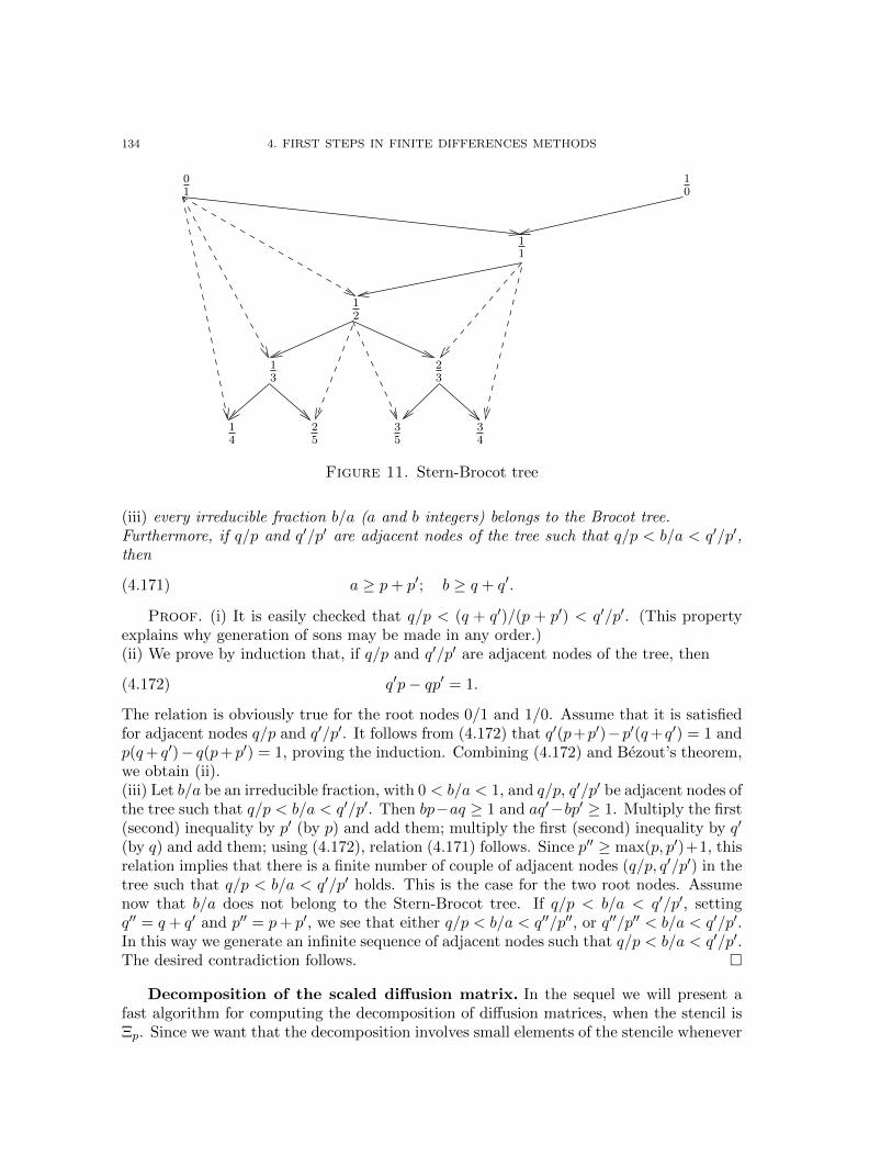
134 4. FIRST STEPS IN FINITE DIFFERENCES METHODS
14
25
35
34
13
23
12
11
01
10
Figure 11. Stern-Brocot tree
(iii) every irreducible fraction b/a (a and b integers) belongs to the Brocot tree.Furthermore, if q/p and q′/p′ are adjacent nodes of the tree such that q/p < b/a < q′/p′,then
(4.171) a ≥ p+ p′; b ≥ q + q′.
Proof. (i) It is easily checked that q/p < (q + q′)/(p + p′) < q′/p′. (This propertyexplains why generation of sons may be made in any order.)(ii) We prove by induction that, if q/p and q′/p′ are adjacent nodes of the tree, then
(4.172) q′p− qp′ = 1.
The relation is obviously true for the root nodes 0/1 and 1/0. Assume that it is satisfiedfor adjacent nodes q/p and q′/p′. It follows from (4.172) that q′(p+p′)−p′(q+q′) = 1 andp(q+ q′)− q(p+ p′) = 1, proving the induction. Combining (4.172) and Bezout’s theorem,we obtain (ii).(iii) Let b/a be an irreducible fraction, with 0 < b/a < 1, and q/p, q′/p′ be adjacent nodes ofthe tree such that q/p < b/a < q′/p′. Then bp−aq ≥ 1 and aq′−bp′ ≥ 1. Multiply the first(second) inequality by p′ (by p) and add them; multiply the first (second) inequality by q′
(by q) and add them; using (4.172), relation (4.171) follows. Since p′′ ≥ max(p, p′)+1, thisrelation implies that there is a finite number of couple of adjacent nodes (q/p, q′/p′) in thetree such that q/p < b/a < q′/p′ holds. This is the case for the two root nodes. Assumenow that b/a does not belong to the Stern-Brocot tree. If q/p < b/a < q′/p′, settingq′′ = q + q′ and p′′ = p+ p′, we see that either q/p < b/a < q′′/p′′, or q′′/p′′ < b/a < q′/p′.In this way we generate an infinite sequence of adjacent nodes such that q/p < b/a < q′/p′.The desired contradiction follows.
Decomposition of the scaled diffusion matrix. In the sequel we will present afast algorithm for computing the decomposition of diffusion matrices, when the stencil isΞp. Since we want that the decomposition involves small elements of the stencile whenever

4. GENERALIZED FINITE DIFFERENCES 135
Ω
1
1
0
1
1
2
1
3
2
3
1
4
3
4
Figure 12. Correspondence of directions
possible we will use only in the decomposition the set of directions with integer irreduciblecomponents.
As discussed before, it suffices to discuss the case when the matrix ah is in outer regionI; i.e., when it is positive semidefinite and non diagonally dominant, and a22 < a12 < a11.On figure 12, this means that the view of ah belongs to the quarter of ball in the upperright side, and is not in the triangle with vertices of coordinates (0, 0), (1, 0) and (0, 1).The latter correspond to the identity matrix, and to degenerate diffusions with horizontaland angle of π/4 diffusions. (The cone generated by these three points is a set of diagonallydominant matrices).
With every node q/p of the Stern-Brocot tree, q ≤ p, associate directions ξp,q :=
(p q)> and Xp,q := ξp,qξ>p,q. With two adjacent nodes is associated the plane H(q/p, q′/p′)
generated by Xp,q and Xp′,q′ , and two half spaces, the inner one (containing the identitymatrix) and the outer one. If p/q > p′/q′, let y := View(Xp,q) ∧ View(Xp′,q′) (wherehere ∧ denote the vector product in R2). Then a matrix a belongs to the outer region iffy · View(a) ≥ 0, see figure 12. Denote by PH(q/p, q′/p′) the orthogonal projection ontothis plane (projection w.r.t. the Frobenius norm is equivalent to the Euclidean projectionin the image space R3).
Beginning the search of a decomposition, we are in the following situation : the matrixah belongs to the outer half space of H(0/1, 1/1). So, let us assume more generally that ah
belongs to the outer half space of H(q/p, q′/p′), where q/p and q′/p′ are adjacent nodes. Infigure 12 we have drawn the views of the first nodes of the Stern-Brocot tree; the segmentsare the views of the segment between two neighbouring nodes of this tree.
We see, using lemma 4.60 that we have to use another element of stencil of the formq/p, with q and p nonnegative, such that q/p < q/p < q′/p′, and as small as possible. Inview of (4.171), the optimal choice is to take the child q′′/p′′ = (q + q′)/(p + p′). Then(see figure 12) there are two possibilities :
- The matrix ah belongs to both inner half spaces of H(q/p, q′′/p′′) and H(q′′/p′′, q′/p′).Then ah belongs to the cone generated by Xp,q, Xp′,q′ and Xp′′,q′′ . Since these threematrices are linearly independant, the corresponding coefficients are unique nonnegative

136 4. FIRST STEPS IN FINITE DIFFERENCES METHODS
solution of the invertible (three dimensional) system
(4.173) ηp,q Xp,q + ηp′,q′ Xp′,q′ + ηp′′,q′′ Xp′′,q′′ = ah.
- The matrix ah belongs to at least one outer half space. Since Xp′′,q′′ belongs to the
boundary of the cone of positive semidefinite matrices, ah cannot belong to both outerhalf spaces (see figure 12). We are therefore lead to the situation at the beginning, settingeither q/p or q′/p′ to q′′/p′′.
If p′′ > pmax, we replace ah by its projection onto the cone generated by matrices ofthe form Xpi,qi , with either qi/pi < q/p or q′/p′ < qi/pi. Note that this projection belongsto the cone generated by Xp,q and Xp′,q′ . As above, since these two matrices are linearlyindependant, the corresponding coefficients are unique nonnegative solution of the system
(4.174) ηp,q Xp,q + ηp′,q′ Xp′,q′ = PH(q/p, q′/p′) ah.
This leads to an effective algorithm, that will stop either if the exact decompositionis obtained, or if either p′′ > pmax, or if the projection of ah onto H(q/p, q′/p′) is closeenough to ah. The precise algorithm is as follows; ε is a threshold for the distance to theprojection of ah onto the class of consistent matrices, and pmax is the size of stencil:
Algorithm DECOMPinitial phase: Data ε ≥ 0, pmax > 0. Set k := 0.• If ah is diagonally dominant: set η using (4.170) and stop.• Reduction to region I, i.e. ah22 < ah12 < ah11.
Set q0/p0 := 0/1, q′0/p′0 := 1/1.
repeat• Compute a′ := PH(q/p, q′/p′)ah.• If ‖a′− ah‖ ≤ ε‖ah‖ or p+ p′ > pmax: compute η, decomposition of a′ using
(4.174) and stop.• Set q′′/p′′ := (q + q′)/(p+ p′).• If ah in inner half spaces of H(q/p, q′′/p′′) and H(q/p, q′′/p′′): compute η
using (4.173) and stop.• If a is in outer half space of H(q/p, q′′/p′′): q′/p′ := q′′/p′′.
Otherwise q/p := q′′/p′′.• k := k + 1 .
end repeat
From the above discussion we have the following result.
Theorem 4.63. Algorithm DECOMP provides a decomposition of ah with a relativeerror lower than ε, and stops after at most pmax iterations. The cost of each iteration isO(1) operations, and hence, its total cost is no more than O(pmax).
We plot in figure 14 the values of the numerical errors when the space steps vanish,for various values of p; see details of the model in [11]. As expected, the higher p, thebetter the precision.
5. Error estimates
5.1. Basic analysis based on consistency and simple monotonicity. We ana-lyze the error estimates in the case of the one dimensional space equation (4.1), assuming

5. ERROR ESTIMATES 137
η
η 0
θ
O 1 2 3
a
2 θ
Ω
a0
Figure 13. Correspondence of angles
−1.6 −1.4 −1.2 −1 −0.8 −0.6 −0.4 −0.2−2.6
−2.4
−2.2
−2
−1.8
−1.6
−1.4
−1.2
log10 ∆ x
log10 e
p = 4
p = 2
p = 1
p =10
Figure 14. Numerical error, for various values of p.
that (4.1) has a smooth solution V (i.e., with bounded derivatives of sufficiently largeorder). Denote by vkj the solution of the explicit scheme
(4.175)
vkj − vk−1j
h0+ (bkj )+
vkj+1 − vkjh1
+ (bkj )−vkj − vkj−1
h1
+12a
kj
vkj+1 + vkj−1 − 2vkjh2
1
− rkj vkj + fkj = 0, j ∈ Z, k = 1 : N,
vNj = g(xj), j ∈ Z,
We easily check that the scheme is simply monotonic whenever the following conditionholds:
(4.176) h0
(‖r‖∞ +
‖b‖∞h1
+‖a‖∞h2
1
)≤ 1.

138 4. FIRST STEPS IN FINITE DIFFERENCES METHODS
Set vkj := V (xj , tk). We may view v as a solution of the discretized scheme with a perturbedr.h.s.:
(4.177)
vkj − vk−1j
h0+ (bkj )+
vkj+1 − vkjh1
+ (bkj )−vkj − vkj−1
h1
+12a
kj
vkj+1 + vkj−1 − 2vkjh2
1
− rkj vkj + fkj = ekj , j ∈ Z, k = 1 : N,
vNj = gj , j ∈ Z,
where the consistency error ekj of the scheme can be decomposed as a sum of contributionsof the terms of time derivative, transport and diffusion:
(4.178) ekj = ek0,j + ek1,j + ek2,j ,
with
(4.179) ek0,j :=vkj − v
k−1j
h0− Vt(xj , tk),
(4.180) ek1,j := (bkj )+
vkj+1 − vkjh1
+ (bkj )−vkj − vkj−1
h1− bkjVx(xj , tk),
(4.181) ek2,j := 12a
kj
(vkj+1 + vkj−1 − 2vkj
h21
− Vxx(xj , tk)
).
Lemma 4.64. Assume that inf r ≥ 0 and that the monotonicity condition (4.176) holds.Then the following error estimate holds:
(4.182) supk,j|V (xj , tk)− vkj | ≤ T sup
k,j|ekj |.
Proof. Since vkj := V (xj , tk) − vkj is solution of the same scheme with zero final
condition and source term −ekj , this is an immediate consequence of lemma 4.9.
Assume now that the function V is smooth with bounded derivatives of any order.Using standard first-order Taylor expansions with integral remainders of vt and vx, weobtain
(4.183)∣∣∣ek0,j∣∣∣ =
∣∣∣∣∫ 1
0(Vt(xj , tk − h0s)− Vt(xj , tk)) ds
∣∣∣∣ ≤ ‖Vtt‖∞h0,
and similarly
(4.184)
∣∣∣∣∣ vkj±1 − vkjh1
− Vx(xj , tk)
∣∣∣∣∣ ≤ ‖Vxx‖∞h1 ⇒∣∣∣ek1,j∣∣∣ ≤ ‖b‖∞‖Vxx‖∞h1.
Next consider the following third order expansion (we skip the time argument and take ±equal to either 1 or -1 everywhere)
(4.185) V (x± h1) = V (x)± Vx(x)h1 + 12h
21Vxx(x)± 1
2h31
∫ 1
0(1− s)2Vxxx(x± sh1)ds.

5. ERROR ESTIMATES 139
Summing the above two equalities for ±1 and x = xj , we obtain(4.186)∣∣∣∣∣ vkj+1 + vkj−1 − 2vkj
h21
− Vxx(xj , tk)
∣∣∣∣∣ ≤ h1
2
∫ 1
0(1− s)2 |Vxxx(x+ sh1)− Vxxx(x− sh1)|ds.
Using |Vxxx(x+ sh1)− Vxxx(x− sh1)| ≤ 2‖Vxxxx‖∞h1, we obtain that an upper bound ofthe r.h.s. is ‖Vxxxx‖∞h2
1, and therefore
(4.187)∣∣∣ek2,j∣∣∣ ≤ 1
2‖a‖∞‖Vxxxx‖∞h21.
Note that since this is an even order derivative and successive grid points are equidistant,we have one error order more than for the other error terms. Combining the previousestimates we get
(4.188) ‖e‖∞ ≤ ‖Vtt‖∞h0 + ‖b‖∞‖Vxx‖∞h1 + 12‖a‖∞‖Vxxxx‖∞h
21.
We deduce then from lemma 4.64 the following error estimate.
Theorem 4.65. For the scheme (4.70), we have the following error estimate:
(4.189) supj,k
∣∣∣V (xj , tk)− vkj∣∣∣ ≤ T (‖Vtt‖∞h0 + ‖b‖∞‖Vxx‖∞h1 + 1
2‖a‖∞‖Vxxxx‖∞h21
).
Exercice 4.66. Derive similar estimates for the implicit or semi implicit schemes, andfor problems with space dimension greater than one.
As we will see, the solution of (4.1) is not always not so smooth, and this will lead usto introduce a method of regularization by convolution in order to obtain error estimatesin the general case.
5.2. Smoothness of the solution of (4.1). We recall the notion of Holderian map-pings.
Definition 4.67. Let E ⊂ Rn. We say that w : E → R is Holder with constantCw ≥ 0 and exponent µw ∈ (0, 1] (or with constants (Cw, µw)), if the following holds:
(4.190) |w(x)− w(y)| ≤ Cw|x− y|µw , for all x, y in E.
Note that, if µw = 1 we recover the definition of a Lipschitz function. More generally,for w : R × [0, T ] → R, we denote by µw,x, µw,t in (0, 1] the Holder exponents w.r.t. xand t; these are (whenever they exist) the biggest constants in (0, 1] such that, for someCw > 0:
(4.191)∣∣w(x′, t′)− w(x, t)
∣∣ ≤ Cw (|x′ − x|µw,x + |t′ − t|µw,t), for all x and t.
Consider the space of bounded functions that are Lipschitz in space and Holder withexponent 1/2 in time:
(4.192) V1,1/2 := w : R× [0, T ]→ R bounded; µw,x = 1, µw,t = 1/2 .
Remark 4.68. Usually, in financial applications, using the Feynman Kac-formula,which gives a representation as an expectation of a cost associated to some stochasticprocess, one can usually associate with a pair (f, g), with
(4.193) f ∈ V1,1/2 and g is Lipschitz and bounded,

140 4. FIRST STEPS IN FINITE DIFFERENCES METHODS
a solution V [f, g] of the PDE in the sense of viscosity solutions (s ee e.g. Fleming andSoner [29]), and this solution is (see e.g. Krylov [38]) which is the unique solution in V1,1/2
and such that, if V 1 = V [f1, g1] and V 2 = V [f2, g2], then for some c > 0 not dependingon (f1, f2, g1, g2):
(4.194) ‖V 2 − V 1‖∞ ≤ c(‖f2 − f1‖∞ + ‖g2 − g1‖∞
).
Remark 4.69. It may happen that the solution is more regular. In some cases includ-ing the one of the heat equation, if f ∈ V1,1/2 and g is bounded and has Lipschitz secondderivatives, the solution V is such that Vt, Vx, Vxx are functions in V1,1/2; see Krylov [37,Thm. 9.1.2]. For financial applications, such hypotheses are however too strong.
Exercice 4.70. Consider the heat equation with final condition g(x) = x+. ComputeV (0, t) using e.g. (1.32). Deduce that we cannot have in general more than the 1/2 Holderexponent in time.
Remark 4.71. We will obtain in chapter 2 additional regularity results, needing inparticular the diffusion matrix to be uniformy elliptic.
We see that we cannot in general apply theorem 4.65 since the solution V of the PDEis not smooth enough. However we can regularize V by convolution and see if it is solutionof a PDE close to the original one. This is the subject of the next section.
5.3. Regularization by convolution. We next present an approach that allowsto obtain error estimates when the solution of the PDE is Holder, but not necessarilydifferentiable, as is typically the case in applications.
We recall the definition of regularizing kernels and ε regularization in definition 2.7.of chapter 2. So, let ψε(x) := ε−nψ(x/ε) a regularizing kernel. Let w be a bounded,Holder function over Rn, with Holder constants Cw > 0, µw ∈ (0, 1]. We recall that its εregularization (by the regularizing kernel ψε) is defined as wε(x) := ψε ∗ w, i.e.
(4.195) wε(x) =
∫Rnw(y)ψε(x− y)dy =
∫Rnw(x− y)ψε(y)dy =
∫Rnw(x− εz)ψ(z)dz,
where we have made the change of variables z = y/ε. Since
(4.196) wε(x)− w(x) =
∫Rn
(w(x− εz)− w(x))ψ(z)dz,
it follows that
(4.197) ‖wε‖∞ ≤ ‖w‖∞ and ‖wε − w‖∞ ≤ εµwCw.
Call multiindex an element of Nn. With each multiindex α is associated the differentialoperator
(4.198) Dα :=∂α1
∂xα11
· · · ∂αn
∂xαnn, of order |α| :=
n∑i=1
αi.
In view of (4.195), wε is of class C∞ and satisfies
(4.199) Dαwε(x) =
∫Rnw(x− y)Dαψε(y)dy, for any multiindex α.

5. ERROR ESTIMATES 141
Since Dαψε(y) = ε−|α|−nDαψ(y/ε), with the change of variable z = y/ε, we get
(4.200) Dαwε(x) = ε−|α|∫Rnw(x−y)Dαψ
(yε
)d(yε
)= ε−|α|
∫B(0,1)
w(x−εz)Dαψ(z)dz.
In addition, if α 6= 0,∫B(0,1)D
αψ(z)dz = 0, and therefore we also have
(4.201) Dαwε(x) = ε−|α|∫B(0,1)
(w(x− εz)− w(x))Dαψ(z)dz, if α 6= 0.
We deduce that
(4.202) ‖Dαwε‖∞ ≤ εµw−|α|Cw‖Dαψ‖1, if α 6= 0.
Remark 4.72. We can refine this estimate for α = β + γ, with β and γ multiindexes,when Dβw exists and is itself bounded and Holder. Indeed, since Dβwε = ψε ∗Dβw andDαwε(x) = Dγ
(Dβwε
), applying (4.200) with (Dβw, γ) in lieu of (w,α), we obtain:
(4.203) Dαwε(x) =
∫RnDβw(y)Dγψε(x− y)dy = ε−|γ|
∫RnDβw(x− εz)Dγψ(z)dz.
Let us denote by (Cw,β, µw,β) the Holder constants of Dβw. Applying now (4.202) with
again Dβw(y) and γ in lieu of w(y) and α, we get:
(4.204) ‖Dαwε‖∞ ≤ εµw,β−|γ|Cw,β‖Dγψ‖1, if γ 6= 0.
Anisotropic spaces. We have seen that we need to consider functions of space andtime that are Lipschitz in space and Holder in time with exponent 1
2 . So consider ψ :
Rn+1 → R+ of class C∞ (elements of Rn+1 denoted by (x, t) with x ∈ Rn) such that
(4.205)
∫ψ(x)dx = 1; suppψ ⊂ B,
where
(4.206) B := (x, t) ∈ Rn+1; |x|+√|t| ≤ 1.
Note that B ⊂ B (the Euclidean unit ball). Redefine ψε and wε as
(4.207) ψε(x, t) = ε−n−2ψ(x/ε, t/ε2); wε := ψε ∗ w.Note that ψε is nonnegative with integral 1, and satisfies
(4.208) suppψε ⊂ (x, t) ∈ Rn+1; |x|+√|t| ≤ ε ⊂ εB.
A multiindex in this setting is of the form α = (αx, αt) ∈ Nn×N, with associated differentialoperator
(4.209) Dα :=∂|αx|
∂xα11 · · · ∂x
αnn
(∂αt
∂tαt
).
We assume that w is Lipschitz in space and Holder with exponent 1/2 in time:(4.210)
|w(x′, t′)− w(x, t)| ≤ Cw(|x′ − x|+ |t′ − t|1/2
), for all (x′, t′) and (x, t) in Rn+1.
Let us set
(4.211) wε(x, t) :=
∫Rn+1
w(x− y, t− s)ψε(y, s)d(y, s).

142 4. FIRST STEPS IN FINITE DIFFERENCES METHODS
Setting z := y/ε and τ := s/ε2, we obtain
(4.212) wε(x, t) =
∫B(0,1)
w(x− εz, t− ε2τ)ψ(z, τ)d(z, τ).
It follows that
(4.213) ‖wε‖∞ ≤ ‖w‖∞; ‖wε − w‖∞ ≤ Cwε.
Similarly, for a multiindex α 6= 0 we have that
(4.214)
Dαwε(x, t) = ε−|αx|−2|αt|∫Rn+1
w(x− y, t− s)Dαψ(yε,s
ε2
)d(yε,s
ε2
)= ε−|αx|−2|αt|
∫B(0,1)
w(x− εz, t− ε2τ)Dαψ(z, τ)d(z, τ),
and again we may write if α 6= 0:
(4.215) Dαwε(x, t) = ε−|αx|−2|αt|∫B(0,1)
(w(x− εz, t− ε2τ)− w(x, t))Dαψ(z, τ)d(z, τ).
Therefore, denoting by Cw the Holder coefficient of w, we have that, using an adaptationto the present setting of (4.201):
(4.216) ‖Dαwε‖∞ ≤ ε1−|αx|−2|αt|Cw‖Dαψ‖1, when α 6= 0.
5.4. Error estimates in the case of constant coefficients. We next apply the ap-proach of regularization by convolution in the simple case of the PDE (4.1), with constantcoefficients a, b, r.
Theorem 4.73. Let (4.193)-(4.194) hold, and (a, b, r) be constant. Let v be the solutionof the explicit scheme (4.175), such that the monotonicity condition (4.176) holds. Then,for some c > 0 not depending on h and ε ∈ (0, 1]:
(4.217) supj,k
∣∣∣V (xj , tk)− vkj∣∣∣ ≤ c (ε+ ε−3h0 + ε−1h1 + ε−3h2
1
).
In particular, when h0 = O(h21) (monotonicity condition), taking ε = O(h
1/21 ) we deduce
that
(4.218) supj,k
∣∣∣V (xj , tk)− vkj∣∣∣ = O
(h
1/21
).
Proof. It suffices to prove the first statement. We first extend f and V for t ∈ [−1, 0)by setting f(x, t) := f(x, 0), t ∈ [−1, 0) < 0, and by taking V as the solution of the PDEextended for t ∈ [−1, 0).
Remember that ψε was defined in (4.207). We may assume that ψ(x, t) = 0 if t ≤ 0.Then f ε := f ∗ ψε and V ε := V ∗ ψε are well-defined, for (x, t) ∈ R × [0, T ] and ε ≤ 1.Computing the convolution of both sides of (4.1) with ψε, we find that V ε is solution ofthe perturbed PDE
(4.219)
V εt + bV ε
x + 12aV
εxx − rV ε + f ε = 0, (x, t) ∈ R× [0, T ],
V ε(x, T ) = gε(x), x ∈ R,
5. ERROR ESTIMATES 143
where gε(x) := V ε(x, T ) for all x ∈ Rn. Since V in V1,1/2, we easily get that
(4.220) ‖f ε − f‖∞ + ‖gε − g‖∞ = O(ε).
By (4.194), we have that
(4.221) ‖V − V ε‖∞ = O(ε).
Next, denote by vε the solution of the scheme (4.175), with (f ε, gε) in lieu of (f, g). Bythe `∞ estimates for this Markovian scheme, combined with (4.220), we know that
(4.222) supj,k|vkj − v
ε,kj | ≤ ‖g
ε − g‖∞ + T‖f ε − f‖∞ = O(ε).
In view of the above inequalities and of the triangle inequality
(4.223) supj,k|V (xj , tk)− vkj | ≤ ‖V − V ε‖∞ + sup
j,k|V ε(xj , tk)− vε,kj |+ sup
j,k|vε,kj − v
kj |,
it suffices to check that the second term in the above r.h.s. is of order of the r.h.s. of(4.217). We apply theorem 4.65 to the scheme with perturbed data. The norms of partialderivatives of V ε are estimated thanks to (4.216):
(4.224) ‖D2t2V
ε‖∞ = O(ε−3); ‖D2x2V
ε‖∞ = O(ε−1); ‖D4x4V
ε‖∞ = O(ε−3).
The conclusion follows.
5.5. Error estimates in the case of a constant diffusion matrix. We will nowextend the theory of error estimates based on the regularization by convolution in the caseof variable coefficients. We will use, however, the important restriction that the diffusioncoefficient is assumed to be constant.
Theorem 4.74. Let (4.193)-(4.194) hold, b, r belong to V1,1/2, and the diffusion matrixa be constant. Let v be the solution of the explicit scheme (4.70). Then again (4.217)-(4.218) hold.
Proof. The proof is similar to the one of theorem 4.73, with some minor adaptations.Again only(4.217) needs to be proved. We first extend b, r, f for t ∈ [−1, 0) by setting
(4.225) φ(x, t) := φ(x, 0), t < 0, for φ = b, r, f ,
and by taking V as the solution of the PDE extended for t ∈ [−1, 0). We may assumethat ψ(x, t) = 0 if t ≤ 0. Then f ε := f ∗ ψε and V ε := f ∗ ψε are well-defined, for(x, t) ∈ R× [0, T ]. Applying the convolution with ψε on both sides of the first relation in(4.1), we obtain that V ε is solution of
(4.226)
V εt + b(x, t)V ε
x + 12aV
εxx − r(x, t)V ε + f ε(x, t) = 0, (x, t) ∈ R× [0, T ],
V ε(x, T ) = gε(x), x ∈ R.
where gε(x) := V ε(x, T ), the source terme f ε(x, t) taking into account the variations of band r:
(4.227) f ε(x, t) := f ε(x, t) + eε1(x, t)− eε2(x, t),

144 4. FIRST STEPS IN FINITE DIFFERENCES METHODS
with eε1 = (bVx) ∗ ψε − b(Vx ∗ ψε) and eε2 = (rV ) ∗ ψε − r(V ∗ ψε), i.e.,
(4.228)
eε1(x, t) :=
∫ψε(y, s)(b(x− y, t− s)− b(x, t))Vx(x− y, t− s)dyds,
eε2(x, t) :=
∫ψε(y, s)(r(x− y, t− s)− r(x, t))V (x− y, t− s)dyds.
Since V and Vx are bounded, It follows that ‖eε1‖∞ + ‖eε2‖∞ = O(ε), and hence, ‖f ε −f‖∞ + ‖gε − g‖∞ = O(ε). We conclude the proof as we did for the one of theorem 4.73,after (4.220).
Exercice 4.75. Derive similar estimates for the implicit or semi implicit schemes, andfor problems with space dimension greater than one.
Remark 4.76. The above method has a straightforward extension to the case whenthe diffusion coefficient is variable, whenever the solution of a PDE has a Lipschitz spatialgradient (i.e., when Vxx is essentially bounded). However, this assumption is not alwayssatisfied in applications. For variable diffusion coefficients one uses the “coefficients shak-ing” method introduced by Krylov, in the context of HJB equations; see e.g. Barles andJakobsen [6], Bonnans et al. [13], Krylov [38].
5.6. Centered scheme. We now study the centered scheme (4.74), assuming that(4.77) holds, so that this scheme is simply monotonic by lemma 4.23. We briefly indicatewhere are the changes in the analysis. Form the Taylor expansions (skipping the timeargument)
(4.229) V (x± h1) = V (x)± h1Vx(x) + h21
∫ 1
0(1− s)Vxx(x± sh1)ds
we deduce that∣∣∣∣V (x+ h1)− V (x− h1)
2h1− Vx(x)
∣∣∣∣ ≤ h1
∫ 1
0(1− s)|Vxx(x+ sh1)− Vxx(x− sh1)|ds
≤ h21‖Vxxx‖∞.
Following otherwise the analysis of the upwind scheme (theorem 4.65) we deduce that:
Theorem 4.77. For the centered scheme (4.74), assuming (4.77) holds and the solu-tion V of the PDE to be smooth enough, we have the following error estimate:
(4.230) supj,k
∣∣∣V (xj , tk)− vkj∣∣∣ ≤ T (‖Vtt‖∞h0 + ‖b‖∞‖Vxxx‖∞h2
1 + 12‖a‖∞‖Vxxxx‖∞h
21
).
If V is Holder, following the analysis of theorem 4.73 we deduce that:
Theorem 4.78. Let (4.193)-(4.194) hold, and (a, b, r) be constant. Let v be the solutionof the centered scheme (4.74), assuming that (4.77) holds Then, for some c > 0 notdepending on h and ε ∈ (0, 1]:
(4.231) supj,k
∣∣∣V (xj , tk)− vkj∣∣∣ ≤ c (ε+ ε−3h0 + ε−2h2
1 + ε−3h21
).
In particular, when h0 = O(h21) (monotonicity condition), taking ε = O(h
1/21 ) we deduce
that
(4.232) supj,k
∣∣∣V (xj , tk)− vkj∣∣∣ = O
(h
1/21
).
6. DISCRETE PARABOLIC ENERGY ESTIMATES 145
Exercice 4.79. Extend this analysis to the implicit centered scheme (4.83).
6. Discrete parabolic energy estimates
6.1. Overview. It is useful to check the stability of the solution of the numericalschemes in (weighted) L2 norms. This is a desirable property, especially in the case of θschemes, or of some schemes for dimension greater than 1, for which simple monotonicitydoes not always hold. Doing this we will obtain the discrete counterparts of the first ansecond parabolic energy estimates. So, consider the following PDE
(4.233) Vt(x, t) + b(x, t)Vx(x, t) + 12a(x, t)Vxx(x, t) = 0,
with x ∈ R, t ∈ [0, T ], a(x, t) > 0, and the final condition
(4.234) V (x, T ) = g(x), x ∈ R.
We will recall the classical energy inequalities in the case of constant coefficients, andextend them to the case when a and b are Lipschitz functions of the space variables. Wewill conclude the section with the analysis of θ schemes, and show that they satisfy energyestimates when θ ≥ 1/2.
As usual we denote by h0 > 0 and h1 > 0 the time and space steps, with h0 = T/N ,N ∈ N. We set xj = jh1, j ∈ Z, and tk = kh0, k = 0 to N . The algorithm approximates
V (xj , tk) by ukj .
Over the space `2Z (set of sequences (vj)j∈Z with summable squares) we define the(scaled) norm and associated scalar product by
(4.235) ‖v‖2h := h1
∑j
(vj)2; (u, v)h := h1
∑j
ujvj .
We denote by `2h the space `2Z endowed with the above norm, and assume that there existsCg > 0 such that
(4.236) h1
∑j
|g(xj)|2 ≤ C2g <∞, for all h1 > 0.
The operators δ1, Dh and ∆h (discrete unit translation, gradient and Laplacian) are definedby
(4.237) (δ1v)j = vj+1; (Dhv)j :=vj+1 − vj
h1; (∆hv)j :=
vj+1 + vj−1 − 2vjh2
1
.
We adopt the usual abuse of notation Dhvj := (Dhv)j and ∆hvj := (∆hv)j . For u, v in`2h we easily check the discrete integration by parts formula
(4.238) − h1
∑j
(∆hu)jvj = (Dhu,Dhv)h, for all u, v in `2h.
6.2. Constant coefficients. In this section we assume that a ≥ 0 and b are constant;we may assume that b ≥ 0. Consider the standard implicit finite differences (upwind)scheme
(4.239)uk+1j − ukjh0
+ bDhukj + 1
2a∆hukj + fkj = 0; j ∈ Z, k = 0, . . . , N − 1,

146 4. FIRST STEPS IN FINITE DIFFERENCES METHODS
with final condition
(4.240) uNj = g(xj), j ∈ Z.This scheme is known to be simply monotonic.
6.2.1. First discrete parabolic energy estimates. We start by the simple case when thesource term is equal to 0.
Lemma 4.80. Assume that f = 0. Then the solution of (4.239) satisfies
(4.241) ‖uk‖2h + h0a‖Dhuk‖2h ≤ ‖uk+1‖2h
and
(4.242) max
(maxk‖uk‖2h, h0a
N−1∑k=0
‖Dhuk‖2h
)≤ ‖uN‖2h.
Proof. Multiplying (4.239) by h0, we obtain
(4.243) ukj − 12h0a∆hu
kj = uk+1
j + h0bDhukj , j ∈ Z, k = 0, . . . , N − 1.
Multiplying by h1ukj and summing over j, we get with (4.238)
(4.244) ‖uk‖2h + 12h0a‖Dhu
k‖2h ≤ (uk+1, uk)h + bh0
h1(δ1u
k − uk, uk)h.
Now ‖δ1uk‖h = ‖uk‖h, and so by the Cauchy-Schwarz inequality
(4.245) (δ1uk − uk, uk)h ≤ ‖δ1u
k‖h‖uk‖h − ‖uk‖2h = 0.
By the Young inequality,
(4.246) (uk+1, uk)h ≤ 12(‖uk‖2h + ‖uk+1‖2h).
Combining relations (4.244)-(4.246), we get (4.241). Summing from k to N −1, we obtain
(4.247) ‖uk‖2h + h0aN−1∑`=k
‖Dhu`‖2h ≤ ‖uN‖2h, for all k = 0 to N − 1,
from which (4.242) easily follows.
In the sequel we need the following technical lemma;
Lemma 4.81. Let c > 0. For all ε > 0, For h0 > 0 is small enough, then
(4.248) (1− ch0)−N ≤ e(c+ε)T .
Proof. For h0 > 0 is small enough, we have that log(1− ch0) ≥ −(c+ ε)h0, and so,
(4.249) (1− ch0)−N = e−N log(1−ch0) ≤ eN(c+ε)h0) = e(c+ε)T ,
as was to be proved.
Lemma 4.82. Let fk ∈ `2h for all k and ε > 0. If h0 is small enough, the solution of(4.239) satisfies
(4.250) maxk‖uk‖2h + h0a
N−1∑k=0
‖Dhuk‖2h ≤ eT+ε
(‖uN‖2h + h0
n−1∑k=0
‖fk‖2h
).

6. DISCRETE PARABOLIC ENERGY ESTIMATES 147
Proof. Repeating the arguments of the proof of lemma 4.82 we obtain that
(4.251)‖uk‖2h + h0a‖Dhu
k‖2h ≤ ‖uk+1‖2h + 2h0(fk, uk)h≤ ‖uk+1‖2h + h0(‖fk‖2h + ‖uk‖2h)
so that in particular
(4.252) (1− h0)‖uk‖2h ≤ ‖uk+1‖2h + h0‖fk‖2h,
and so with lemma 4.81, when h0 > 0 is small enough:
(4.253)‖uk‖2h ≤ (1− h0)k−N
(‖uN‖2h + h0
∑N−1`=k ‖f `‖2h
),
≤ eT+ε(‖uN‖2h + h0
∑N−1`=0 ‖f `‖2h
),
as was to be proved.
6.2.2. A refined first discrete parabolic energy estimates. Consider the function space
(4.254) Vh := u ∈ `2h; Dhu ∈ `2h,
which is an Hilbert space when endowed with the norm
(4.255) ‖u‖Vh :=(‖u‖2h + ‖Dhu‖2h
)1/2.
We can obtain an estimate of the type (4.250) with the norm of fk in the dual of Vh(rather than `2h). We leave the proof as an exercice.
6.2.3. Second discrete parabolic energy estimates.
Lemma 4.83. Let fk ∈ `2h for all k, and uN ∈ Vh. Then the solution of (4.239) satisfiesfor some c > 0, not depending on (f, g):
(4.256) maxk‖Dhu
k‖h + h−10
N−1∑k=0
‖uk+1 − uk‖2h ≤ c
(‖uN‖2V + h0
n−1∑k=0
‖fk‖2h
).
Proof. Multiplying (4.239) by (uk+1j − ukj ), summing over j and using (4.238), we
obtain that(4.257)1
h0‖uk+1
j −ukj ‖2h+12a‖Dhu
k‖2h = 12a(Dhu
k, Dhuk+1)h+(fk, ukj−uk+1
j )h+b(Dhuk, uk−uk+1)h.
Use
(Dhuk, Dhu
k+1)h ≤ 12(‖Dhu
k‖2h + ‖Dhuk+1‖2h),(4.258)
(fk, ukj − uk+1j )h ≤ 1
2h0‖fk‖2h +1
2h0‖uk+1
j − ukj ‖2h,(4.259)
b(Dhuk, uk − uk+1)h ≤ h0b
2‖Dhuk‖2h +
1
4h0‖uk+1
j − ukj ‖2h.(4.260)
It follows that
(4.261)1
4h0‖uk+1
j − ukj ‖2h + (a
4− h0b
2)‖Dhuk‖2h ≤
a
4‖Dhu
k+1‖2h + 12h0‖fk‖2h.

148 4. FIRST STEPS IN FINITE DIFFERENCES METHODS
Summing inequalities (4.261) from k to N − 1, we get
1
4h0
N−1∑`=k
‖uk+1j − ukj ‖2h +
a
4‖Dhu
k‖2h ≤a
4‖Dhu
N‖2h + h0b2N−1∑`=k
‖Dhu`‖2h + 1
2h0
N−1∑`=k
‖f `‖2h.
The conclusion follows since we can estimate the r.h.s. thanks to lemma 4.250.
6.3. Varying coefficients. We now assume that inf a = α > 0 and that a = a(x, t)and b = b(x, t) are uniformly Lipschitz w.r.t. the space variable: for all t ∈ [0, T ] and x,x′ in R, we have that
(4.262)
inf a = α > 0, and for all x, x′ in R :|a(x′, t)− a(x, t)| ≤ La|x′ − x|,|b(x′, t)− b(x, t)| ≤ Lb|x′ − x|.
For the sake of simplicity we also assume that f = 0. Setting akj = a(xj , tk) and bkj =
b(xj , tk), the expression of the upwind implicit discretization scheme is now
(4.263)uk+1j − ukjh0
+(bkj )+Dhukj+(bkj )−Dhu
kj−1+ 1
2akj∆hu
kj = 0; j ∈ Z, k = 0, . . . , N−1,
with the same final condition (4.240).
Lemma 4.84. Set cab := 12(La)
2/α+ 2Lb. Let ε > 0. If (h0, h1) is small enough, thenthe solution of the scheme (4.263) satisfies
(4.264)
(i) max
k‖uk‖2h ≤ e(cab+ε)T ‖uN‖2h,
(ii) 12h0α
N−1∑k=0
‖Dhuk‖2h ≤
(1 + Tcabe
(cab+ε)T)‖uN‖2h.
Proof. Multiplying (4.263) by 2h0h1ukj and summing over j, we obtain with (4.246):
(4.265)
‖uk‖2h − h0h1
∑j
akjukj∆hu
kj ≤ ‖uk+1‖2h + 2h0h1
∑j
((bkj )+Dhu
kj + (bkj )−Dhu
kj−1
)ukj .
Use
(4.266)
−h1∑
j akj∆hu
kju
kj = −
∑j
(Dhukj −Dhu
kj−1)akju
kj ,
=∑j
Dhukj (a
kj+1u
kj+1 − akjukj ),
= h1
∑j
akj |Dhukj |2 + h1
∑j
akj+1 − akjh1
Dhukju
kj+1,
≥ α‖Dhuk‖2h − La‖Dhu
k‖h‖uk‖h.
Also, since 2(γ − δ)δ ≤ γ2 − δ2 for all γ, δ:
(4.267)
2∑j
(bkj )+(ukj+1 − ukj )ukj ≤∑j
(bkj )+
((ukj+1)2 − (ukj )
2),
=∑j
((bkj−1)+ − (bkj )+
)(ukj )
2,
6. DISCRETE PARABOLIC ENERGY ESTIMATES 149
(4.268)
2∑j
(bkj )−(ukj − ukj−1)ukj = 2∑j
|(bkj )−|(ukj−1 − ukj )ukj ,
≤∑j
|(bkj )−|(
(ukj−1)2 − (ukj )2),
=∑j
((|bkj+1)−| − |(bkj )−|
)(ukj )
2.
Combining the above inequalities, we get
(4.269) ‖uk‖2h + αh0‖Dhuk‖2h ≤ ‖uk+1‖2h + h0La‖Dhu
k‖h‖uk‖h + 2h0Lb‖uk‖2h.Since
(4.270) La‖Dhuk‖h‖uk‖h ≤ 1
2α‖Dhuk‖2h +
(La)2
2α‖uk‖2h,
we obtain that
(4.271) (1− h0cab) ‖uk‖2h + 12αh0‖Dhu
k‖2h ≤ ‖uk+1‖2h.In particular, for (h0, h1) small enough, we obtain by with lemma 4.81 that
(4.272) ‖uk‖2h ≤ (1− h0cab)−N ‖uN‖2h ≤ e(cab+ε)T ‖uN‖2h.
That is, (4.264)(i) holds. Summing (4.271) over k, we obtain
(4.273) ‖u0‖2h+ 12αh0
N−1∑k=0
‖Dhuk‖2h ≤ ‖uN‖2h+h0cab
N−1∑k=0
‖uk‖2h ≤ ‖uN‖2h+Tcab supk‖uk‖2h,
and the conclusion follows with (4.264)(i).
6.4. Centered schemes. Assume now that, instead of (4.263), we use the implicitcentered scheme
(4.274)uk+1j − ukjh0
+ bkjukj+1 − ukj−1
2h1+ 1
2akj∆hu
kj = 0; j ∈ Z, k = 0, . . . , N − 1,
with the same final condition (4.240).
Lemma 4.85. Let (4.262) hold. Then there exists C > 0 such that, if (h0, h1) is smallenough, we have that
(4.275) max
(maxk‖uk‖2h, h0
N−1∑k=0
‖Dhuk‖2h
)≤ C‖uN‖2h.
Proof. The proof is similar to the one of lemma 4.84. It suffices to analyze thecontribution of the first order term when multiplying (4.274) by ukj and summing over j.We have that
(4.276)
h1
∑j
bkjukj+1 − ukj−1
2h1ukj ≤ 1
2h1‖b‖∞∑j
(|ukj+1 − ukj |
h1+|ukj − ukj−1|
h1
)|ukj |
≤ ‖b‖∞‖Dhuk‖h‖uk‖h
≤ 14α‖Dhu
k‖2h +2
α‖b‖2∞‖uk‖2h.
The conclusion follows in the same way as before.

150 4. FIRST STEPS IN FINITE DIFFERENCES METHODS
6.5. θ schemes. We now study the energy estimates for the θ schemes introduced insection 1.7. For the sake of simplicity we limit ourself to the case of constant coefficientsb = 0 and a > 0. Let θ ∈ [0, 1]. The θ-scheme may be written in the form
(4.277)uk+1j − ukjh0
+ 12a∆hw
kj = 0, where wkj := θukj + (1− θ)uk+1
j ,
with final condition
(4.278) uNj = g(xj), j ∈ Z.
Lemma 4.86. There exists C > 0 such that, if θ ≥ 12 and (h0, h1) is small enough,
then
(4.279) maxk‖uk‖2h + h0
N−1∑k=0
‖Dhwk‖2h ≤ C‖uN‖2h.
Proof. Multiplying (4.277) by h0h1wkj and summing over j, we get
(4.280) (uk, wk)h + 12ah0‖Dhw
k‖2h = (uk+1, wk)h.
Substituting wk = θukj + (1− θ)uk+1j , we obtain
(4.281) θ‖uk‖2h + 12ah0‖Dhw
k‖2h = (1− θ)‖uk+1‖2h + (2θ − 1)(uk, uk+1)h.
Using (uk, uk+1)h ≤ 12(‖uk‖2h + ‖uk+1‖2h), for θ ≥ 1
2 , it follows that:
(4.282) ‖uk‖2h + ah0‖Dhwk‖2h ≤ ‖uk+1‖2h.
We conclude as we did in the proof of lemma 4.82.
Remark 4.87. As discussed in remark 4.14, the simple monotonicity of the θ schemeis obtained under quite restrictive conditions. So the above result is important since itgives a sound basis for this method when θ ∈ [1
2 , 1).
Exercice 4.88. Extend the analysis to the case when b 6= 0.
Exercice 4.89. Extend the analysis to the case when a and b are not constant.
6.6. Generalized finite differences. We next discuss the case of space dimensiongreater than one, in the framework of generalized finite differences (section 4). The space
`2Zn is endowed with the norm ‖w‖2 :=(∑
j∈Zn(wj)2)1/2
.We study the implicit generalized
finite differences algorithm 4.144, without the source term that adds no essential difficulty:
(4.283) vkj = 12h0
∑ξ∈Ξ
ηkj,ξ
(vkj+ξ + vkj−ξ − 2vkj
)+ vk+1
j , j ∈ Zn, k = 0 : N − 1,
with ηkj,ξ ≥ 0. We need the following condition for the coefficients of the decomposition:
(4.284)∣∣∣ηkj,ξ − ηkj+ξ,ξ∣∣∣ ≤ Lξ (ηkj,ξ)1/2
, for all j ∈ Zn and ξ ∈ Ξ.
Lemma 4.90. If (4.284) holds, then there exists c > 0, not depending on vN , such that
(4.285) maxk‖vk‖22 + h0
N−1∑k=0
∑j∈Zn
ηkj,ξ
(vkj+ξ − vkj
)2≤ c‖vN‖22.

6. DISCRETE PARABOLIC ENERGY ESTIMATES 151
Proof. Multiplying (4.283) by 2vkj , summing over j and using the Cauchy-Schwarz
inequality in `2Zn , we obtain:
(4.286) ‖vk‖22 ≤ h0
∑j∈Zn
∑ξ∈Ξ
ηkj,ξ
(vkj+ξ + vkj−ξ − 2vkj
)vkj + ‖vk+1‖22.
Given ξ ∈ Ξ and j ∈ Z, setting j(i) := j + iξ, we have that:(4.287)
Aj :=∑i∈Z
ηkj(i),ξ
(vkj(i)+ξ + vkj(i)−ξ − 2vkj(i)
)vkj(i)
=∑i∈Z
ηkj(i),ξ
(vkj(i+1) + vkj(i−1) − 2vkj(i)
)vkj(i)
=∑i∈Z
ηkj(i),ξ
(vkj(i+1) − v
kj(i)
)vkj(i) −
∑i∈Z
ηkj(i),ξ
(vkj(i) − v
kj(i−1)
)vkj(i)
=∑i∈Z
ηkj(i),ξ
(vkj(i+1) − v
kj(i)
)vkj(i) −
∑i∈Z
ηkj(i+1),ξ
(vkj(i+1) − v
kj(i)
)vkj(i+1)
= −∑i∈Z
ηkj(i),ξ
(vkj(i+1) − v
kj(i)
)2+∑i∈Z
(ηkj(i),ξ − ηkj(i+1),ξ)
(vkj(i+1) − v
kj(i)
)vkj(i+1).
Using now (4.284), we get that(4.288)
(ηkj(i),ξ − ηkj(i+1),ξ)
(vkj(i+1) − v
kj(i)
)vkj(i+1) ≤
12η
kj(i),ξ
(vkj(i+1) − v
kj(i)
)2+ 1
2L2ξ
(vkj(i+1)
)2
and so
(4.289) Aj ≤ −12
∑i∈Z
ηkj(i),ξ
(vkj(i+1) − v
kj(i)
)2+ 1
2L2η
∑i∈Z
(vkj(i+1)
)2.
Given ξ ∈ Ξ, fix q such that ξq 6= 0 and set
(4.290) Hq := j ∈ Zn; 0 ≤ jq < ξq.
Then Zn = ∪j(i); i ∈ Z, j ∈ Hq, and so,
(4.291)
∑j∈Zn
ηkj,ξ
(vkj+ξ + vkj−ξ − 2vkj
)vkj
=∑j∈Hq
Aj ≤ −12
∑j∈Zn
ηkj,ξ
(vkj+ξ − vkj(i)
)2+ 1
2L2ξ
∑i∈Z‖vk‖22
Setting CΞ := 12
∑ξ∈Ξ L
2ξ , we deduce with (4.286) that
(4.292) (1− h0CΞ) ‖vk‖22 + 12h0
∑j∈Zn
ηkj,ξ
(vkj+ξ − vkj
)2≤ ‖vk+1‖22,
and the conclusion follows using classical techniques.
”
152 4. FIRST STEPS IN FINITE DIFFERENCES METHODS
7. Scaling
When the final condition has exponential growth, as in the case of the (reformulationof the) European option, the theory of the past sections cannot be applied since it usesspaces of either bounded of square summable functions. We will see how to scale properlythe problem in order to derive results on well-posedness of the numerical scheme. For thesake of simplicity we confine ourself to the case of the heat equation
(4.293) ut(x, t) + 12 uxx(x, t) = 0, x ∈ R, t ∈ [0, T ],
with final condition
(4.294) u(x, T ) = g(x), x ∈ R,
where g has at most exponential growth:
(4.295) |g(x)| ≤ c1ec2|x|, for all x ∈ R,
for some c1 > 0 and c2 > 0. As we have already seen a possibility (in the more generalcase when x ∈ Rn) is to consider weighted L2 spaces of the form
(4.296) L2,ρ(Rn) := f : Rn → R measurable;
∫Rnf2(x)ρ(x)dx <∞,
where ρ is a positive measurable function defined on Rn, i.e., ρ(x) > 0 a.e., endowed withthe norm
(4.297) ‖f‖22,ρ :=
∫Rnf2(x)ρ(x)dx.
We say that ρ is adapted to g if g ∈ L2,ρ(R), i.e., if∫R g
2(x)ρ(x)dx < ∞. In the analysiswe need the following properties:
Definition 4.91. We recall that ρ : Rn → R is a balanced weight function if it of classC2, with positive values, and such that
(4.298) Both ρ(x)−1∇ρ(x) and ρ(x)−1D2ρ(x) are Lipschitz and bounded.
In the sequel ρ will be a balanced weight function. We set
(4.299) η(x) := ρ(x)−1/2; v(x, t) := u(x, t)/η(x).
By the above lemma, η is a balanced weight function.
Lemma 4.92. Let u be smooth. Then v = u/η is solution of the following PDE
(4.300) vt(x, t) + 12
η′′(x)
η(x)v(x, t) +
η′(x)
η(x)vx(x, t) + 1
2 vxx(x, t) = 0, x ∈ R, t ∈ [0, T ],
with final condition
(4.301) v(x, T ) = g(x)/η(x), x ∈ R.
Proof. Since u(x, t) = η(x)v(x, t), we have that ut(x, t) = η(x)vt(x, t), as well as
(4.302)
ux(x, t) = η′(x)v(x, t) + η(x)vx(x, t);uxx(x, t) = η′′(x)v(x, t) + η(x)vxx(x, t) + 2η′(x)vx(x, t).
Substituting these expressions in (4.293) and dividing by η(x), the result follows.

7. SCALING 153
Let us now see how we can relate the new PDE with the standard implicit scheme forsolving (4.293):
(4.303)uk+1j − ukjh0
+ 12
ukj+1 + ukj−1 − 2ukjh2
1
= 0, j ∈ Z, k = 0, . . . , N − 1,
where h0 := T/N , h1 > 0, xj := jh1, tk := kh0 are “as usual”, and ukj is an approximation
of u(xj , tk), with final condition
(4.304) uNj = g(xj), j ∈ Z.
We set ηj := η(xj) and vkj := ukj /ηj . Dividing (4.303) by ηj , we obtain that
(4.305)vk+1j − vkjh0
+ 12
h−21
ηj
(ηj+1v
k+1j+1 + ηj−1v
k+1j−1 − 2ηjv
kj
)= 0.
For all w = (wj)j∈Z, recalling that ∆hwj = h−21 (wj+1 + wj−1 − 2wj), we have that
(4.306)
ηj+1wj+1 + ηj−1wj−1 − 2ηjwj =h2
1(∆hηj)wj + 12(ηj+1 − ηj−1)(wj+1 − wj−1) + 1
2h21 (ηj+1 + ηj−1) ∆hwj ,
as can be checked by reordering the r.h.s. Applying this identity with wj = vkj and
combining with (4.305) we deduce that
(4.307)vk+1j − vkjh0
+ 12
∆hηjηj
vkj +ηj+1 − ηj−1
2h1ηj
vkj+1 − vkj−1
2h1+ 1
2
ηj+1 + ηj−1
2ηj∆hv
kj = 0.
As expected, this is a consistent approximation of the PDE (4.300). Denote the coefficientsby
(4.308) βkj := 12
∆hηjηj
; γkj :=ηj+1 − ηj−1
2h1ηjνkj :=
ηj+1 + ηj−1
2ηj.
Consider the following hypotheses, where 1 is the constant function with value 1:
(4.309) ‖β‖∞ + ‖γ‖∞ < C; for some C > 0,
as well as
(4.310) β, γ, ν are uniformly Lipschitz, and ‖ν − 1‖∞ → 0, when h1 → 0.
Lemma 4.93. Let (4.309)-(4.310) hold. Then the estimate (4.275) holds.
Proof. It suffices to adapt to the present setting the proof of lemma 4.85.
Remark 4.94. The results of section 5.5 do not apply to the present setting since thesecond order term of the scheme has a varying coefficient, but we might apply them tothe discretization of (4.300).
Remark 4.95. The practitioner has the choice either to discretize the heat equationitself, of the PDE (4.300) satisfied by v. The latter allows to manipulate bounded numbers,and to deduce the analysis of error estimates from theorem 4.74. On the other hand,solving a PDE with constant coefficients may help to some speed up the computations.

154 4. FIRST STEPS IN FINITE DIFFERENCES METHODS
8. American and Bermudean options
8.1. Overview. The backward PDE that we have studied, with a given final condi-tion, correspond to European options to be exerciced at the final time. Two major variantsare
• Bermudean options for which the option can be exerciced at some given exercicetimes 0 = t1 < · · · < tn = T , with payoff g(x, t) for each exercice time t. In thecase of a call (resp. put) option, the exercice will take place at the first exercicetime for which the present value of the option is not greater (resp. less) than thepayoff.• American options are similar, but the exercice can take place at any time t in
[0, T ].
In practice we may choose a step time h0 = T/N and approximate the Americanoption by the Bermudean one with exercice times ti = ih0, i = 0 to N . Between twoexercice times the option value will follow the same PDE as for a European option. So, wecan integrate (backwards) over each time step, say between ti and ti+1, using the schemespreviously studied for European options, and then, in the case of a call (resp. put) option,take as value for the option at time ti the maximum (resp. minimum) of the current valueand of the payoff.
We detail the computations in the case of a call option, when the related PDE isthe Black and Scholes one, after performing the logarithmic transformation, i.e., (1.14).Denoting by x the space variable, and setting
(4.311) a(x, t) := σ(x, t)2; b(x, t) := r(x, t)− 12σ(x, t)2,
this equation reads:
(4.312) Vt(x, t)+b(x, t)Vx(x, t)+ 12a(x, t)Vxx(x, t)−r(x, t)V (x, t) = 0, x ∈ R, t ∈ (0, T ),
with final condition V (x, T ) = g(x), for all x ∈ R.
8.2. Explicit and implicit finite differences.8.2.1. Explicit centered finite differences. We denote the payoff function by s(x, t) and
as usual set skj = s(jh1, kh0). For the sake of simplicity we state the centered (rather
than upwind) explicit scheme corresponding to i.e., in ordered form, with the notation ofsection 2.2.2 (compare to (4.75)),
(4.313)
vk−1j =
(1− h0r −
h0
h21
akj
)vkj + 1
2
(h0
h1bkj +
h0
h21
akj
)vkj+1
+12
(−h0
h1bkj +
h0
h21
akj
)vkj−1,
vk−1j = max(vk−1
j , sk−1j ), j ∈ Z, k = 1 : N,
vNj = gj , j ∈ Z,
The difference on the first relation above with (4.74) is due to the contribution of thezero order term of the PDE, that changes the coefficient of vkj . So, this scheme is simply

8. AMERICAN AND BERMUDEAN OPTIONS 155
monotonic whenever (compare to (4.76)):(4.314)
(i) h0‖r‖∞ +h0
h21
‖a‖∞ ≤ 1; (ii) h1|b(x, t)| ≤ a(x, t), for all (x, t) ∈ R× [0, T ].
When h1 is small enough, the second relation and satisfied and the maximal value for h0
is close to h21/a. In any case the time step must be of the order of the square of the space
step.It is instructive to write (4.313) in a different way. First, the second relation is equiv-
alent to min(vk−1j − vk−1
j , vk−1j − sk−1
j ) = 0 and therefore also to
(4.315) min((vk−1j − vk−1
j )/h0, vk−1j − sk−1
j ) = 0.
Using the first relation in (4.313), we obtain (compare to (4.74)):(4.316)
min
(vk−1j − vkjh0
− bkjvkj+1 − vkj−1
2h1− 1
2akj
vkj+1 + vkj−1 − 2vkjh2
1
+ rvkj , vk−1j − sk−1
j
)= 0.
This suggests that the value of an American option is solution of the PDE
(4.317) min(−vt(x, t)− bvx(x, t)− 1
2avxx(x, t) + rv(x, t), v(x, t)− s(x, t))
= 0.
This is indeed the case in an appropriate sense, see lemma 2.91 and remark 2.92.8.2.2. Implicit centered finite differences. We need to replace the first equation in
(4.313) by the expression corresponding to (4.83), plus the contribution of the zero orderterm, i.e., for j ∈ Z and k = 1 to N :
(4.318)vk+1j − vkjh0
+ bkjvkj+1 − vkj−1
2h1+ 1
2akj
vkj+1 + vkj−1 − 2vkjh2
1
− rvkj = 0.
As in the case of the explicit scheme we can interpret this scheme as a discretization of(4.317) by noting that it is equivalent to
(4.319) min
(vkj − v
k+1j
h0− bkj
vkj+1 − vkj−1
2h1− 1
2akj
vkj+1 + vkj−1 − 2vkjh2
1
+ rvkj , vkj − skj
)= 0.
8.3. Fully implicit finite differences. The above expression suggests to considerthe following scheme:
(4.320) min
(vkj − v
k+1j
h0− bkj
vkj+1 − vkj−1
2h1− 1
2akj
vkj+1 + vkj−1 − 2vkjh2
1
+ rvkj , vkj − skj
)= 0.
Whereas for (4.319) the main task is to solve the linear equation corresponding to theimplicit step, we now have to solve a nonlinear system. The algorithme remains invariantif we multiply the first argument of the minimum by h0; reordering the terms we get that
(4.321)min
((1 + rh0 +
h0
h21
akj )vkj − (bkj
h0
h1+ 1
2
h0
h21
akj )vkj+1
−(−bkjh0
h1+ 1
2
h0
h21
akj )vkj−1 − vk+1
j , vkj − skj)
= 0.

156 4. FIRST STEPS IN FINITE DIFFERENCES METHODS
We next multiply the first argument of the minimum by
(4.322) βkj := (1 + rh0 +h0
h21
akj )−1
so that the coefficient of vkj is one. Using that
(4.323) min(vkj − F kj , vkj − skj ) = 0 iff vkj = max(F kj , skj ),
we obtain the equivalent expression
(4.324) vkj = max
((βkj (bkj
h0
h1+ 1
2
h0
h21
akj )vkj+1 + βkj (−(bkj
h0
h1+ 1
2
h0
h21
akj )vkj−1 + βkj v
k+1j , skj
).
Consider the operators: `∞ → `∞, T and T , defined by
(4.325)(T v)j := βkj
((bkj
h0
h1+ 1
2
h0
h21
akj )vkj+1 + (−(bkj
h0
h1+ 1
2
h0
h21
akj )vkj−1 + vk+1
j
)(T v)j := max(vj , s
kj ).
If (4.314)(ii) holds, then T is a contraction (same arguments as in the study of implicit
algorithms, section 1.4) and T v is nonexpansive (it has Lipschitz constant 1). Therefore
the composition T T is a contraction. Since the scheme amounts to find a fixed pointof T T , its solution is well-defined (provided that the terminal condition g is bounded,otherwise we should use weighted spaces).
Value iterations. We can compute numerically an approximation of the solution byiterating the fixed-point operator. Let us analyze how efficient is this approach. Wecannot then solve exactly the equation of the scheme, but rather obtain an approximationsuch that (compare to (4.324)):(4.326)
vkj = max
((βkj (bkj
h0
h1+ 1
2
h0
h21
akj )vkj+1 + βkj (−(bkj
h0
h1+ 1
2
h0
h21
akj )vkj−1 + βkj v
k+1j , skj
)+ h0f
kj ,
for some perturbation fkj that should be small enough. By arguments similar to those of
the proof of lemma 4.9, it is not difficult to show that the mapping f 7→ v is (in L∞ spaces)has Lipschitz constant T . For the sake of simplicity we make the optimistic assumptionthat the error due to the scheme is of order of the step size h0, and that h0 = O(h2
1).Therefore, if
(4.327) ‖f‖∞ = O(h0),
the value computed by the algorithm will still approximate the solution of the originalproblem with an error of O(h0).
At step k of the algorithm, as starting point for the sequence generated by the fixed-point operator, we choose the value vk+1. Let us assume that by doing so we are atdistance O(h0) of the solution of this perturbed scheme, given vk+1 (since if the solution issmooth, its variation over a time step is of order of h0). The contraction coefficient beingof order (1 + λh0)−1, we need a number of iterations q such that (1 + λh0)−qh0 = O(h2
0),that is qλh0 = O(log(1/h0)), and finally since the number of time steps is N = T/h0
q = O(N logN). Since there are N time steps the algorithm need a total of O(N2 logN)fixed-point iterations. If Nx is the number of space point where we effectively make acomputation, and N = O(N2
x), the number of operations is of order of N5x (neglecting

8. AMERICAN AND BERMUDEAN OPTIONS 157
the logarithmic term). If Nx = 100 we get then 1010 operations which is already a largenumber. Clearly the method is not practicable.
Remark 4.96. For the standard implicit algorithm (4.319) we can solve the tridiagonallinear system in (4.318) in O(Nx) operations, so that the total number of operations isO(N3
x). This is optimal since this is the order of the number of points in the grid.

Bibliography
[1] Y. Achdou and O. Pironneau. Computational methods for option pricing. Society for Industrial andApplied Mathematics (SIAM), Philadelphia, PA, 2005.
[2] R.A. Adams. Sobolev spaces. Academic Press, New York, 1975.[3] C.D. Aliprantis and K.C. Border. Infinite dimensional analysis. Springer, Berlin, third edition, 2006.[4] G. Allaire. Numerical analysis and optimization. Oxford University Press, Oxford, 2007.[5] C.B. Barber, D.P. Dobkin, and H. Huhdanpaa. The quickhull algorithm for convex hulls. ACM Trans-
actions for Mathematical Software, 22:469–483, 1996.[6] G. Barles and Espen R. Jakobsen. Error bounds for monotone approximation schemes for parabolic
Hamilton-Jacobi-Bellman equations. Math. Comp., 76(260):1861–1893 (electronic), 2007.[7] A. Bensoussan and J.-L. Lions. Applications of variational inequalities in stochastic control. North-
Holland Publishing Co., Amsterdam, 1982. Translated from the French.[8] N. Berend, J.F. Bonnans, J. Laurent-Varin, M. Haddou, and C. Talbot. Fast linear algebra for multiarc
trajectory optimization. In G. Di Pillo and M. Roma, editors, Large scale nonlinear optimization,volume 83 of Nonconvex Optimization and Its Applications, pages 1–14. Springer, 2006.
[9] P. Billingsley. Convergence of probability measures. Wiley Series in Probability and Statistics: Prob-ability and Statistics. John Wiley & Sons Inc., New York, second edition, 1999. A Wiley-IntersciencePublication.
[10] F. Black and M. Scholes. The pricing of options and corporate liabilities. J. of political economy, 81(3),1973.
[11] J. F. Bonnans, E. Ottenwaelter, and H. Zidani. A fast algorithm for the two dimensional HJB equationof stochastic control. M2AN Math. Model. Numer. Anal., 38(4):723–735, 2004.
[12] J.F. Bonnans. Optimisation Continue. Dunod, Paris, 2006.[13] J.F. Bonnans, S. Maroso, and H. Zidani. Error estimates for a stochastic impulse control problem.
Appl. Math. and Optim., 55(3):327–357, 2007.[14] J.F. Bonnans and A. Shapiro. Perturbation analysis of optimization problems. Springer-Verlag, New
York, 2000.[15] J.F. Bonnans and Xiaolu Tan. Monotonicity condition for the θ-scheme for diffusion equations. Rap-
port de recherche RR-7778, INRIA, October 2011.[16] J.F. Bonnans and H. Zidani. Consistency of generalized finite difference schemes for the stochastic
HJB equation. SIAM J. Numerical Analysis, 41:1008–1021, 2003.[17] B. Bouchard. Methodes de Monte Carlo en finance. Lecture notes, available on the web page of the
author, 2007.[18] H. Brezis. Problemes unilateraux. Journal de Mathematiques pures et appliquees, 51:1–168, 1972.[19] H. Brezis. Operateurs maximaux monotones et semigroupes de contraction dans les espaces de Hilbert.
North Holland, Amsterdam, 1973.[20] H. Brezis. Analyse fonctionnelle. Masson, Paris, 1983.
[21] R. Courant, K. Friedrichs, and H. Lewy. Uber die partiellen Differenzengleichungen der mathematis-chen Physik. Math. Ann., 100(1):32–74, 1928.
[22] R. Courant, K. Friedrichs, and H. Lewy. On the partial difference equations of mathematical physics.IBM J. Res. Develop., 11:215–234, 1967.
[23] N. Dunford and J. Schwartz. Linear operators, Vol. I. Interscience, New York, 1958.[24] J. Duoandikoetxea. Fourier analysis, volume 29 of Graduate Studies in Mathematics. American Math-
ematical Society, Providence, RI, 2001. Translated and revised from the 1995 Spanish original by D.Cruz-Uribe.
159

160 BIBLIOGRAPHY
[25] R. E. Edwards. Functional analysis. Theory and applications. Holt, Rinehart and Winston, New York-Toronto-London, 1965.
[26] M. Ehrhardt and R.E. Mickens. A fast, stable and accurate numerical method for the Black-Scholesequation of American options. Int. J. Theor. Appl. Finance, 11(5):471–501, 2008.
[27] A. Ern and J.-L. Guermond. Elements finis: theorie, applications, mise en œuvre, volume 36 ofMathematiques & Applications. Springer-Verlag, Berlin, 2002.
[28] A. Ern and J.-L. Guermond. Theory and practice of finite elements, volume 159 of Applied Mathe-matical Sciences. Springer-Verlag, New York, 2004.
[29] W. H. Fleming and H. M. Soner. Controlled Markov processes and viscosity solutions, volume 25 ofStochastic Modelling and Applied Probability. Springer, New York, second edition, 2006.
[30] D. Gilbarg and N.S. Trudinger. Elliptic partial differential equations of second order. Springer Verlag,Berlin, 1983.
[31] R.L. Graham, D.E. Knuth, and O. Patashnik. Concrete Mathematics, A Foundation For ComputerScience. Addison-Wesley, Reading, MA, 1994. Second edition.
[32] A. Haraux. How to differentiate the projection on a convex set in Hilbert space. Some applications tovariational inequalities. Journal Mathematical Society of Japan, 29:615–631, 1977.
[33] A. Ionescu Tulcea and C. Ionescu Tulcea. Topics in the theory of lifting. Ergebnisse der Mathematikund ihrer Grenzgebiete, Band 48. Springer-Verlag New York Inc., New York, 1969.
[34] Patrick Jaillet, Damien Lamberton, and B. Lapeyre. Variational inequalities and the pricing of Amer-ican options. Acta Appl. Math., 21(3):263–289, 1990.
[35] E.R. Jakobsen and K.H. Karlsen. Continuous dependence estimates for viscosity solutions of fullynonlinear degenerate parabolic equations. J. of Differential Equations, 183:497–525, 2002.
[36] F. John. Partial differential equations. Springer-Verlag, New York, 1982. Fourth edition.[37] N. V. Krylov. Lectures on elliptic and parabolic equations in Holder spaces, volume 12 of Graduate
Studies in Mathematics. American Mathematical Society, Providence, RI, 1996.[38] N.V. Krylov. The rate of convergence of finite-difference approximations for Bellman equations with
Lipschitz coefficients. Appl. Math. Optim., 52(3):365–399, 2005.[39] N.V. Krylov. On factorizations of smooth nonnegative matrix-values functions and on smooth func-
tions with values in polyhedra. Appl. Math. Optim., 58(3):373–392, 2008.[40] Hung Ju Kuo and Neil S. Trudinger. Discrete methods for fully nonlinear elliptic equations. SIAM J.
Numer. Anal., 29(1):123–135, 1992.[41] H.J. Kushner and P.G. Dupuis. Numerical methods for stochastic control problems in continuous time,
volume 24 of Applications of mathematics. Springer, New York, 2001. Second edition.[42] D. Lamberton and B. Lapeyre. Introduction au calcul stochastique applique a la finance. Ellipses,
Paris, second edition, 1997.[43] J.-L. Lions. Quelques methodes de resolution des problemes aux limites non lineaires. Dunod, Paris,
1969.[44] J.-L. Lions and E. Magenes. Problemes aux limites non homogenes et applications. Vol. 1. Dunod,
Paris, 1968.[45] J.L. Lions and G. Stampacchia. Variational inequalities. Communications in Pure and Applied Math-
ematics, 20:493–519, 1967.[46] P.-L. Lions and B. Mercier. Approximation numerique des equations de Hamilton-Jacobi-Bellman.
RAIRO Analyse numerique, 14:369–393, 1980.[47] F. Mignot. Controle dans les inequations variationnelles elliptiques. Journal of Functional Analysis,
22:130–185, 1976.[48] B. Øksendal. Stochastic differential equations. Universitext. Springer-Verlag, Berlin, sixth edition,
2003.[49] D. W. Peaceman and H. H. Rachford, Jr. The numerical solution of parabolic and elliptic differential
equations. J. Soc. Indust. Appl. Math., 3:28–41, 1955.[50] R.T. Rockafellar. Convex Analysis. Princeton University Press, Princeton, New Jersey, 1970.[51] J. Le Roux. Sur le probleme de Dirichlet. J. Mathematiques Pures Appliquees, pages 189–230, 1914.[52] N. Touzi. Deterministic and stochastic control. application to finance, 2010. Lecture notes for the
Mastere II course.

Index
θ scheme, 111
conepositive, 41
assemblyin finite elements, 92
Balanced weight function, 32balanced weight function, 152Banach space, 26basket options, 118Bochner, 29boundary condition, 23
centered schemes, 116characteristics, 112compatibility
with a stencil, 129cone
pointed, 41consistency error, 138convolution, 13
discrete, 104Courant-Friedrich-Lewy condition, 113
diameter, 90diffusion
diagonal, 119diagonally dominant, 121
diffusion matrix, 119scaled, 123
Dirichlet’s potential, 16dual cone, 128dual norm, 26
elliptic operator, 31extension by continuity, 15
finite differencesgeneralized, 124
Gelfand triple, 35, 37
heat kernel, 13Hilbert space, 26
integration by parts, 36interpolation operator, 91
monotone operator, 51multiindex, 140multiplier, 68
normFrobenius, 129
optioncall, 10digital, 10put, 10trivial, 10
order relation, 41induced, 42
primality mapping, 48Put-call parity, 10
quickhull algorithm, 130
radius, 90reflexive, 26regularizing kernel, 27Ritz projection, 96
semi coercive, 34, 37semi implicit schemes, 117separable, 29, 36simplex, 90
face, 90standard, 90
smoothing kernel, 27space
Banach, 26complete, 26Hilbert, 26
splitting, 117
161

162 INDEX
stencil, 124diagonal, 125diagonally dominant, 125
stochastic matrix, 103strike, 10
transport, 112triangulation, 90
underlying, 10upwind, 113upwind scheme, 114
variational formulation, 16, 35
weak convergence, 26weak derivative, 30weighted spaces, 152