NUCLEAR MAGNETIC RESONANCE

I. INTRODUCTION

Carnegie Mellon University 33.340 Modern Physics Laboratory

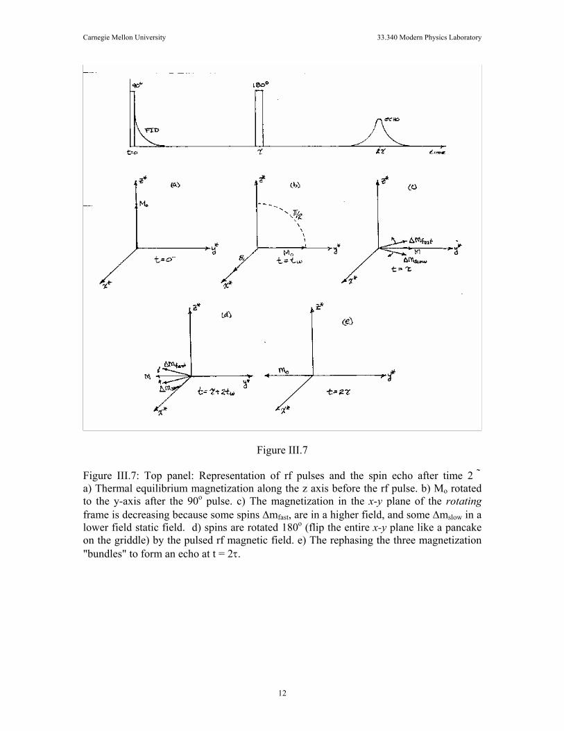
of living systems. For example, preliminary work has already shown that blood flowpatterns in both the brain and the heart can be studied without dangerous catheterizationor the injection of radioactive isotopes. MRI scans are able to pinpoint malignant tissuewithout biopsies, and we will see many more applications of this diagnostic tool in thecoming years. The scans rely on measuring the "T1" and "T2" values in various bodytissues: in this experiment you will learn what these are and how to measure them for asmall sample.

You will be using the first pulsed NMR spectrometer designed specifically for teaching.The PSI-A is a complete spectrometer, including the magnet, the pulse generator, theoscillator, pulse amplifier, sensitive receiver, linear detector, and sample holder. Manysubstances can be studied.

Now you are ready to learn the fundamentals of pulsed nuclear magnetic resonancespectroscopy. We recommend that for this laboratory experiment you proceed asfollows:

1) Read about nuclear spin and spin precession [start with Section III , below) soyou grasp the basic ideas.

2. Read the discussion in Section IV to become famil iar with the equipment.

3. Start a series of measurements as outl ined in Section V. Go as far as you canin the time available. Quality of results is more important than quantity.

II. BACKGROUND READII\G

Nuclear magnetic resonance is a vast subject. Tens of thousands of research papers andhundreds of books have been published on NMR. We will not attempt to explain or evento summarize this literature. An extensive annotated bibliography of imporlant papers andbooks onthe subject is provided atthe end of this section. The following references mayprovide additional useful background for the experiment and should be perused:

Reference

Melissinos2

Cohen-Tannoudji3

Sections

8.1 - 8.4.18.4.2 - 8.4.4F(rv)

Paqes

340-35936r-374443-45r

Topics

Magnetic Resonance basicsDetection (but not the MPL way)

Quantum vs classical descriptions

III. THEORY OVERVIEW J

J j

jU U B

z zU B m B mz zm j j j j jmz zm

U B o B

fBo "Relaxation" along the external field: NNNN

oUkT kTN e e

N

zM N N N N + N

oB BM N N

kT kT

Exercise 1: Derive Eq. III.12 from the preceding two equations

not

o zz M MdMdt T

Mz t T

z oM t M e

Phase decoherence of the spins with respect to each other: x-y

dJdt

dJBdt

dBdt

Exercise 2: Show that the precessional frequency, o, is just the resonant frequency in Equation III.7.

x-y create x-y

dM M Bdt

B

oB z x-y B t B t x B t y B z

rotating coordinate system effective field

B z rotating z B z

effB t B x B z

effdM M Bdt

x B t x B t x t y B t x t y

oB o oB

effB t B x

x z

x-y x-y z

net magnetization precessing about the constant magnetic field Bz in the x-y plane. Nothing Else! x-y B z x-y

x-y

wt

wt

wt B

x xdM Mdt T

y ydM Mdt T

t T

x y oM M e B z distributionx-y x-y

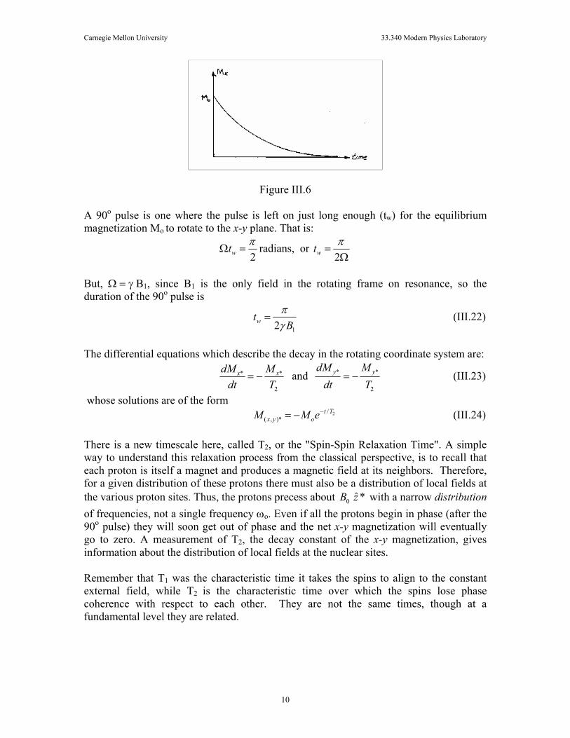
The need for pulse sequences: t rotatingx-y

Tx y oM t M e

x-y rotatingx-y

summarize o B

fBo

dM M Bdt

B t B t x B t y B z

effB t B x B z

o oB effB t B x

x-y

IV. EXPERIMENTAL EQUIPMENT

x-y

Do not move the carriage initially. Chances are it is already set at its "sweet spot" where the magnetic field is most uniform.

x-y This is the detector that you will use to record both the free induction decays and the spin echoes signals

V. EXPERIMENTAL PROCEDURE V.1 Learning to use the equipment:

x-y

V.2 Getting a FID signal and tuning the receiver circuitry x-y

V.3 Measuring T2

* for glycerin x-y z x-y z-

Carnegie Mel Ion Universi fy 33.340 Modern Physics Laboratory

direction. But this magnelrzation builds exponentially with a time constant, T1. EachMeasurement, that is, each pulse sequence, must wait at least 3 T1 (preferably 6-10 T1's)before repeating the pulse train. For a single pulse experiment that means a repetitiontime of 6- 10 Tr. If you chose pure water as a sample, with Tr = 3 sec, you would have towait a half a minute between each pulse. Since several adjustments are required to tunethis spectrometer, pure water samples would be very time consuming and difficult towork with. The effect of not fully recovering the z magnetization between pulse trains iscalled saturation.

Glycerin has a T1 of roughly 20 ms at room temperature. That means the repetition timee.rrr be set 100 urs and the magnettzation will be in thermal equilibrium at the start ofcach pulse sequence (or single pulse in this first experiment).

The actual shape of the Tr- is not exponential, but proportional to /,(O)/O, where ,/,(@)is the Bessel function of order I , @ : yGdt 12, d is the sample diameter, and G is thefield gradient dB, I dz. For now, simply characterrze the shape by its width:

Estimate T2* for glycerin by finding and recording the full-width at half maximum(FWHM) of the FID signal.

V.4 Quick First Estimate of the Spin-Lattice Relaxation Time, 71, .for glycerin.

The time constant that characterizes the exponential growth of the magnetization towardsthermal equilibrium in a static magnetic field, T1, is one of the most impoftant parametersto measure and understand in magnetic resonance. With the PSl-A, this constant can bemeasured directly and very accurately. It also can be quickly estimated. Let's stafi with anorder of magnitude estimate of the time constant using the standard glycerin sample.

1. Adjust the spectrometer to resonance for a single pulse free induction decay signal.

2. Change the Repetition Time, reducing the FID until the maximum amplitude of theFID is reduced to about 1/3 of its largest value.

The order of magnitude of Tr, is the repetition time that was established in step 2. Settingthe repetition time equal to the spin lattice relaxation time does not allow themagnetrzation to return to its thermal equilibrium value before the next 90o pulse. Thus,the maximum amplitude of the free induction decay signal is reduced to about l/e of itslargest value. Such a quick measurement is useful, since it gives you a good idea of thetime constant you are trying to measure and allow you to set up the experiment conectlythe first time.

V.5 Two-Pulse Zero-Crossing Method for T1

A two pulse sequence can be used to obtain a two significant figure determination of Tr.The pulse sequence is:

23

cannot detect x-y x-y just before the pulse V.6 A Better Two-Pulse Method for T1 x-y

V.7 Spin-Spin Relaxation Time - T2 for glycerin V.8. Two-Pulse Spin Echo Method x-y

tTV t V e

Camegie Mel lon Universi ty 33.340 Modern Physics Laboratory

exponential curve directly with a non-linear least-squares fitting algorithm. Make a goodT2 me&surement for glycerin using the two-pulse echo method. Measure the height of the

spin echo for enough values of r using the two-pulse echo method and extract a value(using a fit) for T2.

There are several issues, some inherent in the apparatus, some inherent in the physics,that can result in the data not lying on a straight line. These can be classified as:

1. 'Nonlinearities' in the detector response.2. Errors caused by improper use of the digital scope.3. The actual decay may not be exponential under the conditions of the two pulseexperiment, fot some samples.

They are discussed here:

1. The echo amplitude is to be measured by using the output of the rectifring detector,not the phase sensitive detector, because the latter can be subject to small but easilyobserved fluctuations and the relative phase ofthe reference and the signal are not under

,experimental control. However, the signal detection rectifier response is nonlinear at lowsignal levels due to 'noise'. This can be easily seen by examining an echo amplitude that

decays exponentially with t at high signal levels, but non-exponentially at low signallevels. One can go from one regime to the other just be changing the gain of the receiveramplifier. For our purposes, no signal less than about 0.4 volts should be used foramplitude measuremenls unless you include corrections for the detector nonlinearity.How to identify and compensate for this effect is an exercise left to the student. Discussit with the instructor.

2. In earher times, the limited sampling rate of digital oscilloscopes could cause aparticular illusion in what is seen called "aliasing". Beats in the FID signal at the scopesampling frequency will show up on the digital scope as a "flat" trace. If the spin echoesare too narrow, i.e.,too brief in time, then display of a chain of them on the digital scopewill result in large fluctuations in the apparent amplitude of each of them. That is becauseeach screen of the scope samples the input waveform only finite number of times. If theecho is too sharp for the sampling rate used it has information in a frequency rangeexceeding half the sampling rate. Fortunately, with present-day scopes this problemrarely shows up.

3. Physical diffusion of the spins in the sample: real physics. A spin randomly diffusesfrom one region to another in the sample. Since those regions have different staticmagnetic fields because of field inhomogeneity, the random movement will cause loss ofphase memory of the spins. That phase memory loss occurs at a more rapid rate thansimple exponential decay:

V( l :2r)=Vo € " i u-T

a = D(ydB,la)z l tZ

(v.2)where

26

(v 3)

DdB/dz t D V.9 Multiple Pulse Spin Echo Sequences for T2. independently

tTV t n V e e

Carnegie Mel lon Universi ty 33.340 Modern Physics Laboratory

Now measure T2 fbr glycerin using M-G pulse sequence. Compare this result with yourprevious result using the two-pulse method. Try to separate the effect of diffusion fromthe value of Tz.

V.l0 Better Estimate of Diffusion Effects

We can use the vadous pulse sequences to separate the spin-spin relaxation and diffusioneffects on the echo. If the time between the nl2 and the n pulse in the M-G sequence is t,the echoes occur at t":n(2r). From Equation V.2, using the fact that the echoes areequally spaced and the difference between any two is equal to t;2 c

_ t l

V(t, '1:V(t , - r ) e-at t r e ' t2

Recursive application of this relation gives

ar!v(t , :2nr) :v(0) e-"n" s "

If one uses a single pulse to create an echo at a time tn,lhen the required delay is nt, andthe echo heisht after that time is

, _, , 'Vr(t , ) :V(0) u-a(nr ' ' ) ' u 1'2

The ratio, R, of Equation (6) to Equation (7) is

R(t, =2nt) = n-a(nr-n)(r ' ) l (v 8)

Thus, a plot of ln(R) vs. (n3-n) would have a slope of cx tr3. Notice that T2 has canceledout. You now have a method to measure the effects of difTusion through the field gradientof the magnet, u:D(ydB/dz12ll2. Another test of the B pulse length being incorrect isthat the points in the plot of ln(R) vs. (tt'-n) will alternate around the best fit line drawnthrough them, a clear indication that the M-G sequence does indeed correct the error fromone pulse on the next pulse. Correct adjustment of the length of the B pulse will minimizethat alternation.

Use the two-pulse and the M-G measurements together to determine D(ydBldz)z forglycerol. Then consult the appendix "Estimating Field Gradients from Signal DecayShapes" to estimate dB ldz, and thereby obtain the diffusion coefficient D.

V.l l Examining water

Try this part of the lab only f you have successfully completed the previous parts.

Use the simple method described in Section V .4.2 to get an estimate of Tr for distilledwater. The full measurement would be tough. We can shoften the relaxation times byadding paramagnetic Cu** ions to the water. Why? A CuSO+ (cupric sulfate) solution hasbeen prepared. For this solution, measure Tr and then T2 using the two-pulse and M-G

(v.5)

(v 6)

(v 7)

29

V.12 Other Interesting Behavior Try this part of the lab only if you have successfully completed the previous parts. V.13 Magnetic Field Contours Try this part of the lab only if you have successfully completed the previous parts. x-y x-y

V.14 Rotating Coordinate Systems This part is easy and may help you grasp the way the spin vectors respond to the static and the rotating fields. is

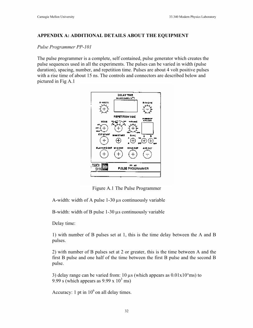
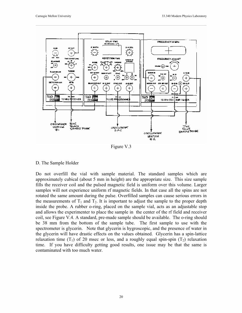
APPENDIX A: ADDITIONAL DETAILS ABOUT THE EQUIPMENT Pulse Programmer PP-101

Leave in during MPL experiments.

15 MHz OSCILLATOR/AMPLIFIER/MIXER:

IMPORTANT: DO NOT OPERATE THE POWER AMPLIFIER WITHOUT ATTACHING TNC CABLE FROM SAMPLE PROBE. DO NOT OPERATE THIS UNIT WITH PULSE DUTY CYCLES LARGER THAN 1%. DUTY CYCLES OVER 1% WILL CAUSE OVERHEATING OF THE OUTPUT POWER TRANSISTORS. SUCH OVERHEATING WILL AUTOMATICALLY SHUT DOWN THE AMPLIFIER AND SET OFF A BUZZER ALARM. IT IS NECESSARY TO TURN OFF THE ENTIRE UNIT TO RESET THE INSTRUMENT. POWER WILL AUTOMATICALLY BE SHUT OF TO THE AMPLIFIER IN CASE OF OVERHEATING AND RESET ONLY AFTER THE INSTRUMENT HAS BEEN COMPLETELY SHUT OFF AT THE AC POWER ENTRY.

15 MHz Receiver not

Auxiliary Components (not used in present MPL setup)

References Experiments in Modern Physics, Quantum PhysicsQuantum Mechanics Data Reduction and Error Analysis for the Physical Sciences, Books

Papers

Carnegie Mellon University 33.340 Modern Physics Laboratory

Estimating Field Gradients from Signal Decay Shapes

Last Revision: R. A. Schumacher March 2008 ver. 1.5

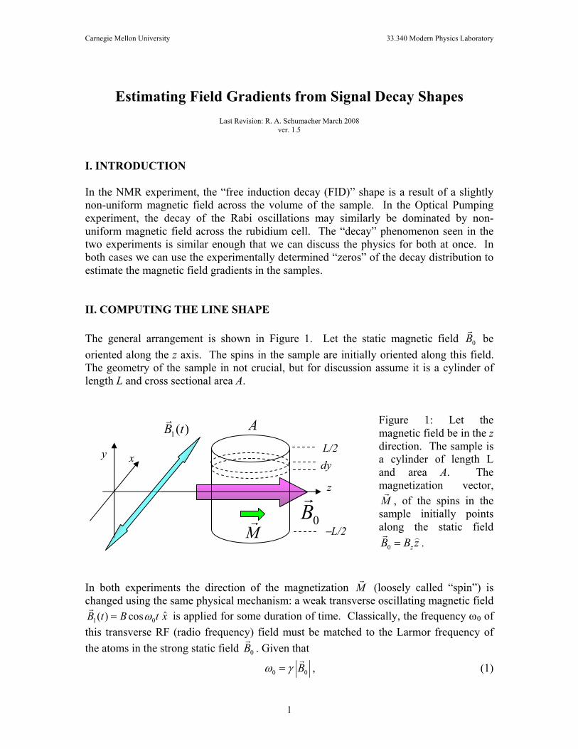
I. INTRODUCTION In the NMR experiment, the “free induction decay (FID)” shape is a result of a slightly non-uniform magnetic field across the volume of the sample. In the Optical Pumping experiment, the decay of the Rabi oscillations may similarly be dominated by non-uniform magnetic field across the rubidium cell. The “decay” phenomenon seen in the two experiments is similar enough that we can discuss the physics for both at once. In both cases we can use the experimentally determined “zeros” of the decay distribution to estimate the magnetic field gradients in the samples. II. COMPUTING THE LINE SHAPE The general arrangement is shown in Figure 1. Let the static magnetic field 0B be oriented along the z axis. The spins in the sample are initially oriented along this field. The geometry of the sample in not crucial, but for discussion assume it is a cylinder of length L and cross sectional area A.

Figure 1: Let the magnetic field be in the z direction. The sample is a cylinder of length L and area A. The magnetization vector, M , of the spins in the sample initially points along the static field

0 zB B z .

In both experiments the direction of the magnetization M (loosely called “spin”) is changed using the same physical mechanism: a weak transverse oscillating magnetic field

1 ˆ( ) cos 0B t B t x is applied for some duration of time. Classically, the frequency 0 of this transverse RF (radio frequency) field must be matched to the Larmor frequency of the atoms in the strong static field 0B . Given that

0 0B , (1)

z

y x L/2

L/2

dy

0B M

A 1( )B t

1

Carnegie Mellon University 33.340 Modern Physics Laboratory

where is the gyromagnetic ratio of the material under study, one can find the frequency if the field strength is known. In the NMR experiment, the frequency is near 15 MHz, while in the optical pumping experiment it is near 50 kHz. To measure a signal, in the NMR experiment we activate the oscillating field long enough to rotate the spins into the x-y plane, and then observe the net magnetization in this plane as a function of time. In the optical pumping experiment, we activate the oscillating field indefinitely, sending the spin angles through many full cycles of resonance, and observe the degree of opacity of the rubidium cell versus time using a photodiode detector. In the quantum mechanical picture, the Larmor frequency turns out to be related to the transition energy between the magnetic sub-states of the system. The splitting of the energies of the sub-states is caused the Zeeman Effect. That is, if the magnetic sub-states are separated by energy E , then we have 0E . This relationship between the quantum and classical pictures is not obvious at all, but comes from the study of spin and magnetic moments at the level of the Advanced Quantum Physics course. For this discussion, the classical picture is entirely sufficient. Now suppose that the static field 0 ( , , )zB B x y z z is not perfect, and that across the volume of the sample there are field gradients /zB x , /zB y , and /zB z . That is, in different locations in the sample the static field is slightly different, and hence the Larmor frequency is slightly different. Hence the spins precess about the static field at slightly different rates, and the coherence of the detected signal goes away after some characteristic time. That time is related to the strength of the field gradients and the size of the sample. The “line shape” of this loss of coherence is what we are calculating in this note. For definiteness, suppose the gradient /zB y is the only non-zero one we have to consider. Let the response signal of the detector to spins at location y1 be written 1( ) cosdS t Ady t1 , (2) and the response at a different location y2 be written 2 ( ) cosdS t Ady t2 , (3) where Ady are the separate differential volume elements across which the responses are detected. Ady is to be construed as proportional to the number of spins in the sample volume and also their net magnetization. The two y locations are not the same and can be a macroscopic distance apart. The combined response from these two locations is then 1 1 1( ) ( ) ( ) (cos cos )dS t dS t dS t Ady t t2 . (4) Using a trigonometric identity, this is the same as

2

Carnegie Mellon University 33.340 Modern Physics Laboratory

1 2 1 21 12 2

( ) 2 cos ( ) cos ( )dS t Ady t t . (5)

Even though the y locations can be a finite distance apart, we suppose that the frequency difference between them is still very small, so that we may write

1 2 1 2(zz

dB )B y ydy

. (6)

This equation assumes that the change in magnetic field strength across the sample is well characterized by a gradient and a separation. Put the origin at the center of the sample, and let the two locations in y be symmetric above and below y = 0, so that we have

1 2 2zdB ydy

. (7)

For each separation of the response locations specified by y, we must include a “weighting” factor to account for all possible ways we can have two places in a sample of length L separated by distance 2y. Since the sample of length L, the room within which we can place a segment of length 2y is L 2y. The dimensionless factor is taken to be (1 2y/L). We have also assumed that the spread in frequencies is so small that the bandwidth of the driving RF field is wide enough to “excite” the spins across the whole sample. If this were not the case, then only a sliver of the whole sample would respond to the oscillating magnetic field. Thus, we can define the average frequency to be equal to the driving frequency:

1 21 ( )2 0 . (8)

With these replacements we can write Eqn. (5) as

0( , ) 2 cos cos 1 2zdB ydS y t A t t y dydy L

. (9)

To determine the overall response of the detector to this range of oscillatory actions within the sample we must now integrate this expression over the height of the sample. To make the integral symmetric, we will take half the result of integrating from –L/2 to L/2. That is,

/2

0/2

( ) ( , ) cos cos 1 2L

z

L

dB yS t dS y t A t t y dy

dy L. (10)

Introduce, for convenience, the combination

3

t . - " .d8, ,K=y , l .ay

so that we can write, with the further substitution I = k y ,

s(r; = tas6,t1=

Carnegie Mel lon Universi ty

so that we have

L/2/ \e , . , l 12 I

Acos(a4r) J cos(@)[ 1-2; ]dy- t ,J \ L)

33.340 Modern Physics Laboratory

(11)

(r2)

(1 3)

(14)

The second integral vanishes because we are integrating an odd integrand over thesymmetric range from-Ll2to +L12. This line shape function S(t) can be rewritten in amore comDact form if we make the substitution

. . l r . I ? .= Acos(anr) ; lcos( i ) , l i + . lcos( i ) i d i

' " 'kr k ' J '

2sinkL: Acos(atnt\-- .2 + 0

IrL

.L dB-L(D(/)=k--v ' -1 .2 dy2

s(/) = AL cos(atot, sin@(r)

@(r)

This is our main result: it is the "line shape" of the detector response of a sample in whichnot all elements are oscillating at the same frequency. Note that the signal is proportionalto the sample volume AL, as one would expect. At time / : 0 the signal is just AL, as canbe seen from the first term of the Taylor expansion of the sine. The function sin (D / O isthe "sinc" function, which looks like a sine multiplied by a hyperbola. It has its first zero

when @ =Tt, and then a subsequent maximum near @:3n12. This is the feature we canexploit to estimate the size of the field gradient.

In reality, additional derivatives of B will besymmetric field of the PS-1A magnet,

nonzero. For the cyl indrical ly

dB,fdx : dB,,f dy : -G 12<0 and aB,fdz : G >0, where z

cylindrical sample, as in the present experiment, the free

V' B :0 impl ies thatis the symmetry axis. For a

induction envelooe is now

[1 s)^. . J,(vGdr12)M(r\ :2M^ ' "

" yGdr 12

where d is the sample diameter and ./,(x) is the Bessel function of order 1-. I t is

osci l latory but not periodic. To measure the gradient G, measure the t ime tcorresponding to the f irst zero of Jr(x), which occurs at approximately x = 3.83.This is most accurately measured using an echo, to el iminate uncertainty associatedwith preamp recovery t ime fol lowing a 90o pulse.