Chapter 3

Nuclear MagneticResonance Spectroscopy

3.1 Nuclear Spins

Nuclei may possess a spin angular momentum and the observation of nuclearspins in Stern-Gerlach type experiments played a large role in the developmentand acceptance of particle physics. The original Stern Gerlach experiment in1922 probed the electron spin in silver atoms evaporated in an oven and flyingthrough a magnetic field (Fig. 3.1).

Ag, (700º C)

N

S

Figure 3.1: Stern and Gerlach observed the quantized electron spin νz = ± 12· geνB

in a beam of neutral silver atoms.

Silver atoms have 47 electrons, (electronic shell: 1s22s22p63s23p64s24p63d105s1).The single outer electron was expected to have zero angular momentum (l=0)

1

2 CHAPTER 3. NUCLEAR MAGNETIC RESONANCE SPECTROSCOPY

Nucleus Abundance Spin Spin projections γN (107 1T ·s )

1H 99.98% I= 12 mI = ± 1

2 26.75213C 1.11% I=1

2 mI = ± 12 6.727

14N 99.64% I=1 mI = 0,±1 1.93319F 100% I= 1

2 mI = ± 12 25.177

31P 100% I= 12 mI = ± 1

2 10.840

Table 3.1: Nuclear spins regularly used for NMR spectroscopy.

and no interaction with the magnetic field was expected. The experiment, how-ever, showed two discreet trajectories indicating a quantized magnetic propertyof the atoms. Both, the presence of an inherent electron spin, and its quantizedproperty in an external magnetic field came as a surprise and affected the de-velopment and wide acceptance of quantum physics. Nuclear spins are about 3orders of magnitude weaker and were later observed in similar experiments. Theobservation of nuclear spins gave first indications that nuclei have structure.

Nuclei are composed of protons and neutrons, both of which have inherentspins of I = 1

2 . Hence, nuclei with an odd number of protons or neutrons musthave a spin I6=0; if the sum of protons+neutrons is odd, then the spin must bea half-integer number I = n + 1

2 (n=0,1,...). The nuclear spin quantum num-ber I for nuclei commonly encountered in nuclear magnetic resonance (NMR)spectroscopy is shown in table 3.1.

EmISpin state energy

γN gyromagnetic momentB0 Magnetic fieldmI spin projection

EmI= −γN~B0mI (3.1)

In absence of a magnetic field, the nuclear spin is not an observable property.In presence of a magnetic field B0, the nuclear spin adopts quantized valuesmI = -I, -I+1 ... -I, which explains the discreet trajectories observed in theStern-Gerlach experiments. There exists no classical interpretation for the spinquantization. The energy of the spin states in a magnetic field can be calculatedusing the nuclear gyromagnetic moment γN in table 3.1 using the equation 3.1.

Nuclear Spin Signals

The energy difference ∆E = γN~B0 between proton spin states in a strongmagnetic field of 1 T can be directly estimated as ∆E = 2.675 · 108~s−1 cor-responding to a frequency of 42.6 MHz. This so called ”Larmor frequency” isdirectly proportional the the magnetic field strength. Irradiation of a sample

3.2. NMR SPECTRA 3

with the Larmor frequency of its nuclei will lead to spin excitation and absorp-tion of the radiation.

1H gyro. moment γN = 2.7 · 108 1Ts

Magnetic field B0 = 1.0 T

Planck constant ~ = 1.05 · 10−34 Js

Boltzmann const. k = 1.4 · 10−23 J

KTemperature T = 300 K

NαNβ

= exp

(−γN~B0

kT

)NαNβ

≈ 1− 6.7 · 10−6

(3.2)MHz and GHz frequencies are comfortably in the range of radiowave emitters

and detectors, so spectroscopic characterization is straightforward. Original ex-periments used a fixed frequency radiowave oscillator and observed absorptionwhile scanning the magnetic field strength induced by electromagnetic coils.The size of the observed signal is proportional to the population difference be-tween the lower (α) and upper (β) spin state, and to the energy per absorbedphoton (the latter is directly proportional to B0). We can use the Boltzmanndistribution as shown in equation 3.2 to estimate population differences. Withthe approximation that e−x ≈ 1 − x for small x, the population difference isalso proportional to B0, and we find that the signal depends quadratically onthe field strength. This explains the the great efforts to obtain ever strongermagnetic fields for NMR and the early adoption of superconductor materials inthe corresponding magnetic coils. Modern NMR spectrometers operate at fieldstrength up to 20 T.

3.2 NMR Spectra

Chemical Shift

When an external magnetic field is applied to a sample, not all nuclei feel thesame field strength. The electron spins with their much higher magnetic momentget spin polarized and induce a local magnetic field which can shield the nucleusor increase the field at the nucleus (Fig. 3.2). Both, the nuclear polarizationand the electron polarization are proportional to the magnetic field, thereforethe shielding effect leads to a frequency shift which is a constant fraction of theresonance frequency. It is therefore advantageous to plot NMR spectral shiftsas parts per million (ppm) on a proportional scale δ = ν−ν0

ν0· 106, invariant to

the field strength of a particular experiment.The discovery of the chemical shift moved the investigation of nuclear spins

into the domain of chemistry, whereas originally such investigation were of in-terest only to nuclear physicists who wanted to get insight into the structureof atomic nuclei. In 1952, only 6 years after the publication of the first NMRspectra, Bloch and Purcell were awarded the Nobel Prize in Physics for their

4 CHAPTER 3. NUCLEAR MAGNETIC RESONANCE SPECTROSCOPY

Bel=-σB0

B0Bloc=B0-σB0

( ) 012

BN σπ

γν −=

Figure 3.2: The applied magnetic field B0 interacts with the electron angular momen-tum and induces a magnetization Bel. This magnetization affects the local magneticfield acting onto the nucleus and shifts the corresponding resonance frequency ν.

work. Through the direct measurement of local magnetic fields, the nuclearspins are perfect probes for local electronic structure. Nuclear spins are alwaysreported relative to a chemical standard, typically tetramethyl-silane (TMS) toremove the need for an absolute calibration. Chemical shifts for some chemicalgroups are shown in figure 3.3.

δhigher ν

012345678

(TMS)

SiCH3CH3

CH3

CH3R

OH

RH

H

H

H

HR

H

H

R

R

HRR O

OH

91011

RN

H

H

O HR

Figure 3.3: Chemical shifts for a number of chemical groups. Electron withdraw-ing groups ”deshield” the protons and lead to smaller shifts and higher excitationfrequencies.

Spin-Spin Coupling

Beyond the interaction with the electron angular momentum, nuclear spins alsointeract with other nuclear spins leading to the so called ”fine structure” or J-Jsplitting. This interaction can increase, or reduce the energy of a spin state by

3.2. NMR SPECTRA 5

14J. If we consider a system of two coupled spins A and X, then the combinedsystem can be in an αAαX , αAβX , βAαX , or βAβX state. The excitation energyof either spin from αAαX in the example in Fig. 3.4 is reduced by 2 · 1

4J , butthe excitation energy from αAβX or βAαX to βAβX is increased by 2 · 14J . Theexcitation energies for the nuclear systems A and X are therefore now split intotwo lines and split by exactly the same energy ± 1

2J = J .

uncoupled spins

αA

βA

αα

αββα

+¼ J

-¼ J

αX

βX

+¼ Jcoupled spins

+¼ J

-¼ JαX

βX

αA

βA+¼ J

uncoupled spins

hνX +½ JhνA +½ J

hνA - ½ J hνX - ½ JhνA

hνXhνA

hνX

ββ

Figure 3.4: Coupled versus uncoupled spin system: Uncoupled spins A and X canbe excited independently, e.g. first A, then X (left) or first X, then A (right). In thecoupled system, the spins can stabilize (αβ, βα) or destabilize (αα, ββ) each other by14J , leading to a splitting of each transition line.

Nuclear spins are magnetic dipoles and spin-spin interaction therefore falls ofvery rapidly, proportional to 1

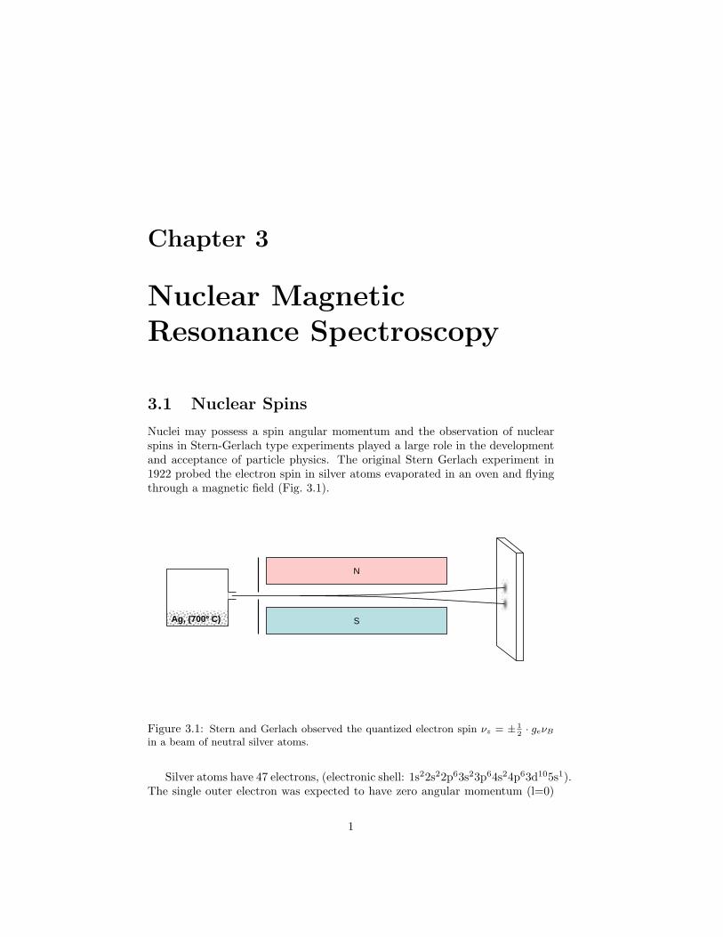
r6 . Through-space interaction is therefore limitedto very short ranges (< 5A), and the spins couple most strongly through theelectronic system. The coupling through bonding electrons is illustrated in Fig.3.5: The Fermi coupling between nuclear and electronic spin in a single atomleads to a preferentially antiparallel alignment of nuclear and electronic spin.According to Pauli, the two electrons in the bonding orbital to a neighboringatom must be of opposite spin, carrying the spin information to the next atom.The Hund rule indicates that electrons in different orbitals preferentially adoptthe same spin state, carrying the spin correlation into further bonds. However,through-bond spin coupling is is quickly decreasing with the distance, i.e. thenumber of atoms between the nuclei.

The JJ splitting is independent of the magnetic field ( 6= chemical splitting)and is usually given in Hertz (Hz). Typical coupling constants for a number ofvicinal (neighboring) and geminal (non-neighboring) JJ-interactions are givenin Figure 3.6. JJ Coupling across more than 3 (for JHH) or 4 (for JCH) bondsis rarely observed.

When a spin is coupled to two identical spins (e.g. in a system R-C(H)=CH2),then two identical splittings lead to the observation of a triplet with intensityration of 1:2:1 with identical spacing of J. If a spin is coupled to two different

6 CHAPTER 3. NUCLEAR MAGNETIC RESONANCE SPECTROSCOPY

hydrogen

Fermicoupling

Paulirule

Fermicoupling

H

H

CC

ethyleneHund rule

H He- e-

Figure 3.5: Coupling of nuclear spins occurs predominantly via the electronic system.The Fermi coupling, Pauli’s rule and Hund’s rule determine whether parallel spins(e.g. hydrogen) or antiparallel spins (e.g. ethylene) are lower in energy.

spins x and y, then the interaction will lead to a splitting by Jx and another byJy and therefore result in 4 lines of equal intensity for the single spin. The finestructure can become very convoluted if multiple couplings are present (e.g. 18lines in the spectrum of CH3-CH2-CH2-NO2), complicating the analysis.

Spin-spin coupling also occurs through space, but the magnetic dipole-dipoleinteraction falls off with the 6th power of the distance. Therefore only inter-actions across small distances are observed and no discreet splittings can beassigned. However, the through space coupling of spins A and B reduces theintensity of both spin signals. The intensity of spin A can be recovered by sat-urating the transition for spin B. This effect is called the ”Nuclear Overhauser”effect and allows to characterize through-space coupling.

Spin decoupling

To interpret convoluted spectra, it would be desirable to observe only selectedJJ couplings which can be unambiguously assigned. This can be done by irra-diating the sample with a continuous, strong RF pulse at the Larmor frequencyof a chosen spin x. The selected spin will undergo multiple spin flips due toabsorption and stimulated emission. If the spin flips occur mich faster than thecoalescence time, then the neighboring spins will interact with a time-averagedspin 1

2α + 12β = 0, hence the splitting with spin x is removed. All other spins

still couple, so the missing couplings can be assigned to interaction with spin x.

3.3 Fourier Transform NMR

Instead of sweeping the magnetic field B0 for a constant RF frequency ωf , orsweeping ωf for constant B0, it is possible to excited multiple spins coherentlyand to observe the temporal evolution of the induced magnetization. To excitemultiple transitions, the excitation pulse must contain all the correspondingfrequencies. A short pulse always contains many frequencies (remember theuncertainty principle: ∆E∆t ≥ ~) and can be considered to be the superposition

3.4. NMR IMAGING 7

R

R' HH

H

RRH

R R

H

RR

H H

RH

RH

HR

R

JHH = 12..15 Hz 6..8 Hz 6..9 Hz

H

R

H

R

JHH = 0-3 Hz 13..18 Hz7..12 Hz

R

R' HR

1JCH = 125..200 Hz

RH

H

160 Hz

R H

250 Hz

R

R3C HR R2C

H

HRC H

2JCH = -2 ..-5 Hz -2.5 Hz 40-66 Hz

R

R3CCH3

RH

HR3C

R

HR3C

3JCH = 4 ..8 Hz 7-13 Hz 3 Hz

Figure 3.6: Selection of typical homonuclear JHH and heteronuclear JCH couplingconstants.

of discrete frequencies. The creation of such RF pulses is no major challengeand is illustrated in Fig. 3.8.

If a large ensemble of spins interacts with the electromagnetic field, thenthe superposition of particle waves will resemble a classical particle and insteadof quantized properties and a probabilistic description of transitions, we canconsider the motion of a quasi-classical particle. We therefore discuss the exci-tation and observation of a ”spin wavepacket” in the ground (α) and excited (β)state and talk about the total magnetization as if it were a true property of thesystem. In the x-y plane, the external field leads to a torque

−→T = −→µ ×

−→B0 on

the magnetization vector. If the field is oriented along the z-axis, this results ina spinning of the magnetization (superposition of the magnetic moments) in thex-y plane with the difference frequency between α and β, the Larmor frequency.For easy interpretation, the total magnetization

−→M =

∑i

−→µi is considered and

plotted as shown in Fig. 3.9. The rotating magnetization vector induces currentsinto a detector coil, i.e. emits electromagnetic radiation which can be detected.

3.4 NMR Imaging

Imaging in one Dimension

The resonance (Larmor) frequency for a spin transition is proportional to themagnetic field strength: µL = ( γ2π · B0. If a field gradient B = B0 + x · Bx isapplied along one axis, then the resonance frequency is a linear function of thespin positions within the sample. A NMR spectrum will then directly measurethe spin density along the selected spatial coordinate and offer a one-dimensional

8 CHAPTER 3. NUCLEAR MAGNETIC RESONANCE SPECTROSCOPY

image of the sample. Please note, that possible frequency shifts due to chemicalshift and fine-structure are very small and are ignored. Measuring multipleone-dimensional projections along different axes allows to reconstruct a two- orthree-dimensional image as shown in Fig. 3.10.

All biological tissue contains water and other proton sources, hence the con-trast of 1H NMR for biological imaging may be unsatisfactory. But a secondobservable is directly available: the T2 spin relaxation time which is a sensitiveprobe to diffusion properties, pH, proton mobility, and other factors. T2 is pref-erentially measured in the time domain using a π −mixing − time− π/2 pulsesequence as shown in Fig. 3.11. Because signals measured with the π − π/2pulse sequence may show different phases for spins with long/short τ1 lifetimes,selection of a suitable mixing time can give excellent contrast in imaging exper-iment and allows the easy distinction of different types of biological tissue asseen in the T2 enhanced brain image in figure 3.14, center.

Imaging in Multiple Dimensions

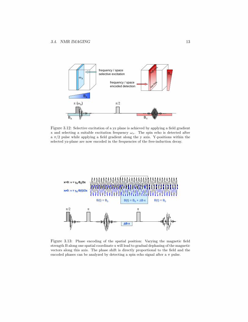
If imaging is performed in the time domain, multiple pulsed field gradients canbe used to mark spins in more than one dimension. In a first approach, we canexcite only a selected slice of the sample along axis x with a field gradient Bx anda frequency selective excitation pulse. After free induction decay is complete, aπ pulse leads to a spin echo, which is detected while applying a field gradientBy. The detected frequencies thus encode the y position within a slice x, asshown in Fig. 3.12.

There is, however, a more elegant way for multidimensional imaging: adetected coherent spin signal is due to the larmor precession of the correspondingspin magnetization vector sin(ω ·t+δ0) with the larmor frequency ω = γN ·B0. Ifa field gradient B0(x) = B0 +x ·∆Bx is applied, the Larmor frequency will varyas a function of x. As illustrated in Fig. 3.13, the precessing spins now dephasewith time t by ∆ω · tx = γN · B0(x) · tx. After the field is switched off, we canobserve the unperturbed frequencies, but with a phase shift of δ0 = δ0 +∆ω · tx.A measurement of the phase shift is therefore a direct measurement of theposition along the axis x. In a sequence of spin-echo measurements, multiplephase shifts can be induced along different axes using field gradients Bx, By andBz to obtain 3-dimensional spatial information.

Instead of discrete field gradient pulses along x,y and z, is is preferable touse sinusoidally varying B-fields Bx,y,z ∼ sin((ax + by + cz) · t). The corre-sponding frequency components a, b and c are superimposed on the actual spinfrequencies and can be recovered by the fourier transform. This allows the mea-surement of three-dimensional images in a single experiment, but requires thatthe experiment can resolve the applied frequency components from linewidtheffects.).

3.4. NMR IMAGING 9

Medical Imaging

The potential use of NMR tomography in medicine was a large motivator fromthe early days of NMR imaging. NMR tomography offers a non-invasive andnon-destructive imaging method for biological tissue which easily penetrates ahuman body. As compared to X-ray tomography, NMR offers unique capabilitiesbeyond the simple imaging of tissue density. First and foremost, we shouldconsider the spin relaxation time τ1, which is easily measured with a schemeas shown in 3.11. The spin relaxation time is a function of rotational mobility(e.g. high in water, low in fat), pH (≥ 7 in normal cells, often lower in cancercells), and diffusion. The contrast can therefore be optimized for a particulardiagnostic problem. With spin lifetimes of seconds, it is even possible to followthe flow of fluids. Figure 3.14 shows the image of a brain after a stroke, usingdifferent imaging methods to diagnose the blood flow or lack thereof in theaffected brain regions (1).

The ability to observe blood flow and metabolic activity resulted in a novelmedical field, the so called ”functional imaging” or fNMR, where local brainactivity is monitored and correlated with mental activity. Fig. 3.15 showstwo examples, the brain activity associated with moving a finger and the moreabstract brain activity of imagining pain (1, 2). These methods offer unprece-dented insight into neurological processes.

Direct spectroscopic measurements can characterize metabolites and prop-erties such as pH (via analysis of phosphate signals). In some cases, metabolicpathways can be followed, such as the chemical pathway of drugs.

10 CHAPTER 3. NUCLEAR MAGNETIC RESONANCE SPECTROSCOPY

©1999 W

illiam R

eusch, All rights reserved,

http://ww

w.cem

.msu.edu/~reusch/V

irtualText/Spectrpy/spectro.htm

#contnt

7.2 Hz

δ 1.02

triplet

7.5 Hz

δ 4.35

triplet

7.5 Hz

δ 2.04

quadruplet7.2 Hz

triplet

Figure 3.7: Example for spin decoupling in the molecule 1-nitropropane: The convo-luted band at δ2 appears to be a sextet. Decoupling at the frequency of the δ1.02 band(bottom) reveals a triplet due to coupling with the CH2NO2 group. Decoupling of theband δ4.35 leads to a quadruplet due to coupling with the CH3 moiety (second fromtop). The apparent sextet is therefore due to 12 lines, which cannot be experimentallyresolved.

3.4. NMR IMAGING 11

Figure 3.8: 5 Sinusoidal pulses with frequency differences of approximately π/10 (top)and their sum (bottom). The sum is an apparently shorter pulse, and indeed we expecta frequency uncertainty according to the uncertainty principle (h∆ν ·∆t ≥ h).

x

y

zB0

μi

Μ

x

y

zB0

μi Μπ/2zy pulse

Figure 3.9: Nuclear spins µi and total magnetization M =∑µi in a magnetic field

B0 (left), and after excitation of a coherent spin wavepacket with a(π2

)zy

pulse.

12 CHAPTER 3. NUCLEAR MAGNETIC RESONANCE SPECTROSCOPY

ωL

ωL

ωL

Bo B o

Bo

Figure 3.10: NMR Zeugmatogram: If a linear magnetic field gradient B0 is appliedalong an axis, then the spin frequencies ωL in the sample are directly proportionalto the position along the axis. The NMR spectrum then measures spin density asfunction of position. Measuring multiple projections along different axes allows thereconstruction of an image (Lauterbur 1973, Nobelprice for medicine together withMansfied in 2003).

xy

zB0

Μ

xy

z

π

xy

z

xy

z

t1 π/2τ1 short

τ1 long τ1 long

τ1 short

Figure 3.11: Measurement of τ1: after spin inversion with a π pulse, waiting timet1 allows for spin relaxation. With a π/2 pulse, spins are turned into the x-y planefor detection of the free induction decay (FID) signal. Signals which decayed by morethan 50% have opposite sign of the magnetization vector before the π/2 pulse andhave opposite phase in the FID.

3.4. NMR IMAGING 13

ωX

π (ωX) π/2

BY

BX BY

BX

frequency / spaceselective excitation

frequency / spaceencoded detection low

freq.

high f

req.

Figure 3.12: Selective excitation of a yz plane is achieved by applying a field gradientx and selecting a suitable excitation frequency ωx. The spin echo is detected aftera π/2 pulse while applying a field gradient along the y axis. Y-positions within theselected yz-plane are now encoded in the frequencies of the free-induction decay.

x=0: ν = γN⋅B0/2π

x≠0: ν = γN⋅B(t)/2π

B(t) = B0 + ΔB⋅xB(t) = B0 B(t) = B0

π/2 ππ

ΔB⋅x

Figure 3.13: Phase encoding of the spatial position: Varying the magnetic fieldstrength B along one spatial coordinate x will lead to gradual dephasing of the magneticvectors along this axis. The phase shift is directly proportional to the field and theencoded phases can be analyzed by detecting a spin echo signal after a π pulse.

14 CHAPTER 3. NUCLEAR MAGNETIC RESONANCE SPECTROSCOPY

Copyright ©1999 BMJ Publishing Group Ltd.Prichard, J. W et al. BMJ 1999;319:1302

Figure 3.14: Magnetic resonance images after clinical stroke (blocked blood vesselsin the brain). Left: ”Diffusion weighted imaging” shows damaged tissue. Center: con-ventional T2 weighted image. Right: Magnetic resonance angiography (measurementof blood flow) shows flow void in blood vessels.

Cop

yrig

ht ©

1999

BM

J P

ublis

hing

Gro

up L

td.

Pric

hard

, J. W

et a

l. B

MJ

1999

;319

:130

2

P.L

. Jac

kson

et a

l., N

euro

psyc

holo

gia

44, 7

52–7

61 (

2006

).

Figure 3.15: (A) Functional NMR image of the brain during finger movement showsincreased blood flow to particular brain regions. (B) fNMR imaging of the brain duringthe abstract thought about pain.

Bibliography

[1] J.W. Prichard, J.R. Alger, ”The NMR revolution in brain imaging”, BMJ319, 1302 (1999).

[2] P.L. Jackson, E. Brunet, A.N. Meltzoff, J. Decety, ”Empathy examinedthrough the neural mechanisms involved in imagining how I feel versushow you feel pain”, Neuropsychologia 44, 752761 (2006).

[3] P.C. Lauterbur, ”Image Formation by Induced Local Interactions: Exam-ples Employing Nuclear Magnetic Resonance”, Nature 242, 190 (1973).

[4] T.F. Budinger and P.C. Lauterbur, ”NMR Technology for Medical Stud-ies”, Science 226, 288-298 (1984).

[5] P.J. McDonald and B. Newling, ”Stray field magnetic resonance imaging”,Rep. Prog. Phys. 61, 1441 (1998).

[6] W. Kckenberger, ”Nuclear magnetic resonance micro-imaging in the inves-tigation of plant cell metabolism”, Journal of Experimental Botany 52, 641(2001).

[7] K. Wtrich, ”NMR Studies of Structure and Function of biological maro-molecules”, Nobel price lecturehttp://nobelprize.org/nobel prizes/chemistry/laureates/2002/wuthrich-lecture.html.

[8] L. Frydman, ”Single-scan multidimensional NMR”, C. R. Chimie 9, 336(2006).

[9] A. Mittermaier and L.E. Kay, ”New Tools Provide New Insights in NMRStudies of Protein Dynamics”, Science 312, 224 (2006).

[10] S.F. Keevil, ”Spatial localization in nuclear magnetic resonance spec-troscopy”, Phys. Med. Biol. 51, R579 (2006).

[11] J.P. Hornak, ”The Basics of NMR”,http://www.cis.rit.edu/htbooks/nmr/inside.htm.

[12] B. Jaun, ”Script Analytical Chemistry IV”,http://www.jaun.chem.ethz.ch.

15