Nuclear magnetic resonance in magnetic systems and metals

Nuclear magnetic resonance in magnetic systems and metals

Denis Arčon

University of Ljubljana, Faculty of mathematics and physics, Slovenia

Institute “Jozef Stefan”, Ljubljana, Slovenia

1

Motivation

2

Solid-state physics: - Crystal structure and lattice dynamics, - Electronic properties, - Magnetism, (anti)ferroelectrics, multiferroics - Superconductors

Local probes that would be simultaneously sensitive to lattice as well to electrons

Experimentalists toys: Scattering techniques: - XRD - Neutron diffraction Measurements of macroscopic properties: - Dielectric spectroscopy, - Magnetization measurements

(SQUID, … ) - Specific heat, thermal

conductivity, thermal dilatometry, …

Vibrational spectroscopies

So, why NMR?

3

Nuclear magnetic resonance (NMR) A TOOL to study condensed matter systems o Local, microscopic, site‐specific probe o Virtually all elements are NMR active o study electronic spin structure, lattice

structure

o Non‐invasive – no current, no contacts on the sample

o ωNMR ≈ 0 (μeV), gives partial q information (cf. neutron diffraction)

o can be combined with other techniques: transport, magnetization, dielectric, optical, …

o IJS laboratory: extreme conditions: low temperatures, high pressures, different magnetic fields up to 9.34 T

Elvis is alive and well, working as an NMR spectroscopist in Ljubljana.

Magnetic resonance - basics

4

History: Purcell (NMR in paraffin), Bloch (NMR in H2O), Zavoisky (EPR) Magnetic resonance phenomena is found in systems that poses magnetic moments and we are “in tune” with a natural frequency of the magnetic system. Magnetic resonance technique offers a high resolution experimental probe for the study of static and dynamics properties of local magnetic fields. Nuclear magnetic resonance (NMR): typically in the 10-500 MHz range Electron paramagnetic resonance (EPR): typically in the 1-100 GHz range NMR is utilized widely not only in physics and/or chemistry but also in medical diagnostics (MRI) and so on. ・Physics Condensed matter physics ・Chemical Analysis and/or identification of material ・Biophysics Analysis of Protein structure ・Medical MRI (Magnetic Resonance Imaging)

„It‘s lupus, do the MRI!“

Outline

5

Lesson Subject

1 Introduction to magnetic resonance; Bloch equations, relaxation times, dynamics susceptibility

2 The basic spin Hamiltonian for NMR

3 Hyperfine coupling interaction, Knight shift

4 The Moriya theory of spin-lattice relaxation

5 NMR in the superconducting state (just briefly)

6 NMR in the magnetically ordered state

7 Examples: fullerides, pnictides and quasi-1D magnetoelectric system


6

Nuclear magnetic moments: A system such as nucleus may consist of many particles coupled together so that for a given state the nucleus possesses a total magnetic moment m related to a total angular momentum G Here g is a scalar called gyromagnetic ratio and is typical for nuclei or electrons. Simple model: m = iS = ipr2 ; G=mvr=m(2pr/T)r ; i=e/T g = e/2m g thus decreases with increasing particle mass

Γ

gm =

γ [MHz/T ] ν [MHz]

proton 2.675102 42.58 B0 [T]

electron 1.759105 27990 B0 [T]

QM: II Nˆˆˆˆ gm ==G


7

Nucleus γ/2π

(MHz/T)

1H 42.576

2H 6.53566

3He -32.434

7Li 16.546

13C 10.705

14N 3.0766

15N -4.3156

17O -5.7716

23Na 11.262

63Cu 11.284

65Cu 12.109

51V 11.193

31P 17.235

129Xe -11.777

Magnetic moment in the external magnetic field

• Torque on the magnetic moment:

• Change of the angular momentum

8

BT

= m

Bdt

dB

dt

Γd

== mgm

m

Larmor precesion m

0BNL g =

Larmor frequency Typically in the rf range up several houndred MHz

Effect of rf field • But, in order to see precession, we first need to shift

magnetization away from the z-axis. This is the job of rf pulses.

• In the rotating frame, that rotates with Larmor frequency L, m is static Beff=B0- L/g=0.

• rf field B10cos(Wt) = BR+BL

• Rotation around the xR axis

9

0=R

effB

m

xR rfB

90o pulse tWgB10=p/2

yR

B10 of the order of 10 mT


10

Quantum mechanics: we have to treat m and G as operators.

IIΓ nn

ˆˆˆˆ

gm ==

In an applied field, Example: I = ½ (case of 1H or 13C for instance)

0ˆ

a B=B z → , 1, , 1,Im I I I I=

ZZ IBBH ˆˆˆ0

gm ==

mBBE Zm 00 gm ==

In the MR we attempt to detect the splitting of these energy levels by appropriate perturbation. The interaction must be such, that the angular frequency matches the splitting: LARMOR FREQUENCY

0BEL g ==

Which perturbation will trigger the transitions between these levels? R.f. irradiation perpendicular to B0 will do the job!

tIBH Lxrfrf g cosˆ=


11

Time dependent Schrödinger equation has the general solution in the form We can now calculate the expectation value for mz, for instance

ZHt

i ˆ=

=m

tiE

mImmeuc/

,

)()(

ˆ'

)(ˆ)(*

22

21

2/1

*

2/12/1

*

2/1212/1

*

',

/)(*

''

bacccc

cmc

mImecc

dtt

I

m

mm

mm

z

tEEi

mm

zz

mm

==

=

=

=

=

gg

g

g

tmm

Normalised WF: 2

2/1

*

2/1

2

2/1

*

2/1 & bccacc ==


12

The calculation for the expectation value for mx, is slightly more complicated, but follows the same steps By recalling we can derive

=

=

',

/)(*

'ˆ'

)(ˆ)(*

'

mm

x

tEEi

mm

xx

mImecc

dtt

mm g

tmm

1,)1()1(,ˆ

1,)1()1(,ˆ

=

=

mImmIImII

mImmIImII

gm

gm

=

=

tab

tab

y

x

0

0

sin

cos

)( 22

21 baz = gm

Magnetic resonance – basics spin-lattice relaxation

13

N-

N+

= NWNW

dt

dN

Simple rate equations

Fermi golden rule: p

= bbab EEaVbP2

ˆ2

WWWbVaaVb ==

22

ˆˆ

If we introduce n=N+ -N- and N=N+ +N- then N+=½(N+n) and N-=½(N-n) then we get

WtentnWndt

dn 2

0)(2 ==Initial difference in energy population will exponential decay to zero!


14

Problems: 1. Absorbed power dE/dt=N+WħωL-N-WħωL=WħωLn(t) will also vanish after some time

(not supported by the experiments). 2. What if W = 0 (no perturbation) and we change magnetic field (MZ should change,

what is not predicted by this equation)! Therefore, there MUST be a process that allows the system to accept (or release) the

magnetic energy. It is the coupling to the lattice spin-lattice relaxation Thermal equilibrium: difference in the population given by the energy difference

TkBTkE BB eeN

N0

0

0g

==

= NWNWdt

dN

In thermal equilibrium d/dt=0 TkB BeWW 0/g

=


15

Why now WW? Rate equations are solved by introducing n and N and we get In terms of magnetization, this actually reads as

Spin Lattice

)(

)()(

1

)()(

0

1

1

0

=

==

WW

WWNnWW

T

T

nnWWnWWN

dt

dn

0

1

zzM MdM

dt T

=


16

Spin-lattice relaxation also solves the problem of absorption of r.f. energy. Namely, if we take into account external perturbation (described by W) and spin-lattice relaxation together, then we derive In the steady state And the absorbed power will be

1

02T

nnWn

dt

dn =

1

021

1

WTnn

=

1

021 WT

WnnWdt

dE

==

0 2 4 6 8 10

0.0

0.2

0.4

0.6

0.8

1.0

P/P

S

2WT1

Magnetic resonance – basics Bloch equations

17

Classical description of the motion of magnetic moments in external magnetic field Torque due to the action of B0

This torque will change the angular momentum In addition we have also relaxation phenomena to return back to equilibrium. We define two relaxation times T1 – spin-lattice relaxation time and T2 – spin-spin relaxation time to allow longitudinal and transverse magnetizations to come back

0B

m

000 BMdt

MdB

dt

dB

dt

d

===G

gmgm

m

0

2

x xy

dM MB M

dt Tg=

0

2

y y

x

dM MB M

dt Tg=

0

1

zzM MdM

dt T

=

Please note that changes in Mx and My do not change the magnetic energy


18

Bloch equations in compact form

==

1

2

2

00

/100

0/10

00/1

T

T

T

RMMRBMdt

Md

g

With initial conditions

2/

0cost T

xM t m e t=

00 , 0 0,x y zM m M M M= = =

we have solutions in the form

2/

0sint T

yM t m e t=

1/

0 1t T

zM t M e

=

0 5 10 15

-2

0

2

Mx, M

y (

arb

. u

nits )

time

Mx

My


19

The application of rf field perpendicular to the static magnetic field will thus lead to an extra transverse magnetization. In a typical experiment, the rf field will be linearly polarized (along the x-axis)

xlab xrot

yrot ylab

t

The result of previous calculations is that, we can write Mx component of the magnetization in the laboratory frame as We thus defined a complex r.f. susceptibility with components

1sin''cos'sincos)( BtttMtMtM rot

y

rot

xx ==

''' i=

2

2

2

0

200

2

2

2

0

2020

0

1

1

2''

12'

TT

T

TT

=

=

Rotating frame with field

Stat

ion

ary

solu

tio

ns

dM

/dt=

0


20

When the detection coil is filled with measured material, its inductance changes by

L=L0(1+) The complex impedance of the coil thus also changes as Z=R+iL=R-L0’’+iL0’ The real part of Z changes by R/R=L0’’/R=Q’’ In unperturbed coil, the relation between the magnetic energy and the current producing that magnetic field is ½L0i0

2= ½B12V/m0

Because of change in the impedance, the average dissipated power is In MR experiments we are thus measuring ’’. But ’ is related to ’’ through Kramers-Kronig relations, so we in principle know both of them. Also, please note that P is proportional to 0 so it can provide a quantitative information about the static magnetic susceptibility of the samples!

''2

1

2

1 2

1

0

2

0 m

VBRiP ==

Magnetic resonance – basics Method of moments

21

The experimentalists thus measure the absorption ’’(). The theorists tend to be more familiar with the Green functions or time-correlation functions of spin operators. In a linear response theory, developed for MR by Kubo and Tomita, ’’() is expressed as A time evolution of Mx operator is calculated in the interaction representation Lets define the spectral lineshape as If we perform inverse FT of the above expression, we can derive

dteMtMTk

V ti

xx

B

= 0ˆˆ2

''

/ˆ/ˆ ˆˆ tHi

x

tHi

x eMetM =

dteMtM

Tk

Vf ti

xx

B

== 0ˆˆ2

'')(

p

defMtMTk

V ti

xx

B

= )(2

10ˆˆ

2


22

If we look at the above expression at time t=0, then we notice the following Therefore <Mx

2> is a measure for the area under the resonance curve. But, if we take the time derivative and then take its value at t=0, we can make even a step further The n-th time derivative will be thus

p

dfMMTk

Vxx

B

= )(2

10ˆ0ˆ

2

p

dfiMtMdt

d

Tk

Vtxx

B

= = )(2

10ˆˆ

20

p

dfi

MtMdt

d

Tk

V n

n

txxn

n

B

= = )(2

0ˆˆ2

0

3

)1(ˆˆˆˆ

ˆˆ

222

312

,

2

,

2

,

,

====

=

IIiziyixi

i

xix

gmmmm

mm


23

We can thus define n-th moment of the resonance as Let us calculate the second moment of the the line Taking the above expression at t=0 and slightly rearranging terms, we finally derive

2

0

ˆ

0ˆˆ

)(

)(

x

txxn

n

n

n

n

M

MtMdt

d

i

df

df=

==

0ˆˆ,,1

0ˆ)ˆˆ(0ˆ0ˆ

/ˆ/ˆ

2

/ˆ/ˆ/ˆ/ˆ

2

2

x

tHi

x

tHi

x

tHi

xx

tHi

x

tHi

x

tHi

MeMHHe

MeHMMHedt

diMeMe

dt

d

=

=

2

2

2

2

2

ˆ

ˆ,1

)(

)(

x

x

M

MH

df

df

==

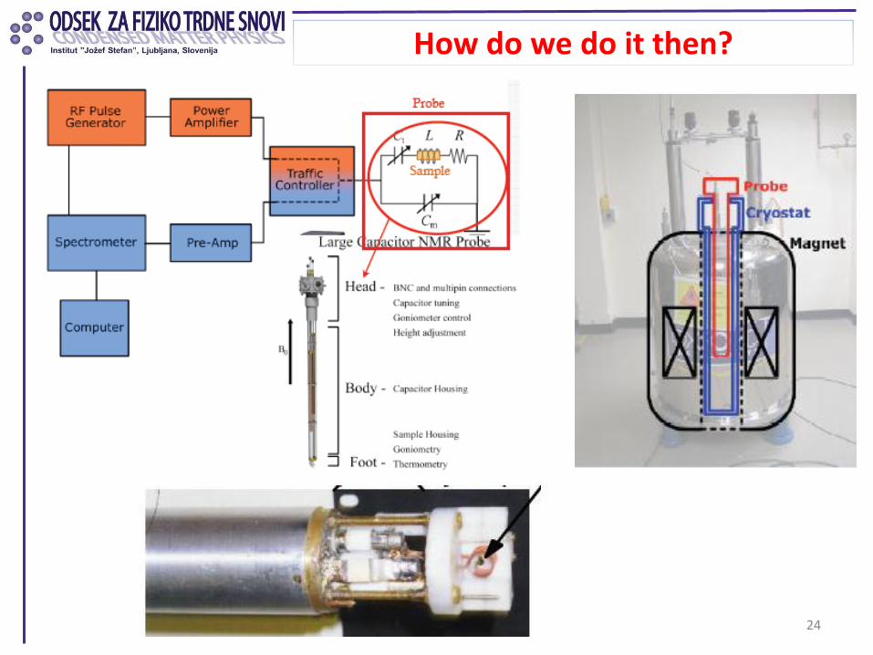
How do we do it then?

24

Current Piston-cylinder cell for NMR

• for pressures up to 20 kbar

• large sample volumes (< 200 mm3)

• easy to manufacture

• inexpensive materials

• dangerous

clamp/screw (Be-Cu)

bottom piston (Be-Cu)

body (Ni-Cr-Al)

upper piston (Ni-Cr-Al)

Magnetic resonance – basics pulses

26

If we can neglect the effect of relaxation times (typically this is justfied when the duration of rf fields is short compared to T1 and T2), then one can also show that the effect of rf field will be to rotate the magnetization

After p/2 pulse we observe FID

Small current induced in the coil is amplified and then analyzed

Magnetic resonance – spin echo

27

When FID is to short to be observed then we may want to try with spin echo

Measurements of relaxation times

28

Magnetic resonance – what we have learnt so far?

29

1. Classical Bloch equations (torque + T1 + T2) 2. T1 processes must result in a transfer of energy since it involves magnetic

dipoles reorienting in a magnetic field. Quantum mechanically, it is a change of populations between spin-down states to spin-up states which are nondegenerate in a magnetic field. Since the energy is typically gained by the lattice, T1 is termed as the lattice or longitudinal spin relaxation time.

3. QM treatment in the Schrödineger and Heisenberg picture 4. In magnetic resonance we are measuring the imaginary part of the r.f. spin

susceptiblity ”(). 5. Method of moments:

1. O-th moment M0=f()d is proportional to the static spin susceptibility 2. Higher moments are in fact given by the commuators [H’, Ix]. In

particular we emphasized the first moment M1= f()d / M0, which is just the center of the resonance and the second moment M2= (-M1)2 f()d / M0 which is measure for the linewidth.

Magnetic resonance – a brief summary after first lectures

30

Bloch equations in compact form Magnetic resonance measures Method of moments

==

1

2

2

00

/100

0/10

00/1

T

T

T

RMMRBMdt

Md

g0 5 10 15

-2

0

2

Mx, M

y (

arb

. u

nits )

time

Mx

My

dteMtMTk

V ti

xx

B

= 0ˆˆ2

''

B0

Brf

2

22

0

2

0

2

0

0

ˆ

ˆ,'1

)(

)(

ˆ

ˆˆ,'1

)(

)(

x

x

x

xx

M

MH

df

df

M

MMH

df

df

=

=

=

=

NMR observables

31

NMR = local, real-space probe where the behaviour of nuclear spins can be monitored on a site-to-site basis. Types of NMR observables: 1. NMR spectrum is fundamental and major element of sample

characterization • Width & distribution

Sample quality Crystallographic inequivalent sites Local site disorder

• NMR shifts, which are measured as a frequency shift proportional to the applied field is a fundamental measure of the various terms in spin Hamiltonian. In magnetic systems is a measure of local spin susceptibilities. Various sources: s-contact shift (in metals = Knight shift) Core-polarization shift Dipolar shift Chemical shift

2. NMR dynamics as represented by the spin-lattice relaxation time T1. T1 is linked to “(q,) via the fluctuation-dissipation theorem.

1100

==

g

resres

B

NMR – basic Hamiltonian

32

Nuclear magnetic moments in solids constitute nearly perfect example of an ensemble that is weakly coupled to its neighborhood. In NMR we attempt to explore this weak coupling to measure sample’s static and dynamic properties. General spin Hamiltonian 1. Zeeman term

NMR: detect the transitions between these levels. It is usually the strongest term and in most experiments it will range between 10-500 MHz.

neQdipZ HHHHH =

ZZ IBH ˆ0g=


33

2. Dipolar term It is much weaker than Zeeman term as it is at most in the several 10 kHz range. It will

give rise to a Gaussian type of broadening of resonances with a second moment Calculated from the definition of the second moment

=

ji ij

ijjiji

ij

ji

dipr

rIrI

r

IIH

,53

22 ˆˆ3ˆˆ

2

g

=

ji ij

ij

rNII

,6

22

242)1cos3(1

)1(4

3 g

2

2

2

2

0

2

ˆ

ˆ,1

)(

)(

x

xdip

M

MH

df

df

=

=

NMR – dipolar interaction; example

34

2. Dipolar term Effect of molecular motions: we need to Take a time average over the dipolar term

=

ji ij

ij

rNII

,6

22

242)1cos3(1

)1(4

3 g

)1cos3( 2 ij

Nuclei of spin I 1 have electric quadrupole moment.

2

,

3

6 2 1 2Q

eQH V I I I I I

I I

=

Q > 0

Q > 0 for convex (egg shaped) charge distribution.

,

1

3!QH V Q

= 23 k k k

k protons

Q e x x r

=

Wigner –Eckart Theorem:

2

0

VV

x x

=

=

r

Quadrupole term: zzeq V=

223 1

4 2 1Q

e qQE m I I

I I =

Ref: C.P.Slichter, “Principles of Magnetic Resonance”, 2nd ed., Chap 9.

zzeQ I I Q I I=

Q in field gradient

=

2222

2)1(ˆ3

)12(4IIIII

II

qQeH ZQ

Axial symmetry: =(Vxx-Vyy)/Vzz

Quadrupole Interaction


36

Some comments about the Quadrupole term: 1. It is frequently the leading (perturbation) term in NMR when I1/2. It is not

unusual to find it in the several 10 MHz range. In fact in some experiments we deliberately switch off magnetic field and observe only the transitions between the quadrupole split levels (Nuclear Quadrupole Resonance).

2. For I=1/2 the nuclear quadrupole moment Q vanishes identically according to the Wigner-Eckart theorem.

3. The choice made in the above equation is such that the principal axes fo the EFG tensor are chosen in such a way that |Vxx|<|Vzz|<|Vzz|. That is, |Vzz| is the largest principal value.

4. The symmetry plays an important role. For instance in cubic symmetries because of V=0 we see that Vxx=Vzz=Vzz=0. In other words, in this case HQ=0! However, even in cubic structures, strains can play a role as they effectively give rise to some distribution of Q. Then due to the first order broadening only the central transition -1/2<->1/2 will be resolved.

5. In tetragonal or trigonal symmetries we find that Vxx=Vyy or =0! We have an axially symmetric EFG.

Quadrupole interaction

37

Case of =0

)12(2

3)1(

2

1 2

312

0

==IhI

qQeIImhmBE QQm g

Quadrupole frequency

L+Q

L

L-Q L+Q L-Q L

First order satelites

)1cos3( 2

21 = QL nFor q 0:

Quadrupole interaction – powder lineshape

38

In case of powder samples with uniform distribution of q over the unit sphere, the first order transitions give rise to an intensity distribution between L+nQ and L-½nQ with a square root singularity at L-½nQ

)1cos3( 2

21 = QL n

m is no longer strickly a good quantum number so there are a second order frequency shifts. Interestingly they cancel out for the satelite transition, but they give a second order shift

)1cos9(sin4

3)1(

16

22

2

)2(

21

=

II

L

Q

L

I = 3/2

Quadrupole interacation - example

39

bcc lattice: only a single intercalation site

fcc lattice: Octahedral (O) and tetrahedral (T) sites

133Cs I=7/2 7/25/2, 5/23/2, …, -5/2-7/2)

fcc: site symmetries for the two Cs sites are 23 and m-3 => EFG=0

bcc: site symmetry (-4m.2) => =0

-5000 0 5000 52.3 52.4 52.5

SIM

bcc phase

133Cs

Inte

nsi

ty (

arb

. u

nit

s)

- ref

(ppm)

fcc phase

133Cs

Inte

nsi

ty (

arb

. u

nit

s)

(MHz)

O

T

T'

Electron-nuclear interaction

40

The coupling between the nuclear and electron moments can be divided into three contributions

hf

dip

nelne HHHH =

Chemical shift:

3/ rlIgH Bl

= mg … is the interaction to the electron orbital moment

and is usually contained in the so-called chemical shift in materials where the angular momentum is quenched. If this is the case, then the extra magnetic field at the nuclear site, which is a result of the orbital moment of the electrons, is expressed as

0BIHCS

= g

=

zzzyzx

yzyyyx

xzxyxx

Dimensionless second-rank tensor

0

0

=

Shift:

Chemical Shift

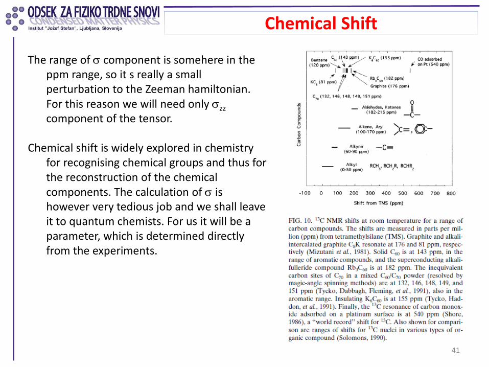
41

The range of component is somehere in the ppm range, so it s really a small perturbation to the Zeeman hamiltonian. For this reason we will need only zz component of the tensor.

Chemical shift is widely explored in chemistry

for recognising chemical groups and thus for the reconstruction of the chemical components. The calculation of is however very tedious job and we shall leave it to quantum chemists. For us it will be a parameter, which is determined directly from the experiments.

Chemical Shift – powder spectrum

42

Zeeman + Chemical shift Hamiltonians ij<<1 Principal axes system

0)1( BIH

= g

)1()1(0 zzLzzB g ==

=

zz

yy

xx

00

00

00

'

x’

y,y’

z’ x’

q

q

Axial symmetry xx=yy

1' = yy RR


43

The zz component, which we are looking for is The resonance frequency this reads To calculate the spectrum

2

|| cos =zz

)cos1( 2

|| = L

)]1(),1([)1(2

.

cos2

.

cos

.

cos.

||

||

||

=

==

=WW=

LL

LL

L

constf

const

d

d

constf

dconstdgdf

Presence of motions: can average the CS anisotropy even in powders


44

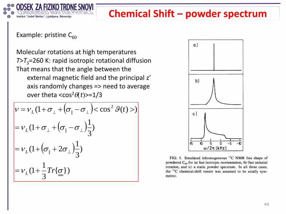
Example: pristine C60 Molecular rotations at high temperatures T>TS=260 K: rapid isotropic rotational diffusion That means that the angle between the

external magnetic field and the principal z’ axis randomly changes => need to average over theta <cos2qt>=1/3

}){3

11(

)3

121(

)3

11(

))(cos1(

||

||

2

||

Tr

t

L

L

L

L

=

=

=

=


45

Example: pristine C60

Electron-nuclear interactions cont.

46

We mentioned that the angular momentum interaction will give rise to a temperature independent chemical shift. However, in paramagnetic solids we need to take into account also the interaction between the electron and nuclear spins. When they are separated in space, then we can always count on the el-nuclear dipolar interactions

This will hold well also for p- and d-state electrons. For them we can in fact rewrite the

above equation in terms of a coupling traceless tensor T For p-electrons the spatial averaging gives the components

=

ji ij

ji

ij

ijjiji

B

ne

dipr

IS

r

rIrSgH

,35

2ˆˆˆˆ3

mg

0

2 ˆBTIgH B

ne

dip

= mg

SSr

Tr

T 33||

1

5

21

5

4==


47

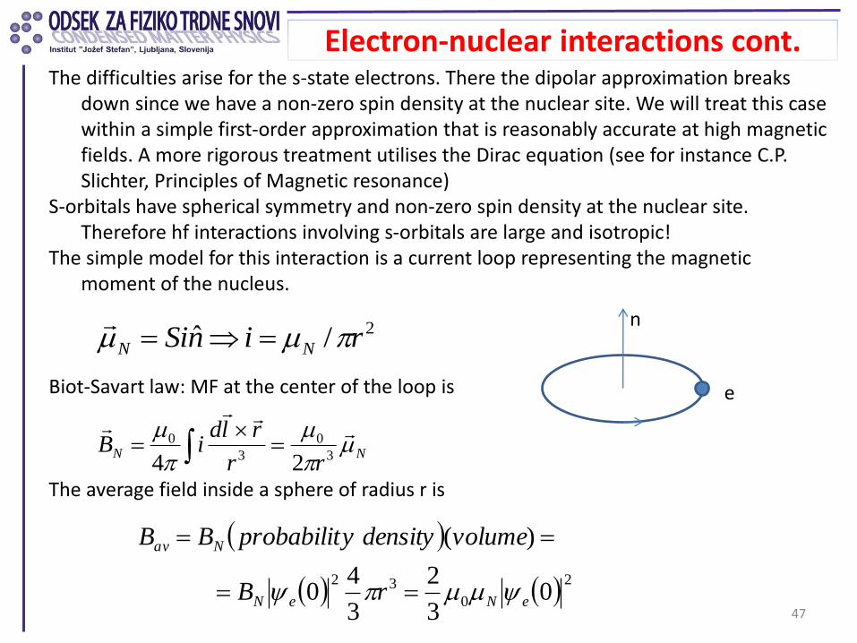
The difficulties arise for the s-state electrons. There the dipolar approximation breaks down since we have a non-zero spin density at the nuclear site. We will treat this case within a simple first-order approximation that is reasonably accurate at high magnetic fields. A more rigorous treatment utilises the Dirac equation (see for instance C.P. Slichter, Principles of Magnetic resonance)

S-orbitals have spherical symmetry and non-zero spin density at the nuclear site. Therefore hf interactions involving s-orbitals are large and isotropic!

The simple model for this interaction is a current loop representing the magnetic moment of the nucleus.

Biot-Savart law: MF at the center of the loop is The average field inside a sphere of radius r is

e

n 2/ˆ rinSi NN pmm ==

NNrr

rldiB m

p

m

p

m

3

0

3

0

24=

=

2

0

320

3

2

3

40

)(

eNeN

Nav

rB

volumedensityyprobabilitBB

mmp ==

==


48

The energy of the electron magnetic moment in this field will be Lets take 1s WF to get The more general treatment would actually give the famous Fermi contact interaction

SIaSIgBE eBave

===

2

0 03

2gmmm

Brr

B

e er

r/

3

1 =

p

rB=5.29·10-11 m

T5076.003

2/

2

01 == eBs ga gmm

rSIgH Bhf

32

3

8gm

p=

More formalistic calucaltion: see J.D. Jackson, Classical Electrodynamics, Ch. 5

Core-polarization hf coupling

49

d-electrons: Do we expect Fermi contact hf interaction (zero spin density)? They will frequently lead to the anisotropic hf interactions, which can be generally written as We may thus define the Knight-shift tensor with component

The result may be at first sight surprising since d-WF vanishes at the nuclear site. However, d-electrons can interact indirectly by polarizing core electrons. The Coulomb repulsion drives core s-states (fully occupied) closer to the nucleus. However, because of the Pauli principle “down-spin” s-orbitals will shrink more than “up-spin” s-orbitals. This will create a total negative hf field at the nuclear site. The associated fields can be in fact quite substantial sometimes. For Mn2+ in MnF2 it can be as large as -127 kOe/mB.

==

=zyxi

ii

B

i

zyxi

iii BIg

aSIaH,,,, m

i

B

iii

g

aK

gm 2=

Hyperfine interaction

50

What will Fermi contact inetraction do in magnetic systems? Since we expect that the electron spin dynamics will be fast on the time-scale of NMR

experiments (over 10 ms) we can take average of e- spin operator ||B0

rSIgH Bhf

32

3

8gm

p=

0BgN

AI

gAISAISIA

BAn

SZn

B

ZZZZ

mg

g

m

m==

hfnlocnn BBB == 0gg

=i

iihf SAB Hyperfine tensor: - on-site: Fermi contact, A= very strong and

known - Transferred: A can be anything - Dipole: A can be calculated, usually very weak; it

vanished in sites having cubic symmetry

S

BAn gN

AK

mg =

Units of A found in the literature: - A/ [s-1] - 10-3 A/gn [kG/spin] - 10-3 A/gng [kG/mB] - A/1.60210-12 [eV]


51

How do we extract hyperfine tensor?

Temperature (K)

0 50 100 150 200 250 300

Ma

gn

etic s

usce

ptib

ility

, (1

0-3

em

u m

ol-1

)

0.0

0.5

1.0

1.5

2.0

2.5

3.0

x = 0

x = 0.35

x = 0.5

x = 0.75

x = 1

0 50 100 150 200 250 300

0

-100

-200

-300

-400

-500

-600

13

3K

, 8

7K

(ppm

)

Temperature (K)

O-site

T-site

0.8 1.0 1.2 1.4

0

-100

-200

-300

-400

-500

-600

13

3K

O,T (

ppm

)

105 K

105 K

300 K

30 K

SQUID

(10-3 emu/mol)

300 K

133KO,T=133CS,O,T+(133aO,T/NAmB)

133CS,O = 15(8), 133CS,T = 148(15)

133aO = -2.28 kOe/mB, 133aT = -1.35 kOe/mB


52

But, be carefull! NMR is still a local real-space probe! Example, doping of Haldane chain system

89Y NMR Y2BaNi0.95Mg0.05O5

Tii

i THTH /1

1

1e1

=

valence bond solid with a single valence bond connecting every neighboring pair of sites

the ends of the chain behave like spin S=1/2 moments even though the system consists of S= 1 only

F. Tedoldi et al., PRL 1999

//upload.wikimedia.org/wikipedia/commons/6/6e/AKLT_GroundState.png

Knight shift

53

C60 versus K3C60

In metals: -The shift is always (almost) positive -The shift is very nearly temperature independent -The shift in principle increases with the nuclear charge Z.

The fact that metals have a weak spin-paramagnetism suggest that the shift may simply represent the pulling of the magnetic flux into the metal. However, the susceptibilities are to small to account for such effect. Knight postulated that the shift arises because of the interaction of nuclear spins with the conduction electrons through the s-state hf interaction.

Knight shift

54

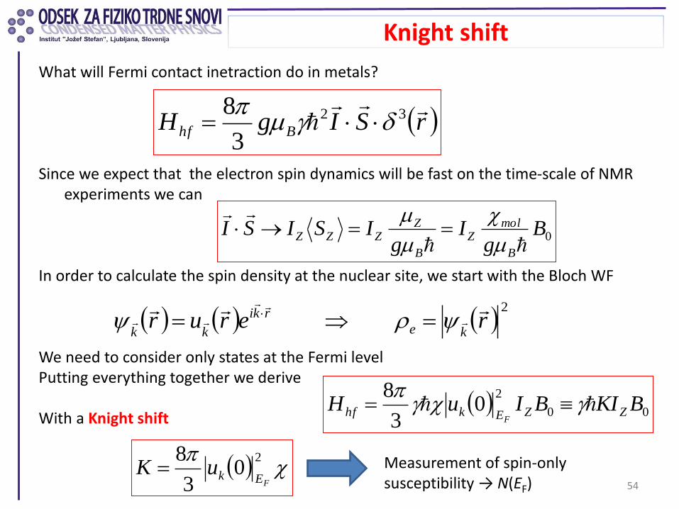
What will Fermi contact inetraction do in metals? Since we expect that the electron spin dynamics will be fast on the time-scale of NMR

experiments we can In order to calculate the spin density at the nuclear site, we start with the Bloch WF We need to consider only states at the Fermi level Putting everything together we derive With a Knight shift

rSIgH Bhf

32

3

8gm

p=

0Bg

Ig

ISISIB

molZ

B

ZZZZ

m

m

m==

2

rerurke

rki

kk

==

00

20

3

8BKIBIuH ZZEkhf

F

ggp

=

p 2

03

8

FEkuK = Measurement of spin-only susceptibility → N(EF)

METALLIC/SC STATE TMIT , TSC dependence pressure/doping

55

700 720 740 760 780 8000

40

80

120

160

200

RbxCs

3-xC

60

13

C Tc

133

Cs Tc

13

C TMIT

133

Cs TMIT

____________

susc. TMIT

XRD TMIT

SUPERCONDUCTOR

T (

K)

Cs3C

60

13

C Tc

133

Cs Tc

13

C TMIT

133

Cs TMIT

V / C3-

60 (A

3)

AFI

METAL

INSULATOR

MIT line is not vertical

Thinking about CC explanation dp/dT=S/V If the magnetic entropy (calculated per C60) is S = kB ln [S(S+1)] = kB ln 2. Structural study: V = 4 Å3 per C60

We thus estimate dp/dT = kB ln 2/V = 1.4·106 Pa/K Experimental value: dp/dT = 0.6 GPa/150 K = 4·106 Pa/K.

0 2 4 6 8 10 12 14 160

40

80

120

160

200

T (

K)

Cs3C

60

13

C Tc

133

Cs Tc

13

C TMIT

133

Cs TMIT

p (kbar)

NMR TMIT vs p diagram

Superconducting state

56

0 50 100 150 200 250 300120

140

160

180

200

220

M1 (

pp

m )

T (K)

15.5 kbarTc

chemical shift

aiso

S

Superconducting state

0

SCS χB

B

N

a

BA

=

m

demagnetization due to the Meissner screening currents and is in general not known

SCS χδδ A=

After subtraction of two shifts

CSCSCS δδ =

BANaaA m /

=

1.0 1.5 2.0 2.5 3.00.01

0.1

1 13

C - 87

Rb

13

C - 133

CsO

133

CsO -

87Rb

No

rma

lize

d S

pin

Su

sce

ptib

ility

Tc/T

2/kBTc=4.7(3)

Summary of interactions

57

neQdipZ HHHHH =

ZZ IBH ˆ0g=

=

ji ij

ijjiji

ij

ji

dipr

rIrI

r

IIH

,53

22 ˆˆ3ˆˆ

2

g

=

2222

2)1(ˆ3

)12(4IIIII

II

qQeH ZQ

0BIHCS

= g

0

2 ˆBTIgH B

ne

dip

= mg

rSIgH Bhf

32

3

8gm

p= i

B

iii

g

aK

gm 2=

Example - Pnictides

(La3+O2–)+(FeAs)–

Ba2+(Fe2As2)2– Li+(FeAs)–

Se atom has one extra electron compared to an As atom, Se2+: (4s)2(4p)6 As3-: (4s)2(4p)6

Chu et al., Nat. Phys. 5, 788 (2009)

Phase diagrams

59

Chu et al., Nat. Phys. 5, 787 (2009) SC: superconducting AFI: AFM insulating SDW: spin density wave

1. AFI phase next to SC is a hallmark of electron correlations. Correlations are strong and onsite.

2. No symmetry change through MIT! 3. Charge versus pressure controle of SC!

4. No disorder caused by the doping (off stoichiometries ...) 5. 3D vs 2D! 6. Importance of cubic symmetry!

Also see our papers Science 323, 1585 (2009) Nature 466, 221-225 (2010) Phys. Rev. B80, 195424 (2009)

Example: NMR in magnetically ordered state SDW in pnictides (1111 phase)

Cruz et al., Nature 453, 899 (2008)

Yildirim, arXiv:0804.2252

Fully frustrated

The frustration is lifted by a structural distortion

•SDW order with Q=(p,p) for 2a x 2a due to the interband nesting between the hole - and electron -bands •magnetic moments ~ 0.3 mB

75As coupling to Fe moments i

i

iAsB m

= =

4

1

A

=

=

=

=

zzyzxz

yzyyxy

xzxyxx

zzyzxz

yzyyxy

xzxyxx

zzyzxz

yzyyxy

xzxyxx

zzyzxz

yzyyxy

xzxyxx

aaa

aaa

aaa

aaa

aaa

aaa

aaa

aaa

aaa

aaa

aaa

aaa

43

21

;

;

AA

AA75As

a

b

3

1

4

2

Fe1 Fe2

Fe3 Fe4

Symmetry considerations: mirror reflection with respect to bc plane

AF phase – taken from LaOFeAs data Q = (1, 0, 1) Fe magnetic moments are aligned along the a−axis μFe ~ 0.3μB

cFexzAs eaB ˆ4 = m

cos1 0int

2

0int0 BBBBBBeff =

ONLY OFF-DIAGONAL TERMS!!!!

PM phase: 0HM

=

04 Baxx =

ONLY ISOTROPIC PART!!!!

Example: NMR in magnetically ordered state SDW in pnictides (1111 phase)

Example: NMR in magnetically ordered state

-10 -5 0 5 10

Inte

nsi

ty (

arb.

un

its)

80 K

180 K

-ref

(MHz)

NdOFeAs T phase: As reside on the 2c (1/4, 1/4, z) position, which is axially symmetric. = (Vxx-Vyy)/Vzz = 0 Q = 3 eVzzQ/ 2I(2I−1) =11.8 MHz NdFeAsO0.85F0.15

Q = 12.8 MHz

comparison (LaO0.9F0.1FeAs: Q = 11 MHz)

Low-T orthorhombic phase: As is on 4g (0, 1/4, z) position, =0.102

ONSET OF LOCAL MAGNETIC FIELDS

PHYSICAL REVIEW B 79, 094515 2009

EFG mainly originates from As 4p Electrons with a prolate p electron distribution in agreement with the negative Vzz.

g ,, )2()1(

1 QQeffAsmm B =

Axz=10.5 kOe/mB

large anisotropic hyperfine fields → experimental evidence for the Fe 3d and As 4p hybridizations

‘111’ family

LiFeAs

M.J. Pitcher et al., Chemical Communications 5918 - 5920 (2008).

NaFeAs

D.R. Parker et al., PRL 104, 057007 (2010).

Bulk superconductor

SDW below TSDW = 45 K

They are isostructural

23Na (I = 3/2) NMR in NaFeAs

52.5 53.0 53.5

293 K

80 K

75 K

70 K

65 K

60 K

55 K

50 K

45 K

40 K

35 K

30 K

12 K

23Na NMR, Na

1FeAs

[MHz]

52.2 52.4 52.6 52.8 53.0 53.2 53.4 53.60.0

0.5

1.0

1.5

2.0

2.5

Sig

nal In

tensity (

arb

. u

nits )

Frequency ( MHz )

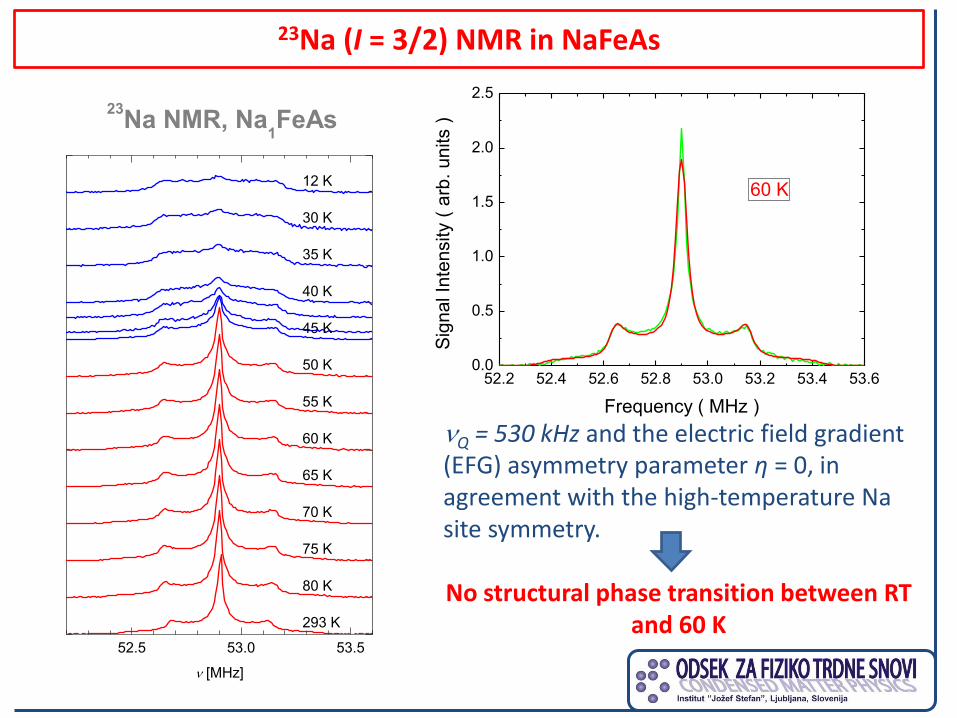
60 K

Q = 530 kHz and the electric field gradient (EFG) asymmetry parameter η = 0, in agreement with the high-temperature Na site symmetry. No structural phase transition between RT

and 60 K

23Na (I = 3/2) NMR in NaxFeAs

52.6 52.8 53.0 53.2

52.5 53.0 53.5 0 100 200 3000

50

100

150

300 K

(MHz)

Na1FeAs

Na0.9

FeAs

Na0.8

FeAs

(b)

Na1FeAs

Inte

nsity (

arb

. u

nits)

(MHz)

60 K

30 K

(c)

(a)

Na1FeAs

Na0.9

FeAs

Na0.8

FeAs

Wid

th (

kH

z)

T (K)

They are isostructural! Na vacancies in Na-deficient samples are expected to result in the local disorder and thus broadened NMR lines, which is in contrast to the measured 23Na central transition linewidth in the temperature range 50 − 300K Na+ migration??

Lineshape broadening is a clear indication of SDW transition. Variation of SDW order paramater with x. Still single line so NO phase segregation in this case.

Klanjšek et al., PHYSICAL REVIEW B 84, 054528 (2011)

Incommensurate SDW vs. other solutions

Commensurate SDW Commensurate SDW order with large local amplitude variations in the vicinity of the dopant Curro et al (2010).

INCOMMENSURATE SDW

-1 0 1 2 3 -1 0 1 2 3

a x = 0

Inte

nsity (

arb

. u

nits)

-ref

(MHz)

300 K

170 K

140 K

130 K

120 K

BA

36 K

38 K

41 K

43 K

50 K

120 K

130 K

140 K

300 K

170 K

x = 0.15b

-ref

(MHz)

NdOFeAs; P. Jeglič, PRB 2009

-5 -4 -3 -2 -1 0 1 2 3 4 5

Frequency ( MHz )

Bint = B0 sin α with α ∈ [0, 2π] and B0 = 0.45 T ordering vector (1/2− ϵ,0,1/2) for ϵ → 0

-6 -4 -2 0 2 4 6

Na1FeAs

- ref

(MHz)

Inte

nsi

ty (

arb

. u

nits

)

75As NMR

IC SDW amplitude of x=1 0.28μB x=0.9 0.04μB

x=0.8 0.13μB

75As (I = 3/2) NMR in NaxFeAs for T<TSDW: Nature of the order?

-6 -4 -2 0 2 4 6 4 5 6

c-SDW

dis-SDW

inc-SDW

= 0

0

Na1FeAs

- ref

(MHz)

In

ten

sity (

arb

. u

nits)

40 K

50 K

70 K

- ref

(MHz)

Still no structural phase transition, but some distribution due to local inhomogeneities

Structural phase with low-temperature tetragonal phase between 60 K and TSDW

THE MAGNETIC ORDER IS INCOMMENSURATE!!!

Klanjšek et al., PHYSICAL REVIEW B 84, 054528 (2011)

LiFeAs – 75As NMR

-2 -1 0 1 2

0 100 200 300

20.821.021.221.4

1.0 1.5

Inte

nsi

ty (

arb

. u

nit

s)

20 K

(a)

sim.

200 K

- ref

(MHz)

Q (

MH

z)

T (K)

(b)9 K

10 K

12 K

100 K

16 K

200 K

300 K

Inte

nsi

ty (

arb

. u

nit

s)

- ref

(MHz)

•Axially symetric tensor in agreement with the 75As site symmetry •Weakly temperature dependent Q

•No annomalies that would indicate SDW transition •Below Tc 16 K (9 T) – wipeout effect => onset of SC

Jeglič et al., PHYSICAL REVIEW B 81, 140511R (2010)

Spin-lattice relaxation time

69

Lets recall that

In order to calculate spin-lattice relaxation, we should look at the terms in the spin Hamiltonian that produce transitions between energy levels => we need transverse time-dependent magnetic field

)()(2

)(' tBItBItBIH nn ==

gg


70

Fermi golden rule We next use the definition of Dirac’s delta function And plug it into the above expression Spin-lattice relaxation time is then given by

gp

p

=

=

EEtBmImP

EEaHbP

nmm

baab

'

22

1

2

)('12

2

'2

dteEE

tEEi

=

/

''

2

1

p

=

==

dteBtBmImI

dteBeBemImP

tin

tBeBe

titiEtiEnmm

tiHtiH

g

g

)0()()1)((2

)0()0('12

2

)()0(

//2

2

1

//

'

)1)((

1 11

1

=

mImI

PP

T

mmmm

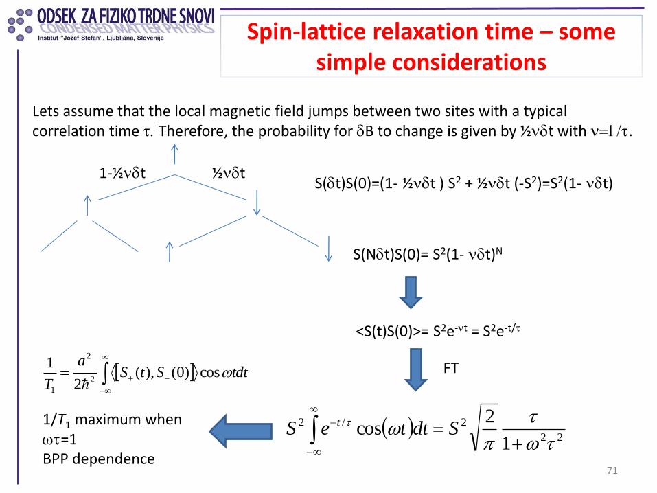
Spin-lattice relaxation time – some simple considerations

71

Lets assume that the local magnetic field jumps between two sites with a typical correlation time t. Therefore, the probability for B to change is given by ½t with =1/t.

S(t)S(0)=(1- ½t ) S2 + ½t (-S2)=S2(1- t) ½t 1-½t

S(Nt)S(0)= S2(1- t)N

<S(t)S(0)>= S2e-t = S2e-t/t

FT

22

2/2

1

2cos

t

t

pt

=

SdtteS t1/T1 maximum when t=1 BPP dependence

= tdtStSa

Tcos)0(),(

2

12

2

1


72

Lets now assume, that the fluctuation field comes from the electronic field through the hyperfine coupling intercation Expressing B we finally get for T1

After Fourier transformation Finally we fluctuation-dissipation theorem, which states To get T1 in the high-T expansion

== BItSaIH nii

g)('

= tdtStSa

Tcos)0(),(

2

12

2

1

=i

rq

iqieSS

[A,B]=(AB+BA)/2

=q

qqqq tdtStSAAT

cos)0(),(2

11

1

kT

e

qqe

qtdtStS

/21

),(''2cos)0(),(

2

1g

=

=q

qq

e

n qAA

kT

T

g

g ),(''212

2

1

Spin-lattice relaxation in metals

73

rSIgH Bhf

32

3

8gm

p=

The perturbing interaction is the s-contact interaction Transitions from state |k m> to |k m+1> where m is the initial nuclear quantum number

kkhfmkmkEEmkHmkP =

'

2

1'1'

2

p

)1)(()0()0(3

41'

2

'

22

= mImIuumkHmk kkenhf gg

p

We take Bloch WFs and calculate the corresponding matrix elements We make an approximation that all states in the vicinity of Fermi surface have approximately the same probability density at the nucleus. Next we need to sum over all k and k’ states then we can finaly write

=

',

'

222

1

)0(3

441

kk

kkken EEuT

ggpp

Spin-lattice relaxation in metals

74

It is important to bear in mind, that the sum over k,k’ is restricted to states fully occupied at k and empty at k’. The sum over k can be replaced by the integration over energy with introducing the density of states n(E), i.e. n(E) dE. The occupation restriction is eforced with the Fermi occupation function f(E)=[exp((E-EF)/kT)+1]-1. The summation then becomes

2

222

1

)()0(3

441Fken

B EnuTk

T

=

gg

pp

'))'(1)(()'()(' EEEfEfEnEndEdE

FBB EETkE

fTkEfEf =

= ))'(1)((

Remember Knight shift:

p 2

03

8

FEkuK =

22

1

41

e

Bk

TKT g

p

=

Famous Korringa relation The final result depends only on elementary constants and not on materials; this hold only for simple metals, where correlations can be neglected

Korringa relation - examples

75

22

1

41

e

Bk

TKT g

p

=

In practice, simple Korringa relation is not satisfied. Let’s check some simple alkali metals

metal KS(%) T1T (exp) T1T (calc) ratio

7Li 0.0263 45 Ks 26 Ks 0.58

23Na 0.112 4.8 Ks 3.1 Ks 0.65

63Cu 0.232 0.7 Ks 0.7 Ks 0.78

Various corrections can be made to Korringa relation. In principle electron-electron interaction potential can enhance the spin susceptibility thus correcting K.R. in the right way. However, exchange fluctutations would also enhance spin-lattice relaxation. We will come to this point latter, but for now we just introduce Korringa factor , which should be <1 (AFM) fluctutaions, >1 (FM) fluctuations

g

p22

1

41

e

Bk

TKT =

13C NMR in K3C60

Yoshinari et al. (1993)

Korringa relation - corrections

76

Various corrections can be made to Korringa relation. In principle electron-electron interaction potential can enhance the spin susceptibility thus correcting K.R. in the right way. However, exchange fluctutations would also enhance spin-lattice relaxation. We will come to this point latter, but for now we just introduce Korringa factor , which should be <1 (AFM) fluctutaions, >1 (FM) fluctuations

g

p22

1

41

e

Bk

TKT =

Stoner enhancement factor

0

0

1

=

=<(1-q)2/(1-0)2>EF

Spin-lattice relaxation time – some simple considerations

77

To a reasonable appoximation we may try to write Then Where ex=[2zkB

2J2S(S+1)/3ħ2]1/2

e

n

ne

ne qqq

)0,()0,(),(''

22

=

=

q e

qq

e

n qAA

kT

T

g

g )0,(212

2

1

C

Example: YBa2Cu3O7-y

Moriya expression

=

j

jj

n

n

iCA

ATT

)exp()(

),()(

1 2

1

rqq

qq

q

CuO2 layer with Cu2+ localized moments

63Cu

17O

Mila & Rice, Physica C 157, 561 (1990)

B

A

2

222

17

2263

17

63

cos4)(

coscos2)(

2

)4(

aq

yx

s

s

xCA

aqaqBAA

CK

BAK

=

=

=

=

q

q

A: on-site coupling B,C: transferred couplings

Millis, Monien & Pines PRB 42, 167 (1990)

a Millis, Monien and Pines assumed that the spin dynamics is described by

G=

2

22

4

0

0 11),(lim

p

AFMqq

q

0)(

4)(

,

217

2263

=

=

=

AFM

AFM

aaAFM

A

BAA

q

q

q pp

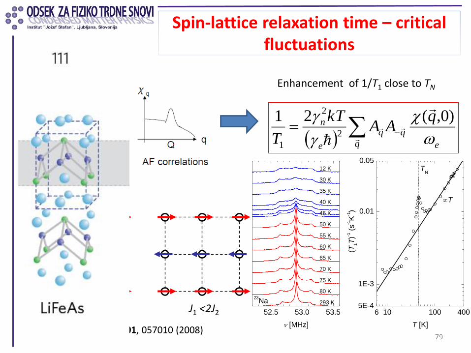
Spin-lattice relaxation time – critical fluctuations

79

Enhancement of 1/T1 close to TN

Yildirim, PRL 101, 057010 (2008)

Checkerboard AFM

J1 J2

J1 >2J2 J1 <2J2 6 10 100 4005E-4

1E-3

0.01

0.05

52.5 53.0 53.5

293 K

80 K

75 K

70 K

65 K

60 K

55 K

50 K

45 K

40 K

35 K

30 K

12 K

23Na

T

TN

(T1T

)-1 (

s-1K

-1)

T [K]

[MHz]

=

q e

qq

e

n qAA

kT

T

g

g )0,(212

2

1

Example: LiFeAs

Localized Fe2+ spins Itinerant Fe 3d electrons

57Fe

75As

C

B

A

2

2

2

222

75

75

coscos16)(

4

aqaq

s

yxCA

CK

=

=

q

a

22

75

75

)( cA

cK s

=

=

q

For noninteracting spins can be taken out of the summation. In this limit we can calculate 0 and 0’ for the localized spins and itinerant scenario. If

n

nATT

),()(

1 2

1

qq

q

),( n q

= Cc 44

coscosdd16C

dd16C

)(

2

2

2

22

2

2

2

0

0

==

==

aqaq

yx

yx

yxqq

qq

A

c

q

q

q

Supported by density-functional calculations: - Katrin Koch & Helge Rosner, MPI-CPfS - Calculated electric-field gradients correctly reproduce the experimental values for both 75As and 7Li sites.

Jeglič et al., ArXiv: 0912.0692

A B

Example: AFM fluctuations in LiFeAs

How strong are AFM fluctuations in LiFeAs? 1. We cannot unambiguously discriminate between the on-site Fermi contact (itinerant) and the transferred coupling mechanism (localized moment at the Fe sites). 2. Cross-terms between different bands in the LiFeAs multiband structure can modify Korringa relation.

Korringa factor , measured for LiFeAs (green circles) and SrFe2As2 (red circles). Horizontal dashed lines indicate expected values for noninteracting electrons. If the transferred coupling is active, 1/T1T is enhanced for a factor of 15±5!

0 100 200 3000.0

0.2

0.4

0.6

0 100 200 3000

1

2

3

4

0.0

0.1

0.2

0.3

T (K)

1/(

T1T

) (s

-1K

-1)

T (K)

0'

0

(c)

(b)

(a)

LiFeAs

SrFe2As

2

Ks (

%)

Jeglič et al., ArXiv: 0912.0692

Summary

NMR = local, real-space probe where the behaviour of nuclear spins can be monitored on a site-to-site basis. Observables: - NMR spectrum - Relaxation rates

Hyperfine interaction (Fermi contact, transferred hf, dipolar interaction) Knight shift, shift in the superconducting state Spin-lattice relaxation rate, Korringa relation

=q

qq

e

n qAA

kT

T

g

g ),(''212

2

1

Acknowledgements

83

Ljubljana: Peter Jeglič, Martin Klanjšek, Andrej Zorko, Anton Potočnik, Kristjan Anderle

and Andraž Kranjc

www.lemsuper.eu

Documents

Nuclear magnetic resonance in magnetic systems and metals