Embed Size (px)
Citation preview

Nuclear Magnetic Resonance:
a quantum technology for computation and
spectroscopy
H. K. Cummins∗
Oxford Centre for Quantum ComputationClarendon Laboratory
Parks RoadOxford OX1 3PU
J. A. JonesOxford Centre for Quantum Computationand Oxford Centre for Molecular Sciences
New Chemistry LaboratorySouth Parks RoadOxford OX1 3QT
August 3, 2000
AbstractIn this article we consider nuclear magnetic resonance (NMR) as
an example of a quantum technology; we consider in particular de-tail the implementation of quantum computers using NMR. We beginby outlining the physical principles underlying NMR, and give an in-troduction to the quantum mechanics involved. We next discuss thegeneral characteristics of quantum technologies and the ways and ex-tent to which these characteristics are expressed in NMR. We thengive an introduction to the subject of quantum computation and itsimplementation using NMR. Finally, we describe some spectroscopytechniques which also exploit the quantum nature of NMR.
∗To whom correspondence may be addressed.
1

1 Introduction
Quantum physicists become accustomed to the glamour of their field. Theirsubject is the very small, the very strange, the theoretically forbidden, and,usually, the very difficult. It is easy to forget, after wrestling with the moreexotic aspects of the microscopic world all day, that quantum physics mightalso include aspects which are concrete, wet, and, worst of all, occasionallyorganic. One of these disconcertingly substantial facets of quantum mechan-ics is Nuclear Magnetic Resonance spectroscopy (NMR). While physicistsgenerally leave NMR to chemists, biochemists, and doctors, NMR does infact have many interesting quantum aspects; liquid-state NMR is an unusualand often overlooked example of a quantum technology. NMR has recentlybeen used to perform quantum computations which use quantum effects toachieve non-classical increases in computational efficiency. Many spectro-scopic techniques also exploit quantumness to extract otherwise inaccessiblegeometric information about a molecule or to probe uncooperative atomsby giving them the attributes of more cooperative atoms.
2 Basics of NMR spectroscopy
Nuclear magnetic resonance was first observed in 1946 by two groups whoindependently probed the behaviour of the hydrogen nuclei (in water andparaffin) in strong magnetic fields. The physicists who discovered it antici-pated it would be an ideal method for measuring the magnetic moments ofvarious atomic nuclei, but further investigation revealed that the resonancefrequency of a nucleus was influenced by its chemical environment. Thisunfortunate dependence on chemical details made the technique useless forthe simple physical experiments envisioned but simultaneously transformedit into a valuable spectroscopic tool [1]. NMR is now an important analyticmethod in many fields, including chemistry, biology, medicine, materialsscience, and geology.
In essence, NMR is the study of transitions between the Zeeman levelsof an atomic nucleus in a magnetic field. For experimental and theoreticalconvenience, attention is often restricted to the spin-half nuclei. In thepresence of a magnetic field Bz, directed along the z-axis, the degeneracy ofthe two spin states of a spin-half nucleus is lifted by the Zeeman Hamiltonian,
H = −12~γσzBz (1)
where γ (the gyromagnetic ratio) is a constant characteristic of the nucleus
2

and σz is one of the Pauli spin matrices. The allowed energy levels aremultiples of the eigenvalues of σz; that is,
E = ±12~γBz (2)
In order to make E a reasonable size, Bz is made as large as possible by usingsophisticated superconducting electromagnets. The most advanced of thesehave fields around 20 T, which is approximately 400 000 times the earth’smagnetic field, while typical laboratories might have magnets whose fieldis about 5–15 T. These extraordinarily strong magnets are also elaboratelyengineered to set up fields which are homogeneous across the sample towithin one part in 1010.
What justifies this level of effort in manufacturing strong homogeneousmagnets and makes equation (2) interesting is that the precise Bz expe-rienced by a nucleus in a magnetic field, while largely determined by themagnet, is also affected by tiny fields set up by any nearby electrons, sothat the same nucleus in different chemical environments will have slightlydifferent energy levels. The presence of such a set of energy levels can bedetected by spectral absorption as long as we can control some interactionthat causes transitions between levels; in the case of NMR this is providedby the coupling between the nucleus and a rotating (or alternating) mag-netic field applied perpendicular to the main field with an angular frequencysuch that
~ω = ∆E (3)
where ∆E is the spacing between energy levels, and ω lies in the radiofre-quency region of the spectrum for currently achievable magnetic fields.
Although what we have described is already a useful tool for chemicalanalysis, it doesn’t incorporate any of the spookier features of quantum me-chanics. To do this, we need to turn our attention to molecules which containmore than one spin-half nucleus, since the second important interaction inliquid-state NMR, responsible for the creation of non-classical correlationsbetween spins, arises from spin–spin interactions in these systems. Perhapssurprisingly, the most important spin–spin coupling is not dipole–dipole cou-pling: the nuclei do interact with one another as dipoles, but these magneticinteractions are averaged out in liquids by rapid molecular tumbling. Thereis a second interaction between nuclei, related to the Fermi contact inter-action and mediated by shared valence electrons, which is not averaged outcompletely. This coupling is known as the scalar or J-coupling. It is directly
3

observable in NMR spectra as a splitting in the NMR signals correspondingto each nucleus, as shown in figure 1.
Figure 1: Cytosine and its NMR spectrum when dissolved in deuteratedwater (D2O). The two sets of peaks each correspond to a signal from ahydrogen atom. For chemical reasons, only the two hydrogen atoms (thewhite spheres) bonded to carbon (black spheres) give rise to NMR signals.The other three undergo rapid exchange with deuterium in the solvent (lightgrey spheres).
A substantial scalar coupling is only seen between two nuclei if theyshare significant electron density, implying they are close together in thesame molecule. Close means logically close, not spatially close: the twonuclei must be connected by a small number of chemical bonds. When thecoupling between two nuclei is small compared with the difference betweentheir NMR frequencies (weak coupling) the coupling Hamiltonian takes thesimple form
H = J12 (σz1 ⊗ σz2) (4)
where J12, the spin–spin coupling constant, depends on the details of themolecular structure, but is typically in the range 1 Hz to 1 kHz.
Note that the J-coupling Hamiltonian is not applied to the system fromoutside. Instead, it is an inherent interaction which will be manifested anytime the system is allowed to evolve naturally (‘free precession’). Taking intoaccount the Zeeman effect and the spin–spin coupling, the total Hamiltonianof a two spin system is
H = 12
(ω1 (σz1 ⊗ I2) + ω2 (I1 ⊗ σz2) + 1
2J12 (σz1 ⊗ σz2))
(5)
The notation σz1 simply means ‘an ordinary σz matrix that is here beingused in reference to the first spin’, and I2 similarly means ‘an ordinary
4

identity matrix that pertains to the second spin’. The identity matricesare necessary so that the matrix sums make sense. For a system with nspins, the Hamiltonian will have n Zeeman terms and 1
2n(n − 1) couplingterms, although some coupling terms may be so small that they can be safelyneglected.
2.1 Representations of quantum states
Having determined the Hamiltonian and the allowed energy levels of thesystem, we now turn to its allowed states. The simplest possible quantummechanical system consists of one particle whose state is described by thestate vector |ψ〉. Because of quantisation, the particle will have a fixednumber of discrete energy levels; we are considering a spin-half system, sowe restrict it to two levels which we call |0〉 and |1〉. The spin is a quantumobject and can therefore exist in a superposition of these levels: a generaldescription of its state is |ψ〉 = α |0〉+β |1〉, where α and β are both complexnumbers and αα∗ + ββ∗ = 1. Written another way,
|ψ〉 =[
αβ
](6)
The density matrix representation of this same state is
ρ = |ψ〉 〈ψ| =[
αα∗ αβ∗
βα∗ ββ∗
](7)
For example, the state (|0〉+ |1〉) /√
2 can be represented as
|ψ〉 =1√2
[11
]or ρ = |ψ〉 〈ψ| = 1
2
[1 11 1
](8)
We can always express ρ in the form ρ = 12 (I+ sxσx + syσy + szσz), a
linear combination of the Pauli spin matrices, subject to the constraints thatsx, sy, and sz are all real and s2
x + s2y + s2
z = 1. Once we have written it inthis form, it is natural to picture ρ as a unit vector called the Bloch vector.Figure 2 shows the Bloch representation of (|0〉+ |1〉) /
√2.
What about multiple particles? One obvious way of representing largersystems is to use tensor products of representations of smaller systems: ρ =σ1 ⊗ σ2 ⊗ · · · ⊗ σn. For example, a system with two particles, one in an
5

+z
-z
+x-y
+y-x
Figure 2: Bloch vector representation of the state (|0〉+ |1〉) /√
2.
equally weighted superposition and one in the state |0〉, is represented by
ρ =12
[1 11 1
]⊗
[1 00 0
]=
12
1 0 1 00 0 0 01 0 1 00 0 0 0
(9)
However, quantum mechanics also allows many multi-particle quantum stateswhich cannot be decomposed into products of constituent states and there-fore cannot be represented in this way. These states are known as inseparableor entangled. For example, consider the two particle state
ρ =12
(|01〉+ |10〉) (〈01|+ 〈10|) =12
0 0 0 00 1 1 00 1 1 00 0 0 0
(10)
for which no decomposition into single particle subsystems exists. (Thereader can easily verify this by trying to factor the density matrix.) Thisrepresentational difficulty hints at an underlying physical difficulty. Insepa-rability implies that the information about the state of any particular par-ticle in an inseparable system is not ‘owned’ by the particle, but is rathershared between two or more particles in the system. Einstein, Podolsky,and Rosen suggested that this implied the particles were ‘communicating’
6

with one another faster than light, a violation of special relativity [2]. Theyargued this apparent paradox could be only be resolved by the introductionof hidden variables to restore determinism and locality behind the scenes.In 1964 Bell proved that that a theory with local hidden variables couldbe experimentally distinguished from one without them and subsequent ex-periments seem to have ruled out the possibility of local hidden variables[3, 4].
The importance of entanglement to quantum mechanics cannot be un-derestimated. Schrodinger said ‘he would not call that one but rather thecharacteristic trait of quantum mechanics, the one that enforces its entiredeparture from classical lines of thought’ (cited in [5]). Entanglement andthe associated paradoxes of non-locality have been dealt with extensively inthe literature, but see references [6, 7, 8] for an introductory discussion.
Is there a way of visualising multiparticle states that is analogous tothe Bloch representation for a single state? The answer is, unfortunately,no. Separable states can be represented as a set of Bloch spheres, but theBloch representation breaks down for more general states and no satisfactoryalternative is known. Although this is inconvenient, it should not comeas too great a surprise: the correlations between entangled states are sofundamentally removed from our everday understanding of nature that itwould be surprising if there were a means of representing them with a pictureor simple classical analogy.
A second representational issue arises when we try to represent partsof larger systems. Say we would like to represent, however inadequately,the state of the first particle in the system described by equation (10). Wecan do this by averaging (‘tracing’) over the possible states of the secondparticle, which gives us
ρ =12
[1 00 1
](11)
Since equation (10) describes an inseparable state, we know this representa-tion is to some extent wanting, and we would like a way of quantifying thefact that important information is missing. Notice that, while ρ is ordinarilydefined to be |ψ〉 〈ψ|, there is no way of writing equation (11) as a product ofstate vectors. This is a general property of fragments of entangled systemsand we call density matrices of this type mixed. The state described by (10)is in fact the maximally mixed state. Formally, a density matrix is mixed if
7
it cannot be written in the form
ρ = |φi〉 〈φi| (12)
but must instead be represented as a sum of several such outer products.For example, the matrix in (11) can be represented as as 1
2 |0〉 〈0|+ 12 |1〉 〈1|.
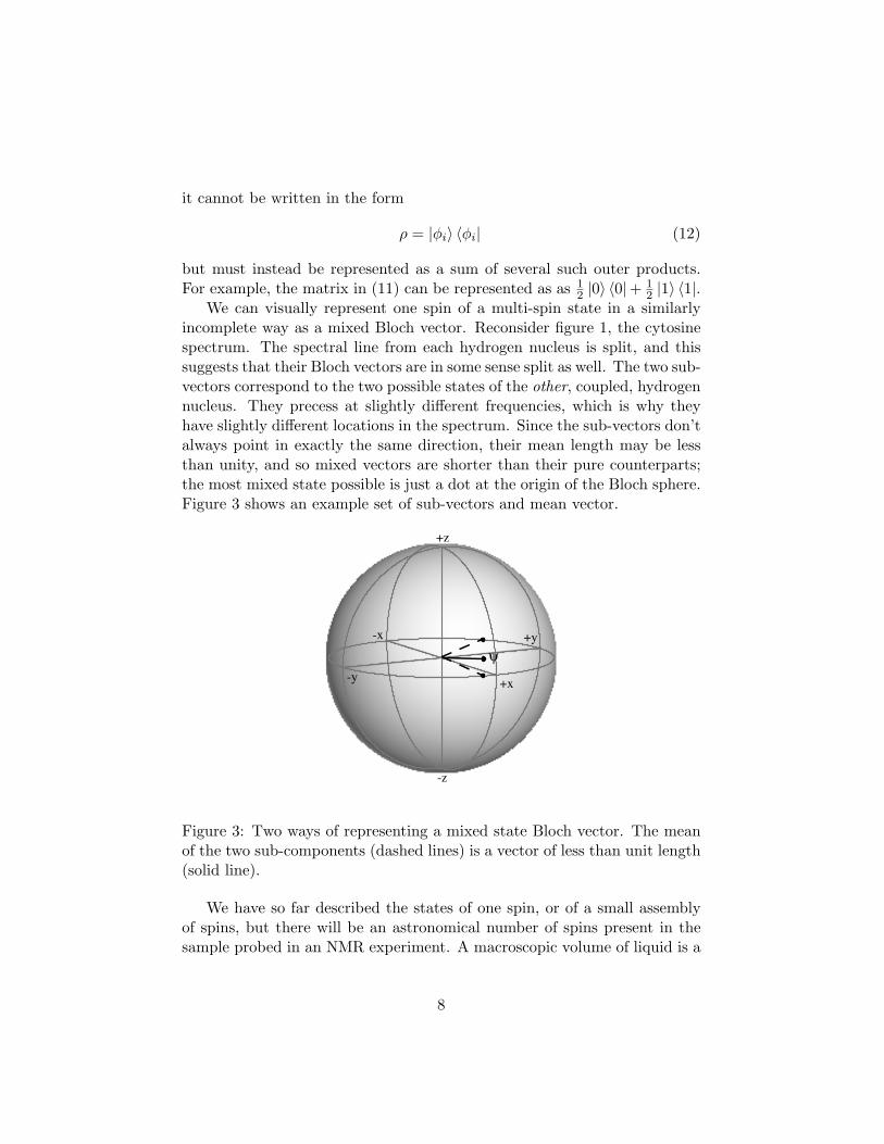
We can visually represent one spin of a multi-spin state in a similarlyincomplete way as a mixed Bloch vector. Reconsider figure 1, the cytosinespectrum. The spectral line from each hydrogen nucleus is split, and thissuggests that their Bloch vectors are in some sense split as well. The two sub-vectors correspond to the two possible states of the other, coupled, hydrogennucleus. They precess at slightly different frequencies, which is why theyhave slightly different locations in the spectrum. Since the sub-vectors don’talways point in exactly the same direction, their mean length may be lessthan unity, and so mixed vectors are shorter than their pure counterparts;the most mixed state possible is just a dot at the origin of the Bloch sphere.Figure 3 shows an example set of sub-vectors and mean vector.
ψ
+z
-z
+x-y
+y-x
Figure 3: Two ways of representing a mixed state Bloch vector. The meanof the two sub-components (dashed lines) is a vector of less than unit length(solid line).
We have so far described the states of one spin, or of a small assemblyof spins, but there will be an astronomical number of spins present in thesample probed in an NMR experiment. A macroscopic volume of liquid is a
8

complicated and superficially unquantum object, and we would prefer to ig-nore the bulk of the liquid and investigate a single molecule whose quantumbehaviour we can analyse mathematically. Could we do this by using spa-tial localisation techniques, like those used in magnetic resonance imaging,to pick out individual molecules? Although this technique would be con-ceptually tidy, it is not practical for several reasons. The signal from anyindividual molecule is extremely weak, around 2µeV, so making measure-ments with reasonable signal to noise would be extremely difficult, althoughperhaps not absolutely impossible. More seriously, molecules are tiny, andeven the spacing between them is very small, so achieving sufficient spatialresolution would be tricky. Even were the spatial resolution fine enough,however, the rapid motion of molecules in solution means that the targetedmolecule would soon diffuse out of the selected region.
We are therefore forced to detect the combined signal from all the molecules.Fortuitously, however, we can almost entirely neglect the macroscopic na-ture of the observed system. The mathematical representation of the ap-parent state of an NMR system is considerably simpler than the represen-tation of its actual state. Taking the number of spins in the system to beP , the full density matrix of the system has 2P elements, making detailedquantum mechanical calculations hopeless. However, rotational averagingreduces dipole–dipole coupling between spins in neighbouring molecules toa second-order effect, and so the system can be considered in terms of aneasily-manipulated reduced density matrix of size 2n, where n is the numberof spins in any one molecule. Instead of being one monstrously complicatedsystem, the molecules in solution behave like an ensemble of small discretesystems. They are isolated from one another by dipole averaging, and fromthe external environment by simple surface to volume considerations of theliquid. Nonetheless, the macroscopic and ensemble aspects of the systemare not entirely without implications; we will discuss some of the more in-teresting ones later.
2.2 Representations of quantum operators
Like quantum states, quantum operations are conveniently represented asmatrices, given by
U = exp(∫ τ
0−iH dt
)(13)
where U is the propagator, H is the operation’s Hamiltonian, and ~ is setto unity. Although in principle each operation has a unique matrix repre-
9

sentation, global phase factors are meaningless in NMR. The propagatorsof Hamiltonians which differ only by a multiple of the identity matrix differonly by a global phase factor, and so these Hamiltonians are in practice ex-perimentally indistinguishable. All propagators obey one constraint, whichis that they must be unitary. This is an expression of the quantum mechan-ical axiom that all quantum operations are reversible.
Any unitary operation on a spin can be described a rotation about someaxis. In the case of RF pulses, this correspondence is particularly naturalbecause a given rotation angle corresponds in practice to a pulse duration,θ = τω, the angle of the axis in the xy-plane corresponds to the phaseof the RF field, and the declination of the axis from the xy-plane (if any)is determined by the field’s detuning. For example, we would write theoperator given by application of the Hamiltonian H = ωσx for a period ofτ = π/ω as
U = exp
(∫ πω
0−1
2 iωσx dt
)=
[0 −i−i 0
]= 180x (14)
Operators that arise from the J-coupling affect the relations between spinsand so they cannot be conveniently described as rotations; instead, they aresimply described in terms of time periods. The operator for the J-couplinghas the general form
U =
exp(−1
4 iJt)
0 0 00 exp
(14 iJt
)0 0
0 0 exp(
14 iJt
)0
0 0 0 exp(−1
4 iJt)
(15)
for a coupling of strength J over a time t. Since we generally want Jt to besome dimensionless fraction, we describe the operator as a time in units of1/J , for example, π/(4J).
3 Basics of quantum technologies
Quantum effects are manifested in a wide array of physical systems, butnot every system in which quantumness is observable ought to be consid-ered an example of a quantum technology. Technologies are sets of tools,techniques, and concepts which together provide a means of manipulating asystem into performing a task. This task cannot simply be the elucidationof the techniques and concepts involved—while a pencil can be described as
10

a simple technology for writing, it cannot be sensibly described as a tech-nology for learning about pencils, or, worse yet, as a technology for being apencil. Similarly, a quantum technology must achieve some goal beyond themanipulation and observation of the system’s own quantum nature. Despitethis qualification, manipulation and observation of quantumness are impor-tant technical pre-requisistes of any quantum technology. For the class oftechnologies we are considering, those which relate to quantum informationprocessing, two kinds of manipulation are required: the ability to control theevolution of the system (Hamiltonian sculpting), and the ability to controlthe starting state of the system (initialization). Observation is a necessaryfinal step, so that we can read out the answer of our computation or thetransmitted information. Both readout and initialization are complicatedby the ensemble nature of NMR in ways that are often unfortunate but alsounexpectedly interesting.
3.1 Ensemble quantum technologies
It is surprising that a system so tangibly macroscopic as liquid in a testtube should be a viable quantum technology. The bulk nature of NMRdoes in fact have several repercussions at the quantum level, some of whichare more fundamental than others. These implications have experimentalinterest in themselves, and they also force us to think deeply about some ofthe finer points of quantum mechanics. The study of the ensemble aspects ofNMR is controversial and has inspired a number of theoretical investigationsinto previously unexplored aspects of quantum mechanics. For a generaldiscussion of the issues involved, see reference [9].
We instinctively associate quantum mechanical behaviour with the verysmall. Quantum mechanics was not developed until technology advanced tothe point where scientists were able to investigate the tiniest constituentsof matter directly. The very small, it seemed, had a variety of bafflingand essentially disturbing behaviours that weren’t manifested by the largerobjects that had previously been used as the benchmark of normality. How-ever, once scientists had adjusted to quantum jumps, superpositions, andapparent action at a distance, they stopped asking why small things didn’tact like big things, and started wondering why big things didn’t act likesmall things. The general conclusion was that macroscopic systems deco-here rapidly, and that this dilution of the quantumness is responsible for theapparently ‘normal’ behaviour.
Decoherence is an important concept in the quantum mechanics of themacroscopic. A system becomes decohered if it interacts with its environ-
11

ment, since this interaction causes information about the system to be spreadthrough the environment; when the environment is traced out this informa-tion is lost. Having decohered corresponds to being in a mixed state; acompletely decohered system is in the maximally mixed state—that is, thedensity matrix is a multiple of the identity matrix.
When we consider a test tube of liquid in a spectrometer, we mentallydivide the state of each molecule into two parts: a large undetectable max-imally mixed portion, and a small detectable (‘effective’) portion, ρ0:
ρ = (1− ε)I/N + ερ0. (16)
where N = 2n and n is the number of qubits in the molecule. Coherentstates can be temporarily excited only in the ρ0 part. These excited stateswill themselves decohere (‘relax’) by interacting with one another and theenvironment. There are a number of factors that determine how long thisrelaxation takes, including the previously neglected dipole–dipole interac-tion. Luckily, however, decoherence of the effective state is not a criticalconsideration in NMR since the relaxation times are long enough that wecan conduct complex experiments without crippling losses to decoherence.The mental division into effective state and undetectable maximally mixedstate allows us to largely neglect the ensemble nature of NMR; nonetheless,the presence of many copies of ρ0 does present problems, particularly in theinitialization and readout of quantum states.
3.2 Observation
Even the small, undecohered, part of an NMR experiment contains multi-ple copies of the effective state, and this ensemble nature has an immediatepractical implication. It is an axiom of quantum mechanics that a measure-ment of a state |ψ〉 = α |0〉 + β |1〉 will return, at random, either 0 withprobability |α|2 or 1 with probability |β|2 (assuming the measurement wasmade in the computational basis). The measurement will project |ψ〉 intoone of |0〉 or |1〉; if we got an answer of 0, |ψ〉 = |0〉 after the measurement;if the measurement gave 1, |ψ〉 will be turned into |ψ〉 = |1〉. The measure-ment returns only partial information about the true state and collapses itin the process. In an NMR measurement, on the other hand, a measurementof an effective state |ψ〉 is in fact a measurement of a whole set of |ψ〉s; itcan only return mean values of α and β, and the superposition will not bedestroyed by the measurement. Being able to measure the average popula-
12

tion non-destructively seems like a wonderful advantage, but many quantuminformation processing techniques rely on projective measurement.
These difficulties aside, the mechanism of observation in an NMR systemis very simple. Spins in a superposition will precess around the z-axis,while spins with no component in the xy-plane are in an eigenstate andwill not precess. Ensembles of precessing spins give rise to a precessing netmagnetic moment which, by Faraday’s law, induces a voltage in a receivercoil. We can measure the magnitude and phase of the detected signal anddraw conclusions about the declination of the net magnetic moment fromthe z-axis and its phase. The magnitude of the observed signal will decreaseas the system relaxes to equilibrium, and so this measurement process iscalled ‘free-induction decay’. It is usually necessary to apply a 90◦ pulseto the system before measurement, since this has the effect of knockingz-magnetisation (an eigenstate) down into the xy-plane where it can beobserved.
3.3 Hamiltonian sculpting
The power and utility of NMR as a quantum technology stems from themalleability of the NMR Hamiltonian. Terms can be modified or suppressedentirely, almost at will. This allows the experimenter precise control over theinteractions within the system and the response of the system to externalprobing. The terms in the NMR Hamiltonian, given in equation (5), areinherent to the system and cannot be changed, but the average Hamiltonianover some period depends on the inherent Hamiltonian equation (5) and alsowhatever RF field Hamiltonians may have been applied. Its form may beconsiderably simpler than that of the inherent Hamiltonian. The literaturedealing with the various possible manipulations of the average Hamiltonianis vast, but we will briefly describe some of the more important techniques.
The most basic and useful manipulation is the spin echo. Spin echoescan, among other things, undo the effects of spatial inhomegenities in themagnetic or RF field, suppress specific interactions, and refocus the effectsof chemical shifts. Spin echoes can be understood by analogy with a budgettape-deck whose fast-forward and rewind buttons have both broken. Inorder to return the tape to its initial position after playing it for some timeτ , it is necessary to take the tape out, flip it over, and then play it again fora time τ . The important idea is that the action of time can be in some sensebe reversed by flipping the system. The spin echo is also analogous to acolony of lemurs who leave their nest in a group to go forage in the morning.Some leap quickly through the trees, while others scurry more slowly on the
13

!
lemur nest
!
alarmed lemurs
hungry fossa
Figure 4: When lemurs spot a fossa in the distance, they return to theirnest. Lemurs in the trees are further from the nest but are able to jumprapidly from branch to branch, returning home at the exact same time asthe lemurs on the ground.
ground, so the lemurs are soon dispersed through the forest. When one ofthe lemurs spots a predatory fossa in the distance and raises an alarm, allthe lemurs turn around in dismay and head back to the nest. The lemursin the trees make rapid progress, but they’re further out from the nest thanthe slow-moving ones on the ground, and so the lemurs necessarily all arriveback at the nest in a clump at the same time. This process is illustrated infigure 4. Viewed thermodynamically, this restoration of the dispersed anddisordered lemur population into a neat group might seem like an unphysicalviolation of the second law of thermodynamics, but this is not the case; theunitarity of the dispersal process means that there is no increase in entropyassociated with it, and there is therefore no decrease in entropy associatedwith its reversal. While they are most commonly used in NMR, spin echoesare by no means unique to NMR, and they may find wide application infuture quantum technologies.
The normal course of events in an NMR experiment is that an RF pulse
14

is applied to the sample to excite it, signal appears, and then the signalgradually disappears as the sample decoheres back to thermal equilibrium. Itis certainly not normal for signal to appear when no pulse has been applied,but this is exactly what happens in a spin echo experiment; a 180◦ pulseis applied after the signal has disappeared, nothing happens for some time,and then signal spontaneously reappears. This resurrection of a decayedsignal was initially quite startling, not least to the discoverer of the spinecho, Erwin Hahn. The reason the spin echo works is that much of whatappears to be decoherence in NMR is in fact dephasing across the sample.Dephasing is unitary and can therefore be reversed with an appropriate pulsesequence.
Consider the two-spin Hamiltonian, (5), again. In addition to reversingdephasing error terms, spin echoes can be used to suppress any two of itsthree terms, or, in longer combinations, any one of its terms. Selectively ap-plying a 180◦ pulse to the first spin undoes its evolution and the effects of theJ-coupling but allows the second spin to evolve, selectively refocussing thesecond spin similarly kills the ω2σz2 term and the J12 (σz1 ⊗ σz2) term butkeeps the ω1σz1 term, while simultaneously refocussing both spins deletesthe ω1σz1 and ω2σz2 terms but keeps the J-coupling term. Refocussing thefirst and second spins at different times removes the J-coupling term butmerely scales down both evolution terms. For systems with more spins, thepulse sequences for creating arbitrary scaled down Hamiltonians are longerbut not unreasonably so.
A second, less versatile, sculpting technique is spin decoupling. J-couplingsto a specific nucleus can be eliminated by continuously applying a field atthe resonant frequency of the offending nucleus. This causes rapid transi-tions between its |0〉 and |1〉 states, which causes rapid flips between thesub-vectors of the coupled nuclei. If these flips are sufficiently rapid, it willbe impossible to distinguish the two components of the Bloch vector and nosplitting will be observed in the spectrum. As a side-effect, all signal fromthe target nucleus is obliterated, which is sometimes undesirable.
3.4 Controlling the starting state
Hamiltonian sculpting allows us to precisely control the evolution of an ef-fective quantum state, and so it seems that driving a system into an effectivestate of our choosing ought to be a trivial problem. Unfortunately, the op-erations we can achieve by Hamiltonian sculpting are all reversible, and thisseverly limits the states we can achieve. As initialization requires that thesystem be placed in some state |ψ〉, independent of its state before the be-
15
ginning of the initialization process, it manifestly cannot be achieved by anyreversible process. Initialization schemes must therefore be quite differentfrom ordinary operations.
In many quantum technologies, initialization is achieved by cooling tothe ground state. This is not a practical approach for NMR, as the energygaps involved are tiny compared with the Boltzmann factor at any reason-able temperature. Instead, three alternate experimentally accessible pro-cesses with non-unitary effects are commonly exploited in NMR. These arerelaxation, magnetic field gradients, and phase cycling. The first of theseis the simplest, since it requires no special equipment or post-processing,and is, in fact, inevitable. Relaxation brings the system into a reproduciblethermal equilibrium which is an adequate starting state for many purposes.The second technique, gradient crushing, relies on the fact that the sam-ple forms a macroscopic ensemble; by applying Hamiltonians which varyover the sample the ensemble averaged evolution can be non-unitary. Thisis most commonly achieved by momentarily destroying the spatial homo-geneity of the main magnetic field, but similar effects can be achieved usingspatially inhomogeneous RF fields. The last approach relies on combiningthe results of several subtly different NMR experiments by post-processing;as this is done by classical methods, such processing is not confined to uni-tary transformations. In conventional NMR experiments this is referred toas phase cycling, and plays a central role in many sequences, although formany purposes it has now been replaced by the use of gradient techniques.In practice spectroscopic techniques normally rely on relaxation to initializethe system, while quantum computation usually requires the more sophisti-cated gradient crushes or phase cycling.
Because initialization by relaxation is so effortless, it is easy to under-estimate its importance as an initialization technique. The reproducibilityof NMR spectroscopy relies on the well-defined nature of the relaxed state.More critically, relaxation into thermal equilibrium is necessary before a netmagnetic moment arises. The earliest attempts at an NMR experiment, byDutch physicist C. J. Gorter, famously failed because he happened to choosea sample with an unusally long relaxation time, which meant the system didnot achieve its initialized state before measurements were attempted.
While all of the initialization processes described allow for the manipu-lation of the effective state, none, even the most non-unitary, allows for themanipulation or elimination of the maximally mixed portion of the NMRstate. The silent presence of this large decohered volume of solution presentssome fundamental issues. A widely used criterion for quantumness (in thesense of ‘provable non-classicalness’) is separability. A non-separable state
16

clearly has some entanglement (the converse assertion is mathematicallyirrefutable but nonetheless more philosophically controversial). By defini-tion, the effective state of an NMR system exhibiting entanglement is non-separable, but the state of the entire volume of solution has been shown tobe separable for low polarisation, implying a ‘classical’ description of thestate exists [10]. It has not been shown, however, that transformations be-tween these ‘classical’ states can be described classically [11]. This forcesa reconsideration of the notion that entanglement is the defining featureof quantum mechanics, since non-entangled systems can apparently displaynon-classical behaviour. NMR has made it clear that entanglement is as yetpoorly understood within the quantum mechanics community, and mixedstate entanglement is currently a very active research area [10, 11, 12].
4 Quantum computation
Hamiltonian sculpting gives us the tools needed to manipulate quantumspins and the relationships between them. Currently, the most intriguinguse of this power is as a means of implementing quantum computers. Quan-tum computers are information processing devices which operate by andexploit the laws of quantum mechanics, potentially allowing them to solveproblems which are intractable using classical computers [13]. They canimplement new types of quantum mechanical algorithms which are far morecomputationally efficient than their classical equivalents. The first of thesequantum algorithms to be described was Deutsch’s algorithm [14, 15], whilemore recent algorithms include Grover’s search algorithm [16] and Shor’sfactoring algorithm [17]. Shor’s factoring algorithm is particularly relevantbecause its implementation would compromise the security of widely-usedpublic-key cryptosystems such as the RSA system [18] developed by Rivest,Shamir, and Adleman.
Quantum computers offer huge potential, but present technology is largelyincapable of realising this potential because quantum computers require as-semblies of quantum spins and these are difficult to prepare, isolate, manip-ulate, and observe. Although there have been many proposals for systemswhich could be used to implement quantum computers, technical difficultieshave so far prevented much experimental progress. To date NMR quantumcomputers provide the only working means of implementing full quantumalgorithms. Although it is widely accepted that NMR in its current formis not a viable means of implementing large quantum information process-ing devices, many interesting small-scale quantum algorithms and protocols
17

have been implemented to date.
4.1 Quantum algorithms
Several two- and three-qubit algorithms have been implemented using NMRin the past few years, including Deutsch’s algorithm [19, 20] for exposingdouble-sided coins in a single glance and algorithms [21, 22, 23] for findingand counting needles in haystacks. (It goes without saying that the coins andhaystacks are strictly metaphorical.) Some interesting quantum protocolshave also been demonstrated, including quantum state teleportation [24]and a two bit phase error correction [25] and detection [26] codes.
The first quantum algorithm to be demonstrated was a solution of Deutsch’sproblem. In its simplest form, this problem concerns the analysis of singlebit binary functions. There are four possible functions which take one bitas input and return a single bit as a result. Two of these return the samevalue (zero or one) regardless of the input (constant functions), while onereturns the input and one flips the input (balanced functions). Given an un-known example of one of these four functions, we would like to know if thefunction is one of the constant ones or one of the balanced ones. Ordinar-ily, we must completely characterise the function by trying it out for bothinputs in order to categorise it. This is a frustrating exercise because wehave to evaluate the function twice and get two bits of information out, butwe only actually want one bit of information. We would prefer to evaluatethe function once and get out just the information we want. The problemis analogous to deciding if a tossed coin is legitimate. If someone gives us acoin for a game of chance, we would like to establish first of all that the coinis not double-sided. Our opponent resents this officiousness, and so theycharge us ten pounds for each side of the coin we look at. Obviously, in theclassical case we must inspect first one side of the coin and then the otherside and pay twenty pounds, but that gives us much more information thanwe wanted because we then know whether the coin has two heads, two tails,a head and a tail, or a tail and a head (although we’d be hard-pressed todistinguish those last two cases in a normal coin). Deutsch worked out aquantum algorithm which works by feeding the function a superposition ofzero and one and then interfering the output with itself to get the answer.
Another algorithm that has been implemented in two and three qubits isGrover’s search algorithm. Grover’s algorithm has less historical importancethan Deutsch’s problem, but it is potentially much more useful. Grover’salgorithm allows a state satisfying some condition (for example, ‘is thisa needle?’) to be quickly picked out of a large sample (for example, a
18

haystack). Like Deutsch’s algorithm, Grover’s search algorithm achieves anon-classical efficiency boost by simultaneously processing a superpositionof states. We would like to find a state that meets some criteria, so wealternately feed a superposition to the function to label the satisfying stateand apply a series of gates to drive the superposition into the labelled state.A classical search over a domain of size N for one of k satisfying elementswould require about 1
2(N/k) function evaluations, whereas the quantumsearch requires only O(
√N/k).
The quadratic speedup in searching is exciting and has several signifi-cant applications, but the speedup and potential utility pale when Grover’salgorithm is compared to Shor’s factoring algorithm, which is exponentiallyfaster than the best known classical algorithm. This exponential speedup issignificant because public-key cryptosystems like RSA and composite sys-tems based on it, like PGP (Pretty Good Privacy), rely on the presumedexponential difficulty of factoring for their security. A related exponentially-faster algorithm exists for solving the discrete logarithm problem, which isthe basis of the DSS (Digital Signature Standard) cryptosystem. Public-keycryptosystems are absolutely ubiquitous in modern communication, and sowere these cracking algorithms to be realised on large computers, the eco-nomic impact would be enormous. Although one element of Shor’s algorithmhas been demonstrated on an NMR quantum computer [27], it seems thatany full implementation is out of reach for the moment.
Richard Feynman is often credited with first highlighting the power ofquantum information processing in 1982 by observing that quantum sys-tems were impossible to simulate efficiently using classical means [28]. Onecorollary of this is the well-known one that quantum systems might haveremarkable information processing capabilities, which has led to the pro-liferation of quantum algorithms. A second and less well-studied corollaryis that quantum systems could efficiently simulate other quantum systems[29]. This second corollary was recently demonstrated by a group who per-formed an efficient simulation of a truncated quantum harmonic oscillatorusing NMR techniques [30].
Like classical computers, quantum computers have four basic elements:(qu)bits, logic gates, a means of initialization, and a means of reading outthe answer. Once these elements are in place, the implementation of anyalgorithm is relatively straightforward. We have already touched on initial-ization and measurement in NMR, but we will revisit them in a quantumcomputation context as gates, as well as discussing the implementation ofqubits and ordinary logic gates.
19

(a) (b)
(c) (d)
Figure 5: Spectra of cytosine with the qubits in states (a) |00〉, (b) |01〉, (c)|10〉, and (d) |11〉 Note that the state |00〉 is similar but not identical to thethermal equilibrium shown in figure 1; the assymetric peaks here are due toexperimental imperfections.
4.2 Bits and qubits
Qubits are the quantum analogues of bits. Unlike bits, qubits can exist insuperpositions of states or entangled with one another. Therefore, whileclassical computers are limited to performing operations on one n-bit stateat a time, a quantum computer which handles n qubits can process a simul-taneous superposition of 2n possible states. Qubits are generally individualspin 1
2 particles like photons or atoms. Consider figure 1, the cytosine spec-trum, again. Each group of peaks corresponds to a qubit. In the spectrumshown, the qubits are in thermal equilibrium; figure 5 shows spectra of thesame molecule with the qubits in the states |00〉, |01〉, |10〉, and |11〉.
Two-qubit computers are theoretically interesting, but we would natu-rally like to build much larger computers. In this we are limited by severalfactors [31], of which two are major issues; the first is the difficulty of engi-neering molecules with a sufficient number of spin-half nuclei appropriatelycoupled to one another, and the second is the difficulty of resolving the sig-
20

nals from many qubits sharing a limited bandwidth. For example, the rangeof Larmor frequencies found for 1H nuclei in simple organic compounds,and working at a 1H frequency of about 500MHz, is only about 5000 Hz,and this limited frequency range can soon ‘fill up’. Extra bandwidth canbe found by using a variety of spin half nuclei, since the NMR transitionfrequencies of different nuclei are very different, but this approach cannotbe continued indefinitely, as the number of suitable nuclei is small: the onlyobvious candidates are 1H, 13C, 15N, 19F and 31P.
4.3 Logic gates
A logic gate is a controlled interaction between a targeted spin and its en-vironment. A one qubit gate is an interaction between the spin and theoutside environment, and a two qubit gate is an interaction between a spin,its environment, and another spin [32]. A one-qubit gate can be representedas a simple rotation of the Bloch vector, while a two-qubit gate affects therelationships between spins and so its effects cannot be quite so easily visu-alised. In the case of NMR, an applied RF field mediates the interactionsresponsible for one qubit gates while the combined effects of the RF fieldand J-coupling are responsible for implementing two qubit gates such as thecontrolled-not gate.
Although there are many possible logic gates, any algorithm can be ef-ficiently implemented using a limited repertoire of gates. In the classicalcase, any logic gate can be built efficiently from the two-bit nand gate(along with implicit swap and clone gates which interchange and dupli-cate bits, respectively), so any algorithm can be implemented using onlynands. In the quantum case, almost any gate is universal, although it isoften more convenient to use a larger set of gates. A convenient set usuallyquoted is one qubit rotations plus the two qubit controlled-not gate, butan equivalent adequate set is one-qubit rotations and a two qubit controlledphase shift.
4.3.1 One qubit gates
We describe below the operation of some of the more common one and twoqubit gates. The simplest non-trivial gate is the not gate,
k =[0 11 0
]
(17)
21

Up to an (irrelevant) global phase factor, this is equivalent to the matrixgiven in (14), and so we can implement not gates using 180x pulses. Thenot gate can be understood clasically, but there are several commonly usedquantum gates which have no classical equivalents. One of these is thesquare-root-of-not gate,
k√ = 1√2
[1 −i−i 1
]
(18)
The square-root-of-not gate has the property
k√ k√ = k (19)
It is easy to see that such a gate can be implemented using a 90x RF pulse.Another very common gate is the Hadamard gate, which, like the square-root-of-not, takes eigenstates to superpositions, but is also self inverse. Itis described by
H = 1√2
[1 11 −1
]
(20)
The Hadamard gate can be implemented in NMR using a pulse which isdeliberately applied off-resonance to give exp
(−iπ (σx + σz) /2√
2)
or a twopulse pair, 90y · 180x. It is often experimentally simpler to use the pseudo-Hadamard gate, 90y,
h = 1√2
[1 1−1 1
]
(21)
which takes eigenstates to uniform superpositions, but is not self-inverse.The inverse pseudo-Hadamard gate is implemented by the rotation 90−y.Another useful operation that has no classical analogue is the phase shiftoperation,
¹¸
º·π2 z =
[1 00 i
]
(22)
This gate rotates the Bloch vector about the z-axis. It is rarely used intheoretical descriptions of algorithms but it can be useful in their adaptationto NMR.
22

4.3.2 Two qubit gates
Although there are in principle a wide variety of two-bit gates, all interestingtwo bit gates implement conditional dynamics where the state of one qubit isused to control changes made to the state of a second qubit. The controlled-not is a particularly useful two-qubit gate because it is comparable to aclassical exclusive-or gate and, along with a complete set of one-qubit gates,it comprises a set of adequate gates. In matrix-form, the controlled-not gateis given by
w
k=
1 0 0 00 1 0 00 0 0 10 0 1 0
(23)
For the purposes of NMR computation, it is simplest to replace the controlled-not with Hadamard transforms and a symmetric controlled phase shift, andthen replace the Hadamard transforms by pseudo-Hadamard gates, whichgives the following circuit:
h−1
w
w¹¸
º·πz
h
=
1 0 0 00 1 0 00 0 0 10 0 1 0
(24)
Here
w
w¹¸
º·πz =
1 0 0 00 1 0 00 0 1 00 0 0 −1
(25)
The controlled phase shift is less analogous to classical gates like the exclusive-or than the controlled-not is, but it is a more natural algorithmic build-ing block in an NMR context. The operator of the controlled phase shiftis equivalent (within a global phase shift) to exp
(−iπ4
(σ1
z + σ2z − σ1
zσ2z
)).
The transformation described by equation (25) can be implemented (in atwo-qubit system) by allowing the system to evolve under the influence of
23

its Hamiltonian, with some tweaking, or it can be implemented in a morecontrolled way by using the identities θz = 90−x · θy · 90x to replace thez-rotations by operations which can be implemented using RF pulses.
Controlled phase shifts and controlled-nots are important gates becausethey spread information about the control-bit through a larger system, po-tentially creating entanglement. They can also be used as building blocksof routines which move information around in a system without creatingentanglement. For example, consider the SWAP network:
@@
@@@
¡¡
¡¡¡
=
w
k
k
w
w
k=
1 0 0 00 0 1 00 1 0 00 0 0 1
(26)
Swapping becomes important in networks where not every spin is coupledto all the other spins; in this case it is sometimes necessary to swap dis-tant qubits through the network to bring them near each other before acontrolled-not can be applied between them. Note the distinction here be-tween spins (or nuclei) and qubits (or states); while we loosely speak ofspins and qubits as though they were the same thing, spins are physicalobjects and qubits are abstract quanta of information. Therefore we canmove qubits through a molecule—without ever changing the positions ofthe actual spins—by swapping information between spins and then men-tally adjusting which qubits we map onto which spins. Several techniquesin conventional NMR spectroscopy are related to the swap sequence.
4.3.3 Measurement gates
The ensemble nature of NMR means that there are actually two types ofmeasurements we can make in the course of implementing an algorithm.The first, more obvious, measurement is a standard NMR ensemble mea-surement. This usually takes places at the end of an algorithm, and it tellsus the answer (or, technically speaking, the average state of the measuredqubit). We can represent such a measurement in a logic network as a periodof observable free precession,
¤¡£¢¤¡£¢¤¡£¢
(27)
24

There are many circumstances, however, under which we want to conducta measurement in the middle of the logic network. Some of the most excit-ing algorithms, such as Grover’s fast search algorithm and Shor’s factoringalgorithm, as well as popular protocols like teleportation and quantum error-correction, require measurements midway through. What happens in thesealgorithms and protocols is that we measure the state of the system, aneigenvalue of the measurement operator is returned, and we take some im-portant algorithmic action based on the result of the measurement. Butwhat exactly is a measurement, in this context?
Ordinarily, a measurement is the extraction of some information aboutthe microscopic system out to a macroscopic level. This process can bedescribed quantum mechanically as the entanglement of the system to itsenvironment. The quantum mechanical description does not specify the sizeof the environment, and so we are perfectly entitled to entangle our state to aone qubit ‘environment’, thereby completely bypassing the macroscopic partof the process. We achieve this entanglement by using a controlled-not gate.Therefore, the following gate, previously described as a controlled-not, isalso, in fact, the ‘measurement gate’:
w
k (28)
Under normal circumstances, the measurement would be followed by someaction based on the result, and these conditional dynamics can also be builtdirectly into the algorithm. But wait—while we might have achieved theentanglement-and-control part of the measurement process within our algo-rithm, we certainly have not managed to collapse the wave function to aneigenstate. As it happens, this is absolutely unimportant, because quantummechanics is linear. If our algorithm dictates we take action a if a measure-ment returns |0〉 and action b if a measurement returns |1〉, we can buildthis decision process right into the logic circuit so that the appropriate ac-tion is taken on the relevant part of a superposition. Processes analogous tomacroscopic measurement can also be effected using decoherence to destroyoff-diagonal elements in the density matrix [24].
4.3.4 Input gates
Initialization is the process of placing a quantum computer in some welldefined initial state. As was already discussed, this can be difficult in en-
25

semble systems. Although the thermal equilibrium state is adequate formany spectroscopic applications, a quantum computer really requires itsqubits to be in the pure state |0〉 = |000 . . . 0〉 prior to beginning the compu-tation. For this reason conventional liquid state NMR was long ruled out asa practical technology for quantum computation. In 1996, however, Cory,Fahmy, and Havel pointed out that an effective (in the sense used in section3.1) pure state was sufficient, and described a procedure for making effec-tive, or pseudo-pure, ground states [33]. For the simplest possible quantumcomputer, comprising a single qubit, this process is trivial, as the thermalequilibrium density matrix has exactly the desired form, but with larger sys-tems the situation is more complicated. For a system of n spin-half nuclei,assumed to all be of the same nuclear species (a homonuclear spin system),the 2n eigenstates will be distributed across an evenly spaced ladder of n+1groups of energy levels, with the number of (nearly degenerate) states withineach group given by Pascal’s triangle, and the population of each state de-termined by the Boltzmann equation. Transforming this complex state intothe pseudo-pure ground state requires a non-unitary process. The originalapproach of Cory et al. is based on the use of magnetic field gradients andis in many ways the most satisfying, but an alternative ‘temporal averaging’scheme based on post processing [34] has also proved extremely popular.
Although in general gradient crushes or phase cycling are required toproduce acceptable ground states for quantum computation, there does ex-ist one elegant initialization scheme which requires only relaxation processes[35]. In this process a pure state is produced by logically selecting an ap-propriate subset of the thermal equilibrium state. While the thermal equi-librium spin density matrix for an n spin system (n > 1) is not unitarilyrelated to the state |0〉 = |000 . . . 0〉, subsets of energy levels can be chosenwhich do have the correct pattern of populations; the computation is thenperformed within this subset of states. Although theoretically pleasing thisscheme appears to be more complex than the other approaches, and onlytwo experimental implementations have been reported [36, 37]. Regardlessof the technique used to achieve it, a pseudo-pure ground state input isrepresented in a logic network as
|0〉 (29)
The difficulty of initialization in NMR has sparked theoretical researchinto the previously uncontested assumption that useful computations musttake as their starting state a pure (or at the very least, pseudo-pure) state
26

that has been initialized to some value. In classical computation the onlyavailable states are pure, and initialization is simple, and so there has neverbeen any reason to doubt the truth of the assumption. In NMR, on the otherhand, mixed states are much more accessible than pure states. It is temptingto ask if they can themselves be a computational resource even though thequestion seems ridiculous, since maximally mixed states cannot be detectedand are impervious to unitary transformations. Surprisingly, it has beenshown recently that even maximally mixed states, in combination with onepure qubit, actually can be used to perform quantum algorithms with better-than-classical power [12, 38]. One of the dogmas of quantum informationprocessing, first stated by Ekert and Josza, is that its power stems from thepresence of entanglement [39], but the research into mixed states promptedby NMR quantum computation is forcing a serious reconsideration of theEkert–Josza dogma.
5 Quantum spectroscopy
One reason why the implementation of quantum computers using NMR hasbeen able to outstrip implementations using any other technology is thatmany of the techniques required were already well known in the NMR spec-troscopy community. In fact, there are two major groups of conventionalNMR techniques which exploit quantum effects. Both use similar routinesbased on partial swaps but with different aims. The first group, polarisationtransfer sequences like INEPT (Insenstitive Nuclei Enhanced by Polarisa-tion Transfer) and variants, involve creating correlations between two spinsin order to extract information about the first spin by exploiting the second,more measurement-friendly, spin. The second class, COSY (COrrelationSpectroscopY) sequences and variants, create correlations between a largenumber of spins and then use the presence or absence of these correlationsto infer structural information about a molecule. (Both of these techniqueshighlight the fondness for whimsical acronyms in the NMR community.)INEPT sequences are useful if the nucleus to be measured has a small gy-romagnetic ratio, since these nuclei are less sensitive. COSY sequences, onthe other hand, are primarily useful in untangling complex spectra.
5.1 Coherences
Although entanglement is well-known in the NMR spectroscopy community,it is rarely discussed in the terms of Einstein, Podolsky, and Rosen. Insteadit is described using a technical language whose major lexical ingredient is
27

‘orders of coherence’. The reason a macroscopic system such as liquid in atest tube is able to display quantum behaviour is that there is coherence be-tween the various pseudo-pure states. What this means in practical termsis that their Bloch vectors point in the same direction; were this not thecase, some (or all) components would go to zero in any measurement of theaverage state and so significant information would be lost. While this co-herence is both a prerequisite for any useful manipulation of the system anda fairly natural consequence of the fact that the applied RF field is phase-homogenous across the sample, it is still a special enough condition thatit is given the name quantum coherence. Technically, unentangled qubitslying in the xy-plane (in the state |0〉 + exp (iφ) |1〉) exhibit single quan-tum coherence. Two-party entangled states of the form (|01〉+ |10〉) /
√2,
which would be called an Eistein–Podolsky–Rosen (EPR) pair by physicists,are known as zero-quantum coherences. A double quantum coherence de-scribes another entangled state state very similar to the two-party ‘cat-state’(|00〉+ |11〉) /
√2 (named after the Schrodinger cat), while a triple quantum-
coherence describes the three-party cat-state (|000〉+ |111〉) /√
2, and so onfor higher orders of coherence.
5.2 Polarisation transfer
One of the uses of higher order coherences in NMR spectroscopy is to in-crease the sensitivity of the spectroscopy of spins with low gyromagneticratios. These are issues particularly with nuclei like 13C or 15N; their lowgyromagnetic ratio means the energy levels are closely spaced, which inturn means the excess population in the ground state is quite small. We canincrease the polarisation, and consequently the observable signal, by trans-ferring polarisation from relatively highly-polarised 1H spins. This gives usa potential polarisation gain of γH/γI , where γI is the gyromagnetic ratioof the weakly polarised (insensitive) species.
The most basic polarisation transfer sequence that exploits quantumcoupling is the INEPT sequence, but a neater variation known as refocused-INEPT is also used. These sequences are essentially partial swaps, in whichthe state of the hydrogen is transferred to the insensitive nucleus withouttransferring its state back to the hydrogen. We can drop the transfer-backpart of the process because only the spectrum of the insensitive nucleus isof interest.
Written as a logic circuit, refocused-INEPT is
28

¹¸
º·90z
k
k
¹¸
º·180z
k
w
w
k
¹¸
º·90z
h−1¤¡£¢¤¡£¢¤¡£¢
(30)
The upper qubit is the highly-polarised one, and the lower qubit is thepoorly-polarised one. At the end of the network, we measure only the stateof the lower qubit, since only it is of interest. The refocused-INEPT net-work is not particularly intuitive in form, but the corresponding NMR pulsesequence is very simple to implement. The two controlled-not gates areresponsible for the partial swap character of refocused-INEPT.
The net action of the refocused-INEPT sequence on a typical startingstate of (σz1)⊗ I2 (neglecting multiples of the identity matrix) is
σz1 ⊗ I2 R−INEPT−→ I1 ⊗ σx2 (31)
It uses the coupling between the spins to turn what was a maximally mixedstate of the second spin into a superposition which can then be manipulatedand observed. The process is somewhat analogous to using one of a pair ofcoupled pendula to set the other one swinging.
5.3 Correlation spectroscopy
The object of correlation spectroscopy is to arrive at spectral assignmentsby determining the network of spin-spin couplings in a molecule. It does thisby extending the spectral information over two dimensions and looking forcross-peaks between spectral lines. For example, consider the spectrum ofthe sugar derivative shown in figure 6. All the peaks must be associated withnuclei, but it’s not clear which are self-contained peaks and which arise fromsplittings, nor is it at all obvious what peaks might belong to what nuclei.It would be useful to know what couplings existed between the peaks, sincethis would allow us to begin piecing out a relation between the observedspectrum and the geometry of the molecule.
We can do this by taking a two-dimensional spectrum in which cross-peaks exist only between atoms whose scalar coupling is relatively large,since we can simply read off the correlation network from such a spectrum.A correlation spectrum of the same sugar derivative is shown in figure 7.The conventional spectrum can be seen running diagonally down the figure.
29

���������
������
Figure 6: A sugar derivative and part of its NMR spectrum. The spectrumis sufficiently complicated that it becomes difficult to make assignmentsor infer geometric information about the molecule. Signal arises from thehydrogen atoms (white spheres).
Although the presentation of the data in figure 7 gives a better impressionof the overall form of the COSY data, it is somewhat unusual; in practice itis much easier to interpret the spectra using flat contour plots, as shown infigure 8. Only part of the spectra and the corresponding part of the sugarmolecule are shown.
5.3.1 Evolution and measurement—again
In order to understand where the second dimension in two-dimensional spec-troscopy comes from, it’s necessary to return once more to the subject ofmeasurement and evolution. Ordinarily, we consider the two processes to bequite distinct—we allow spins to evolve over the course of a pulse sequence,and then we measure them at the end. Physically, however, the processesare almost identical. A spin is normally probed in NMR spectroscopy byusing an RF pulse to knock the Bloch vector onto the xy-plane, where theprecession of the superposition state about the z-axis induces a voltage inthe receiver coil. In quantum computation, we generally want to know thepresent state of the spin, and so we look to see if the spin is inducing acurrent in the receiver coil. In both cases the measurement process involves
30

Figure 7: A COSY spectrum of the system shown in figure 6. The centralregion shows a three dimensional plot of the COSY data, the side panelsshow the (low resolution) one-dimensional spectrum, and a contour plot isshown on the ‘floor’. Peaks on the main diagonal which share off-diagonalcross-peaks correspond to atoms which are physically close to each other.
making a record of the changing state of the receiver coil with time and thentaking a Fourier transform of this time-domain signal to extract the Larmorfrequencies of the various spins in the system. During this time, the spinswill continue to evolve under the influence of the system’s Hamiltonian. Notonly is this natural, it is an essential part of the measurement process, be-cause it is the changing state of the system that causes the changing state ofthe receiver coil. For example, the sub-components of an entangled spin willevolve at different frequencies under the influence of a J-coupling, and thisfrequency difference is manifested as a splitting in the spectral line. Thisfrequency difference also means that the sub-components will generally endup in different places from one another at the end of the measurement, andnon-classical correlations might have arisen in the system. Ordinarily, wedon’t care, because the measurement was the final stage of the experiment.
31

1 2
3 4
0 1
2
34
0
Figure 8: A portion of the sugar from figure 6 and the COSY spectrumshown in figure 7, with cross-peak connections drawn in. (Some cross-peakslie outside the region shown.) Looking at the connections and observing thathydrogen 1 must be close to hydrogen 2, which must be close to hydrogen 3,which must be close to hydrogen 4, allows those hydrogens to be identifiedas part of the carbon chain in the sugar ring. Hydrogen 0 doesn’t shareany cross-peaks with these hydrogens, and so it must lie some distance fromthe central ring—examination of the rest of the COSY spectrum allows itslocation to be determined more exactly. Note that it’s purely fortuitousthat the spectral frequency happens to be correlated with the position inthe molecule—if this were always the case, spectroscopy would be muchsimpler than it is.
What happens if we introduce a second period of evolution, t1, in themiddle of the experiment? An evolution step like this is the basis of thecontrolled-not gate, and so it ought not to have very extraordinary con-sequences beyond the possible introduction of correlations into the system.But now what happens if we observe the variation of the final signal witht1? Suddenly the extra evolution is both a measurement and an evolutionstep. Assuming (sensibly enough) that we also measure the system at theend of the experiment, we now have two time parameters, and so we canperform a two-dimensional Fourier transform on our data set. The way thisis done in practice is that the sequence will be repeated many times fordifferent values of t1, giving a series of free-induction decays in t2 which can
32

be Fourier-transformed into a series of spectra. This series of spectra is thenFourier-transformed with respect to t1 to give a two-dimensional spectrum.
While there are a variety of two-dimensional techniques, figure 7 wastaken using the oldest and most basic of these, known as a COSY sequence.The COSY logic circuit is shown below (in general there will be many spinsin the system):
k√
k√
...k√
¤¡£¢¤¡£¢¤¡£¢t1
¤¡£¢¤¡£¢¤¡£¢
...¤¡£¢¤¡£¢¤¡£¢
k√
k√
...k√
¤¡£¢¤¡£¢¤¡£¢t2
¤¡£¢¤¡£¢¤¡£¢
...¤¡£¢¤¡£¢¤¡£¢
The first RF pulse flips the spins down onto the y-axis so that they canbe ‘measured’, the time delay allows correlations to build up in the system,the second RF pulse converts the correlations into a form which will berendered observable by further free precession, and the final time delay thenconverts this antiphase magnetisation into an observable superposition of thesecond spin. (Observation of the signal also takes place during the secondtime period.) By working out the evolution of the system mathematically,one finds that the normal spectrum will be observed on the diagonal, andthat cross-peaks will be observed between spectral lines if there exists asubstantial J-coupling between them—exactly as we see in figures 7 and8. In other words, if atoms are close together, they will couple and becomecorrelated, whereas if they are spatially separated they won’t. We can extendthis technique to three and four dimensions to extract even more informationabout coupling networks from large biomolecules.
6 Conclusions
NMR is a seductive subject for many reasons, but two of them are basic:it allows us to probe the material character of the world, and it allows usto probe the possibilities of the world. Because of its quantum character,NMR gives us a versatile and sensitive spectrographic tool for chemical anal-ysis; in other words, it is a means of working out what things are made ofand how molecules are put together. This directly extends our understand-ing of our surroundings but it is not the only worthwhile application ofNMR; NMR also extends our understanding of what we can do with our
33

surroundings. We want to know what restrictions nature places on its ex-ploitation, even if achieving this understanding means running into theserestrictions. The limits on what can be done with classical computers andthe more generous limits that exist for quantum computers make implement-ing a quantum computer using NMR an extraordinarily interesting problem.Even if NMR quantum computers never get beyond a primitive level, we stillhave a desire to build these primitive prototypes. Part of the reason is ofcourse the fact that tricks and insights physicists gain from collaborationwith chemists may be applicable to other implementations of a quantumcomputer or even to other branches of physics. NMR quantum computa-tion has already prompted a flurry of investigations into the foundations ofquantum mechanics and its connection to the deeper aspects of computerscience. The real experimental attraction of an NMR quantum computer ismore subtle, however; we want to try just to see if we can, even if our ownbest predictions tell us that we ultimately can’t.
Acknowledgements
HKC thanks NSERC (Canada) and the TMR programme (EU) for theirfinancial assistance. JAJ is a Royal Society University Research Fellow.The OCMS is supported by the UK EPSRC, BBSRC, and MRC. We aregrateful to Tim Claridge (University of Oxford) for providing the data shownin figures 6, 7, and 8.
Holly Cummins took her first degree at McMaster University, Canada.She received early exposure to NMR during summer projects working onmedical magnetic resonance imaging, and is now relieved to get away frombiological squishy bits. She is currently studying for a DPhil at the Claren-don Laboratory in Oxford. Her primary research interest is the NMR im-plementation of quantum computers, which has led to a secondary interestin graphical depictions of quantum phenomena.
Jonathan Jones studied chemistry for his first degree at Oxford Univer-sity, and then continued with a DPhil in NMR. His research interests inNMR have kept him largely in Oxford, but have led him to Departments asvaried as Biochemistry and Physics. He now holds a Royal Society Univer-sity Research Fellowship and works at both the Clarendon Laboratory andthe Oxford Centre for Molecular Sciences. His research interests includeNMR quantum computation and the development of NMR techniques tostudy protein folding.
The Oxford Centre for Quantum Computation can be found at www.qubit.org.
34

References
[1] R. Freeman. Spin Choreography: Basic Steps in High Resolution NMR.Spektrum, 1997.
[2] A. Einstein, N. Rosen, and B. Podolsky. Physical Review, 47:777, 1935.
[3] J. S. Bell. On the Einstein-Podolsky-Rosen paradox. Physics, 1:195,1964.
[4] A. Aspect, J. Dalibard, and G. Roger. Experimental test of bell inequal-ities using time-varying analyzers. Physical Review Letters, 49:1804,1982.
[5] J. S. Bell. Speakable and unspeakable in quantum mechanics. CambridgeUniversity Press, 1993.
[6] L. Hardy. Spooky action at a distance in quantum mechanics. Contem-porary Physics, 39(6):419, 1998.
[7] N. D. Mermin. Boojums all the way through. Cambridge UniversityPress, 1990.
[8] M. B. Plenio and V. Vedral. Teleportation, entanglement and ther-modynamics in the quantum world. Contemporary Physics, 39(6):431,1998.
[9] R. Fitzgerald. What really gives a quantum computer its power?Physics Today, January:20, 2000.
[10] S. L. Braunstein, C. M. Caves, R. Jozsa, N. Linden, S. Popescu, andR. Schack. Separability of very noisy mixed states and implications forNMR quantum computing. Physical Review Letters, 83(5):1054, 1999.
[11] R. Schack and C. M. Caves. Classical model for bulk-ensemble NMRquantum computation. Physical Review A, 60(6):4354, 1999.
[12] E. Knill and R. Laflamme. Power of one bit of quantum information.Physical Review Letters, 81(25):5672, 1998.
[13] C.H. Bennett and D.P. DiVincenzo. Quantum information and compu-tation. Nature, 404(6775):247, 2000.
[14] D. Deutsch. In R. Penrose and C. J. Isham, editors, Quantum Conceptsin Space and Time. Clarendon, Oxford, 1986.
35

[15] D. Deutsch and R. Jozsa. Rapid solution of problems by quantumcomputation. Proceedings of the Royal Society of London, Series A,439(1907):553, 1992.
[16] L. K. Grover. Quantum mechanics helps in searching for a needle in ahaystack. Physical Review Letters, 79:325, 1997.
[17] P. W. Shor. Polynomial-time algorithms for prime factorization anddiscrete logarithms on a quantum computer. SIAM Review, 41:303,1999.
[18] B. Schneier. Applied cryptography : protocols, algorithms, and sourcecode in C. Wiley, New York, second edition, 1996.
[19] J. A. Jones and M. Mosca. Implementation of a quantum algorithm ona nuclear magnetic resonance quantum computer. Journal of ChemicalPhysics, 109:1648, 1998.
[20] I. L. Chuang, L. M. K. Vandersypen, X. Zhou, D.W. Leung, andS. Lloyd. Nature, 393:143, 1998.
[21] I. L. Chuang, N. Gershenfeld, and M. Kubinec. Experimental imple-mentation of fast quantum searching. Physical Review Letters, 80:3408,1998.
[22] J. A. Jones, M. Mosca, and R. H. Hansen. Implementation of a quantumsearch algorithm on a quantum computer. Nature, 393:344, 1998.
[23] L. M. K. Vandersypen, M. Steffen, M. H. Sherwood, C. S. Yannoni,G. Breyta, and I. L. Chuang. Implementation of a three-quantum-bitsearch algorithm. Applied Physics Letters, 76(5):646, 2000.
[24] M.A. Nielsen, E. Knill, and R. Laflamme. Complete quantum telepor-tation using nuclear magnetic resonances. Nature, 396(6706):52, 1998.
[25] D. G. Cory, M. D. Price, W. Maas, E. Knill, R. Laflamme, W. H.Zurek, T. F. Havel, and S. S. Somaroo. Experimental quantum errorcorrection. Physical Review Letters, 81(10):2152, 1998.
[26] D. Leung, L. Vandersypen, X. L. Zhou, M. Sherwood, C. Yannoni,M. Kubinec, and I. Chuang. Experimental realization of a two-bit phasedamping quantum code. Physical Review A, 60(3):1924, 1999.
[27] Y. S. Weinstein, S. Lloyd, and D. G. Cory. Implementation of thequantum fourier transform. 1999. www.arxiv.org/quant-ph/9906059.
36

[28] R. P. Feynman. International Journal of Theoretical Physics, 21, 1982.
[29] S. Lloyd. Universal quantum simulators. Science, 273(5278):1073, 1999.
[30] S. Somaroo, C. H. Tseng, T. F. Havel, R. Laflamme, and D. G. Cory.Quantum simulations on a quantum computer. Physical Review Letters,82(26):5381, 1999.
[31] J. A. Jones. NMR quantum computation:a critical evaluation.Fortschritte der Physik, 2000. www.arxiv.org/quant-ph/0002085, inpress.
[32] A. Barenco. Quantum physics and computers. Contemporary Physics,37(5):375, 1996.
[33] D.G. Cory, A. F. Fahmy, and T. F. Havel. Nuclear magnetic resonancespectroscopy: an experimentally accessible paradigm for quantum com-puting. In T. Toffoli, M. Biafore, and J. Leao, editors, PhysComp96,page 87. New England Complex Systems Institute, 1996.
[34] E. Knill, I. Chuang, and R. Laflamme. Effective pure states for bulkquantum computation. Physical Review A, 57(5):3348, 1998.
[35] N. Gershenfeld and I. Chuang. The usefulness of NMR quantum com-puting - response. Science, 277(5332):1689, 1997.
[36] L. M. K. Vandersypen, C. S. Yannoni, M. Steffen, M. H. Sherwood,and I. L. Chuang. Realization of logically labeled effective pure statesfor bulk quantum computation. Physical Review Letters, 83(15):3085,1999.
[37] K. Dorai, Arvind, and A.Kumar. Physical Review A, page 042306, 2000.
[38] E. Knill and R. Laflamme. Quantum computation and quadraticallysigned weight enumerators. 1999. www.arxiv.org/quant-ph/9909094.
[39] A. Ekert and R. Jozsa. Quantum algorithms: entanglement-enhancedinformation processing. Proceedings of the Royal Society of London,Series A, 356(1743):1769, 1998.
37