NT2F12

New Trends in Fatigue and

Fracture

NT2F12

27- 30 May 2012, Brașov, Romania

i

Contents NT212

1. I. Popescu, R. M. Negriu, S. G. Badea, C. Besleaga, M.Stefanescu -

WAYS OF DETERIORATING THE BALLS WITH

STRUCTURAL GRADIENT FROM THE VALVES USED IN

THE OIL EXTRACTION INDUSTRY……………………………. 1

2. J. Capelle, G. Pluvinage - MODICATION OF FAILURE RISK

BYTHE USE OF HIGH STRENGTH STEELS IN PIPELINES ….. 15

3. M. Ansoldi, G. Bazzaro, D. Benasciutti, F. De Bona, G. Luvarà, L.

Moro, M. Gh. Munteanu, F. Vecchiet - THERMO-MECHANICAL

ANALYSIS OF A COPPER MOULD FOR CONTINUOUS

CASTING OF STEEL…………………………….………………… 25

4. E. Ghorbel, G. Casalino, A. Ben Hamida - FAILURE

ASSESSMENT OF TRANSMISSION DIODE LASER WELDED

POLYPROPYLENE………………………………………………. 43

5. Yu.G. Matvienko - CRACK TIP PLASTIC ZONE UNDER MODE

I LOADING AND THE NON-SINGULAR TZZ-STRESS……… 51

6. N. Pasca, L. Marsavina, S. Muntean, R. Negru- FAILURE

ANALYSIS OF A STORAGE PUMP SHAFT…………………… 65

7. D. Sersab, M. Aberkane - RECOVERING OF THE

MECHANICAL PROPERTIES OF A PEHD PLATE

CONTAINING A NOTCH BY THE GRINDING TECHNIQUE…. 75

8. D.Daničić, S.Sedmak, I.Blačić - SCENARIO OF FRACTURE

DEVELOPMENT IN BUCKET WHEEL EXCAVATOR………… 85

9. L. Milović, S. Bulatović, Z. Radaković, V. Aleksić, S. Sedmak, -

ASSESSMENT OF THE BEHAVIOUR OF FATIGUE LOADED

HSLA WELDED STEEL JOINT BY APPLYING FRACTURE

MECHANICS PARAMETERS……………………………………. 101

ii

10. T. Sedmak, S.Sedmak, L.Milović - THE APPLICABILITY OF

STRATEGY FOR RISK BASED MAINTENANCE TO A

PENSTOCK…………………………….………………………… 111

11. M. Mouwakeh, G. Pluvinage, S. Masri - CONSTRAINT

FACTORS USED IN LIMIT ANALYSIS OF POLYETYLENE

PIPES SUBMITTED TO INTERNAL PRESSURE……………… 129

12. C. Voican - SERVICE ORIENTATION IN DISTRIBUTED

AUTOMATION AND CONTROL SERVICE…………………… 141

13. C. Voican - FLEXIBLE SERVICE BINDING IN DISTRIBUTED

AUTOMATION AND CONTROL SYSTEM…………………… 149

14. M. Simina, I. Ardelean - NUCLEAR MAGNETIC RESONANCE

PROFILING OF HIGH-STRENGTH CONCRETE SAMPLES…… 159

15. C. Casavola, C. Pappalettere, F. Tattoli, F. Tursi - RESIDUAL

STRESSES AND FATIGUE BEHAVIOR OF HYBRID BUTT

WELDED JOINTS…………………………….…………………… 169

16. C. Casavola, V. Giordano, C. Pappalettere, C. I. Pruncu-

INFLUENCE OF GEOMETRIC SHAPE OF SPECIMEN IN

FATIGUE LIFE CHARACTERIZATION ON WELDED JOINT

IN TITANIUM ALLOY…………………………….……………… 179

1

WAYS OF DETERIORATING THE BALLS WITH STRUCTURAL GRADIENT FROM THE VALVES

USED IN THE OIL EXTRACTION INDUSTRY

Ionel Popescu1, Radu Mihai Negriu2, Sorin George Badea2, Cristinel Besleaga2, Mihai Stefanescu2

1 Industrial Biogas Solutions, Rokura Group, Bucharest, Romania 2 Econet Prod Bucharest, Romania [email protected]; [email protected]; [email protected]

Abstract: Valves (formed from ball and seat) equip pumps with pistons and ensure the movement of the petroleum from the deposit to the surface. The balls must withstand the complex erosive-abrasive wear determined by the corrosive environments, while having a resistance to micro cutting and micro fatigue as good as possible. In the case of extraction through underground combustion the effect of high temperatures will also occur. Several experimental batches of balls with structural gradient were made using different extremely hard alloys. An analysis, using finite elements, of the tension states which occur during the process was performed and the life span of the balls was estimated. We present the analysis of the ways of deterioration caused not only by usage in the process but also by the manufacturing defects of balls with structural gradient. The complex analyses that were performed to determine the causes and the mechanisms of deterioration are presented and technological ways to improve the life span are proposed.

Key words: oil extracting pump, valves, balls, wear, extremely hard alloys, stresses, fracture, fatigue, FEM, CAD, life span.

1. INTRODUCTION Valves (made from balls and seats) equip P-type and TB-type piston

pumps (Fig. 1) and according to the stroke, ascending/ descending, ensures fluid movement (oil) to the surface of the deposit. In this hydraulic circuit for oil extraction, the balls have a major role. They are designed to resist the thermo-mechanical state specific to the extraction (oil type, depth of extraction, technology used, the composition of extracted material) and the complex erosive-abrasive wear in corrosive environments combined with the best possible resistance to micro

http://us.mg1.mail.yahoo.com/yab-fe/mu/MainView?.src=neo&themeName=blue�

http://us.mg1.mail.yahoo.com/yab-fe/mu/MainView?.src=neo&themeName=blue�

I. Popescu, R.M. Negriu, S.G. Badea, C. Besleaga, M. Stefanescu

cutting, micro-fatigue and, in the case of extraction through underground combustion, the effect of high temperatures also occurs.

Figure 1. P-type and TB-type piston pumps

Based on the operating conditions mentioned, the balls are made in

accordance with API 11AX standards [1] from the materials: martensitic stainless steel, cobalt alloys and simple composite materials WC-Co and WC-Ni.

The ball wear phenomenon begins when the balls are lifted off the seats under the high entrance pressure of the fluid. The fluid passing through the valve consists of a mixture of oil, acid gases such as H2S, salt water, various acids and sand in suspension derived from the productive layer [2, 3]. This phenomenon continues at each pump and the phenomenon of fatigue occurs. The ball can rotate so the position of the wear is random. The seat’s position is fixed and a wear phenomenon that occurs in an area worsens with each pump. In the moment the valve is closing (it makes contact between ball and seat) the wear area is positioned in the contact area, allowing abrasive fluid to leak and the wear is more pronounced due to the increased speed.

3

2. TYPES OF BALLS EXAMINED

Balls were analyzed with different degrees of deterioration that were produced [4] by the following technological procedures: a. Balls made by powder metallurgy method from sintered metallic carbides (WC-Co);

These balls are made of tungsten carbides witch Co matrix. Hydrostatic pressing and the sintering is followed by mechanical processing in order to get balls with dimensions and tolerances required by the project. Hot isostatic pressing [5] adds substantial improvements in the mechanical characteristics as well as a properly cost. As we will see from the analysis of the thermo-mechanical demands, an improvement of mechanical characteristics does not necessarily increase the life of application, superficial wear being the main reason to stop using the balls. b. Reconditioned balls. These balls are produced using mechanical processes to remove traces of wear and defects of the outer layer. If the size obtained is in the lower dimensional range, it can be used as such. Before starting reconditioning, balls have to be inspected through non-destructive methods to determine the depth of the defects. If these defects will remain in the ball with reduced dimensions, the reconditioning situation should be analyzed carefully and generally it was proposed to give up these balls. If the amount of material removed is relatively small and an economic calculation shows that reconditioning is efficient, a layer of material can be added through powder metallurgy technologies. The layer can be of a material more resistant to wear, thus increasing the duration of use. The technology is in course of being implemented. This technology is demanding from the viewpoint of compatibility between the two materials both in the fabrication phase and in the usage phase (ex: tensions brought in the contact layer due to differences between the thermal expansion coefficients etc.). c. Balls made by specific powder metallurgy technologies from two or more types of virgin powder. This technology was developed and is in the experimental stage. Although it is more expensive, it can give remarkable results because it combines specific features of two materials (mechanical resistance and wear resistance). But the effects that may occur both in production and in use due to the different characteristics of the materials and especially the effects of diffusion between the two materials have to be analyzed. The important problems that were solved are the concentricity of the two layers and the constant thickness of the outer layer. Another solved problem is the outer layer grip.


d. Balls made by powder metallurgy technology from two or more kinds of powder from which at least one of them is recovered. It is a technology similar to that previously presented and it is in the experimental stage. The great advantage is the recovery of materials. Several adverse effects can occur (pores, cracks, large grains, micro-cracks in grains etc). These defects can be removed through carefully respected technology. The problems of concentricity of the two layers and the adherence are of the outer layer are important aspects to be taken into account.

In figure no. 2 is presented a ball made in multi-layer system from two types of material. Inside there is a ball made of WC-12% Co and outside a layer of WC-Co12% Ni. This ball was made through our own technology.

3. TYPES OF DEFECTS CAUSED BY MANUFACTURING PROCESS OF THE BALL / SEAT VALVE AND MODES OF DAMAGE THAT CAN OCCUR USING

Analysis of possible defects is important in order to achieve a model that together with the macro and micro fractographic analyses allow choosing the best manufacturing solutions [2, 3, 5-7]. In reality, two or more deterioration mechanisms act, the superposition effect being a reduction, sometimes drastically, of the life span. In case of superposition, micro cracks and removal of material by erosion, no matter the cause of their production, can evolve rapidly joining and reaching the critical size. In these cases, the growth rate of defects is relatively high, typical of materials with brittle behavior. The tri-axial stress state and the tension deviator especially (with component stretching) is the one that leads to the sudden increase of cracks. Depending on tension levels and the way it is stressed, mechanisms of deterioration typical to fatigue can also occur.

Damage to the ball and valve’s seat is statistically constant. In practice the ball rotates so that a range of deterioration mechanisms act in different places on the surface of the ball. On the valve’s seat the mechanisms of deterioration are localized and therefore they produce more intense effects.

5

Figure 2. Ball made in multi-layer system

The main identified damage mechanisms are: a. Wear due to abrasive content of the fluid which is carried by the pump. The extracted oil contains a number of solid abrasive materials (ex. sand). These granules, many of which have sharp edges produce a phenomenon of abrasion. Small scratches get worse during operation and produce a preferential flow of the fluid. In this case an accelerated wear with undesirable effects on the sealing ability of the ball-valve seat assembly occurs. The phenomenon can occur both on the ball and on the valve’s seat. The type of material chosen for manufacturing the two components has a major influence on the life of the assembly. The decommissioning of the whole assembly or of a component is made when it is no longer possible to ensure the sealing. Note that areas with accentuated wear contain micro-cracks. In the corresponding situation of


a state with thermo mechanical tensions, these micro-cracks can join or increase, stable or unstable.

The most dangerous situation occurs when the "scratch/ lack of material" on the ball and/ or the seat is in the sealing area of the ball/ seat assembly valve. In this case the fluid that leaves the little channel has a much higher speed than if the seal is opened. Abrasive materials in the fluid have a greater effect in the case of flowing through the little channel with high speed. Deterioration is also increased by the superposition of corrosion and abrasion produced by abrasive fluid flow with stress effect due to the contact in the sealing area. In this case cracks/ wear open and the aggressive/ corrosive/ abrasive environment increases the depth of deterioration. The most possible situation is produced by exposing the tungsten carbide crystal so much that it is pulled from the remaining binder. In the first phase, the tungsten carbide crystal has an abrasive effect on the adjacent area.

Figure 3 shows the abrasion areas more or less pronounced.

Figure 3. The valve (ball and seat) of piston pump for oil extraction

b. Damage caused by hard material grains that are retained between the ball and the valve’s seat when closing the seal. In this case, two phenomena can occur: b.1.by compressing a granule of hard material (sand grains, grains of WC-Co ball ripped from the ball/ seat assembly, for example) it presses locally in the ball and seat and can cause a local material deformation, the appearance of cracks etc. This very small deterioration can evolve over time due to wear effects described previously;

7

b.2. the intensification of the phenomenon described in section 1 in the case when complete sealing cannot be achieved. In this case the space through which fluid can flow is very small and symmetrically misaligned. Flow velocity increases greatly and as a consequence wear is more pronounced. c. Deterioration through chemical corrosion due to the H2S present in the oil. Generally sintered carbides resist relatively well to chemical corrosion by hydrogen sulfide but the overlapping effects of other types of deterioration and this phenomenon can produce a decrease in the life span of the sealing valve assembly. However the phenomenon is highly dependent on the concentration of H2S, temperature and water content of the fluid. The phenomenon is statistically constant over the ball’s surface and the valve’s seat surface for the area exposed to corrosion. d. Deterioration caused by the shock that occurs at the contact between the ball and the valve’s seat when closing the valve. If the closure is made with a shock, the state of tension caused by this can accentuate the degradation phenomena produced by the growth and unification of micro-cracks. In the case of contact between ball/ seat valve, two situations can be discussed: d.1. deterioration to the balls may be much lower because the ball can rotate so that the line of contact between the two components of the valve may be different during successive closures; d.2. damage caused to the valve’s seat can lead to a permanent deformation which under certain conditions can lead to the apparition and development of cracks.

In both cases the critical situation occurs when in the wear area close to the hertzian contact between the two bodies there are defects of pre-critical dimensions. e. Damage caused by defects introduced by the using of improper procedures of powder metallurgy (these defects are due to applied technologies and can be removed either by strictly following the procedures or through an effective control before delivering the valve’s components and by eliminating the defective parts: e.1. the appearance of a separation surface (poor sintering between layers of manufactured when the ball is made using multilayer technology). This type of defects can be detected by using CND so that the balls with manufacturing defects are not introduced into use (Fig. 4); Pores occur due to the poor preparation of the contact surfaces which allow the occurrence and capture of gases (generally produced when the temperature rises). e.2. uneven thickness of the layers from different materials. This type of defect can occur both during the pressing operation and during the sintering operation. The uneven thickness of a layer during the thermo-mechanical stress can lead to misaligned symmetrical tension states with local components of significant value; e.3. the appearance of cracks, pores, large grain areas which are initiators of micro/ macro cracks that may occur either because of inadequate


powders (especially when using recovered powders) or the improper technologies during the course of fabrication;

Figure 4. Defect of the ball made by the breaking of the outer layer e.4. pressing a layer of powder over a processed body in the case of reconditioned balls is difficult, requiring special devices. Even in this case, providing a hydrostatic pressing is difficult, leading to different compacting values. During sintering different compaction leads to different densities of the sintered and therefore to uneven properties of the balls with negative influence on the life span. f. Deterioration by separating the bodies in two or more pieces, deterioration of fragile type produced by already existing cracks which rapidly grow to critical size when the sudden rupture occurs (Fig. 4 and 5). g. Damage caused by differential expansion that occurs in the case of multilayer balls. If layers have different physical and mechanical characteristics, they lead to dilatations/ different strains at the interface between layers. If the sintering is not appropriate and at the interface contact defects or other types of defects occur (sintering or training) these tensions, due to different dilatations/ distortions, can lead to the growth of defects in a dangerous way (Fig. 5). The lack of adherence can also be explained by the low temperature that does not allow the partial melting of the inner piece (solid) and the diffusion between the layers of different materials.

9

Figure 5. Defect of the ball made by the breaking of the outer layer and a piece of initial ball

4. ANALYSIS OF DEFORMATION AND STRESS STATES IN THE BALL SUPPORT ASSEMBLY

For the finite element analysis of the tensions and strains states produced by loads that occur during the usage of the subassembly in the process [8, 9] a 3D model was developed with Autodesk Inventor (Figure 6). For reasons of symmetry of the model and the loads, only one quarter of the sub-assembly was modeled. The finite element analysis was performed using ANSYS.

The analysis was performed for stationary conditions. The shock that occurs at the contact between the ball and the valve’s seat and the fatigue phenomenon were not taken into consideration.

The analysis of a sub-assembly composed from a ball made from one material. The model is presented in the figure 6.


Figure 6. The 3D model of the valve (ball and seat) The model was meshed into

finite elements. In areas of interest, the meshing was refined. The model of the subassembly meshed into finite elements is presented in the figure 7.

Figure 7. The meshing of 3D model of the valve (ball and seat)

The state of equivalent tensions calculated according to the von

Mises criterion is shown in the figure 8 and 9.

11

Figure 8. The state of equivalent tensions (with von Mises criterion)

Figure 9. The state of equivalent tensions (with von Mises criterion)


5. CONCLUSIONS

After analyzing the deteriorated balls and the theoretical

considerations for determining the tension states, the following conclusions are reached: 5.1. The state of thermo-mechanical stress is not the main cause by deterioration even to a large number of cycles, when both the balls and their seats don’t present defects or at least they are smaller than the critical size specific to the solicitation area; 5.2. The main cause of deterioration is the wear phenomenon that no longer allows the correct closing and because of this loss of fluid occurs, so the pumping is ineffective; 5.3. Serious deteriorations can still occur due to wear phenomena or internal defects produced in the manufacturing process which, combined with the thermo-mechanical state of stress can lead to breakage of the valve’s components; 5.4. Manufacturing balls with several layers can bring a considerable increase in terms of resistance to wear but it can also introduce new types of defects if the manufacturing technology is not properly applied. The manufacturing of multilayer balls is a complex process that does not require special preparation and sintering conditions.

REFERENCES

1. xxx, API Specification 11AX-2011. 2. Tudor A, Dumitru V,. Negriu R.M, Proc. Tribological Congress,

Vienna 2001. 3. Tudor A., Dumitru V., Negriu R.M., An in situ wear erosion-

corrosion study of carbide and ceramic composites in ball-valve of crude petroleum extraction pump, 2nd World Tribology Congress, Vienna, p.464., 2001.

4. xxx, Patents RO 112660, RO 114241, RO111844, RO112609, RO119448.

5. P. Georgeoni, N. Arnici, I.C. Popescu, and s.a., The using of isostatical pressing at the manufacturing of the large machine parts with high performances from sintered metallic carbides, Metallurgical Researches, ICEM, Vol.26, page. 463 - 475, 1985, Bucharest.

6. P. Georgeoni, I. Popescu, Considerations regarding the manufacturing of parts from metallic carbide type WC-Co for high pressure devices, Metallurgical Researches, ICEM, Vol.26, pag. 477-483, Bucharest, 1985.

7. A. Semenescu, I. C. Popescu, T. Prisecaru, E. Popa, L. Mihaescu,

13

V. Apostol, F.E.M analysis of some type of cracks in high pressure-high temperature devices, International Metal. Publication, vol. XIV, (2009), nr. 12, p. 9-15, ISSN 1582-2214, (rev. ISI, poz. 13 CNCIS CEN APOS), Bucharest, 2009.

8. I. C. Popescu, Introduction in computer aided analysis of the process equipments, Printech Publisher, ISBN 973- 652- 951- 7, Bucharest, 2004.

9. I.C. Popescu, T. Prisecaru, B. Finite elements Analysis of Pressure Equipment, Computer Aided Engineering Solutions for Design, Analysis and Innovation, (ANSYS & FLUENT User Group Meeting), Sinaia, 26-27 Aprilie 2007.

15

MODICATION OF FAILURE RISK BY THE

USE OF HIGH STRENGTH STEELS IN PIPELINES

J. Capelle* and G. Pluvinage ** LaBPS - Ecole Nationale d’Ingenieurs de Metz et Université de

Lorraine, 1 route d’Ars Laquenexy, 57078 Metz, (France) **Fiabilité Mécanique. Conseils Silly sur Nied (France).

[email protected]

Abstract: The use of new generation of pipe steels with high yield stress increases potentially the risk of brittle fracture. In order to evaluate this risk, safety factors associated with a surface crack and an operating pressure have been evaluated for three pipe steels: X52, X70 and X100. This evaluation has been made using a Failure Assessment Diagram and SINTAP procedure. This analysis has been extended to X120 pipe steel. The use of a Domain Failure Assessment diagram indicates that for this steel a risk of elastic plastic fracture exists. However, for pipe steels X52, X70 and X 100, failure occurs potentially by plastic collapse. Key words: High strength steels, pipe line, failure risk, failure assessment diagram

1. INTRODUCTION At present, requirement for natural gas is rapidly increasing internationally. Pipelines are used for natural gas transmission over long distance. Amelioration of gas transportation capacity is possible by increasing pipe diameters, operating pressure, gas cooling, decrease of the internal surface roughness and increase of service reliability. Several studies have shown that the most efficient factors on gas transportation capacity are in a decreasing order, pipe diameter, operating pressure distance between compression stations, compression rate and service temperature. By increasing the operating pressure and pipe diameter, the gas transportation capacity is increased and this results in obvious economic advantages. Table1 summarizes the evolution of pipelines operating pressure and diameter over the last century.

Today several pipelines are built with 1420 mm pipe diameter. The use of this large diameter pipes needs to use high strength steels in

J. Capelle, G. Pluvinage

order to avoid thickness difficult to weld and minimize steel weight. There are significant advantages of using higher grade line pipes, such as X100 even X120 grade pipeline, in constructing long distance pipeline, because it can improve transportation efficiency of the natural gas pipelines by increasing internal transportation pressure, and material cost can be saved correspondingly by reducing wall thickness of pipe body and consumable for girth welding However, there are still many transportation safety problems laying high strength pipelines. First of all, due to line pipes laid through complicated regions, such as earthquake region with high-risk, gas pipelines in service may endure large displacement and stress, the maximum flexure deformation at part of the pipeline reaches to 4%~5% when it lays through multiple-region of earthquake and geology casualty.

Table 1: Evolution of transportations Conditions in Gas Pipelines

Secondly, the increased pressure in modern pipelines also causes the danger of running ductile cracks as the results of the stored high energy content of the compressed gas. Due to combined use of high strength steel, high operating pressure and large diameter pipe, risk of brittle failure has increased. By comparing remaining safety factor due to presence of crack like defects, it is the possible to describe evolution of this risk versus time through evolution of pipe design. This is made in the following by using Failure Assessment diagram (FAD) and particularly SINTAP procedure.

2. MATERIAL Three pipe steels have been studied X52, X70 and X100.Chemical compositions of these steels are given in Table 2

Table 2: Chemical composition of the studied steels. C Mn Si Cr Ni Mo S Cu

X52 0.206 1.257 0.293 0.014 0.017 0.006 0.009 0.011

Year Operating Pressure

Diameter

Annual capacity

Power Gas Consumption over 6000Km

1910 2 bar 400 mm 80 103m3 49 %

1930 20 bar 500 mm 650 103m3 31%

1965 66 bar 900 mm 830 103m3 14 %

1985 80 bar 1420 mm 26000 103m3 11 %

17

X70 0.125 1.68 0.27 0.051 0.04 0.021 0.005 0.045

X100 0.059 1.97 0.315 0.024 0.23 0.315 0.002 0.022 Tensile properties (average values) are given in Table 3 and typical stress–strain curves in figure 1. One notes that yield stress of the studied steel is higher than the standard requirements and elongation at fracture is strongly reduced when yield stress increase.

Table 3 : Tensile properties of studied steels X52, X70 and X100. Young’s

modulus (MPa)

Yield stress

(MPa)

Ultimate strength (MPa)

Elongation at fracture

%

API 5L X52 194 000 437 616 23 .14

API 5L X70 215 000 590 712 18.3

API 5L X100 210 000 866 880 6.75

Fracture toughness KIC and δc have been determined using compact tension specimen according to French standards NF A 03-180 [2] (KIc) and NF A 03-182 [3] (δc). Specimen dimensions are extracted from 3 different pipe as given in Table 4

Figure 1 : Stress strain curves of API 5L X52, X70 and X100 pipe steels

Specimen dimensions are extracted from 3 different pipes as given

in Table 4 Table 4 Diameter and thickness and material of the 3 studied pipes.

Steel Diameter Thickness API 5L X52 610 mm 11 mm API 5L X70 710 mm 12.7 mm API 5L X100 950 mm 16 mm


One note that pre crack is along the longitudinal direction of the pipe. Critical load has been determined using acoustic emission which determine crack initiation (subscript i). The obtained critical load is well correlate with the traditional offset procedure failure load. Individual and mean values are listed in Table 5.

Table 5 : Fracture Toughness of studied steels X52, X70 and X100.

3. FAILURE ASSESSMENT DIAGRAMME AND

SINTAP PROCEDURE In a failure assessment diagram , the basic fracture mechanics relationship with three parameters : applied stress (σapp), defect size (a) and fracture toughness (KIC or JIC) is replaced by a two parameters relationship f(kr, Sr). Stress and defect size are combined into the applied stress intensity factor (Kapp )or applied J parameter ( Japp) and the parameter kr and Sr are non-dimensional according to the following initial definitions:

σ

σ

u

appS rand

K Ic

K appk r == (1)

where σu is the ultimate strength. In the plane {Sr; kr}, a given relationship kr = f(Sr) delimits the safe zone and the failure zone (figure 2). Initially, the relationship between non dimensional stress intensity factor kr and non-dimensional stress S was issued from a plasticity correction able to describe any kind of failure continuously from brittle fracture to plastic collapse. A typical representation of a failure assessment diagram is given in figure 1.On the same figure, the load safety factor Fs is defined according to:

OCOB

F s = (2)

The advantages to the use of Failure Assessment diagram are: -the use of a unique tool for any critical situations (in other way, several failure criteria need to be used from LFM, EPFM and LA) - to get, for any non-critical situation, the safety factor Fs.

KI,i (MPa√m)

KI,imean (MPa√m)

δi (mm)

δi,mean (mm)

API 5L X52

CT1 97,59 95,54 0,21 0,18 CT2 93,49 0,14

API 5L X70 CT1 117,99 118,59 0,102 0,112 CT2 119,19 0,123

API 5L X100

CT1 159,98 151,82

0,125 0,108 CT2 143,66 0,091

19

Figure 2. Typical presentation of Failure Assessment Diagram (FAD). Definition of safety factor. The SINTAP procedure is derived from the initial failure assessment diagram. However, definitions of non-dimensional parameters are little different: kr parameter is derived from the applied Japp parameter and fracture toughness JIc

J Ic

J apk r = (3)

and the Sr parameter is replace by the Lr parameter

σ

σ

0

refPL

PLr == (4)

where P is the applied load, PL the limit load. The material behaviour is assumed to follow the Ramberg–Osgood relationship:

( )σσ

ασσ

εε

000

n+= (5)

where ε0 and σ0 are respectively the reference strain and stress and n the strain hardening exponent. The reference stress is given by:

σσ 00P

Pref = (6)

where P0 is the reference load. The applied J parameter is obtained by assuming proportionality between Japp and the elastic value of J parameter Jel. The coefficient of proportionality is derived from the

rk

rL1.00

1.00

O 0.750.500.25

0.25

0.50

0.75Interpolating curve

SAFE ZONE

FAILURE

Assessment point,SF=OC/OA>2

*rk

*rL

A

B

C

Interpolating curve including SF=OC/OB=2

Plastic collapse

Brittle fracture

SECURITY ZONE


constitutive non dimensional stress strain relationship of the material. The relationship between kr and Lr is considered as a limit curve obtained from numerous experimental data. This limit curve is more physically an interpolation curve between brittle fracture representative assessment point and plastic collapse. In this method, failure near plastic collapse is represented by data in the “tail “of the diagram. There are several similar Failure Assessment Diagram procedures i.e. EPRI in USA; R6 in UK, RCCMR in France with small and more and less conservative difference in the safe zone area. The SINTAP [4] procedure is the result of a European project of a multi-disciplinary approach in order to get an unify multi-level method useful for SME to large companies. The level hierarchy depends on knowledge of description of stress strain curve and fracture toughness. Lower levels are used with simple description of stress strain curve but with higher conservatism. The mathematical expressions of SINTAP procedure for the lowest and more conservative (basic level) is given as below:

( )[ ]

( )[ ]

−=

+=

×=

≤<××+

+

≤≤×+

+

=−

−

−

×−

−

U

Y

U

UYmaxr

Y

maxrr

2N1N

rμ2

1

rLμ

21

2

r

σσ10.3N,

σσσ

21L,,0.6

σE0.001minμwhere

LL1Le7030211

(7) 1L0,e70302

1f(L

6r

,..

..L

)

r

where )f(Lr , rL , maxrL , Yσ ,are interpolating function, non-dimensional

loading parameter, maximum value of non-dimensional loading or parameter, yield stress, respectively.

4. PIPE DEFECT AND ASSOCIATED STRESS INTENSITY FACTOR We have chosen to study a surface longitudinal semi-elliptical crack in the wall of a pipe. This can of defect represent in a conservative way, the crack-like defect approach, the most current type of defect detected in pipe such as corrosion defects, gouges, scratches etc. The stress intensity factor for such a crack is given by the general formula:

(8)

21

Where p is the internal pressure, Rint is the internal radius of the pipe, t the wall thickness, a the crack depth, M the geometrical factor correction and Φ the elliptic integral of second species.

(9)

An approximate value of this elliptic integral is given by:

(10) 5. RESULTS Three cases have been studied and corresponding to different steels. Operating pressure is considered higher for X100 steel because it is used for new generation of pipe lines working at higher operating pressure and higher diameter.

Table 6 : List of the studied cases Steel 2Rint

(mm) t

(mm) Operating pressure

(bars)

Crack depth (mm)

Crack ratio (a/c)

API 5L X52 610 11 70 2.2 0.4 API 5L X70 710 12.7 70 2.54 0.4 API 5L X100 950 16 100 3.2 0.4

kr parameter as been determined using equation (1) and (8) and Lr using equation (1).For each case, an assessment point with coordinates (Lr*, kr*) and reported in a Failure assessment diagram (Figure 6). Each steel has its own failure assessment diagram because the µ parameter is different for each steel. However the difference is relatively small particularly for Lr < 0.8. We note that the three assessment points are in the safe zone i.e below the failure curve given by equation (1). Then, using the procedure described in figure 4, the safety factor is then determined and reported in table 7

Table 7 Safety factor according to pipe steel. Steel API 5L

X52 API 5L X70

API 5L X100

Safety factor 3.38 3.87 3.23 One notes that safety factors are more than 2 for all steels. According to this conventional value, pipe is safe and defect doesn’t need to be repaired. 6) DISCUSSION


The previous results indicates that the safety factor decreases when we change the pipe design using high strength steel like X100. In this case, we increases pipe diameter and thickness and operating pressure simultaneously with pipe yield stress. In order to have an idea of the consequence of new pipe design with API 5L X120 steel, safety factor was determined using the following data.

Table 8 : API 5L X120 steel pipe design conditions. Diameter

(mm) Thickness

(mm) Operating pressure

(bars)

Crack depth (mm)

Crack ratio (a/c)

1420 23 120 4.6 0.4 The diameter has been chosen as the biggest actual pipe diameter and the thickness is compatible for the seam welding of the X120 pipe with the submerged arc welding (SAW) method with one pass each for the inside and outside welds, which had been employed for conventional grades. Operating pressure has the expected value for future. Due to unavailability of X120 pipe steel, mechanical properties (yield stress and ultimate strength) are obtained from [6] and are reported in Table 9. Fracture toughness is deduced from two required values of critical CTOD δc in base metal and in welds at temperature -20°c given in table 1. CTOD is converted into Fracture toughness using the following LFM relationship:

(11)

Table 9 : mechanical properties of API 5L X120 steel Yield stress

(MPa) Ultimate strength (MPa)

CTOD Base metal

(mm)

CTOD Welds (mm)

908 981 0.14 0.08 Required Crack Tip Opening Displacement (CTOD) was calculated on an assumption of the existence of a surface-breaking crack 2 mm in depth at a seam weld toe and possible shape irregularity and stress distribution. As a result, it was concluded that a CTOD of 0.08 mm or more was good enough. Since a defect equal to or larger than 2 mm is detected at a non-destructive inspection and an internal defect up to 4 mm in width will be permissible under the same value of critical CTOD. Ones notes that safety factor decreases when the yield stress of the pipe steel increases together with diameter, thickness and operating pressure. Evolution of failure type when increasing yield stress of pipe steels can be predicted by using a Domain Failure Assessment Diagram (DFAD).

23

A domain failure assessment diagram is a failure assessment diagram divided in three zones of potential failure type: brittle fracture, elastic plastic failure and plastic collapse. A D FAD is limited by the failure assessment curve that gives the limit of a safe and an unsafe pipe. The safe area is divided conventionally into three zones:

Zone I: if the assessment point lies in this zone, increasing the applied pressure leads to brittle fracture Zone II: where increasing the applied pressure leads to elasto-

plastic fracture Zone III: where plastic collapse occurs by increasing service

pressure.

Figure 3: Values of safety factors associated with different pipe steels.

Figure 4 : Domain Failure assessment diagram and assessment points for the 4 studied pipe steels. Based on Feddersen diagram [8] the limit of these three zones is defined conventionally as follows:


Zone I 0 < Lr < 0,62 Lr,y Zone II 0,62 Lr,y < Lr < 0.95 Lr,L

Zone III 0,95 Lr, max < Lr < Lr,max where Lr,y is associated with the yield pressure and Lr,max is the maximum value of Lr. In figure 4, in a domain failure assessment diagram are reported the assessment point of the 4 studied pipe steels. One notes that X52, X70 and X100 have a fully ductile failure potential. However, the X120 steels as a more pronounced risk of elastic plastic failure. 7 CONCLUSION The risk of failure for a steel pipe has been evaluated through a conventional defect type. Under operating pressure safety factor is always over the conventional value of 2. It can be concluded that is not necessary from a fracture mechanics point of view to repair this defect. The use of Domain failure assessment diagram gives in addition the potential of brittle or elastic fracture risk. It has been seen that X120 has an elastic plastic failure potential risk. In this case, it seems necessary to evaluate in addition risk of brittle running crack. This risk is associated with high stored energy due to large pipe diameter and high operating pressure. REFERENCES [1] 6th EGIG report 1970 – 2004, , ”Gas Pipeline Incidents”, Doc. Number EGIG 05.R.0002, December,( 2005). [2]Norme AFNOR : NF A 03-180, Détermination du facteur d’intensité de contrainte critique des aciers, (1981). [3]Norme AFNOR: NF A 03-182, Mécanique de la rupture, Détermination de l’écartement à fond de fissure (CTOD), (1987). [4] SINTAP: Structural integrity assessment procedure. Final Revision, EU-Project BE 95-1462, Brite-Euram Programme, Brussels, (1999). [5] G. Pluvinage et V.T. Sapunov Fuite et rupture des tubes endommagés, Cépaduès Edition I.S.B.N 2.85428.6448,(2004). [6]Nippon steel technical report Development of Ultra-high-strength No. 90, july Line pipe, X120, (2004). [7] G Pluvinage , J.Capelle , C. Schmitt and M. Mouwakeh Notch and domain failure assessment diagram s as tool for defect assessment of gas pipes. To appear. [8 ] C.E Feddersen Evaluation and prediction of residual strength of center cracked tension panels ASTM STP, p 50. (1970).

25

Thermo-Mechanical Analysis of a Copper Mould for Continuous Casting of Steel M. Ansoldi1, G. Bazzaro1, D. Benasciutti2, F. De Bona2, G. Luvarà1, L.

Moro2, M. Gh. Munteanu2, F. Vecchiet1

1 Centro Ricerche Danieli, Buttrio (UD), Italy

2 Department of Electrical, Management and Mechanical Engineering, University of Udine,

Italy

Email address: [email protected]

Abstract: This work deals with the thermo-mechanical analysis of a copper mould. In the continuous casting process molten steel flows through a water-cooled mould which induces the solidification of the outer shell. The inner part of the mould undergoes a huge thermal flux and large temperature gradients develop across the copper inducing high stress and plastic deformation, especially in the region close to the meniscus. After the operating period, a cooling to room temperature induces residual stresses which may increase with repeated thermal cycling over a campaign. Another source of cyclic thermal loading during operative condition is represented by the fluctuation of melt metal level into copper mould, with a resulting variation of the temperature peak on the surface of the mould. In this work the structural behaviour of the mould under thermal loading condition is analyzed adopting a three-dimensional finite-element model, with the aim of performing an accurate evaluation of stress and strain levels. An analytical structural model is then developed with the aim of performing a sensibility analysis in the design phase. A simplified thermal fatigue approach has also been followed, in order to gain insights into cyclic behaviour and improve mould life.

Key words: continuous casting mould, thermal stress, total strain range, fatigue life.

M. Ansoldi, G. Bazzaro, D. Benasciutti, F. De Bona, G. Luvarà, L. Moro, M. Gh. Munteanu, F. Vecchiet

1. INTRODUCTION

In the last few years, the demand of a strong improvement in term of productivity and reliability, accompanied by cost reduction have been fundamental requirements in the design of steelmaking equipment. The well established practice of over sizing the most critical mechanical elements can not be followed anymore, and the necessity to consider such complex phenomena as plasticity, creep, low-cycle thermal fatigue, phase transition is crucial in order to improve the life of the mechanical parts, to gain safety, and to assure high steel quality [1, 2].

This work focuses on the mould design, a crucial component for the process of continuous casting of steel. The mould (or crystallizer) controls the shape and the initial solidification of steel, governing heat transfer and the surface quality of the product. A reliable, crack-free mould within close dimensional tolerances is a key factor to guarantee a suitable level of safety, reliable quality and top productivity. The molten steel induces high thermal fluxes and temperature gradients into the copper, which in turn generate high stress levels. Subsequent sequences with start-ups and shut-downs, as well as free-surface (meniscus) oscillations during normal service, lead to cyclic thermal loading which may damage the mould [3, 4].

The aim of this work is to understand the mechanical behaviour of the mould under thermal loads, in order to relate stress-strain cycles to the life of the component and to identify the actions that can improve its durability.

2. COMPONENT DESCRIPTION

The mould is a mechanical component through which the molten steel flows. It is designed to solidify a thin shell of metal that is continuously withdrawn away up to a complete through thickness solidification. Different cross sections may be adopted (square, rectangular or rounded shapes) according the final geometry of the product (billets, blooms or slabs).

27

MoltensteelSolidified

shell

MeniscusMould

Figure 1. Geometry of the component The main function of the mould is to provide an intensive cooling of the

steel to achieve a robust shell of metal. It is required a precise control of the shape to match the shell contraction and to guarantee the product geometry. High dimensional stability at any operational regime is therefore a requirement of primary relevance.

Conventional moulds consist of a copper tube surrounded by a steel jacket: in the gap between the two elements cooling water flows [5]. In order to improve the thermo-mechanical performances, a different design configuration of the mould has been developed. It consists of a thicker copper tube provided with drilled holes for cooling. In this way a high stiffness with excellent heat transfer capacity are achieved at the same time. This work focuses on this enhanced type of mould, schematically represented in Figure 1.

3. EXPERIMENTAL INVESTIGATION OF A MOULD AFTER SERVICE

Due to the presence of molten steel, the inner part of the mould is subjected to a high thermal flux, with a characteristic profile decreasing from top to bottom. The peak values of heat flux are found to be in the proximity of the meniscus region, while lower values are experienced when the steel shell becomes thicker. The meniscus zone is found to be the most critical for the component: several works in literature account for the presence of cracks in this location. Sometimes cracks were observed after only 2 or 3 casting sequences [4].


Figure 2. Inner mould surface with closed view of the meniscus region with cracks

In thin-slab continuous casters the mould surface is periodically machined

to remove cracks [6], but for billet casting this practice cannot be adopted due to restrictions in the cross section. Figure 2 shows the inner surface of a mould after several sequences of production at 30% productivity higher than conventional. The portion of the mould subjected to higher heat loads clearly appears as a darker surface. As enhanced by the extended view, in this region several micro-cracks appear after operation.

Figure 3. Manufacturing operation to obtain the tensile-test specimens. In order to characterize the mechanical properties of the copper alloy after

use, more than 20 test specimens have been obtained (see Figure 3) in different locations. The results of the tensile tests are reported in Table 1.

Table 1: Mechanical characteristics of CuCrZr alloy

Mean value Standard deviation Modulus of elasticity 130 [GPa] -

29

Yield strength 260 [MPa] 21 Ultimate tensile strength 320 [MPa] 17 Ductility (Eq. 8) 0.84 0.05

The values obtained show a limited scatter confirming that the material

properties are not significantly affected by service condition.

4. THERMAL LOADING OF THE MOULD

The component undergoes two different classes of loading cycles (see Figure 4 and Figure 5). The first one, which may be referenced as macro-cycle, is characterized by a load cycle between the condition of uniform room temperature and that one corresponding to the maximum heat flux during the steady production. It represents the interval time production between a sequence start-up and shut-down.

Time

Flux1

0 3

2

T0

Figure 4. Scheme of the load macro-cycle

The second loading condition, which may be named micro-cycle, is

representative of metal-level fluctuations normally occurring during casting conditions.

Whereas the first case occurs in a quite long period of time compared to that required to achieve the steady state condition, in the second case the frequency is high enough to establish a continuous shift in the temperature map across the nominal meniscus position. For this reason, whether in the former case a static thermal analysis could be a satisfactory approximation, for this latter condition a transient thermal analysis is compulsory, as long as a full steady state condition is never established.


-10

0

10

0 5 10

100

200

300

Time [s]

Heat Flux

Meniscus fluctuation

Mould

Local temperature fluctuations

Figure 5. Scheme of micro-cycle

5. THERMO-MECHANICAL ANALYSIS: NUMERICAL RESULTS AND SIMPLIFIED ANALYTICAL MODELS

The component is characterized by 4 planes of symmetry, therefore it is possible to adopt a reduced model as represented in Figure 6. Even if a plane approach could be useful as a preliminary thermo-mechanical analysis, due to the non-uniform distribution of the thermal flux in the direction of the mould longitudinal axis, a three-dimensional (3D) model is necessary.

BA

Figure 6. Top view of 3-D FE mechanical model The thermal analysis is performed considering an imposed thermal flux

acting on the inner part of the mould. The outer surface is characterized by adiabatic condition. A convective boundary condition is imposed in the inner surface of the water cooling channels. A non-linear thermal analysis is required in order to take into account the variation of thermal conductivity and specific heat with temperature.

31

As the problem is uncoupled, a subsequent mechanical analysis is performed imposing the nodal temperature distribution obtained from the previous analysis. The in-plane and axial thermal expansion of the component are allowed. It follows that stress-strain behaviour depends only on the internal temperature distribution. Also in this case a non-linear analysis is required. In fact the dependence of Young's modulus and yield stress with temperature needs to be considered. According to [7] starting from the measured values presented in Table 1a correlation with temperature is imposed.

In this section a linear elastic behaviour is previously considered, in order to gain insights in the physic of the problem. As it will be shown in the following, in the most critical portion of the mould, stresses exceed the elastic limit and therefore an elastic-plastic model is needed. For this purpose a bilinear model with Von Mises plasticity and kinematic hardening rule will be adopted. The results of the elastoplastic analysis, which differ from the linear case only in limited localized areas, will be presented in the following section.

Figure 7 shows the temperature distribution obtained at the maximum flux in the steady state condition. It can be noticed that the maximum temperature occurs in the region close to the meniscus. If a section orthogonal to the mould axis in proximity of the meniscus is considered, it can be shown that a relevant "radial" temperature gradient occurs up to the inner portion of the cooling pipes. In the outer part of the mould a quite constant room temperature is observed.

T / Tmax00.060.130.200.260.330.400.470.530.600.660.730.800.860.931

σ / σmax00.060.130.200.260.330.400.470.530.600.660.730.800.860.931

(a) (b)

Figure 7. Temperature (a) and stress (b) distribution during operative condition

Figure 7(b) shows the Von Mises stress distribution corresponding to the

previous thermal analysis. It can be noticed that the maximum stress occurs close to the corner (point B in Figure 6), although higher temperatures occur at point A. The outer part of the mould shows a uniform negligible stress state. The stress distribution around point B can be interpreted using a simple


structural model which refers to a square frame filleted at the corners undergoing a thermal gradient across its thickness. If the temperature variation is linear it causes a uniform bending moment and therefore maximum stresses occur at the corners which behave as curved beams. Figure 8 shows the "hoop" stress variation along the thickness evaluated with the finite element (FE) model (re represents the outer curved beam radius), compared with that obtained according to Winkler theory [8]: a quite good agreement can be noticed.

0.1 0.2 0.3 0.4 0.5 0.6 0.7 0.8 0.9 1-1

-0.8

-0.6

-0.4

-0.2

0

0.2

0.4

r/re

σ / σ m

ax

Curved beam theoryFE model

Figure 8. Stress variation along the thickness at the corner

Even if stress in point B reaches the maximum value, it occurs in the

colder portion of the inner part of the component (see Figure 7), at a safe distance from water. It follows that the most critical portion of the mould is located at the meniscus mid-face (point A).

In order to develop an interpretative model of stress distribution in this area it is useful to investigate the principal stress pattern along the thickness.

In Figure 9 are represented respectively axial, "hoop" and "radial" stresses (i.e. the principal stresses in the axial direction and those contained in a plane orthogonal to the longitudinal axis and respectively parallel and perpendicular to the inner mould surface). It can be noticed that the latter stress assumes negligible values in the whole range. In the inner mould surface axial and "hoop" stresses show similar compressive values which decrease almost linearly maintaining quite comparable values.

33

0 0.2 0.4 0.6 0.8 1-1

-0.8

-0.6

-0.4

-0.2

0

0.2

0.4

x / t

σ / σ m

ax

RadialHoopAxial

Figure 9. Stress variation through the thickness in the hottest part It can therefore be concluded that the hottest portion of the mould

undergoes a plane hydrostatic state of stress. A possible interpretative model can be developed considering the inner surface of the mould as a semi-infinite plane where a single point located on the surface is heated at temperature T. As it is well know the solution in term of stresses is:

νασσ−∆

−==1ha

TE , 0r =σ (1)

In other words a small heated part would freely expand but it is "laterally" constrained by the surrounding large cold portion.

Figure 10 shows the principal stress evaluated on the mould surface along the axial direction (y=0 corresponds to the upper edge of the mould whose height is l ). It can be clearly noticed that a plane hydrostatic stress state still occurs and it is directly proportional to temperature, according to Eq. (1). From a physical point of view the component can therefore be considered as constituted by two layers: an inner hot layer (that would expand) constrained by a colder layer that is maintained at low temperature by water cooling.

0 200 400 600 800 1000-1

-0.8

-0.6

-0.4

-0.2

0

0.2

y / l

σ / σ m

ax

HoopAxial Temperature

0

0.2

0.4

0.6

0.8

1

T / Tm

ax

Figure 10. Principal stress on the mould surface along the axial direction.


It is thus possible to conclude that a suitable interpretative structural

model of the stress and strain status in the area surrounding point A could be that of a hollow cylinder whose external part (from a radius rf corresponding to the position of inner surface of the water channel) is maintained at constant temperature.

ri

rf

re

T(r)

AB

“Hot”region

“Cold”region

Ther

mal

Flux

Figure 11. Hollow cylinder constituted by a "hot" and a "cold" part. The inner surface undergoes a thermal flux which produces a variation of

temperature according to the following relation:

( )

>=

<+

−

=

ff

fff

f

i

fi

)(

loglog

rrTrT

rrTrr

rrTTrT

B

A

(2)

The stress distribution and the radial displacement can thus be obtained considering the structure as composed by two parts. By following the procedure proposed in [9] for the case of a hollow cylinder clamped at its ends and undergoing a given temperature distribution, the solution has the following expression:

35

( ) ( )

−−+

+−

−−

+= ∫ 221

2 21111

1 i rCCErETdrrrT

rE r

r νννα

νασϑ

( )

−−+

+−

−= ∫ 221

2r 2111

1 i rCCEdrrrT

rE r

r νννασ

( )( )( )ννν

ασ211

21

1z −+

+−

−=ECrET

( )r

CrCdrrrTr

u rr

21

i

111

++−+

= ∫ανν

(3)

In this case, due to the fact that the temperature is described by two

functions four constants Ci have to be determined. The values of Ci can be analytically obtained by imposing at the interface (r=ri) the compatibility condition in terms of radial displacements and the continuity of stresses:

( )( )( ) ( )

( )

=

=

=

=

fB

fA

fBrf

Ar

eBr

iAr

)(

0

0

ruru

rr

r

r

σσ

σ

σ

(4)

In this way the expression of 1C , 2C and '1C '

2C can be obtained respectively for the inner and the outer part:

( )( )

( )

( )

( )3f

2i

f2

3f12

f

'2

13f

2i

f2

3f12

f2

e

'1

2i

21

2f

2ef

2i

f

32

f2

i

12f

2e

f12f3

22f

2

11211111

1121111121

21

1112111

1111

1

2111111

111

111

1

MrrrC

MrMM

rC

MMrr

rCM

rMMrr

C

rCC

rrrrr

Mrr

Mrr

rMMrM

Mr

C

+−+

−

−+

=

+

+−+

−

−+−

=

−=

−

+−

+−

−

+

−++

−

−

−+

++

−=

νανν

ναννν

ν

ννν

ννα

νν

ννα

(5)


where:

( )( ) ( )

( ) ( ) ( ) ( ) ( )

( )f

2e

f3

2i

2f

f2i

f2f

f2

ii

2i

2f

f

2f

f

i

fi2

2f

2e2

e1

121

22ln

2ln

4ln

24ln

2ln

21211

rrrM

rrTrrrrrrrrrr

rrTTM

rrT

rM f

+−=

−+

+−+−−

−=

−−−+

=

ν

αν

νν

(6)

Figure 12 shows the stress in radial, hoop and axial direction. A cylinder free to expand in axial direction is considered (this condition is the most similar to the actual mould state) and therefore a uniform axial stress needs to be superposed in the third of Eq. (3) in order to obtain a null resultant force at the ends.

0.7 0.75 0.8 0.85 0.9 0.95 1-1

-0.5

0

0.5

r/re [mm]

σ/σ m

ax

RadialHoopAxial

Figure 12. Stress distribution according to the proposed structural model.

By comparing Figure 12 with Figure 9 it is possible to notice a significant

similarity especially in the more stressed area. Similar results have been obtained imposing the actual thermal flux to a hollow cylinder and comparing the stress distribution along a path parallel to the component axis and passing through point A.

In conclusion, from a thermal stress point of view, temperature produces a stress distribution characterized by two critical zones, respectively, close to the fillet and in the hottest region. In the first case this is due to the thermal moment produced by the temperature gradient which acts on a curved beam-like structure. In the second and most critical case the high compressive stresses occurring in the inner surface are due to the constraining effect imposed by the outer cold part. This behaviour can be well described by a simple analytical model, which refers to a hollow cylinder.

37 6. THERMO-MECHANICAL ANALYSIS UNDER

CYCLING LOADS AND LIFE ASSESMENT

Figure 13 shows the stress-strain relation in point A when the mould undergoes the two types of load cycles; only "hoop" stresses are reported, since similar trends can be obtained considering axial stresses. In the case of the "start-up and switch-off" cycles, after the first heating, a compressive stress is produced which strongly exceeds the yield strength of the material. In the subsequent cooling phase (point 3 of Figure 4) residual tensile stresses are produced. A value of equivalent stress slightly higher than the yield stress of the material is reached. The subsequent cycles are therefore characterized by the typical elastoplastic hysteretic loop. In the case of the micro cycles due to the meniscus oscillation, a similar behaviour is produced, but in this case the yield stress of the material is exceeded only in the first heating, therefore the following cycles occur only in the elastic domain.

The durability of the critical zone in the inner part of the mould was then considered. As the component undergoes cyclic strains and stresses induced by thermal loads and plastic deformations occur, a strain-based thermal fatigue approach can be adopted. The durability analysis of continuous casting moulds is deeply investigated in literature [6, 10, 11, 12]. As it is well known [4] the usual method to relate strain and life refers to the evaluation of the plastic strain range which the material undergoes. In this work a different approach has to be followed. In fact, as previously pointed out, the plastic component of strain is significant only in the case of the macro-cycles. Moreover a more general remark has to be introduced. In fact the mechanical component here considered is characterized by self-imposed constrained thermal expansion as a consequence of cyclic temperature gradients. It follows that the total strain depends only on temperature distribution and it is independent from the elastoplastic model of the material. On the contrary, the relative amount of plastic and elastic strain is strongly influenced by the material model implemented to perform the numerical analysis. Therefore simplified elastoplastic models usually adopted (kinematic or isotropic hardening, etc.) could lead to different results in term of plastic strain. Recently, more accurate models (i.e. mixed kinematic isotropic) have been proposed in literature [13]. When strains are due to the combination of mechanical and thermally induced loads, these methods are probably the only choice to obtain accurate results in terms of plastic strain range. On the other hand, in the particular case described in this work, such approach seems to be of less practical support. This is due to the fact that, as the stabilized stress-strain cycle has to be obtained, a unfeasible computational effort would be required. In addition, in the present study cyclic (stabilized) material properties were not experimentally assessed.


-4000 -3500 -3000 -2500 -2000 -1500 -1000 -500 0-300

-200

-100

0

100

200

300

µεtot

σ / σ

max

Macro-cycleMicro-cycle

Figure 13. Stress-strain macro-cycles and micro-cycles

According to the previous consideration a total strain range approach, as

suggested in [14, 15] is adopted. It is therefore necessary to introduce a suitable relation between total strain range and number of cycles to failure. Such relation is proposed in [14] and it consists of two power-law terms, one for the plastic strain, and the other for the elastic strain:

yf

xfpleltot YNXN +=∆+∆=∆ εεε (7)

where Δεtot is the total strain range; X, x and Y, y are the coefficient and exponent terms relating to elastic (Δεel) and plastic (Δεpl) strain range respectively; Nf represents the number of cycles to failure.

All the coefficients and exponents proposed in Eq.(7) need to be determined experimentally; in the case of the copper alloy considered in this work experimental data of low cycle-fatigue test are available in terms of plastic strain only [6]. Other works present correlation between total strain range and life, but in different temperature-testing conditions or for different copper alloys [12, 10].

The Universal Slopes method proposed in [16] could be a alternative approach of practical use. In fact it relates only parameter obtained from tensile test (ultimate tensile strength, ductility, and modulus of elasticity) to fatigue life for a given strain range. According to this approach, for all materials the elastic and plastic lines have slopes of 0.12 and 0.6, respectively. One point on each of these two lines is determined considering the intersection on the strain axis at Nf equal to 1.0. For the elastic line, this intersection point depends only on the parameter SUTS /E where SUTS is the ultimate tensile strength, and E is the elastic modulus. For the plastic line, the intersection point is related only on ductility, defined as:

39

−=

RAD

%100100ln (8)

where RA is the area reduction in a tensile test. According to Universal Slopes method, Eq.(1) becomes:

0.60f

6.00.12f

UTStot 5.3 −− +

=∆ NDN

ES

ε (9)

As previously stated, a life estimation of the inner part of the mould has to be performed. In this region a biaxial stress state occurs, thus an equivalent strain range has to be computed, according to:

( )[ ] ( )[ ] ( )[ ]232

231

221eq 3

2 εεεεεεε −∆+−∆+−∆=∆ (10)

where Δ(εi – εj) is the range of the relative difference between principal strains εi and εj. The elastic part in Eq.(9) must be consequently corrected as suggested in [14], while the plastic line remains unchanged. The curve for total strain range is thus displaced slightly downward, the displacement being the greatest in the region of high-cycle fatigue where the elastic component dominates. The following relation is finally obtained:

( ) 0.60f

6.00.12f

UTSeq 5.31

32 −− +

+=∆ NDN

ESvε (11)

At elevated temperatures, where creep and environmental interaction may occur, this method has been found to be non-conservative. As it is suggested in [16] this is due to the fact that intercrystalline cracking essentially bypasses the large number of cycles required to initiate a crack in the sub-creep range. Experimental tests on a wide range of materials point out that approximate results could be obtained by assuming that life under creep and environmental interaction conditions could cause as much as 90% loss of cyclic life, leaving only 10% of that calculated by the Universal Slopes Method, thus giving rise to the development of the so called 10% rule. The Universal Slopes Equation gives the upper-bound life, while the 10% rule gives the lowest expected life. Median expected life is estimated to be two times the lower bound life. The advantage of this method is its simplicity, since only the tensile properties need to be known at the desired temperature. Although accuracy is limited, the uncertainty related to measurements justifies this approach.

The resulting curve is plotted in Figure 14. Values proposed in literature for copper alloy with chemical composition that only slightly differs from


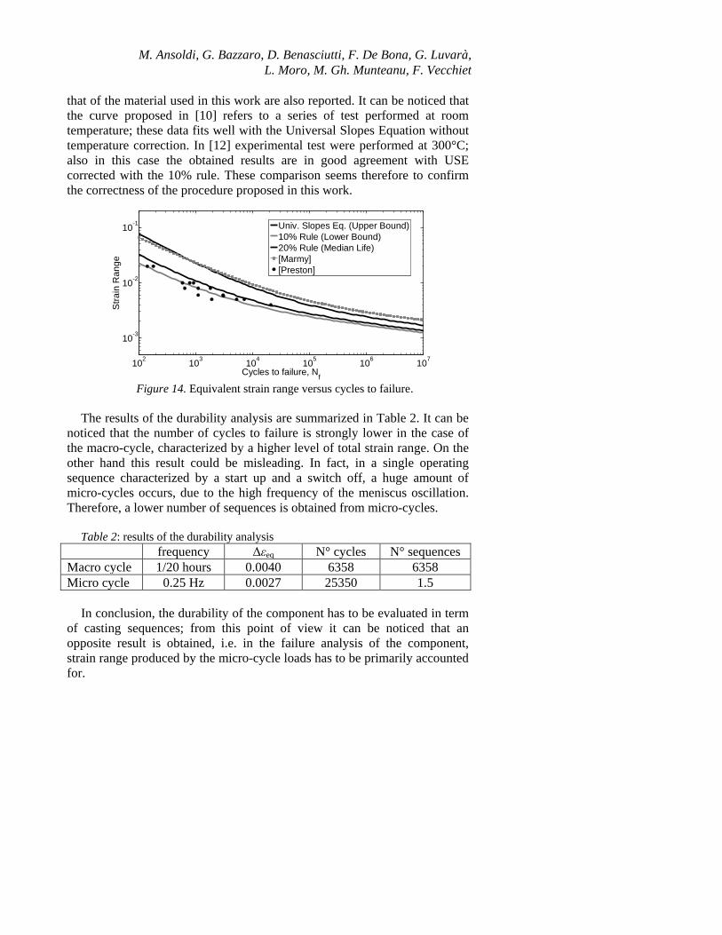
that of the material used in this work are also reported. It can be noticed that the curve proposed in [10] refers to a series of test performed at room temperature; these data fits well with the Universal Slopes Equation without temperature correction. In [12] experimental test were performed at 300°C; also in this case the obtained results are in good agreement with USE corrected with the 10% rule. These comparison seems therefore to confirm the correctness of the procedure proposed in this work.

102 103 104 105 106 107

10-3

10-2

10-1

Cycles to failure, Nf

Stra

in R

ange

Univ. Slopes Eq. (Upper Bound)10% Rule (Lower Bound)20% Rule (Median Life)[Marmy][Preston]

Figure 14. Equivalent strain range versus cycles to failure.

The results of the durability analysis are summarized in Table 2. It can be

noticed that the number of cycles to failure is strongly lower in the case of the macro-cycle, characterized by a higher level of total strain range. On the other hand this result could be misleading. In fact, in a single operating sequence characterized by a start up and a switch off, a huge amount of micro-cycles occurs, due to the high frequency of the meniscus oscillation. Therefore, a lower number of sequences is obtained from micro-cycles.

Table 2: results of the durability analysis

frequency Δεeq N° cycles N° sequences Macro cycle 1/20 hours 0.0040 6358 6358 Micro cycle 0.25 Hz 0.0027 25350 1.5

In conclusion, the durability of the component has to be evaluated in term

of casting sequences; from this point of view it can be noticed that an opposite result is obtained, i.e. in the failure analysis of the component, strain range produced by the micro-cycle loads has to be primarily accounted for.

41 7. CONCLUSIONS

This work deals with the thermo-mechanical analysis of a copper mould. The mechanical behaviour of the component under thermal loading condition is analyzed adopting a three-dimensional finite-element model, with the aim of performing an accurate evaluation of stresses and strains levels. Two critical zones have been detected, respectively in the hottest region of the inner surface (point A) and close to the corner (point B). An analytical structural model is then developed with the aim of performing a sensitivity analysis in the design phase. A curved beam model seems suitable to describe the stress distribution around the corner (point B). A hollow cylinder with an imposed temperature distribution fits the hydrostatic plane stress status observed at the mid-face surface close to the meniscus region (point A). Using static tensile tests data performed on specimens obtained from actual mould, durability curves have been obtained adopting the Universal Slopes Method. The values of the total strain ranges for the two stress-strain cycles that characterize the component operation have been finally evaluated, estimating the lifespan of the component either in terms of number of cycles and in terms of casting sequences.

The developed models could be a useful support for the prediction of the residual life in real operation if the tracking of the component load history is performed; moreover the effective evaluation of different design improvement strategies can be also achieved.

REFERENCES

1. J. K. Park, B.G. Thomas, I.V. Samarasekera. Analysis of thermomechanical behaviour in billet casting with different mould corner radii, Ironmaking and Steelmaking, 29:1–17, 2002.

2. A. Weronski, and T. Hejwowski. Thermal Fatigue of Metals, Marcel Dekker, New York, 1991.

3. J. K. Park, B. G. Thomas, I. V. Samarasekera, U. S. Yoon. Thermal and mechanical behavior of copper molds during thin-slab casting (I): plant trial and mathematical modeling. Metallurgical and Materials transactions, 33B: 1–12, 2002.

4. J. K. Park, B. G. Thomas, I. V. Samarasekera, U. S. Yoon. Thermal and mechanical behavior of copper molds during thin-slab casting (II): mold crack formation. Metallurgical and Materials transactions, 33B: 437–449, 2002.

5. I. V. Samarasekera, D. L. Anderson, J.K. Brimacombe. The thermal distortion of continuous-casting billet molds. Metallurgical Transactions 13B: 91–104, 1982.


6. T. G. O'Connor and J. A. Dantzig. Modeling the thin-slab

continuous-casting mold. Metallurgical and Materials Transactions, 25B: 443–457, 1994.

7. ITER Material Properties Handbook, ITER Doc. No. G 74 MA 9 01-07-11 W 0.2, Publication Package No. 7, 2001.

8. E. Winkler. Formänderung und Festigkeit gekrümmter Körper, insbesondere der Ringe. Der Civilingenieur, 4, 232–246, 1858.

9. S. Timoshenko and J. N. Goodier. Theory of elasticity. McGraw-Hill, 1952.

10. P. Marmy and O. Gillia. Investigations of the effect of creep fatigue interaction in a Cu-Cr-Zr alloy. Proc. Engineering 2: 407–416, 2010.

11. A. A. F. Tavassoli. Materials design data for fusion reactors. J Nuclear Materials, 258–263, 85–96, 1998.

12. S. D. Preston, I. Bretherton , C. B. A. Forty. The thermophysical and mechanical properties of the copper heat sink material intended for use in ITER. Fusion Engineering and Design 66 – 68, 441– 446, 2003.

13. J. H. You, M. Miskiewicz. Material parameters of copper and CuCrZr alloy for cyclic plasticity at elevated temperatures. Journal of Nuclear Materials 373, 269–274, 2008.

14. S. S. Manson. Thermal stress and low-cycle fatigue, McGraw-Hill, 1966.

15. J. A. Graham. Fatigue Design Handbook, Advances in Engineering, Vol. 4, Soc. of Automotive Engineers (SAE), 1968.

16. S. S. Manson, G. R. Halford. Fatigue and durability of structural materials, ASM International, 2006.

43

FAILURE ASSESSMENT OF TRANSMISSION DIODE LASER WELDED POLYPROPYLENE

E. GHORBEL, G. CASALINO, A. BEN HAMIDA

1 L2MGC- Univ. Cergy Pontoise, Neuville sur Oise – 95 031 Cergy Pontoise CEDEX – France

2 DIMeG, Politecnico di Bari, Viale Japigia, 182, 70126, Bari.

3Université Pierre et Marie Curie, Boîte 161, 4 place de Jussieu, 75 252 Paris Cedex 05, France

Email address:

1 [email protected]

2 [email protected]

3 [email protected]

Abstract: The aim of present work is to predict using finite element analysis the failure of polypropylene welded samples using the Laser Diode Transmission technique. The studied material is a commercial polypropylene (PP). The mechanical behaviour of the welded samples is modelled using elastic purely plastic law with a von Mises yield criterion. Both the thermal degradation and the heterogeneity of the weld zone were taken into account in the modelling, to approach the welding conditions and the geometry of the weld. The linear mechanic’s fracture was adopted to assess the failure of the welded samples. The assumption of the plane deformations is chosen to calculate the integral of contour of Rice “J” and to characterize the singularity of the stress field surrounding the weld zone. Good agreement is. The good agreement observed between the predicted and this experimentally obtained load failure suggests that our approach can be used as a tool for the prediction of failure of laser diode welded specimens.

Key words: polypropylene, diode laser welding, failure assessment.

mailto:[email protected]�



E. Ghorbel, G. Casalino, A. Ben Hamida 1. INTRODUCTION

Polypropylene (PP) is one of the most widely used polymers. The combination of low density, chemical resistance, low cost and a balance of stiffness and toughness allow thermoplastics to play a leading role and replace other materials in many important applications.

Two general forms of laser welding of plastics exist: direct laser welding and transmission laser welding. Direct laser welding usually uses CO2 laser radiation, which is readily absorbed by plastics, allowing quick joints to be made, but limiting the depth of penetration of the beam and restricting the technique to film applications. The shorter wavelength radiation produced by Nd:YAG, fibre and diode lasers is less readily absorbed by plastics, but these lasers are suitable for performing transmission laser welding. In this operation, it is necessary for one of the plastics to be transmissive to laser light and the other to absorb the laser energy, to ensure that the heating is concentrated at the joint region. Alternatively, an opaque surface coating may be applied at the joint, to weld two transmissive plastics. Transmission laser welding is capable of welding thicker parts than direct welding, and since the heat affected zone is confined to the joint region no marking of the outer surfaces occurs.

Among the properties of thermoplastics, deformation and ultimate tensile strength have revealed as a topical preoccupation in order to utilize them effectively in service applications, since almost every application, even the most trivial, involves some load bearing capability.

Therefore the increase in using polymer welds for several industrial applications leads to a strong need of developments of constitutive models. These models are based on either phenomenological or microscopic aspects. The purpose of this paper is to assess the influence of microstructure heterogeneity on the mechanical behaviour of polypropylene (PP) thermoplastics welded by diode laser.

The mechanical behaviour of flat samples under uniaxial load was studied by numerical and experimental approaches. The ultimate strength of a thermoplastic is naturally important in the matching of a material to an application, as with deformational properties. Some preliminary trials brought the authors to adopt the mechanics of fragile rupture as the most suitable law to predict ultimate tensile strength.

2. PROPERTIES OF PROPYLENE AND ITS WELD

Both pure polypropylene and 2% carbon black filled polypropylene were used in this investigation. The most important material properties related to these materials are summarized in Table 1.

45 Table 1: The most important material properties related to the welding behaviour of polypropylene. Obtained by DSC at 20°C/mn (Tg : vitreous transition, Tf : fusion et

Tc : cristallinization ). materials Tg (°C) Tf (°C) Tc (°C) Xc (%)

PP -18 170 110 31 PP (2%C) -16 173 112 33

The laser beam is totally absorbed within the surface (interfacial) of

carbon black filled propylene. Direct contact between the parts ensures heating of polypropylene at the joint interface. Welding occurs upon melting and fusion of both materials at the interface. The heating and melting of the polymer is started from absorbed energy black part.

50mmx50mmx3mm narrow plaques were used as sample geometry. Figure 1 shows the welding setup.

Figure 1. Welding setup.

Effects of the influence of laser power density and irradiation time

(welding speed) on the weld structure was investigated as well as the material parameters (black content) on weld soundness and heat affected zone and bead shape were performed [1]. From microscopic observations it appears that the cross section of the joining area has an elliptic geometry. The centre of the ellipse is located at the interface of both polymers. The increase of the laser power leads to a larger volume of the welding zone with a more important depth penetration. The increase of velocity conducts to a decrease in the volume of the welding zone that geometry remains elliptic

IR results as well as microscopic observations showed the thermal gradients produces an evolution of the cristallinity fraction along the cross

E. Ghorbel, G. Casalino, A. Ben Hamida section of the welding joint, a change on the morphology of the spherulites and the occurrence of a void due to the thermal decomposition and the vaporization of the polypropylene related to the presence of high temperature gradients in the seam. Hence, schematically, different zones in the welded part can be distinguished. In each zone, crystalline morphology is related to specific thermal cycle. The aim of this investigation is to study the influence of the microstructure and cristallinity rate on the failure of the welded samples loaded under uniaxial tensile conditions.

Several models can be used for the prediction of polypropylene weld failure: damage models, fracture mechanics, non-linear mechanics.

Uniaxial tensile tests were conducted on welded samples. The obtained results show that the behaviour of the specimens is linear until the fracture which was initiated in the proximity of the weld bead and developed into the black part (Figure 2).

0

50

100

150

200

250

300

350

400

450

0 0,2 0,4 0,6 0,8 1 1,2

déplacement(mm)

Forc

e (N

)

P=3,7 W

P=2,2 w atts

F

15 m

m

75 m

m

10 mm

F

Figure 2. Tensile test curve for a polypropylene weld obtained with 1,5 mm/s

welding speed.

3. MECAHNICAL MODEL OF THE WELD

Several works have dealt with the mechanical behavior of polypropylene. Uniaxial tensile tests show that the behavior is not linear at room temperature. The brittle-to-ductile temperature increases with increased cristallinity, which also increases the yield stress. Mechanical properties strongly depend on the cristallinity rate (Xc), the spherolite size (φ) and the molar mass (MW) [2, 3, 4]. Table 2 shows the quasi-linear relation between the cristallinity rate and the mechanical properties. More authors investigated the relation between the cristallinity rate and the PP rupture. [5, 6]. Plastic yielding and fracture influence the entropy change in

47 polypropylene through a significant change in the dissipation factor. An increase in crystallinity results in an increase in the entropy [7].

In this paper it was conceived that the mechanical behavior of the both transparent and pigmented layers can be described using an elastic perfectly plastic law with a Von Mises criterion (Eq. N°1). Material properties of each layer depend essentially on the crystallinity ratio Xc (table 2).

Table : PP properties against the rate of cristallinity [VAN 98 I et II].. XC (%) E (MPA) sσ (MPa) sε (%)

31 601 19.5 17.0 38 962 25.4 11.0 43 1228 31.9 8.8 53 1650 41.0 4.0

( )10

0 et : avec

eq s e

e p p

f Tr IE E

f ff d

ν νσ σ ε ε σ σ

σ ε ε ε ε λσ σ

•

+ = − ⇒ = = − ∂ ∂ = ⇒ = + =

∂ ∂

For transparent PP Xc=31% whereas different situations are considered

for the weld: the weld bead is assumed as a homogeneous and isotropic medium with Xc=37% and the weld bead is a heterogeneous medium decomposed on three homogeneous domains. Each domain is characterized by its own crystallinity ratio. The plane deformation condition was given to the weld in the proximity of weld bead, which tackled the singularity due to the domain change due to the different material properties. Rice integral was calculated at the point of singularity (J). In case of straight fissure and fragile crack « G » and « J » are connected by the following equation Ed. 2:

( )22

2 212

IIII II

KG J K K

Eν

µ−

= = + +

The tensile test was performed on a weld manufactured with Plaser=40 W

et Vlaser= 3mm/s. The heat affected zone was given an elliptic shape. The mesh was made up of 2° degree triangular elements. At the proximity of the weld bead the elements of the mesh were square.

The weld heterogeneity was modeled by means of three wrapping ellipsis. Each of three ellipses had different mechanical properties, as showed in figure 3.

Figure 4 shows the geometrical model of weld. A displacement along the x direction of 1mm during 10 seconds is imposed.

E. Ghorbel, G. Casalino, A. Ben Hamida

zone 3: E1= 650 Mpa, ν=0.35, σs=21 Mpa; zone 2 E2= 750MPa; ν=0.35; σs=23 Mpa; zone 1: E1= 850 Mpa, ν=0.35, σs=25 MPa.

Figure 3. Ellipsis with different mechanical properties.

Figure 4. Geometrical model of weld.

4. NUMERICAL RESULTS

Figure 5 shows the force (N) against the displacement (mm) during the simulation of the tensile test for two different set of the mechanical properties of the weld. It appears clearly that the microstructure inside the beam does not influence the response of the loaded welded samples.

Figure 5. Numerical simulation of the tensile test.

As a consequence the heterogeneity of the weld can be neglected. Figure

6 shows the Von Mises equivalent constraint. A bending phenomenon is noted corresponding to experimental observations.

Deplacement (mm)

Forc

e (N

)

49

The highest value of von Mises equivalent stress is detected inside the weld with a maximum located at the proximity of the seam leading to the highest equivalent plastic strain (figure 7). These results explain experimental observations during tensile tests consisting in the fact that fracture was initiated in the proximity of the weld bead and developed into the black part.

Figure 6. Von Mises equivalent constraint.

Considering that the restitution energy of the pure propylene is about 3

J/m2 [4] and that the black content reduces it, the rupture of the weld can be placed at 0.8 mm displacement, which correspond at a load of about 400N (see figure 8). The failure load obtained from finite element analysis is quite equal to that obtained experimentally.

0

0,5

1

1,5

2

2,5

0 1 2 3 4 5 6 7 8Distance à partir du centre du cordon (mm)

Défor

matio

n plas

tique

cumu

lée

0 1

Figure 7. Highest equivalent plastic strain.

5. CONCLUSION

The mechanical behavior of laser joined of polypropylene was investigated by numerical and experimental analysis. The numerical simulation of weld mechanical strength and rupture took into account the material heterogeneity, which depends on weld recristallization and the

E. Ghorbel, G. Casalino, A. Ben Hamida material degradation during the cooling phase of the thermal cycle, which causes also material lack.

The numerical results gave the idea that that heterogeneity can play a minor role in the mechanical strength and rupture of the weld. The displacement at fracture was calculated by means of the Rice integral.

The obtained results can be used for a deeper understanding of the PP weld mecahnical behaviour when deformation is due to a superimposed displacement.

REFERENCES

[1] Ghorbel, Casalino et Abed R. Characterization of thermal and mechanical effects of diode laser welding of Polypropylene. MATERIALS & DESIGN, Materials and Design 30 (2009) 2745–2751.

[2] Van der Wal A., Mulder J.J., Thijs H.A. et Gaymans R.J. “Fracture of Plypropylene : 1. The effect of molecular weight and temperature at low and high test speed” Polymer vol. 39 No. 22, pp. 5467-5475, 1998.

[3] Van der Wal A., Mulder J.J. et Gaymans R.J. “Fracture of Plypropylene: 2. The effect of crystallinity” Polymer vol. 39 No. 22, pp. 5477-5481, 1998.

[4] Avella, M. Dell’Erba, R., Martuscelli, E. et Ragosta, G. “Influence of molecular mass, thermal treatment and nucleating agent on structure and fracture toughness of isotactic polypropylene”, Polymer, Vol. 34, N° 14, pp. 2951-2960, 1992.

[5] Mareri, P., Bastide, S., Binda, N. et Crespy, A. “Mechanical behaviour pf polypropylene composites containing fine mineral filler: effect of filler surface treatment” Comp. Sci. Tech. 58, 747-752, 1998.

[6] Zebarjad, S. M., Tahani, M. et Sajjadi, S. A., “Influence of fillers particles on deformation and fracture mechanism of isotactic polypropylene”, J. of Mat. Processing Tech., article in press, 2004.

[7] T. Vu-Khanh, M. El Majdoubi. Entropy change with yielding and fracture of polypropylene. Theoretical and Applied Fracture Mechanics 51 (2009) 111–116.

51

Crack Tip Plastic Zone under Mode I Loading and the Non-singular Tzz-stress

Yu.G. Matvienko

Mechanical Engineering Research Institute of the Russian Academy of Sciences

Email: [email protected]

Abstract: The amplitudes of the second order terms in the three-dimensional series expansion of the crack front stress field are the terms xxT and zzT which describe in-plane and out-of-plane constraint, respectively. All previous analyses of the crack tip plastic zone have ignored the effect of zzT -stress. At the same time, the effect of

the zzT -stress on crack tip plastic zones is not revealed heretofore. It is therefore very important to obtain solutions for crack tip plastic zone size taking into account two components of the T-stresses. The present study focus on theoretical and numerical analysis of the joint effect of the non-singular xxT and zzT -stresses on sizes of the plastic zone in the vicinity of the crack tip under mode I loading conditions. The three-dimensional crack tip stresses including xxT and zzT stresses are incorporated into the von Mises yield criteria to develop an expression that models the crack tip plastic zone. Calculations are performed for three thicknesses of the CT specimen. The predicted sizes of the plastic zone in the vicinity of the crack tip of the analysed CT specimens are bounded by sizes of the plastic zones corresponding to two special conditions, namely, plane stress and plane strain. The theoretical results are compared with the results computed by FEM. Theoretical estimations of the plastic deformations zone size with provision for T-stress components in whole shows the satisfactory results, especially on line of the crack continuation. Key words: plastic zone, Tzz-stress, mode I crack


Yu.G. Matvienko 1. INTRODUCTION

The different sources of a change in in-plane constraint at the crack tip are associated with crack size, geometry of specimen and type of loading. The source of a change of the out-of-plane crack tip constraint is thickness. To describe in-plane and out-of-plane constraint effects in fracture analysis, the following parameters can be used, namely, zT -parameter [1], local triaxiality parameter h [2] and the non-singular terms in William’s series expansion of the crack tip stress fields [3].

These parameters considerably influence on the fracture toughness [4-8]. Not emphasize attention on advantages and disadvantages of the above-mentioned constraint parameters, we concentrate on the non-singular components of the T-stresses at the crack tip. The second order terms

xxT and zzT in William’s series expansion are defined as T-stresses, and they are the only non-zero and non-singular terms. It should be noted that

xxT has been simply referred to as T-stress. xxT and zzT represent the stresses in the crack surface plane normal to and tangential to the crack front, respectively.

In a two-dimensional (2D) crack configuration, zzT is related to xxT by

xxzz TT ν= under plane strain conditions, where ν is Poisson’s ratio. It is

well-known that the sign and magnitude of the xxT -stress substantially change the size and shape of the plane strain crack tip plastic zone [9-11].

Therefore, the xxT -stress has been used to characterize the effect of in-plane constraint on the crack tip plastic zone.

The amplitudes of the second order terms in the three-dimensional series

expansion of the crack front stress field are the terms xxT and zzT which describe in-plane and out-of-plane constraint, respectively. All previous analyses of the crack tip plastic zone have ignored the effect from zzT -

stress. At the same time, the effect of the zzT -stress on crack tip plastic zones is not revealed heretofore. It is therefore very important to obtain solutions for crack tip plastic zone size taking into account two components of the T-stresses.

The present paper focuses on theoretical and numerical analysis of the joint effect of the non-singular xxT and zzT -stresses on sizes of the plastic zone in the vicinity of the crack tip under mode I loading conditions.

53 2. THEORETICAL ANALYSIS OF THE PLASTIC

ZONE

2.1. Modeling of the plastic zone The general form of the linear elastic crack tip stress fields within a three-

dimensional crack problem can be characterized by the singular (the first order term) and the nonsingular terms (second order terms) [3]

...2

3sin2

sin12

cos2

++

⋅−⋅⋅

⋅= xx

Ixx T

rK θθθπ

σ , (1)

...2

3sin2

sin12

cos2

+

⋅+⋅⋅

⋅=

θθθπ

σr

KIyy , (2)

...2

cos2

2 ++⋅⋅

⋅= zzI

zz Tr

K θπ

νσ , (3)

...2

3cos2

sin2

cos2

+⋅⋅⋅⋅

=θθθ

πτ

rK I

xy , (4)

0=yzτ , 0=zxτ . (5) Here, r and θ are the in-plane polar coordinates of the plane normal to the crack front centered at the crack tip with 0=θ corresponding to a line ahead of the crack (Fig. 1), σ and τ are the normal and shear stress respectively, IK is the mode I stress intensity factor (SIF), E is Young’s modulus, ν is Poisson's ratio. The singular term corresponds to the stress intensity factor. The terms xxT and zzT are the amplitudes of the second order terms in the three-dimensional series expansion of the crack front stress field in the x and z directions, respectively. These terms characterize corresponding crack tip constraint along above-mentioned axes.

The xxT -stress component can be calculated from equations (1) and (2) as difference between xxσ and yyσ stresses very near the crack front. The

value of zzT -stress components is defined according to the following relationship [4]

xxzzzz TET ⋅+⋅= νε . (6) where zzε is strain along the crack front.

Yu.G. Matvienko

Figure 1: Three-dimensional coordinate system for the region along the crack front

In the case of plane stress conditions (2D stress state), stress

component 0=zzσ . For plane strain conditions, stress component zzσ is equal to

( ) xxI

yyxxzz Tr

K⋅+⋅

⋅⋅=+= νθ

πνσσνσ

2cos

22 . (7)

In the present work, the plastic zone ahead of the crack tip is determined by the von Mises yield criterion

( ) ( ) ( )( ) 2222

222

26 Yzxyzxy

xxzzzzyyyyxx

στττ

σσσσσσ

=+++

+−+−+−, (8)

where Yσ is the yield stress. Substituting of equations (1)-(5) into the von Mises yield criterion (8), the

crack tip plastic zone size prr = can be estimated. After comprehensive

mathematical manipulations, the solution for pr as a function of θ and the T-stress components is given by the following formula

22 22

1Yp

I

III

p

rKDAK

rσ

π=

⋅+⋅⋅

⋅ . (9)

55

The joint effect of the non-singular xxT and zzT -stresses on sizes of the plastic zone in the vicinity of the crack tip under mode I loading conditions is included into basic Eq. (9).

The parameters in Eq. (9) are denoted as follows

( )

⋅⋅+

+

+⋅⋅−⋅

+

⋅=

zz

zzxxxx

I

T

TTTD

2cos16

2cos8

25cos3

2cos

2 θν

νθνθθ

π, (10)

( ) ( ) ( )12cos43cos121 2 −⋅−+⋅−= θθνIA . (11)

Equation (9) can be solved to determine the angular distribution of the plastic zone size in the vicinity of the crack tip

[ ]2222,1 4

41)( WUVVU

rp ⋅+±⋅=θ , (12)

where parameters U, V, W are 24 YU σπ ⋅= , II DKV ⋅= , II AKW ⋅= 2

. (13) Finally, solution (12) can be written in more representative form

( ) 2

2

22

2

2

2,1162

16)(

⋅⋅

⋅⋅+±⋅

⋅

=Y

IYII

Y

Ip

ADDKrσπ

σπσπ

θ . (14)

It can be shown that special solution for the crack tip plastic zone in the case of plane strain conditions under mode I loading follows from general solution (12) (e.g., [11]):

24 TU σπ ⋅= , II EKV ⋅= , II BKW ⋅= 2. (15)

Here, the additional coefficients are

( ) ( ) ( )12cos43cos121 2 −⋅−+⋅−= θθνIB . (16)

( )

( )

⋅⋅⋅+

+⋅⋅−⋅

+

⋅=

xx

xxxx

I

T

TTE

νθν

θνθθπ

2cos16

22

cos82

5cos32

cos

2 . (17)

Yu.G. Matvienko

For plane stress conditions, the angular distribution of the plastic zone at the mode I crack tip can be calculated from (12) taking into account the following coefficients

24 TU σπ ⋅= , II FKV ⋅= , II CKW ⋅= 2, (18)

( ) ( )12cos43cos1 −⋅−+= θθIC . (19)

⋅

+⋅= xxI TF

25cos3

2cos

2θθπ

. (20)

It should be noted that equation (12) has to meet certain conditions, namely

04 22 ≥⋅+ WUV и 0≠U . (21) If above-mentioned inequalities (21) satisfy, sizes of the crack tip plastic

zone are calculated as

UWUVVrp 2

42

1

⋅++= , U

WUVVrp 242

2

⋅+−= . (23)

The value of 1pr is positive in the wide range of coefficients U, V, W and

should be used in all calculations. At the same time value of 2pr has a

negative sign.

2.2. The effect of thickness on the plastic zone For the 3D model, the CT specimen is considered. The plastic zone is

analyzed for a wide range of the ratio B/W=0.25-0.5 within the limits of the pure plane stress and pure plane strain conditions. The stress intensity factor Kmax of experimental specimens of Steel JIS S55C is 66 MPa⋅m1/2, corresponding values of the T-stress components are presented in table 1[7]. The T-stress components are calculated along the plastic zone boundary on the line of the crack extension. According with slight variation of the xxT -stresses for the CT specimens with different ratio B/W, the value of xxT -stresses has been assumed to be constant and equal to 182 MPa.

The fracture tends to initiate at the specimen thickness center, the values of the crack tip plastic zone size at specimen thickness center were chosen to represent the characteristic intensity of these values. The predicted results of the angular distribution of the plastic zone sizes in the vicinity of the crack tip at the specimen thickness centre for the CT specimens with various thicknesses to width ratio are given in Fig. 2. To determine the validity of the plastic zone model derived above, basic equation is applied to a pure

57 mode I situation under plane strain conditions, and the results agree with published solutions [9, 11].

Table 1: The T-stress components on the line of the crack extension (boundary of

the plastic zone) B/W 0,25 0,40 0,50

Txx, MPa 186.59 182.36 176.28

Tzz, MPa -159.47 -106.81 -84.97

Figure 2. The angular distribution of the plastic zone size at the specimen thickness centre of the CT specimens

The predicted sizes of the plastic zone in the vicinity of the crack tip of

the analysed CT specimens are bounded by sizes of the plastic zones corresponding to two special conditions, namely, plane stress and plane strain. Moreover, the shape and size of the plastic zones tend to typical plastic zones for plane strain conditions, when specimen thickness increases. Thus, the results confirm the necessity to take into account the constraint effect at the crack tip on the plastic zone by means of both non-singular stresses xxT and zzT .

Yu.G. Matvienko 3. NUMERICAL MODELLING THE PLASTIC

ZONE

3.1. Finite Element Analysis To demonstrate the validity of the plastic zone model, finite element

analysis was conducted.

Figure 3: The geometrical model of the CT specimen

It is well-known that the creation of the calculation model lies in the basis of numerical experiment. Primary tasks, which are being solved for this purpose, are the following. First of all, the solid-state geometrical model of the CT specimen (fig. 3) is created in the modern CAD system. Three geometrical models with the ratio B/W = 0,25, B/W = 0,40 и B/W = 0,50 are prepared for an analysis of the effect of the T-stress components on the plastic zone. Deviation from the figure was that the crack length a, was set at the nominal value of 12.5 mm (a/W= 0.5) for all cases.

The finite element model of the CT specimen is represented in Fig. 4. For the reason of minimization of the required computing resources finite element mesh was created on the one half of the geometric model (fig. 4). For more detailed account of the stress and strain distribution at the crack tip the local mesh concentration with diameter 10 mm was created around crack tip.

Spatial finite element mesh was created in one of the modern CAE system by means of decomposition of the internal volume of the geometrical model to the finite number of the small calculation elements having spatial polygon shape. Parabolic elements (the second order elements) with tetrahedral shape and one intermediate node along each side were used in this numerical analysis. The use of such elements allows achieving greater calculation accuracy due to more accurate

59 reproduction of the curvilinear surfaces of the geometric model, as well as more accurate shape function which connects displacement of the arbitrary point of the calculation element with displacement of its nodes.

(a) Two- dimensional global mesh

(b) Three-dimensional global mesh

Figure 4: Finite element model of the CT specimen.

The creation of the load system is made in the modern CAE system. Fixed values of the vertical forces (force P) were added to the nodes situated on the cylindrical surface of the specimen hole. The value of Kmax in the table 2 was obtained as the stress intensity factor corresponding to the maximum load Pmax from the well-known equation in ASTM E399.

Table 2: Loading conditions of the CT specimen B/W=0,25 B/W =0,40 B/W =0,50

Pmax, kN 6,0 9,6 12,0

Kmax, MPa⋅m1/2

66,0 66,0 66,0

Yu.G. Matvienko

Finite element calculations allow analyzing size and shape of the plastic

zone in the vicinity of the crack tip by means of diagrams of the von Mises equivalent stresses. 3.2. Algorithm for the processing of results of the numerical modeling

Sizes and shape of the plastic zone were analyzed using the image data of the distribution of equivalent von Mises stresses in the vicinity of the crack tip.

Estimation of the influence of the T-stress components on the plastic zone size is made in the mathematical package, for what special algorithm is created for processing the computed diagrams (Fig. 5). These diagrams must satisfy certain graphic conditions. The diagram must present itself as monochrome images of the equivalent stress fields with clear gray gradation of stress from white (stress level equal to yield stress σY) to black (zero stress level). In according with the main idea of algorithm the special procedure realizes consequent selection of pixels, which belongs to the image of the current diagram, along radius from the crack tip with appropriate step. If the color of current pixel differs from white, the procedure of pixel selection is stopped and current values of radius and angle are saved. This radius corresponds to the boundary of the plastic zone in the vicinity of the crack tip.

Figure 5: Typical image data of the distribution of equivalent von Mises stresses in

the vicinity of the crack tip of the CT specimen

4. DISCCUSSION

In according with the above-mentioned methodology for theoretical estimation of the plastic zone size, the predicted results are compared with the results computed by FEM. Comparison of theoretical and FEM results of the plastic zone size estimation at the CT specimen thickness is presented at Fig. 6.

61

Figure 6: Comparison of theoretical and FEM results of the plastic zone estimation

at the CT specimen thickness

It is observed that deviation of the theoretical plastic zone sizes from the FEM results does not exceed 20% in angular intervals (0°, 30…45°) and (90°…100°,135°…145°) (Fig. 7). Deviation achieves maximum and exceeds 40% in angular intervals from 135°…145° to 180° that can be connected with particularity of the algorithm which is used during processing of the equivalent von Mises stress diagrams.

Figure 7: Deviation of the theoretical plastic zone sizes from the FEM results

Yu.G. Matvienko

Probably, so high divergence between results of the numerical experiment

and analytical calculation in interval (0°…145°) can be explained that actually Т-stresses are not a constant and depend on angle θ. This assumption is corroborated by the results of the FEM analysis (Fig. 8, Fig. 9).

Figure 8: Finite Element estimation of angular distribution of the Txx-stress along the

boundary of the plastic deformations zone at the specimen thickness centre

Figure 9: Finite Element estimation of angular distribution of the Tzz -stress along

the boundary of the plastic deformations zone at the specimen thickness centre

63

We can receive evidence that dependence between T-stress components

and angular coordinate exists if we will express KI from equation (2) and substitute received relation to the equation (1). As a result we will receive angular distribution of xxT :

−

+⋅−=

25cos

2cos5

25cos

2cos3

θθ

θθ

σσ yyxxxxT . (27)

In similar manner we can receive angular distribution of zzT :

+

−⋅−= xxyyzzzz TT

25cos

2cos5

2cos8

θθ

θ

σνσ . (28)

Received relations confirm made early assumptions about necessity of the introduction into asymptotic formulas (1) and (3) angular distributions of components of the nonsingular stresses.

5. CONCLUSIONS

The theoretical analysis of the joint influence of the nonsingular components of the T-stresses on the size of the plastic deformations zone at the tip of the mode I crack is carried out with attraction of asymptotic formulas, which taking into account triaxiality of the stress state at the tip of the mode I crack and Mises yield criterion.

The size of the plastic zone at the middle surface of the specimen decreases during increasing of the specimen thickness. It reflects the increasing of the deformations constraint degree at the crack tip by means of increasing of nonsingular stress zzT .

Theoretical estimations of the plastic zone size with provision for T-stress components in whole shows the satisfactory results, especially on line of the crack continuation. This is especially important in case of estimation of the reliable values of the fracture toughness. However, in some cases divergence between analytical calculation and FEM results exceeds 20%. For more correct determination of the shape of the plastic deformations zone it is necessary to take into account angular distribution of the nonsingular T-stresses at the crack tip.

Yu.G. Matvienko

Certainly, accurate analysis and estimation of the plastic zone sizes at the mode I crack tip will promote the development of more correct criterions of validity in estimation of the fracture toughness of engineering materials.

REFERENCES

1. W. Guo. Three-dimensional analyses of plastic constraint for through-thickness cracked bodies. Engineering Fracture Mechanics, 62: 383-407, 1999.

2. B.S. Henry and A.R. Luxmoore. The stress triaxiality constraint and the Q-value as ductile fracture parameter. Engineering Fracture Mechanics, 57: 375-390, 1997.

3. T. Nakamura and D. M. Parks. Determination of elastic T-Stress along three-dimensional crack fronts using an interaction integral. International Journal of Solids and Structures, 29:1597-1611, 1992.

4. W.A. Sorem, R.H. Dodds and S.T. Rolfe. Effects of crack depth on elastic plastic fracture toughness. International Journal of Fracture, 47: 105–126, 1991.

5. S. Liu and Y.J. Chao. Variation of fracture toughness with constraint. International Journal of Fracture, 124: 113-117, 2003.

6. X.K. Xhu and Y.J. Chao. Specimen size requirements for two-parameter fracture toughness testing. International Journal of Fracture, 135: 117–136, 2005.

7. T. Meshii and T. Tanaka. Experimental T33-stress formulation of test specimen thickness effect on fracture toughness in the transition temperature region. Engineering Fracture Mechanics, 77: 867-877, 2010.

8. H.M. Meliani, Yu.G. Matvienko and G. Pluvinage. Two-parameter fracture criterion (Kρ,c-Tef,c) based on notch fracture mechanics. International Journal of Fracture, 167: 173-182, 2011.

9. J.R. Rice. Limitations to the-scale yielding approximation for crack-tip plasticity. Journal of the Mechanics and Physics of Solids, 22: 17-26, 1974.

10. S.G. Larsson and A.J. Carlsson. Influence of non-singular stress terms and specimen geometry on small-scale yielding at crack tips in elastic-plastic materials. Journal of the Mechanics and Physics of Solids, 21: 263-278, 1973.

11. Q. Nazarali and X. Wang. The effect of T-stress on crack-tip plastic zones under mixed-mode loading conditions. Fatigue and Fracture of Engineering Materials and Structures, 34: 792–803, 2011.

65

FAILURE ANALYSIS OF A STORAGE PUMP SHAFT

Niculai PASCA, Liviu MARSAVINA, Sebastian MUNTEAN, Radu NEGRU

Affiliation: 1) “ Politehnica “ University Timisoara, 2) Romanian Academy , Timisoara Branch


Abstract: The shaft is an important component in hydraulic pumps used to transmit power from electrical motor to the pump impeller. The paper presents failure analysis of a shaft, from a double suction hydraulic pump in operation of approximately 30 years, in a storage station. The shaft material is a Romanian steel, equivalent after their chemical composition and mechanical characteristics with American SAE 4340 steel for which in literature are available necessary data for failure analysis. The paper is structured in two parts: finite element analysis of the pump shaft and an analytical failure analysis for a circumferential crack type, using the failure assessment diagram (FAD). In a modeling program for stress and strain analysis the 3D shaft was loaded in torsion. The numerical results show the maximum stress zones, the stress concentration effect, and the possibility of crack occurrence. For circumferential crack type the failure assessment diagram for Mode III loading were plotted using the stress intensity factor solution. The results indicate the unsafe zone respectively the critical circumferential crack depth, where the shaft cannot operate with defects. This study presents an opportunity related to safe operation condition and remaining life estimation for a storage pump.

Key words: finite element analysis, stress, storage pump shaft, failure assessment diagram (FAD)


N. Pasca, L.Marsavina, S. Muntean, R. Negru

1. INTRODUCTION

Storage pumps all over the world are integrated equipment in hydropower facilities. These pumps are required to allow primarily large flow rate, in addition to operate at high efficiency and tolerant cavitation conditions. In Figure 1 is shown the cross section and the storage pump components: 1 impeller, 2 suction elbow, 3 volute, 4 shaft, 5 radial bearing , 6 radial-axial bearing.

Figure 1. Storage pump cross section.

Table 1: Technical characteristics of the storage pump

Parameters Symbol Value Pumping Head H [m] 197

Flow rate Q [m3/s] 4

Hydraulic Power P [kW] 8840

Efficiency η [%] 87.5

The pump shaft fails after approximately 30 years of operating time. In Figures 2 and 3 are presented the shaft fracture surface zone compared with theoretical aspect of a shaft failure in torsion loading condition [1]. This leading to hypotheses that shaft failed in torsion loading condition. In literature other studies present aspects of shaft failure in operating condition [2], [3], and [4]. In [2] the authors present a numerical turbine shaft failure

67

analysis with a crack propagation analysis using ANSYS and Afgrow software. An analysis of the premature failure of two counter shafts used in centrifugal pumps for lifting slurry has been carried out by Das et al. [3]. A collection of pump shaft failures like, corrosion failures on shafts, fatigue failures on shafts and shaft sleeve failures are analyzed [4]. However, these papers have not tackled the failure analysis using failure assessment diagram in mode III.

Figure 2. Fracture surface of the

investigated shaft. Figure 3. Sketch of fracture surface in

torsion loading condition [1]. This paper is structured in five parts which include a problem introduction, the shaft material, a stress and strain numerical analysis, and mode III failure diagram for a circumferential crack in a shaft. The conclusions are drawn in last section.

2. STORAGE PUMP SHAFT MATERIAL

The shaft material is a Romanian steel named after STAS 791-66, 34MoCN, with the following chemical composition presented in table 2. Table 2 Chemical composition and mechanical characteristics according to STAS 791-66 [5] for storage pump shaft material.

Steel name Chemical composition [%]

34 MoCN 15

C Si Mn Cr Ni Mo

0.3-0.38 0.17-0.37 0.4-0.7 0.6-1.7 1.4-1.9 0.15-0.3

Mechanical characteristics Yield Stress σy [MPa] Tensile strength σr [MPa]

882.9 1079.1


Material properties and specially fracture toughness are necessary for

failure analysis. Because for the Romanian steel these parameters are not presented in literature, and equivalent steel was searched. In table 3 are presented the material characteristics of the equivalent steel SAE 4340 [5]. It can be observed the chemical composition for both materials are very close. Table 3 Chemical composition and mechanical characteristics for equivalent steel SAE 4340 [6]

Steel name Chemical composition [%]

SAE 4340

C Si Mn Cr Ni Mo

0.37-0.4 0.23 0.7 0.7-0.9 1.83 0.2-0.3

Mechanical characteristics Yield stress σy[MPa] Tensile strength σr[MPa]

834 931 The fracture toughness for mode III of 4340 steel which is used in failure

assessment diagram for mode III construction KIIIc =68.235 MPa√m is presented [7].

3. STRESS AND STRAIN ANALYSIS

The stress and strain analysis for 3D geometry obtained in modeling software has been performed. The 3D shaft geometry is shown in Figure 4. Using the numerical software ANSYS has been performed a finite element analysis for the shaft.

Figure 4. 3D shaft geometry

The shaft model has been meshed using tetrahedral elements type 3D

Solid 187, defined by 10 nodes having three degrees of freedom at each node: translations in the nodal x, y, and z directions. The element has plasticity, hyperelasticity, creep, stress stiffening, large deflection, and large strain capabilities. In radial bearing close the electrical motor, where the shaft has an important stress concentrator, a fine mesh was performed, using 2 mm elements size. For this type of mesh the finite elements number was

69

215045 and 361108 nodes. A detailed stress concentrator zone with mesh refinement is presented in Figure 5.

Figure 5. A detailed stress concentrator zone with mesh refinement

The boundary conditions have been made according to real loading form

technical data sheets. A torsion loading was imposed from electrical motor which is transmitted to pump impeller located on the shaft middle, marked Mt torque. Another condition was the impeller weight marked with Gr and bearings in shaft zones indicate in Figure 6.

Figure 6. The problem set-up

A convergence study for maximum equivalent stress was performed. For

the fine mesh with 428468 elements and 719492 nodes the solutions difference are 0.43% compared with the solution with lower elements and nodes number. In Table 4 are presented the results for 7 meshes with different number of elements and nodes, respectively.

Table 4. Solution convergence study

Simulation case number

Maximum equivalent stress [MPa]

Elements number

Nodes number

Error [%]

1 487.79 215045 361108

2 487.42 224145 376389 1.46


3 487.32 265452 445752 1.03

4 487.29 304121 510686 0.79

5 487.24 352145 591329 1.11

6 487.22 398456 669096 0.72

7 487.16 428468 719492 0.43

The stress and strain distributions on the pump shaft were obtained using

finite element method. As a result, the shear stress (τxy, τxz, τyz), maximum equivalent stress and deformation are presented in figures 7, 8 and 9, respectively.

Results obtained and the fracture surface aspect indicate in Figure 2, show that the fracture occurred in bearing zone after application of shear loading where there is a stress concentrator. The stress results show a maximum in that zone, the maximum equivalent stress as the normal and tangential components is 483.97 MPa. The shear stresses occurring in the concentrator are τxy=131.45 MPa, τyz= 278.78 MPa while τxz is negligible.

Figure 7. Equivalent stress results on the pump shaft

Figure 8. Shear stress results: general view and zoom of the region with

maximum value (A region)

71

Figure 9. Deformation distribution on the shaft

4. FAILURE ANALYSIS DIAGRAM (FAD)

The failure (or fracture) assessment diagram is an attempt at combining failure criteria based on linear elastic fracture mechanics and plastic collapse. This failure criterion is a function of two parameters Kr and Sr, which respectively quantify the elastic fracture component and the plastic collapse component. Kr and Sr for failure mode III were calculated using eq. (1). Curve that represents a limit of safe design is plotted in the coordinate system (Kr, Sr). The safe zone is considerate, the zone below the curve provided Kr and Sr in FAD diagram.

IIIcKIIIK

rK = and crS τ

τ= (1)

where KIIIc [MPa m0.5] is the material fracture toughness in mode III [3] and KIII [MPa m0.5] represents the stress intensity factor in mode III at different crack length calculated with eq. (2):

]mMPa)[b/a(IIIFcIIIK πτ= and (2)

]MPa[)cD(

tM

232-

2

=π

τ (3)

where FIII(a/b) is the factor which consider the b=D shaft diameter 170 mm and a uncracked zone radius [8], c crack depth for circumferential crack, τ shear stress eq. (3), Mt torque moment, τc yield shear stress y.c ττ 5770= [9].

The failure criterion for mode III is presented by 3 models function of plastic zone shape near the crack: Hult-McClintock, Cherepanov and Bilby-Cottrell-Swinden.

2/12rr )]}AB1()S([1{K +-= (4)

where B/A is ratio of the semi minor axis to the semi major axis of the elliptic plastic zone.

Eq. (4) is a generalization of this failure criterion, for a customization we have different type of plastic zone near the crack (circle when B/A=0, elliptic when B/A=1). In case of B/A=1, result Hult-McClintock failure


criterion for mode III. For B/A=0, eq. (3) results Cherepanov failure criterion. Another failure criterion for mode III, based on the Bilby-Cottrell-Swinden customization has the same form as Dugdale model as eq. (5) [10]:

2/1r

2rr )]2Sπsec(ln)π8[(SK = (5)

Based on these failures criterion and the concept presented above were carrying out different shaft circumferential crack depth loaded in mode III.

The failure assessment diagram represented in Kr and Sr coordinates and obtained from eq. (1) is presented in Figure 10.

From the failure assessment diagram is observed that for a circumferential crack depth in shaft loaded in mode III, for all 3 failures solution critical depth is 33 mm, after this circumferential crack depth the shaft is in unsafe zone.

Figure 10. Failure assessment diagram in mode III

For crack depth between 33 mm and 35 mm after Bilby-Cottrell-Swinden

and Hult-McClintock failure criterion the shaft is in a safe zone.

73

5. CONCLUSIONS

The paper investigates the failure of the shaft from double suction storage pump using numerical analysis and FAD diagram. The numerical analysis has shown a stress field as well as the deformation distribution. A stress concentration near to the lubrication channel of the bearing is highlighted by shear stress and equivalent stress distribution. The fracture zone aspect indicates a mode III loading produced by torque in order to pass the power from electrical motor to the pump impeller.

The FAD diagram for mode III was developed taking into account three different plastic zone shapes and was applied for circumferential crack. As a result, the three models predict different critical crack depths. However, the value of the maximum crack depth of 33 mm is could be considered the maximum allowable crack depth. The inspection periods could be estimated based on the previous data in order to prevent a catastrophic accident.

ACKNOWLEDGEMENT

This work was partially supported by the strategic grant POSDRU ID77265 (2010), co-financed by the European Social Fund – Investing in People, within the Sectoral Operational Programme Human Resources Development 2007-2013. Dr. Sebastian Muntean was supported by Romanian Academy program.

REFERENCES 1. Rusu O., Teodorescu M., Lascu-Simion N., Material fatigue. Calculus guide, 1, Ed. Tehnică, Bucharest, 1992. (in Romanian) 2. Bordeasu I., Popoviciu M., Marsavina L.,Voda M., Negru R., Pirvulescu L., Numerical simulation of fatigue cracks initiation and propagation for horizontal axial turbines shafts, Annals of DAAAM & Proceedings, 407- 408, 2009. 3. Das G., Sinha A.N., Mishra S.K., Bhattacharya D., Failure analysis of counter shafts of a centrifugal pump, Eng. Fail. Anal., 6:267-276, 1999. 4. Berndt F., van Bennekom A., Pump shaft failures - a compendium of case studies, Eng. Fail. Anal., 8:135-144, 2001. 5. *** Alloy steels and high alloy steels for machine building, STAS 791-66, 1966 (in Romanian) 6. Davis J.R. (Editor), ASM Specialty Handbook - Carbon and Alloy Steels, ASM International, Metals Park, OH, 1996.


7. Liu Shu, Yuh J. Chao, Xiankui Zhu, Tensile-shear transition in mixed mode I/III fracture, Int. J. of Solids and Struct., 41:6147–6172, 2004. 8. Khoo S. W., Karuppanan S., Stress intensity factor for cracks emanating from a shaft, J. of Appl. Science, 11(10):1839-1844, 2011. 9. Susmel L., Multiaxial notch fatigue, CRC Press, USA, 2009. 10. Unger D., Analytical fracture mechanics, Academic Press, USA, 1995.

75

RECOVERING OF THE MECHANICAL PROPERTIES OF A PEHD PLATE CONTAINING A NOTCH BY THE GRINDING TECHNIQUE

D. Sersab, M. Aberkane

Laboratoire d'Elaboration de Caractérisation des Matériaux et Modélisation LEC2M.

Mouloud Mammeri University of Tizi-Ouzou. PO BOX 17 RP. Tizi-Ouzou 15000

Email address: [email protected],

[email protected]

Abstract : In this work, we present a repair approach of HDPE pipes. We use for this goal, a single Edge notched tension (SENT) samples with different notches lengths. We observe, in the first part, that the shapes of the force displacement curve change when the specimen contains a notch comparing to the tensile test of the plates without a notch and in the second part that the area value of the specimens decreases with the increase of the notch length. This area under the force-displacement curve represent the material deformation potential and the decrease of this energy indicate that the material loss his deformation potential in the presence of a notch. The aim of our contribution is to propose a rehabilitation method of the material deformation potential based on the mater removal around the notch by the grinding technique. We show that the recovering of the deformation potential of the material is possible by using this method. We, also, show that the mechanical properties of the material are better when the grinding well is bigger. To finish, we propose a recovering efficacy criterion based on the determination of the optimal value of Wa (where a is the notch length and W is the width of the sample), at eight percent (80%) of mechanical properties recovering, beyond witch the rehabilitation is ineffective. Key words: HDPE, repair, notch, tension, recovering.


D. Sersab, M. Aberkane 1. INTRODUCTION

Transport pipe is an enclosure under pressure transporting of the fluids at

long distances. It is known as an adduction when it is intended for the transport of the large flows. It must resist to the internal pressures of the transported fluid and with the constraints of the ground in which it is hidden. The transport pipes are manufactured with concrete, cement asbestos, cast iron, steel, PVC or HDPE. The canalization safety is one of the public interest and a question of the first importance. The number of fractures per year is a criterion of the pipe reliability. The presence of the defects in a pipe is unavoidable. These defects can be internal such as microscopic cracks, pores, the brittle particle's inclusions, or external due to the presence of notch (macro cracks) resulting from the process of construction, a corrosion or a damage caused by thirds . When the state of the defect is not sufficiently serious to lead to a complete replacement of pipe, and if the conditions of flow remain satisfactory, the rehabilitation of the pipes is justified. The state of the canalization, the possibility of action and the cost of a probably reparation are the element which are considered in the choice of the rehabilitation technique:

2. ANALYZE EXISTING DEFECTS IN A PIPE The analysis of the defects met in a pipe, enables us to use the following working hypotheses:

1. The defects, whatever their natures, are a geometrical discontinuities being able to be described simply by a notches which can be characterized by three parameters, the length a, the ray ρ and the angle of notch ѱ.

2. Under solicitation, the notches lead to a local stress concentration.

In the case of HDPE pipes, the defects are induced by stress concentrations generated by the presence of external or interior defects (scratches, stripes, scratches and inclusions) caused during the process of extrusion or at the time of the implementation of the canalization by wrong movement. For example, a wrong movement during the handling which can cause a geometrical discontinuity at least visible on the external surface of the pipe [1 ; 2]. These stress concentrations generate, according to conditions' of temperature, loading, depth of notch and environment various types of propagation of crack, such as the slow propagation of crack (SCG:slow fox trot ace growth).This type of progression, which results from the creep or the loading of tiredness, is wished the least because it does not show any sign before the rupture of the tube [ 3 ].It can be ductile or fragile.Lu and Brown [ 3 ] suggested that the two processes occur simultaneously;and the rupture final depends on which process is faster under the loading, the temperature and the depth given of notch. To evaluate the behavior of the PEHD under the quoted conditions known

77 several work is completed [ 3]-[4 ] and [ 5 ]; according to American Water Works Association the scratches which have a depth of 10 % thickness of wall of the tube in PEHD are tolerable [ 5 ] and above these 10% the product should not normally be used [ 6 ]. To give in service the tubes in PEHD presenting of the defects the PPI (Plastics Institute Pipe) published a technical note describing the various methods of repair according to characteristics' of the defect [ 7 ].

In this presented work we use the plates instead the pipe for obvious practical reasons. We chose the sample shape with Single Edge Notched Tension (SENT) because of the test simplicity and the possibilities that this geometry permit us in terms of repair by grinding or removal of matter.

3. PROPOSAL FOR TECHNICS OF REPAIR OF THE HDPE PIPE

A. Grinding reparation The problem of stress concentration being related to the notch effect, we

propose in our study a solution based on the modification of the shape of the notch. This solution consists on the reduction of the strong stress concentrations by the removal of adjacent matter at the least forced zones.

Figure1. Removal matter technic’s schematization [8]

This geometry treatment improves the profile of the defect by

eliminating the existing cracks and by reducing the related stress concentration.

4. EXPERIMENTAL METHOD

The samples used are rectangular (see figure 2), They are tested in uniaxial traction for the law of behavior of the virgin sample (1), the notched ones (2) and the repaired ones by the grinding technics (3). These samples are taken on HDPE pipe, with external diameter of 600 mm and thickness of 30 mm in the circumferential direction (see figure 3), The notch is practiced in the direction of extrusion, Sample's dimensions are in conformity with standard ESIS [9] which stipulates that in the goal to have a

D. Sersab, M. Aberkane planes stress in the ligament, it is necessary to observe the double following condition:

33 Wlb ≤≤ (1)

Figure2. sample used for the tensile test ;(1) : virgin sample; (2) : notched sample; (3) : sample repaired by grinding

Figure 3. Sampling direction

Figure 4. SENT Sample [4]

79

Table 1: Samples Dimensions

N° samples

Length l(mm)

Width

W(mm)

Thickness b(mm)

Length of notch

a (mm) 1

150 45 6

5 2 10 3 15 4 20 5 25

The tests are carried out on a IBERTEST tensile testing machine of +/-

100 kN load capacity. The forces and the displacements are measured by a load cell integrated into the machine and by a grip sensor directly posed on the sample respectively. The load-displacement curves are then collected and integrated by software into the machine in the form of Excel files.

5. RESULTS AND DISCUSSION

5.1. NOTCH'S INFLUENCE ON THE MATERIAL TENSILE BEHAVIOR

The notches carried out on the samples plainly change the material tensile behavior. We note that in the case of the virgin sample (see figure 5) we find the known behavior of the HDPE characterized by the succession of three stages which are:

1) The elastic phase with the thresholds of flow low and high; 2) The phase of flow elastic or viscoelastic; 3) The phase of hardening of material before its break off

In the case of the notched samples the viscoelastic phase disappears (see figure 5) and the elastic phase followed immediately the material break off. This indicating a great material embrittlement. This fact induces, also, a loss of a material deformation potential proportionally to the notch length.

Figure5. Curve load –displacement of the samples not notched (1) (black curve)and notched (2)(color curves)


5.2. PROPOSITION OF THE RECOVERING TECHNIQUE OF THE ELASTIC FLOW POTENTIAL

The material embrittlement observed previously is a problem and a proposed solution to avoid this situation is consisting on the total or partially recovering of the loss energy by rehabilitation or a repair technique. In our study we were inspired by the Eckstein [5] work who proposed a rehabilitation solution based on the removal of matter thanks to an operation of grinding of the cracked part (see figure 6).

Figure 6. principle of the grinding technique used

The principle of rehabilitation is very simple; it acts to grind the cracked area thanks to a wheel. To optimize this repair we use several diameters of a grinding wheel so as to be able to reach repair optimal. After the matter removal, we carry out tensile tests on the repaired samples and we compare the tensile diagram of the notched sample with that of the repaired samples (see figures 7 and 8).

Figure 7. Curve load-displacement of the samples repaired with radius of 5, 10

and 30 mm for notch’s depth a = 5 mm

81

Figure 8. Curve load-displacement of the samples repaired with radius of 25,

30 and 40 mm for a = 20 mm

We measure the material viscoelastic potential by the area under the tensile curve which is considered as the total energy dissipated during the notched sample fracture. We compare, then, this energy with the one dissipated during the tearing of the virgin sample. The test results are regrouped in a table which contain for each sample tested the notch length a, the grinding ray R, the maximum loading Fmax and the value of the area under tensile curve Wr.

Table2. Comparison of Fmax and W R before and after repair by

grinding

a [mm]

R [mm]

Wr [J]

Fmax [KN]

Before Reparation

after Reparation

before Reparation

After Reparation

Without notch

1240 1240 5.78 5.78

5

5 235.12 5.22 10 183.37 274.78 5.18 5.46

30 1192.50 4.69

10

5 210 4.73 10 132.09 333.52 4.35 4.45 25 373.91 4.60

15

5 92.32 130.56 3.54 3.54 25 309.40 4.14

20

25 140.05 3.25 30 62.65 625 2.72 3.35 40 617 3.37

25 306.58 2.7


25 30 39.36 580.57 2.03 2.58 40 1022.1 3.05

. We notice in table 2, on the one hand, that each time repair is undertaken

the Wr energy dissipated during tearing increases proportionally with the grinding ray, what indicates that grinding has a positive effect on the HDPE potential of deformation, in addition, we notice that the value of Wr drops proportionally with the length of the defect, These two observations, allow us to propose an optimum of repair which would take into account these two parameters.

1. REPAIR OPTIMIZATION

To account for the depth to which repair the notch could be effective we standardize all the values of energy of repair of the samples presented in table 1 at 60 mm of displacement, just at the necking end, we compare, then, the energy dissipated under the traction curve for the sample without notch (see figure 9) with the energy of the samples repaired, The results of these measurements are gathered in table 3:

Figure 9. Measure standardized energy of the healthy sample

Table 3: Table gathering the values of standardized energies of repair,

a [mm] [mm] L

[mm] Wrn [J] standardized to 60 mm of displacement [J]

0 0 0,00 267,84 5 30 33,17 207,41 10 10 20,00 200,11 10 25 40,00 210,13 15 25 45,83 182,77 20 30 56,57 143,45 20 40 69,28 150,89 25 25 50,00 122,83 25 40 74,16 131,60

83

To find the optimal value of repair, we plot a graph connecting the fracture energies standardized to a geometrical parameter which is report/ratio length of notch a over the ligament length W ( a/W ) as represented on figure 10,

0 0.1 0.2 0.3 0.4 0.5 0.60

20

40

60

80

100

a/w

Tau

x de

rec

ouvr

emen

t de

l'éné

rgie

initi

ale

(%)

Figure 10. Recovery rate of energy dissipation as a function of aspect ratio ( W/a )

In Figure 10, we note that the fracture energy of the material

decreasesWrn=267,84J corresponding to 100% of the energy is dissipated in the breakdown of the virgin sample Wrn= 207 J representing about 80 % for samples rehabilitated it then stabilizes between a ( a/W ) ratio ranging from 0.1 to 0.22 and then begin to decline until a rehabilitation rate of 50% of the energy dissipated. To optimize the repair we recommend a rehabilitation rate of energy dissipation of 80% which corresponds to an optimum aspect ratio a/W =0,22 beyond which the repair is not recommended and replacement of the section notched is recommended.

6. CONCLUSION

This work allowed us to shed light on the vulnerable behavior of HDPE in the presence of notches. It also allowed us to propose a solution for the rehabilitation of this material by the technique of grinding. The tests helped to highlight the influence of the grinding radius on the repair. It is shown that the material rehabilitation is better when the grinding radius is the largest. The close relationship between the ability to rehabilitate the material expressed by its ability to recover its qualities of plastic deformation expressed by its potential for dissipation of fracture energy normalized with the geometric properties of the samples expressed as the ratio ( a/W ) has determined an optimal value of this parameter at which the grinding repair method of HDPE is more efficient.

D. Sersab, M. Aberkane REFERENCES

1. A. Benhamena , L. Aminallah , B. Bachir Bouiadjra, M. Benguediab , A. Amrouche , N. Benseddiq “J integral solution for semi-elliptical surface crack in high density poly-ethylene pipe under bending ” Materials and Design 32 (2011) pp.2561–2569.

2. R. Schouwenaars, V.H. Jacobo, E. Ramos, A. Ortiz “Slow crack growth and failure induced by manufacturing defects in HDPE-tubes, Engineering Failure Analysis 14 (2007) pp.1124–1134

3. J. Zhang, “Experimental Study of Stress Cracking in High Density Polyethylene Pipes,” a Thesis Submitted to the Faculty of Drexel University by in partial fulfillment of the requirements for the degree of Doctor of Philosophy November 2005; pp.5-7.

4. D. Eckstein, “Buried Plastic Pipe Technology,” 2nd Volume, ASTM Special Technical Publication 1222 (1994).

5. Thomas S. Walsh, “Plastic Pipe and Fittings: Past, Present, and Future”, Journal of ASTM International, Selected Technical Papers STP1528 (November, 2011).

6. Plastics Pipe Institute, “Frequently Asked Questions; HDPE Pipe for Water Distribution and Transmission Applications,” Technical Note 27 (2009), pp 13; question 68.

7. Plastics Pipe Institute, “General Guidelines Repairing Buried HDPE Potable Water Pressure Pipes,” Technical Note 35 (2006).

8. A. Belalia, M. Aberkane et Z.Azari “La réhabilitation des canalisations de transport endommagées » Rapport CMEP tassili. Décembre 2010.

9. M. Aberkane, M. Ould Ouali “Fracture Characterization of ST37-2 Thin Metal Sheet with Experimental and Numerical Methods,” Key Engineering Materials. Trans Tech Publications inc. Volume 473, 2011, pp. 396-403.

85

SCENARIO OF FRACTURE DEVELOPMENT IN BUCKET WHEEL EXCAVATOR

Darko Daničić1, Stojan Sedmak2, Ivo Blačić3

1Kolubara metal, Lazarevac, Serbia 2University of Belgrade, Faculty of Technology and Metallurgy, Belgrade, Serbia 3Military Technical Institute, Belgrade, Serbia

e-mail [email protected]

Abstract: Continued service of BWE in the severe working conditions may result in machine failure. In case of important structural elements it might lead to a large-scale breakdown. The allocation of structurally significant elements is of vital importance for the lifecycle of BWE, starting from design and construction, through operation and maintenance. The example of recent failure of one BWE caused by complex fracture, consisting of fatigue and final fast fracture is considered. Possible scenario indicated that fracture started from a small element due to defects introduced by poor quality of welded joints which significance in structure was underestimated in given operating condition and applied loading. Key words: welding joint; stress distribution; structural integrity; maintenance


D. Daničić, S. Sedmak, I. Blačić

1. INTRODUCTION

In-service behavior of bucket wheel excavator (BWE) and other equipment operating on surface mines (bucket chain excavators, spreaders, belt wagons, stackers), aimed to supply electrical power plants by coal, depends on the design, capacity, manufacturing quality, applied loading and typical mining conditions (stability of mining area, strength of overburden mass, allowable soil loading). BWE development and application include design and manufacturing, acceptance for service after performed requested testing, operation, in-service inspection and maintenance. Structural integrity can be endangered in each of these steps, and this requires the decision to continue the operation or undertake the repair of damaged components. In spite of strictly obeyed prescribed rules and sequences, premature damages and failures of surface mine equipment occur in service, causing significant costs. Such failures are experienced also in opencasts surface coal mines in Serbia, and one of them is selected for a detailed consideration. In addition to direct costs, the losses due to downtimes caused by failure disturb electricity production, and for that they are important.

Performed failure analysis revealed that wheel with buckets and boom are most critical parts, requiring in some cases to improve the design /1-5/. One important aspect of excavator design is fatigue and fracture behavior of welded steel structures /6-8/. Welded joints, due to imperfections caused by manufacturing and heterogeneous microstructure (parent metal - PM, weld metal - WM, heat-affected-zone – HAZ) are most critical parts regarding crack initiation and growth, requiring special attention when exposed to variable loading and fatigue, as it is the case on open surface mines.

The service problems of equipment operating on surface mines attracted the attention and in many papers they had been considered /9-12/.

2. FAILURE OF A BUCKET WHEEL EXCAVATOR

To avoid unexpected failures of bucket wheel excavators (BWE) and save their structural integrity in service, necessary care during operational life, monitoring and diagnostics of all vital elements of supporting structure, sometimes also repairing and redesign, are required.

BWE SchRs 1760, unexpectedly and with no warning catastrophically failed in 2004, after 17 years of regular service, on an open surface mine in Serbia (Fig. 1). Fatigue fracture, initiated in welded joint and developed in lugs of counterweight holder (Figs. 2, 3), followed by final fast fracture, had been the cause. Cracks initiated in the sites of stress concentration and inhomogeneous microstructure of welded joints, primarily in HAZ, under the effect of external loads and residual stresses /13/.

87

Figure 1. Collapse of bucket wheel excavator SRs 1760

The fracture surfaces of left lug, pos. 68 (Fig. 3.a) and right lug, pos. 62

(Fig. 3.b) are substantially different. Right lug fractured in brittle manner, due to an overloading. Brute fracture in left lug took place when the loaded cross section area was significantly reduced after extended fatigue cracks on both sides of welded rib (Fig. 3). Flat fatigue crack growth in pos. 68 had been interrupted by stable crack growths, with visible shear lips.

Figure 2. Fracture of two lugs on counterweight holder

a.

b.

Figure 3.a. Lug (pos. 68) fracture (fatigue, stable crack growth and brute fracture) b. Brittle fracture of lug (pos. 62), indicating single initiation point from both sites

pos. 68

pos. 62


2.1. Analysis of applied load and stress distribution The loading acting on the bucket wheel is stochastic. It was limited

across the load cases given in the standard DIN 22261-2 /14/; sizing of individual components is done based on this standard. Based on the static load and center of gravity position, it can be seen that the anchor rope is exposed to the maximum load when the BWE is “ready to work” (load case in standard) with a horizontal boom. At the time of excavation, in any floor, the values of digging forces reduce, while the coupling slipped. Variable load and stress will be ranged between maximum and minimum values, i.e. between static load and minimum value, corresponding to maximum applied digging load in each digging contact between the bucket and the ground. This is confirmed by the strain alteration, recorded by strain gages (Fig. 4) /15/ in regular operating condition of BWE. When applied digging force exceeds nominal value for 50%, drive would be switched off automatically.

Analyzing the lugs in Fig. 2 and design scheme (Fig. 5.a) a symmetrical distribution of load and stress in two lugs could be assumed as reasonable. This was not the case, as it is possible to conclude analyzing the fracture surfaces on lugs 62 and 68 (Fig. 3).

Two effects could contribute to induced asymmetry. First one is an error in the design; the second one is low quality of welded joint, which allowed high level of stress concentration, induced by welding imperfection and defects. In this aspect it is necessary to explain (1) how cracks initiated and transferred from welded joint to lugs parent metal and (2) how variable loading and stress did not affect the behavior of lug, pos. 62 (Fig. 3.b).

0.00 0.20 0.40 0.60 0.80 1.00 1.20 1.40 1.60 1.80 2.00Time [Sec.]

-1.0

-0.5

0.0

0.5

1.0

Figure 4. Strains recorded in typical locations of BWE welded structure in operation

89

Figure 5.a. Design scheme of anchor ropes. b. Presentation of connection of the main rope and a structure of the counterweight

The design details of welded joint between rib (pos. 60) and the lug (pos.

68) are shown in Fig. 6. The same design is used for other lug, pos. 62. In the case of BWE SchRs 1760, originally applied design of connection

of the main rope to counterweight structure had more than one unfavorable solution. Double lugs design is used (Fig. 5) and the load distribution in structure is non symmetric regarding direction of the load. From Fig. 5.b it is clear that the tension force is transferred to the positions 62 and 68 through the ribs, pos. 60. In this way the distribution of load to the lugs is unbalanced. Ribs, although transferred the load, were treated as auxiliary elements and strict requirement for welding inspection was not prescribed.

Two facts have to be noticed. At first, the fatigue crack started from welded joint between the positions 68 and 60 (Fig. 7 left), on the defect location 1, produced by welding. Variable loading had been transferred as fatigue loading completely to position 68 (Fig. 3.a). On the other side, on the position 62, although similar defects had been detected (Fig.7 right), fatigue crack did not developed (Fig. 3.b). The explanation can be found in the design of the lugs: position 62 is fixed to the main structure (Fig. 5.b) while position 68 is free to swing.

pos. 62

pos. 68

pos.60


Figure 6. Design scheme of welded joint between lug (pos. 68) and rib (pos. 60)

Figure 7. Welded joints between rib and lugs (pos. 68, left, pos. 62 right)

Having in mind long time period for fracture, it is interesting to assess, at

least roughly, the time consumed for different steps. For that, the data recorded for BWE till its collapse is taken from the diary of work. They have shown total of 60 600 working hours with following data:

The frequency of load change 58.2/60 = 0.97 sec. The total number of load changes 60.600x3600/0.97= 2.25x108 The nominal circumferential force 373.8 kN The switch off force 560.7 kN Maximum calculated force in anchor rope 3874 kN

pos. 60

metal seam pos. 68

cross section surfice

view 1

view 2

91 2.2. Quality of welded joints

The design details (Fig. 6) indicate that fillet welds applied between rib (pos. 60) and the lug (pos. 68) had been performed without penetration, since the joint had been considered as an auxiliary one. These welded joints had not been manufactured according to welding procedure specification (WPS) and were not inspected properly. Heterogeneous microstructure (Fig. 8), and presence of defects and imperfections, (Fig. 9), discovered by investigation after collapse, are typical.

Figures 7 to 9 allow to conclude that for both lugs the welding quality is poor, causing eventually the high level of stress concentration, similar in joints of both lugs, pos. 68 and 62. to the ribs.

Figure 8. Welded joint section, normal to fracture of lug, pos.

68

Figure 9. Crack in the fillet weld root (up); incomplete root penetration (down)


3. PROBABLE SCENARIO OF FRACTURE DEVELOPMENT

3.1. Crack initiation in welded joint In BWE welded structure with defects (Fig. 7 and Fig. 9), and

inevitably heterogeneous microstructure (Fig. 8), exposed to load characterized by maximum initial static value and operational variable load, crack might be locally initiated by brittle fracture in microstructural region of low fracture toughness, by combined low cycle fatigue and crack tip blunting followed by stable crack growth in the more ductile region or by high cycle fatigue due to variable loading. Since the change in microstructure is sharp, crack initiation can include in both lugs all three, brittle, ductile and fatigue cracks, Fig. 7. The stress concentration, constraint and residual stresses, in addition to the variation of mechanical properties due microstructural heterogeneity can govern the mode of crack growth. Interrelation between influencing factor is decisive for the dominant type of a crack, but the fatigue crack will be surely present at the transition of welded joint to a lug, as can be concluded from Fig. 10.

Time period for crack initiation and propagation through weld metals in two runs (about 3,6 and 3,8 mm, Fig.) up to the HAZ of lug (2,2 mm) is difficult to evaluate because this process is complex.

Figure 10. Initiation of dominant fatigue cracks in lug, pos. 68: details in locations

A and B, LZ- ratchet marks, LO- beach marks, critical region C

93 3.2. Fatigue crack transfer to a lug

For the scenario of fracture in Fig. 3.a more interesting is development

of fatigue fracture in lug, pos. 68. More details about fatigue crack transition to the lug, pos. 68, are visible in Fig. 10. They might be used in explanation of fatigue crack initiation in this lug. Variable loading exerted its effect only to pos. 68, and not in pos. 62, what is attributed to fixation of the later to main structure.

Ratchet marks, beach marks and striations, as typical for fatigue, can be recognized on fracture surface (Figs. 7 and 10), which entered in lug as two separated fatigue cracks 1 in an early step and merged in a dominant fatigue crack 2 (Fig. 11). It is interesting to note that cracks 1 started in the HAZ of low fracture toughness in lug material, and crack 2 developed through the material of more homogeneous microstructure of parent metal.

Figure 11. Merged early fatigue cracks 1, points A and B, in a dominant crack 2

3.3. Advancement of fatigue crack

Continuous fatigue crack, above 300 mm long (Fig. 3.a), developed through homogenous microstructure, uniformly for every sequence of variable loading. In this segment of fracture Paris law can be applied for determination of time spent for fatigue crack growth.

Increasing fatigue crack continually reduced bearing cross section area of the lug, pos.68, to a size critical for fast fracture It is reasonably to assume that fatigue crack grew uniformly from crack 2, according to applied load, Figs. 3.a and 10, on both sides of welded joint, Fig. 7 left. Applied variable stress increased by increasing fatigue crack, due to continuously reduced bearing cross section area. This allowed fracture mode transformation from high to low cycle fatigue first, as shown in region IP and in magnified view in Fig. 12.


3.4. Stable crack growth by ductile fracture

Three regions of stable crack growth by tearing fracture had been registered in Fig. 3.a. They occurred when applied maximum stress in analyzed component locally exceeded yield stress of material, the energy had been consumed for tearing fracture and crack tip blunting, followed by shear lips and development of stretch zone, according to maximum shear stress, under 45° to acting force. But among these three regions there is the difference in starting condition. In the case on the left side (Fig. 3a) high cycle fatigue preceded stable crack growth, which had been arrested by final stretch zone (FSZ) in the region ZP. At the end of FSZ final fast fracture took place. On the right side, in the region IP (Fig. 12) low cycle fatigue preceded the tearing segment CA, which had been arrested by FSZ (Fig. 13). After this new FSZ, crack had to continue to grow, again by tearing fracture, up to the formation of FSZ before final fast fracture.

It is to notice that in all three cases plane stress dominated and shear lips are present. However, the sequence of occurrence individual tearing fracture regions is not clear and request further analysis.

Figure 12. Transition from flat fatigue

fracture surface, with visible beach marks and less visible striation, to stable tearing,

region IP in Fig. 3

Figure13. Final stretch zone after developed shear lips prior the next

stable growth of ductile crack, corresponding to region CA in Fig. 3

95

After stress redistribution, fatigue crack continued to grow continuously, by low cycle process beyond final stretch at CA and by high cycle process on the other side, up to simultaneous transition to tearing mode on both sides. Fracture process ended by fast fracture on both ends, after probably simultaneous development of final stretch zones (FSZ).

The region of transition from fatigue into static fracture is presented in Fig. 14. In addition to beach marks, static splitting fracture had been detected in the fatigue process, in crack tip blunting region, where structure with low cohesive strength are present along the plate thickness. The presence of static fractures on the fatigue fracture surface indicates the faster rate of propagation of the fatigue crack.

The presence of chevron patterns in the static fracture portion indicates the initiation of unstable growth, in the middle of plate thickness where plane strain condition dominated. Partial crack arrest (Fig. 15), along with unstable fracture, indicated that the fracture occurred above nil-ductility transition temperature (NDTT), in the brittle range. According to Pellini /16/, a material can arrest the crack only if the applied stress is lower than ½ Rp0.2. In this case, this is 185 MPa, well bellow allowed operating stress.

Figure 14. Transition from fatigue to

static fracture, PNL- final stretch zone Figure15. Crack arrest zone, ZP – crack

arrest

3.5. Final fast fracture of two lugs For final fracture it was necessary that applied stress exceed ultimate

tensile stress of material. The process of cross section area reduction took place during fatigue, but in fatigue stage only cross section of lug, pos. 68, had been affected, and not of pos. 62. During stable crack growth, which


preceded the final fracture, the reduction of cross section continued, still only of pos. 68. When total residual area of bearing cross section in both lugs had been reduced to a minimal value instantaneous fast fracture occurred, but by tearing mechanism. For the balance of applied load between different residual cross sections of two lugs, the load had to be redistributed, that means pos. 62 accepted greater part of the load than pos. 68.

This process had ended by development of first local final stretch zone CA. Simultaneously fatigue process might continue on lug other side up to the crack arrest and second final stretch zone ZP produced. When the stresses on both sides were balanced after strain energy had been consumed by final stretch zones development, last ductile stable crack had grown beyond CA location. This step finished by reached third final stretch zone. In this very moment bearing total cross section area of both lugs, pos. 68 and pos. 62, was reduced to the value critical for instant fast fracture.

The examination of the fracture surface of the position 62 showed the chevron pattern indicating that the fracture started in the weld metal, in the area between the two passes, Fig. 3.10. Generally, the occurrence of the unstable crack growth is typical for all the constituents of the welded joint and the parent material. Since no cracks have been arrested during the fracture of the position 62, one can say that, based on Pellini’s analysis /16/, the stress applied in the cross section was above ½ Rp0.2. This fracture has another typical characteristic: there are no shear lips on the fracture surface.

4. DISCUSSION

From theoretical point of view it is interesting to analyze the levels of applied stress and material response in different stages of considered fracture and the rates of crack growth, going back from final separation. This might help to better understanding of fracture mechanism and process duration.

Material will be separated if the applied stress exceeds ultimate tensile stress (UTS). However, it can happen at global level, for average value of applied stress, but also it can be sufficient if it happened locally, where stress concentration increases the value of average stress well above UTS. For tearing fracture the applied stress has to be in average higher than yield strength (YS) of material, accounting with stress concentration again. If the maximum value of applied variable load is slightly lower than YS, low cycle fatigue is most probable mode of cracking. The value of stress for high cycle fatigue should be lower than YS.

Rate of crack advancement also corresponds to fracture mode. For unstable fracture the rate is very high, the fracture occurred in very short time period, almost instantaneously. The rate of stable crack growth by tearing is lower, and for final separation, after final strength zone formation,

97 determined time is necessary. Low cycle fracture occurs in the range of cycle of variable loading (e.g. 50 000 to 100 000 cycles. For high cycle fatigue long time is required for crack development, measured by more than one million cycles.

It is also important to consider local microstructure for the evaluation of time necessary for individual steps of fracture.

The more detailed analysis of applied stress level, crack growth rate and microstructure investigation of welded joint is necessary for the evaluation of time period required for individual steps in presented fracture.

Roughly, of 17 years of BWE operation, it might be proposed that 70% of time had to be spent for high cycle fatigue, and the rest for crack initiation and early development in weld metal.

In the case of BWE fracture more interesting is practical engineering aspect of considered fracture, directed to the possibility how to avoid crack occurrence and how to prevent so difficult collapse and its consequences.

Fracture initiated from cracks in critical welded joint. The problem would not appear if this welded joint is not introduced in a structure of the counterweight. It is likely that, after experience with BWE failure, the design solution without welded joint of that kind is possible.

Next question is if the fatal collapse could be prevented by proper action during BWE design and exploitation.

By introduction of ISO 9000 series standards for quality assurance and ISO 9001 and ISO 9002 for quality systems welding is defined as "special process" because welded joints can not be fully inspected according to the standard requirements for a complete verification. In the case of welding, the quality can not be verified on the product but has to be built-in in the product. This generally accepted approach is dictated by the nature of fabri-cation in welding. Anyhow, the quality of welded joint can be endangered: (1) by defects induced during manufacturing and service and (2) by inevitable heterogeneity in microstructure and mechanical properties, corres-ponding to the nature of welding process, consisting of applied heating - cooling cycles.

In design stage most important was the underestimated significance of this welded joint, classifying it as auxiliary, and quality assurance system was not applied, neither in fabrication, nor in inspection. As a consequence, many detected defects and imperfections induced during manufacturing of welded joint contributed to high stress concentration, and critical welded joint was not available for inspection during service. In addition, misbalance of load and reduction of lug thickness from 40 mm to 20 mm by design solution produced inconvenient stress distribution. So, the structure contained the cracks, developed in fabrication or during operation under variable loading. For sure they could be detected in a proper inspection system, but it was not provided. Time period of 17 years of operation


indicates that in corresponding inspection and maintenance system the failure might be prevented.

5. CONCLUSION

Considering the importance of safe operation of BWE and other equipment operating on surface mines, complex systems for safety have been established, mainly as governmental agencies. It includes also welding procedures.

This approach is the direct contribution of new inspection and maintenance approach, especially proactive maintenance /17/, because the time estimates based on the crack can set a time frame in which the cracks can be detected and repaired to avoid a collapse of the structure. Also, during the inspection may be extended, reducing maintenance costs. Concerning this approach set a time in which critical elements of the structure should be revised so as to prevent damage, applying correct non-destructive examination. It means that corrected time of steel structure inspection can be applied basing on this kind of estimates and make more efficient inspection and maintenance.

Given the levels of assessment, definitely oblige to do the experimental confirmation of the hypothesis that would be a continuation of this work.

6. REFERENCES

[1] M. Arsić “Korelacija zamorne čvrstoće i praga zamora zavarenih spojeva” (“Correlation between endurance and fatigue threshold of welded joints”), Ph. D. thesis, Priština, 1995. [2] M. Arsić, S. Sedmak, M. Sarvan:“Analiza uzroka pojave prslina na zavarenim spojevima konstrukcije rotora bagera SRs 1300.26/5.0”, International conference “Welding 96”, Beograd, 1996. [3] D. Daničić, T. Maneski, D. Ignjatovic: Diagnostic approach to steel structure maintenance to prevent mining machine fractures, New Trends in Fatigue and Fracture, Metz 2010. [4] D. Daničić, T. Maneski, D. Ignjatović: Structural Diagnostics and Behaviour of Bucket Wheel Excavator, IVK 1-2010,53-60. [5] D. Daničić, T. Maneski: Structure Failure of the Discharge boom of BWE C 700 S due to Dynamic Effects, IVK 1-2012, 43-46 [6] M. Berković, Numerical Methods in Fracture Mechanics, IVK 2-2004, 63-66 [7] M. Berković, S. Maksimović, A. Sedmak, Analysis of Welded Joints by Applying the Finite Element Method, IVK 2-2004, 75-84

http://divk.inovacionicentar.rs/ivk/ivk10/ivk1001-6.html�



99 [8] T. Maneski, D. Ignjatović, Dijagnostika čvrstoće konstrukcije - Structural Performance Diagnostics, IVK 1-2004, 3-8 [9] T. Maneski, D. Ignjatović, Sanacije i rekonstrukcije rotornih bagera - Repair and Reconstruction of Bucket Wheel Excavators IVK 1-2004,9-28 [10] T. Maneski, D. Ignjatović, Sanacije i rekonstrukcije transportera i odlagača - Repair and Reconstruction of Belt Wagons and Stackers, IVK 1-2004, 29-38. [11] M. Arsić, S. Sedmak: “Spektar opterećenja za zamorna ispitivanja zavarenih spojeva rotornih bagera”, Međunarodno savetovanje “Zavarivanje ´94”, Novi Sad, 1994. [12] D. Daničić: Diagnosis of Conditions and Behavior for Steel Structures of Mining Machinery, PhD Thesis, Belgrade 2010. [13] S. Sedmak, V. Grabulov, D. Momčilović, Chronology of lost structural integrity initiated from manufacturing defects in welded structures, IVK 1-2009, 39-50 [14] Standard DIN 22 261-2:2006-12, Bagger, Absetzer und Zusatzgeräte in Braunkohlentagebauen - Teil 2: Berechnungsgrundlagen [15] N. Zuber, H. Ličen, A. Klašnja-Miličević: Applied Remote Condition Monitoring of the Bucket Wheel Excavator, Istraživanja i projektovanja za privredu, Naučno-stručni časopis, Beograd 2009. [16] W.S. Pellini, Guidelines for fracture-safe and fatigue-reliable design of steel structures, The Welding Institute, Abington, Cambridge, 1983. [17] P. Jovančić, D. Ignjatović: Proactive monitoring system for main mining mechanization at open cast mines, IVK 1-2010, 11-20.




101

ASSESSMENT OF THE BEHAVIOUR OF FATIGUE LOADED HSLA WELDED STEEL JOINT BY APPLYING FRACTURE MECHANICS PARAMETERS Ljubica Milović1, Srđan Bulatović2, Zoran Radaković3, Vujadin Aleksić4,

Stojan Sedmak5

1University of Belgrade, Faculty of Technology and Metallurgy, Serbia 2Yugoslav River Shipping, Belgrade, Serbia 3University of Belgrade, Faculty of Mechanical Engineering, Serbia 4Institute for Testing of Materials, Belgrade, Serbia 5Society for Structural Integrity and Life (DIVK), Belgrade, Serbia


Abstract: In discussion of the welded joints from fracture mechanics point of

view, it is assumed that the welded joint is pre-cracked and that therefore fatigue life of the pre-cracked structure is determined by the period of crack growth under variable loading. Experimental data obtained by testing provide a substantial foundation for better understanding and explanation of the phenomenon of fatigue of a material. Low-cycle fatigue (LCF) occurs during charging and discharging of the reactors, pressure vessels and pipelines; it can be accelerated by additional negative effect of temperature variation and aggressive effect of vessel contents during exploitation of the equipment in processing industry.

In present paper, the results of measurement of J-integral of weld metal made of low-alloy high-strength steel, used for manufacture of the pressure vessels in the process of powder welding, at LCF have been presented.

Keywords: LCF, J-integral, HSLA steel, process equipment

L. Milovi1, S. Bulatović, Z. Radaković, V. Aleksić, S. Sedmak

1. INTRODUCTION

Material fatigue can be clarified to a large extent using the results obtained by experimental examination, particularly so when one should understand the behaviour of a crack in a material with heterogeneous structure such as welded joint. Thus, we should conduct fatigue testing of fracture mechanics of the specimens with notch and crack for determination of the stress-intensity factor, KI and crack opening displacement, COD, or for determination of energy parameter, J-integral. In addition, one should compare conditions for crack propagation at high-cycle fatigue (HCF) and low-cycle fatigue (LCF) on one hand, and behaviour of the welded joint on the other hand. Based on it, one can get a picture of behaviour of the welded joint affected by fatigue loading, and the possibility of application of J-integral as a universal parameter of elastic and plastic behaviour of a material with a crack, and their effect on the problem of fatigue-crack propagation.

In present paper, measurements of J-integral at LCF for the specimens made of low-alloy high-strength HSLA steel (PM) and weld metal (WM) of their welded joints have been presented.

2. MATERIAL

For these tests, HSLA steel of NIONIKRAL 70B designation with welded joints made in submerged arc-welding (SAW) process with US-80B wire was chosen.

Chemical composition of tested material has been presented in Tab. 1 and chemical composition of the wire for the SAW process in Tab. 2, respectively.

Table 1 Chemical composition of tested batch of NIONIKRAL 70B steel (weight %)

C Si Mn Cr Ni Mo P S 0.19 0.4 1.11 1.06 2.59 0.25 0.019 0.024

Table 2 Chemical composition of US-80B wire for SAW of NIONIKRAL 70B steel (weight %)

C Si Mn Cr Mo P S 0.09 0.19 2.15 0.49 0.84 0.014 0.013

Tensile properties of HSLA steel of NIONIKRAL 70B designation have

been shown in Tab. 3 and tensile properties of WM of the welded joint weld in the SAW process with US-80B wire have been shown in Tab. 4.

Table 3 Tensile properties of NIONIKRAL 70B steel

Ultimate tensile strength,

MPa

Yield stress, MPa

Elongation A5, %

Reduction of cross section Z,

% 842 707 16 56.5

103

Table 4 Tensile properties of WM of tested welded joint

Ultimate tensile strength,

MPa

Yield stress, MPa

Elongation A5, %

Reduction of cross section Z,

% 848 701 17 46.2

3. PLAN OF THE EXPERIMENT

Welded plates, specimens to be cut from the plates, order of cutting of the specimens and their testing are defined by the work plan.

Experimental examination of the behaviour of NIONIKRAL 70B and WM of its welded joint included the following: 1. determination of the properties of PM and WM (the results have been

shown in Tabs 3 and 4); 2. determination of fatigue-crack growth at HCF; 3. measurement of compliance of a specimen and determination of

dependence of compliance and crack length; 4. establishment of dependence of fatigue-crack growth rate (increase of

crack length per cycle) and range of stress-intensity factor; 5. determination of JR-curve and critical value of JIC-integral, and 6. monitoring of J-integral value at LCF. According to the plan for cutting shown in Fig. 1, from two welded plates dimensions of which were 550 x 330 x 12 mm round specimens for tensile tests and CT specimens for testing of fracture mechanics were made.

Figure 1 Plan for cutting of CT specimens and specimens for tensile tests cut from

PM and WM of SAW welded joint

In this paper, the results of monitoring of J-integral value at LCF will be presented; other results can be found in [1].


4. THE RESULTS OF TESTING OF JR-CURVES WITH LCF PHASES

For application of HSLA steel in welded structures, its behaviour when affected by LCF is important, especially when a part of the structure contains a crack, [2-6].

4.1. TESTING OF SPECIMENS FROM PARENT METAL

CT specimens (B=11.85 mm; W=86 mm; a0=32 mm) from PM were tested for resistance to cracks based on JR-curves with phases of one-direction LCF for analysis of the effect of LCF on shape of JR curves and value of JIC. The data on testing of the subject specimen have been shown in Tab. 5.

As one can see from Tab. 5, testing was conducted in a few phases shown in Fig. 2. Taking into consideration noticeable proportion of LCF, in these tests residual strain, measured by the magnitude of residual COD, was monitored.

Figure 2 Fracture surface of CT specimen cut from PM

105 Table 5 Data on complex tests for determination of JR –curves with phases of LCF for CT specimens taken from PM

FATIGUE

COMPLIANCE

CRACK OPENING

DISPLACEMENT

(COD)

Test

pha

se

Upp

er fo

rce,

Fm

ax, k

N

Low

er fo

rce,

Fm

in,,

kN

R=F m

ax/F

min

Freq

uenc

y, f,

Hz

Incr

ease

, No.

of c

ycle

s, ΔN

,

cycl

e

Tota

l No.

of c

ycle

s,

N c

ycle

Incr

ease

, cra

ck le

ngth

, Δa,

mm

Tota

l cra

ck le

ngth

,

a, m

m

Max

stat

ic fo

rce,

kN

Res

idua

l, μm

Cur

rent

, μm

Tota

l, μm

Com

plia

nce

C, μ

m/k

N

A

32 50

408 408 8.16

32 70 576 576 8.23

32 30 67 244 311 8.13

32 50 67 408 475 8.16

B

36.1 5.1 0.14 26 5000 5000 2.7 34.7 70 67 597 664 8.53

50 5.7 0.11 1 300 5300 1.2 35.9 50 96 435 531 8.7

36.1 5.1 0.14 28 104 15300 2.02 37.92 30 96 280 376 9.33

C 4.18 42.1 89 96 3808 3904

D

40 2816 504 3320 12.6

32 4.8 0.15 21 2000 2000 0.5 42.6 40 2816 512 3328 12.8

32.2 5.6 0.17 21 5000 7000 1.8 44.4 40 2816 608 3424 15.2

32.2 4.8 0.15 21 5000 12000 3.1 47.5 40 2864 741 3605 18.53

32.2 4.8 0.15 21 5000 17000 3.8 51.3 40 2920 939 3859 23.46

40 4 0.1 0.9 100 17100 1.1 52.4 40 2934 1019 3953 25.74

E

53.6 45.5 2994 2568 5562

43.5 3.5 0.08 30 0.22 53.82 43.5 4426 160 4586

54.65 41.75 4558 2400 6958

35 5 0.14 18 0.4 55.05 39 5806 128 5934

F 24.9 5.3 0.21 20 4200 4200 9.35 64.4 10 5878 688 6566 68.8

G

0.7 65.1 18.75 5966 2760 8726

18.5 2 0.11 30 0.15 65.25 18 7454 152 7606

0.2 65.45 17.25 7482 2416 9898 74.3

H

11.25 1.25 0.11 20 5010 5010 4.05 69.5

8.7 0.85 0.11 20 2100 7110 7.3 76.8


A-static tension for determination of compliance; B-fatigue-crack propagation a0I with determination of; C-JR-curve; D-fatigue-crack propagation a0II with determination of compliance; E-JRII-curve with LCF phases; F-HCF; G- JRIII-curve with LCF phase; H-HCF

4.2. TESTING OF SPECIMENS FROM WELD METAL

The plan of testing of CT specimen (B=11.8 mm; W=86 mm; a0=32 mm) with a notch in WM differs from the previous one, as in this testing LCF has had the most important role. The data from this testing are presented in Tab. 6, but it should be noted that monitoring of the data on testing was stopped after the second LCF (R≈0.5).

5. DISCUSSION

5.1. TESTING OF SPECIMENS FROM PM

Starting compliance of the specimen with a notch in PM was determined by static loading (test phase A in Tab. 5).

Table 6 Data on complex tests for determination of JR –curves with phases of LCF for CT specimens taken from WM

FATIGUE

COMPLIANCE

Max

. sta

tic fo

rce,

kN

CRACK OPENING

DISPLACEMENT (COD)

Com

plia

nce

C, μ

m/k

N

Test

pha

se

Reg

iste

red

data

poi

nt

Upp

er fo

rce

F max

, kN

Low

er fo

rce

F min

,, kN

R=F m

in/F

max

Freq

uenc

y, f

, Hz

Incr

ease

No.

of c

ycle

s, ΔN

,

cycl

e

Tota

l No.

of c

ycle

s, N

cyc

le

Incr

ease

, cra

ck le

ngth

, Δa,

mm

Tota

l cra

ck le

ngth

, a,

mm

Res

idua

l, μm

Cur

rent

, μm

Tota

l, μm

A 1 32 35 242 242 6.93

B

2 36 3.6 0.1 25 200 200 0.5 32.5 35 252 252 7.2

3 33 3.3 0.1 25 27600 27800 1.5 34 35 261 261 7.46

4 33 3.3 0.1 25 14600 42400 2.4 36.4 35 280 280 8

C 5 4.1 40.5 88 944 915 1859 10.4

D

17 71 7.1 0.1 0.5 50 50 70 840 12

18 70.5 7.05 0.1 0.5 50 100 69 862 12.5

19 69 6.9 0.1 0.5 50 150 67 911 13.6

20 66 6.6 0.1 0.5 50 200 62 992 16

21 62 6.2 0.1 0.5 50 250 57 1049 18.4

107

22 57 5.7 0.1 0.5 50 300 54 1064 19.7

23 53 5.3 0.1 0.5 50 350 48 1113 23.2

24 46 4.6 0.1 0.5 50 400 41 1148 28

25 38 3.8 0.1 0.5 50 450 32 1145 35.8

26 27 2.7 0.1 0.5 50 500 21 61.5 19 1500 906 2406 47.7

E

27 19.84 9.9 0.5 0.5 50 50 22 1084 49.3

28 21.92 10.96 0.5 0.5 50 100 21.6 1080 50

29 21.52 10.76 0.5 0.5 50 150 213 1075 50.5

30 21.36 10.68 0.5 0.5 50 200 21.2 1087 51.3

31 20.96 10.48 0.5 0.5 50 250 20.8 1096 52.7

32 20.64 10.32 0.5 0.5 50 300 20.6 1092 53

33 20.16 10.08 0.5 0.5 50 350 20 1094 54.7

34 19.68 9.84 0.5 0.5 50 400 5.3 66.8 19.4 1800 1100 2900 56.7

F 8.2 75

A- static tension; B-HCF with determination of compliance; C-JR curve; D-LCF immediately after determine of JR curve; E-LCF R≈0.5; F-final HCF.

Residual strain at the point at which the data were registered, 3, resulted from exceeded yield stress limit and small extension of the root notch. In phase B, fatigue crack 37.92 mm-long was initiated, with initial and final HCF between which 300 cycles of LCF, designated in Fig. 2, were realized. Fatigue was interrupted from time to time, for measurement of compliance. After that, standard determination of JIC in phase C using JRI curve followed. Crack propagation in phase C was 4.18 mm and the value obtained, JIC = 212.78 kJ/m2, was in accordance with the results of previous testing. Upon completion of phase C, measurement of COD was resumed from zero (knife edges that support the gage arms were moved, as the full working range of the COD-measuring device of 4 mm was exceeded). It was then that testing of the specimen was interrupted for the first time. In the next phase, D, the specimen was again subjected to fatigue, with determination of compliance at intervals. After 4 cycles of HCF, 100 cycles of LCF followed. The specimen prepared in that way, with initial fatigue-crack length a02=52.4 mm, was subjected to complex testing, phase E, by applying monotonous loading and successive unloading.

5.2. TESTING OF SPECIMENS FROM WM

The testing started with three successive HCF, during which an increase of physical crack length of 4.4 mm was attained, so that static loading F-COD was conducted with initial fatigue crack of 36.4 mm. After sufficient number of unloading points for determination of the value of plane-strain fracture toughness was obtained, LCF was tested with minimum force – maximum force ratio R≈0.1. When the value of amplitude of upper force dropped below 20 kN, testing of LCF was resumed at R≈0.5. To mark

L. Milovi1, S. Bulatović, Z. Radaković, V. Aleksić, S. Sedmak attained crack length, we resumed with HCF until specimen fracture. In Fig. 3, the appearance of fracture surface is given, showing the differences in behaviour of WM induced by heterogeneous structure and existence of the defects. Face of the fatigue crack is blocked in development on one side, probably because of the existence of some defect in the structure (surface A in Fig. 3). That is why the crack face under static loading had the shape of an irregular triangle (surface B in Fig. 3), with clear flat fracture in the crack plane, that only after crack growth of 1.4 mm deflects at an angle of 45° in the direction of maximum tangential stresses (plane stress state). In initial phase of LCF, surface C in Fig. 3, the crack first propagates along the edges of the specimen, face line becomes more regular in shape and fatigue crack propagates, but still under conditions of plane stress state. The effect of the fusion line becomes apparent. Namely, at the side surfaces fracture develops at the boundary between heat-affected zone (HAZ) and WM. One should also observe the surface D, on which fracture is partially brittle due to structural defects in WM. HCF characteristic for the crack length shows similar fracture surface, and it is only in the final stage of fracture that shear lips forms again.

6. CONCLUSION

In present paper, experimental procedure for analysis of material crack resistance using the parameters of fracture mechanics for three types of effective loadings (HCF, monotonously increasing loading and LCF), as well as at combined loading (monotonously increasing loading with LCF phases), has been presented. By applying the above-specified loadings to PM of HSLA steel NIONIKRAL 70B and its WM obtained by SAW welding procedure, the properties relating to resistance of these two constituents of a welded joint were determined and compared. The values obtained, JIC≈210 kJ/m2 for PM and JIC≈90 kJ/m2 for WM, indicate degradation of the properties of the joint in WM. More inferior properties of the joint in WM are also indicated by decrease of the value of J-integral in the phases of LCF.

Acknowledgment. This experiment has been performed within the project TR35011 funded by the Republic of Serbia, Ministry of Education and Science, whose help is gratefully acknowledged.

109

Fig. 3 Fracture surface of CT specimen cut from WM

References

[1] Application of Fracture Mechanics Parameters for the Assessment of Welded Joint Behaviour in Conditions of Fatigue Loading, Doctoral Thesis Mohamed Ahmed

[2] ASTM E1823-11: Standard terminology relating to fatigue and fracture testing

[3] ASTM E606-04e1: Standard Practice for strain-controlled fatigue testing [4] ASTM E647-11e1: Standard test method for measurement of fatigue crack

growth rates [5] ASTM E813-81: Standard test method for JIC, a measure of fracture

toughness [6] Chow, C.L., Lu, T.J., Cyclic J-integral in relation to fatigue crack initiation

and propagation, Engineering Fracture Mechanics, 39(1), 1991, 1-20.

111

THE APPLICABILITY OF STRATEGY FOR RISK BASED MAINTENANCE TO A PENSTOCK

Tamara Sedmak1, Stojan Sedmak2, Ljubica Milović3

1University of Belgrade, Faculty of Mechanical Engineering, Serbia 2Society for Structural Integrity and Life (DIVK), Belgrade, Serbia 3University of Belgrade, Faculty of Technology and Metallurgy, Serbia

Email adress: [email protected]

Abstract: The risk of brittle fracture of pumping up penstock was recognized in an early stage of design. To reduce the cost of penstock construction one tunnel was accepted. For that most stressed penstock section HSLA steel, 700 MPa yield stress, 47 mm thick, was selected. Two problems were induced regarding brittle fracture. Cold cracks in welding could be avoided applying undermatching approach. This required to specify welding procedure and to qualify it for used thickness. Designed thickness might produce plain strain condition. For detailed analysis of cracks effect and stress state it was accepted to produce two full-scale prototypes of penstock most stressed part. Obtained results by fracture mechanics methods have shown sufficient crack resistance of PM, WM and HAZ in welded joints. It was necessary to assure structural integrity of welded joints and penstock involving corresponding approach for maintenance and repair. Maintenance procedures are in continuous development, and most promising is probably risk based approach, developed in last years. In the paper the base requirements of this approach are considered, and the possibility and convenience to apply them for penstock is evaluated. Key words: brittle fracture; welded joint; undermatching; penstock; prototype model; risk based maintenance


T. Sedmak, S. Sedmak, L. Milović

1. INTRODUCTION

Hydro-electrical power plant (HEPP) systems might require large amount of water in the Storage Lake and high fluid flow rate for the operation. For such a system the consequences of unexpected failure can be catastrophic, producing a great risk in service. In order to avoid the failure, preventing measures have to be applied /1/.

One of very important component in HEPP is a penstock, which can be exposed to high stresses, and for that be susceptible to failure. To reduce the risk level, operational safety of individual components in HEPP system, including penstocks, must be at very high level, This requirement comprises the assurance of high quality of produced components.

The failures of penstocks and pipelines are not frequent. Mechanical damages observed before and during service, fatigue, corrosion defects, welding imperfections and environment effect are referred as most important causes. Plastic collapse and brittle fracture are not cited often as failure cause, because applied steels for pipelines are ductile, and pipelines are used in the region above nil-ductility transition temperature.

However, cracks, brittle fracture and leakage had been experienced in penstocks produced of weldable high strength low alloy (HSLA) steels, developed and applied for reducing manufacturing costs by lower wall thickness /2/. Proof pressure test is required before acceptance for service, in some cases also testing of model is necessary.

2. EXAMPLES OF BRITTLE FRACTURE AND LEAKAGE

Two examples of failures /2/ are selected to illustrate the significance of risk analysis for penstocks. They also have shown the significance of welding procedure specification (WPS) for maintenance system and possible risk in service of a penstock.

Typical example of fast brittle fracture is catastrophic failure of penstock (length 2640 m, hydrostatic water pressure 864 m), occurred in 1973 year during pressure proof test in one knee close to machine house in HEPP „Santa Isabel“ in Bolivia. Failure occurred at pressure 735 m, e.g. at 84% of design pressure. Water jet passed through hole 1 m long and 0.7 m wide, and destroyed tropical vegetation along 130 m and 10 m in width. About 6000 m3 of water leaked for one hour, before the closing the valve in surge tank. The penstock was repaired by new segments for the knee. The tubes were produced of quenched and tempered steel Aldur 50/65D. This steel is designed for penstocks. In damaged knee pipe diameter was 1.15 m, plate thickness 22 mm. Mechanical properties, tested after failure, corresponded to specification. Metallographic examination revealed that failure cause is brittle fracture, initiated in the heat-affected-zone (HAZ) of longitudinal

113

welded joint, performed by sub-merged arc welding (SAW) procedure. Crack developed from the initiation point on both sides in the directions parallel to weld, and arrested at transversal manual arc welded joint, where continued to grow in direction normal to the weldment. It is evaluated that the possible failure cause is weld repair, since the preheating had not been applied according to welding procedure specification (WPS). Since involved steel is ductile, tough and crack resistant, the presence of high level of welding residual stress due to improper welding technology reduced penstock strength. After repair, in repeated test, penstock passed pressure 30% above design pressure, corresponding to 1170 m.

The next example, failure of penstock of „Peručica“, due to partial leakage, showed the significance of quality assurance in welding. Neither brittle fracture nor complete leakage occurred, but the occurrence of cracks in welded joints required measures for preventing of the break of power plant operation. Cracks occurred in welded joint of a ring, 100 mm wide, consisting of 6 circumferential segments (pos. 104 in Fig. 1). The diameter of penstock (pos. 103 left) is reduced from 4000 mm to 3400 mm in inlet line for turbine (pos. 103 right). Two pipelines were produced by different manufacturers, and significant misalignment and end distance occurred, what was solved by the collar (pos. 105), welded before the ring and accepting the loading by fillet welds. The ring served to fill the gap. After welding, the tunnel was filled with the concrete outside penstock, and penstock was protected inside by lacquer. Steel of 450 MPa yield stress, microalloyed by vanadium, was selected for collar and ring. After 10 years of service numerous cracks were revealed, several hundreds millimeters long, in both ring welded joints „A” and „B“ (Fig. 1), some of them passing through the weld and reaching fillet weld of pos. 105, i.e. the space between collar and ring. During the examination of empted penstock the water was found in cracks, confirming that crack depth reached the thickness of the ring, i.e. tube. The monitoring of cracks showed that they did not grow, or grow slowly.


Figure 1. Design of collar (pos. 105) and ring (pos. 104) for joining the penstock

Examination had shown that cold cracks are in question, occurred due to

improper preheating and the rigidity of penstock at ring welding. Once initiated, they developed due to corrosion. Significant for their occurrence was an overloading of penstock in early stage of service, followed by vibrations. Cracks did not endanger directly the integrity of structure, but affected the contact of inner welded joints of collar with the water, what, in addition to acting stress concentration, could initiate cracks also in loaded welded joint of collar. For this reason the repair is performed by change of all segments of a ring.

3. DEVELOPMENT OF MAINTENANCE SYSTEM

Maintenance of technical systems has been developed and improved during the years. Corrective maintenance, which implies to eliminate the effects of experienced failures, is the first generation of maintenance strategies, simple, bur no more attractive. Second generation was the scheduled maintenance, which considers higher plant availability, longer equipment life and lower costs. Past thirty years many complex strategies have been developed as third and fourth generation. Those include TPM (total productive maintenance), LCC (life-cycle costing), RCM (reliability centered maintenance), RBI (risk based inspection), and RBM (risk based maintenance) /3/. Nowadays most attractive are risk based maintenance and inspection, because they can assure best practical results

115

Risk is defined as the combination of the probability of an event and its consequences. Risk analysis can provide information for different type of consequences that can arrive from failures of equipment, like environmental, health, safety and business consequences. This is very important for large and complex industrial systems, like oil refineries, petrochemical and chemical plants, steel production and power plants.

However, current practice of inspection and maintenance planning in power plants is still mostly time oriented and based on prescriptive empirical rules and experience rather than being an optimized process where risk measures for safety and economy are integrated /4/.

The major challenge for a maintenance engineer is to implement a maintenance strategy, which maximizes availability and efficiency of the equipment, controls the rate of equipment deterioration, ensures a safe and environmentally friendly operation, and minimizes the total cost of the operation. This can be achieved only by adopting a structured approach to the study of equipment failure and the design of an optimum strategy for inspection and maintenance /5/.

For the selection of a maintenance strategy using a risk-based approach is essential to develop cost effective maintenance polices for mechanized and automated systems because in this approach the technical features (such as reliability and maintainability) are analyzed considering economic and safety consequences, according to Kumar, /5/.

Further more, the use of risk-based methods in inspection and maintenance of piping systems in power plants gives transparency to the decision making process and gives an optimized maintenance policy based on current state of the components.

Lack of unique standard for RBM results in various methods and techniques for analyzing risk and making inspection decisions based on those analyses. According to Ref. /6/ there is no unique way to perform risk analysis and involve RBM. Different approaches are reported, ranged from only qualitative to complete quantitative /5/.

Only available applicable risk based standard is American Petroleum Institute standard (API 581, Risk Based Inspection-Base Resource Document). However this is standard for American industry and applicable only for process plants.

Extensive European project RIMAP /7/, started in 2001 and finished in 2004, had been induced to offer a European standard for RBM. It has produced four industry specific workbooks for the petrochemical, chemical, steel and power generation industries, aimed to provide more specific guidance on how to apply the RIMAP approach in these sectors. However, this approach is to complex, and will not be considered in this paper.

In this paper it is accepted that the level of failure consequences is very high /1, 2/, and for that the probability of failure should be very low. Relevant parameters for failure occurrence are required, and they can be


established by theoretical and experimental analysis, and, when possible, supported by a numerical analysis /8/.

3.1. Risk based maintenance optimization A qualitative risk assessment ranks system and components relative to

each other. When a qualitative risk assessment should be perform, relative failure probability and consequence severity can be classified in broad groups, assigned as ‘high’, ‘medium’ and ‘low’. Although any number of groups could be applied, probably maximum five failure probability and consequence severity groups can be accepted with sufficient confidence. Qualitative analysis uses words to describe the magnitude of potential consequences and the likelihood that those consequences will occur. These scales can be adapted or adjusted to suit the circumstances, and different descriptions may be used for different risks /9/.

Quantitative analysis includes acquisition and elaboration of the data, related to the equipment history and failure modes and consequences. It is necessary to quantify probability of failure occurrence and consequences, which product represents risk value.

According to API, as well as to RIMAP, this can be performed on three different levels, depending on detail of analysis. In API approach the levels are categorized as qualitative, semi-quantitative and quantitative analysis, categories in RIMAP are at screening, intermediate and detail levels.

It is well known that there are also other different scales for consequences and likelihood, and corresponding risk matrix. Scales and matrixes can be defined in respect to specific analyzed problem, with no strict rules. For that it is difficult to select a proper matrix.

First, i.e. qualitative level is based on one general matrix, presented in Table 1, which is applied in the Project Risk NIS /10/. In this matrix, consequences are categorized, based on several parameters (health, safety, environment, business, security) as A to E, A indicating low, almost negligible consequences, and E fatal and serious consequences. Probability categories are graduated by 1 to 5, category 1 representing very unlikely detrimental event, once in more than 100 years (1x10-4), and 5 representing very probable event occurring at least once in a year (1x10-1).

117

Table 1. Scheme for risk based qualitative evaluation of maintenance

A B C D E

5Very high

risk

4 High risk

3Medium

risk

2 Low risk

1(Very low,

negligible risk)

Consequence category

Prob

abilit

y ca

tego

ry

As it has been mentioned, the consequences of penstock failure can be

extremely serious /2/, indicating category E. For safe and reliable use of penstock it is of utmost importance to assure extremely low frequency of detrimental event, measured as 1x10-4, or once in more than 100 years. This can be achieved by special measures in all steps of construction and operation. On the other hand, very strict requirements have to be posed for such a structure, complex regarding design and manufacturing, to prove that detrimental events are unlikely to occur. This might be possible only with sufficient and confident data, experimentally verified.

3.2. Peculiarities for risk-based approach to penstock Dominant failures of pressure equipment are fast fracture, leakage and

corrosion. Fast fracture could be brittle fracture under plane strain condition or ductile fracture due to overloading in plane stress condition. Leakage is a consequence of through wall crack, achieved as time dependent stable crack growth. Corrosion can be developed in specific environment condition, and stress corrosion is supported by applied stress. Common feature of these three failure modes is the existence of crack. Welded joints are prone to cracking, and they are most critical regions of welded structure. For that the quality level of performed welded joint has to be assuring following strict requirements during manufacturing, according ISO 9000 series standards.

Structural integrity depends of crack behavior. For the control of a crack two aspects are important. It is necessary first to detect crack and to identify its location and size by different non-destructive testing (NDT) methods. Then crack significance has to be assessed applying convenient parameter and method based on fracture mechanics. To assure safe operation according to European directives for pressure equipment (PED) these two aspects should be considered before the equipment is accepted for European market,


since the welding quality can not be verified on final product but has to be induced during manufacturing /11/. Welded joint quality in service has also to be controlled by inspections in maintenance system.

However, penstock is in service not available for inspection in short time distances or by continuous monitoring, but only when it is emptied. Accepted inspection interval for HEPP is ten years, and NDT of penstock should be performed then on selected critical welded joints. For that, from risk point of view it is necessary to assess the risk level for all welded joints before inspection, and perform the inspection only on joints of high risk.

4. PROTOTYPE MODEL OF A PENSTOCK

Pumped-up storage HEPP “Bajina Bašta“in design period, about 40 years ago, represented the solution of world’s highest head and water speed. Design is performed by „Toshiba“, Japan, based on single-stage two units Francis type reversible pump-turbine of maximum output 315 MW at maximum head and revolving speed of 428.6 rpm. Pumping rate is maximum 621.3 m, discharge 50.8 m3/s, maximum pump input 310 MW. Rotor runaway speed is 650 rpm. Maximum pressure in penstock corresponds to the water height level of 900 m.

The failure in HEPP „Santa Isabel“in Bolivia /2/ was clear warning to investor regarding the risk of brittle fracture when penstock is produced of HSLA steel. Accordingly, it was decided to perform experimental testing of two full scale prototype models of the penstock. Prototype, produced of quenched and tempered HSLA steel SUMITEN 80P (SM 80P), 47 mm thick, "Sumitomo", Japan. (Yield strength 700 MPa, ultimate tensile strength above 800 MPa), presented the most stressed part of the penstock (Fig. 2).

Penstock welding had to be partly performed in the field. i.e. in tunnel, and requirements could be satisfied only by educated, skilled and approved welders. Due to limited experience with this class of steel, certification of welders, welding procedure specification (WPS) and its qualification were required by user, similar to nowadays standards EN287 and EN288. The second problem was adopted safety margin of only 1.7 regarding steel yield strength according to German specification /12/ for HSLA steel. In other specifications, higher safety margin have to be accepted, in Japan for this steel grade recommended safety margin is 2.07. Full scale test is the most informative and serves as final proof for the quality and safety of a welded structure, giving realistic response of loaded welded joints behavior. For that, fitness for service (FFS) assessment was required, in order to understand better crack significance, resistance to brittle fracture and stable crack growth /13, 14, 15/.

119

It is to emphasize that the main motivation for full scale model testing was to gain sufficient data for risk significance assessment, based on experience and available knowledge in that time. These data are helpful also in the actual analysis based on risk. For that, most important information about the design and manufacturing of the prototypes, including welding and welded joints properties, are presented here sufficiently to explain possible application of experimental results for determination of parameters relevant for risk, at least on qualitative level. Extended experimental investigation according to specified programs regarding brittle fracture, stable crack growth and welded joints properties enabled to assess confident data about material and welded joints behavior under operational loading /8/.

Two prototypes manufacturing (Fig. 2), was also used to gain necessary experience in welding.

Figure 2. Full-scale model of penstock most-stressed segment:

1-mantle; 2-lid; 3-stiffener; 4- supports of leg L-longitudinal, C-circular; MAW - manual arc welding (M); SAW-submerged arc welding (S)

Matching between strengths of parent metal (PM) and weld metal (WM)

has an important role in the service of welded structures, since high stress should cause local plastic strain due to applied undermatching and stress concentration. Welded joints are generally designed as overmatched, with t


WM superior in strength compared to PM, with plastic deformation localized in PM. The situation turns to be complex in high strength steel which should be welded as undermatched to prevent cold cracking. In undermatched welded joint plastic deformation will start in WM, and PM can start to yield when WM strain hardening capacity is partly exhausted /16/. Anyhow, in welded joints microstructure of HAZ is heterogeneous. In non-uniform microstructure the straining can be constrained and plane strain can prevail, critical for brittle fracture. Stress concentration and residual stress, inevitably present in welded joints, can contribute to plain strain condition.

The overall behavior of a welded penstock under load was analyzed based on results of three approaches (crack initiation, crack propagation and arrest, stable crack growth), allowing an evaluation of crack significance. Obtained data in experimental investigation of prototype, together with the data about material properties and heterogeneity effect /15/, can also serve to select crack parameters and to calculate and specify their referent values for risk based inspection and maintenance strategies. To achieve this, additional analysis is necessary, generally followed by numerical modeling,.

4.1. Manufacturing of penstock prototype Cylindrical mantle of full-scale model, consisting of 3 segments, 973 mm,

970 mm and 1943 mm long, designed with 5° knee corresponding to the penstock transition segment, was covered with two shaped lids (Fig. 2). The steel plates, two for each segment, were rolled and welded.

Welded joints, designed for penstock longitudinal (L) and circular (C) weldments with preparation given in Fig. 2, were MAW and SAW welded, using basic low hydrogen electrode LB118 for MAW and core wire U8013+M38F flux for SAW welding, produced by "Cobe Steel", Japan. To minimize the influence of the lids on the stress state in the mantle, two ring stiffeners were welded near circular weldments. Certified welders welded the prototype models and later the penstock. Specified and qualified manual arc welding (MAW) and submerged arc welding (SAW) procedures were used, also applied in subsequent penstock fabrication.

4.2. Burst test - resistance to fast crack propagation The burst test was performed on the first model, produced by "Metalna"

company. Here will be presented only some details of testing, main results and conclusion. More details about this test can be found in Ref. /17/.

Three additional longitudinal SAW welds were made on cylindrical mantle bottom shell (Fig. 2), providing three crossings with circular MAW weld metal. Two artificial surface cracks, sized 180×4.3 mm and 50×6 mm, were produced in longitudinal welded joints with the tip positioned in HAZ,

121

and one crack (40×3 mm), was embedded in third longitudinal weld. The instrumentation consisted of two crack opening displacement (COD) gages over surface cracks, 22 strain gages, 9 Moiré grids, 3 acoustic emission sensors, pressure transducer and a measuring system of outer periphery.

The full-scale model was first statically pressurized by uniformly raising water pressure in two steps, achieving maximum level of 117 bar, which corresponded to the hoop stress σt = 518 MPa in an ideal cylindrical vessel. Next test was dynamic, to simulate water hammer, was performed by two successive explosions of controlled rate, after the static pre-loading of 60 bar (σt = 265 MPa). The plastic deformation followed the explosion loading rate, indicating stable crack growth.

The non-destructive examination showed that longer surface crack extended for 28 mm in length, 10 mm and 18 mm on sides, and the second surface crack did not propagate in length. Two small new cracks initiated in testing. Detailed analysis revealed that fracture developed through brittle region in HAZ, close to fusion line. No one crack passed the wall thickness.

The conclusion was that full-scale model and penstock can safely with-stand the working pressure (90 bar) and effect of water hammer pressure in the presence of large flaw (6 mm deep, 50 mm long) and imperfection, caused by misalignment of weldments.

Burst test has shown that penstock is resistant to fast fracture. In that test an approximate answer is obtained for critical crack size and crack behavior during loading, similar to possible working loading.

4.3. Hydro-pressure test - resistance to stable crack growth The hydro-pressure test of the second model with no crack enabled the

post-yield analysis of weldments. Trial samples for additional testing were welded simultaneously with the model, see Ref. /18/.

The analysis of the behavior of crack free penstock under design loading and expected overloading, and the effect of initial plastic deformation on welded joint toughness, was the aim of the experiment, performed by GOŠA company. This was achieved by comparing the results of mechanical and fast fracture tests of corresponding specimens (Charpy V impact, drop weight – DW, and explosion bulge tests of MAW and SAW welded joints), taken from the prototype after hydro-pressure test and local plastic deformation in weldments, and from non-deformed trial samples.

Hydro-pressure test was performed at an ambient temperature (between +6°C and -3°C). Strains were monitored by strain gages, and controlled by moiré grids. Acoustic emission sensors in the critical regions enabled the control of large plastic strains or crack initiation, to prevent a catastrophic fracture during pressurizing. In the first testing step the pressure reached 90.2 bar (σt =399 MPa), corresponding to operating pressure. In the second step pressure was 120.6 bar (σt =533 MPa), that is close to the total operating


and water hammer load. The measured values of strains for selected location and strain gages (SG) (2; 34; 53; 59) enabled to quantify residual plastic strains, εpl, (Fig. 3). The level b corresponds to maximum strain achieved in first step, level a indicates residual strain; level d is maximum strain in the second step, and level c indicates total residual strains. Strain developed uniformly in PM (53) and circular SAW WM SC (59). Total plastic strain of 0.1% after pressurizing is found on circular CS WM (59). Plastic strain 0.24% was found in WM LS1 (2, 34). The loop in Fig. 3 is attributed to the combined effect of undermatching, WM strain hardening and strain redistri-bution in unloading and reloading due to stored elastic energy release in PM.

Differences in tensile properties (yield strength; ultimate tensile strength; elongation of weld metal) for welded joints and WM were remarkable, regardless that the results fulfilled specification. The results of hardness measurement were acceptable. There are two basic reasons for differences in mechanical properties in tested prototype. Stress concentration is the first, global, due to 5° knee, and local, due to weldment shape that affected strain distribution. The second reason is level of undermatching, which is different for SAW and MAW welded joints. Longitudinal welded joints are more stressed then circular, and this produces more pronounced difference in stress and strain distribution. It is also necessary to take into account the tendency of pressure vessel to take under pressure simplest form of sphere or cylinder to achieve more uniform stress distribution. With all this in mind it is possible to conclude that the yielding will start first in position of lower material strength, in undermatched weld metal, and at the location of highest stress concentration in the vicinity of knee and where it is caused by imperfection of welded joint shape.

Figure 3. Typical relationships between pressure and strain

123

Important conclusion from performed test is non-uniform behavior and different local plastic deformations (Fig. 3), indicating complex material response to loading. But it is not critical, since the behavior of plastically deformed material in next loading will behave elastically.

4.4. Prediction of stable crack growth resistance Next step was the assessment of residual strength of model cracked in

PM and in WM, and resistance to stable crack growth, by J integral, comparing crack driving force (CDF), obtained by numerical Ratwani-Erdo-gan-Irwin model (REI), and material J-R curve /19/.

Set of CDF, calculated for the prototype (Fig. 2) is given in Fig. 4. for different pressures, defined by the ratio pR/WRp0.2. (p is pressure, R radius, W wall thickness). CDF depends on material yield strength Rp0.2. Resistance curves for PM (steel SM80P) and SAW WM had been obtained by three point bend specimens (SENB) 22.5x45x180 mm (ASTM E1152). They are transferred to the CDF plot in Fig. 4. For assumed ratio a/W = 0.25 (crack depth a = 11.75 mm) crack will grow in a stable manner for 3.75 mm in PM and 4.25 mm in WM, and critical pressure reached 155 bar and 144 bar, respectively. For a/W = 0.5 (a=23.5 mm) corresponding values are 8.5 mm and 140 bar for PM, and 6.1 mm and 104 bar for WM. The results have shown high crack resistance of SM80P and its SAW weld metal.

Figure 4. Procedure for residual strength assessment of cracked pressure vessel, with

crack driving force and J-R curves, applied for preliminary prediction


5. DISCUSSION

The risk of failure by brittle fracture or leakage, which could endanger in-service safety, had been well recognized in the case of HEPP “Bajina Bašta” penstock. In order to assess the level and significance of possible risk, experimental investigation of fast fracture and stable crack growth were performed with two full scale prototypes according to specified program. The motivation for this investigation was to gain sufficient data for risk level assessment, based on experience and available knowledge in that time, about thirty years ago. Most important results, presented here, allowed to made qualitative assessment regarding brittle fracture, strain distribution in loaded penstock (Fig. 3), and crack resistance (Fig. 4). Obtained results have shown that applying proper measures in design and manufacturing, including welding; it is possible to assure safe operation of the penstock, based on qualitative assessment of the risk. However, much valuable information gained in this investigation has not been used and still are interesting for additional consideration on how to quantify risk levels of probability and consequence in meanwhile developed approach for inspection and maintenance /7, 9,10/. In that sense this paper, aimed to analyze applicability of new developed principle based on risk, can be considered as a continuation of performed investigation.

Large amount of stored water in HEPP, which might be released in the case of failure, indicates possible severe consequences, of level E (Table 1). This level can be accompanied by probability category 2 for medium risk and by category 1 for low risk, according to accepted approach. In both cases confident data are required, experimentally checked for determination quantitative level for the assessment of critical values for selected parameter.

As it is already mentioned, detrimental events which can cause the failure occurrence in penstock are fast fracture, leakage after stable crack growth and corrosion. All three failure modes are related to crack, its existence or initiation. Fracture mechanics introduced convenient parameters for each of them. For fast fracture it is plane strain fracture toughness KIc, as critical value of applied stress intensity factor KI. For stable crack growth most convenient is J integral in the forms presented in Fig. 4 for curves of crack driving force CDF and J crack resistance: the tangent point of corresponding curves indicates the end of stable crack growth and beginning of fast fracture after plastic deformation. Time dependent rate of crack advancement is relevant for corrosion, and in the case of stress corrosion it is sub-critical value of the stress intensity, designated as KIscc. In previous chapters only general procedure is presented, but in fact several other aspects had been also considered in investigation, like heterogeneous microstructure of welded joint /15/, especially in HAZ /20/, and undermatching effect /16/, which could help for quantification of selected parameters. Based on

125

experience and available data from literature, corrosion and stress corrosion are not critical in this penstock. Consequently, they were not requested by HEPP investor for the analysis. Requirements for penstock quality and safe service have been considered and proved in this investigation, at least at an empirical and indirect level. In the time of performed experiments it was sufficient to evaluate the risk just qualitatively. Namely, actual risk based approach has been introduced many years after the construction of the penstock. The examples like pop-in occurrence in HAZ, J integral direct measurement, the effect of undermatching are explained in Ref. /13, 15/ and can be used for quantification of critical relevant parameters.

From risk aspect of view following four steps can cover the activities in inspection and maintenance: 1. Non-destructive testing (NDT) for cracks detection, if they are present in a structure, including their location and size. 2. Assessment of crack significance using specified parameters and their determined measurable values. 3. Decision about repair actions for detected cracks. 4. Repair performance.

Let us consider actual situation first. Penstock is accepted for use thirty years ago after strict testing according standards and executed proof pressure test. So, this is sufficient to assume that penstock was defect free initially. Having in mind penstock construction and operation data it is accepted that the regular inspection should take place when HEPP operation would be stopped for general inspection of the system, after every ten years in service. According to available data this was performed twice till now. Only step 1 had been performed. It is to mention that, according to valid rules, educated and skilled personnel, certified for applied NDT methods, has to be engaged by independent testing institution. The results have shown that there is no need for next step.

Meanwhile an intensive development in inspection methods and devices took place, followed by extension of modeling and numerical programming. As a result, continuous monitoring could be applied for different objects, like that presented in Ref. /21, 22/. It might be expected that continuous monitoring will be developed also for penstock. This will be beneficial for risk based inspection (RBI).

For proper maintenance and safe operation, step 2, assessment of relevant parameters, is important. For penstock they can be defined and quantified based on presented results of performed experimental investigation of prototypes, after an additional theoretical and numerical analysis. The relevant data for risk based approach of considered penstock are:

- Characteristics of used material; - Characteristics of welded joints and their constituent (PM, WM, HAZ); - Effect of matching and heterogeneity of microstructure;


- Crack resistance and material behavior in the region ahead the crack tip;.

This is a complex task. It requires a series of standard testing, but this is not sufficient for undermatched welded joint, applied in considered case.

6. CONCLUSSION

Risk significance regarding brittle fracture and stable crack advancement preceding the leakage had been evaluated thirty years ago, after the experimental analysis at the level sufficient to accept the penstock of HEEP “Bajina Bašta”. Development regarding inspection and maintenance, which took place from that time, opened the possibility to assess risk consequence and probability at more accurate level. Considering this new development and performed experimental analysis it is found that new principles are applicable to the penstock. The experimentally obtained results also contain many valuable data, which can be additionally used for risk evaluation. For that further investigation in this field is necessary and welcome.

7. REFERENCES [1]T. Sedmak, E. Veg, Failure prevention of rotating equipment by

vibrodiagnostics, to be published in Structural integrity and life (IVK) 2/2012. [2]J. Rastresen, Failures of penstocks, in „Penstocks in hydroelectrical power

plants“, (in Serbian), Yugoslav Electricity, Belgrade, pp. 229-236, 1979. [3]T. Sedmak, “Appliance of vibrodiagnostics in a tero technological risk

management” master thesis, (in Serbian), Faculty of Mechanical Engineering, Belgrade, 2011.

[4]J. Bareißa, P. Buckb, B. Matscheckob, A. Jovanovicc, D. Balosc, M. Perunicic, RIMAP demonstration project. Risk-based life management of piping system in power plant Heilbronn; International Journal of Pressure Vessels and Piping 81 (2004) 807–813

[5]L. Krishnasamy, F. Khan, M. Haddara, Development of a risk-based maintenance (RBM) strategy for a power-generating plant; Journal of Loss Prevention in the Process Industries 18 (2005) 69–81

[6]N.S. Arunraj, J. Maiti; Risk-based maintenance—Techniques and applications; Journal of Hazardous Materials 142 (2007) 653–661

[7]R. Kauer, A. Jovanovic, S. Angelsen - Gjermund Vage ; Plant asset management RIMAP (risk-based inspection and maintenance for European industries)† the European approach; ASME PVP-Vol. 488, Risk and Reliability and Evaluation of Components and Machinery July 25-29, 2004, San Diego, California, US PVP2004-3020

[8]Fracture mechanics of weldments”, US-Yu joint project, Principal investigator S. Sedmak, Annual reports, University of Belgrade, Faculty of Technology and Metallurgy (TMF), University of Belgrade, 1982-1991.

127

[9]RBI-PETROL: RBI Risk Baed Inspection – Petrol; ESPRIT Course #4a; Stuttgart, june 2009

[10]Project: RiskNIS: Risk management and use of risk-based approaches in inspection, maintenance and HSE analyses of NIS a. d. plants; TECHNICAL REPORT RBI STUDY Gas Refinery Elemir (RGE) 2009

[11]A. Bređan, J. Kurai, European Pressure Equipment Directive (PED) and structure (integrity, (in Serbian), Structural Integrity and Life (IVK), 3(1), 31-42, 2003.

[12]Dast Richilinie 011 „The application of high strength weldable fine-grained structural steels StE47 and StE70” (in German), Deutscher Ausschuss fur StahIbau, 1974.

[13]B. Božić, S. Sedmak, B. Petrovski, A. Sedmak, Crack gowth resistance of weldment constituents in a real structure, Bulletin T. Cl de I'Academie serbe des Sciences at des Arts, Classe des Sciences techniques, No 25, Belgrade, 21-42, 1989.

[14]S. Sedmak, A. Sedmak, The experimental analysis of crack behavior in welded pressure vessels, IIW Doc. X-1447, 1998.

[15] S. Sedmak, A. Sedmak, Welded penstock produced of high-strength steel and application of fracture mechanics parameters to structural integrity assessment, in “Safety, Reliability and Risks Associated with Water, Oil and Gas Pipelines”, Eds. G. Pluvinage, M. H. Elwany, Springer, 271-286, 2008.

[16]N. Gubeljak, J. Predan, I. Rak, D. Kozak, Integrity assessment of HSLA steel welded joint with mis-matched strength, Structural Integrity and Life (IVK), 9(3), 157-164, 2009.

[17]I. Rak, V. Gliha, J. Kuder, The testing of penstock model, welded of quenched and tempered structural steel for pumping-ap hydroelectric power plant Bajina Bašta (in Slovenian), Metalna Strokovni bil. 84(1), 15-23, 1984.

[18]S. Sedmak, A. Radović, Lj. Nedeljković, The strength of welds in HSLA steel after initial plastic deformation, in Mechanical Behavior of Materials Vol. III, Eds. K. J. Miller, R. F. Smith, Perganion Press, Oxford and New York, 1979, p. 435-446.

[19]M. M. Ratwani, S. Sedmak, B. Petrovski, The assessment of residual strength of pressure vessel with surface crack by resistance curve, in Fracture Mechanics of Weldments (in Serbian), Ed. S. Sedmak, GOŠA, TMF, Belgrade, 1985, p. 131-162.

[20] A. Sedmak, S. Sedmak, Lj. Milović, Monograph „Pressure equipment integrity assessment by elastic-plastic fracture mechanics methods”, Society for Structural Integrity and Life (DIVK), Belgrade, 2011,

[21]N. Gubeljak, Application of stereometric measurement on structural integrity, Structural Integrity and Life (IVK), 6(1-2), 65-74, 2006.

[22] N. Gubeljak, J. Predan, T. Valh, D. Valh, Continuous monitoring and structure integrity assessment, in Fundamentals of Fracture Mechanics and Structural Integrity Assessment Methods, Ed. S. Sedmak, MF, TMF, DIVK, IMS, Belgrade, 2009, p. 261-284.

http://divk.org.rs/ivk/ivk09/ivk0903-2.html�



129

CONSTRAINT FACTORS USED IN LIMIT ANALYSIS OF POLYETYLENE PIPES SUBMITTED TO INTERNAL PRESSURE

M. Mouwakeh*, G. Pluvinage**, S. Masri*

Department of Applied Mechanics, Faculty of Mechanical Engineering,

University of Aleppo*

E.N.I.M., Metz, France**

Corresponding author : [email protected]

Abstract : By using codes and finite element (FE) analysis, limit load solutions of pipes containing surface cracks are determined. The study covers cracks with constant crack length and depth in pipes with different diameters D: 75, 90, 110, 125 and 160 mm . The crack configurations consist of semi-elliptical surface cracks with a/D =0.067 , 0.056 , 0.045 ,0.040 and 0.031. The cracked pipes are subjected to internal critical pressure values fromby codes ASME B31G and Choi’s formulas. Due to ductile behavior of polyethylene pipe, failure occurs plastic collapse i.e when the critical net stress reaches ultimate strength multiply by constraint factor. In this paper the constraint factor is evaluated and it=ts evolution with pipe diameter is analyzed. Three different definitions of the constraint factor based on global or local approaches are also compared

Key words: Limit Analysis, Constraint Factor,Crack, Ultimate Pressure, Finite Element.

M. Mouwakeh, G. Pluvinage, S. Masri

1. INTRODUCTION The theory of limit analysis has appeared in the late 30s of last century, it constitutes a branch of the theory of plasticity related to an elastic perfectly plastic behavior. A lot of works has been conducted to obtain limit load solutions in pipes containing surface cracks subjected to internal pressure only or combined load (internal pressure and bending) [1,2,3,4,5,6,7,8,9]. Generally, pipes fail in a ductile manner due to the behaviour of the constitutive material. For these situations, failure prediction tools are based on limit analysis. This failure criterion assumes that failure occurs when critical net stress 𝜎𝜎𝑁𝑁𝑐𝑐 reach ultimate strength Rm. One notes that ductile failure is sensitive to net stress σN (load divided by the ligament cross section) whatever brittle fracture is sensitive to gross stress σg(load dividedby the entire section). The above mentioned criterion need to be modified to take into account, constraint, geometry and loading mode effects in the following manner: 𝜎𝜎𝑁𝑁𝑐𝑐 = 𝐿𝐿.𝑅𝑅𝑅𝑅 (1) where L is the so –called constraint factor. Design codes for pipes such as code ASME B31G [10] and Choi’s formulas [11]are based on limit analysis to calculate a critical internal pressure. They are based on limit analysis and incorporate safety factor through a lower bound of a plot of experimental results. The basic question is the values of the constraint factor which is incorporate in these codes and if this value is close to values generally obtained. In addition, it is interesting to know the evolution of constraint factor with ligament size, defect and pipe geometries.

=

ta

DaLL , (2)

where D is pipe diameter, t thickness and a defect depth. Determination of critical pressure by codes ASME B31G and Choi’s formulas has been made for 5 pipe diameters D, 5 thickness t and constant defect depth a. These critical pressures pc lead to values of critical net stress𝜎𝜎𝑁𝑁𝑐𝑐 and then to constraint factor L : 𝐿𝐿 = 𝜎𝜎𝑁𝑁𝑐𝑐 𝑅𝑅𝑅𝑅⁄ (3) Calculation of stress distribution along the ligament has done using Finite Element method depending on pressure values obtained from ASME B31G and Choi’s formulas and then average value of maximal

131 principal stress σm is calculated. Determination of constraint factor deduced from finite element method can be expressed as following: L∗ = σm Rm⁄ (4) Stress distribution ahead of the crack tip led us to determine failure process zone using the Volumetric Method [12] which is is a local fracture criterion.Inside the fracture process, the effective stress σef which is the average value of the stress distribution acting as a local fracture stress. Another definition of the constraint factor can be made: L∗∗ = σeq Rm⁄ (5) These three different constraint factors are compared in a discussion. 2. MATERIAL AND DEFECT GEOMETRY The studied pipes are made of high density polyethylene which has the following characteristics:

Table 1 : Mechanical properties of polyethylene 𝛔𝛔𝐲𝐲(MPa) 𝛒𝛒(kg/m3) 𝐄𝐄 (MPa) ν

23.00 960.00 400.00 0.45

whereσy, ρ, E and ν are respectively yield stress, volume mass, Young’s modulus and Poison’s ratio. 3. CRITICAL PRESSURE Critical Pressure is calculated for different pipe diameters by using codeASME B31G and Choi’formulas as following: ASMEB31G For defectsParabolic ,the critical failure pressure is given by the following expression:

4tD

DL0.8for,

tD

DL0.81Mwhere

,(a/t)/M(2/3)1

(a/t)(2/3)1D

t)2(1.1 σP

22

Yf

≤

+=

×−

×−×= (6)


where, fP , D , a , t , M , Yσ and L are the failure pressure, outer diameter, maximum corrosion depth, wall thickness, bulging factor, yield stress and longitudinal corrosion defect length, respectively. Choi’sformulas (7)

where fP , Uσ , iD , a , t and R are the failure pressure or maximum pressure, ultimate tensile strength, inside diameter, defect depth, wall thickness and average pipe radius, respectively. In this study five pipe diameters with different wall thicknesses are chosen. The dimensions of pipes are as the following:

Table 2 : pipe diameter and thickness.

D (mm) t (mm)

75.0 6.8

90.0 8.2

110.0 10.0

125.0 11.4

160.0 14.6

where D is the Diameter and t is the wall thickness.The crack geometry is assumed to be semi-elliptical where 2c is the crack length and a the crack depth. The crack configuration is identical for all pipes. The crack dimensions are as the following: 2c = 100 mm , a= 5mm. Evolution of computed critical pressure versus a/D ratio is shown in figure (1). One notes that code ASME B31G and Choi‘s formulas codes have the same attendance, i.e. the critical pressure decreases in linear manner with increasing of crack depth or a/D ratio. By comparison of the two methods, we notice that the maximum relative difference is about 30%.Curve fitting procedure in Matlab gives the following relationships:

ASME B31 GPf= -37.77(a D⁄ )+ 5.1869 (Choi)Pf= -63.244(a D⁄ )+ 6.0994

≥+×

×

<

++×

×

= ,

6Rt

L,

Rt

L4C3C

iD

t)U2( σ1

6Rt

L

,

2

Rt

L2C

Rt

L1C0C

iD

t)U2( σ0.9

fP

133

Figure 1: variation of critical pressure versus a/D ratio

4. CRITICAL NET STRESS Critical net stress is calculated from critical pressure values for different diameters by using thefollowing formula:

𝜎𝜎𝑁𝑁𝑐𝑐 = pf. D/2t∗ (8) where𝜎𝜎𝑁𝑁𝑐𝑐 is the critical netstress, pf is the critical pressure and t* is the length of the ligament : t∗ = t − a (9) wheret is the ligament thickness and a is the crack depth.From figure2 we notice that the critical stress increases with polynomial manner with the increasing of a/D ratio or with the decreasing of diameter.By comparison of the two methods, we notice that the maximum relative difference is about 30%.By using curve fitting procedure , we obtain : (ASME B31G) 𝜎𝜎𝑁𝑁𝑐𝑐= 1E+07(a D⁄ )4 - 2E+06(a D⁄ )3 + 135403(a D⁄ )2 -3626.2(a D⁄ )+66.558 (Choi) 𝜎𝜎𝑁𝑁𝑐𝑐=1E+07(a D⁄ )4 - 2E+06(a D⁄ )3 + 134817(a D⁄ )2 - 3188.4(a D⁄ )+57.355

Figure 2:variation of critical net stress versus a/D ratio

Choi

ASME

0123456

0 0,02 0,04 0,06 0,08

Pf (M

pa)

a/D

ASME

Choi

10

20

30

40

50

60

0 0,02 0,04 0,06 0,08

σ𝛉𝛉,𝐜(

Mpa

)

a/D


5. CONSTRAINT FACTOR L L is calculated for each different pipe diameters by using the formula :

L = 𝜎𝜎𝑁𝑁𝑐𝑐 Rm⁄ (10)

Where𝜎𝜎𝑁𝑁𝑐𝑐 is critical net stress obtained from codes ,𝑅𝑅𝑅𝑅 ultimate tensile strength.

Figure 3: variation of constraint factor L versus a/D.

One note from figure 3 that the constraint factor L increases with the increasing of a/D ratio or decreasing diameter.The maximum relative difference between the two methods is about 30% according to : (ASMEB31G) L= 531608(a D⁄ )4 - 87133(a D⁄ )3 + 5586.4(a D⁄ )2 - 149.61(a D⁄ )+ 2.746

(Choi) L = 537902(a D⁄ )4 - 92389(a D⁄ )3 + 5562.2(a D⁄ )2 - 131.55(a D⁄ )+ 2.3663 6. AVERAGE CRITICAL STRESS OVER LIGAMENT

; CONSTRAINT FACTOR L* The Finite Element Method (FEM) program ABAQUS [13] was used for the computations of the stress distribution over ligament. The material is assumed to be completely elastic perfectly plastic obeying the Von-Mieses flow criterion. Critical pressure values obtained from codes are applied on the internal surface of the pipe. FE calculations are done for different diameters toobtain the maximal principal stress and 𝜎𝜎𝑅𝑅 stresswhich is the average of the distributed stress over the ligament.For this purpose 3D FE model is used for the analysis as shown in the figure 4.

ASME

Choi

0

0,5

1

1,5

2

2,5

0 0,01 0,02 0,03 0,04 0,05 0,06 0,07

L

a/D

135

Figure 4: FE model of a surface crack in pipe

Mean stress increasesin polynomial manner with the increasing of a/D ratio until a/D=0.06 and then starts decreasing .We obtained polynomial function by using curve fitting as following : (ASMEB31G) σm = -2E+08(a D⁄ )4 + 3E+07(a D⁄ )3 - 2E+06(a D⁄ )2 + 56990(a D⁄ )- 580.32 (Choi) σm = -1E+08(a D⁄ )4 + 3E+07(a D⁄ )3 - 2E+06(a D⁄ )2 + 51002(a D⁄ )- 520.79

L* is obtained from the formula :

L∗ = σm Rm⁄ (11)

whereσmis the average of distributed stress in the ligament obtained from FE method and Rm is the ultimate tensile strength.Figure 5 shows the variation of constraint factor L* versus a/D ratio for both codes. We notice that constraint factor L* increase in polynomial manner with increasing of a/D ratio until a/D=0.06 and then starts decreasing.

7. DETERMINATION OF CONSTRAINT FACTOR THROUGH VOLUMETRIC METHOD

The volumetric method is a local fracture criterion, which assumed that the fracture process requires a certain volume. This volume is generally assumed as cylindrical with a diameter called effective distance Xef. The physical meaning of this effective distance corresponds to the size of the high stressed region at defect tip. This effective distance is considered as the distance of the inflexion point on the stress distribution at defect tip. A graphical method based on the relative stress gradient χ associates the effective distance to the minimum of χ.The relative stress gradient is given by:


r(r)σ

(r)σ1χ(r) yy

yy ∂

∂=

(12)

(r)yyσ is the opening stress. The effective stress is defined as the average

value of the stress distribution over the effective distance and weighted by the stress gradient.

drχ(r))r(1(r)σX1σ

efX

0yy

efef ×−×= ∫

(13)

r is distance. Figure 6 gives an example of stress distribution along ligament at defect tip for the pipe of 125 mm diameter submitted to critical pressure calculated by ASME B31 G code.

Figure 6:stress distribution along ligament at defect tip for the pipe of 125 mm diameter submitted to critical pressure calculated by ASME code.

Figure 6 gives also the relative values of these stresses compare to the ultimate strength Rm=24.38MPa. σef>σN,c>σm>Rm>σg,c (14) 8. DISCUSSION Constraint factor gives an idea of the stress elevation due to constraint introduces by geometry, ligament size, thickness and gradient effect. However several definition of the critical stress can be used as the critical net stress, the effective stress, the mean stress or the critical gross

137 stress. They leads to different definition of constraint factor, L, L*, L**and L***:

𝐿𝐿 = 𝜎𝜎𝑁𝑁𝑐𝑐 𝑅𝑅𝑅𝑅⁄ L∗ = σm Rm⁄ L∗∗ = σeq Rm⁄ L∗∗ ∗= σg,c Rm⁄ L** cannot be considered as a constraint factor because plastic collapse is sensitive to net stress and not gross stress. It is given as indicative values.

Figure 7: Chart of constraint factor values according to diameter and critical pressure method (A: ASME code ; C Choi’s method). Values of L*** L∗∗ ∗= σg,c Rm⁄ are always less than unit. This point confirms that plastic collapse is not sensitive to gross stress and then L*** cannot be considers as a constraint factor. L∗∗ = σeq Rm⁄ is a priory the most realistic value of the constraint factor if we assumes that ductile failure needs a fracture process zone and that in this zone fracture occurs when then effective stress reach a critical value. Maximum value of L** is L** =2.45 which is less than the theoretical value of L**=3 for pure plane strain conditions and for a Poisson’s ratio of ν=0.3. Except for small and large diameters L** has a value greater than 2 which seems acceptable. 𝐿𝐿 = 𝜎𝜎𝑁𝑁𝑐𝑐 𝑅𝑅𝑅𝑅⁄ values given by codes are less than 1.5 and conservative. Values of L* L∗ = σm Rm⁄ are less than values of L. Both definitions refer to an average value of the net stress over the ligament. σm is an average value over the ligament the longitudinal stress distribution and σN,c is the gross stress of a pipe of a reduced thickness. This explains certainly this difference.


Figure 8:Variation of constraint factor L* versus a/D

(ASMEB31G) L∗= -7E+06(a D⁄ )4 + 1E+06(a D⁄ )3 - 81130(a D⁄ )2 + 2351.3(a D⁄ )- 23.942 (Choi) L∗= 6E+06(a D⁄ )4 + 1E+06(a D⁄ )3 - 71868(a D⁄ )2 + 2104.2(a D⁄ ) - 21.487 9.CONCLUSION Polyethylene pipe fail in ductile manner and failure criterion is plastic collapse predicted by Limit Analysis. In this criterion, failure occurs when net stress reaches the ultimate strength multiplied by the constraint factor L. This constraint factor quantifies the increases of flow stress due to the plasticity preventing due to geometrical effect, scale and gradient effects. In this study critical internal pressure has been obtained from codes ASME B31 and Choi’s method. Three definitions of the constraint factor has been proposed L; L*and L**. The last one L** is based on a local failure criterion called the Volumetric method and is certainly the more realistic if we assumes that ductile failure needs a fracture process zone and that in this zone fracture occurs when then effective stress reach a critical value . This definition leads to L** close to 2 but sensitive to pipe geometry which seems realistic. Value L obtained directly from critical pressure given by ASME code or Choi’s method are more conservative. Values of constraint factor are helpful for the choice of pipes material through the value of the ultimate strength. REFERENCES [1] DNV-RP-F101.Corroded Pipelines,Det Norske Veritas,(1999). [2] Dowling, A.R., Towley, C.H.A., The effect of defect on structural failures: a two-criteria approach, International Journal for Pressure Vessels and Piping,Vol. 3, 2 : 77-107,(1975). [3] Pluvinage,G.General approaches of pipeline defect assessment. Laboratoire de FiabilitéMécanique ENIM-UPV Metz (France),(2008).

ASME

Choi

0,0000,2000,4000,6000,8001,0001,2001,4001,6001,800

0,000 0,010 0,020 0,030 0,040 0,050 0,060 0,070

L*

a/D

139 [4] Staat, M.Local and global collapse pressure of longitudinally flawed pipes and cylindrical vessels, International Journal for Pressure Vessels and Piping ,82, (3) : 217–225,(2005). [5] Staat, M. Vu Duc Khoi. Limit loads of circumferentially flawed pipes and cylindrical vessels under internal pressure. International Journal for Pressure Vessels and Piping,83, (3) :188–196,2006, . [6] Sattari-Far,I.Dillstrom,P.Local limit load solutions for surface cracks in plates and cylinders using finite element analysis. International Journal for Pressure Vessels and Piping,81,(1) :57–66,(2004). [7] Lei,Y.J-integral and limit load analysis of semi-elliptical surface cracks in plates under combined tension and bending. International Journal for Pressure Vessels and Piping, (2003). [8] Yagawa,G.Kitajima,Y.Ueda,H.Three-dimensional fully plastic solutions for semi-elliptical surface cracks. International Journal for Pressure Vessels and Piping, 74 :77–80, (1997). [9] Miller, A.G.Review of limit loads of structures containing defects. International Journal for Pressure Vessels and Piping, 32:197–327,(1988). [10] ASME B31G, Manual for determining the remaining strength of corroded pipelines, The American Society of Mechanical Engineers, New York, USA1991,. [11] Choi, J. B. Goo, B. K. J. Kim, C. Kim, Y. J. Kim, W. S. Development of limit load solutions for corroded gas pipelines, International Journal of Pressure Vessel and Piping, 80, (2) :121-128,(2003). [12] Pluvinage, G. Fracture and Fatigue emanating from stress concentrators, Editeur Kluwer, (2003). [13] ABAQUS, RI: Hibbitt, Karlsson and Sorensen,Inc V5.8, Providence, New York ,USA,(1998).

141

SERVICE ORIENTATION IN DISTRIBUTED

AUTOMATION AND CONTROL SERVICE

Cristiana Voican

University Politechnic of Bucharest,


Abstract An experimental study shows the feasibility ofservice-oriented architectures for industrial automation and control systems even with respect to lower, real-time dependent control functions. For that purpose, general SOA-guidelines were refined in order to cover the distribution of control functions between services and the lay-out and management of devicebased sensor, actor and control services. Particular emphasis was placed on the dynamic lease-based binding of services which on the one hand provides flexible and loose coupling of system components but on the other hand has to ensure reliable communication and cooperation. The guidelines were applied to the experimental implementation of a manufacturing cell control system using a real-time version of the Java Runtime Environment.

The Device Profile for Web Services (DPWS) was used as basic infrastructure technology. Test and evaluation were performed under distributed simulation of technical processes and devices.


C. Voican

1.INTRODUCTION

Today, many modern business applications adhere to the paradigms of service orientation and service oriented architectures in order to create loosely coupled, modular software systems, easy to maintain and to extend. In the field of automation and control systems, SOA-based flexibility is of even more interest, because it contributes to substantial reductions of installation and setup costs These costs are of particular importance since manufacturing plants again and again have to be adapted to new products resulting in changes of the technical equipment and the process flows performed. Additional reconfigurations are applied occasionally in the course of repair measures in order to bypass defect equipment and to avoid expensive production downtimes.

Despite the desired flexibility, however, there is a needs for stable and reliable operation phases since the efficiency of the production equipment usually depends on steady operational conditions. For a certain manufacturing operation usually an ensemble of suitable devices, machines and transport equipment is necessary. The members of the ensemble must initially be configured in harmony with each other and thereafter be available for a certain minimal period of operation time, which may only be aborted due to exceptional circumstances. The members of the ensemble have to be allocated before configuration, some of them because they can only be used exclusively, others may be sharable but have to allow for the additional load.

In the service-oriented setting this means, that a client – which may be either a control application or a compound service – must be able to search, find and allocate a suitable ensemble of used services. Since a used service may already have other obligations, it may not be disposable and deny a current allocation request.

Then, one member of the planned ensemble fails, and the ensemble as a whole is currently not useful.

Therefore, the client shall be able to withdraw the other allocation requests and look for alternative ensembles.

In order to fulfill these functional requirements of temporary and atomic ensemble allocation we extended the approach of lease-based allocation by introducing an explicit reservation phase in a way that reservation and allocation perform a two-phasem commitment.

143

Moreover we transposed the architecture of hierarchical control systems to the field of service systems using the platform the Device Profile for Web Services (DPWS) as basic infrastructure technology supporting the communication between devices via service interfaces as well as the exploration and binding of services. The application of the resulting architecture guidelines and the usage of the lease-based allocation were exemplified by means of a production cell scenario using a real-time Java Runtime Environment.

In the sequel, we outline DPWS and its application to service-oriented industrial applications.

2.SERVICE ORIENTED ARCHIECTURES

In SOA, interoperability of different platforms is established

through the definition of common communication protocol and message exchange standards.

But not only in enterprise domain software service-orientation is a feasible way of creating flexible software systems, as through the growth of computing power of embedded devices these paradigms are also applicable to embedded software solutions.

Universal Plug’n’Play (UpnP was the first specification of a service oriented infrastructure to be used in embedded application scenarios, using SOAP and HTTP as a basic communication layer and providing mechanisms for service discovery, action invocation and event based communication schemes.

Its successor, the Devices Profile for Web Services (DPWS) , is completely based on standardized Web service specifications and defines a profile (a subset) for the use of Web service technology in the embedded domain.

2.1.DEVICES PROFILE FOR WEB SERVICES

The Devices Profile for Web Services defines a common subset of

web service based communication patterns for use in embedded devices. The protocol stack utilizes standardized internet protocols, namely TCP/IP and UDP (Single- and Multicast). For basic messaging HTTP and SOAP respectively SOAP-over- UDP are employed.

C. Voican

On top Web service protocols are arranged that deal with service and device description, discovery, eventing and security. A DPWS device may host several services, which can be discovered and used by DPWS clients. The DPWS protocol stack is depicted in Figure 1.

2.2 SOA in Industrial Automation

The emergence of powerful but less power consuming, affordable,

and embedded computing components facilitates the employment of SOA paradigms even in the world of industrial automation. Currently a lot of proprietary standards in device control and communication protocols often prevent the vendors.

Thus upgrades or extensions of the manufacturing automation system tend to be costly and time consuming .

The usage of SOA in industrial automation provides a common ground for interoperability of all devices in a device network.

Moreover an integration of low-level devices and highlevel enterprise applications (e.g. an ERP system) is possible.

In the European ITEA SIRENA project the applicability of DPWS in an industrial automation scenario was demonstrated for the first time.

Figure 1. DPWS protocol stack

145

3. AUTOMATION AND CONTROL An industrial control system commonly has a structure as depicted

in Figure 2. This architecture could be divided into three main layers: sensors and actors, control and management.

The actual technical process is located at the bottom of the control hierarchy and subsumes all technical lowlevel components involved in the production process like motors, pushers or drilling machines. The process is monitored by sensors, collecting data from the involved resources including e.g. temperature, rpm or the position of work pieces (indicated by a light-barrier state change).

This information is send via a specialized communication infrastructure to the process control level and is repeatedly evaluated by the control algorithm. Based on the sensor information the control algorithm computes control signals which are in turn send to the actuators connected to the technical process. Moreover status information from the process control level is sent to the process management level.

This may include forwarded sensor values, proinformation and fault messages. At process management level a human operator monitors the overall process behavior, adjusts particular parameters and sends configuration commands to the process control system. Besides the remote high-level controlling and monitoring of the technical process, in some occasions (e.g. a severe fault that requires local intervention and repair) the operator may be forced to directly intervene with the low-level hardware components via the attached control pan

4. SERVICE CONTROL ARCHITECTURE

The process control architecture shown in the last paragraph is the structural basis for the service-oriented architecture presented in this paper.

The serviceorientation of the devices involved in the technical process and the attached sensors suggests the use of service-orientation also on the control and management levels.

The sensors and actuators export their functionality through defined interfaces which can be used by higher level control services. Control services may also be layered and arranged in a service

C. Voican

hierarchy. Figure 3 illustrates this architecture: the application process interacts with the technical process using the supplied control services.

The control services themselves are acting both as a service consumer (client role) and service provider (server role) and thus enable control service layering.

For example, a rotary disk consists of a rotation motor and a motor for moving the conveyer belt on top of the disk.

Additionally the disk is supplied with sensors, detecting the location of the work piece currently transported on the conveyer belt and a sensor to measure the position of the rotary disk itself.

Both, the rotary part and the transportation part are each controlled by their own control service.

For the control of the overall process of moving a work piece on the disk, stopping the conveyer, turning the disk to its new position and finally transporting the work piece away from the rotary table, an additional control service is provided that uses the control services of the particular parts of the rotary disk.

' Therefore the control services themselves offer service functionality to higher level control or management services.

However, the stacking of control services is constrained by the real-time requirements of the process, as each new layer of control implies additional, time consuming

communication between the services. .

Figure 2 Control system Figure 3. Service hierarchy

147

5. CONCLUSIONS The services (e.g. sensor or controller) offer different interfaces

which can be categorized using the follow three classes: •functional purpose •discovery and description •service binding

The functional interface offers the functionality of the service, e.g. a getVariable method for sensor or a setVariable method for actuator services. The functional service interface of control services offers high-level methods like drillHole.

The control services comply with the notion of so called function building blocks (IEC 61499).

Each building block comprises input and output variables plus local status variables. The functionality of a particular function block is defined by the algorithm that is used to compute the outputs by using the inputs and the local variables.

The discovery interface contains the necessary methods for services to be able to answer to search requests and to provide data concerning device type, location and binding address.

Finally, the binding interface subsumes the features for lease based service binding and reservation.

6. REFERENCES [1] H. Smit, F. Jammes, “Service-Oriented Paradigms in Industrial

Automation”, IEEE Transactions on Industrial Informatics, Vol. 1, No. 1, pp. 62-70, 2005.

[2] C. Gray, D. Cheriton, “Leases: an efficient fault-tolerant mechanism for distributed file cache consistency”, ACM SIGOPS Operating Systems Review, Vol. 23, Issue 5, pp. 202-210, Dec. 1989.

[3] Universal Plug and Play (UPnP), http://www.upnp.org, 1999. [4] Devices Profile for Web Services (DPWS),

http://schemas.xmlsoap.org/ws/2006/02/devprof/, 2006. [5] Service Infrastructure for Real-time Embedded Networked

Applications (SIRENA), http://www.sirena-itea.org, 2006. [6] Sun Microsystems, Jini, Network Technology,

http://www.sun.com/software/jini, 1999. [7] Kapsers, Küfner, “Messen – Steuern – Regeln: Elemente der

Automatisierungstechnik”, Vieweg Verlag, 6th Edition, p. 253, 2006.

C. Voican

[8] WS4D.org Java Multi Edition DPWS Stack, http://www.ws4d.org, 2007.

[9] Sun Java Real-time System 2.0 (Java RTS), http://java.sun.com/javase/technologies/realtime, 2007.

[10] PROFINET, http://www.profibus.com/pn/, 2007.

149

FLEXIBLE SERVICE BINDING IN DISTRIBUTED AUTOMATION AND CONTROL SYSTEM

Cristiana Voican

University Politechnic of Bucharest,


Abstract. Particular emphasis was placed on the dynamic lease-based binding of services which on the one hand provides flexible and loose coupling of system components but on the other hand has to ensure reliable communication and cooperation. The guidelines were applied to the experimental implementation of a manufacturing cell control system using a real-time version of the Java Runtime Environment.

The Device Profile for Web Services (DPWS) was used as basic infrastructure technology. Test and evaluation were performed under distributed simulation of technical processes and devices

1. INTRODUCTION One of the key features of service-orientation is the use of loosely

coupled components. As all devices, sensors and actuators provide a service interface the coupling of components can correspond to the flexible binding of services.

This flexible binding of services demands for service description, discovery and selection, and service association and linking mechanisms.

The service description subsumes three basic parts:


C. Voican

• Type and interface definition, • Binding and communication information, • Functional properties. The type and interface definition of a service specifies the methods

and parameters associated with a specific service type. All services that comply with a specific service type offer the same interface.

The binding and communication information contains information about the actual communication endpoints and the basic communication mechanisms, such as IP addresses and ports, and application protocol regulations. At last, the functional properties complete the information on devices in the automation system. They e.g. include, which sensor is attached to which conveyer and what is the exact position.

The service description is the basis for the discovery and selection of matching services by the automation process and control services. In our system, the discovery and description phase are based on DPWS technology and thus adhere to the WS-Discovery and WS-Transfer (for metadata exchange) standards.

2.. FLEXIBLE SERVICE BINDING The association and linking of matching services with a particular

client is handled by our lease based binding approach to meet the requirements of a flexible but also stable way for dealing with loosely coupled services in the domain of industrial automation.

The notion of a lease was first introduced by and was used to provide an efficient, fault tolerant way for using file caches in distributed environments. Further on leases were used in Jini to grant clients access to network services.

In the case a client wants to use a particular service, it issues a lease-request which contains a duration for which the client wants the lease to be valid.

The service responds with a denial or a grant. A granted lease is valid only for the duration.

Thus the client has to request another lease for service use after the current lease has expired or may prolong it before its valid duration has passed.

151

In automation systems a client usually uses a set of services (sensors, actuators, and controllers) and has to allocate a suitable ensemble.

Therefore we extend the lease model by adding support for the atomic allocation of service ensembles.

The atomicity property guarantees that a client either is granted the leases for all requested services or it gets no lease at all. This atomicity is achieved by a 2-phase algorithm, which is similar to the 2-phase-commit protocol. It is a lease granting algorithm with explicit reservations (cf. Figure 1).

During the coupling phase the client asks the suitable services for reservations. Reservations are binding for a short duration. If all services positively respond, the client submits lease-requests that yield to valid usage leases.

If at least one service cannot satisfy the reservation request, the client cancels all other reservations.

After the coupling phase is completed, the interaction of coupled components starts. The client process configures and initializes the services and finally starts production (cf. Figure 2).

When the leases are about to expire, the client either issues a prolongation request to extend the production phase or stops the services and performs cleanup operations.

The prolongation of existing leases uses the same 2-phase algorithm as used at initial lease creation. In the decoupling phase the expired leases are fairly released and deleted.

3. APPLICATION EXAMPLE The service-oriented control software presented so far was

experientially evaluated for an example industrial automation setup. The example system and the tested applications scenarios are presented in this section.

3.1. EXAMPLE STRUCTURE The structure of our evaluation example is depicted in Figure 6.

The work pieces enter the system through conveyer conv1 and conv2.

C. Voican

Both conveyers are located next to a rotary disk, which is able to collect work pieces from either conv1 or conv2 by rotating the disk and using the conveyer element conv3 on top of the disk.

This conveyer transports the work pieces to conveyer conv4 which in turn moves them through the lacquer machine.

After being painted by the lacquer machine, the work pieces are checked by a laser sensor.

Inaccurate pieces are pushed into a disposal box by a pusher.

Proper items are moved out of the system to the next work station. The devices and sensors (not depicted) are exporting services as described in section.

The logical control of the conveyers is implemented using a PID controlling algorithm which could be differently parameterized for evaluation purposes.

Figure 1. Lease lifecycle

Figure 2. Leases and production 3.2. APPLICATION SCENARIOS The example system was evaluated using different application

scenarios. The scenarios use different service hierarchies and thus model different levels of control in the application process.

The first scenario comprises the following process: 1. Work pieces are picked up from conv1 or conv2.

153

2. The rotary disk and conv3 transport the work pieces to conv4. 3. The lacquer machine paints the work pieces. 4. The inaccurate work pieces are detected and pushed into the

disposal box. 5. The acceptable work pieces are moved out of the system. The service hierarchy for this application process is depicted in

Figure 4. The application process uses six different control services (light gray), each responsible for a specific part of the example system. The control services themselves are using a set of sensor and actuator service interfaces to interact with the hardware at technical process level (dark grey). In contrast, the rotdisk control service for controlling the rotary disk and conv3 on top of the disk as a whole uses the control services of the single components. It implements an algorithm for the balanced use of the two attached input conveyers.

The second application scenario uses only the input conveyer conv1, thus the usage of the rotdisk control service is not necessary:

0. Statically move the rotary disk in conv1-conv4 position using the disk service.

1. Conv1 transports the work pieces to conv3. 2. Conv3 forwards the work pieces to conv4. 3. Conveyer conv4 moves the pieces through the lacquer machine. 4. The pusher sorts out erroneous pieces. 5. Acceptable items leave the system. The service hierarchy used for the second scenario is depicted in

Figure 5. The application process of the second scenario uses seven control

services. The sub-component services of the rotary disk now are directly used to initially set up the right direction of the disk and to control the conv3 at runtime. This change in the process outline does not infer changes in the service implementations of the devices used.

Further scenarios were used to evaluate the applicability of multiple application processes, each controlling a part of the overall process.

4. EVALUATION The evaluation environment comprises three major components:

the DPWS stack, the Java Real-time VM and the simulation system.

C. Voican

The WS4D.org DPWS stack, developed by Dortmund University and Materna, is a Java based implementation of the DPWS protocol stack and provides a service oriented communication infrastructure.

It was developed with modularity and extensibility in mind and thus can be adapted to varying application scenarios, ranging from small client-only implementations for mobile phones to multimedia or file-sharing services for embedded settop boxes.

The Java Real-time System comprises technologies and concepts for correct reasoning about the timing of Java real-time applications. It contains new types of real-time threads, memory handling schemes preventing the garbage collector from influencing the runtime behavior in a nondeterministic way), high precision timers with nanosecond resolution and direct memory access for implementing device drivers purely in Java. Nevertheless, the Java RTS depends on the real-time capabilities of the underlying operating system.

Figure 3. Example system

For evaluation purposes we developed a testing environment, split into two blocks: a simulation system and the sensor, actuator and control service implementations.

The time discrete simulation system is composed of four major components.

The simulation model component manages a grid model for locating devices, sensors and work pieces in the system and a

155

component model for preserving the state of the simulated components.

The simulation control component periodically updates the model information.

Figure 4. Scenario 1 service hierarchy Changes in the internal state of sensors and actuators are sent to

and received from the distributed components via an UDP based communication protocol. It was especially designed to consume few network bandwidth.

A graphical user interface is used to track and control the simulation.

The simulated system comprises sensor, actuator and control service implementations. The sensor and actuator implementations are connected to the simulation system via the UDP based communication protocol (s.a.) to receive and publish state information.

The simulations were run on an Athlon64 X2-3800 machine with two GB of memory and an OpenSolaris installation as basis for the Java RTS.

C. Voican

Figure 5. Scenario 2 service hierarchy

4.1. EXPERIMENTAL RESULTS A series of experiments focused on the evaluation of the functional

behavior of the control system. Particular test sequences checked the feasibility and stability of the lease-based allocation. Atomic allocation and setup of service ensembles were as well tested as atomic lease prolongation and occasional aborts followed by the searching and switching to alternative ensembles.

In the course of additional experiments the service call roundtrip times (using simple input and output parameters) were measured in order to check the current real-time limits of Java VM and DPWS based control system implementations.

Table 1 presents the values obtained for local VM-internal (on the OpenSolaris host) and for remote DPWS-based service calls (between the OpenSolaris and the PC host).

The configuration was able to support low to medium realtime requirements (e.g. cycle times >50ms).

5. CONCLUSIONS We have presented a service-oriented control architecture for

automation systems. The architecture forms a service hierarchy ranging from low-level sensor and actuator services, over a number of control service levels up to application processes. Instead of statically associating services for the different client operations, a flexible lease based binding approach is used.

157

Table 1. Action call roundtrip times

This approach follows the loosely coupled nature of components

in service-oriented architectures. The algorithm used for the flexible binding approach was tested in different application scenarios.

The evaluation results regarding action call roundtrip time exhibit that the Java-based service-oriented approach may not yet be a feasible solution for all applications. However, the applicability can be extended by using e.g. hardwarebased message processing and real-time capable network infrastructures .

6. REFERENCES [1] H. Smit, F. Jammes, “Service-Oriented Paradigms in Industrial

Automation”, IEEE Transactions on Industrial Informatics, Vol. 1, No. 1, pp. 62-70, 2005.

[2] C. Gray, D. Cheriton, “Leases: an efficient fault-tolerant mechanism for distributed file cache consistency”, ACM SIGOPS Operating Systems Review, Vol. 23, Issue 5, pp. 202-210, Dec. 1989.

[3] Universal Plug and Play (UPnP), http://www.upnp.org, 1999. [4] Devices Profile for Web Services (DPWS),

http://schemas.xmlsoap.org/ws/2006/02/devprof/, 2006. [5] Service Infrastructure for Real-time Embedded Networked

Applications (SIRENA), http://www.sirena-itea.org, 2006. [6] Sun Microsystems, Jini, Network Technology,

http://www.sun.com/software/jini, 1999. [7] Kapsers, Küfner, “Messen – Steuern – Regeln: Elemente der

Automatisierungstechnik”, Vieweg Verlag, 6th Edition, p. 253, 2006. [5] Service Infrastructure for Real-time Embedded Networked Applications (SIRENA), http://www.sirena-itea.org, 2006.

C. Voican

[8] WS4D.org Java Multi Edition DPWS Stack, http://www.ws4d.org, 2007.

[9] Sun Java Real-time System 2.0 (Java RTS), http://java.sun.com/javase/technologies/realtime, 2007.

[10] PROFINET, http://www.profibus.com/pn/, 2007.

159

NUCLEAR MAGNETIC RESONANCE PROFILING OF HIGH-STRENGTH CONCRETE SAMPLES Marius Simina1, Ioan Ardelean1 1Technical University of Cluj-Napoca, Physics Department, 400114, Cluj-Napoca, Romania

Email adress: [email protected]

Abstract: The present work proposes an indirect way of identifying and monitoring the evolution of inter C-S-H and capillary pores from the surface layer of some high-strength concrete samples with different water to cement ratios as a function of depth. The method is based on measuring the nuclear magnetic resonance spin-spin relaxation of the water confined inside the porous matrix of the cementitious material. The concrete samples were prepared using a mixture of cement (CEM I 52.5 R), quartz sand, sillica fume (Elkem Microsillica), water and superplasticizer (Glenium ACE 30 - BASF). All experiments were performed in low fields using a single-sided NMR-MOUSE (MObile Universal Surface Explorer) operating at the protons resonance frequency of 11.7 MHz. The NMR profiles were acquired for each sample with a maximum depth of 2.4 mm, and the evolution of the moisture content versus depth was extracted. The relaxation time distributions were obtained from the echo decays using a regularized numerical Laplace inversion algorithm. The results show a decrease of the relaxation time with the increase of the measuring depth, proving that the moisture content decays along with the measuring depth. The method can easily be applied for nondestructive in situ monitoring of the curing, setting and hardening processes of concrete structures.

Key words: NMR relaxometry, high-strength concrete, single sided NMR


M. Simina, I. Ardelean 1. INTRODUCTION

Owing to its completely non-destructive character, nuclear magnetic resonance (NMR) is a powerful tool for investigating high-strength concrete both with respect to its structure and the dynamics of molecules (especially water) under confinement conditions. NMR measurements of diffusion coefficients [1] and relaxation times [2] render quantitative data on the dynamics of confined molecules and the restrictions of the confinement imposes on their translational and rotational mobility. NMR relaxation experiments are suitable in studying liquids (water) in porous media mainly due to an observed enhanced relaxation rate under confinement conditions [3, 4]. This behavior is generated by the interactions of the probed molecule with the surface depending on the porous sample composition, morphology, the nature of the filling fluid and its distribution inside pores [3, 4]. Consequently, relaxation time measurements may provide information about molecules location inside porous media and were comprehensively discussed in the NMR logging applications [5]. Due to its porous structure and the relative high water content, concrete makes an excellent candidate for low-field NMR spin-spin relaxometry investigations. Many NMR studies have been performed on concrete samples including diffusion and relaxation during hydration [6], microstructure determination [7] or micro-pore size analysis [8, 9] of the hydrated cement paste. High-strength concrete has usually a very compact structure and low porosity and permeability due to the lack of coarse aggregates, the addition of silica fume or fly ash for enhancing the structural density and due to the low water-to-cement ratio generally obtained with the use of a super-plasticizer (water reducing agent). Although the structure gains high-compressive strength values after following all these steps, the composite material becomes less ductile and more prone to shrinkage. Often the defective curing treatment and exposure conditions may lead to the appearance of micro-cracks in the internal structure interconnecting the pores and leaving the material exposed to many moisture related deleterious processes. Concrete structures are generally expected to display a high durability and resistance to chemical, physical and mechanical deleterious phenomena. One of the governing factors of concrete durability is permeability which also finds itself controlled by the pore structure and connectivity [10]. The pore types of concrete can be identified by NMR methods using the water reservoirs present in the structure of the material [11]. Once one has a pertinent image of the pore structure of a concrete material it will be easier to predict and to avoid the damage induced by the moisture transport. That is why this study investigates the pore-size distribution of some high-strength

161 concrete samples in order to understand and characterize this type of composite cementitious materials.

2. METHODS

Three high-strength concrete samples with different water-to-cement ratios (0.2, 0.3 and 0.4) were prepared using a mixture of cement CEM I 52.5 R (Carpatcement – Heidelberg Cement Group), quartz sand (particle diameter < 0.31 mm), silica fume (Elkem Microsilica), water and super-plasticizer (Glenium ACE 30 – BASF) following the exact mass-ratios presented in Table 1. The concrete mixture was produced following the structural model of non-fibered RPC 200 [12], but using materials available on the local market.

Table 1. Typical high-strength concrete composition (by weight) Materials W/C 0.2 W/C 03 W/C 0.4

Cement CEM I 52.5 R

1 1 1

Silica fume

0.25 0.25 0.25

Quartz sand

1.1 1.1 1.1

Superplasticizer

0.026 0.026 0.026

Water

0.2 0.3 0.4

The samples were poured-in-place in polystyrene Petri dishes of 65 mm diameter and kept at a relative temperature of 250 C. After one day the shrinkage of the concrete allowed the easily striking of the samples from the Petri dishes and they were immersed in distilled water until they were investigated with the NMR profiler after 28 days of hydration. After 28 days the surface of the concrete samples was dried-up and the individual samples were placed back into the Petri dish in order to diminish the water evaporation and laid-down on a single-sided NMR scanner (NMR Mouse [13]) with the sensitive sensor underneath the centre of the Petri dish. The device has an accessible vertical range of 2.5 mm and is operated at 11.7 MHz proton resonance frequency. The Carr – Purcell – Meiboom – Gill (CPMG) [14] pulse sequence was applied to acquire the depth profiles and the echo decay trains for each sample. The placement of the sensitive volume along the surface of the sample in order to measure the profiles is done owing to a powered high-precision elevation/dropping system. For all the samples the position of the

M. Simina, I. Ardelean sensor was moved from the surface of the concrete sample to a maximum depth of 2.4 mm in twelve steps of 200 μm with a slice thickness of 200 μm.

Figure 1. The NMR profiles of the high-strength concrete with different water-to-cement ratios versus the depth inside the sample

Sixty-four echoes were accumulated for each CPMG echo-train, with an echo-time of 56.5 μs and a repetition time of 50 ms, 4096 scans were used to obtain a better signal-to-noise ratio. Each point of the profile (Figure 1) represents the sum of the area of the second to fifth echoes in the CPMG train in order to reduce the influence of the transversal magnetization decay constant T2 in the determination of the NMR signal intensity [15]. For the sample with a water-to-cement (w/c) ratio of 0.4, we observed an enhancement of the signal. Consequently, the CPMG echo decays were measured using a longer echo-time of 87.5 μs and a smaller number of echoes (only 42). The contribution of the diffusion in the overall signal intensity was estimated as being negligible.

One can observe multi-exponential decays of the CPMG echo train envelopes for each sample indicating the heterogeneity of the sample under study. In order to extract the relaxation time distributions, the experimental data in Figure 2 have been analyzed numerically using the inverse Laplace transform based on the regularized CONTIN algorithm [16]. The results are depicted in Figure 3 for all three water-to-cement ratios. Note however that the numerical Laplace inversion is ill-conditioned. That is, for a given CPMG decay envelope, there are a multitude of possible combinations of characteristic times which fit well the solution. This problem appears especially in the case of measurements which contain noise in the measured data and may lead to large perturbations in the resulting relaxation time distributions. Therefore the numerical inverse Laplace transforms must be used with precaution when interpreting the experimental results.

163

Figure 2. The echo amplitude versus echo time in a CPMG relaxation experiment on high-strength concrete samples with different water-to-cement ratios: w/c=0.2 (a),

w/c=0.3 (b), w/c=0.4 (c)


The NMR moisture profiles (Figure 1) reveal a decrease in the signal amplitude with the penetration depth. For the samples with a w/c ratio of 0.2 or 0.3 respectively, the decrease is more severe until the depth of 1mm. After this range the slope is diminishing until 2 mm depth wherefrom the amplitude of the signal is almost constant. The sample with a w/c ratio of 0.4 follows the same behavior as the other two for depths bigger than 1 mm, but in the range of 0.2 – 1 mm the NMR signal amplitude profile exhibits a peak indicating a higher moisture content at a depth of 0.6 mm.

M. Simina, I. Ardelean

Figure 3. The relaxation time distributions of water molecules confined inside the high-strength concrete samples with different water-to-cement ratios: w/c=0.2 (a),

w/c=0.3 (b), w/c=0.4 (c) The CPMG echo decays depicted in Figure 2 show an enhancement of the signal-to-noise ratio of the samples with the increase of the water-to-cement ratio. This enhancement starts from the more scattered data in Fig. 2a (w/c=0.2) where the structure of the material is more dense and the porosity is lower and evolves to the much more accurate echo trains corresponding to the w/c=0.4 in Fig. 2c for whom the porosity and implicitly the NMR signal intensities are higher. Also analyzing the CPMG echo decays one can notice that all three w/c ratios exhibit a double exponential behavior indicating the contribution of two different relaxation components. This behavior is obvious when the data are analyzed using the regularized Laplace inversion algorithm CONTIN [16]. Hence on the relaxation time distributions in Figure 3 the presence of two peaks is noticed, each corresponding to a distinct water configuration inside the sample. The shorter component, with T2 values ranging between 0.1 – 0.35 ms is assigned to the gel pore water [11], the longer component with values ranging between 0.3 – 3 ms is attributed to the capillary pore region [11]. Any longer components can derive from water in cracks or adsorbed on the surface of the sample or, it can be an artifact induced by the inverse Laplace transform. Therefore in this study the analysis has focused only on the evolution and the behavior of the shortest components, corresponding to the gel and capillary pores and the

165 long relaxation times representing the surface adsorbed water contributions were neglected. By exploring the relaxation time distributions in Figure 3 one can observe that the position of the first peak has a more dynamic evolution for the sample with a 0.2 w/c ratio than for the other two. For this sample (w/c=0.2) the peak position (Fig. 3a) is not just decreasing in amplitude but it has a slight and clear shift to the right. This indicates that the pore dimension decreases with the penetration depth. For the other two samples the evolution is similar but less obvious. Figure 4 shows the evolution of the transverse relaxation times (T2) of the two components capillary (Fig.4a) and gel (Fig.4b) versus the measuring depth. The values were extracted from the relaxation time distributions in Figure 3. As can be observed the behavior of the gel T2 values (Fig. 4b) are similar to that of the NMR profiles indicated in Figure 1 offering a clear distinction between the different water to cement ratios. The slowly decrease of the T2 value with the depth indicates that the gel porosity decays with the penetration depth. On the other hand, the capillary water evolution presented in (Fig. 4a) has a much unpredictable behavior and one can easily notice that a clear separation between samples is hard to be done. The scattered evolution of the capillary water can be explained by the appearance of micro-cracks in the structure of the concrete sample which will perturb the pore system and give rise to the peaks with values larger than 3 ms one can notice in (Fig. 3 a). Those cracks may appear as a result of defective curing or can be induced by the endogenous shrinkage and the self-desiccation which are common phenomena in the high-strength concrete [17].

Figure 4. The evolution of the capillary (a) and gel (b) pores transverse relaxation

time versus depth as extracted from the Laplace inversions in Fig.3.

M. Simina, I. Ardelean 4. CONCLUSIONS

In the present work it is proved that the low-field NMR relaxometry profiling technique can be successfully used as a tool in diagnostic of high-strength concrete samples or other cement based materials. Using a numerical Laplace inversion it was possible to extract information on liquid distribution inside partially saturated high-strength concrete samples at different depths. Two peaks were found in the relaxation time distribution at each depth independently of the water-to-cement ratio. These two peaks could be attributed to different locations of the water molecules: the gel pore water and the capillary water. The monitoring of the transverse relaxation time versus penetration depth for three water-to-cement ratios (0.2, 0.3 and 0.4) indicates a decrease of the gel pores with the penetration depth for the samples with 0.2 and 0.3 W/C ratio. The results presented here may contribute to a better understanding of the deleterious processes taking place in concrete under the influence of the water transport inside the porous structure of the composite cementitious materials.

It is also important to note that the NMR – MOUSE profiling technique presented here can be used as a completely nondestructive tool for investigating the cement based materials in situ. Thus it can provide a quick and precise moisture content monitoring or even the crack formation analysis at different depths inside concrete walls.

ACKNOWLEDGMENTS

We acknowledge Prof. S. Stapf for allowing us to use the NMR surface explorer from TU Ilmenau, Germany. Financial support by the Romanian National Authority for Scientific Research, CNCS – UEFISCDI, project number PN-II-ID-PCE-2011-3-0238 and by the European Social Fund (POSDRU/88/1.5/S/60078) is also gratefully acknowledged.

REFERENCES

[1] I. Ardelean, R. Kimmich. Annual Reports on NMR Spectroscopy, 49, 43 – 115, 2003. [2] R. Kimmich, E. Anoardo. Progress in NMR Spectroscopy, 44, 257 – 320, 2004. [3] S. Bhattacharja, F.D’Orazio, J.C. Tarczon, W.P. Halperin, R. Gerhardt. J. Am. Ceram. Soc. 72, 2126-2130, 1989. [4] F. D’Orazio, S. Bhattacharja, W. P. Halperin. K. Eguchi, T. Mizusaki, Phys. Rev. B, 42, 9810 – 9818, 1990.

167 [5] G. R. Coates, L. Xiao, M. G. Prammer. NMR logging: principles and applications, Haliburton Energy Services, Houston, 1999. [6] K.Friedemann, F. Stallmach, J. Kärger. Cement and Concrete Research 36(5), 817-826, 2006 [7] S. Bhattacharja, M. Moukwa, F. D’orazio, J. –Y. Jheng, W.P. Halperin, Adv. Cem. Bas. Mat 1:67-76, 1993. [8] A. Plassais, M. P. Pomiès, N. Lequeux, P. Boch, J. P. Korb. Magn. Reson. Imag. 19, 493 – 495, 2001, [9] A. Plassais, M. P. Pomiès, M.-P. N. Lequeux, P. Boch, J.-P. Korb, D. Petit, F. Barberon, Magn. Reson. Imag. 23, 369-371, 2003. [10] I.O. Yaman, N. Hearn, H.M. Aktan. Mater. And Struct. 35,102-109, 2002. [11] P.J. McDonald, V. Rodin, A. Valori. Cement and Concrete Research 40, 1656 – 1663, 2010. [12] P. Richard, M. Cheyrezy. Composition of Reactive Powder Concretes, Cem.Concr. Res., Vol.25, 1501 – 1511, 1995. [13] B. Blümich, J. Perlo, F. Casanova. Mobile single-sided NMR, Progress in Nuclear Magnetic Resonance Spectroscopy 52, 197 – 269, 2008. [14] S. Meiboom, D. Gill. Rev. Sci. Instr. 29, 688 – 691, 1958. [15] S. Ghoshal, C. Mattea, P. Denner, S. Stapf. Heterogeneities in gelatin film formation using single-sided NMR, J. Phys. Chem. B. 114, 16356 – 16363, 2010. [16] S. W. Provencher, Comp. Phys. Comm. 27, 229 – 242, 1982. [17] F. H. Wittmann. Crack formation and fracture energy of normal and high strength concrete, Sādhanā 27, 413 – 423, 2002.

169

Residual stresses and fatigue behavior of hybrid butt welded joints

C. Casavola, C. Pappalettere, F. Tattoli, F. Tursi

Politecnico di Bari, Dipartimento di Ingegneria Meccanica e Gestionale,Viale Japigia, 182 – 70126 Bari

[email protected]

Abstract: Ti6Al4V alloy combines mechanical strength, deformability, excellent fatigue and corrosion resistance and high strength to weight ratio. Furthermore, the mechanical behavior remains excellent at high temperature. Such characteristics make this material attractive for numerous applications (structural, aerospace and naval) because of recent improvements in welding techniques (laser, hybrid laser/MIG) that allow realizing high quality titanium welded joints. However some problems related to the welding, as deteriorated material properties, residual stresses and distortions, need further investigations. Residual stresses can have a significant influence on the fatigue life of structural engineering components. For the accurate assessment of fatigue life a detailed knowledge of the residual stress profile is required. This paper presents a study on residual stresses of Ti6Al4V butt plates welded by hybrid laser/MIG process. Residual stresses were measured by hole drilling method using electrical strain gage rosettes bonded at different position, in order to evaluate magnitude and distribution of residual stresses along the cord. Residual stresses curves obtained are presented and discussed in terms of transversal and longitudinal residual stresses. Residual stresses were also measured at surface by means of X-ray diffractometer. Besides residual stress measurements, this paper presents experimental fatigue results on titanium grade 5 butt welded joints. The fatigue curves expressed in terms of nominal amplitude of stress (according to the traditional global method) and in terms of local amplitude of strain (according to the local Wel.Fa.Re. method) have been plotted after the experimental tests. Electrical strain gauges bonded close to the weld toe have been used to calculate the local strain amplitude. The aim of this work is to present experimental data related to welding processes in order to confirm the validity of currently procedures or improve them.

C. Casavola, C. Pappalettere, F. Tattoli, F. Tursi Key words: Residual stress, hybrid welding, fatigue performance, Ti–6Al–4V, butt joints

1. INTRODUCTION

Titanium and its alloys are widely applied because of their favorable strength to weight ratio and their resistance to corrosion in oxidizing environments [1, 2]. The high corrosion resistance is caused by passivation due to a thin oxide layer that naturally cover the surface. Titanium alloys welded joints fabricated for several applications such as automotive, chemical implants, aerospace, military vehicles, are often subjected to fluctuating loads. This kind of loading causes small cracks to grow during life of the component and leads to fatigue failure. A detailed study of fatigue behaviour of the material could prevent unexpected failures. Welding of titanium alloy is complicated due to the high reactivity of this material with atmospheric gases such as oxygen, nitrogen and hydrogen causing severe embrittlement of the joint [3]. Because of its high level of specific power and the limited area involved, laser technology appears to be a promising solution. The laser beam sources of the new generation are capable of producing deep and narrow seams. However, the laser welding process leads to a non-uniform temperature distribution and associated thermal strains, which generate residual stresses due to melting and subsequent cooling of the weld and surrounding material [4]. Eboo [5] showed that an addition of electric arc to the laser beam used for welding and cutting could decrease the needed power of laser with respect to the case when only laser is used for welding. This technique combines the best characteristics of both laser and arc welding processes, acting simultaneously in the same process zone [6]. The advantages of the hybrid welding technique compared to pure laser welding or arc-welding are well known and include an increase in (a) the welding speed, (b) the weldable material thickness, (c) the gap bridging ability, and (d) the welding process stability and efficiency [7]. In particular, laser-arc hybrid welding offers many advantages for heavy industrial applications involving thick-walled materials as it enables full penetration weld of thick plates without the need of multiple passes and at that reduces welding after works such as cutting for adjustment and fairing at the assembly stage. Hybrid welding improves productivity by two to four times as compared to the conventional arc welding [6]. In addition, in the fusion zone of hybrid laser-arc welding, equiaxed grains exist, whose sizes are smaller than that obtained from arc welding but larger than those from laser beam welding. Welding process unavoidably involves a stage of residual stress in the welded structure that could lead to some problems in terms of dimensional stability and structural integrity. Because of the variety of factors involved in welded parts, it is very difficult to predict and control

171 residual stresses caused by welding. Residual stresses can have a significant influence on the fatigue lives of engineering components [8]. In particular, near surface tensile residual stresses tend to accelerate the initiation and growth phases of the fatigue process while compressive residual stresses close to a surface may prolong fatigue life. Significant advances have been made in recent years for obtaining accurate and reliable determinations of residual stress distributions.

Fatigue strength of welded joints is lower than base material because of microstructure modifications, misalignment, geometrical discontinuity of the cord, residual stresses and weld defects. In order to take into account all the variables affecting the fatigue strength, the fatigue design of welded components is done on the basis of experimental results, using fatigue curves available in codes [9].

The fatigue behavior of a α + β Ti6Al4V alloy butt welded by hybrid technique has been investigated in this paper. The experimental results have been compared with a previous study on similar welded joints, but obtained with different process parameters [10-11]. Fatigue fracture surface have been observed by scanning electron microscope. Besides in this paper experimental hole drilling method and X-ray diffraction measurements have been reported.

2. MATERIAL AND METHODS

The material used in the tests was titanium grade 5 (Ti6Al4V), an α−β alloy with aluminium that is an α-stabilizing element and vanadium that is a β-stabilizing element. Ti6Al4V has good mechanical properties both at room and high temperature. Its density is half steel density (4.4 kg/dm3 [2]), the ultimate strength is 980 MPa and the yield strength is 760 MPa. Titanium grade 5 mechanical properties and chemical composition are indicated in tables 1 and 2.

Table 1: Mechanical properties of grade 5 titanium alloy [12]

Yield strength (MPa)


Young’s Modulus (MPa)

Elongation at fracture (%)

760 980 110200 14

Table 2: Chemical composition of titanium grade 5 according to ASTM B265 [2]

Element C Al V Fe H N O % < 0.08 5,5– 6.75 3,5– 4.5 < 0.30 < 0.015 < 0.03 < 0.25 At room temperature, unalloyed titanium has a hexagonal close-packed

(hcp) crystal structure called α-phase. At 883 °C this transforms to a body-

C. Casavola, C. Pappalettere, F. Tattoli, F. Tursi centered cubic (bcc) structure called β-phase. The manipulation of these crystallographic forms with alloy elements and thermo-mechanical processes is the base for the developing of a wide variety of alloys with different properties.

The weld cord is smooth and regular, but it has a golden coloration which indicates a partial oxidation of the cord surface. A filler material with the same chemical composition of the plates has been used during the joining process.

In welded structures, the residual stress values vary from one point to another and the measurement needs to be carried out in different positions. The measurement is usually executed on panels designed specifically for this purpose. The most common specimen, if not explicitly specified otherwise, is a rectangular, butt-welded panel. Since the panels are being designed for testing purposes only, even a destructive test can be considered if this facilitates the measurement considerably [13].

The HDM is the most widely used technique for residual stress measurement. The principle involves introduction of a small hole at the location where residual stress is measured. Due to drilling of the hole, residual stresses are relieved and the corresponding strains on the surface are measured using strain gauges bonded around the hole. From these measured strains, residual stresses are calculated using appropriate calibration constants derived for the particular type of strain gauge rosette used. For HDM measurements type B strain gage rosettes are bonded close to the weld cord, with the hole at 2 mm from the weld line. The drilling was carried out in a series of small steps (20 steps in 1 mm). A high-speed air turbine and carbide cutters were used to drill the hole without introducing any further machining stresses and thereby modifying the existing stress system. The strain data at pre-determined depths were precisely acquired. Different stress calculation methods are used to arrive at the residual stress system from the measured strains. In this case, the integral method with Tikhonov regularization of H-DRILL software has been used to measure the variation of the residual stresses through the thickness.

The XRD method is the most common non-destructive method to determine the surface residual stress in crystalline materials. XRD is accurate, but it is limited by the fact that only information is obtained about a relatively thin surface layer. The XRD-sin2ψ technique was developed from the theories of crystallography and solid mechanics. Given the limited penetration of X-rays in solid surfaces, what the XRD-sin2ψ technique measures is the surface residual stress in a depth of up to a few micrometers. For XRD measurements, XSTRESS 3000 equipment [14] and the sin2ψ method have been utilized; TiKα radiation (λ = 2.2909 Å) is used as X-ray source. XRD residual stress measurement has been performed on the transversal direction to the weld cord of butt welded plates. The collimator with 1 mm illuminated spot size has been used and the exposure time has

173 been set at 90 sec to ensure the adequate intensity. The operation voltage and current were 30 kV and 6.7 mA. The 110-diffraction of titanium with the diffraction angle of 137.4° has been analyzed. During the stress measurement, ψ (the angle between the diffraction vector and the normal to the surface) of 0°, 19.3°, 27.9° and 35° have been selected to plot d (interplanar spacing) – sin2 ψ curves on both positive and negative ψ range. Considering the texture effect on the stress measurement, a ψ oscillation with ±3° has been used during the measurement. Indeed, to give reliable values of residual stress, measurements have been replicated on the same points.

Fatigue specimens have rectangular geometry, with the cord positioned in the middle. Experimental tests have been carried out on a RUMUL Vibro-Forte resonant machine 500 kN capacity. The load applied has a constant amplitude and load ratio equal to 0.1 and the work frequency is 60 Hz. The tensile fatigue load has been applied along the direction normal to the weld cord. Before the execution of the test two electrical strain gauges have been bonded on each side of the cord in order to measure strain values and to calculate the local amplitude of strain. 1.5 mm grid length strain gauges have been used in this study and they have been bonded with their transversal axes at 1 mm from the weld toe.

The Wel.Fa.Re. method utilises the local strain amplitude εa measured at the weld toe [15-21] because it presumes that this parameter can include the effects of all variable influencing the fatigue life of welded joints. The local strain amplitude is measured before the fatigue test applying a static nominal load amplitude. Consequently, with the execution of the fatigue tests it is possible to obtain the fatigue life curve expressed in terms of local strain amplitude εa:

!! =!!"# − !!"#

2

and in terms of nominal stress amplitude σa:

!! =!!"# − !!"#

2

Four electrical strain gages have been bonded on the specimens according

to the Wel.Fa.Re. guidelines. The value of local strain has been measured at the weld toe. System 5000 by Micro Measurements Inc. (USA) has registered strain gages measured values.

There are several approaches to study the fatigue behaviour of welded joints. The global methods and FEM analysis can characterize the overall strength of the joints, but their models are often too simple and do not consider important aspects such as material inhomogeneity due to changes in microstructure, residual stresses due to temperature gradients and local stress

C. Casavola, C. Pappalettere, F. Tattoli, F. Tursi concentrations. Recently, Eurocode Standard [22, 23] has introduced the Hot Spot method, but only for steel and aluminium alloys. The correct evaluation of the fatigue strength for complex geometries remains a difficult task and in some cases only the local methods based on experimental measurements can correctly interpret all the factors that affect the strength of welded structures.

3. TEST PLAN

Geometry of welded plates and locations of residual stress measurements are shown in Figure 1 and Figure 2. Residual stress measurements have been carried out by means of HDM and XRD on the welded plate before the cutting of specimens for fatigue tests. The thickness of the welded plate was 3 mm; six specimens 40 mm width and 400 mm long have been cut from the butt welded plate using the milling cutting procedure. Outer sides of plates have been removed because of defects and welding irregularities.

Figure 1. Geometry of welded plates and location of drilled holes in HDM

Figure 2 Geometry of welded plates and location of XRD measurements Table 4 shows the plan of fatigue tests. Before the execution of the tests the α angle (figure 3) has been measured

in order to evaluate the secondary bending effect on fatigue tests. The distortion of the plates is caused by the welding thermal cycle. The heating

175 and subsequent cooling of a narrow area and the gradient of temperature imposed to the plate are the causes of distortions and residual stresses in the welded joints.

Table 4: Fatigue test plan

Joint geometry

Plate thickness

[mm]

Number of specimens Welding technique

Butt 3 6 Hybrid (Laser + MIG)

Figure 3.Distortion angle on the specimen after the weld process.

Table 5 reports the values of the distortion α angle measured on the

specimens obtained from the four welded plates. The α angle has a very low value with a mean value of 0.23°.

Table 5: Distortion angle α measured on the test specimens.

Specimen Distortion angle α [°] A1 0.12 A2 0.06 A3 0.20 A4 0.32 A5 0.19 A6 0.49 mean value 0.23

standard deviation 0.15


Figure 4 and Figure 5 show HDM calculated residual stress respectively in the transversal and longitudinal directions with respect to the weld cord of the hybrid butt welded plate.


Figure 4. Calculated residual stresses transversal to the cord by HDM

Figure 5. Calculated residual stresses longitudinal to the cord by HDM

Stresses are plotted against the hole depth h. Plotted residual stresses are calculated by Integral method. Tensile stresses are produced in either direction and it was found that the longitudinal residual stresses are higher than transversal residual stresses. These characteristics agree well with the results reported in the literature (Figure 6). A welding process generates a significant residual stress in the longitudinal (welding) direction, σ y, that generally has a peak tensile stress in the center of the weld bead and a peak compressive stress in lateral zones (Figure 6). At the same time, stress in the transversal direction is present, σx; this reaches lower values with respect to the stresses acting in the longitudinal direction (Figure 6). If the lateral contraction of the joint is restrained by an external constraint such as a series

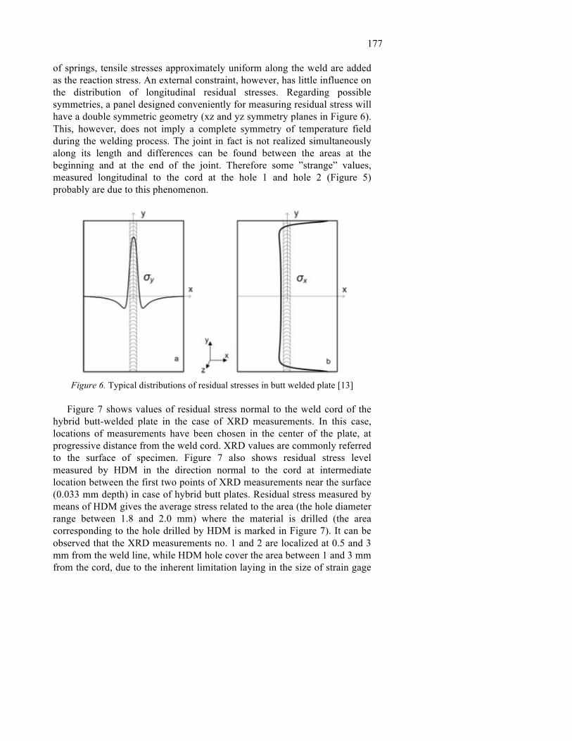
177 of springs, tensile stresses approximately uniform along the weld are added as the reaction stress. An external constraint, however, has little influence on the distribution of longitudinal residual stresses. Regarding possible symmetries, a panel designed conveniently for measuring residual stress will have a double symmetric geometry (xz and yz symmetry planes in Figure 6). This, however, does not imply a complete symmetry of temperature field during the welding process. The joint in fact is not realized simultaneously along its length and differences can be found between the areas at the beginning and at the end of the joint. Therefore some ”strange” values, measured longitudinal to the cord at the hole 1 and hole 2 (Figure 5) probably are due to this phenomenon.

Figure 6. Typical distributions of residual stresses in butt welded plate [13]

Figure 7 shows values of residual stress normal to the weld cord of the

hybrid butt-welded plate in the case of XRD measurements. In this case, locations of measurements have been chosen in the center of the plate, at progressive distance from the weld cord. XRD values are commonly referred to the surface of specimen. Figure 7 also shows residual stress level measured by HDM in the direction normal to the cord at intermediate location between the first two points of XRD measurements near the surface (0.033 mm depth) in case of hybrid butt plates. Residual stress measured by means of HDM gives the average stress related to the area (the hole diameter range between 1.8 and 2.0 mm) where the material is drilled (the area corresponding to the hole drilled by HDM is marked in Figure 7). It can be observed that the XRD measurements no. 1 and 2 are localized at 0.5 and 3 mm from the weld line, while HDM hole cover the area between 1 and 3 mm from the cord, due to the inherent limitation laying in the size of strain gage

C. Casavola, C. Pappalettere, F. Tattoli, F. Tursi rosette. Residual stress levels given by HDM (about 60 MPa corresponding to 0.033 mm depth) seem to be an intermediate value.

Figure 7. Calculated residual stresses normal to the cord on hybrid butt welded plate

by XRD

The results of the experimental fatigue tests are reported in table 6.

Table 6: Experimental results.

Specimen Nominal Stress Amplitude σa

[N/mm2]

Local Strain Amplitude εa

[µε]

Cycles to Failure

N

Final Crack Location

A1 80.6 700 151390 Weld cord A2 85.6 800 142497 Weld cord A3 60.5 512 589342 Weld cord A4 50.4 487 2181159 Weld defect A5 55.0 519 1533205 Weld defect A6 52.5 539 1313911 Weld defect

It should be noted that the fatigue failure occurs within the weld cord, or

near weld defects such as drops of fused material when they are presents. Similar results have been obtained in previous works [10, 11, 24] and they confirm the susceptibility of titanium to this kind of defects.

The fatigue strength of titanium grade 5 welded joints is also strictly dependent to the joining process parameters. Figures 8 and 9 show the fatigue curves, for a load ratio of 0.1, expressed in terms of nominal amplitude of stress σa and local amplitude of strain εa, according to the Wel.Fa.Re. method, of two different series of welded joints, welded both by hybrid technique, but with different parameters. “A” series has been studied in this work, “B” and “C” series are reported in a previous work [10].

179 Experimental data are fitted with a power law of Basquin’s type where the number of cycles to failure increases as a negative power function of stress range σa and of the local amplitude of strain εa.

Figure 8.Fatigue curve σa – N.

Figure 9.Fatigue curve εa - N.

It can be noted that “A” series has lower fatigue strength compared to “B”

and “C” series, and this result is due to different set of parameter in the joining process. The fatigue resistance for “A” series butt joints is lower of about 28% in terms of nominal amplitude of stress and of about 35% in terms of local amplitude of strain.

Figure 10 shows some the fatigue final fracture paths that are localized within the weld cord (butt A2, butt A3) and near drops of fused metal (butt A4). Crack initiation is highly affected by these defects and fatigues cracks initiate always from these sites if they are present.


Butt A2 Butt A3 Butt A4

Figure 10. Different fatigue fracture locations for hybrid butt titanium grade 5 welded joints.

In spite of the presence of these welding defects, fatigue curves expressed

in terms of both nominal amplitude of stress and in terms of local amplitude of strain are well correlated. It should be noted that for the “A” series the correlation factor is higher for the nominal amplitude of stress fatigue curve and this result is different for “B” and “C” series. The different grid length of strain gages used could cause it. In fact, in this work, 1.5 mm grid length has been used in order to measure the strain near the weld toe instead of 3 mm grid length used for “B” and “C” series. The strains are measured in a smaller area more closely to the weld cord. However the fatigue failures didn’t occur always within the weld cord or at the weld toe and a shorter grid length integrates the strains in smaller area in order to capture the local effect near the weld toe. For this reason, in this case, the local amplitude of strain can describe the fatigue behaviour of titanium grade 5 welded joints only in a partial way.

The analysis on the cross section of the fatigue failure surfaces by using a scanning electron microscope (SEM) has been carried out using a ZEISS evo microscope. Fractographic observations have been performed using the SEM operating in the secondary electron mode. In particular, the spacing of the fatigue striations on the fracture surfaces have been observed on surfaces perpendicular to the incoming electron beam. These observations were intended to give an indication of the local fatigue crack initiations and propagation during the test. Specimens have been cut and prepared in order to obtain the sample suitable for this kind of analysis. The effect of drops of fused metal distant from the weld cord has been investigated observing the cross section of the final fatigue fracture initiate from this site.

Figure 11 shows some fractographic observations on the fatigue fracture surface for the specimen Butt A2.

181

Figure 11. SEM observations of fatigue fracture surface for Butt A2 specimen.

In this case, the fatigue failure occurs within the weld cord, and it can be

noted the presence of porosity within the fused zone (Figure 11c). However the main crack responsible for fatigue failure is not localized near the porosities, but in the lower part of the specimen (Figure 11d). Figure 11a shows the fatigue striations and Figure 11b is the observation of zone with the static failure. The initiation of the main fatigue crack, can be noticed in Figure 11d. This result indicates that fatigue cracks can initiate in correspondence of weld defects, but the final failure can depend on other causes such as the local geometry of the weld cord and sharp notch present on the cord surface can influence more the fatigue strength of titanium grade 5 butt welded joints.

Figure 12 shows some fractographic observations on the fatigue fracture surface for the specimen Butt A4.

a) b)

c) d)


Figure 12. SEM observations of fatigue fracture surface for Butt A4 specimen.

In this case, the fatigue failure occurs near the drop of fused metal (Figure

12a), from this site it can be noticed the main fatigue crack. Figures 12b and 12c show the fatigue striations in different zones of the cross section, and Figure 11d shows a global observation obtained by the SEM microscope of the fracture surface. The fatigue crack growth rate is lower in Figure 12b and 12c, compared to Figure 12a. The higher crack propagation rate noticed in Figure 12a can be attributed to the presence of the fused metal drop that increases the stress concentration.

5. CONCLUSION

Hybrid (laser/MIG) butt welded joints have been considered in this work. Residual stress measurements have been executed by means of X-ray diffractometer, which gives a concentrated localized value of stress. Measured points are located along a direction transversal to the cord. Analysis of residual stresses measured values suggests the following considerations:

• HDM measurements on hybrid butt welded plate show that tensile stresses are produced in the transversal and longitudinal directions with respect to the weld cord and that longitudinal residual stress are higher than transversal residual stresses. These characteristics agree well with the results reported in the literature. • Regarding possible symmetries, a panel designed conveniently for measuring residual stress will have a double symmetric geometry. This, however, does not imply a complete symmetry of temperature

a) b)

c) d)

183

field during the welding process. The joint in fact is not realized simultaneously along its length and differences residual stress can be found between the areas at the beginning and at the end of the joint. • Tensile stresses in the transversal directions with respect to the weld cord near the cord become compressive distant from the weld cord. • Stress level measured near the surface in the direction normal to the cord by XRD on hybrid butt plate are in good agreement with the stress level relived by HDM measurements.

The fatigue behaviour of butt hybrid welded joints in titanium grade 5 has

been studied. σa – N and εa – N fatigue curves have been obtained. εa – N fatigue curve has been plotted according to the Wel.Fa.Re. method recommendations: two electric strain gauges have been bonded with their principal axes at 1 mm from the weld toe for each weld cord, then the local amplitude of strain is calculated applying the maximum and the minimum load of the fatigue test.

The local strain amplitude can account for the effects of many factors influencing fatigue life of welded joints and that the nominal stress concept could not appreciate. However in this case, the fatigue failures didn’t occur always within the weld cord or at the weld toe and the local amplitude of strain can describe the fatigue behaviour of titanium grade 5 welded joints only in a partial way.

Finally a comparison with the fatigue resistance of Ti6Al4V butt hybrid welded joints from a previous work has been presented. The fatigue resistance of titanium hybrid welded joints is strictly dependent to joining process parameters.

REFERENCES

1. ASM International. ASM Handbook Properties and Selection: Nonferrous Alloys and Special – Purpose Materials, vol. 2. 1992.

2. ASTM B265, Standard Specification for Titanium and Titanium Alloy Strip, Sheet and Plate. 2006.

3. Noolua NJ, Kerra HW, Zhoua Y and Xieb J. Laser weldability of Pt and Ti alloys. Materials Science and Engineering A, 397:8-15, 2005.

4. M. Ya, P. Marquette, F. Belahcene, J. Lu, Residual stresses in laser welded aluminium plate by use of ultrasonic and optical methods, Materials Science and Engineering A – Elsevier, 382:257–264, 2004.

5. M. Eboo, W. M. Steen,J. Clarke. Arc-augmented laser welding. Proc. of 4th International conference on advances in welding processes, Harrogate, UK, 1978.


6. Bang Hee Seon, Bang Han Sur, Kim You Chul, Oh Ik Hyun. A study on mechanical and microstructure characteristics of the STS304L butt joints using hybrid CO2 laser-gas metal arc welding. Materials and Design - Elsevier, 32:2328–2333, 2011.

7. F. Kong, R. Kovacevic. 3D finite element modeling of the thermally induced residual stress in the hybrid laser/arc welding of lap joint. Journal of Materials Processing Technology - Elsevier, 210:941–950, 2010.

8. G. A. Webster, A. N. Ezeilo. Residual stress distributions and their influence on fatigue lifetimes. International Journal of Fatigue - Elsevier, 23:S375–S383, 2001.

9. Structural Welding Code – Titanium. AWS D 1.9/D 1.9/M, 2007. 10. Casavola C, Pappalettere C and Tattoli F, Fatigue behaviour of hybrid

Ti6Al4V cruciform welded joints. Proceedings of New Trends in Fatigue and Fracture, Polignano a mare – Bari (Italy), July 2011.

11. Casavola C, Pappalettere C and Tattoli F, Confronto sulla resistenza a fatica di diversi tipi di giunti saldati in lega di titanio. Proceedings of IGF – Gruppo Italiano Frattura, Forni di Sopra – Udine (Italy), 1-3 March 2012.

12. C. Casavola, C. Pappalettere and F. Tattoli. Experimental and numerical study of static and fatigue properties of titanium alloy welded joints. Mechanics of Materials, 41:231-243, 2009.

13. G. Ivetic, A. Lanciotti, C. Polese. Electric strain gauge measurement of residual stress in welded panels. Journal of Strain Analysis, 44:117–126, 2009.

14. Stresstech group, X-ray Diffraction. The method for residual stress testing, 2003.

15. C. Casavola, R. Nobile and C. Pappalettere. Fatigue strength by the wel.fa.re. Local Strain Method: application to 3-5 mm cruciform and butt welded joints. SEM Annual Conference and Exposition on Experimental and Applied Mechanics, June 10-12 2002, Milwaukee (USA). 2002.

16. C. Casavola, R. Nobile and C. Pappalettere. Fatigue life predictions by the wel.fa.re. method: influence of residual stresses. SEM Annual Conference and Exposition on Experimental and Applied Mechanics, 2-4 June 2003, Charlotte (USA). 2003.

17. C. Casavola, R. Nobile and C. Pappalettere. A local strain method for the evaluation of welded joints fatigue resistance: the case of thin main – plates thickness. Fatigue & Fracture of Engineering Materials & Structures, 28:759-767, 2005.

18. C. Casavola and C. Pappalettere. Industrial application of a new local strain method for fatigue strength evaluation of welded structures. ICEM 12 International Conference on Experimental Mechanics, August 2004, Bari (Italy). 2004.

185 residual stresses caused by welding. Residual stresses can have a significant influence on the fatigue lives of engineering components [8]. In particular, near surface tensile residual stresses tend to accelerate the initiation and growth phases of the fatigue process while compressive residual stresses close to a surface may prolong fatigue life. Significant advances have been made in recent years for obtaining accurate and reliable determinations of residual stress distributions.

Fatigue strength of welded joints is lower than base material because of microstructure modifications, misalignment, geometrical discontinuity of the cord, residual stresses and weld defects. In order to take into account all the variables affecting the fatigue strength, the fatigue design of welded components is done on the basis of experimental results, using fatigue curves available in codes [9].

The fatigue behavior of a α + β Ti6Al4V alloy butt welded by hybrid technique has been investigated in this paper. The experimental results have been compared with a previous study on similar welded joints, but obtained with different process parameters [10-11]. Fatigue fracture surface have been observed by scanning electron microscope. Besides in this paper experimental hole drilling method and X-ray diffraction measurements have been reported.

2. MATERIAL AND METHODS

The material used in the tests was titanium grade 5 (Ti6Al4V), an α−β alloy with aluminium that is an α-stabilizing element and vanadium that is a β-stabilizing element. Ti6Al4V has good mechanical properties both at room and high temperature. Its density is half steel density (4.4 kg/dm3 [2]), the ultimate strength is 980 MPa and the yield strength is 760 MPa. Titanium grade 5 mechanical properties and chemical composition are indicated in tables 1 and 2.

Table 1: Mechanical properties of grade 5 titanium alloy [12]

Yield strength (MPa)


Young’s Modulus (MPa)

Elongation at fracture (%)

760 980 110200 14

Table 2: Chemical composition of titanium grade 5 according to ASTM B265 [2]

Element C Al V Fe H N O % < 0.08 5,5– 6.75 3,5– 4.5 < 0.30 < 0.015 < 0.03 < 0.25 At room temperature, unalloyed titanium has a hexagonal close-packed

(hcp) crystal structure called α-phase. At 883 °C this transforms to a body-

1

INFLUENCE OF GEOMETRIC SHAPE OF SPECIMEN IN FATIGUE LIFE CHARACTERIZATION ON WELDED JOINT IN TITANIUM ALLOY C. Casavola1, V. Giordano1, C. Pappalettere1, C. I. Pruncu1*

1Dipartimento di Ingegneria Meccanica e Gestionale, Politecnico di Bari, Viale Japigia, 182 - 70126 Bari, Italy Email address: [email protected]

Abstract: From literature we can find many theories on description of behaviour of different kind of materials. But just a few of them take into account an exact correlation between theoretical and experimental applications. In many instances the behaviour of these materials could be represented in function of some characteristics as density, Young modulus and Poisson ratio. One material with good characteristics of these listed above, that has been subjected to examination in this study, could be represented by titanium alloy and in particular titanium alloy grade 5. This material is suitable for the majority of applications in aeronautical, aerospace and naval industries and biomedical area. To be used in the field mentioned above, often titanium must be incorporated in different structures that can be obtained with welding process assembly. This new component could be more sensitive to crack initiation near the welded area due to the influence of the welding process. In this paper we try to elucidate some problems related to the fatigue life resistance of components simulating the activity during the real life of an assembly. The results have been confirmed by fractography analysis of broken surfaces, with a Scanning Electron Microscopy (SEM) and an optical microscope and have been correlated through numerical analysis.

Key words: FATIGUE LIFE, CRACK INITIATION, WELDED JOINTS

C. Casavola, C. Pappalettere, V. Giordano, C. I. Pruncu 1. INTRODUCTION

Material inhomogeneities are, in general, defects in the translational invariance of material properties. In a specimen different material regions can be seen, with rapid changes of microstructure and properties, which may be more or less smooth or even abrupt (1). Obviously it is virtually impossible to manufacture particles with perfectly smooth geometries (2).

The presence of micro defects in material due to certain variation of temperature or void merge during the process of fabrication is inevitable. The study of the physical process about the behavior of material can be dedicated to the nucleation phase of crack or void described with the inequality (a < am) (3), where am is the smallest crack length detectable by current technology, which is about 0.1µm. Heterogeneities in order of few micrometer are present in stainless steel as sulfide inclusions with size of 10 µm (4). In effect damage tolerance analysis which describes fatigue crack growth should be one connection to solve the fatigue nucleation stage.

In a theoretical vision, defects correspond to mathematical singularities in a continuous description that can be easily detected in the elastic field. An important subject of contemporary theoretical and applied mechanics is the fracture. The most relevant notions developed by engineers in that context are those of driving force acting on the tip of a crack and of energy-release rate.

2. OVERVIEW OF THE STATE OF THE ART

Description of fatigue initiation life in different medium, represented by solid mechanics and fluid mechanics fields, is yet open for all research society. Moreover, the technical society until today have provided in literature particular descriptions, lemmas and corollaries in goal to explain that topic. In next few lines, we will point some of the most important issue.

2.1 DEFINITION OF FATIGUE LIFE INITIATION

In literature, fatigue initiation life of solid materials, is assumed to be represented by the phase of crack initiation activity. In this way, for the description of this phase of crack initiation different definitions have been proposed. In absence of standard agreement, it is admitted to define the fatigue life initiation by a threshold crack length. The definition of the micro-crack initiation length is supposed to be quite equal to 0.1 mm for the majority of steels. This dimension is generally easy to detect and corresponds to a defect comparable to the steel grain size average. Fatigue initiation life is a consequence of cyclic slip in slip bands which implies

cyclic plastic deformation as result of moving dislocations. This micro-plasticity can occur more easily in the grains at the material surface. Accordingly the initiation fatigue life is supposed to be completed when micro-crack growth is no longer depending on the free surface conditions.

2.2 FATIGUE LIFE WITHOUT INITIATION

Some authors like Murakami (5) considered that each material contains a defect as a crack. Where the size is characterized by the root square of the ‘area’ parameter (‘area’ of the defect projected on the plane perpendicular to the direction of the maximum principal stress) and defined that crack initiation stage is negligible (Ni ≈ 0). Fatigue life is therefore assumed to be controlled by the crack propagation law.

2.3 FATIGUE INITIATION PARAMETER

In any case, fatigue resistance to initiation could be represented by a power relationship of the form Pi= f (Nib) where Pi is an initiation parameter and b exponent of Basquin’s type. Several approaches have been used to define the initiation parameter Pi: effective stress, notch stress intensity factor, damage parameter issued from SWT parameter (6), energy parameter.

It is acceptable to use stress range as a parameter to express fatigue resistance to initiation. In this case it is necessary to take into account that fatigue generally initiates from stress concentration area which induce stress gradient at notch tip. Stress distribution at notch tip was assumed to derive from Irwin’s elastic stress distribution at crack tip by Creager and Paris (7). To avoid stress singularity at notch tip the Irwin stress distribution at notch tip is shifted by introduction of a new origin located at distance ρ/2 to the previous one. The stress distribution is governed by the (crack) stress intensity factor K and represented by :

3cos 1 sin sin2 2 2 2 22 2

I Iyy

K Krr r

θ θ θ ρ θσ

π π⎡ ⎤= + +⎢ ⎥⎣ ⎦ (1)

where r and θ are polar coordinates and ρ the notch radius This method assumed that the effective stress is the maximum stress

located at notch tip which is given by:

( ) 22, 0max

Kxyy ρ θσ σπρ

= = = = (2)

C. Casavola, C. Pappalettere, V. Giordano, C. I. Pruncu

Barsom and McNicol (8), Jack and Price (9), Clark (10) and Truchon (11)

have used the parameter K ρΔ to express fatigue resistance on notched specimens.

This fatigue resistance can be expressed by the concept of effective stress range (12) Δσef which represents the average stress over the fatigue process volume often reduced to the average stress over the effective distance Xef due to the assumption that this volume is cylindrical.

0

1 ( )ef

ef yyef

Xr dr

Xσ σ=Δ Δ∫ (3)

Lukas et al. (13) approximated this stress by an equivalent stress in

proximity of a notch tip prolongated with fictitious microcracks by the following relationship:

,

01 4.5t g

eq Lukas

ka ρ

σσ

ΔΔ =

+ (4)

kt is the elastic stress concentration factor σg the applied gross stress

range. The fictitious microcrack length used by Lukas et al (14) is here assumed equal to ao:

( )

21

0K thaDπ σ

Δ= (5)

where σD is the fatigue limit and ΔKth the fatigue threshold. Due to stress concentration, cyclic plasticity occurs generally at notch tip

and elasto-plastic stress distribution is generally more complex than the elastic one and it can be obtained by Finite Element computing. By applying effective stress range definition given in formula (3), Capelle and al (15) have presented fatigue resistance to initiation of an X52 pipe steel.

The stress distribution at notch tip at a distance greater than the effective distance can be described by the so-called Notch Stress Intensity Factor (NSIF). Lazzarin et al (16) use the elastic NSIF K* as parameter for fatigue initiation. Boukharouba et al (17) have compared fatigue initiation criteria with a criterion based on the elasto-plastic notch stress intensity factor Kρ on welded specimens made in low strength steel; The weld toe was considered as a notch with a notch angle of 135°. The NSIF has then unit MPa *mα

191 where α is the power dependence of the stress distribution (α = 0.385).

Smith et al (18) have shown experimentally that the result of equation (6)

is constant whatever the stress ratio is:

.max C SWTE aσ ε = = (6) where σmax is the maximum stress, E the Young’s modulus and εa the

strain amplitude. This result is called the SWT parameter and it is generally used to convert low cycle fatigue resistance at zero stress ratio to low cycle fatigue resistance at any stress ratio. Lazzarin et al (16) have derived a so-called damage parameter D from the SWT parameter and expressed it as a stress (MPa*units); They have presented that for thin plates notched by symmetric lateral U-, V- shaped notches with notch root radii ranging from 0.1 to 10 mm and made in steel. All the results merge in a unique curve independently of the notch radius.

Fatigue crack initiation of engineering components exhibiting

significantly small dimensions imperfections ‘‘short flaws’’ is expressed as :

0th

c

KF a

σπ

ΔΔ =

(7) where F is a geometrical factor. This fatigue initiation stress range for both short and long crack is

expressed by Kitagawa and Takahashi diagramme (19) where the crack growth threshold is plotted against the crack size.Using empirical law relationship (5) we can write:

( )0

0

thc

KF a a

σπ

ΔΔ =

+ (8) Another formula is presented by Jelaska and Podrug (20) in cumulative

HCF/LCF loading:

0

2

i

i i

mgr

i m mU a m

U a m HCF

NN

n

σ

σ σ σσ σ σ

=⎛ ⎞

+⎜ ⎟+ −⎝ ⎠ (9) where mi ,σu, σa, σm, σ0, Ngr, nHCF are material constant, ultimate strength,

violeta

Pencil

C. Casavola, C. Pappalettere, V. Giordano, C. I. Pruncu stress amplitude, maximum stress, endurance limit, sufficiently long fatigue life, number of HCF cycles.

3. MATERIALS AND WELDED BUTT JOINTS

In last period materials as titanium and titanium alloy are finding

widespread applications due their good characteristics. Consequently they show a good balance of mechanical and chemical properties and hence cover many areas of application in diverse industries. The most widely used titanium alloy is Ti-6Al-4V ( α–β alloys ). These alloys contain larger amounts of beta stabilizers (4 to 6%) (21). Compared with steel, titanium or titanium alloys have low density and shows a similar fatigue resistance and presents a very attractive strength weight ratio.

The most influential microstructural parameter on the mechanical properties of titanium alloys can be influenced by either a alloys (hexagonal crystal structure) or β alloys (body centered cubic structure) and a–b alloys. Properties of α–β alloys (titanium grade 5) can be controlled through heat treatments (22), (23). Chemical compositions of tested materials are reported in Table 1 and Table 2.

Table 1. Chemical composition of titanium alloy grade 5.

Titanium grade 5

C Al V Fe H N O

ASTM B265

<0.08 5.5-.75 3.5-4.5 <0.30 <0.015 <0.03 <0.25

Table 2. Mechanical properties of titanium alloy grade 5.

Titanium grade 5

Modulus of elasticity E [MPa]

Ultimate tensile strength R [MPa]

Yield tensile strength R02

[MPa] ASTM B265

1.138 956.4 760

The alloy is recommended mainly for design disks, blades, spacer rings, engine body and other aircraft-engine, components operating at temperatures up to 400–450°C (24). In the case where these materials are integrated in structure mentioned above, different procedures for joining are used. One possibility is to use mechanical joining by welding process as butt welded joint. Cited by Casavola et al (22), specimens obtained by process of

193 welding and more precisely “butt welded joint” show sensitivity to fatigue life initiation at conjunction of weld cord and parent material. Of course, in this region, which corresponds to the heat affected zone (hosting microstructural changes) the stress/strain field is usually amplified with respect to the nominal stress values because of the effects of local geometry of the seam, localized plasticization and secondary bending produced by misalignments.

In the other hand, one great problem is represented by the slags which are formed and deposited, during the welding process, in proximity of the weld cord. Due to the difficult task to eliminate these entities caused by solidification, life of butt welded joint could decrease. For example using metal removal in steels and low alloy steels, can cause un-tempered martensitic to form, which is brittle and causes significant shortening of fatigue life. In this case the welding processes must be improved, redefining welding time and speed (25). Figure 1 shows the approximate profiles recognized by a tactile device, acquired namely by a Coordinate Measuring Machine (CMM) for the right and reverse sides of the butt welded specimen.

Figure 1. Butt welded joint specimen: right (upper) (a) and reverse (lower) (b) side seam profile.


After fatigue tests, on specimens of butt welded joint of titanium alloy,

a summary of macrographies about details of microstructure has been

C. Casavola, C. Pappalettere, V. Giordano, C. I. Pruncu illustrated. Thus such macrography, characterizes areas where initiation of crack occurs. In this way are taken samples all over the material surface, both from the welding area connection and also from the area where the slags irregularities are deposited. With an optical microscope we show the arrangement of grains, in which we can see the distribution of lamellar grains. In figure 2 we can see the distribution of microcracks between grains which occur concerning intergranular life initiation.

Figure 2. Microcrack initiation in intergranular mode, titanium alloy Ti-6Al-4V (α−β)

On the other hand, in the adjacent area of slag we found some inclusions which can lead to trigger the process of fatigue. Difference in color between material layer under the slag and titanium alloy displayed in figure 3 (a), leads to the idea that, in this area could be occurred a chemical process in different way that also influences the fatigue behavior. At the interface of these layers in figure 3 (b), is evident the distribution of line of fatigue.

Site of life initiation fatigue

195 Figure 3. Site of fatigue initiation characterized through a) inclusion on the slag area, b) line of life initiation fatigue

Under some influences of temperature variations, correlated with the

fatigue damage test effect involved, the critical strain in ductile mode fracture is locally showed. Exceeded this critical strain shear bands and small voids are formed. These voids are known as strain induced porosity (SIP). An example of strain induced porosity in Ti-6Al-4V is shown in figure 4. Once this porosity is created in forging billet, it is not always healed during subsequent forging operations. Consequently, it can be carried over into a finished component as a defect that can act as an early fatigue crack initiation site (25).

Figure 4: Representation of face of crack initiation life In order to correlate the experimental results, we apply the numerical

analysis model. Models with Extended Finite Element Method (XFEM) have been realized and the analysis has been executed through Abaqus Software. The numerical model considered had the same shape of butt welded joint acquired by the Coordinate Measuring Machines. For fatigue tests a value of charge loading of 24.5 kN has been imposed. According with the experimental results, the model has incorporated one irregularity. This irregularity is exemplified through one crack of about 0.1 mm in the weld cord area. Shape of specimen is represented in figure 4 a). Although, this crack may produce implications, expecting an increase of stress in the welded cord area, an obvious increase in stress in the slag area, has been registered. These trends of stress distribution are showed in figure 5 b). This complex behaviour can be explained by the appearance of inclusions under the slag area as displayed in figure 6.


Figure 5: a) Shape of specimen analyzed with crack in weld area, b) Distribution of maximal stress versus displacement in the sample with and without inclusion

Figure 6: Model of butt welded joint with inclusion in the slag area

5. CONCLUSION

Experimental determination and numerical analysis of fatigue life initiation are illustrated in this paper. Thus, factors which could influence the behavior of butt welded joint specimen are determined. Some specific parameters which could be mentioned are : distribution of boundary grains on material which show lamellar form and early phase in microcrack intergranular behavior, varieties of some inclusion unexpected in base

a) b)

197 material, difference of temperature in the bonding area represented through interface slag and parent material. The same could be cited about factors regarding the growing in size of voids, which involve the strain behavior and initiation life.

On the other hand, by XFEM is presented the distribution of stress along the shape of butt welded joint and the behavior of one irregularity in the body of material alloy, through which we can deduce that, the true life initiation of fatigue, in titanium alloy, is represented by a complex of parameters from shape of material to manufacturing process.

REFERENCES

1.Arkadi Berezovski. Numerical Simulation Of Waves And Fronts In Inhomogeneous Solids. World Scientific Publishing Co. Pte. Ltd., London,ISBN-13: 978-981-283-267-2, 2008.

2.T.I. Zohdi. Introduction to Computational Micromechanics,. Society for Industrial and Applied Mathematics, ISBN 978-0-898716-27-6, 2007.

3.J.K. Paik. Conditionassessment assessment of aged structures. s.l. : Woodhead Publishing Limited, ISBN 978-1-84569-334-3, 2008.

4.E. McCafferty. Introduction to Corrosion Science. s.l. : Springer Science+Business Media, LLC., New York, ISBN 978-1-4419-0454-6, 2010.

5.Y. Murakami, S. Kodamab and S. Konumac. “Quantitative evaluation of effects of non-metallic inclusions on fatigue next term strength of high strength steels”. International Journal of Fatigue, Volume 11, Issue 5, Pages 291-298, September 1989.

6.K. N. Smith, P.Watson and T. H.Topper. A stress-strain function for the fatigue of metals,. Journal of Materials, JMLSA, 5, 767-778, 1970.

7.M. Creager and P. C. Paris. Elastic field equations for blunt cracks with reference to stress corrosion cracking,. Int.J. Fracture Mech. 3, 247-252, 1967.

8.M. Barsom and R. C. McNicol. Effect of stress concentration on fatigue-crack initiation in HY-130 steel,. ASTM STP 559, 183-204 , 1974.

9.A. R. Jack and A. T. Price. The initiation of fatigue cracks from notches in mild steel plates,. Int. J. Fracture Mech. 6 (4) ,1970.


10.W. G. Clark, Jr. Evolution of the crack initiation properties of type 403 stainless steel in air and steam environment,. ASTM STP 559, 205-224,1974.

11.M. Truchon. Amorçage de fissures en fatigue à partir d'entaille, application aux joints soudés,. Bulletin Technique du Bureau Veritas 67 (5),1985.

12.G. Pluvinage. Fatigue and Fracture emanating from stress concentrators,. Kluwer,Dordrecht, ISBN: 1-4020-2612-9, 2003.

13.P. Lukas, L. Kunz, B. Weiss, and R.Stickler. Non-damaging notches in fatigue. Fatigue & Fracture of Engineering Materials & Structures, 9, 195-204, 1986.

14.P. Lukas. Stress intensity factor for small notch-emanating cracks,. Eng. Fract Mech., 26:471–3, 1987.

15.J. Capelle, J. Gilgert, G. Pluvinage. A fatigue initiation parameter for gas pipe steel submitted to hydrogen absorption,. International Journal of Hydrogen Energy, Volume 35, Issue 2, January, Pages 833-843, 2010.

16.P. Lazzarin, R. Tovo and G. Meneghetti. Fatigue crack initiation and propagation phases near notches in metals with low notch sensitivity,. Int. J. Fatigue Vol. 19, Nos 8-9, pp. 647-657, 1997.

17.T. Boukharouba, T. Tamine,L. Niu, C. Chehimi and G. Pluvinage. The use of notch stress intensity factor as a fatigue crack initiation parameter,. Engineering Fracture Mechanics, Vol. 52, No. 3, pp. 503-512, 1995.

18.R.A. Smith, K.J. Miller. Prediction of fatigue regimes in notched components,. Int J Mech Sci., 20:201–6, 1978.

19.H. Kitagawa, S. Takahashi. Applicability of fracture mechanics to very small cracks or cracks in the early stage. In: Proceedings of second international conference on mechanical behaviour of materials,. ASM., p. 627–31,1976.

20.D. Jelaska, & S. Podrug. Crack initiation limits prediction at combined HCF/LCF loading,. Advanced Engineering, ISSN 1846-5900, 2, 2008.

21.Vydehi Arun Joshi. Titanium Alloys An Atlas of Structures and Fracture Features. Taylor & Francis Group, ISBN 0-8493-5010-7 , LLC, Boca Raton, 2006.

22.C. Casavola, C. Pappalettere, F. Tattoli. Experimental and numerical study of static and fatigue properties of titanium alloy welded joints. Mechanics of Materials 41, 231–243 , 2009.

199

23.ASM International. ASM Handbook Properties and Selection:

Nonferrous Alloys and Special – Purpose Materials. vol. 2,1992. 24.Valentin N.Moiseyev. Titanium Alloys Russian Aircraft and

Aerospace Applications,. Taylor & Francis Group 6000 Broken Sound Parkway NW, Suite 300, ISBN 0-8493-3273-7,2006.

25.Gerd Lütjering, James C. Williams. Titannium,. Springer-Verlag Berlin Heidelberg, ISSN 1619-0181, 2007.

Documents

NT2F12