Mannheimer Manuskripte zu Risikotheorie, Portfolio Management und Versicherungswirtschaft

Nr. 171

A Data-Analytic Examination

of the Risk in Hedge Funds Returns:

The g-and-h Distribution

von JOCHEN MANDL

Mannheim 09/2007

A Data-Analytic Examination of the Risk in Hedge Funds Returns: The g-

and-h Distribution

Introduction

In the recent years the alternative asset class of hedge funds is widely discussed in financial

literature. On the one hand this is caused by an increasing demand on these unregulated in-

vestments1 and on the other hand it is caused by a lack of transparency concerning their in-

vestment strategies and investment instruments used. Especially this lack of knowledge gives

reason to an unreflected adaption of the standard arguments of the attractiveness of a hegde

fund investment, for example like a high expected return is going together with a low to a

moderate risk.2 Therefore this lack of knowledge gives reason to hope for a lasting substantial

improvement of the return/risk-profile through the incorporation of such an investment.

In exploring hedge fund return patterns there are a variety of problems concerning the quality

of the data and their structural behaviour. Regarding the quality of the data one can for exam-

ple distinguish well documented biases, as the self-selection bias, the survivorship bias, the

backfill bias and the liquidity bias.3 In attaining satisfactory results concerning the quality of

the data the following analysis is based on a subset of hedge fund index data chosen from the

established data vendor Credit Suisse/Tremont from January 1994 till June 2005.4

Summarizing the problems concerning the structure of the data one can first mention the com-

paratively small amount of return data. Moreover numerous empirical studies lead to a sub-

stantial body of evidence that hedge fund return data rarely exhibit the ideal behaviour postu-

lated by the Gaussian distribution.5 Generally such results are obtained by using the following

procedure: First of all the hypothesis of normality is rejected qualitatively by arguments con-

cerning special style characteristics of a hedge fund investment. In a second step this qualita-

tive result is affirmed empirically based on quantitative methods. To sum up the studies men-

1 See Eling 2006, p. 19 et sqq. 2 See the empirical results supporting the above argumentation for a specified time-frame in Liang 1999 and Kazemi/Schneeweis 2004, p. 5. 3 See Lhabitant 2004, pp. 88-95, Bessler/Drobetz/Henn 2005, p. 24 et sqq. 4 The selection of this database was mainly driven by its size, by the asset weighted index construction and the effort of mitigate biases like the survivorship bias. A detailed overview of existing databases can be found in Lhabitant 2004, p. 88 and Bessler/Drobetz/Henn 2005, p. 22. 5 Regarding the above mentioned index data Eling 2006, Appendix C. Regarding individual hedge funds see the empirical results in Agarwal/Naik 2000a, Agarwal/Naik 2000b; Fung/Hsieh 1997 and Fung/Hsieh 1999. A de-tailed overview can be found in Liang/Park 2007.

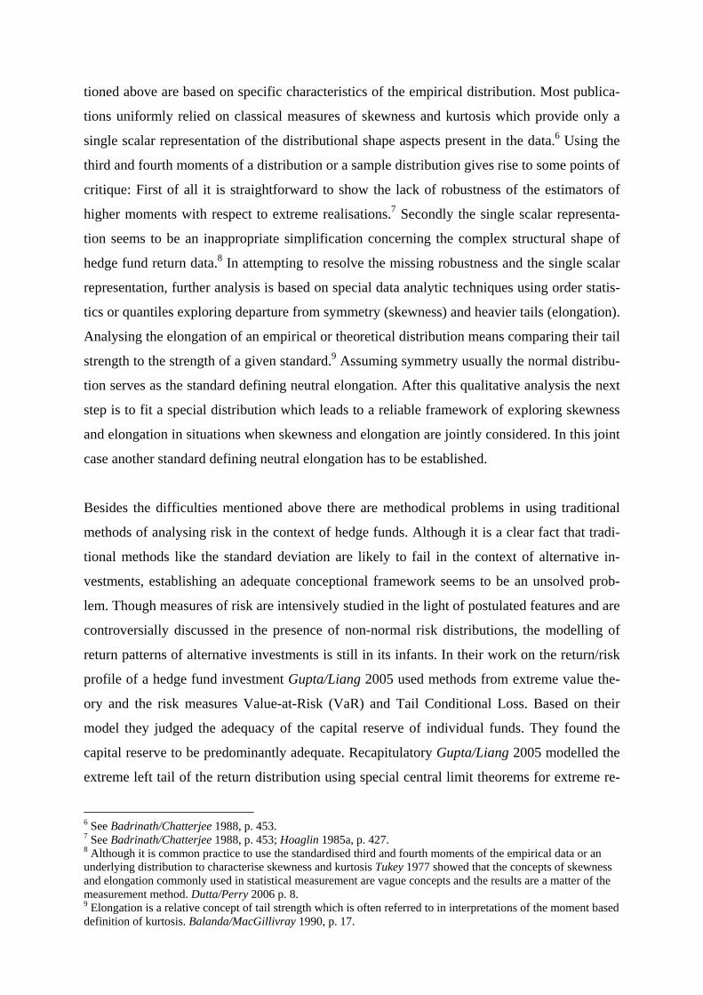
tioned above are based on specific characteristics of the empirical distribution. Most publica-

tions uniformly relied on classical measures of skewness and kurtosis which provide only a

single scalar representation of the distributional shape aspects present in the data.6 Using the

third and fourth moments of a distribution or a sample distribution gives rise to some points of

critique: First of all it is straightforward to show the lack of robustness of the estimators of

higher moments with respect to extreme realisations.7 Secondly the single scalar representa-

tion seems to be an inappropriate simplification concerning the complex structural shape of

hedge fund return data.8 In attempting to resolve the missing robustness and the single scalar

representation, further analysis is based on special data analytic techniques using order statis-

tics or quantiles exploring departure from symmetry (skewness) and heavier tails (elongation).

Analysing the elongation of an empirical or theoretical distribution means comparing their tail

strength to the strength of a given standard.9 Assuming symmetry usually the normal distribu-

tion serves as the standard defining neutral elongation. After this qualitative analysis the next

step is to fit a special distribution which leads to a reliable framework of exploring skewness

and elongation in situations when skewness and elongation are jointly considered. In this joint

case another standard defining neutral elongation has to be established.

Besides the difficulties mentioned above there are methodical problems in using traditional

methods of analysing risk in the context of hedge funds. Although it is a clear fact that tradi-

tional methods like the standard deviation are likely to fail in the context of alternative in-

vestments, establishing an adequate conceptional framework seems to be an unsolved prob-

lem. Though measures of risk are intensively studied in the light of postulated features and are

controversially discussed in the presence of non-normal risk distributions, the modelling of

return patterns of alternative investments is still in its infants. In their work on the return/risk

profile of a hedge fund investment Gupta/Liang 2005 used methods from extreme value the-

ory and the risk measures Value-at-Risk (VaR) and Tail Conditional Loss. Based on their

model they judged the adequacy of the capital reserve of individual funds. They found the

capital reserve to be predominantly adequate. Recapitulatory Gupta/Liang 2005 modelled the

extreme left tail of the return distribution using special central limit theorems for extreme re-

6 See Badrinath/Chatterjee 1988, p. 453. 7 See Badrinath/Chatterjee 1988, p. 453; Hoaglin 1985a, p. 427. 8 Although it is common practice to use the standardised third and fourth moments of the empirical data or an underlying distribution to characterise skewness and kurtosis Tukey 1977 showed that the concepts of skewness and elongation commonly used in statistical measurement are vague concepts and the results are a matter of the measurement method. Dutta/Perry 2006 p. 8. 9 Elongation is a relative concept of tail strength which is often referred to in interpretations of the moment based definition of kurtosis. Balanda/MacGillivray 1990, p. 17.

alisations, which in general seems to be inappropriate in the case under consideration. Beyond

that critique special notice should be given to the results of Degen/Embrechts/Lambrigger

2006. They explore the characteristics of a special distribution model, the g-and-h distribu-

tion, which has received special attention in modelling operational risk, in the light of the ex-

treme value theory. They show that in situations in which the g-and-h model is an appropriate

description for the data at hand, the use of methods based on extreme value theory leads to

nonsatisfying results. Also Liang/Park 2007 explore diverse loss based risk measures. Their

application was based on parametric as well as on non parametric methods. The Cor-

nish/Fisher-Expansion played a special role in their analysis.

The present paper supports in a first step the result of non normal hedge fund returns based

upon robust exploratory data analytic techniques. In addition the g-and-h distribution pro-

posed by Tukey 1977 is fitted to the data. This approach exhibits a clear and straight structural

form, is easy to apply and moreover provides an excellent fit for the entire data set. In addi-

tion this parametric model offers a high flexibility in modelling the shape of the distribution.

For example the fitted distribution is allowed to have different structures in the two tails.10

But one has to be aware of the problems and consequences of over fitting the model. In gen-

eral the g-and-h distribution offers a genuine and flexible way of detailed exploration of

skewness and elongation which is somewhat superior to classical moment based measures.

The second contribution of this paper regarding existing hedge fund literature like

Gupta/Liang 2005 and Liang/Park 2007 is an enhancement of existing methods quantifying

risk in that it provides a new VaR-approach based on the g-and-h distribution.

Exploratory Data Analysis

CS/Tremont offers an aggregate hedge fund index based on 437 representative individual

funds as well as 13 indices representing individual hedge fund styles respectively strategies.

The styles can for example be divided into the three following groups: Market Neutral, Event

Driven and Opportunistic. An important criterion concerning a classification system of hedge

fund styles is their sensitivity to changes in the financial markets. Figure 1 summarises the

chosen classification system for chosen style indices in short.

10 See Badrinath//Chatterjee 1988, p. 454.

HEDGE FUNDS

Market Neutral Event Driven Opportunistic

Convertible Arbitrage

Fixed Income Arbitrage

Equity Market Neutral

Distressed Securities

Risk / Merger Arbitrage

Emerging Markets

Short Sellers

Long / Short Equity

Global Macro

SensitivityLow(non-directional)

High(directional)

figure 1

Prior to fitting the parametric model, a first analysis of skewness and elongation is based on

special data analytic techniques using selected quantiles. These techniques measure skewness

and elongation of the data with respect to the skewness and elongation of the Gaussian distri-

bution. A common approach in choosing these quantiles mentioned above is to use letter val-

ues first proposed by Tukey 1977 and incorporated in Hoaglin 1985a. In doing so one has to

choose the sequence of α-quantiles so that the probability α successivley always halves, i.e.

,...,16/1,8/1,4/1=α . For each α there is a corresponding pair of quantiles, the α-quantile

(lower quantile) and the (1−α)-quantile (upper quantile). As a consequence of successively

halving α the selected quantiles come more from the tails than from the body of the data.11

Therefore further analysis can be based on a set of quantiles instead of one special pair alone

to get a closer and more robust look at skewness and elongation. In doing so asymmetry and

heavy tails can be considered graphically as follows.

In a first step the skewness of the data is judged by the midsummary statistic. Intuitively, if

the situation at hand is symmetric, each corresponding pair of quantiles must be symmetri-

cally placed around the median, which is the point of symmetry. Following this intuition the

midsummary statistic for the data { }NiiX 1= is calculated as:

11 See Hoaglin 1985a, p. 419. The optimal spacing of the quantiles usually depends on the correlation structure of the order statistics. Typically less information in the form of quantiles is needed to model the body of the distribution than to model the tails of the distribution. Dutta/Perry 2006, p. 77.

)(5.0 )1( ααα −+= QQMid , (1)

in which αQ represents the above defined α-quantile of the data. The plot of the midsumma-

ries versus various levels of α can help judging whether there is a systematic pattern in the

data.12 If there is a regular or a moderately regular steady increase or decrease from one mid-

summary to the next one can talk about a systematic skewness.13 Summing up regular patterns

in the midsummaries reveal the presence of skewness and moreover their direction. Following

figure 2 illustrates the results concerning the CS-style indices.

CS-Composite

0,000

0,002

0,004

0,006

0,008

0,010

0,012

0,014

0,016

F E D C B A 1

Letter Value

Mid

sum

may

CS-Convertible Arbitrage

-0,008

-0,006

-0,004

-0,002

0,000

0,002

0,004

0,006

0,008

F E D C B A 1

Letter Value

Mid

sum

may

CS-Fixincome Arbitrage

-0,035

-0,025

-0,015

-0,005

0,005

0,015

0,025

F E D C B A 1

Letter Value

Mid

sum

may

CS-Equity Market Neutral

0,000

0,005

0,010

0,015

0,020

0,025

F E D C B A 1

Letter Value

Mid

sum

may

CS-Distressed Securities

-0,055

-0,045

-0,035

-0,025

-0,015

-0,005

0,005

0,015

0,025

F E D C B A 1

Letter Value

Mid

sum

may

CS-Riskarbitrage

-0,015

-0,010

-0,005

0,000

0,005

0,010

0,015

0,020

0,025

F E D C B A 1

Letter Value

Mid

sum

may

12 Brizzi 2003 explores the statistic „letter coefficient of skewness“ as a quantitative method of judging skew-ness. This statistic is also based on the above defined midsummaries using letter values. In spite of basically positive characteristics of the statistic one can find a lack of robustness in the presence of extreme realisations. As a consequence the letter value of skewness is not applied to the present data. 13 See Hoaglin 1985a, p. 425; Dutta/Perry 2006, p. 9.

CS-Dedicated Short

-0,010

0,000

0,010

0,020

0,030

0,040

0,050

0,060

0,070

0,080

F E D C B A 1

Letter Value

Mid

sum

may

CS-Emerging Markets

-0,045

-0,035

-0,025

-0,015

-0,005

0,005

0,015

0,025

F E D C B A 1

Letter Value

Mid

sum

may

CS-Global Macro

-0,010

-0,005

0,000

0,005

0,010

0,015

0,020

0,025

F E D C B A 1

Letter Value

Mid

sum

may

CS-Long/Short-Equity

0,000

0,005

0,010

0,015

0,020

0,025

F E D C B A 1

Letter Value

Mid

sum

may

figure 2

The Composite Index reveals only unsystematic variation of the midsummaries around the

median, which argues against a systematic skewness at least for the body of the data. Patterns

suggesting systematic left skewed data can be found for the Convertible Arbitrage, the Fixed

Income Arbitrage, the Distressed Securities and the Risk Arbitrage Index. The Dedicated

Short Index obviously exhibits a right skewed pattern. On the other hand the Equity Market

Neutral Index reveals midsummaries at the same level of the median and can hence be seen as

symmetric. The residual indices from the set of opportunistic strategies, the Emerging Mar-

kets, the Global Macro and the Long/Short Equity Index show similar patterns in the sense

that there are, but different, systematic patterns for the body and tail areas of the data. Sum-

ming up there is evidence for all indices, that symmetry cannot be rejected at least for the

body of the data. Therefore a normal approximation for the body of the data seems to be ap-

propriate.

Regarding the classification system in figure 1 the following statements can be made: The

Equity Market Index reveals to be symmetric and can be considered as the odd one out in the

set of Market Neutral Indices. The others show a systematic skewness to the left, whereas the

plot of midsummaries follows a regular pattern for all levels of α. The indices building up the

set of Event Driven strategy reveal a systematic skewness to the left as well, but display a

more complex structure of decrease. This manifests itself by means of a slight decrease of the

midsummaries for the more central quantiles under consideration and a notable stronger de-

crease of the midsummaries for the extreme quantiles. Just as the latter, the plot for the oppor-

tunistic, except for the Dedicated Short Index, follows a complex but similar pattern. All in all

these results under consideration, with the exceptions mentioned, support the used classifica-

tion.

In the following elongation is measured. For this purpose the pseudosigma statistic is de-

fined:14

PZ

XXPseudo2

1 ααα

−= − , (2)

whereas PZ is the α-quantile of the standard normal distribution. This measure relates the

positive distance of corresponding α-quantiles (upper and lower) to the standardnormal coun-

terpart. If there is a systematic increasing (decreasing) behaviour in the plot of the pseudosig-

mas versus different levels of α, this is indicative for positive (negative) elongation.15 Figure

3 illustrates the pseusosigmas of the stated indices:

CS-Composite

-3

2

7

12

17

22

27

F E D C B A 1

Letter Values

Pseu

dosi

gma

CS-Convertible Arbitrage

-3

2

7

12

17

22

27

F E D C B A 1

Letter Values

Pseu

dosi

gma

CS-Fixincome Arbitrage

-3

2

7

12

17

22

27

F E D C B A 1

Letter Values

Pse

udos

igm

a

CS-Equity Market Neutral

-3

2

7

12

17

22

27

F E D C B A 1

Letter Values

Pse

udos

igm

a

14 See Hoaglin 1985a, p. 426. 15 See Hoaglin 1985a, p. 427.

CS-Distressed Securities

-3

2

7

12

17

22

27

F E D C B A 1

Letter Values

Pseu

dosi

gma

CS-Riskarbitrage

-3

2

7

12

17

22

27

F E D C B A 1

Letter Values

Pseu

dosi

gma

CS-Dedicated Short

-3

2

7

12

17

22

27

F E D C B A 1

Letter Value

Mid

sum

may

CS-Emerging Markets

-3

2

7

12

17

22

27

F E D C B A 1

Letter Values

Pse

udos

igm

a

CS-Global Macro

-3

2

7

12

17

22

27

F E D C B A 1

Letter Values

Pse

udos

igm

a

CS-Long/Short Equity

-3

2

7

12

17

22

27

F E D C B A 1

Letter Values

Pse

udos

igm

a

figure 3

Figure 3 illustrates the systematic elongation inherent in the data. Indeed for all strategies

there is the same structural behaviour of the pseudosigmas though in a different magnitude.

The most noticeable patterns are those of the Dedicated Short Index and the Emerging Mar-

kets Index. As in the context of skewness the elongation of the Equity Market Neutral Index is

the fewest of all. However one thing has to be pointed out about the correct use of the peseu-

dosigma statistic. Usually judging elongation using pseudosigmas is based on the working

hypothesis of a symmetric distribution. For this very reason, having the midsummary patterns

in mind, elongation can be confounded with the effects of skewness and moreover a distinct

analysis of skewness-induced elongation and further elongation is not feasible.16 Summarising

fitting a model to the data at hand requires an approach flexible enough in describing the pre-

16 As in the symmetric case neutral elongation is defined by the normal distribution, but in the presence of skew-ness a new standard defining neutral elongation has to be established.

vailing patterns of skewness and elongation in situations in which they occur jointly in the

data.

The g-and-h distribution

The g-and-h distribution was first proposed by Tukey 1977 and is further analyzed by Hoaglin

1985b. This type of distribution is flexible enough to model a variety of different skewness

and elongation patterns.17 The ability of approximating a wide variety of distributions, com-

monly used in modelling financial data, only by means of a specific choice of a few parame-

ters is the advantage of the g-and h-distribution.18 The estimation of parameters can basically

be made on the basis of the maximum likelihood-method, the method-of-moments approach

or it can be based on quantiles.19 Robust methods have, as already explained, favourable char-

acteristics concerning the estimation of the tails, therefore they will be applied in the follow-

ing. Furthermore, the structural form of the transformation of a standard normal distributed

random variable is particularly suitable for a quantile-based estimation.20 For a more detailed

presentation of the quantile-based estimation of parameters see Hoaglin 1985b, Dutta/Perry

2006 and Mills 1995.

Currently the g-and-h distribution is being used successfully in order to quantify operational

risks in the context of banking and insurance.21 In addition, Mills 1995 and Badri-

nath/Chatterjee 1988 successfully modelled stock market returns using this distribution. Bab-

bel/Dutta 2002 model skewness and elongation of the LIBOR and in Babbel/Dutta 2005 the

g-and-h distribution serves as a starting point in option pricing.

Formally, the g-and-h distribution results from a non-linear transformation of a standard nor-

mal distributed random variable with real valued parameters a, b, g and h. In this case the pa-

17 In addition there are other distributions, which were proposed for modeling skewness and elongation. See Fischer/Horn/Klein 2003. They compare different distributions in the presence of skewness and positive elonga-tion and get compelling results using the g-and-h distribution. 18 See Martinez/Iglewicz 1984, p. 363 et sqq.; Dutta/Perry 2006, p. 14. 19 See MacGillivray/Rayner 2002a; MacGillivray/Rayner 2002b; Badrinath/Chatterjee 1988, p. 455. 20 See Dutta/Perry 2006, p. 17. 21 See Perry/Dutta 2006, Albrecht/Schwake/Winter 2007.

rameter a accounts for the location and b accounts for the scale.22 The skewness and elonga-

tion are controlled by the parameters g and h, what ensures the desired flexibility.23

Assuming that Z is a standard normal distributed random variable, X follows a g-and-h distri-

bution if X satisfies:24

g

eebaXhZ

gZ)2/( 2

)1( −+= (3)

From this relation two different distributions arise for 0=g or 0=h as special cases:25

gebaX

gZ )1( −+= the g-distribution in the first case and (4)

)2/( 2hZZbeaX += the h-distribution in the second case.26 (5)

At this point it is evident, that the measuring of the elongation always requires a reference

distribution. Specifically the normal distribution as a particular g-and-h distribution

)0,0( == hg serves as a standard for symmetric distributions and the lognormal distribution

as a particular g-and-h distribution )0,0( =≠ hg for asymmetric distributions.

A simple structural analysis results for the g-and-h distribution in case of 0>h , since this is

the case of a strictly monotone transformation of a standard normal distributed random vari-

able. Therefore, arbitrary quantiles of the g-and-h distribution emerge according to the follow-

ing relation: Assuming

22 See Mills 1995, p. 325. To be precise the location and the scale are determined by a simple linear transforma-

tion of g

eeZYhZ

gZhg

)2/(

,

2

)1()( −= .

23 See Albrecht/Schwake/Winter 2007, p. 31. 24 See Degen/Embrechts/Lambrigger 2006, p. 5. 25 See Degen/Embrechts/Lambrigger 2006, p. 5; Martinez/Iglewicz 1984, p. 354. 26 A detailed overview of the g-distribution and the h-distribution can be found in Badrinath/Chatterjee 1988, p. 454 et sqq.; Hoaglin 1985b, p. 462 et sqq. An approach for modelling the departure from symmetry based on different h-transformations belonging to different parts of the data can be found in Fischer/Horn/Klein 2003.

g

eebaxkhx

gx)2/( 2

)1()( −+= (6)

describes the transformation function and φ the cumulated distribution function of a standard

normal random variable:

))(()( xkxFX1−= φ , (7)

holds.27

Consequently this implies for the VaR of a g-and-h distributed random (loss) variable:28

.10)),1(()1()( 111 <<−=−= −−

− ααφαα kFXVaR X (8)

The papers of Babbel/Dutta 2002 and Martinez/Iglewicz 1984 exhibit basic features of the g-

and-h distribution, whereas the latter mentioned also examine the case of a non-strictly mono-

tonic increasing transformation. They determine analytically the cumulative distribution func-

tion for the case 0<h .

Of particular importance concerning the estimation of the parameters is at first the characteris-

tic, that the location parameter a represents the median of the data. Analogue to the preceding

data analysis by using (3) for every particular level of α by using (3) an estimate of parameter

g, αg , is resulting which is independent of h due to its structural design.29 In this context all

that remains to be clarified is which estimate of g is best for the given situation. Relying on

these results, estimations of the parameters b and h are received conditional on g.30 The possi-

bility of analysing skewness and elongation depending on particular levels of probability is

one of the advantages of this approach. Furthermore, generalisations of (3) are possible. To be

more precise, the parameters g and h cannot only be constants but can also alternatively be

polynomials in Z2. This naturally enlarges the flexibility but it also enlarges the number of

parameters to be estimated.31 Finally a Monte Carlo simulation is particularly easy to be car-

27 See Martinez/Iglewicz 1984, p. 354. 28 See Martinez/Iglewicz 1984, p. 355. 29 See Hoaglin 1985b, p. 486. 30 See Hoaglin 1985b, p. 487. 31 See Dutta/Perry 2006, p. 16

ried out since the g-and-h distribution is based on a transformation of a standard normal dis-

tributed random variable.

Results

In the first instance the g-and-h distribution will be fitted to the empirical data. In a first

analysis a quantile-quantile-plot (QQ-Plot) is being used to assess the goodness of fit. Since

the sample is being compared to a theoretical distribution the corresponding quantiles have to

be determined.32 As long as the transformation (6) is strictly monotone the quantiles arise

from relation (7). In the case of a violated monotonicity, the quantiles can be determined ana-

lytically using simple arguments33 or by simulation. To clarify the fundamental approach of

parameter estimation, the procedure is being demonstrated exemplary with the CS-Distressed

Securities Strategy:

-8

-6

-4

-2

0

2

4

-.15 -.10 -.05 .00 .05

CS-Distressed Securities

qua

ntile

s no

rmal

(0,1

)

Theoretical Quantile-Quantile

figure 4

As the QQ-Plot versus the standard Gaussion distribution exhibits, the Distressed Securities

Index reveals departure from symmetry as well as heavy tails, since clear deviations from the

idealization, a straight line which has slope one, are detectable. In this situation at first, as

32 Based on an order statistic the probability p results form )3/1/()

31( +− Ni , whereas i describes the index

of the order statistic and n describes the sample size. See Hoaglin 1985a, p. 435. 33 See Martinez/Iglewicz 1984, p. 354 et sqq.

already outlined, an adjustment of skewness takes place, before the tails conditional on this

adjustment, are being examined.34

Using (3) and for each above defined level of α the corresponding upper and lower quantiles,

whereby a<0 applies, leads to a set of estimates for the parameter g, each of them denoted by

αg :35

⎟⎟⎠

⎞⎜⎜⎝

⎛−−

−= −

α

α

αα XX

XXZ

g5.0

5.01ln1 (9)

After all it remains to resolve, which estimate provides for the best adjustment of skewness.

If the αg values display no systematic structure in a plot versus the corresponding squared

quantiles of standard Gaussion distribution, Hoaglin 1985b suggests as best alternative the

value which halves the set of classified values (median). This situation can often be found in

distributions with a simple skewness-pattern, as for example the lognormal distribution.36 In

this respect it seems to be appropriate to examine at first the structure of the αg values in de-

pendence of the corresponding squared quantiles of the standard Gaussion distribution.

-.7

-.6

-.5

-.4

-.3

-.2

-.1

.0

.1

.2

0 1 2 3 4 5 6 7

squared quantiles standard Gaussian

Est

imat

ed v

alue

s of

g

figure 5

34 See Hoaglin 1985b, p. 486. 35 The estimator directly results from (3) in combination with the symmetry of the normal distribution. 36 See Badrinath/Chatterjee 1988, p. 460 in connection with Dutta/Babbel 2002, p.4. The g-distribution with constant and positive g is a lognormal distribution, whereas the constant parameter g fully describes the skew-ness of the distribution. Hoaglin 1985b, p. 475.

As figure e (5) reveals a complex form of skewness in the sense of a systematic pattern of the

αg , it seems indicated to use the following polynomial describing this:

210

2 )( zggzg += . (10)

In figure (6) two QQ-Plots are being contrasted. The left QQ-Plot visualizes the goodness of

fit for the case of constant parameters g and h, while the right plot illustrates the goodness of

fit quality when using (10) jointly with a constant parameter for h.37

-.20

-.15

-.10

-.05

.00

.05

.10

-.20 -.15 -.10 -.05 .00 .05 .10

CS-Distressed Securities

quan

tiles

g-a

nd-h

-.20

-.15

-.10

-.05

.00

.05

.10

-.20 -.15 -.10 -.05 .00 .05 .10

CS-Distressed Securities

quan

tiles

g-a

nd-h

figure 6

Noticeable is the improvement of fit in the central areas of data by the usage of (10). More-

over an extremely good fit in the left and right tail of the distribution is perceivable. For illus-

trative purposes the consequences of an over fitting of the model by using a polynomial for h

will be described in the following. As the QQ-Plot figures, there is a notable misspecification

in the left and right extreme part of the tails.

37 Since the quantiles of the g-and-distribution cannot be calculated analytically any more, they were gained from a Monte Carlo simulation.

-.20

-.15

-.10

-.05

.00

.05

.10

-.20 -.15 -.10 -.05 .00 .05 .10

CS-Distressed Securities

quan

tiles

g-a

nd-h

figure 7

In estimating g it was unavoidable to use information from both the lower and upper tails. For

the estimation of h conditional on g the total data can be used or the data set can be divided

relatively to the median of the data.38 Hence the elongation of both tails can be modelled sepa-

rately.39 This can prove to be a great advantage within the VaR model, since a better fit of

distribution can often be attained.

In the case of a considering the whole data set the estimation of h is generally based on the

positive quantile distance of α− and their corresponding (1−α)−quantiles.40 The quantile dis-

tance to a fixed level α, corrected for asymmetry, is being called the correct full spread

( αCFS ). If the quantile distances are being calculated relative to the median separately, this

results in, again corrected for asymmetry, lower half spreads ( αLHS ) and upper half spreads

( αUHS ). In this way three measures are available to examine the elongation of both tails si-

multaneously or separately from each other. It remains to remark that the usage of half

spreads in modelling the complete data set can be advised by the complexity of real life

data.41 Given the data are skewed to the left (right) and positively elongated it seems to be

38 See Mills 1995, p. 326. Beyond that, other separations are possible. Badrinath/Chatterjee 1988 fit two g-and-h models to their data set. The first one for the central part of the data, while the second one models the extreme realisations. 39 See Dutta/Babbel 2002, p. 5. 40 It is to note that, different from the examination of the tails in the data-analytical part, by using pseudosigmas, the asymmetry of the data is taken into consideration while estimating h. See Badrinath/Chatterjee 1988, p. 457. 41 See Hoaglin 1985b, p. 487 in connection with Badrinath/Chatterjee 1988, p. 457.

more appropriate to use the LHS (UHS) measure.42 In particular the specifications above can

be expressed formally using (3) in conjunction with different sets of quantiles as follows:43

,1

2/)(

1 2α

α

αα hZgZ be

eXXgCFS =⎟

⎠⎞

⎜⎝⎛

−−

= −− (11)

,1

2/5.0 2α

α

α hZgZ be

eXXgLHS =⎟

⎠⎞

⎜⎝⎛

−−

= (12)

2/5.01 2

1α

α

α hZgZ be

eXXgUHS =⎟

⎠⎞

⎜⎝⎛

−−

= −− (13)

By taking the logarithm the parameters b and h can be estimated based on robust regression

methods.

Tabel 1 displays the results for the CS-Indices, the stock index S&P 500 and the bond index

Citigroup Broad Investmentgrade Bond Index concerning their distributional shape and the

goodness of fit. After a first assessment of the goodness of fit by using a qq-Plot two standard

tests for normality are applied. The monotonicity of the transformation function hereby is

crucial, since in this case, the inverse function exists and more over under the null distribu-

tion, g-and-h, the inverse )(Xk 1− is a standard Gaussian random variable. Therefore the Jar-

que-Bera (JB) as well as the Anderson-Darling (AD) test are performed. The JB test measures

departure from normality based on moment-based definitions of skewness and kurtosis. Be-

sides the general critique concerning the usage of moments, it remains to criticise that the test

is a large sample test. Therefore it is questionable in how far the present sample fulfils these

conditions. The AD test is a modification of the Kolmogrov-Smirnov test, whereby more

weight is given to the tails.44 Beyond this the AD test can also be used in small samples. As

the main disadvantage one can count the fact that the critical values depend on the used null

distribution. In the case the g-and-h distribution is the null distribution this would be quite

remarkable. For a standard Gaussian distribution serving as the null distribution this should

not be a problem, since tables of critical values exists. Generally one has to keep in mind, that

even the case )(Xk 1− exists, no explicit solution for 01 =− − )(XkZ can be found, so it has

to be determined numerically. In the following table the results are summed up and the P-

Values of the relevant test statistics are given.

42 See Dutta/Perry 2006, p. 75. 43 See Mills 1995, p. 326. 44 See Dutta/Perry 2006, p. 82.

CS a b g0 g1 h0 h1 JB ADComposite 0.008 0.015 0.057 0.275 0.74 0.71Convertible Arbitrage 0.010 0.012 -0.401 0.070 0.20 0.10Fixed Income Arbitrage 0.008 0.006 -0.544 0.278 0.25 0.36Equity Market Neutral 0.008 0.008 0.093 0.031 0.92 0.86Distressed Securities 0.012 0.013 0.119 -0.106 0.185 0.34 0.38Risk Arbitrage 0.006 0.008 0.311 -0.098 0.250 0.58 0.40Dedicated Short -0.004 0.042 0.176 0.138 0.18 0.02Emerging Markets 0.012 0.035 -0.143 0.203 0.84 0.84Global Macro 0.011 0.021 0.014 0.287 0.87 0.73Long Short Equity 0.008 0.019 0.066 0.296 0.46 0.60S&P 500 0.014 0.042 -0.134 -0.018 0.005 - -Citigroup Bond Index 0.007 0.010 -0.210 0.037 0.32 0.94

table 1

Table 1 describes the Composite Index as approximately symmetric with a simple form of

asymmetry. With exception of the almost symmetric Equity Market Neutral Index all Market

Neutral strategies show a simple form of negative skewness. Notable is the complex structure

of asymmetry in the Distressed Securities strategies, which is left skewed except for the body

of the distribution. On the contrary, the opportunistic strategies show only simple asymme-

tries, whereas the strategies Global Macro and Long Short Equity are to a great extent sym-

metric. This result is essentially driven by the establishment of a model for the entire data. A

closer examination of the αg -values reveals an image analogue to the analysis of the mid-

summaries, which suggests different models for different subsets of data. As expected, the

Dedicated Short Index shows a simple structure of positive skewness. The S&P 500 and the

bond index reveal negative skewness, whereby the stock index presents a complex structure

of asymmetry.

With the exception of the model for S&P 500 for which no inverse transformation function

exists all models based on the JB-statistic are significant on a high level of confidence. The

same is true for the AD-test excepting the model of the Dedicated Short Index. Since h is es-

timated after adjusting for skewness, the elongation is measured relative to the neutral elonga-

tion defined by the g-distributions.45 The analysis exhibits for all hedge fund strategies heavy

tails relative to neutral elongation, which means extra risk. As to the structure of h one re-

ceives clearly a more simple picture. Remarkable is again the Equity Market Neutral Index

which shows a parameter h at the same level as the parameter of the bond index. Further the

Convertible Arbitrage strategy is noticeable with a low parameter h. For the rest the estima-

tions of parameters for the other indices show a similar level. The stock index S&P 500 does

45 See Badrinath/Chatterjee 1988, S. 464.

not show heavy tails induced by the g-distribution. To assess the single strategy-indices fi-

nally with respect to their chance/risk-potential, the location a and the scale b of the distribu-

tion have to be taken into account. The following section attends to a quantile based risk

analysis of the CS-indices by using the preceding distribution models.

Risk Analysis

Since the preceding analysis identified the g-and-h distribution as a satisfactory model of the

empirical data, the estimation of extreme quantiles and thus the VaR can be performed on this

basis. This displays an important extension compared to the traditional parametric and non-

parametric VaR models, the so-called normal VaR or the variance-covariance-approach as

well as the historic simulation. The modified VaR, based on the Cornish/Fisher-Expansion,

VaR models using the general student t distribution or VaR Models based on the extreme

value theory are earlier parametric approaches trying to incorporate departure from normalty.

In this context the g-and-h VaR can be understood as an independent and genuine VaR model

as follows:46

.10,)1()()2/( 2

11 <<

⎥⎥⎦

⎤

⎢⎢⎣

⎡−+−=

−− α

αα

α geebaXVaR

hZgZ (14)

Particular importance is inherent to the strict monotonicity of the transformation function. If

the monotonicity is violated, this leads to a restricted domain of the VaR. After all, from the

view of a reasonable risk analysis, extremely unfavourable scenarios have to be possible, re-

spectively a total loss, defined as -100% return, has to be an element of the domain.

Again, this highlights the dangers, which come along with an over-fitted model restricting the

possible set of VaR realisations. The following image displays the VaR of individual styles,

combined in Market Neutral, Event Driven und Opportunistic strategies, where α varies from

90 % to 99,9 %.

46 The random variable X is measuring returns not losses.

Value at Risk

0.00

0.25

0.50

0.999

0.996

0.993 0.9

90.9

870.9

840.9

810.9

780.9

750.9

720.9

690.9

660.9

63 0.96

0.957

0.954

0.951

0.948

0.945

0.942

0.939

0.936

0.933 0.9

30.9

270.9

240.9

210.9

180.9

150.9

120.9

090.9

060.9

03 0.9

Alpha

VaR

Convertible Arbitrage Fixincome Arbitrage Equity Market Neutral

figure 8

Value at Risk

0.00

0.25

0.50

0.999

0.996

0.993 0.9

90.9

870.9

840.9

810.9

780.9

750.9

720.9

690.9

660.9

63 0.96

0.957

0.954

0.951

0.948

0.945

0.942

0.939

0.936

0.933 0.9

30.9

270.9

240.9

210.9

180.9

150.9

120.9

090.9

060.9

03 0.9

Alpha

VaR

Distressed Securities Riskarbitrage

figure 9

Value at Risk

0.00

0.25

0.50

0.999

0.996

0.993 0.9

90.9

870.9

840.9

810.9

780.9

750.9

720.9

690.9

660.9

63 0.96

0.957

0.954

0.951

0.948

0.945

0.942

0.939

0.936

0.933 0.9

30.9

270.9

240.9

210.9

180.9

150.9

120.9

090.9

060.9

03 0.9

Alpha

VaR

Dedicted Short Global Macro Emerging Markets Long/Short Equity

figure 10

In a first graphic analysis the Market Neutral strategies appear to have a relatively low risk in

the most extreme situations, whereas the Equity Market Neutral strategy again takes on a spe-

cial position. The Distressed Securities Index arises as the most dangerous, followed by the

remaining indices on a comparable level. For selected levels of α the VaR of CS-strategies

and capital market indices shows as follows:

0.00

0.05

0.10

0.15

0.20

0.25

0.30

0.35

0.40

0.45

0.50

0.55

Equity Market NeutralBond

Dedicted ShortConvertible ArbitrageComposite

Fixincome ArbitrageS&P 500

Long/Short EquityGlobal MacroRiskarbitrageEmerging MarketsDistressed Securities

VaR 99.9% VaR 95% VaR 90%

moderate risk dangerous very dangerous

figure 11

With the three scenarios which were examined, basically three groups can be classified by a

first subjective analysis: moderate risk, dangerous and very dangerous. Exemplary this was

conducted on the scenario based on 99.9% in figure 11. However, it is easy to recognize, that

the classification of indices to these groups depends on the selected scenario.

Hence the g-and-h VaR allows a more detailed location free risk analysis as for example the

normal VaR, whose classification is invariant with respect to the selected scenario, i.e. com-

pletely determined by the scale parameter σ .

Summary

As revealed by the preceding application of exploratory data analytic techniques hedge fund

investments require an adequate enhancement of the traditional methods of risk management.

Fundamental is the non-normal modelling of empirical return data and especially the part

which is considered to be particularly risky – the left tail. The preceding analysis identified

the g-and-h distribution, which was established by Tukey 1977, as an appropriate model of the

return patterns of several hedge fund strategies. Additionally the model offers the possibility

to analyse aspects such as asymmetry and heavy tails in detail, to make their structure trans-

parent and also to simplify comparative analysis of individual strategy indices. Beyond, this

distribution model can be characterised as easy to implement in the context of a Monte Carlo

Simulation because the standard normal distribution serves as the starting point.

A direct implementation of the results leads to a flexible VaR-model, the g-and-h VaR, which

shows clear advantages compared to the traditional VaR-models and their currently existing

modifications. The results of the new VaR model for changing levels of α from 90 % to

99,9% highlight the usage of this approach in the context of a meaningful risk analysis. The

more complex modelling of asymmetry and heavier tails finally leads to the matter of fact,

that the ranking of dangerousness measured by VaR depends on the chosen level of α.

Summing up the results of the present paper offer a range of areas for further analysis. At first

it seems to be indicated to analyse the results mentioned above with respect to their stability

over time. Moreover, the usefulness of a separate modelling of the left and right tail in the

context of a risk and performance analysis can be examined. As the preceding results also

support the modelling of the stock index and the bond index on the basis of the g-and-h distri-

bution, a joint portfolio analysis is straightforward.

References

Albrecht, Peter; Edmund Schwake; Peter Winter (Albrecht/Schwake/Winter 2007): Quantifi-

zierung operationeller Risiken: Der Loss Distribution Approach, German Risk and In-

surance Review, 2007, pp. 1- 46.

Agarwal, Vikas; Narayan Y. Naik (Agarwal/ Naik 2000a): On Taking the Alternative Route:

Risks, Rewards, Style and Performance Persistence of Hedge Funds, in: Journal of Al-

ternative Investments, 2, 2000, pp. 6-23.

Agarwal, Vikas; Narayan Y. Naik (Agarwal/ Naik 2000b): Performance Evaluation of Hedge

Funds with Option-based and Buy-and-Hold Strategies, Working Paper, 2000, pp. 1-

51.

Babbel, David F.; Kabir K. Dutta (Babbel/Dutta 2002): On Measuring Skewness and Kurtosis

in Short Rate Distributions: The Case of the US Dollar London Inter Bank Offer Rate,

Working Paper no. 02-25, Financial Institutions Center, Wharton School, University

of Pennsylvania, Philadelphia, pp. 1-17.

Balanda, Kevin P.; H. L. MacGillivray (Balanda/ MacGillivray 1990): Kurtosis and Spread,

in: The Canadian Journal of Statistics, Vol. 18, No. 1, 1990, pp. 17-30.

Babbel, David F.; Kabir K. Dutta (Babbel/Dutta 2005): Extracting Probabilistic Information

from the Prices of Interest Rate Options: Test of Distributional Assumptions, in: Jour-

nal of Business, Vol. 78, No. 3, 2005, pp. 841-870.

Badrinath, S. G.; Sangit Chatterjee (Badrinath/Chatterjee 1988): On Measuring Skewness and

Elongation in Common Stock Return Distributions: The Case of the Market Index, in:

Journal of Business, Vol. 61, No. 4, 1988, pp. 451-472.

Brizzi, Maurizio (Brizzi 2003): Testing Symmetry by an Easy-to-Calculate Statistic Based on

Letter Values, in: Ferligoj, Anuska; Andrej Mrvar (ed.): Developments in Applied Sta-

tistics, Ljubljana: Fakulteta za druzbene vede, 2003.

Bessler, Wolfgang; Wolfgang Drobetz; Jaqueline Henn (Bessler/Drobetz/Henn 2005): Hedge

Funds: Die Königsdisziplin der Kapitalanlage, in: Dichtl, Hubert; Jochen Kleeberg;

Christian Schlenger (ed.:) Handbuch Hedge Funds, Bad Soden/Taunus: Uhlenbruch,

2005, pp. 3-53.

Degen, Matthias; Paul Embrechts; Dominik D. Lambrigger (Degen/Embrechts/Lambrigger

2006): The Quantitative Modelling of Operational Risk: Between g-and-h and EVT,

Working Paper, 2006, pp. 1 – 32.

Dutta, Kabir; Jason Perry (Dutta/Perry 2006) A tale of tails: an empirical analysis of loss dis-

tribution models for estimating operational risk capital. Federal Reserve Bank of Bos-

ton, Working Paper No. 06-13, pp. 1-86.

Eling, Martin (Eling 2006): Hedgefonds-Strategien und ihre Performance, Lohmar, Köln: Eul

Verlag, 2006.

Fischer, Matthias; Armin Horn; Ingo Klein (Fischer/Horn/Klein 2003): Tukey-type distribu-

tions in the context of financial data, Diskussionspapier 52, 2003, pp.1-20.

Fung, William; David, A. Hsieh, (Fung/Hsieh 1997): Empirical Characteristics of Dynamic

Trading Strategies: The Case of Hedge Funds, in: The Review of Financial Studies,

Summer 1997, Vol. 10, No. 2, pp. 275 - 302.

Fung, William/Hsieh, David A. (Fung/Hsieh 1999): Performance Attribution and Style

Analysis: From Mutual Funds to Hedge Funds, Working Paper, Feb. 1998, pp. 1-40.

[http://ciber.fuqua.duke.edu/~dah7/style.pdf]

Hoaglin, David C. (Hoaglin 1985a): Using Quantiles to Study Shape, in: Hoaglin, David C.;

Frederick Mosteller; John W. Tukey (ed.): Exploring Data Tables, Trends and Shapes,

New York a.o.: Wiley&Sons, 1985, pp. 417-460.

Hoaglin, David C. (Hoaglin 1985b): Using Quantiles to Study Shape, in: Hoaglin, David C.;

Frederick Mosteller; John W. Tukey (ed.): Exploring Data Tables, Trends, and

Shapes, New York u.a.: Wiley&Sons, 1985, pp. 461-513.

Kazemi, Hossein; Thomas Schneeweis (Kazemi/Schneeweis 2004) Hedge funds: stale prices

revisited, Working Paper (University of Massachusetts, Amherst 2004), pp. 1-26.

Liang, Bing; Hyuna Park (Bing/Park 2007): Risk Measures for Hedge Funds: a Cross-

sectional Approach, in: European Financial Management, Vol. 13, No. 2, pp. 333-370.

Liang, Bing (Liang 1999): On the Performance of Hedge Funds, in: Financial Analysts Jour-

nal, Vol. 55, No. 4, 1999, pp. 72-85.

Lhabitant; Francois-Serge (Lhabitant 2004): Hedge funds: quantitative insights, Chichester et

al.: Wiley, 2004.

MacGillivray, Helen; G.D. Rayner (MacGillivray/Rayner 2002a): Weighted quantile-based

estimation for a class of transformation distributions, in: Computational Statis-

tics&Data Analysis, Vol. 39, Issue 4, 2002, pp. 401-433.

MacGillivray, Helen; G.D. Rayner (MacGillivray/Rayner 2002b): Numerical maximum like-

lihood estimation for the g-and-k and generalized g-and-h distributions, in: Statistics

and Computing, Vol. 12, No. 1, 2002, pp. 57-75.

Martinez, Jorge; Boris Iglewicz (Martinez/Iglewicz 1984): Some Properties of the Tukey g

and h Family Distibutions, in: Communications in Statistics, Theory Methods Vol. 13, 1984,

pp. 353-369.

Mills, Terence C. (Mills 1995): Modelling skewness and kurtosis in the London Stock Ex-

change FT-SE index return distributions, in: The Statistician, Vol. 44, No. 3, pp. 323-

332.

Tukey, John W. (Tukey 1977): Exploratory Data Analysis, Reading, MA: Addison-Wesley,

1977.