1

Biology 234

J. Greg Doheny

Notes on Single Gene Analysis and Pedigree Analysis

So far, most of Biology 234 has dealt with what is called Molecular Genetics. The next few

lectures will deal with classical (Mendelian) genetics, much of which was developed before

DNA was even discovered. Mendelian genetics deals mainly with observing the way phenotypic

traits behave when they are passed from one generation to the next. Classical geneticists spend

much of their time doing experiments called “crosses,” where two model organisms with

different phenotypic characteristics are mated together (crossed), and the number and type of

offspring are carefully analyzed in order to make inferences about the underlying genetics.

Much of this material has already been introduced to you in Biology 110, and we hope it will be

a review for you. We also hope that you will have a better appreciation for the classical genetics

now that you know the underlying nature of genes and mutations.

The following chapters in the textbook deal with the following topics from Mendelian genetics:

Chapters 2: Deals with single genes, and how a single gene can have two or more alleles. These

alleles can either be dominant, recessive, or codominant. The subject of pedigree analysis is

also introduced in Chapter 2. Pedigree analysis is used to trace the occurrence of a genetic

disease in a family, and determine whether it is an autosomal dominant, an autosomal recessive,

or an X-linked recessive genetic disease. The topic of a ‘monohybrid cross’ is also introduced,

where you do genetic crosses, but you are only interested in looking at different alleles of a

single gene.

Chapter 3: Deals with the way geneticists look at two or more genes that are not linked. By

“not linked” we mean that the two genes are not on the same chromosome. They are on different

chromosomes, and therefore they will “sort independently” during meiosis. Doing a genetic

cross, and observing the phenotypes that are caused by different alleles of two different genes is

called a ‘dihybrid cross.’ The examples of dihybrid crosses discussed in Chapter 3 always

involve two genes that are A) located on different chromosomes (and sort independently), and B)

do not effect each other’s phenotype. Thus, a mutant allele of one gene will not have any effect

on the appearance of function of the other gene. The 9:3:3:1 phenotypic ratio that you get by

crossing two organisms that are heterozygous at both gene loci (for example: Aa;Bb X Aa;Bb)

is only possible if A) the two genes are sorting independently, and B) one gene does not affect

the other.

Chapter 6: Deals with dihybrid crosses of two unlinked genes where one gene DOES influence

the other gene, and where two or more genes contribute to the same phenotype. Chapter 6

explains the different types of relationships that some genes have to one another. These

relationships include A) Codominance (where one gene does not influence the other), B)

Complementation (where the two genes contribute to the same phenotype, but a homozygous

mutation to either gene will cause the recessive phenotype to appear), and C) Epistasis (where

one gene has “veto power” over another gene, but the reverse relationship is not true). The

2

examples given in this chapter are always examples of two genes that are unlinked (otherwise,

these relationships would be very difficult to understand). A dihybrid cross between two model

organisms that are heterozygous at both loci (example: Aa;Bb X Aa;Bb) will give the usual

9:3:3:1 phenotypic ratio if the genes are codominant, but will give a modified 9:7 phenotypic

ratio if the genes are complementary to one another, and a modified 9:3:4 phenotypic ratio if one

gene is epistatic to the other.

Chapter 4: Deals with the topic of linkage (what happens when two or more genes are on the

SAME chromosome, and do not sort independently during meiosis). Linked genes always sort

together UNLESS there has been a “crossover” (chiasmata) during meiosis. Classical geneticists

have used this phenomenon to “map” the locations of genes using a technique called Linkage

Mapping. Linkage mapping is where you cross together two model organisms that are carrying

different alleles of linked genes, and then seeing how many of their offspring show a re-

arrangement of those alleles due to a crossover event. By doing this, it is possible to assign

different genes to different positions on chromosomes based on their recombination frequency.

When this is done it is called a “linkage map.” Linkage maps, together with deficiency maps

(which you learned about previously) can be aligned to the DNA sequence of the model

organism that is used, to allow you to do genetic dissection. For example, E(var) mutations are

generated at random by feeding fruit flies EMS, the positions of the E(var) mutations are

determined by linkage mapping, and then the linkage map is compared to the DNA sequence, the

the E(var) genes that were mutated can be identified.

CLASSICAL GENETICS:

A. Genetic Test Cross Experiments: The concept of using genetic ‘crossing’ experiments

to analyze genes. This is something geneticists do to find out which genes are on which

chromosomes, which genes are linked, and if liked, how far apart they are etc.

Geneticists do these kinds of experiments with animals, plants and other non-human

organisms called ‘model organisms.’ Model organisms (like fruit flies or peas) are

believed to be simpler versions of human beings, and therefore it is easier to learn things

from them. A ‘genetic cross’ is where you take two organisms with known genotypes

and cross them together, and then analyze how the genes are distributed in their offspring.

B. Pedigree Analysis: Obviously, it is unethical to do experiments with human beings, so

researchers wishing to study human genetics must use methods other than genetic test

crosses. One method is to analyze the pedigrees of families. This is especially useful

when analyzing genetic diseases. A pedigree is basically just a family history put into a

chart form.

LEARNING OBJECTIVES: This section represents one of the three major topics we will

cover that involves solving mathematical problems. The other two problems you might get on

the final exam are Hardy-Weinberg Equilibrium problems (determining whether a population

is in equilibrium or not), and Linkage Mapping problems (determining whether two genes are

linked or not, and if they are linked, how far apart are they in linkage map units). So, BRING

3

YOUR CALCULATOR to class from now on, and also bring it to the final exam. From this

section, you should be able to:

1. Given the genotypes of a pair of model organisms (or some means to figure the

genotypes out), you should be able to calculate what types of progeny they will produce,

and in what proportions. (These are the genetic test cross problems you’ll do in section

A.)

2. Given a pedigree to look at, determine whether a genetic disease is a) Autosomal

Dominant, b) Autosomal Recessive, or c) X-linked Recessive; and determine what the

odds of two people who are in the pedigree have of having a child who is affected by the

disease.

GENES and Independent Assortment: Genes are either linked on the same

chromosome, or on separate chromosomes. In this section we will only deal with independent

assortment! We’ll deal more with linkage and linkage mapping later on. Independent

assortment is also known as Mendel’s Law of Segregation.

Genes encode proteins. Proteins, in turn, determine phenotypic traits (body plan, size, shape,

etc.). Genes are located on chromosomes (each gene having a locus). In diploid organisms there

are two of each chromosome (most of the time), and therefore two copies of each gene. In the

last lecture we discussed the idea of gene linkage vs. independent assortment. If two genes are

on two different chromosomes, they will sort independently during ‘gametogenesis.’ Thus, if a

man is heterozygous for Gene A (for example), he will have alleles A and a, and when he makes

gametes (sperm) there is a 50% chance that a spermatozoa will get the A allele, and a 50%

chance it will get the a allele. If Gene B is located on a separate chromosome (two alleles B and

b), there is again a 50:50 chance that a spermatozoa will get the B allele vs. the b allele. Because

they are on separate chromosomes that sort into the gametes independently, there are four

possible combinations of alleles that can be put into the gametes: ¼ AB, ¼ aB, ¼ Ab, and ¼ ab.

(Use a ‘Punnett Square,’ described below, to prove this.)

A) The Genetic Test Cross

A genetic Test Cross is an experiment a researcher does with a model organisms to determine

relationships between genes. This is done by taking two parents with known genotypes, crossing

them together, and seeing what types of progeny (offspring) are produced, and in what

proportions.

Some terminology: 1. P: The parents are referred to as the P generation.

2. X: You put an ‘x’ between the genotypes of the organisms you’re crossing, just like you

would in a mathematical expression.

3. F1: The first generation offspring are referred to as the F1 generation (for ‘first filial

generation).

4. F2, F3 etc.: If more crosses are done using the F1 generation, the second generation is

called the F2 and so on.

4

5. Tester Strain: If you are working with haploid organisms like fungi, it’s easy to see

which alleles the progeny have, because there is only one allele of each gene present in a

haploid organism. The presence of a dominant allele can’t mask the presence of a

recessive allele. If you are working with diploid organisms, it’s possible that a dominant

allele can mask a recessive allele that you’d like to see. One way around this is to use a

‘tester strain’ that is homozygous recessive at all the loci being tested. For example, if

you had an organisms that was heterozygous at three different loci (Aa, Bc, Cc), and you

wanted to see if the genes sorted independently, you could mate it to a tester strain that is

(aa, bb, cc), and then look for offspring with (Aa, bb, Cc) etc. As far as the experiment is

concerned the tester strain is ‘invisible.’

A Monohybrid Cross: A monohybrid cross is where you cross together two organisms and

look only at one gene and its various alleles.

A Dihybrid Cross: A dihybrid cross is where you cross together two organisms and look at

two genes and their various alleles. It is possible to analyze more genes by doing ‘trihybrid’ or

‘tetrahybrid’ crosses, etc., but the most we’ll ever look at in this course is two genes.

The Punnett Square: When calculating probabilities of getting certain allele or gene

combinations, it is sometimes helpful to use a Punnett Square (named after geneticist Reginald

Punnett). For example, if you cross together two organisms with genotypes Cc X Cc, what

offspring will you get? First, ask what types of gametes each parent can make, and in what

frequency. The first parent will make gametes that contain C exactly half the time, and c half the

time. The same is true for the other parent. Draw a square with four boxes, and write 1/2C and

1/2c across the top and also down the side. Then multiply the interior of the boxes and you’ll see

you get the following combinations at the following frequencies: 1/4CC, 1/2Cc, and 1/4cc.

Probability and The PRODUCT RULE: If two genes are assorting independently, and

you know the genotype of the parents, you can predict the probability that the offspring will get a

certain genotype using the product rule. The product rule states that the probability of getting a

certain combination of alleles will be the product (mathematical multiplication) of the odds of

getting each allele individually.

Example: You do a cross with parents AaBbCc X AaBbCc. What are the odds of getting an

offspring that is aaBBcc? By the product rule, the odds of getting an a allele from each parent is

½ in each case, the odds of getting a B allele from each parent is ½ in each case, and the odds of

getting a c allele from each parent is ½ in each case. Thus, the odds of getting aaBBcc are

(1/2)(1/2)(1/2)(1/2)(1/2)(1/2)=1/64. For more examples, try problems 11 and 12 at the end of

Chapter 14.

Relationships between alleles of a single gene: in a previous lecture we discussed how

two different alleles of the same gene can determine the phenotype of an organism. (We

discussed a simplified version of BROWN vs BLUE eyes.) Here are the relationships between

alleles that you should be aware of for this course.

5

1. Complete Dominance: a dominant allele can completely mask the presence of a

recessive allele. Ie-in corn, the C allele gives purple corn kernels because purple pigment

is made and deposited into the kernels. The c allele is a mutant version of the C allele,

does not make pigment, and gives you yellow corn. (That’s right, the yellow corn you

buy in the supermarket is a mutant version!) By looking at purple corn, you can’t tell

whether it’s CC or Cc! If you can’t tell what the second allele is, you put a blank space

to indicate this. Thus, when you look at purple corn you write C_ because you don’t

know if it’s CC or Cc.

2. Incomplete Dominance: The dominant allele does not mask the recessive allele, and you

get a phenotype that is intermediate between the two. Example: in some flowers you

have an allele that makes red pigment and puts it into the leaves (CR). Another allele is

mutant, and produces no pigment, leaving the flowers white (CW

). Homozygous CCC

C

flowers are red, homozygous CW

CW

flowers are white, and heterozygote CCC

W have half

as much pigment, and are pink! (See Figure 14.10)

3. Codominance: When two different dominant alleles give different phenotypes, and you

can see both when both dominant alleles are present. Example: The ABO blood

groupings. The O allele is recessive, while the A and B alleles are codominant.

Relationships between two different genes: Sometimes one gene can have ‘veto power’ over

what another gene does. These are the two-gene relationships you need to learn for this course.

1. Codominance: You’re looking at two genes, but one gene has no effect on the other.

Example: the pea phenotypes of green vs. yellow, round vs. wrinkled (see Figure 14.8).

Whether a pea is green or yellow is determined by one gene with two alleles (Yy), and

whether the pea is smooth or wrinkled is determined by another gene with two alleles

(Rr). The colour of the pea (green or yellow) has no effect on the shape, and vice versa.

2. Complementation: Two genes contribute to the creation of one phenotype, and if you

mutate either one, it can destroy the final product. For example, the brown pigment

deposited in some dog hair is created by a biochemical reaction that has two steps, with

each step being catalyzed by a separate protein enzyme. Each enzyme is encoded by a

gene. If you mutate both copies of either of the genes, you get a white, rather than a

black dog. (ie- Two genes: Aa and Bb. These combinations will give you a black dog:

AABB, AaBB, AaBb etc. However, these combinations will give you a white dog:

A_bb, or aaB_.)

3. Epistasis: One gene has veto power over the other, but the reverse is not true. For

example, Black vs. Brown coat colour in Labrador Retrievers is determined by one gene

with two alleles (B_ =black, bb =brown). So, the B gene determines which colour

pigment will be put into the cells (black or brown). A second gene (the E gene)

determines whether the pigment will actually be put into the hair cells or not. If you

mutate both E genes (ee), it doesn’t matter which combination of the Bb alleles you have,

no pigment will be deposited, and the dog is a ‘yellow’ colour. (Yellow is the colour of

the hairs in the absence of pigment.) Thus, any combination of (_ _ ee) will give you a

yellow Labrador Retriever (see Figure 14.12).

6

Some Monohybrid Cross Ratios you should know by heart: These are some standard

monohybrid ratios you should learn by heart. It’ll save time on an exam! Use a Punnett square

to prove these are correct:

1. CC X cc = all Cc

2. CC X CC = all CC

3. cc X cc = all cc

4. Cc X cc = ½ Cc and ½ cc

5. Cc X Cc = ¼ CC, ½ Cc, and ¼ cc

7

GENETIC CROSS PRACTICE PROBLEMS: (See also problems

at the end of chapters 2 and 3)

1. You cross together two organisms with genotypes XxYyZz. All of the gene alleles show

codominance, so you can tell the genotype just by looking at them. How many of the

offspring will have the following genotypes:

a. XXyyZZ

b. xxYYzz

c. XxYyZz

d. xxyyZZ

2. Pea colour is determined by the Y gene, which has two alleles (Yy). The Y allele codes

for green peas, and is dominant over the y allele that codes for yellow peas. Pea shape is

determined by the R gene, which has two alleles (Rr). R codes for round peas, and is

dominant to the r allele which gives wrinkled peas.

a. What do you call the type of relationship that the Y gene has with the R gene?

b. You cross together YYRR X yyrr. This is the P generation. What phenotypes do they

each have?

c. What Genotype will the F1 have?

d. You cross one of the F1 peas to a tester strain (yyrr). Calculate the genotype and

phenotype of all possible F2.

e. You cross together two of the F1s. Calculate the genotype and phenotype of all possible

F2. (Note: this is a big job. Once you’ve got the idea, you may not want to do the whole

problem.)

3. Labrador Retriever dogs have tree coat colours: Black, Brown and Yellow. The colour of

the pigment deposited in the hairs is determined by a gene with two alleles (Bb). B codes

for black pigment and is dominant to b which codes for brown. Another gene with two

alleles (Ee) determines if the pigment created will be deposited into the hairs. If both

copies (ee) are recessive, no pigment will be deposited (regardless of which is produced),

and the dog will be yellow.

a. What do you call the type of relationship that the E gene has with the B gene?

b. You cross together two Labradores with genotypes BbEe. What phenotypes are the

parental generation?

c. Calculate the colour and genotype for each of the F1, and in what proportion they’ll

occur.

d. What phenotypes will you get, and in what proportion if you cross the following types of

Labradores:

i. BBEE X BBEe

ii. BbEe X bbee

iii. bbEE X BBee (and what will you get if you cross two of the F1s together?)

8

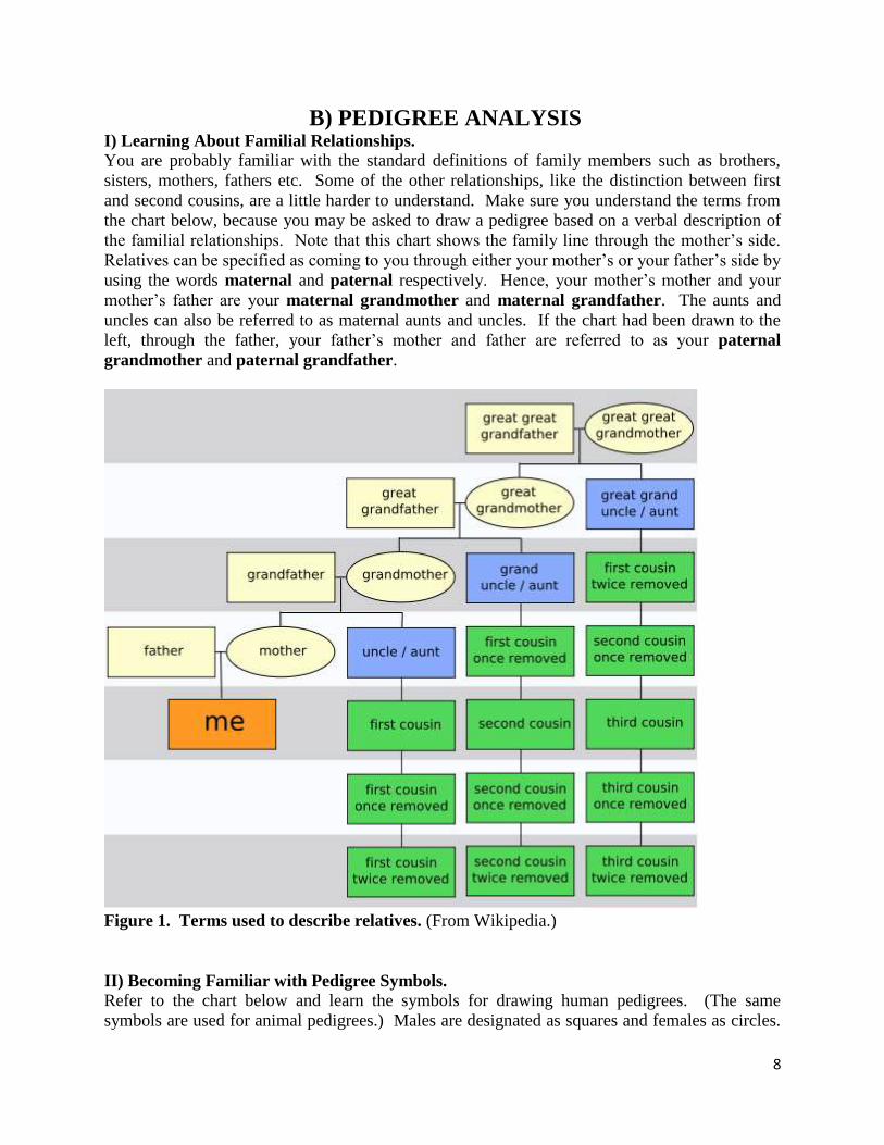
B) PEDIGREE ANALYSIS I) Learning About Familial Relationships.

You are probably familiar with the standard definitions of family members such as brothers,

sisters, mothers, fathers etc. Some of the other relationships, like the distinction between first

and second cousins, are a little harder to understand. Make sure you understand the terms from

the chart below, because you may be asked to draw a pedigree based on a verbal description of

the familial relationships. Note that this chart shows the family line through the mother’s side.

Relatives can be specified as coming to you through either your mother’s or your father’s side by

using the words maternal and paternal respectively. Hence, your mother’s mother and your

mother’s father are your maternal grandmother and maternal grandfather. The aunts and

uncles can also be referred to as maternal aunts and uncles. If the chart had been drawn to the

left, through the father, your father’s mother and father are referred to as your paternal

grandmother and paternal grandfather.

Figure 1. Terms used to describe relatives. (From Wikipedia.)

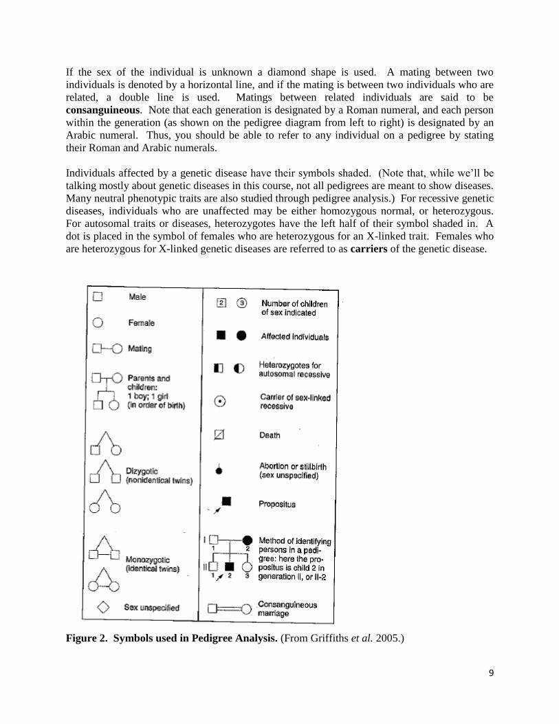
II) Becoming Familiar with Pedigree Symbols.

Refer to the chart below and learn the symbols for drawing human pedigrees. (The same

symbols are used for animal pedigrees.) Males are designated as squares and females as circles.

9

If the sex of the individual is unknown a diamond shape is used. A mating between two

individuals is denoted by a horizontal line, and if the mating is between two individuals who are

related, a double line is used. Matings between related individuals are said to be

consanguineous. Note that each generation is designated by a Roman numeral, and each person

within the generation (as shown on the pedigree diagram from left to right) is designated by an

Arabic numeral. Thus, you should be able to refer to any individual on a pedigree by stating

their Roman and Arabic numerals.

Individuals affected by a genetic disease have their symbols shaded. (Note that, while we’ll be

talking mostly about genetic diseases in this course, not all pedigrees are meant to show diseases.

Many neutral phenotypic traits are also studied through pedigree analysis.) For recessive genetic

diseases, individuals who are unaffected may be either homozygous normal, or heterozygous.

For autosomal traits or diseases, heterozygotes have the left half of their symbol shaded in. A

dot is placed in the symbol of females who are heterozygous for an X-linked trait. Females who

are heterozygous for X-linked genetic diseases are referred to as carriers of the genetic disease.

Figure 2. Symbols used in Pedigree Analysis. (From Griffiths et al. 2005.)

10

Figure 3. A Typical Pedigree Showing Autosomal Recessive Diseases. (From Griffiths et al

2005).

A typical pedigree is shown in figure 3. Note that each generation is indicated by a Roman

numeral and each individual within a generation is indicated by an Arabic numeral so that every

person can be referred to by these numbers. Note the consanguineous marriage between III-5

and III-6. Interestingly, in this particular pedigree, two different recessive genetic traits are being

shown simultaneously. One trait is shown by shading the left side of the symbol, and the other

by shading the right half. Thus, individual IV-6 is affected by the recessive disease carried by

both of her parents.

III) Determining the Mode of Inheritance.

Dominant versus Recessive Genetic Diseases.

What causes a genetic disease (or any genetic trait for that matter) to be dominant versus

recessive? Many genetic diseases are caused by mutations to important enzymes. Complete

removal of the enzyme will lead to the recessive phenotype. Removal of both copies of the gene

would obviously lead to no enzyme being produced, leading in turn to the mutant phenotype.

But what happens when you still have one wild-type copy of the gene? Will the amount of

protein produced be enough to ‘hide’ the recessive phenotype? This is usually what determines

whether a gene mutation is recessive or dominant.

If the gene is physically removed (something called a deletion mutation), or if its promoter is

mutated so that it is not transcribed, no mRNA will be produced and the enzyme will be absent

altogether. This is called a null mutation. In other cases, the enzyme is produced in the same

amount, but it doesn’t work as efficiently, or it may do something slightly different from the

wild-type protein. (Mutations that cause changes in the amino acid composition of the enzyme

will do this, for example.) A mutation that causes an enzyme to be absent or to not work as well,

so that the wild-type phenotype changes to the mutant phenotype is called a loss of function

11

mutation. Similarly, a mutation either to a second gene or to the same one that causes the

mutant phenotype to revert to the wild-type phenotype is called a gain of function mutation.

A heterozygote will have both the functional and the mutant version of the protein. If the

functional protein being produced from the wild-type gene is enough to compensate for the

mutant protein, the genetic disease will be recessive. This means that the presence of the

functional gene can ‘hide’ or ‘cover up’ the non-functional one. This also means that half the

normal amount of enzyme is enough to do the job. In this case, one dose of the gene is said to be

haplosufficient. Examples of human autosomal recessive genetic diseases are

phenylketonuria, cystic fibrosis,Tay-Sachs disease and sickle cell anemia. In all cases,

having one functional copy of the gene is enough to cover up the presence of the mutant version.

On the other hand, if having half the amount of the wild-type protein being produced is not

enough to compensate for the effects of the mutant or absent protein, the enzyme dosage is said

to be haploinsufficient, and a mutant phenotype results. This means that the mutant phenotype

will appear even though there is one functional copy of the gene present. In this case the genetic

disease is dominant, and the mutation is said to be a dominant or dominant negative mutation.

There are even some cases where the mutant protein is worse than nothing, and can actually

interfere with the function of the wild-type protein. This is a special kind of mutation called an

antimorphic mutation. (An example might be a mutant enzyme that catalyzes a reaction, but

then fails to let to of the products afterwards.) This too would result in a dominant genetic

disease. Thus, be aware that a genetic mutation can cause a mutant phenotype either because

half the dosage of the functional protein is haploinsufficient, or because the mutant protein is

antimorphic. Examples of dominant human genetic diseases are pseudoachondroplasia

(dwarfism, also referred to as achondroplasia), Huntington disease, and polydactyly (extra

fingers and toes).

There are other examples of genetic traits that are neither completely dominant nor completely

recessive. In the case of incomplete dominance the phenotype of the heterozygote is

somewhere in between the phenotype of the homozygous wild-type and the homozygous mutant.

In the case of codominance, the phenotypes conferred by both alleles are visible in the

heterozygote. The ABO blood grouping system is an example of this, where the AB phenotype

is clearly distinguishable from the AA and BB phenotypes. We will not be using codominance

or incomplete dominance in pedigree analysis in this course.

Determining The Most Likely Mode of Inheritance.

One of the first steps in studying a genetic disease is to determine its mode of inheritance. In this

course we’ll limit the choices to autosomal dominant, autosomal recessive, and X-linked

recessive. It is usually easiest to start by determining whether the disease is dominant or

recessive, and then moving on to determining whether it is autosomal or X-linked. Furthermore,

it is more definitive to eliminate one of the two possibilities as being impossible, and then

assume it must be the other, unless there is also evidence that argues against that one as well.

Here are some characteristics to look for.

12

Dominant versus Recessive.

Some patterns to look for right away that can give you a clue about whether the trait is dominant

or recessive are as follows. Dominant genetic diseases are present in every generation, and

effected children can only come from effected parents. Recessive genetic diseases can skip

generations, and it is possible for effected children to come from non-effected parents. Here are

some specific examples of things to look for to help you deduce the mode of inheritance as being

either dominant or recessive.

1. For an autosomal dominant disease, it is possible for two effected parents to have an

uneffected child. This is absolutely impossible with an autosomal recessive disease.

Furthermore, when you see this happen, you know that both parents must be heterozygotes. ie-

If you had assumed that the disease was recessive, and used allelic symbols A and a to denote the

alleles, with A being the wild-type, and a being the mutant, then both parents must be the

homozygous recessive aa. If this were the case, they couldn’t produce a child that was either Aa

or AA to get the wild-type phenotype. However, if this were a dominant disease, and you used

D and d as allelic symbols, with D being the dominant negative mutation, then getting the wild-

type phenotype in II-1 would mean the parents must both be of the Dd genotype.

Autosomal Dominant Inheritance Pattern.

13

2. For an autosomal recessive disease, it is possible for two uneffected parents to have an

effected child. This is absolutely impossible for an autosomal dominant disease. Furthermore, if

you see this happen, you know that both parents must be heterozygotes!

Autosomal Recessive Pattern:

3. When analyzing a pedigree that has a history of genetic disease, assume that people who

marry into the family are not carrying the disease allele. Assume they are homozygous normal.

If you see evidence that this is not the case, you may have to throw out the assumption. (Note,

this assumption only applies to genetic diseases because they are rare. Pedigrees are sometimes

used to study fairly neutral genetic traits, like blue eyes vs. brown eyes. Blue eyes are the

recessive phenotype, but obviously it would be unwise to assume that a brown-eyed person

marrying in to a family of blue-eyed people is homozygous dominant for the brown-eyed

alleles.)

Autosomal versus X-Linked Inheritance. Most X-linked genetic diseases are recessive. Hemophelia and red-green colour blindness are

two examples of recessive X-linked genetic diseases. Male pattern baldness is also an X-linked

recessive trait, which is why people say that baldness comes from your mother’s side of the

family. Some interesting patterns of inheritance operate through the X chromosome because,

while females have two X chromosomes, males only have one. Thus, the frequency of X-linked

genetic diseases is higher in men than in women because men do not have another X

chromosome to mask an X chromosome carrying a mutant allele. For example, red-green colour

blindness is ten times more common in men than in women.

Here are some other interesting facts about recessive X-linked disorders:

1. Generally, the disease affects men much more often than women. This can be seen from a

quick scan of the pedigree. Indeed, in order for a woman to be effected certain conditions have

to be met. In order for a daughter to be effected, her father must be effected, and her mother

14

must be either effected or a carrier. Thus, if you see an effected daughter, and her father is not

effected, it can’t be an X-linked recessive genetic disease.

This Cannot be X-linked Recessive.

2. When a father is effected by an X-linked disease, he will pass it on to all of his daughters (but

none of his sons). Thus, all of the daughters of a colour blind father will be carriers for colour

blindness. If those daughters marry uneffected men, half of their sons will be effected and half

of their daughters will be carriers.

An effected father will give his effected X to all of his daughters.

3. A carrier mother will give her effected X chromosome to half of her sons and half of her

daughters. If the father is not effected, the daughters will be carriers, but all of the sons who

received the effected X will be effected. Thus, seeing half of the sons in a family being effected

by a genetic disease, while none of the daughters are effected is a clue that the disease is X-

linked recessive, and the mother is a carrier.

4. A female will only be effected by an X-linked recessive disease if she is homozygous

recessive. In this case all of her sons will have the disease. Thus, a family with an effected

mother and an uneffected father, in which all of the sons are effected but none of the daughters

(because they are carriers) is a sign of an X-linked recessive disease. So, for example, a colour

15

blind mother will have all colour blind sons, and all of her daughters will be carriers, provided

the father is not colour blind. Since the daughters are carriers, half of their sons will be colour

blind.

5. Having an effected father and a carrier mother will result in half the children of each sex being

effected. This is the only case in which an X-linked recessive disease can lead to equal numbers

of effected sons and daughters. Thus, if you see half the children of each sex being effected, and

the father is not effected, it can’t be an X-linked recessive disease.

Figure 4. An example of an X-linked Recessive Genetic Disease. (From Griffiths et al 2005)

Figure 4 shows a typical pedigree for an X-linked recessive genetic disease. See how III-1 was

able to inherit colour blindness from his maternal grandfather (I-2) through his carrier mother (II-

2). A dot is placed in the center of her symbol to indicate she is a carrier. In this particular

pedigree, the author has indicated the genotypes using X to indicate the X chromosome, with a

superscript (A or a) to indicate the alleles for colour blindness. The Y chromosome is also

shown, such that XAX

A indicates a homozygous normal female, X

aY indicates a colour blind

male, and so on.

IV) Determining the Odds of a Couple Having an Effected Child.

You are familiar with the single gene ratios from first class, where a mating of Aa and Aa gives

rise to aa one quarter of the time, a mating of Aa and aa gives rise to aa half the time and so on.

For a single gene genetic disease, these ratios can be used in conjunction with a pedigree to

calculate the odds of a couple having an effected child. This is done in two steps. First, look at

the parents and assume they’re heterozygotes (for an autosomal recessive disease, for example).

Then calculate the odds of them having an effected child assuming they are carriers. Second,

(and this is more complicated) you must determine the odds that they actually are carriers by

determining the genotypes of as many people in the pedigree as possible. The odds of the couple

having an effected child will be the product (multiplication) of the single gene ratio and the odds

that they actually are carriers. Consider the example below.

16

Let’s use A and a as gene symbols. The fact that I-1 and I-2 are unaffected, but have an effected

daughter (II-1) indicates a recessive inheritance pattern. This is also true for I-3 and I-4. The

fact that II-1 is affected but her father is not rules out the possibility of it being an X-linked

recessive disease. Thus, this disease is autosomal recessive. Now that you’ve decided this, you

can write aa beside II-1 and II-4.

Note that in order for I-1 and I-2 to have an effected daughter, they must both be heterozygotes.

Therefore, you can fill in half of their gene symbols, and write Aa beside each. The same is true

for I-3 and I-4. Now all we have to do is figure out how likely it is that II-2 and II-3 are carriers.

II-2 is not showing the disease, and you know that his parents are both heterozygotes. You must

calculate his odds of being a carrier (Aa). You know that his parents are both heterozygotes, and

you know that matings between heterozygotes give genotypic ratios of 1/4AA 1/2Aa and 1/4aa.

You might guess, therefore, that the odds of II-2 being Aa are 1/2, but this would actually be

wrong. True, an Aa X Aa mating will produce genotypes in the ratio of 1/4AA 1/2Aa and 1/4aa,

but, since you can actually see that II-2 is not aa, you have to throw out that possibility and re-

adjust the ratio knowing that he can only be AA or Aa. (This is also sometimes called

‘normalization’ or normalizing a ratio.) So, the two possibilities that are left occur in a ratio of

1/4AA and 2/4Aa, which, after adjustment, is the same as 1/3AA and 2/3Aa. Thus, the

possibility of II-2 being a carrier is 2/3! The same is true for II-3.

Therefore, if both II-2 and II-3 are carriers, the odds of them having an effected child are 1/4.

The odds of II-2 actually being a carrier are 2/3, and the odds of II-3 actually being a carrier are

2/3. Thus, by the ‘product rule’ the odds of the couple having an effected child are the product

of (1/4) (2/3) (2/3)=4/36. 4/36 reduces to 1/9. Therefore, you would tell this couple the odds are

one in nine that they will produce a child affected by the disease.

The procedure for calculating the odds of other types of genetic diseases can be adjusted

accordingly. So, for example, in order to calculate the odds of a couple having a colour blind

boy when the mother is not colour blind, you would have to determine the odds that she is a

carrier. If she is colour blind, the odds of having a colour blind boy are 100%.

Notice that for X-linked recessive diseases, if the father is not showing the disease, you know

that he is not carrying it, because males have no ability to hide recessive X-linked alleles. This

usually makes X-linked pedigrees much easier to analyze, because, in cases where the father is

17

not showing the disease, you only have to concern yourself with the mother’s side of the

pedigree.

Class Exercise in Determining Modes of Inheritance from Pedigrees.

Your instructor will divide you into six groups (one group for each table). Each group will take

ten minutes to analyze one of the following pedigrees. You should determine the mode of

inheritance, give gene symbols for the disease (for this exercise use an upper case letter for the

dominant allele and a lower case letter for the recessive one), and then fill in the genotypes of as

many people on the pedigree as you can.

1

.

18

2

3

19

4

5

20

6

After the class has gone through the pedigrees, try the five pedigrees that you did not do.

21

Class Exercise in Determining the Odds of Having an Effected Child from a Pedigree.

Determine the mode of inheritance of the genetic disease in the pedigree shown below, fill in the

genotypes of as many of the individuals as you can, and determine the odds that III-1 will be

effected by the condition.

Class Exercise in Drawing a Pedigree from a Description.

Example: Tay-Sachs disease (“infantile amaurotic idiocy”) is a rare human disease in which

toxic substances accumulate in nerve cells. The recessive allele is inherited in a simple

Mendelian manner. A woman is planning to marry her first cousin, but the couple discovers that

their shared grand-father’s sister died in infancy of Tay-Sachs disease. Draw the relevant parts

of the pedigree, and show all the genotypes as completely as possible. Calculate the probability

that the cousins’ first child will have Tay-Sachs disease. (Assume all people marrying into the

family are homozygous normal.)

22

SUPPLEMENTAL PEDIGREE PROBLEMS:

1. For the pedigree shown below, determine the most likely mode of inheritance, assign

genotypes to as many people on the pedigree as you can, and estimate the odds of V-1 being

effected by the disease.

23

2. For the pedigree shown below determine the most likely mode of inheritance, fill in the

genotypes of as many individuals as you can, and determine the odds that V-1 will be effected by

the disease.

24

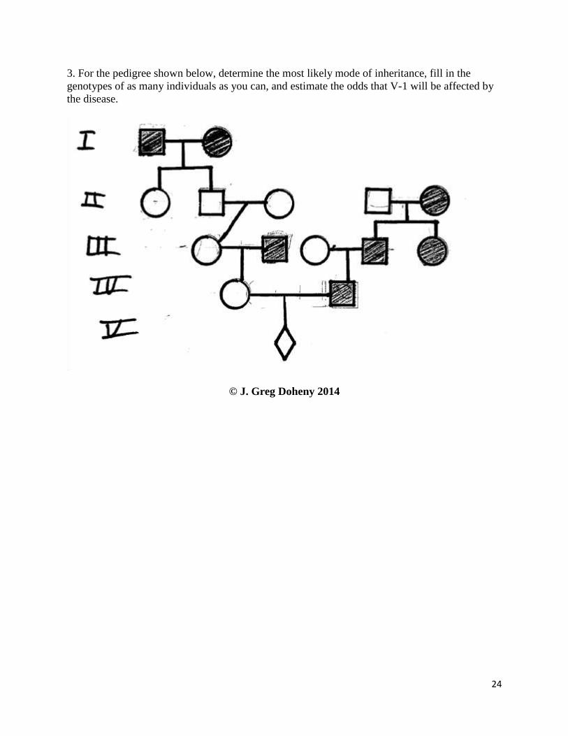
3. For the pedigree shown below, determine the most likely mode of inheritance, fill in the

genotypes of as many individuals as you can, and estimate the odds that V-1 will be affected by

the disease.

© J. Greg Doheny 2014