Notes on multidimensional scaling of distances in a ...jdvicto/jdv/riemds.pdf · Other symmetric spaces (the k-planes in n-space) acted on by SO(n) Non-Euclidean spaces, e.g., SL(n,¡

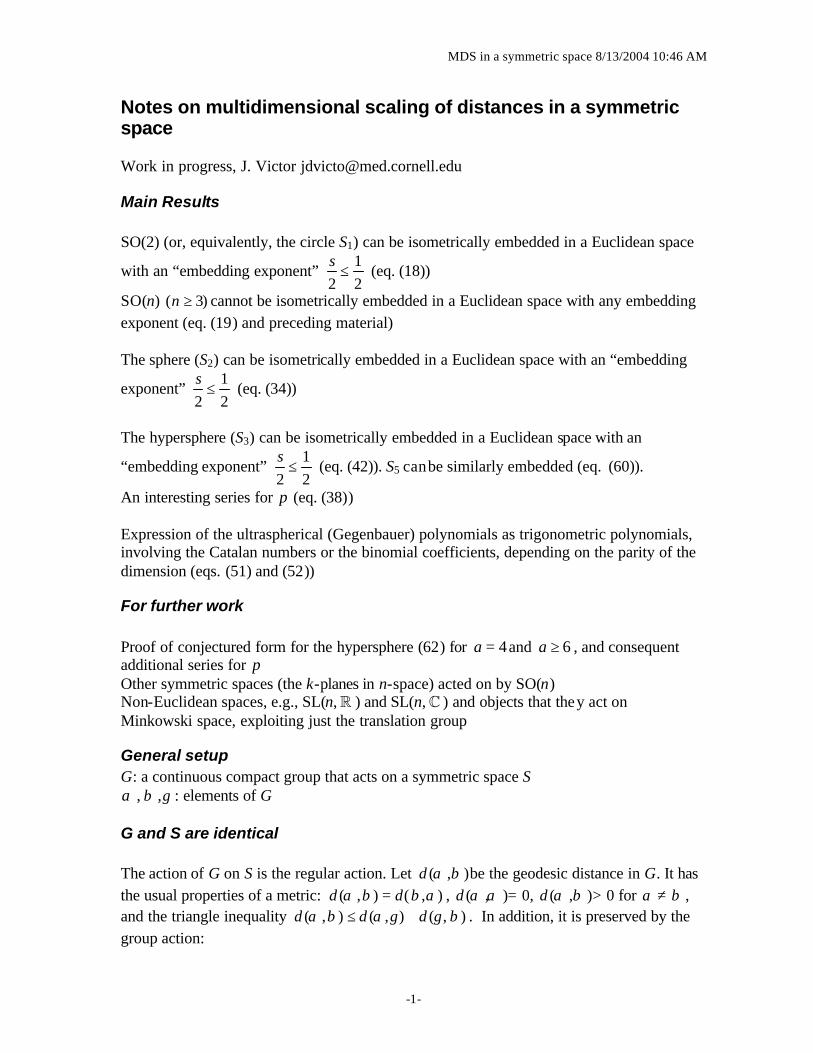
MDS in a symmetric space 8/13/2004 10:46 AM

-1-

Notes on multidimensional scaling of distances in a symmetric space Work in progress, J. Victor [email protected]

Main Results SO(2) (or, equivalently, the circle S1) can be isometrically embedded in a Euclidean space

with an “embedding exponent” 1

2 2s

≤ (eq. (18))

SO(n) ( 3)n ≥ cannot be isometrically embedded in a Euclidean space with any embedding exponent (eq. (19) and preceding material) The sphere (S2) can be isometrically embedded in a Euclidean space with an “embedding

exponent” 1

2 2s

≤ (eq. (34))

The hypersphere (S3) can be isometrically embedded in a Euclidean space with an

“embedding exponent” 1

2 2s

≤ (eq. (42)). S5 can be similarly embedded (eq. (60)).

An interesting series for π (eq. (38)) Expression of the ultraspherical (Gegenbauer) polynomials as trigonometric polynomials, involving the Catalan numbers or the binomial coefficients, depending on the parity of the dimension (eqs. (51) and (52))

For further work Proof of conjectured form for the hypersphere (62) for 4a = and 6a ≥ , and consequent additional series for π Other symmetric spaces (the k-planes in n-space) acted on by SO(n) Non-Euclidean spaces, e.g., SL(n, ¡ ) and SL(n, £ ) and objects that they act on Minkowski space, exploiting just the translation group

General setup G: a continuous compact group that acts on a symmetric space S α , β ,γ : elements of G

G and S are identical The action of G on S is the regular action. Let ( , )d α β be the geodesic distance in G. It has the usual properties of a metric: ( , ) ( , )d dα β β α= , ( , ) 0d α α = , ( , ) 0d α β > for α β≠ , and the triangle inequality ( , ) ( , ) ( , )d d dα β α γ γ β≤ + . In addition, it is preserved by the group action:


-2-

( , ) ( , ) ( , )d d dαγ βγ γβ γα α β= = . (1)

We want to relate the distance to a Euclidean distance, by mapping each group element α to a vector 1 2( ( ), ( ),... ( ),...)kx x xα α α , so that

2( ( , )) ( ( ) ( ))k kk

f d x xα β α β= −∑ , (2)

some monotonic function f. For reasons discussed in Aronov and Victor (2004), we will only consider ( ) sf d d= , where / 2s is the “embedding exponent.” That is

( )1/2

/ 2 2( , ) ( ( ) ( ))s

k kk

d x xα β α β

= − ∑ . (3)

The dimension of the embedding, and hence the number of terms in the sum, is typically infinite. That is, our goal is to recapitulate d exactly for all elements α , β of G via this Euclidean distance. This is in contrast to a more common viewpoint, in which the goal is to approximate d with a small number of dimensions. [Indyk, P., and Matousek, J. Low Distortion Embeddings of Finite Metric Spaces, in Handbook of Discrete and Computational Geometry, 2nd. Ed., editors: Goodman, J.E., and O'Rourke, J., in press (2004). CRC Press LLC, Boca Raton, FL.]

Let ,

1( (0, )) ( ( , )) ( (0, ))

G GG

f d f d f d dGβ α β

µ β α β β β∈ ∈

= = = ∫ , (4)

where denotes an average with respect to the invariant measure, the integral is also

taken with respect to the invariant measure on G, and G

G d β= ∫ .

Following Kruskal’s approach for multidimensional scaling, we write

,

1 1 1 1( , ) ( ( , )) ( ( , )) ( ( , )) ( ( , ))

2 2 2 2G G GF f d f d f d f d

γ γ γ γα β α β α γ γ β γ γ

′∈ ∈ ∈′= − + + − ,

which, because of the symmetries, becomes 1

( , ) ( ( , ))2

F f dα β α β µ= − + . (5)

Equation (2) is now equivalent to

( , ) ( ) ( )k kk

F x xα β α β= ∑ . (6)

We can assume that ( ) 0k Gx

αα

∈= , and replace ( )kx α by

2

( )( )( )

kk

kG

xyx

γ

ααγ

∈

= , so that

our goal is to write


-3-

( , ) ( ) ( )k k k

k

F y yα β λ α β= ∑ (7)

for orthonormal functions ky on G. This is equivalent to finding the eigenvalues kλ and eigenfunctions yk of an integral operator: 1

( , ) ( ) ( )k k kG

F y d yG

α β β β λ α=∫ .

Diagonalization

( , )F α β is a function on G G× . An orthogonal basis for such functions are the matrix elements of all the irreducible representations of G G× . These are parameterized by a pair ( , )ρ σ , where both ρ and σ are irreducible representations of G. Say

1 2( )m mρ α is a typical

matrix element of ρ (for m1 and m2 in [1,…, dim ρ ]) and similarly for 1 2

( )n nσ β .Thus,

1 2 1 2 , 1 2 1 2,

( , ) ( ) ( ) ( , , , )m m n nF F m m n nρ σρ σ

α β ρ α σ β= ∑ % . (8)

Since

1 2 1 2 1 1 2 2

1( ) ( )

dimm m n n m n m ng

ρσα

ρ α σ α δ δ δρ∈

= , (9)

it follows that

1 2 1 2, 1 2 1 2,

( , , , ) dim dim ( , ) ( ) ( )m m n nG

F m m n n Fρ σα β

ρ σ α β ρ α σ β∈

=% . (10)

Via a change of variables α γβ= , it follows that

1 2 1 2, 1 2 1 2,

( , , , ) dim dim ( , ) ( ) ( )m m n nG

F m m n n Fρ σβ γ

ρ σ γβ β ρ γβ σ β∈

=% ,

from which the fact that ρ is a group representation, and eq. (1), imply

1 2 1 2

dim

, 1 2 1 21 ,

( , , , ) dim dim (0, ) ( ) ( ) ( )m r rm n nr G

F m m n n Fρ

ρ σβ γ

ρ σ γ ρ γ ρ β σ β= ∈

= ∑% .

The average over β can now be computed separately, via eq. (9):

2 1 2 1 2 2

1( ) ( )

dimrm n n rn m nG ρσβ

ρ β σ β δ δ δρ∈

= . (11)

Thus,

1 11 2 1 2,( , , , ) dim (0, ) ( )m n

GF m m n m F

ρ ρ γρ γ ρ γ

∈=% , (12)


-4-

and , 1 2 1 2( , , , ) 0F m m n nρ σ =% unless σ ρ= and 2 2n m= . To calculate the quantity in eq. (12), we break down the average over the group into an average over conjugate classes, parameterized by θ , weighted by the volume ( )h θ of each conjugate class ( )c θ :

1 1 1 1 ( )(0, ) ( ) (0, ) ( ) ( )m n m n

G cF F h d

γ γ θγ ρ γ γ ρ γ θ θ

∈ ∈= ∫ .

The property (1) implies that 1(0, ) (0, )F Fθ νθν −= , so (0, ) (0, )F Fγ θ= for any ( )cγ θ∈ .

Moreover, the average of ρ over a conjugate class ( )c θ commutes with any ( )ρ α and has trace ( )

ρχ θ , from which it follows that

1 1 1 1( )

1( ) ( )

dimm n m nc

ργ θ

ρ γ δ χ θρ∈

= .

Therefore,

1 1 1 1

1(0, ) ( ) (0, ) ( ) ( )

dimm n m nG

F F h dργ

γ ρ γ δ θ χ θ θ θρ∈

= ∫ . (13)

Note that since (0, ) 0G

Fγ

γ∈

= (as a consequence of eq. (5)), eq. (13) is zero for the trivial

representation. Combining eqs. (5), (12), and (13) yields

1 2 1 2,

1( , , , ) ( ( ,0)) ( ) ( )

2F m m m m f d h dρρ ρ

θ χ θ θ θ= − ∫% , (14)

and , 1 2 1 2( , , , ) 0F m m n nρ σ =% unless σ ρ= , 1 1n m= , and 2 2n m= . Therefore, the irreducible representation ρ contributes 2(dim )ρ orthogonal functions ky ,

one for each matrix element 1 2m mρ . In view of eq. (11), ( ) 1 2

dim ( )m mρ ρ α are orthonormal.

Thus, comparing eq. (7) and (8), all of these 2(dim )ρ eigenvalues are equal to

1 2 1 2,

1 1( , , , ) ( ( ,0)) ( ) ( )

dim 2dimF m m m m f d h dρ ρρ ρ

θ χ θ θ θρ ρ

Λ = = − ∫% . (15)

Parseval relation From the orthonormality of the yk , it follows from eq. (6) that

22 2

,( , ) ( ,0) k

G G k

F Fα β α

α β α λ∈ ∈

= = ∑ . (16)

Note that 2 2 2 24 ( ,0) ( ( ,0) ) ( ( ,0)

G G GF f d f d

α α αα α µ α µ

∈ ∈ ∈= − = − . (17)


-5-

Applications We carry out this program for SO(n).

SO(2) Elements of the group, and conjugate classes, are parameterized by an angle [ , ]θ π π∈ − . Irreducible representations are parameterized by an integer n ∈Z (both positive and negative), with ( ) in

n e θχ θ = . Representations are one-dimensional. The weight of a

conjugate class θ is 1

( )2

h θπ

= .The distance is given by ( ,0)d θ θ= .

With ( ) sf d d= , eq. (15) yields

0

1 1( ) cos( )

2 2 2s si n

n

ds e n d

π πθ

π

θθ θ θ θ

π π−

Λ = − = −∫ ∫ .

For 1s > , this expression becomes negative for sufficiently large even values of n, thus indicating that a Euclidean embedding is not possible. Specializing to 1s = yields

2

1(1)n nπ

Λ = (n odd) and (1) 0nΛ = (n even). (18)

For the Parseval relation (with 1s = ), 2π

µ = ,2

2 21( ( ,0))

2 3Gf d d

π

απ

πα θ θ

π∈−

= =∫ ,

22 2( ( ,0))

12Gf d

α

πα µ

∈− = ,

and (recalling that terms from n and –n contribute) the familiar series 4

4 4 4

1 1 1...

96 1 3 5π

= + + + is recovered from (16).

SO(3) Conjugate classes, are parameterized by an angle [0, ]θ π∈ , the angle of rotation. Irreducible representations are parameterized by an integer 0n > . The nth irreducible representation is the action of G on homogeneous polynomials ( , , )p x y z of degree n for

which 2 0p∇ = . It is of dimension 2 1n + , and has character ( )n

imn

m n

e θχ θ=−

= ∑ . The weight

of a conjugate class θ is 1 cos

( )hθ

θπ

−= . The distance is given by ( ,0)d θ θ= .

With ( ) sf d d= , eq. (15) yields


-6-

( )0 0

1 1 cos 1( ) cos( ) cos(( 1) )

2(2 1) 2 (2 1)

ns sim

nm n

s e d n n dn n

π πθ θ

θ θ θ θ θ θπ π=−

− Λ = − = − − + + +

∑∫ ∫. For 0s > , this expression becomes negative for even values of n, thus indicating that a Euclidean embedding is not possible. Specializing to 1s = yields

2

1 1(1)

2 1n n nπΛ =

+ (n odd) and

2

1 1(1)

2 1 ( 1)n n nπΛ = −

+ + (n even). (19)

For the Parseval relation (with 1s = ), 2

2π

µπ

= + ,

22 2

0

1( ( ,0)) (1 cos ) 2

3Gf d d

π

α

πα θ θ θ

π∈= − = +∫ ,

22 2

2

4( ( ,0))

12Gf d

α

πα µ

π∈− = − , and again the familiar series

4

4 4 4

1 1 1...

96 1 3 5π

= + + + is

recovered from (16).

Setup for G and S distinct We posit a map φ from G to S ,and d is a distance in S. The property (1) is replaced by

( ( ), ( )) ( ( ), ( ))d dφ γβ φ γα φ α φ β= . (20)

The circle S1 This is identical to S=G=SO(2); G and S are not distinct.

The sphere S2 We use the setup with an explicit map φ from G to S, not the “coset” setup. The right-hand version of property (1) is not used until after eq. (12). Using eq. (20) rather than eq. (1) , we evaluate eq. (12) as follows: G=SO(3). The map φ from G to S2 takes Gα ∈ to the point ˆ( )zα on S2 to which α moves the north pole z . The distance is given by 1 ˆ ˆ( ( ), ( )) cos ( ( ) ( ))d z b zφ α φ β α−= • . We will parameterize the distances by θ . Eq. (20) is satisfied, since

1 1 1ˆ ˆ ˆ ˆ ˆ ˆ( ( ), ( )) cos (( )( ) ( )( )) cos ( ( ( )) ( ( ))) cos ( ( ) ( ))d z b z z b z z b zφ γα φ γβ γα γ γ α γ α− − −= • = • = • . The nth irreducible representation is the action of G on homogeneous polynomials

( , , )p x y z of degree n for which 2 0p∇ = . A basis for these polynomials consists of the

spherical harmonics ( , )mnY θ ϕ where { },...,m n n∈ − , and


-7-

2 1 ( )!

( , ) (cos )4 ( )!

m m imn n

n n mY P e

n mϕθ ϕ θ

π+ −

=+

, (21)

where ( )mnP u is an associated Legendre polynomial [Eric W. Weisstein. "Spherical

Harmonic." From MathWorld--A Wolfram Web Resource. http://mathworld.wolfram.com/SphericalHarmonic.html]. 0 ( ) ( )n nP x P x= is the nth Legendre polynomial, orthogonal on [ 1,1]− , satisfying

1

1

2( )

2 1nP x dxn−

=+∫ . (22)

From eqs. (5) and (12), for nontrivial representations ρ we have

1 11 2 1 2,

dim( , , , ) ( (0, )) ( )

2 m n GF m m n m f d

ρ ρ γ

ργ ρ γ

∈= −% . (23)

and (from eq. (15))

1 11 2 1 2,

1( , , , ) ( (0, )) ( )

2 m n Gm m n m f d

ρ ρ γγ ρ γ

∈Λ = − . (24)

All matrix elements of ( )ρ γ contain a nontrivial dependence on ie φ except the one in the

row and column corresponding to 0 2 1( , ) (cos )

4n n

nY Pθ ϕ θ

π+

= . We arbitrarily choose this

to be the first row and column of ( )ρ γ . Moreover, the average in eq. (23) can be replaced by an average over all products ξγ , where ξ is a rotation by an angle φ about the north pole z .Thus, the average in eq. (23) must be zero except at 1 1 1m n= = . Another consequence of the above argument is that the average in eq. (23) can be replaced by an average over the angle θ by which γ moves the north pole z , i.e.,

ˆ ˆ( ) cos( ( ) ) (0, )z z dθ γ γ γ= • = . The weight associated with this angle θ is

1( ) sin

2w θ θ= (

0

( ) 1w dπ

θ θ =∫ ), (25)

since any final position of ˆ( )zγ on S2 is equally likely. For a rotation γ that moves the north pole z by an angle θ , the (1,1) matrix element of

( )ρ γ is

1,1( ) (cos ( ))nPρ γ θ γ= . (26) This conforms to the normalization (eq. (9)) of matrix elements of group representations:

2 2 2

1,10

1( ) (cos ) (cos ) ( )

2 1n nG

P P w dn

π

γρ γ θ θ θ θ

∈= = =

+∫ , (27)


-8-

where the last equality follows from eqs. (22) and (25). Combining eqs. (23),(25), and (26), and taking ( ) sf d d= yields

,0

2 1(1, ,1, ) (cos )sin

4s

n

nF m m P d

π

ρ ρ θ θ θ θ+

= − ∫% , (28)

where the average over Gγ ∈ has been replaced by an average over ( )θ γ . Thus, the nth irreducible representation of SO(3) contributes 2 1n+ terms to eq. (8) (for

{ }1,...,2 1m n∈ + in eq. (28)), and an eigenvalue ( )n sΛ of multiplicity 2 1n + to eq. (16). In view of (15),

0

1( ) (cos )sin

4s

n ns P dπ

θ θ θ θΛ = − ∫ . (29)

Evaluation of this integral is facilitated by writing the Fourier series

, ,1 1

(cos ) cos( ) cos( )2 ! 4

n n

n n q n qn nq n q n

P b q B qn

θ θ θ=− =−

= =∑ ∑ , (30)

where ,n qb and ,n qB are nonzero only for 2q n r= − . Note that both negative and positive frequencies are included. One can show (see Appendix I) that

( ) ( )

2

, 2 2 2

! ( 2 2 )!(2 )! (2 )!22 !2( )! !2

n n r n n

nrn n r r n

bnnn r rr

−

− = = −

, (31)

or equivalently, that

, 2 2

( )! ( )!

! !2 2

n qn q n q

Bn q n q

+ −=

+ −

. (32)

For 1s = , the above integral (29) can then be evaluated from the Fourier series, since

2

0

, 11

cos sin, 1

4

qq

q dq

ππ

θ θ θ θπ

> −=

− =

∫ , (33)

for odd 1q ≥ . (For n even, the integral (29) is zero, since (cos )sin2 nPπ

θ θ θ −

is odd-

symmetric around 2π

θ = , and 0

cos sin 0q dπ

θ θ θ =∫ .)

Appendix II shows that


-9-

2

22 2 2 2

0

1 ( 1)!(1) (cos )sin

1 14 2 2! !2 2

n n mn n

nP d C

n n

π π πθ θ θ θ + +

− Λ = − = =

− +

∫ , (34)

where 2 1n m= + and mC is the mth Catalan number

2(2 )! 1!( 1)! 1m

mmC

mm m m

= = + + . (35)

[Sloane citation A000108, http://www.research.att.com/projects/OEIS?Anum=A000108].

To apply the Parseval relation (16) (for 1s = ), note that 2π

µ = , and, with ( ( ,0))f d θ θ= ,

that

( )2 2

2

0

1sin 2

2 2 4d

π π πθ µ θ θ θ − = − = −

∫ , (36)

where 1

sin2

θ is the weight associated with a point on S2 at polar angle θ .

With these, eqs. (16) and (17) give 2 2

44 4

2 1

1(2 1)

16 2 2 mnn m

n Cπ π

+= +

− = +∑ . (37)

This can be re-arranged to 4

2 42 1

8 2 11

2 mnn m

nC

π = +

+− = ∑ . (38)

Left and right-hand sides are both approximately 0.18943.

The hypersphere S3 Here, G=SO(4). Analogous to the case of S2, The map φ from G to S3 takes Gα ∈ to the point ˆ( )zα on S3 to which α moves z , and the distance is given by

1 ˆ ˆ( ( ), ( )) cos ( ( ) ( ))d z b zφ α φ β α−= • . The irreducible representations of G are parameterized by a pair of integer indices, g+ and g-, corresponding to the largest Fourier coefficients with respect to 1 2ω ω+ and

1 2ω ω− present in the characters, where 1ω and 2ω are the principal angles of the rotation of a typical group element Gα ∈ . All matrix elements of , ( )g gρ γ

+ −contain a nontrivial

dependence on a rotation about z , of the form ie φ except for one. That one is the matrix element in , ( )n nρ γ that corresponds to transformations of the homogeneous polynomial of

degree n that depends only on cosz θ= . The dimension of , ( )n nρ γ , which describes the


-10-

transformation of all homogenous polynomials of degree n (including those that do not depend only on z), is

23 1( 1)

3 3n n

n+ +

− = +

.

Denote the polynomial that depends only on z by (cos )nQ θ . These polynomials must be orthogonal with respect to the weight

22( ) sinw θ θ

π= (

0

( ) 1w dπ

θ θ =∫ ). (39)

Since 1

( ) (1 cos(2 ))2

w θ θ= − , it follows that

(cos ) cos( )n

n na n

Q K aθ θ=−

= ∑ , (40)

where only terms for which a n≡ (mod 2) are included. nK can be determined from eq. (11), as follows:

( ) ( ) ( )2 2 22

0 0

1 1(cos ) ( ) (cos ) 1 cos(2 )

( 1) n n nQ w d Q d Kn

π π

θ θ θ θ θ θπ

= = − =+ ∫ ∫ ,

so 1

1nKn

=+

.

Again, the average corresponding to eq. (24) can be replaced by an average over the angle θ by which γ moves z , weighted by ( )w θ . This is because any final position of ˆ( )zγ on S3 is equally likely, and the points at angle θ correspond to the surface of an S2-sphere of radius sinθ . Thus, the irreducible representation of SO(4) corresponding to ( , ) ( , )g g n n+ − = contributes

2( 1)n + terms to eq. (8), and an eigenvalue ( )n sΛ of multiplicity 2( 1)n + to eq. (16). In view of (15),

2

0 0

1 1( ) (cos ) ( ) (cos )sin

2s s

n n ns Q w d Q dπ π

θ θ θ θ θ θ θ θπ

Λ = − = −∫ ∫ . (41)

For 1s = ,

2 2

4(1)

( 2)n n nπΛ =

+. (42)

To apply the Parseval relation (16) (for 1s = ), note that 2π

µ = , and, with ( ( ,0))f d θ θ= ,

that

( )2 2

2 2

0

2 1sin

2 12 2d

π π πθ µ θ θ θ

π − = − = − ∫ , (43)


-11-

where 22sin θ

πis the weight associated with a point on S3 at polar angle θ . Eq. (16), eq.

(42), eq. (43), and the fact that the multiplicity of (1)nΛ is 2( 1)n + lead to

2 2 2

4 42 1

( 1)( 1)

128 6 ( 2)n m

nn n

π π

= +

+− =

+∑ . (44)

This is equivalent to the sum of the following two series for π attributed to Euler (Xavier Gourdon and Pascal Sebah, http://numbers.computation.free.fr/Constants/Pi/piSeries.html):

2

2 31

3 1 164 2 (4 1)k kπ ∞

=

− + =−∑ (45)

and 4 2

2 41

30 1 1768 2 (4 1)k k

π π ∞

=

+− =

−∑ . (46)

(Prior to February 2004, that there had is a typographical error in eq. (45) on the above website).

The hypersphere Sa Here, G=SO(a+1). 1a = corresponds to the circle, 2a = corresponds to the sphere, and

3a = corresponds to the hypersphere. The map φ from G to aS takes Gα ∈ to the point ˆ( )zα on aS to which α moves z , and the distance is given by

1 ˆ ˆ( ( ), ( )) cos ( ( ) ( ))d z b zφ α φ β α−= • .

The irreducible representations of G are parameterized by an 1

2a +

-tuple of integer

indices. The dimension of the representation which describes the transformation of all homogenous polynomials of degree n (including those that do not depend only on z), is

2n a n aa a+ + −

−

. (47)

Denote the polynomial that depends only on z by , (cos ).n aR θ These polynomials must be orthogonal with respect to the weight

1 1

1( )

2( ) sin sin( )2

a aa a

a

w Aa

θ θ θπ

− −

+Γ

= =Γ

, (48)


-12-

where ( 1)0

1a aA

M −= (eq. (54)) o ensure that 0

( ) 1w dπ

θ θ =∫ . (49)

Polynomials for Sa The needed polynomials can be written in terms of the Gegenbauer polynomials. The Gegenbauer polynomials ( ) ( )nC xλ are orthogonal on [-1,1] with respect to the weight

2 1/2(1 )x λ−− . With ( ) ( )1( )n nD x Cλ λ

λ= and cosx θ= , ( ) (cos )nD λ θ are orthogonal with respect

to 2sin λ θ on [0, ]π . So, other than a scale factor, 1

( )2

, (cos ) (cos )a

n a nR Dθ θ−

= , Standard formulae (Abramowitz and Stegun chapter 22), imply that for 0λ >

( )2

1

1 1( ) 1

(1 2 )n

nn

D x txt t

λλλ

∞

=

= − − +

∑ , ( )0

1D λ

λ= ,

and

(0) 2

1

( ) log(1 2 )nn

n

D x t xt t∞

=

= − − +∑

and

( )1 22( ) 2

20

2 ( 2 )(cos ) sin

( ) ( 1) ( 1)n

nD d

n n

π λλ λ λ

θ θ θ πλ λ

− Γ +=

+ Γ + Γ +∫ provided 0n > or 0λ > .

Writing 2(1 2 ) (1 )(1 )i ixt t te teθ θ−− + = − − , along with the generating function, shows

(0) 2( ) cos( )nD x n

nθ= .

We want to determine the coefficient of ( , , )V n cµ of ice θ in ( /2) (cos )nD µ θ . Straightforward algebra provides the double generating function

( /2) 2

0, 0

( 1) ( ) 2log( 1 2 )mn

m

D x t y y xt tµ µ µ

µ

∞

= =

− = − + − +∑ ,

where the sum includes all nonnegative integer pairs ( , )mµ except 0mµ = = .

( )2

0, 0,( , ) (0,0) 0

1( 1) ( , , ) 2log (1 )(1 )

2m i i ic

m m

V m c t y y te te e dπ

µ µ θ θ θ

µ µ

µ θπ

∞− −

= = ≠

− = − + − −∑ ∫ .

Put iz e θ= .

10, 0,( , ) (0,0)

1( 1) ( , , ) 2log (1 )(1 )

2m

cm m

t dzV m c t y y tz

i z zµ µ

µ µ

µπ

∞

+= = ≠

− = − + − −

∑ ∫ ,

with the contour integral sur rounding 0.


-13-

Noting that 112 1

1

1 1 ( 1)2

aa

aaa

uu C

∞+

−−=

+ = + −∑ , we have

1 12 1 2 11 , 1, 1

1 1(1 )(1 )

2 2k a b

a ba bk a b k a b

ttz t z C C

z

∞−

− −− −= + = ≥ ≥

− − = ∑ ∑ .

Alternatively, let

1( ) ( 2 ) ( )

2 2( )2 1

( ) ( 1) 4 ( 1) ( ) ( )2 2

pa

p pa p a

f ap p a

a a p

+Γ + Γ + Γ

= =+ +

Γ Γ + Γ + Γ Γ (50)

(via duplication formula for the gamma function), the coefficient in the Taylor series / 2

0

(1 ) ( )p jp

a

x x f j∞

−

=

− = ∑ .

It follows by equating coefficients in the generating functions that

( /2) (cos ) ( , , )m

p icm

c m

D V m p c e θθ=−

= ∑ (51)

where the summation is only for m c≡ (mod 2) and 2

( , , ) ( ) ( )2 2p p

m c m cV m p c f f

p+ −

= for 0p > , (52)

and, in the limit that p approaches 0, 1

( ,0, ) ( , )V m c c mm

δ= so that (0) 2 1(cos ) cos( ) ( )im im

mD m e em m

θ θθ θ −= = + for 0m > .

The normalization is

( )12( /2)

20

2 ( )(cos ) sin

( ) ( 1) ( 1)2 2

pp p

mm p

D dp p

m m

π

θ θ θ π− Γ +

=+ Γ + Γ +

∫ , (53)

again provided 0m > or 0p > . Since the above quantities are undefined for 0, 0m p= = , we arbitrarily take

(0,0, ) ( ,0)V c cδ= so that (0)0 1D = , so

( )2(0)0

0

(cos )D dπ

θ θ π=∫ .

Note 0 ( ) ( ,0)f j jδ= (the circle), 1 2

1 (2 )!( )

4 ( !)j

jf j

j= (the sphere), 2( ) 1f j = (the hypersphere,

as required for eq. (40)), and 4( ) 1f j j= + .

For 1,p = ,

2( ,1, )

4 m cmV m c B= (eq. (32)), and (1/2) (cos ) 2 (cos )n nD Pθ θ= (eq. (30)).


-14-

Moments for Sa

Write ( )

0

sinp j pjM d

π

θ θ θ= ∫ . Via integration by parts and elementary calculations, we find

( ) ( 2)0 0

1p ppM M

p−−

= , (0)0M π= , (1)

0 2M = , and hence

( )0

1( )

2

( 1)2

p

p

Mp

π

+Γ

=Γ +

(54).

Similarly, ( ) ( 2)1 1

1p ppM M

p−−

= , ( ) (0)1 12

pM Mπ

= , and hence

( ) 3 /21

1( )

2

2 ( 1)2

p

p

Mp

π

+Γ

=Γ +

,

and ( ) ( 2) ( 2)2 2 02

1 2p p ppM M M

p p− −−

= − , and hence

for p even:

5/2( )2 2 2 2

1( ) 1 1 12 2 ...

3 ( 2) 2( 1)2

p

p

Mp p p

ππ

+Γ

= − + + + − Γ +

for p odd:

5/2( )2 2 2 2

1( ) 1 1 12 2 ...

2 ( 2) 1( 1)2

p

p

Mp p p

ππ

+Γ

= − + + + − Γ +.

Thus, the variance required for the right side of eq. (17), (or eq. (36)) is

( )( )

2( )1( )

2 2( ) ( )10 0

1 12

2

pp

p pm

MM

M M p m

∞

=

− = +

∑ , which is equivalent to

for p even (using 2

2 2 2

1 1 1...

24 2 4 6π

= + + + ):

( ) 2( ) 21( )

2( ) ( ) 2 2 20 0

1 1 1 12 ...

12 2 4

pp

p p

MM

M M pπ − = − + + +

, (55)


-15-

for p odd (using 2

2 2 2

1 1 1...

8 1 3 5π

= + + + ):

( ) 2( ) 21( )

2( ) ( ) 2 2 20 0

1 1 1 12 ...

4 1 3

pp

p p

MM

M M pπ − = − + + +

. (56)

Eigenvalues The nth eigenvalue in dimension a is given by

0

1( ) (cos ) ( )

2s

n ns Q w dπ

θ θ θ θΛ = − ∫

where w is given by eq. (48) and where (cos )nQ θ is a multiple of 1

( )2

a

nD−

satisfying

( )2

0

1 1(cos ) ( )

2dimn an

Q w dn a n a

a a

π

θ θ θρ

= =+ + −

−

∫ .

From eq. (53) and (48),

21 2( )2

0

2 ( 1) 4 ( 1)(cos ) ( )

1 1 (2 1) ( ) ( 1)( ) ( ) ( ) ( 1)2 2 2

a a

n a

n a n aD w d

a a a n a a nn n

π πθ θ θ

− − Γ + − Γ + −= = − + + − Γ Γ + + Γ Γ Γ +

∫ ,

where the second equality follows from the standard duplication formula,

2 1/21 1(2 ) 2 ( ) ( )

22zz z z

π−Γ = Γ Γ + .

Thus,

1/2

1( )

2

(cos ) (2 1) ( ) ( 1) ( ) ( 1)2 ( 1)2

(cos ) 4 ( 1)

na

n

Q n a a n a nn an a n a

D n aa a

θ

θ−

+ − Γ Γ + Γ Γ + = = Γ + − + + − Γ + − −

.

Thus, it remains to find the coefficients in an orthogonal expansion of θ , i.e.,


-16-

1

0 0

1( )1 ( ) ( 1) 2( ) (cos ) ( ) ( , 1, ) sin

2 4 ( 1) ( )2

ns ic a

n n ac n

aa n

s Q w d V n a c e dan a

π πθθ θ θ θ θ θ θ

π

−

=−

+ΓΓ Γ +

Λ = − = − −Γ + − Γ

∑∫ ∫

where again the summation is only over terms for which c n≡ (mod 2). This also holds for 1a = , since V has appropriate limiting behavior.

In view of eq. (52) 1 1

2( , 1, ) ( ) ( )

1 2 2a a

n c n cV n a c f f

a − −+ −

− =−

,

and eq. (50) 1

1( )

2( )1

( ) ( 1)2

a

ar

f ra

r−

−Γ +

=−

Γ Γ +, (again using the duplication formula),

4 1

0

1 1( ) ( )( 1) ( 1) 2 2( ) 2 sin

( 1) ( 1) ( 1)2 2

nsa ic a

nc n

a n c a n ca n

s e dn c n cn a

πθθ θ θ

π− −

=−

− + + − + −Γ Γ− Γ +

Λ = −+ −Γ + − Γ + Γ +

∑ ∫ ,

where again the summation is only over terms for which c n≡ (mod 2). [Verified by riemds_a.m for s=1.] This can be rearranged, via a binomial expansion for

1 1 ( 1 2 )11sin ( ) ( 1)

2 ( 2 )

i ia a h i a h

ah

ae ee

hi i

θ θθθ

−− − − −− −

= = −

∑ and a change of variables c b h= + :

,| | 1 | | 1,| |

11

( ) ( ) ( )18 ( 1)

2 2

hn a n s

b a n h a b h n

n as i Z b h Y bn b h a h

n aπ ≤ + − ≤ − + ≤

− Λ = − +− − − − Γ + −

∑ ∑ , where

sums require 1b a n≡ + − , h b n≡ + (mod 2),

0

( ) s ibsY b e d

πθθ θ= ∫ ,

and

,

1 1( ) ( 1)

2 2a n

a n b h a n b hZ b h a

− + + + − + − − + = − Γ Γ

, whose arguments are half-

integer when a is even, and integer when a is odd. The factor ( 1)a − is absorbed into Z to ensure that behavior is finite for 1a = . For 1s = , the only nonzero terms are for n odd. [Verified by riemds_b.m for general s and n]. Consider

,| | 1,| |

1( , , ) ( )1

2 2

ha n

h a b h n

n aS a n b i Z b hn b h a h

≤ − + ≤

− = +− − − −

∑ (57)

and the associated generating function


-17-

, ,

ˆ( , , ) ( , , )( 1)

a n b

a n b

S S a n bn

α η βα η β =

Γ +∑

where the sums are over integers 1a ≥ , 1n ≥ , and all integers b.With

12

au

−= ,

2n b

p+

= ,2

n bq

−= ,

2h

t = ; u, p, q, t integer if a is odd; or half- integer if a is

even:

( )2 1

, , ,

2 (2 1) ( ) ( )ˆ( , , ) ( 1)( 1) ( 1) ( 1) ( 1)

qpu t

t u p q

u u q t u p t uS

u t u t q t p tη

α η β α ηββ

+ Γ + Γ − + Γ + += − Γ − + Γ + + Γ − + Γ + +

∑ ,

where max( , ) min( , )u p t u q− − ≤ ≤ . This reduces: 2

2 1 2 (2 1) ( )ˆ( , , ) ( 1)( 1) ( 1) (1 )(1 )

t tu t

uut u

u u uS

u t u tβ β

α η β αη ηββ

− −+

≤

Γ + Γ= −

Γ − + Γ + + −−∑ ,

2 22 1 2

2

2ˆ( , , ) 2 ( )1

u

u

u

S u uβ β

α η β αη

ηβ ηβ

−+

− + − = Γ − − +

∑

where again the sum is over half- integers 0u ≥ . From this, equating coefficients, we find the recursion relation:

( , , ) ( , 1, 1) ( , 1, 1) ( 1) ( , 2, )S a n b nS a n b nS a n b n n S a n b− − + − − − + − −

( )( 3)( 1)( 2, , 2) 2 ( 2, , ) ( 2, , 2)

4a a

S a n b S a n b S a n b− −

= − − − + − − − +

[verified with riemds_sanbr]. Taking

1 1( , , ) ( 1) ( , , )

2 2a a

S a n b n T a n b+ − = Γ + Γ Γ

one finds

( , , ) ( , 1, 1) ( , 1, 1) ( , 2, )T a n b T a n b T a n b T a n b− − + − − − + − ( 2, , 2) ( 2, , ) ( 2, , 2)T a n b T a n b T a n b= − − − + − − − +

[verified with riemds_tanbr]. Then,

( 1) ( 1)2( , , )1 1( 1) 1

2 2 2

n b

b nb a a n

T a n b ib n a n b a n bn

−

+ Γ − Γ + − =− + + + + − +Γ + Γ + Γ Γ

,


-18-

provided 2a ≥ and 0b ≥ , and is 0 if b n< with n even (a odd), consistent with the pole in the denominator. This can be seen to satisfy the above recursion relation, and also to agree with eq. (57) for 1b n a= + − and 3b n a= + − [verified with riemds_tanb]. Thus,

| | 1

1 1( 1)

2 2( ) ( , , ) ( )8 ( 1)n s

b a n

a an

s T a n b Y bn aπ ≤ + −

+ − Γ + Γ Γ Λ = −

Γ + − ∑ or

2

0 1

1( ) ( )22( ) . .

1 14 12 2 2

n b sn

b a n

b nabY b

s i c cb n a n b a n bπ

−

≤ ≤ + −

+ + ΓΓ Λ = − +

− + + + + − + Γ + Γ Γ

∑ (58)

with 1a n b+ + ≡ (mod 2) in all sums[verified with riemds_c]. For analytic results, specialize to 1s = . For a odd, n and b must be odd, and

1 2

2( )

iY b

b bπ

= − .

1

0 1

( )2 . .1 11

2 2 2

n b

b a n

b nbY b

i c cb n a n b a n b

−

≤ ≤ + −

+ Γ + =

− + + + + − + Γ + Γ Γ

∑

2

1

11( ) 4

( 1) ( )2 1( ) 1 2

n b

n b a n

b n a nn

a n bn a bn

−

≤ ≤ + −

+ + − −Γ − −+ + − Γ + − ∑ , making use of the conjugate

symmetry. From this and eq. (58), 2

2

1

11( ) 1 ( 1)

(1) 2 1( ) 2 1 2

n b

nn b a n

b n a nn a

a n bn a b nπ

−

≤ ≤ + −

+ + − − Γ + − Λ = Γ + + − Γ + − ∑ . (59)

For 1a = , eq. (18) is recovered. For 3a = , eq. (42) is recovered. For 5a = ,

2 2 2

64(1)

( 2) ( 4)n n n nπΛ =

+ +. (60)

This suggests the formula 21

2 2 2 2

2 1 1(1)

2 ( 2) ( 4) ...( 1)

a

n

an n n n aπ

− + Λ = Γ + + + − , (61)

which may be written 2

1( ) ( )1 2 2(1)

14 ( )2

n

a n

n aπ

+ Γ Γ Λ = + + Γ

. (62)

This appears to hold for not only for a odd but also for a even [riemds_d].


-19-

For a even, eq. (62)can be rewritten without Γ -functions (using

( )1( ) 2 1 3 ... (2 1)2

cc cπ−Γ + = • • • − as

2

21

1 1! !12 2 2 2(1) 1 1 14 4!2 2 2 2

12

n n a n a

a na n a na n

a n n a n a

n

π π+ +

− − − − Λ = =− + − + − −

.

For 2a = , this reduces to eq. (34). For 4a = , this becomes

21

9 1(1) 14 ( 1)( 3)

2n n

nnn n

π − Λ = − + +

.

Series for pi The series for π that follow from the Parseval relation (using the multiplicities (47), eq. (17), and eq. with 1p a= − )for 4a = is:

4

2 4 3 42 1

180 1 ( 2)(2 3)

1 216 19 2 ( 1) ( 3)

2n

n m

nn n

nn nπ = +

− + + − = − + +

∑ ,

and, for 2a = (equivalent to (38)), 4

2 4 42 1

18 1 (2 1)

1 16 12 ( 1)

2n

n m

nn

nnπ = +

− + − = − +

∑ .

In general, for a even, n and b must be odd, and 1 2

2( )

iY b

b bπ

= − .

Other symmetric spaces The sphere Sa can be regarded as the set of rays in (a+1)-dimensional space. It has a parameters, and is acted on by G=SO(a+1). G acts transitively on the sphere. The geodesics are obvious, namely, the trajectory taken between two given rays by a group action. The arc length distance is 1 ˆ ˆ( ( ), ( )) cos ( ( ) ( ))d z b zφ α φ β α−= • .


-20-

Consider the signed subspace defined by a k-tuple of vectors v1, …, vk in an n-dimensional space. The same subspace is defined by any nonsingular linear transformation of these vectors with positive determinant. (k=1, n=a+1 corresponds to Sa, above). The dimension of the space is k(n-k), as follows: To specify a k-dimensional subspace, choose k vectors in the n-dimensional space (nk dimensions). The space of interest is a quotient space of this k-fold product space by the general linear group on the k chosen vectors (any linear transformation of them leads to the same element of the symmetric space).

2 ( )nk k k n k− = − . My “planesph.m” and “planesph_inv.m” implement this mapping. The distance between an element described by a set of unit vectors v1, …, vk and a second set of unit vectors w1, …, wk is ( )1( , ) cos det j kd v w v w−= • . Note that a space, and the

same subspace with an odd permutation of the vectors, is considered maximally different, and just like sign inversion of one of the vectors. This is analogous to the fact that the antipodal points on a sphere are maximally different. One can also make a new symmetric space by identifying them with each other. To carry out the above program, one needs to, decompose ( )1cos det ( )j kv vα− • in terms of

irreducible representations of the group element α . In the case of S2, at eq. (23) and analogously for S3, we used the fact that all but one of the matrix elements of an irreducible rotation have a dependence on the polar angle, via ie φ . That angle could not influence the distance. But in the more general case, it is not yet clear whether the same logic applies. This should be testable empirically (at least if there is a dependence). A dependence seems likely, in that the distance between the index subspace and its image under α should depend not only on how far the polar axis z is moved, but also, on the movement of other vectors. However, there is a short cut that allows one to see that these spaces are embeddable, if Sr

is, for 1n

rk

= −

. This is because the k-spaces in an n-dimensional space can be mapped

into the 1-spaces in a space of dimension nk

via the antisymmetric tensor product. The

map preserves the above distance. This map is typically not onto. For example, for 4n = and 2k = the space of planes has 4 parameters, but is mapped into S5, the five-

parameter surface of a sphere in 6-dimensional space. Numerical experiments suggest (riemds.m, riemds_subdim_show.m) that indeed, not all of the embedding dimensions in S5 are needed for 4n = and 2k = . However, the embedding exponent still must be 1s = , since this space is at least as complicated as 3n = and 1k = .


-21-

More elegant setup, G and S distinct We posit a subgroup H of G, and consider S to be the space of right cosets. The map φ from G to S is the standard map from an element g to the coset gH. G acts transitively on S, and the stabilizer of any element of S is H. We allow d to act on G, and not just the coset space; diagonalizing d on G will is an equivalent problem. The property (1) is replaced by the slightly more restrictive

( , ) ( , )d dγβ γα α β= for Gγ ∈ because of the assumed symmetry of S (63) and

( , ) ( , )d dαη βη α β= for Hη ∈ because of the coset construction. (64) Since the property (1) is not used until after eq. (12), we still have (from eqs. (5) and eq. (12)), for each irreducible representation ρ of G :

1 11 2 1 2,

dim( , , , ) ( (0, )) ( )

2 m n GF m m n m f d

ρ ρ γ

ργ ρ γ

∈= −% . (65)

with 1 2 1 2,( , , , ) 0F m m n n

ρ ρ=% for 2 2m n≠ . That is, the diagonalization (8) has dim ρ copies

of a matrix dim

( (0, )) ( )2 G

B f dρ γ

ργ ρ γ

∈= − .

In view of eqs. (63) and (64), 1(0, ) (0, )d dγ η γη−= for Gγ ∈ and Hη ∈ . Therefore, 1 1 1( (0, )) ( ) ( (0, )) ( ) ( (0, )) ( )

G G Gf d f d f d

γ γ γγ ρ γ ηγη ρ γ ηγη ρ ηγη− − −

∈ ∈ ∈= =

and consequently, 1( ( )) ( )B Bρ ρρ η ρ η−=

That is, ( )ρ η commutes with Bρ for any Hη ∈ . Now, consider the further reduction of ρ to irreducible representations on H:

1 1 ( ) ( )... n nk k ρ ρρ ξ ξ= ⊕ ⊕ . The above commutation relationship implies that Bρ is a block-diagonal matrix on the

subspaces corresponding to each rξ . If 1rk = , it must be a multiple of an identity matrix of rank dim rξ within the subspace corresponding to rξ . For 1rk > , it is a matrix of rank

dimr rk ξ , composed of r rk k× blocks of arbitrary multiples of the identity matrix of rank dim rξ . But also, in view of eq. (64),

( )B Bρ ρ ρ η= for any Hη ∈ .


-22-

Therefore, the block matrix must be zero except within the space of rξ for which rξ is the trivial (identity) representation on H. In sum, there will only be contributions to the diagonalization for each irreducible representation ρ of G for which the restriction to H contains at least one copy of the identity matrix. If the number of copies is 1, then there will be a set of dim ρ identical eigenvalues in the diagonalization. If there are 1rk > copies, then it would appear that there can be up to 2

rk sets of dim ρ -tuples of identical eigenvalues. Note however that in the case of G S= (with H the identity element), further reduction is possible. Every irreducible representation of G contains the identity representation on H, in

dimk ρ= copies. But there are not 2k sets of dim ρ -tuples of identical eigenvalues, only k such sets. This is because ( )ρ η commutes with Bρ for any Gη ∈ , in view of the more

general property (1), and hence, Bρ must be diagonal.

Application of the more general formulation The above formulation indicates which irreducible representations can contribute to the diagonalization for the more general symmetric spaces. For the space of k-dimensional subspaces in an n-dimensional space, take SO( )G n= (with

1n a= + to correspond to the discussion of hyperspheres Sa) and SO( ) SO( )H n n k= × − .

Since the dimension of SO( )n is 1

( 1)2

n n − , it follows that the dimension of the space of

right cosets of H in G is k(n-k). Now we need to see how irreducible representations of G restrict to H.


-23-

Appendix I: Fourier series for Legendre polynomials of cosine argument We show by induction on n that

2 2

1 ( )! ( )!(cos ) cos( )

4! !

2 2

n

n na n

n a n aP a

n a n aθ θ

=−

+ −=

+ −

∑ , (66)

which, along with equation (30), is equivalent to eq. (32). We use a recurrence formula for the Legendre polynomials,

( )1 1

1( ) (2 1) ( ) ( )

1n n nP x n xP x nP xn+ −= + −

+ (67)

along with

( ) ( )( )1cos( )cos( ) cos ( 1) cos ( 1)

2a a aθ θ θ θ= + + − . (68)

Assuming that eq. (66) holds for all m n≤ , eqs. (67) and (68) imply that

( )1, , 1 , 1 1,

12(2 1)( ) 16

1n a n a n a n aB n B B nBn+ + − −= + + −

+. (69)

With u n a= + and v n a= − ,

, 2 2

! !

! !2 2

n au v

Bu v

=

.

Eq. (69) becomes

1, 2 2

( 1)!( 1)!

1 1! !

2 2

n au v

Bu v

+− −

= •+ +

( )2 2 2 21 1( 1)( 1) ( 1)( 1) ( 1) ( 1)

2 212

u v u vu u v v v u u v

u v+ + + + + + + + − + + + +

,

which simplifies to

( )1, 2 2 2 2

( 1)!( 1)! ( 1)!( 1)!( 1) ( 1)

1 1 1 1! ! ! !

2 2 2 2

n au v u v

B u u v vu v u v

+− − + +

= + + =+ + + +

, (70)

and completes the induction.


-24-

Appendix II: A combinatorial identity In view of eq. (33), eq. (34) is equivalent to

22 2 2 2

( )!( )!( , )

4 24 ! !

2 2

n

mnq n n

n q n qz n q C

n q n qπ π

+=−

+ −− =

+ −

∑ , (71)

where , as before, 2 1n m= + and is the mth Catalan number mC (eq. (35)), ( , ) 0z n q = unless

q n≡ (mod 2), 1

( ,1)4

z n = − , and 2

1( , )

1z n q

q=

−, otherwise. With 2 1q r= + and making

use of the fact that the summands depend only on q , this is equivalent to 2

22 2 2 2 2 2 2

1

1 ( 2 2)!(2 )! (2 2 2)!(2 2 )! 1 (2 )!2 ( 1)! ! ( 1)! ( )! 2 2 ( 1)! !

m

mr

m m m r m r mC

m m m r m r r r m m=

+ + + −− = =

+ + + − + +∑ . (72)

We verify (72) by a telescoping, based on 2

1 1 1 1( )

2 2 2 1r r r r= −

+ +. Note that the initial

term on the left of (72) is cancelled by the 1r

-component of the 1r = -term in the

summation. Thus,

2 2 2 2 21

1 ( 2 2)!(2 )! (2 2 2)!(2 2 )! 12 ( 1)! ! ( 1)! ( )! 2 2

m

r

m m m r m rm m m r m r r r=

+ + + −− =

+ + + − +∑

2 2 2 2 21

1 (4 2)! 1 1 (2 2 2)!(2 2 )! (2 2 )!(2 2 2)!2( 1) ( 2 1)! 2 ( 1)! ( )! ( ) ! ( 1)!

m

r

m m r m r m r m rm m r m r m r m r m r=

+ + + − + − +− − + + + + − + − +

∑ . (73)

We calculate

2 2 2 2

1 (2 2 2)!(2 2 )! (2 2 )!(2 2 2)!( 1)! ( )! ( )! ( 1)!m r m r m r m r

r m r m r m r m r + + − + − +

− = + + − + − +

( )2 22 2

1 (2 2 )!(2 2 )!(2 2 2)(2 2 1)( 1) (2 2 2)(2 2 1)( 1)

( 1)! ( 1)!m r m r

m r m r m r m r m r m rr m r m r

+ −+ + + + − + − − + − + + + =

+ + − +

( )2 2

1 (2 2 )!(2 2 )!4 ( 1)( 1)

( 1)! ( 1)!m r m r

r m r m rr m r m r

+ −+ + − + =

+ + − +

(2 2 )!(2 2 )!

4 4( 1)!( )( 1)!( ) m r m r

m r m rC C

m r m r m r m r + −+ −

=+ + + − + −

.

Thus, we can rewrite eq. (73) as


-25-

2 12 2 2 2 21 1

1 ( 2 2)!(2 )! (2 2 2)!(2 2 )! 12

2 ( 1)! ! ( 1)! ( )! 2 2

m m

m m r m rr r

m m m r m rC C C

m m m r m r r r + + −= =

+ + + −− = −

+ + + − +∑ ∑ . (74)

Finally, the desired identity (72) follows from the autoconvolution property of the Catalan numbers, which can be written in the form

22 1

1

2m

m m m r m rr

C C C C+ + −=

= + ∑ .

Appendix III: The axial component of generalized spherical harmonics [Supplanted via the use of Gegenbauer polynomials, above, with 1a k= + ] We determine relationships among families of orthogonal polynomials ( ) (cos )k

np θ ,

orthogonal (but not necessarily orthonormal) with respect to the weight 1

( ) sinkkw θ θ

π=

on the interval [ ]0,θ π∈ . We choose (0) (cos ) cosnp nθ θ= , and (1) (cos ) (cos )n np Pθ θ= ,

where (cos )nP θ is given by eq.(30). Consider ( )kp to be a column vector composed of ( ) (cos )k

np θ . Orthogonality of these polynomials corresponds to

( ) ( ) ( )

0

1( )

Tk k kkp p w d D

π

θ θπ

=∫ , (75)

for some diagonal matrix ( )kD . Since

( )22

1 cos2( ) sin ( ) ( )

2k k kw w wθ

θ θ θ θ+

− = =

, (76)

it follows that

( ) ( ) ( )2

0

1( )

Tk k kkp p w d T

π

θ θπ + =∫ , (77)

for a matrix ( )

,k

m nT whose only nonzero elements occur for m n= , 2m n= + , or 2m n= − . We work inductively, from k to 2k + , and attempt to find a matrix ( 2 )kA + of constants for which

( 2) ( ) ( 2) ( 2)k k k kp p A p+ + += + , (78) i.e.,

( 2) ( 2 ) 1 ( )( )k k kp I A p+ + −= − . (79) Substituting this into eq. (75) yields


-26-

( )( 2) ( 2) ( 2) ( 2) 1 ( ) ( ) ( 2) 12 2

0 0

( ) ( ) ( ) ( )Tk k k T k k k T k

k kD p p w d I A p p I A w dπ π

θ θ θ θ+ + + + − + −+ += = − −∫ ∫ , (80)

or, using eq.(77),

( 2) ( 2) ( 2) ( ) ( ) ( 2)2

0

( ) ( ) ( ) .k k k T k k T kkI A D I A p p w d T

π

θ θ+ + + ++− − = =∫ (81)

Equating matrix entries leads to

( 2) ( 2) 2 ( 2) ( 2), , 2 2, 2 ,( )k k k k

n n n n n n n nD A D T+ + + +− − −+ = (82)

and ( 2) ( 2) ( 2 )

2, , 2,k k k

n n n n n nA D T+ + ++ +− = . (83)

Example: k=0 For 0k = , (0) (cos ) cosnp nθ θ= . From eq. (77),

(2) 2 2,

0 0

1, 0

21 1 1 cos2 1 cos2 1

cos sin , 12 2 8

1, 2

4

n n

n

nT n d d n

n

π π θ θθ θ θ θ

π π

=

+ − = = = =

≥

∫ ∫

and

(2) 22,

0 0

1, 0

1 1 cos2( 1) cos2 1 cos2 4cos( 2) cos sin12 2 , 18

n n

nn

T n n d dn

π π θ θ θθ θ θ θ θ

π π+

− =+ + − = + = = − ≥

∫ ∫

From eqs. (82) and (83), (2)0,0

12

D = and (2)2,0

12

A = , and, for 1n ≥ , (2),

18n nD = and (2)

2, 1n nA + = ,

consistent with eq. (40). Note that the normalization factor is different than in eq. (40), since here, we are integrating only over θ , and not the entire sphere. Example: k=1 For 1k = , we choose and (1) (cos ) (cos )n np Pθ θ= , where (cos )nP θ is given by eq.(30). From eq. (77),

Acknowledgments


-27-

Thanks to John Velling for advice and Pascal Sebah for discussions related to series for π . Supported in part by NIH EY9314.

Documents

Notes on multidimensional scaling of distances in a ...jdvicto/jdv/riemds.pdf · Other symmetric spaces (the k-planes in n-space) acted on by SO(n) Non-Euclidean spaces, e.g., SL(n,¡