Notes on Exploration and Production Portfolio Optimization

-1-

Notes on Exploration and Production Portfolio Optimization

Ben C. Ball & Sam L. Savage

7/17/99

A New Era in Petroleum Exploration and Production ManagementExploration and Production (E&P) is the business of finding petroleum and getting it out of the ground. Itis a risky business in that most exploration projects are total failures while a few are tremendouslysuccessful. Thus the best possible management of risk is crucial.

In the 1930’s and 1940’s, the development of seismic data collection and analysis substantially reduced therisk in finding petroleum. The resulting geology and geophysics (G&G) revolutionized petroleumexploration. Decision analysis has traditionally been applied to the information derived from G&G to rankprojects hole by hole, determining on an individual basis whether or not they should be explored anddeveloped.

Today this “hole-istic” approach is being challenged by a holistic one that takes into account the entireportfolio of potential projects as well as current holdings. This portfolio analysis starts withrepresentations of the local uncertainties of the individual projects provided by the science and technologyof G&G. It then takes into account global uncertainties by adding two additional G’s: geo-economics andgeo-politics. It thereby reduces risks associated with price fluctuations and political events in addition tothe physical risks addressed by traditional G&G analysis. The holistic approach is based on but notidentical to the Nobel-prize winning portfolio theory that has shaped the financial markets over the pastfour decades.

Portfolio thinking in petroleum E&P is based on understanding and exploiting the interplay among bothexisting and potential projects. It does not provide all the answers, but encourages E&P decision-makersto ask the right questions, such as:

v If we want a long-term expected return of, say, 15% on our investment, how can we insure against acash flow shortfall over the first three years while minimizing our long-term risk?

v What should we pay for a new project, given the projects already in our portfolio? v How would oil projects, as contrasted from gas projects, affect the impact of price uncertainty on my

portfolio? v What projects should we be seeking to reduce the effects of political instability in a given part of the

world? v What are the effects on financial risk and return if we insist on a minimum of, say, 40% ownership of

any project? As we shall see, analytical models can help in directly addressing these and similar questions oncedecision-makers in the petroleum industry become comfortable with the holistic perspective.

History

The Financial Markets The story of quantitative portfolio analysis starts in the 1950s with the pioneering work of HarryMarkowitz, who formalized the insight that increased return generally implies assuming increased risk.His "efficient frontier" of stock portfolios described the optimal investments for investors with differingaversions to risk. His 1959 book on Portfolio Selection [1], remains an excellent introduction to this

© Ball & Savage Associates 1999 -2-

subject. In the 1960's William Sharpe [2] streamlined and expanded on Markowitz’s work with his CapitalAsset Pricing Model (CAPM), while Franco Modigliani and Merton Miller 3] made other importantcontributions to the theory of valuation of securities. In the early 1970's Fischer Black, Myron Scholes [4]and Robert Merton [5] determined a rational pricing principle for stock options. All of the researchersmentioned received Nobel prizes in economics for their discoveries1. The above body of work changed the face of Wall Street forever, resulting in the widespread acceptance ofan analytical approach to investing, and to the establishment of mutual funds, index funds, and derivativesecurities as common financial instruments.2 Today, many elements of this revolution are alreadyappearing in the energy markets.

Decision and Portfolio Analysis in Exploration and Production The approach described in this paper is derived from two sources: portfolio theory, as described above,and decision analysis. Decision analysis was first applied to E&P on a project by project basis by C. J.Grayson [6] and G. M. Kaufman [7], and popularized by A. W. McCray [8], P. D. Newendorp [9], R. E.Megill [10 and 11], J. M. Cozzolino [12], and others. In 1968 David B. Hertz [13] discussed theapplication of the Markowitz model to risky industrial projects as opposed to stocks. In 1983 an author ofthe present article [14] proposed that petroleum E&P strategy be based on the Markowitz model, anddiscussed examples based on mainframe computations. In a follow-up article Ball [14] proposed thedevelopment of efficient frontiers for E&P projects using personal computers. Since 1990 the two authorsof this article have collaborated on a sequence of models for consulting clients that have evolved to moreclosely reflect the differences between the stock market and E&P projects. Presentations to meetings of theSociety of Petroleum Engineers by Lee Hightower [16] and R. A. Edwards and T. A. Hewett [17] havealso reported on the application of financial portfolio theory to E&P. Hightower [18] authored a follow-uparticle in 1997. Also in 1997, Columbia University’s Lamont-Doherty Earth Observatory founded aconsortium of petroleum firms to share knowledge in the portfolio analysis of E&P projects [19]. Theinitial portfolio models used by this consortium, were developed by its director, John I. Howell, and werebased on the approach of the authors of this present paper as described below. The authors’ approach deals with the following primary differences between stock and petroleuminvestments. v Stock portfolios depend only on uncertain returns. E&P projects face both local uncertainties

involving the discovery and production of oil at a given site, and global uncertainties involvingprices, politics etc. Furthermore, uncertainties in stock returns usually follow a bell-shaped curvewhile E&P uncertainties are highly skewed and stress rare events.

v Risk in stock portfolios is usually measured in terms of volatility, the degree to which the portfolioswings in value. E&P portfolios must specifically track downside risk.

v The stock market is quite efficient3 whereas the market for E&P projects is inefficient.v E&P projects pay out over long time periods. Stocks can be bought or sold at will.v A stock portfolio generally contains a small fraction of the outstanding shares of any one company.

An E&P portfolio, on the other hand, often contains 100% of its constituent projects, creatingbudgetary effects.

1 The only exception being Black, who sadly passed away a few years before the prize was awarded for hiswork with Scholes. 2 For an excellent and very readable history of this revolution in the financial markets, see Capital Ideasby Peter Bernstein [24].3 The term “efficient” is used here in its technical, economic sense. An efficient market is one in which thereare no barriers to each item being priced at its actual value, as determined by all buyers and sellers, i.e.,there are no “bargains.”


This paper will show how we have dealt with each of the above issues. First a simple example will bepresented to build intuition into portfolio analysis.

Retraining Our Intuition Suppose you are responsible for investing $10 MM in E&P. Only two projects are available, either ofwhich would require the full $10MM for a 100% interest. One is relatively "safe," the other relatively"risky"4. The chances of success are independent. This information is reflected in the Table 1. This distribution of outcomes may also be displayed as histograms for each project as shown in Figures 1aand 1b. The expected net present value (ENPV) of each of the two projects can be shown to be the same asdemonstrated in Equations 1 and 2.

ENPVSafe = 60%*$50 + 40%*(-$10) = $26 MM Equation 1

ENPVRisky = 40%*$80 + 60%*(-$10) = $26 MM Equation 2

To attach a concrete risk to the outcomes, imagine that if you lose money you will also lose your job. It isclear that you have only a 40% chance of unemployment with the safe project, and a 60% chance with therisky one. Since they both have ENPVs of $26MM, you cannot increase your ENPV by investing in therisky project. Therefore, if you had to choose between one or the other project, the obvious and correctanswer is to invest the $10MM in the safe project.

The Diversification Effect But suppose you could split your investment evenly between the two projects. Intuition cautions againsttaking 50% of your investment out of the safe project and putting it in the risky one. However, let usexamine the four possible joint outcomes. Because the two projects are independent, the probability of anyparticular joint outcome is just the product of the probabilities of the associated individual outcomes. Notethat the sum of the probability column must be 100% as we have exhausted all possibilities, as shown inTable 2. The histogram for the resulting portfolio is displayed in Figure 2. This allocation of funds still provides an ENPV of $26MM. But now the only way you can lose money iswith two dry holes. Since the projects are assumed to be independent, the probability of two dry holes is40%*60% = 24%, cutting your risk of unemployment nearly in half! Intuition misleads: You can reducerisk by taking money out of a safe project, and putting it in a risky one. Although this answer is correct, itis not so obvious. This is known as the diversification effect, popularly referred to as not putting all your eggs in onebasket.5

One might consider this line of reasoning so fundamental that the petroleum industry would never dootherwise. However, the following summary of the conventional project selection process appeared in aDecember 1997 article in a leading professional petroleum exploration journal [20]: "Just rank explorationprojects by expected present worth.” This suggests that one should rank projects from the best to the worst and then select projects from the topdown until the budget is exhausted, ignoring the diversification effect. In the above example, this strategy

4 We shall have much to say about “risk” shortly. However, in every instance, we factors: the probability of an undesired outcome, and how undesirable that outcome is. 5 It is worth noting that the fact that the mass of the histogram of the 50/50 split has moved toward thecenter is related to the well-known central limit theorem of probability.


would have lead to allocating all of the funds to the “safe” project, which has the better risk reward ratio, butclearly this not the best portfolio. The authors’ experience with numerous E&P executives confirms that ranking “exploration projects byexpected present worth” is the norm. A majority of those informally surveyed favor investing 100% in the“Safe” project. A few are aware that a diversification of a portion of the portfolio into “Risky” will actuallyreduce risk, but even these are not aware of how to arrive at an optimal mix.

Shooting the Moon

Some E&P executives feel that a major discovery every decade or so can sustain a large company. Theymight claim that they prefer to “Shoot the Moon,” aiming for the highest possible expected return,regardless of the risk. The argument is that by ranking their projects in order of expected value, and thenmarching down the list until they run out of money, they will in fact arrive at the highest return/highestrisk point the efficient frontier.

This is simply not true. For instance, the company could add projects by borrowing, which would have theeffect of moving them to an even higher risk/higher return point than that achieved through ranking. Thushigh-grading does not deliver the highest point on the efficient frontier at all, but results in an arbitraryand unexamined tradeoff between risk and return.

We are not arguing that a company should explore with borrowed money. We are claiming that high-grading ignores a universe of other portfolios, both riskier and safer, that can be illuminated through ourapproach.

Measures of Risk Uncertainty is an inherent characteristic of our universe. Risk, on the other hand, is in the eye of thebeholder. The naïve measure of risk we have used above (the probability of getting fired) was chosen herefor illustrative purposes because it is easy to visualize and calculate. In practice, one would use a moresophisticated measure; for example, one that penalized larger losses more than small ones. However,diversification has a similar effect in reducing almost any sensible measure of risk. And, to the point here,full exploitation of the advantages of diversification are anything but intuitive. See Appendix 1 for afurther discussion of risk measures.

Statistical Dependence and Its Sources The above example assumes that the two projects are independent. In general, the interplay between twoprojects is more complex, in that their economic outcomes are interrelated. This is known as statisticaldependence. The simplest type of statistical dependence is correlation, which comes in two varieties. v Positive Correlation - A given outcome for one project increases the chance of an outcome in the

same direction for the other. This diminishes the effect of diversification.v Negative Correlation - A given outcome for one project decreases the chance of an outcome in the

same direction for the other. This enhances the effect of diversification. Let’s consider the effects of positive correlation on a 50/50 split between safe and risky. We assume thatthe individual distributions of “safe” and “risky” remain as above. Now, however, in the event that “safe”succeeds, “risky” is more likely to succeed, and in the event that “safe” fails, “risky” is more likely to fail. Thusthere is still a 40% chance that “safe” will fail, but if it does, the chance that “risky” fails is greater than 60%.Therefore the probability of losing your job is now greater than 24%. Next consider the effect of negativecorrelation. In the event that “safe” succeeds, “risky” is less likely to succeed, and in the event that “safe” fails,


“risky” is less likely to fail. Thus there is still a 40% chance that “safe” will fail, but if it does, the chance that“risky” fails is less than 60%. Therefore the probability of losing your job is now less than 24%. It isimportant to note that correlation affects only the risks. The expected value of $26MM remainsunchanged. In the portfolio approach, risk is managed by spreading the investments across a number ofopportunities while avoiding positive correlations and seeking negative correlations. It is possible to dothis optimally over numerous opportunities under diverse constraints, as the rest of the paper displays. It is easy to understand the importance of correlation when one considers a fire insurance policy on ahouse. Since the insurance has a positive ENPV to the insurer, we know it has a negative ENPV to theinsured, and is therefore a bad investment6. Statistical dependence may be due to many sources. The four listed below are not meant to be exhaustive,but are widely encountered in E&P projects.7

v Placesv Pricesv Profilesv Politics

Places The economic outcomes of two E&P sites in very close proximity (for example in the same field) will bepositively correlated through geological similarities, and would not constitute a very diversified portfolio.On the other hand two sites in widely distant locations will display little or no geological correlation, andhence would be more diversified. “Places” can have corresponding implications for pricing (especially gas)and political issues as well as for geologic ones.

Prices Petroleum projects produce crude oil and natural gas in various proportions. Crude oil prices generallytrack each other very closely worldwide. Thus, the economic outputs of oil projects worldwide arepositively correlated relative to fluctuations in crude price. However, this is not true for natural gas.Natural gas prices in many parts of the worldnotably in the United Statesdo not track either worldcrude oil prices or each other very well. Thus there would be a tendency for a portfolio consisting of a gasproject and an oil project to be less positively correlated and therefore better diversified, relative to price,than a portfolio consisting of two oil projects.

As an example of this phenomenon, The Wall Street Journal reported in 1993 [21] that the economy ofHouston, which had suffered during the crude oil price drop of 1986, had weathered a subsequent pricedrop successfully because it had diversified between oil and gas.

Profiles A frequent concern is the timing of the flows of various elements of projects, which may extend for manyyears into the future. These flows might include such elements as cash flow, hydrocarbon production,

6 Unless your portfolio also includes a house (whose value is of course negatively correlated to the value ofyour insurance policy). 7 Although we use “projects” throughout this paper, the same principles apply equally to E&P sites,exploration prospects, development projects, and/or acquisition properties. The point is that E&Pcompanies can add reserves in three ways: exploration, development (and redevelopment) and acquisition.Each has a very different risk/reward profile, the integrated analysis of which could reveal innovative,optimal portfolios. Most E&P companies isolate these three functions in their respective functional silosand, at best, suboptimize each. [25]


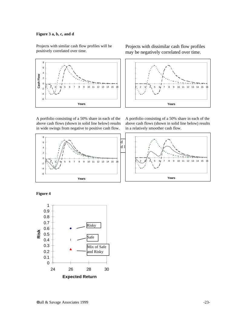
reserve additions, and staff requirements. Often the more nearly constant these flows can be, the better.The correlation among these elements can be taken into consideration to minimize fluctuations in cashflows. These critical factors that can literally make or break a company can now be considered andmanaged explicitly. As an example, consider how the correlations among project cash flows might be managed: Figure 3ashows the cash flow profile expected from two projects. If they were to comprise the portfolio, theresulting cash flow for the portfolio would be as shown in Figure 3b, with low valleys and high peaks.However, if two projects with expected cash flow profiles as shown in Figure 3c were to comprise theportfolio, the resulting cash flow for the portfolio would be as shown in Figure 3d. The peaks and valleysare leveled outa much more desirable cash flow profile.

Politics Petroleum investments have always been subject to political uncertainties, from the anti-trust decisionagainst Standard Oil of 1911 through environmental regulations, to the Gulf War of 1991 and beyond.Projects subject to disruption in the same direction due to the same political event will be positivelycorrelated. Negative correlation of projects may also be induced through political uncertainty. Forexample, consider two politically distinct regions that supply natural gas through two different pipelinesto a single market. The political disruption of production in either of the two regions could lead to marketshortages, and hence to increased prices and/or demands for the non-disrupted region. A portfolioconsisting of one project in each negatively correlated region would thus be protected, or “hedged,” againstpolitical risk in either region.

The Efficient Frontier We have seen that a combination of a safe project and a risky project can be less risky than a pureinvestment in the safe project. This is displayed graphically in Figure 4. In this example, there were onlytwo potential projects, and they had exactly the same ENPV. However, there will generally be projects ofvarious expected returns and risks as depicted in Figure 5. By calculating the minimum risk portfolio foreach of several levels of expected return, one can arrive at the curve shown in Figure 6. This curve showsthe optimum trade-off between risk and return and is known as the efficient frontier. Moving north from the efficient frontier increases risk without increasing expected return, while movingwest decreases expected return without decreasing risk. Since each point on the efficient frontier hasminimized the risk for that level of expected return, no portfolios exist to the southeast of the frontier.Thus the best portfolios are those on the efficient frontier itself. The concept of the efficient frontier andthe method of finding it were the fundamental Nobel Prize-winning contributions of Markowitz in the1950’s. No rational person would wish to be at any point above the efficient frontier. But which pointshould you pick? That depends on your firm’s willingness to suffer short-term volatility in the interest oflong-term growth. In E&P one may also develop additional frontiers showing optimal trade-offs betweenreserve additions, budget level, cash flow shortfall, or other meaningful metrics.

Important Differences Between Stocks and Petroleum Projects As mentioned earlier, the fundamental differences between stock returns and petroleum projects requiremodifications to the standard financial portfolio models. Some primary differences in the underlying assets are: v Types of Uncertaintiesv Risk Measuresv Nature of Marketsv Timing Considerationsv Budgetary Effects

-7-

Table 3 reviews these in more detail.

E&P Portfolio Optimization Model (EPPO)This section presents a simple E&P portfolio optimization model (EPPO), which unlike most standardfinancial portfolio models, can accommodate the characteristics of petroleum projects listed in Table 3.Excel versions of EPPO.xls may be downloaded from http://www-leland.stanford.edu/~savage orhttp://www.ziplink.net/~benball in formats for optimization with the Excel Solver, and What’sBest!®. As discussed earlier, the Markowitz and Sharpe models were intended for stock portfolios, and are notideally suited to portfolios of petroleum projects8. EPPO is based on two technologies already in wide useindividually in the petroleum industry: Monte Carlo simulation and linear programming. Here thesetechnologies have been combined to create a single period stochastic linear program [22]. The advantagesof this model for our purposes are: v It allows for arbitrary realistic probability distributions of project outcomes as opposed to multivariate

normal or log normal.v It supports a wide variety of risk measures.v It does not require historical data, but instead may be based on simulations, decision trees or other

types of inputv It estimates not just the mean and variance of the portfolio, but the entire distribution of outcomes EPPO works by feeding Monte Carlo trials into a linear program, which then finds a portfolio ofminimum risk for a given expected NPV. This process is repeated for a range of desired NPVs, therebydetermining the efficient frontier and the portfolios that comprise it.

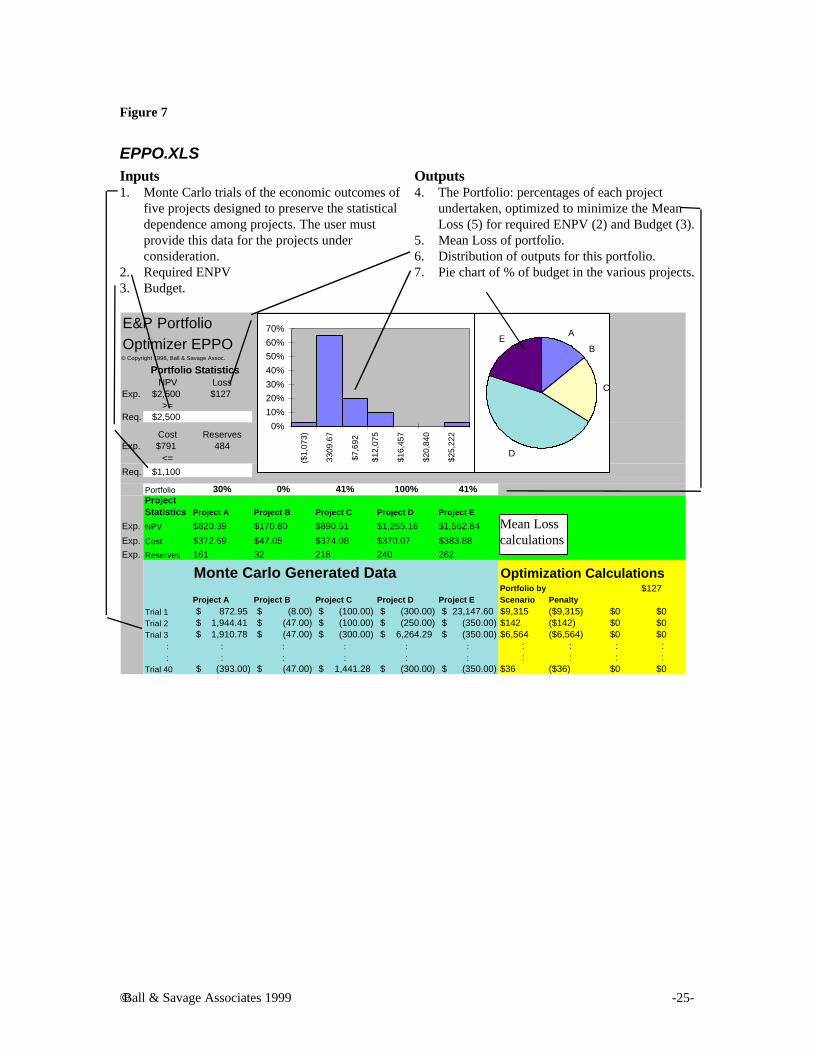
The Spreadsheet The basic elements of EPPO.xls are described in Figure 7. The program flow and underlying algebra aredetailed in Appendix 2. In the example shown here, the task is to optimize a portfolio from five exploration projects, A through E,given a particular budget.

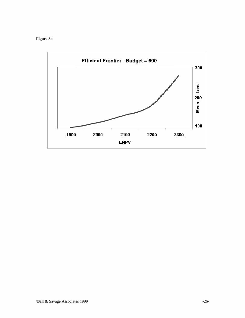
ResultsThe results shown in Figures 8 a, b, and c were produced by running the EPPO model with a budget of$600, and successive required ENPVs of $1900, $2000, $2100, $2200, and $2300. Figure 8a shows theresulting risk/return trade-off curve running from an ENPV of 1900 and a Mean Loss9 of 100 to an ENPVof 2300 and a Mean Loss of nearly 300. We refer to this curve as the Internal Efficient Frontier because itrepresents the best the firm can do with investments among its own projects. That is, each point on thisefficient frontier represents the highest expected value at that level of risk, or, equivalently, the lowest riskfor that expected value. There are no portfolios possible southeast of this frontier. All portfolios northwestof the frontier are inferior to a portfolio on the frontier, in that they offer an unnecessarily low returnand/or an unnecessarily high risk.

8 For comparison, a spreadsheet version of the Sharpe model is included in the solver example file thatships with Microsoft Excel. A Markowitz model is included with INSIGHT.xla [26] See alsowww.AnalyCorp.com.9 Mean Loss, as defined and described in Appendix 1, is a particularly simple risk measure. Other riskmeasures, as also described in Appendix 1, may be used.

-8-

A firm not applying portfolio analysis would be unlikely to be on such an internal efficient frontier. Wehave denoted such a position by X in Figure 8a. Such a firm could increase its expected return at constantrisk by moving to Z, or decrease its risk at constant return by moving to Y, or employ some intermediatestrategy.

For each level of ENPV, the stacked bars of Figure 8b show the makeup of the efficient portfolio for eachrequired ENPV. The vertical bars show the budget allocation to each of the five available projects in eachefficient portfolio. Figure 8c combines both of these graphs to show a complete picture of the risk returntrade-offs and the associated portfolios.

Management must choose such a point on the frontier, whereupon the underlying portfolio associated withthat point is revealed. For example, assume Management decided that at a budget of $600, an ENPV of$2,200 is needed and a Mean Loss of $171 is acceptable. Then portfolio analysis would reveal that thebudget should be allocated as follows to give the portfolio that would be most likely to yield thatperformance: 6% in Project A, none in Project B, 8% in Project C, 22% in Project D, and 64% in ProjectE.10

By contrast, current practice would be to decide separately on an investment level in each of the fiveprojects, based largely on the intrinsic merits of each. The resulting portfolio would likely be northwest ofthe internal efficient frontier, like the point “X” in the Figure 8a. The total risk would be higher thannecessary, or the expected value would be lower than necessary, ormost likelyboth.

Generalizing to multiple time periods One thing that EPPO and the Markowitz model do have in common is that both model current decisionsonly, based on potential future risks and rewards. A useful generalization would model both current andfuture decisions based on potential future risks and rewards. This would, in effect, be a marriage ofportfolio theory and real options theory, and might be accomplished through either multi-period stochasticlinear programming [22], or dynamic programming [23].

Business Implications: Asset Interplay Management The fundamental point of view of this paper is that project by project or “hole-istic” analysis misses manyimportant insights provided by the holistic perspective. The implications for the E&P business are thatmanagement must place at least as much emphasis on the interplay among projects as it does on theprojects themselves. We refer to this as Asset Interplay Management, and believe that it is currently notadequately exploited by the industry. Table 4 shows some examples of how various types of corporatedecision processes might be transformed by Asset Interplay Management. It is tempting to think of Asset Interplay Management as just another analytical tool or computer program.The danger in this view is that the tool or program will be adopted, and won’t deliver, thereby"inoculating" the company against a successful case of portfolio optimization for a generation ofmanagement. If the portfolio approach is to meet the expectations it is generating, top Management mustunderstand that it represents a fundamentally new way of thinking about the business of E&P. This willrequire:v Re-educating management, to develop and Asset Interplay Management until they become intuitivev Re-structuring corporate systems to collect and interpret stochastic data from a global as well as local

perspective

10 These “results” are no more than the results of a first iteration. For example, if 6% working interest inProject A is not practical, then the program should be rerun after placing the appropriate constraints onthe working interest in Project A, e.g., ≥ 10%. Such iterations should be continued until all “results” arewithin the realm of practicality. This, then, will represent the optimum practical portfolio, which, ofcourse, is the only one that matters in the real world.


v Revising reward programs to provide incentives for overall risk/reward positioning of the firm Each of the above implications of Asset Interplay Management is valuable in itself, and offers insights notavailable through project-by-project analysis. Each avoids some of the subtle but systemic errors to whichthe industry is presently vulnerable. But these are just first steps as E&P enters the dawn of this new styleof management. At the beginning of this article, we posed several questions that Management should be asking, but cannotadequately be answered without Asset Interplay Management. v If we want a long-term expected return of, say, 15% on our investment, how do we insure against a

cash flow shortfall over the first three years? Ø This would require determining the optimum portfolio while constraining the first three-year

cash flow to ≥ 0. v What should we pay for a new project, given the projects we already have in our portfolio?

Ø This could be determined by comparing the values of the portfolio with and without the newproject, but at constant risk. (This is almost certain not to be the project’s NPV.)

v How would oil projects, as contrasted from gas projects, affect the impact of price uncertainty on myportfolio? Ø Since Asset Interplay Management explicitly takes price interplay into account, the effect of each

project on the portfolio’s robustness relative to price instability can be determined. v What projects should we be seeking to reduce the effects of political instability in a given part of the

world? Ø Since Asset Interplay Management explicitly takes political interplay into account, the effect of

each project on the portfolio’s stability relative to political stability can be determined v What are the effects on financial risk and return of insisting on a minimum of, say, 40% ownership of

any project undertaken? Ø This would require determining the difference in portfolio value, at constant risk, with and

without the 40% constraint.

Conclusionsv Portfolio principles developed for the financial arena must be modified before application to E&P.v The portfolio perspective empowers decision-makers to focus on critical business issues, which guide

asset interactions, viz., places, price, profiles, and politics.v Portfolio management empowers decision-makers to manage risk, as well as measure it.v Changes in perspective, intuition, and culture will do more to promote Asset Interplay Management

than new computer programs. Modern portfolio theory provided the conceptual underpinning for the financial engineering that nowdominates Wall Street. How this will play out in the area of E&P remains to be seen. But one thing iscertain: Asset Interplay Management offers new and powerful tools for dealing head-on with one of theelements which distinguishes the upstream business, but which too long has been handled onlysubjectively: RISK.


Acknowledgements

We are indebted to several of our colleagues for reviewing this manuscript and formaking many helpful suggestions. We are especially grateful to Jerry Brashear, JohnHowell, and Dick Luecke for their extraordinary effort in making extremely detailedreviews, that resulted in many improvements in the finished work.

About the authors

Ben Ball and Sam Savage have a professional relationship dating from 1986. Since 1990 theyhave been working together in the area of portfolio optimization for petroleum exploration and productionprojects.

Ben C. Ball, Jr. is an internationallyrecognized petroleum expert. For twenty years he hasconsulted to several dozen firms on four continents,ranging from very small to extremely large, and toseveral governments and agencies—state, national, andinternational, in addition to serving as expert witness inseveral dozen cases. For the last twenty-two years hehas also held teaching and research appointments atM.I.T., including that of Adjunct Professor ofManagement and Engineering. Over 75 of his articleshave appeared in technical, professional, andmanagement journals and books, including HarvardBusiness Review, Petroleum Management, TechnologyReview, and the European Journal of OperationalResearch. His book, Energy Aftermath, which he co-authored with two M.I.T. colleagues, has beenpublished by Harvard Business School Press.

He received BS and MS degrees in chemicalengineering from M.I.T., and completed HarvardGraduate Business School’s Advanced ManagementProgram. He retired from Gulf Oil Corporation asCorporate Vice President after thirty years in operationsand planning.

P. O. Box 425158Cambridge, MA 02142-0004Phone 781/890-0939Fax 781/[email protected]://www.ziplink.net/~benball

Dr. Sam L. Savage is Director of IndustrialAffiliates for Stanford University’s Department ofEngineering Economic Systems & Operations. Hereceived his Ph.D. in computer science from YaleUniversity. After spending a year at General MotorsResearch Laboratory, he joined the faculty of theUniversity of Chicago Graduate School of Business,with which he has been affiliated since 1994. In 1985he led the development of a software package thatcouples linear programming to Lotus 1-2-3. Thispopular package, called What’sBest!, won PCMagazine’s Technical Excellence Award in 1986. Samconsults widely and has served as an expert witness. Hisexecutive seminars offered to industry and governmenthave been attended by over 2000

Dr. Savage's INSIGHT.xla, Business AnalysisSoftware for Excel published in February 1998 isreceiving wide acclaim. In his foreword to this work,Harry Markowitz, Nobel Laureate in Economics, says,“Rarely has such sound theory been provided in such anentertaining manner.” See http://www.AnalyCorp.com.

417 Terman Engineering CenterDepartment of EES/ORStanford UniversityStanford, CA 94305-4022Plhone 650/723-1670Fax 650/[email protected]://www.stanford.edu/~savage

Bibliography

1. Markowitz, H. M. Portfolio SelectionEfficient Diversification of Investments, second edition,Blackwell Publishers, Inc., Malden, MA (1957, 1997).


2. Sharpe, William F., “Capital Asset Prices: A Theory of Market Equilibrium Under Conditions of Risk,”Journal of Finance, vol. XIX, No. 3 (September 1964) 425-442.

3. Modigliani, Franco and Merton H Miller. “The Cost of Capital, Corporation Finance, and the Theory American Economic Review, vol, 48, No. 3 (1958) 655-669.

4. Black, Fischer and Myron Scholes, “The Valuation of Option Contracts and a Test of MarketJournal of Finance, vol. 27 (1972) pp. 399-418.

5. Merton, Robert C., “Theory of Rational Option Pricing,” Bell Journal of Finance and ManagementScience, vol. 4 (1973) 141-183.

6. Grayson, C. J., Decisions Under Uncertainty: Drilling Decisions By Oil and Gas Operators, HarvardBusiness School, Boston, MA (1960).

7. Kaufman, G. M., Statistical Decision and Related Techniques in Oil and Gas Exploration, Prentice-Hall, Englewood Cliffs, NJ (1963).

8. McCray, A. W., Petroleum Evaluations and Economic Decisions, Prentice-Hall, Englewood Cliffs,NJ (1975).

9. Newendorp, P. D., Decision Analysis for Petroleum Exploration, The Petroleum Publishing Co.,Tulsa, OK (1975).

10. Megill, R. E., An Introduction to Risk Analysis, PennWell Books, Tulsa, OK (1977).11. , Exploration Economics, PennWell Books, Tulsa, OK (1979).12. Cozzolino, J. M., Management of Oil and Gas Exploration Risk, Cozzolino Associates, Inc., West

Berlin, NJ (1977).13. Hertz, David B., “Investment Policies That Pay Off,” Harvard Business Review, vol. 46, No. 1 (January-

February 1968) 96-108.14. Ball, Ben C., “Managing Risk in the Real World,” European Journal of Operational Research, vol. 14

(1983) 248 – 261.15. , “Profits and Intuition,” Petroleum Management (November 1987) 30-33.16. Hightower, M. L. and A. David, “Portfolio Modeling: A Technique for Sophisticated Oil and Gas

Investors,” SPE Paper 22016, presented at the 1991 SPE Hydrocarbon Economics and EvaluationSymposium, Dallas, TX, April 11-12, 1991.

17. Edwards, R. A. and T. A. Hewett, “Applying Financial Portfolio Theory to the Analysis of ProducingProperties,” SPE paper 30669, presented at the 70th Annual Technical Conference and Exhibition ofthe SPE, Dallas, TX, October 22-25, 1995.

18. , Aram Sogomonian, and Jan Stallaert, “Banking on Monte Carlo,” Energy & Power RiskManagement, vol. 2, No. 5 (September 1997) 12-14.

19. Lamont-Doherty Earth Observatory Consortium web-site:http://www.ldeo.columbia.edu/4d4/portfolio/.

20. Downey, Marlan, “Business Side of Geology,” AAPG Explorer (December 1997).21. Wall Street Journal, “Regional Resilience - Tumbling Oil Prices Won’t Batter Texas The Way ’86

Crash Did,” Monday (December 6, 1993).22. Infanger, Gerd. Planning Under Uncertainty, Boyd & Fraser Publishing, Danvers MA (1994).23. Luenberger, David G., Investment Science, Oxford University Press (1998).24. Bernstein, Peter L., Capital IdeasThe Improbable Origins of Modern Wall Street, The Free Press,

New York (1992).25. Brashear, Jerry Paul, Private Communications (July 13, 1998 and December 8, 1998).26. Savage, Sam L, Insight.xlaBusiness Analysis Software for Microsoft Excel, Duxbury Press,

Pacific Grove, CA (1998).27. Froot, Kenneth A., David S. Scharfstein, and Jeremy C. Stein, “A Framework for Risk Management,”

Harvard Business Review (November-December 1994) 91-102.28. Kenyon, C. M., Sam L. Savage, and Ben C. Ball, “Equivalence of Linear Deviation About the Mean

and Mean Absolute Deviation About the Mean Objective Functions,” Operations Research Letters(1999).


Appendix A: Risk Measures

Variance Variance (σ2) has been the traditional measure of uncertainty both among statisticians and financialportfolio managers. The variance of an uncertain quantity is defined to be the average of the square of thedeviation of the quantity from its mean. Because variance is measured in squared units (square dollars inthe case of portfolio risk), it is also common to use the square root of variance or the standard deviation, σas a measure of uncertainty. Because variance measures the square of the deviation ∆ from the mean it is a symmetric risk measure asshown in Figure A-1. By its nature, the variance penalizes large deviations increasingly harshly, and, because it is symmetric, itpenalizes upside deviations equally with downside ones. When the underlying distributions of uncertainties are relatively symmetric as with stock prices, thevariance is an appropriate measure of risk, see Markowitz [A-1] for example. However with asymmetricdistributions such as the outcomes of petroleum projects, variance is not a desirable measure. For examplethe three projects shown in Table A-1 (taken from Schrage [A-2]) all have the same mean and variance,yet have obvious differences from a realistic risk perspective. This can be seen even more clearly byviewing the corresponding distributions, as shown in Figures A-2a, A-2b, and A-2c. These projects are obviously quite different from each other. B, for example, has no chance whatsoever ofloss. Yet for all three projects, the Mean = 10 and Variance = 400. Thus they would be indistinguishableusing the mean and variance criteria customarily and appropriately used for stock portfolios.

Mean Absolute Deviation MAD The Mean Absolute Deviation (MAD) is an alternative measure of risk [A-3] that is sometimesadvantageous over variance for the following reasons: v It may be applied directly to historical or Monte Carlo generated data regardless of distributionv It may be minimized using Linear Programmingv It may be adapted to provide a wide variety of asymmetric measures of risk

MAD is calculated as follows. Suppose you had run M Monte Carlo trials of an uncertain outcome. Wewill define ∆j to be the jth outcome minus the mean of all outcomes. Then the mean absolute deviation ofthe uncertainty is defined by Equation 3.

MADM j

j

M

==

∑1

1∆ Equation 3

Notice that if we replaced the absolute value operator by the squaring operator we would be back to thevariance.

A picture of the MAD risk function is shown in Figure A-3.This penalizes deviations linearly. Notice that like the variance, the upside deviations are penalizedequally with downside ones.


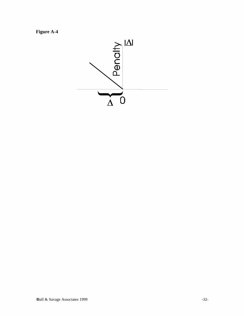
Mean Loss and other adaptations of MADA simple but useful adaptation of MAD, used in EPPO.xls, is Mean Loss, in which ∆ measures only thedeviation below 0 (not below the mean), as shown in Figure A-4. The mean loss of the three examplesabove is shown in Table A-2, clearly indicating that B is the least risky.

Mean loss is the average of one’s losses. That is if you have a 50% chance of winning $1 or losing $1 themean loss is 50¢. Mean loss has the desirable feature of distinguishing between upside and downside risk.However, like MAD it is a linear loss measure. That is, if you had a million dollars, and started losingmoney, mean loss would impose the same penalty on losing your 1st dollar that it does on losing your lastdollar.

It is more realistic for the penalty to increase with deviation, as it does in the case of variance. The MADmodel may be adapted further to model any piece-wise linear convex penalty F(∆) such as that displayedin Figure A-5. Note that any number of straight-line penalty slopes and even a constraint on ∆ may beimposed.

To create an LP model of this risk function, define two new LP variables for each scenario as follows, y1j ≥0 and y2j ≥ 0. These variables are constrained as shown in Equations 4, 5, 6, and 7.

y1j ≥ -∆j-c Equation 4

y1j ≤ d-c Equation 5

y2j ≥ -∆j-d Equation 6

y2j< e-d Equation 7

For each scenario define Fj as in Equation 8.

F j = a y1j + b y2j Equation 8

Then the overall objective of the LP is to minimize the function defined in Equation 9.

1

1M jj

M

F=

∑ Equation 9

In this way, customized risk measures may be constructed. One could even create a piece-wise linearapproximation of the variance or semi-variance (squared deviation below the mean) if desired.

A customized risk measure suitable for production projects can easily be developed from the paradigmsuggested in Figure A-5. In production projects, the danger is not so much an outright loss as it is anerosion of value. A risk parameter which measured Mean Value Erosion would simply involve setting “c” inFigure A-5 at a point above zero equal to the required economic threshold.


Appendix B: Notation and Algebraic Representation of EPPO

The Model

Table B-1 shows the notation used in EPPO.XLS model, while Table B-2 shows the model flow.

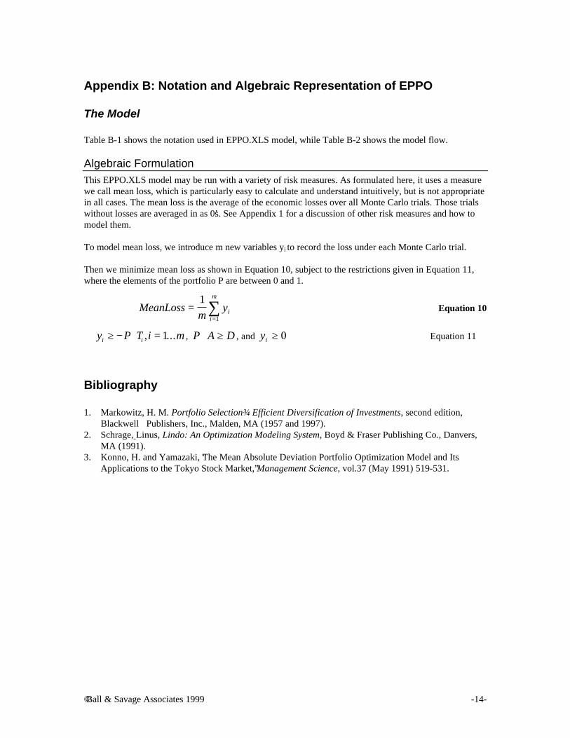
Algebraic FormulationThis EPPO.XLS model may be run with a variety of risk measures. As formulated here, it uses a measurewe call mean loss, which is particularly easy to calculate and understand intuitively, but is not appropriatein all cases. The mean loss is the average of the economic losses over all Monte Carlo trials. Those trialswithout losses are averaged in as 0’s. See Appendix 1 for a discussion of other risk measures and how tomodel them.

To model mean loss, we introduce m new variables yi to record the loss under each Monte Carlo trial.

Then we minimize mean loss as shown in Equation 10, subject to the restrictions given in Equation 11,where the elements of the portfolio P are between 0 and 1.

MeanLossm

yii

m

==∑1

1

Equation 10

y P T i mi i≥ − ⋅ =, ...1 , P A D⋅ ≥ , and yi ≥ 0 Equation 11

Bibliography

1. Markowitz, H. M. Portfolio SelectionEfficient Diversification of Investments, second edition,Blackwell Publishers, Inc., Malden, MA (1957 and 1997).

2. Schrage, Linus, Lindo: An Optimization Modeling System, Boyd & Fraser Publishing Co., Danvers,MA (1991).

3. Konno, H. and Yamazaki, “The Mean Absolute Deviation Portfolio Optimization Model and ItsApplications to the Tokyo Stock Market,” Management Science, vol.37 (May 1991) 519-531.


TablesTable 1

Outcome NPV$MM

IndependentProbability

Safe Dry Hole -10 40%

Success 50 60%

Risky Dry Hole -10 60%

Success 80 40%

Table 2

Outcomes of Investing 50% in Each ProjectWith Statistical Independence

Safe Risky Probability Return in $MM Result1 Success Success 60% x 40%

=24%50% x $50 + 50% x $80 = $65 Keep Job

2 Success Dry Hole 60% x 60%=36%

50% x $50 + 50% x (-$10) = $20 Keep Job

3 Dry Hole Success 40% x 40%=16%

50% x (-$10) + 50% x $80 = $35 Keep Job

4 Dry Hole Dry Hole 40% x 60%=24%

50% x (-$10) + 50% x (-$10) = (-$10) Lose Job

ENPV24% x $65 + 36% x $20 + 16% x $35 + 24% x (-$10) = $26


Table 3

Stock Portfolios E&P Projects

Types of Uncertaintiesa. Stock portfolio models are primarily based on

price uncertainty.

E&P projects face both local uncertaintiesinvolving the discovery and production of oil at agiven site, and global uncertainties involvingprices, politics etc.

b. The uncertainties of future stock returns are

generally symmetric and bell shaped.

Distribution of a Stock ReturnMean Return = 2

00.05

0.10.15

0.20.25

0.30.35

0.40.45

-2 0 2 4 6 8

Return

Rel

ativ

e L

iklih

oo

d

c. Estimates of distributions and statisticaldependence are based at least in part on pasthistory

The economic uncertainties of E&P are anythingbut normal.

Distribution of an E&P Project ReturnMean Return = 2

0

0.05

0.1

0.15

0.2

0.25

0.3

0.35

0.4

0.45

-2 0 2 4 6 8

Return

Rel

ativ

e L

ikel

iho

od

Distributions and statistical dependence of priceinformation may be based on history. Otheruncertainties must be modeled through decisiontrees or simulation.

Risk Measures

Dry Hole EconomicSuccess


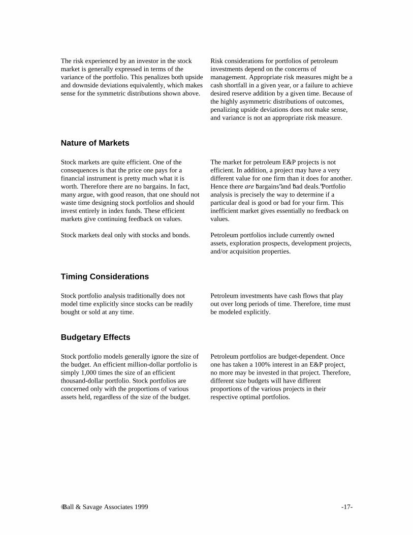
The risk experienced by an investor in the stockmarket is generally expressed in terms of thevariance of the portfolio. This penalizes both upsideand downside deviations equivalently, which makessense for the symmetric distributions shown above.

Risk considerations for portfolios of petroleuminvestments depend on the concerns ofmanagement. Appropriate risk measures might be acash shortfall in a given year, or a failure to achievedesired reserve addition by a given time. Because ofthe highly asymmetric distributions of outcomes,penalizing upside deviations does not make sense,and variance is not an appropriate risk measure.

Nature of Markets

Stock markets are quite efficient. One of theconsequences is that the price one pays for afinancial instrument is pretty much what it isworth. Therefore there are no bargains. In fact,many argue, with good reason, that one should notwaste time designing stock portfolios and shouldinvest entirely in index funds. These efficientmarkets give continuing feedback on values.

The market for petroleum E&P projects is notefficient. In addition, a project may have a verydifferent value for one firm than it does for another.Hence there are “bargains” and “bad deals.” Portfolioanalysis is precisely the way to determine if aparticular deal is good or bad for your firm. Thisinefficient market gives essentially no feedback onvalues.

Stock markets deal only with stocks and bonds. Petroleum portfolios include currently ownedassets, exploration prospects, development projects,and/or acquisition properties.

Timing Considerations

Stock portfolio analysis traditionally does notmodel time explicitly since stocks can be readilybought or sold at any time.

Petroleum investments have cash flows that playout over long periods of time. Therefore, time mustbe modeled explicitly.

Budgetary Effects

Stock portfolio models generally ignore the size ofthe budget. An efficient million-dollar portfolio issimply 1,000 times the size of an efficientthousand-dollar portfolio. Stock portfolios areconcerned only with the proportions of variousassets held, regardless of the size of the budget.

Petroleum portfolios are budget-dependent. Onceone has taken a 100% interest in an E&P project,no more may be invested in that project. Therefore,different size budgets will have differentproportions of the various projects in theirrespective optimal portfolios.


Table 4

Current Practice Asset Interplay Management

1. Selecting a set of E&P projects to fundRank (high-grade) the projects, start at the top ofthe list and go down until the budget is exceeded.

Select the set of projects that achieve optimal trade-offs of various risks and economic factors.

2. Determining long-term vs. short-term goalsEstablish long-term “return on investment”11 andgrowth goals independent of their implications forthe concomitant long-term risk or short-termvolatility.

Make informed trade-offs between long-term goalsfor growth and the risks of short-term volatility,failure to meet reserve requirements or othermeasures of risk.12

3. Dealing with political and environmental riskPolitical and environmental risks areconsidered subjectively on a project byproject basis.

Political and environmental risk of the entireportfolio is managed by taking the interplay amongprojects into account.

4. Evaluating a project for purchase or saleDetermine the project’s “market” value, that is, whatother firms might pay for it, or base its value on anestimate of its ENPV.

Determine what the project is worth in the contextof the firm’s current holdings. Remember, I wouldn’tspend a dime on a policy to insure your house, butan identical policy on my house is valuable to me,even though it has a negative NPV.

5. Determining the risk related cost of constraints and policiesThe costs of company policies and externalconstraints are appraised subjectively.

The implications of constraints andcompany policies can be evaluated on arisk/return basis.13

11 Or return on capital employed, or similar metric.12 It is important to note that this approach captures the insights underlying utility theory, preferencecurves, etc., while avoiding the practical difficulties that arise from their explicit application. See Kenyon,Savage, and Ball [28].

13 Constraints often reflect “strategic” issues of concern to top management, e.g., reserves replacement, cashflow for debt repayment, etc. Relative to stock market valuation, these may at times be as important ormore important than ENPV. However, these constraints can be incorporated into the portfolio analysisand evaluated for their effects on risk and return. Brashear [25]


6. Determining Strategic Criteria for Future ExplorationMissing ingredients or strategic weaknessesare difficult to identify.

Missing ingredients or strategic thrusts thatwould contribute to the robustness of theportfolio are identified. The result is ashopping list of desirable qualities foradditional projects or programs, given yourfirm’s current portfolio and situation.14

7. Increasing the Value of the Firm

Sole focus is on expected net present value. The focus of real E&P companies is neversolely on expected net present value, butincludes reserves replacement, debt ratios,cash flows, etc. At one extreme, risk isalmost entirely ignored, but Froot,Scharfstein and Stein contend [27] thatthere are situations in which risk reductioncan increase the value of the firm byassuring that cash flow is available whenneeded for critical investment.

Table A-1

Project Outcome NPV$MM

Probability Mean Variance

A Failure -10 50% -10*.5+30*.5=10 .5*(-10-10)2+.5*(30-10)2=400

Success 30 50%

B Failure 0 80% 0*.8+50*.2=10 .8*(0-10)2+.2*(50-10)2=400

Success 50 20%

C Failure -30 20% -30*.2+20*.8=10 .2*(-30-10)2+.8*(20-10)2=400

Success 20 80%

14 “Current holdings,” of course, represents, the mass of most portfolios. “Hold and produce” takes little or nocapital, requires no overt decisions, and yields great returns, especially if opportunity costs are ignored.However, serious consideration of the trading of current holdings (i.e., the sale of current assets inexchange for the purchase of new ones) is usually not seriously considered in any systemic way. However,such a study could significantly enhance the efficient frontier. In any event, a crucial point is that bothcurrent holdings and new projects opportunities must be evaluated together, as the portfolio’s risk dependson the ways in which all of its constituent parts interact. Brashear [25]


Table A-2

Project Outcome NPV$MM

Probability Mean Loss

A Failure -10 50% 10*.5 + 0*.5 = 5

Success 30 50%

B Failure 0 80% 0*.8 + 0*.2=0

Success 50 20%

C Failure -30 20% 30*.2 + 0 *.8=6

Success 20 80%

Table B-1

Notationn -

m-

P -

Ti -

A -

NPVi(P) -

R(P) -

D-

Number of projects under consideration (5 in our example)

Number of Monte Carlo trials (40 in our example)

The portfolio. This is a vector of length n consisting of the working interest(between 0 and 100%) in each project. EPPO assumes that any workinginterest is possible, however, the model may be modified to force an “all ornothing” policy, or some other minimum or maximum working interest.

The ith in the sequence of Monte Carlo Trials modeling the joint uncertainNPV’s of the projects. Ti is a vector of length n.

The average NPV of each project over the m trials, a vector of length n.

The NPV of portfolio P under Monte Carlo trial i.

A risk measure associated with portfolio P, calculated from NPVi(P), i=1..m.In EPPO, R(P) is the Mean Loss of P.

A desired level of ENPV


Table B-2

Model Flow

Monte CarloSimulation

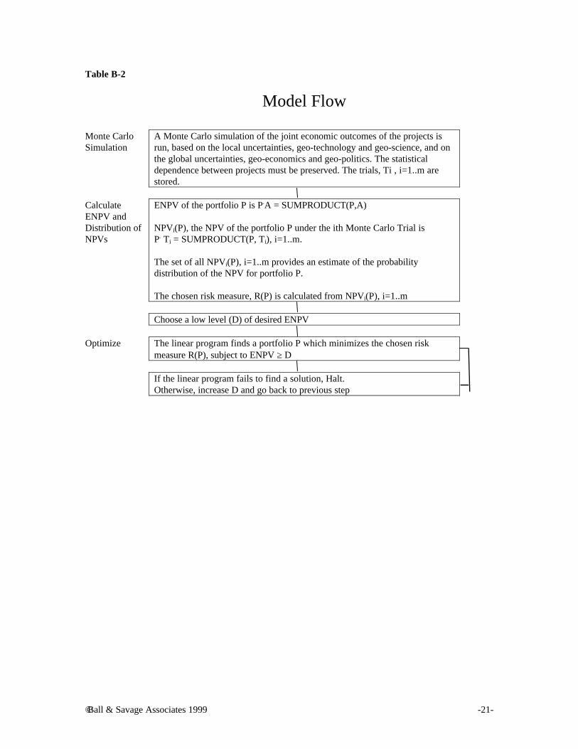
A Monte Carlo simulation of the joint economic outcomes of the projects isrun, based on the local uncertainties, geo-technology and geo-science, and onthe global uncertainties, geo-economics and geo-politics. The statisticaldependence between projects must be preserved. The trials, Ti , i=1..m arestored.

CalculateENPV andDistribution ofNPVs

ENPV of the portfolio P is P.A = SUMPRODUCT(P,A)

NPVi(P), the NPV of the portfolio P under the ith Monte Carlo Trial isP. Ti = SUMPRODUCT(P, Ti), i=1..m.

The set of all NPVi(P), i=1..m provides an estimate of the probabilitydistribution of the NPV for portfolio P.

The chosen risk measure, R(P) is calculated from NPVi(P), i=1..m

Choose a low level (D) of desired ENPV

Optimize The linear program finds a portfolio P which minimizes the chosen riskmeasure R(P), subject to ENPV ≥ D

If the linear program fails to find a solution, Halt.Otherwise, increase D and go back to previous step


Figures

Figure 1 a and b

Distribution of Outcomes of “Safe”Project

0.00

0.10

0.20

0.30

0.40

0.50

0.60

0.70

0.80

0.90

1.00

-15

-10 -5 0 5

10 15 20 25 30 35 40 45 50 55 60 65 70 75 80 85

Return

Pro

bab

ility

Distribution of Outcomes of “Risky”Project

0.00

0.10

0.20

0.30

0.40

0.50

0.60

0.70

0.80

0.90

1.00

-15

-10

-5 0 5 10 15 20 25 30 35 40 45 50 55 60 65 70 75 80 85

Return

Probability

Figure 2

0.00

0.10

0.20

0.30

0.40

0.50

0.60

0.70

0.80

0.90

1.00

-15

-10 -5 0 5 10 15 20 25 30 35 40 45 50 55 60 65 70 75 80 85

Return

Pro

bab

ility

ENPV$26 MM

ENPV$26 MM

ENPV Still 26MM

Chance of Losing Job 24%

Distribution of Outcomes of 50/50 Split


Figure 3 a, b, c, and d

Projects with similar cash flow profiles will bepositively correlated over time.

Projects with dissimilar cash flow profilesmay be negatively correlated over time.

A portfolio consisting of a 50% share in each of theabove cash flows (shown in solid line below) resultsin wide swings from negative to positive cash flow.

A portfolio consisting of a 50% share in each of theabove cash flows (shown in solid line below) resultsin a relatively smoother cash flow.

Figure 4

00.10.20.30.40.50.60.70.80.9

1

24 26 28 30

Expected Return

Ris

k

Cash flow of combinedprojects shown as solid line

1 2 3 4 5 6 7 8 9 10 11 12 13 14 15 16

Years

1 2 3 4 5 6 7 8 9 10 11 12 13 14 15 16

Years

-6

-4

-2

0

2

4

6

8

1 2 3 4 5 6 7 8 9 10 11 12 13 14 15 16

Years

Cas

h F

low

-6

-4

-2

0

2

4

6

8

1 2 3 4 5 6 7 8 9 10 11 12 13 14 15 16

Years

Mix of Safeand Risky

Safe

Risky


Figure 5

00.10.20.30.40.50.60.70.80.9

1

24 26 28 30

Expected Return

Ris

k

Figure 6

00.10.20.30.40.50.60.70.80.9

1

24 26 28 30

Expected Return

Ris

k EfficientFrontier


Figure 7

EPPO.XLSInputs1. Monte Carlo trials of the economic outcomes of

five projects designed to preserve the statisticaldependence among projects. The user mustprovide this data for the projects underconsideration.

2. Required ENPV3. Budget.

Outputs4. The Portfolio: percentages of each project

undertaken, optimized to minimize the MeanLoss (5) for required ENPV (2) and Budget (3).

5. Mean Loss of portfolio.6. Distribution of outputs for this portfolio.7. Pie chart of % of budget in the various projects.

E&P PortfolioOptimizer EPPO© Copyright 1998, Ball & Savage Assoc.

Portfolio StatisticsNPV Loss

Exp. $2,500 $127>=

Req. $2,500

Cost ReservesExp. $791 484

<=

Req. $1,100

Portfolio 30% 0% 41% 100% 41%Project Statistics Project A Project B Project C Project D Project E

Exp. NPV $820.39 $170.80 $890.51 $1,255.16 $1,562.84

Exp. Cost $372.69 $47.05 $374.08 $370.07 $383.88 $1,547.77

Exp. Reserves 161 32 218 240 262

Monte Carlo Generated Data Optimization CalculationsPortfolio by $127

Project A Project B Project C Project D Project E Scenario PenaltyTrial 1 872.95$ (8.00)$ (100.00)$ (300.00)$ 23,147.60$ $9,315 ($9,315) $0 $0Trial 2 1,944.41$ (47.00)$ (100.00)$ (250.00)$ (350.00)$ $142 ($142) $0 $0Trial 3 1,910.78$ (47.00)$ (300.00)$ 6,264.29$ (350.00)$ $6,564 ($6,564) $0 $0

: : : : : : : : : :: : : : : : : : : :

Trial 40 (393.00)$ (47.00)$ 1,441.28$ (300.00)$ (350.00)$ $36 ($36) $0 $0

0%

10%

20%

30%

40%

50%

60%

70%

($1,

073)

3309

.67

$7,6

92

$12,

075

$16,

457

$20,

840

$25,

222

A

B

C

D

E

Mean Losscalculations


Figure 8a

X Z

Y


Figure 8b


Figure 8c


Figure A-1


Figure A-2 a, b, and c

Project A

0

0.1

0.2

0.3

0.4

0.5

-30

-20

-10 0 10 20 30 40 50

Return

Pro

bab

ility

Project B

0

0.1

0.2

0.3

0.4

0.5

0.6

0.7

0.8

-30

-20

-10 0 10 20 30 40 50

Return

Pro

bab

ility

Project C

0

0.1

0.2

0.3

0.4

0.5

0.6

0.7

0.8

-30

-20

-10 0 10 20 30 40 50

Return

Pro

bab

ility


Figure A-3


Figure A-4


Figure A-5

Documents

Notes on Exploration and Production Portfolio Optimization