Embed Size (px)
Citation preview

Notes for MATH 383 — Height Functions in Number Theory(Winter 2018)
SIYAN DANIEL LI
These are live-TEX’d notes for a course taught at the University of Chicago in Winter 2018 by ProfessorKazuya Kato. Any errors are attributed to the note-taker. If you find any such errors or have comments atlarge, don’t hesitate to contact said note-taker at [email protected].
1 January 3, 2018
The subject of this course consists of Diophantine geometry and heights of numbers, or in other words,height functions in number theory. The course outline is as follows:
§1 A theorem of Siegel (a special case of §2) and the ABC conjecture. Mochizuki has put a proof of thelatter on his webpage, but it’s really hard to understand, and the situation surrounding the proof is verydifficult.
§2 Results and conjectures in Diophantine geometry, especially finiteness results and conjectures.
§3 The Vojta conjectures, for which heights in number fields are important.
§4 Nevanlinna analogues of the above, for which heights of holomorphic functions are important. This isrelated to §2 and §3 by analogy.
§5 The proof of the Mordell conjecture by Faltings, the Tate conjecture for abelian varieties by Faltings, andthe Tate conjecture for algebraic cycles, assuming the finitude of the number of motives with boundedheights, by Koshikawa (one of my students!).
Here are some good textbooks:
1. Fundamentals of Diophantine Geometry (which is the study of algebraic arithmetic geometry concerningrational points and integral points of algebraic equations) by Lang.
Diophantine geometry is named after an ancient Greek mathematician who studied rational and integralpoints of algebraic equations. Fermat and many others have also studied such questions.
Let us start with §1. We now introduce a theorem of Siegel and later the ABC conjecture.
1.1 Theorem (Siegel). Let A ⊇ Z be an integral domain that is finitely generated over Z. Then
(x, y) ∈ A× ×A× | x+ y = 1
is a finite set.
1.2 Examples.
1
MATH 383 — Height Functions in Number Theory Siyan Daniel Li
• Let A = Z[12 ]. Then the corresponding set is just (2,−1), (−1, 2), (1
2 ,12), which can be shown by
any high school student.
• Let A = Z[16 ]. Then the corresponding set consists of (2,−1), (3,−2), (9,−8), (4,−3) and other
pairs obtained from elementary operations (such as x + y = 1 =⇒ 1x −
yx = 1, but I shall not
explicitly define these operations here), though I do not know how to prove this elementarily.
We include the ABC conjecture in this section because it implies Siegel’s theorem, demonstrating thatthe two subjects are indeed related. The ABC conjecture was originally formulated by Osterle and Masserin 1985, and its original form proceeds as follows:
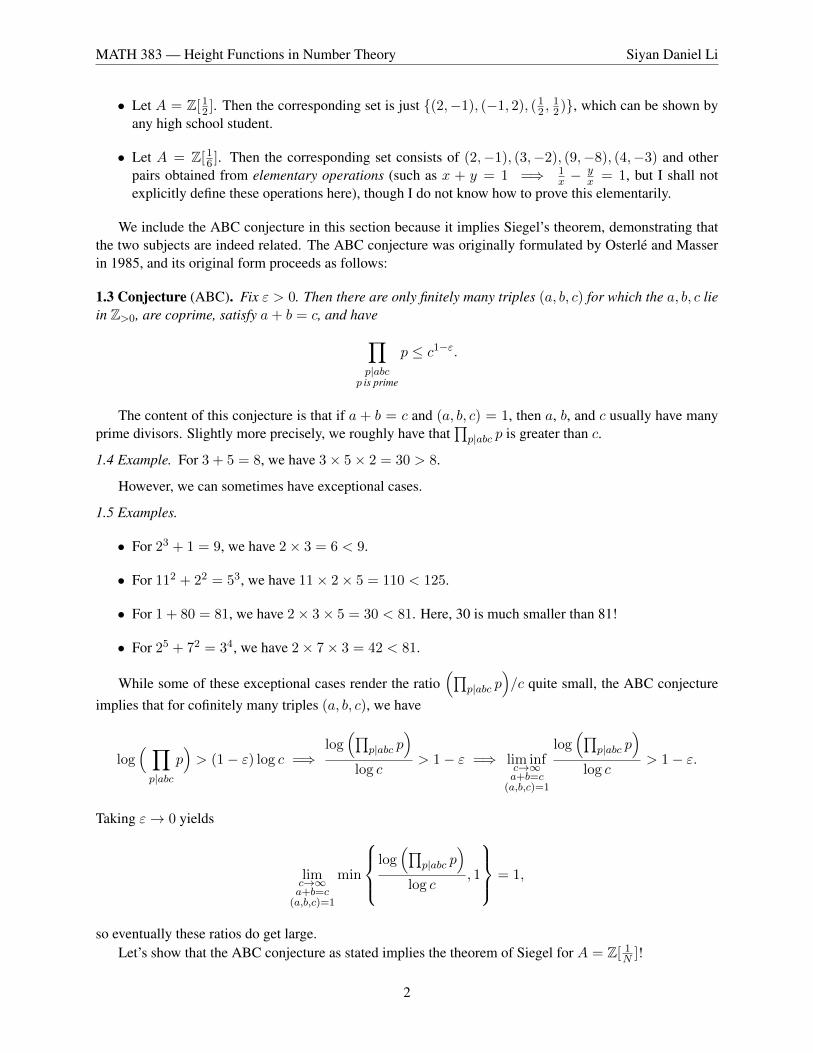
1.3 Conjecture (ABC). Fix ε > 0. Then there are only finitely many triples (a, b, c) for which the a, b, c liein Z>0, are coprime, satisfy a+ b = c, and have∏
p|abcp is prime
p ≤ c1−ε.
The content of this conjecture is that if a + b = c and (a, b, c) = 1, then a, b, and c usually have manyprime divisors. Slightly more precisely, we roughly have that
∏p|abc p is greater than c.
1.4 Example. For 3 + 5 = 8, we have 3× 5× 2 = 30 > 8.
However, we can sometimes have exceptional cases.
1.5 Examples.
• For 23 + 1 = 9, we have 2× 3 = 6 < 9.
• For 112 + 22 = 53, we have 11× 2× 5 = 110 < 125.
• For 1 + 80 = 81, we have 2× 3× 5 = 30 < 81. Here, 30 is much smaller than 81!
• For 25 + 72 = 34, we have 2× 7× 3 = 42 < 81.
While some of these exceptional cases render the ratio(∏
p|abc p)/c quite small, the ABC conjecture
implies that for cofinitely many triples (a, b, c), we have
log( ∏p|abc
p)> (1− ε) log c =⇒
log(∏
p|abc p)
log c> 1− ε =⇒ lim inf
c→∞a+b=c
(a,b,c)=1
log(∏
p|abc p)
log c> 1− ε.
Taking ε→ 0 yields
limc→∞a+b=c
(a,b,c)=1
min
log(∏
p|abc p)
log c, 1
= 1,
so eventually these ratios do get large.Let’s show that the ABC conjecture as stated implies the theorem of Siegel for A = Z[ 1
N ]!
2

MATH 383 — Height Functions in Number Theory Siyan Daniel Li
Proof of Siegel’s theorem using ABC. Let (x, y) lie in the desired subset. Then x + y = 1, and pulling outdenominators and rearranging if necessary yields an equation a + b = c, where the a, b, and c are positiveintegers satisfying (a, b, c) = 1. Since x and y are units in Z[ 1
N ], they only have nonzero p-adic valuationfor p dividing N . As the a, b, and c are the result of clearing denominators from x and y, we see that theprimes dividing abc also divide N . Therefore
N ≥∏p|abc
p ≥ c1−ε
for cofinitely many (a, b, c) as above. Thus the options for c are bounded, so there are finitely many alto-gether.
How would we formulate ABC for more general rings A? We’ll discuss one perspective this next time.
2 January 5, 2018
One can almost deduce Fermat’s last theorem from the ABC conjecture. Namely, ABC implies that
(x, y, z, n) | x, y, z ∈ Z r 0, n ≥ 4 ∈ Z, xn + yn = zn, (x, y, z) = 1
is finite. Of course, the actual Fermat’s last theorem says that this set is empty. Furthermore, the Mordellconjecture (proved by Faltings) says that the above set is finite when you fix the value of n, because xn +yn = zn cuts out a projective curve in P2 of genus (n − 1)(n − 2)/2, which is at least 2 when n ≥ 4, andthe Q-rational points of this curve correspond to solutions in the above set.
All the theorems we’ve just quoted are really strong. We’ve seen some of that already, and as furtherevidence, the ABC conjecture implies the following stronger version of the last paragraph:
2.1 Conjecture (Fermat–Catalan). The set(a, b, c) ∈ Z3
>0a+ b = c, gcda, b, c = 1, and there exists x, y, z ∈ Z and m,n, k ∈ Z>0
such that a = xm, b = yn, c = zk, and 1m + 1
n + 1k < 1.
is finite.
Proof of the Fermat–Catalan conjecture using ABC. Because a, b, and c have the same prime divisors as x,y, and z (respectively), we have∏
p|abc
p ≤ xyz ≤ zk/mzk/nz = zk( 1m
+ 1n
+ 1k
) = c( 1m
+ 1n
+ 1k
).
By choosing a sufficiently small ε, we see that this is bounded above by c1−ε for all choices of (m,n, k),and the ABC conjecture tells us that there are only finitely many such (a, b, c) for which (a, b, c) = 1.
The Fermat–Catalan conjecture is an amalgamation of Fermat’s last theorem and the following result.
2.2 Theorem (Catalan conjecture). The only solution to xm − yn = 1, for m, n ≥ 2 and positive integersx and y, is 32 − 23 = 1.
Even though the ABC conjecture implies the generalized finitude that the Fermat–Catalan conjecturebrings, it doesn’t seem to give the precise, concrete description that the Catalan conjecture provides. TheCatalan conjecture was proved by Mihailescu in 2002, and it was a big deal.
We will now discuss a connection with P1 r 0, 1,∞, which leads to a geometric generalization of ourABC discussion (and of our Diophantine approximation business at large). First, let O(C) denote the set ofholomorphic functions C−→C, and let us discuss a strange fundamental philosophy:
3
MATH 383 — Height Functions in Number Theory Siyan Daniel Li
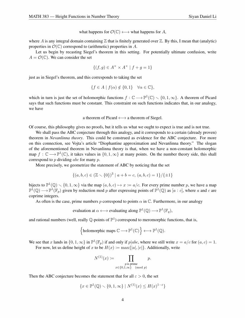
what happens for O(C)←→ what happens for A,
where A is any integral domain containing Z that is finitely generated over Z. By this, I mean that (analytic)properties in O(C) correspond to (arithmetic) properties in A.
Let us begin by recasting Siegel’s theorem in this setting. For potentially ultimate confusion, writeA = O(C). We can consider the set
(f, g) ∈ A× ×A× | f + g = 1
just as in Siegel’s theorem, and this corresponds to taking the set
f ∈ A | f(α) /∈ 0, 1 ∀α ∈ C,
which in turn is just the set of holomorphic functions f : C−→P1(C) r 0, 1,∞. A theorem of Picardsays that such functions must be constant. This constraint on such functions indicates that, in our analogy,we have
a theorem of Picard←→ a theorem of Siegel.
Of course, this philosophy gives no proofs, but it tells us what we ought to expect is true and is not true.We shall pass the ABC conjecture through this analogy, and it corresponds to a certain (already proven)
theorem in Nevanlinna theory. This could be construed as evidence for the ABC conjecture. For moreon this connection, see Vojta’s article “Diophantine approximation and Nevanlinna theory.” The sloganof the aforementioned theorem in Nevanlinna theory is that, when we have a non-constant holomorphicmap f : C−→P1(C), it takes values in 0, 1,∞ at many points. On the number theory side, this shallcorrespond to p dividing abc for many p.
More precisely, we geometrize the statement of ABC by noticing that the set
(a, b, c) ∈ (Z r 0)3 | a+ b = c, (a, b, c) = 1/±1
bijects to P1(Q) r 0, 1,∞ via the map (a, b, c) 7→ x := a/c. For every prime number p, we have a mapP1(Q)−→P1(Fp) given by reduction mod p after expressing points of P1(Q) as [a : c], where a and c arecoprime integers.
As often is the case, prime numbers p correspond to points α in C. Furthermore, in our analogy
evaluation at α←→ evaluating along P1(Q)−→P1(Fq),
and rational numbers (well, really Q-points of P1) correspond to meromorphic functions, that is,holomorphic maps C−→P1(C)
←→ P1(Q).
We see that x lands in 0, 1,∞ in P1(Fp) if and only if p|abc, where we still write x = a/c for (a, c) = 1.For now, let us define height of x to be H(x) := max|a|, |c|. Additionally, write
N (1)(x) :=∏
p is primex∈0,1,∞ (mod p)
p.
Then the ABC conjecture becomes the statement that for all ε > 0, the set
x ∈ P1(Q) r 0, 1,∞ | N (1)(x) ≤ H(x)1−ε
4

MATH 383 — Height Functions in Number Theory Siyan Daniel Li
is finite. Given that, for any fixed C > 0, the set
x ∈ P1(Q) | H(x) ≤ C
is also finite1, we see that the ABC conjecture in this light implies that
x ∈ P1(Q) r 0, 1,∞ | N (1)(x) ≤ C
is finite. From this, one can deduce Siegel’s theorem.The ABC conjecture says that we roughly have N (1)(x) ≥ H(x). The corresponding Nevanlinna
statement is that we roughly have N (1)(α) ≥ Tf (α), and this latter statement is known to be true.2
In this geometric optic, we can replace P1r0, 1,∞with more general algebraic varieties over numberfields. Let F be a number field, and let X be an algebraic variety3 over F . Let X be a compactification ofX over F , and here now X rX takes the role of 0, 1,∞. We can consider both the C-points as well asF -points of these varieties, and this is the setting in which Vojta formulates his conjectures.
3 January 8, 2018
Recall from Lecture 1 that the ABC conjecture implies Siegel’s theorem for Z[ 1N ]. This time, let me begin
by saying a few words on the work of Mochizuki. We have a map
P1(Q) r 0, 1,∞−→elliptic curves over Q/∼λ 7−→ Eλ : y2 = x(x− 1)(x− λ).
And roughly speaking, for any prime number p,
λ ∈ 0, 1,∞ (mod p) ⇐⇒ Eλ has bad reduction at p.
The reason for this is that the equation defining Eλ becomes singular modulo p precisely when λ becomes0, 1, or∞ modulo p.
Define the height of Eλ to be H(Eλ) := H(λ), and recall that the latter height is defined to bemax|a|, |c|, where λ = a/c for coprime a and c. Now Mochizuki was Faltings’s student, the latterof whom defined the heights of abelian varieties over number fields (and used them to prove the Mordellconjecture!).
Last time, we saw that the ABC conjecture corresponds to saying we roughly have∏p is prime
λ∈0,1,∞ (mod p)
p ≥ H(λ)
which hence corresponds to saying that we roughly have∏p is prime
Eλ has bad reduction at p
p ≥ H(Eλ),
which ties our story of the ABC conjecture to the story of elliptic curves.Around the 2000s, Mochizuki was studying something more understandable, which was Hodge–Arakelov
theory (a form of “p-adic Hodge theory” for elliptic curves over number fields). He wanted to tackle the ABCconjecture using the above elliptic curve strategy. The strategy is to extract information from πet
1 (E r 0),which is related to his previous work from the 1990s on Grothendieck’s conjecture:
1See Proposition 9.4.2For the definitions of N (1)(α) and Tf (α), see Lecture 17.3For me, all algebraic varieties are assumed to be geometrically irreducible.
5
MATH 383 — Height Functions in Number Theory Siyan Daniel Li
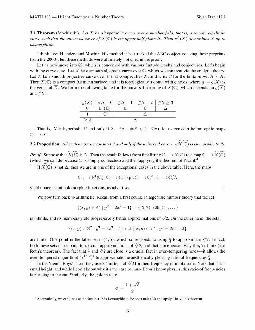
3.1 Theorem (Mochizuki). Let X be a hyperbolic curve over a number field, that is, a smooth algebraiccurve such that the universal cover of X(C) is the upper half plane ∆. Then πet
1 (X) determines X up toisomorphism.
I think I could understand Mochizuki’s method if he attacked the ABC conjecture using these preprintsfrom the 2000s, but these methods were ultimately not used in his proof.
Let us now move into §2, which is concerned with various finitude results and conjectures. Let’s beginwith the curve case. Let X be a smooth algebraic curve over C, which we can treat via the analytic theory.Let X be a smooth projective curve over C that compactifies X , and write S for the finite subset X r X .Then X(C) is a compact Riemann surface, and it is topologically a donut with g holes, where g := g(X) isthe genus of X . We form the following table for the universal covering of X(C), which depends on g(X)and #S:
g(X) #S = 0 #S = 1 #S = 2 #S ≥ 3
0 P1(C) C C ∆
1 C ∆
≥ 2 ∆
That is, X is hyperbolic if and only if 2 − 2g − #S < 0. Next, let us consider holomorphic mapsC−→X .
3.2 Proposition. All such maps are constant if and only if the universal covering X(C) is isomorphic to ∆.
Proof. Suppose that X(C) is ∆. Then the result follows from first lifting C−→X(C) to a map C−→ X(C)(which we can do because C is simply connected) and then applying the theorem of Picard.4
If X(C) is not ∆, then we are in one of the exceptional cases in the above table. Here, the maps
C −→ P1(C), C−→C, exp : C−→C×, C−→C/Λ
yield nonconstant holomorphic functions, as advertised.
We now turn back to arithmetic. Recall from a first course in algebraic number theory that the set
(x, y) ∈ Z2 | y2 = 2x2 − 1 = (5, 7), (29, 41), . . .
is infinite, and its members yield progressively better approximations of√
2. On the other hand, the sets
(x, y) ∈ Z2 | y3 = 2x3 − 1 and (x, y) ∈ Z2 | y3 = 2x3 − 3
are finite. One point in the latter set is (4, 5), which corresponds to using 54 to approximate 3
√2. In fact,
both these sets correspond to rational approximations of 3√
2, and that’s one reason why they’re finite (useRoth’s theorem). The fact that 5
4 and 3√
2 are close is a crucial fact in even-tempering notes—it allows theeven-tempered major third (21/12)4 to approximate the aesthetically pleasing ratio of frequencies 5
4 .In the Vienna Boys’ choir, they use 5:4 instead of 3
√2 for their frequency ratio of do:mi. Note that 5
4 hassmall height, and while I don’t know why it’s the case because I don’t know physics, this ratio of frequenciesis pleasing to the ear. Similarly, the golden ratio
φ :=1 +√
5
2
4Alternatively, we can just use the fact that ∆ is isomorphic to the open unit disk and apply Liouville’s theorem.
6
MATH 383 — Height Functions in Number Theory Siyan Daniel Li
also has small height (we haven’t defined heights of arbitrary algebraic numbers yet, but we can5), and thisquantity is known to be beautiful for the eyes. The moral of the story is that algebraic numbers of smallheight are aesthetically pleasing.
Returning to pure mathematics, let us introduce the Mordell conjecture, which is a theorem of Faltings:
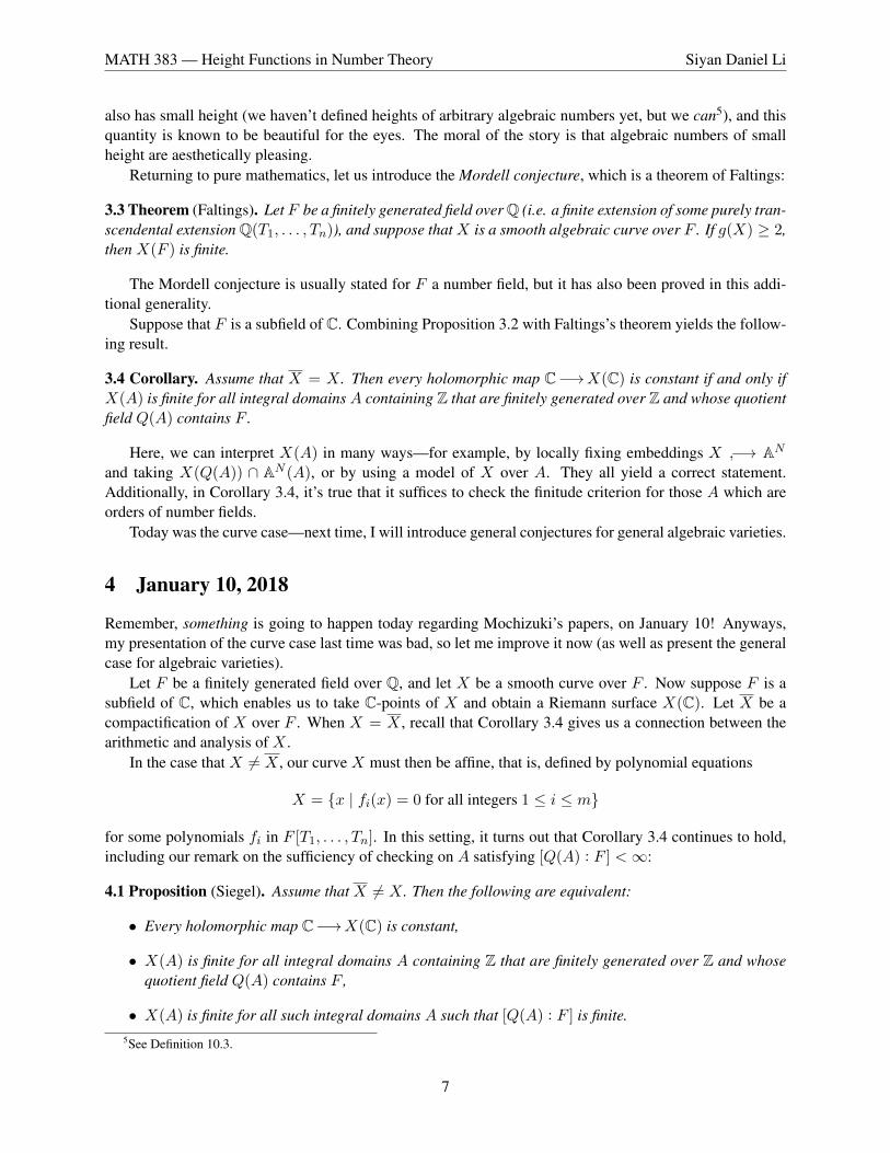
3.3 Theorem (Faltings). Let F be a finitely generated field over Q (i.e. a finite extension of some purely tran-scendental extension Q(T1, . . . , Tn)), and suppose thatX is a smooth algebraic curve over F . If g(X) ≥ 2,then X(F ) is finite.
The Mordell conjecture is usually stated for F a number field, but it has also been proved in this addi-tional generality.
Suppose that F is a subfield of C. Combining Proposition 3.2 with Faltings’s theorem yields the follow-ing result.
3.4 Corollary. Assume that X = X . Then every holomorphic map C−→X(C) is constant if and only ifX(A) is finite for all integral domains A containing Z that are finitely generated over Z and whose quotientfield Q(A) contains F .
Here, we can interpret X(A) in many ways—for example, by locally fixing embeddings X −→ ANand taking X(Q(A)) ∩ AN (A), or by using a model of X over A. They all yield a correct statement.Additionally, in Corollary 3.4, it’s true that it suffices to check the finitude criterion for those A which areorders of number fields.
Today was the curve case—next time, I will introduce general conjectures for general algebraic varieties.
4 January 10, 2018
Remember, something is going to happen today regarding Mochizuki’s papers, on January 10! Anyways,my presentation of the curve case last time was bad, so let me improve it now (as well as present the generalcase for algebraic varieties).
Let F be a finitely generated field over Q, and let X be a smooth curve over F . Now suppose F is asubfield of C, which enables us to take C-points of X and obtain a Riemann surface X(C). Let X be acompactification of X over F . When X = X , recall that Corollary 3.4 gives us a connection between thearithmetic and analysis of X .
In the case that X 6= X , our curve X must then be affine, that is, defined by polynomial equations
X = x | fi(x) = 0 for all integers 1 ≤ i ≤ m
for some polynomials fi in F [T1, . . . , Tn]. In this setting, it turns out that Corollary 3.4 continues to hold,including our remark on the sufficiency of checking on A satisfying [Q(A) : F ] <∞:
4.1 Proposition (Siegel). Assume that X 6= X . Then the following are equivalent:
• Every holomorphic map C−→X(C) is constant,
• X(A) is finite for all integral domains A containing Z that are finitely generated over Z and whosequotient field Q(A) contains F ,
• X(A) is finite for all such integral domains A such that [Q(A) : F ] is finite.5See Definition 10.3.
7

MATH 383 — Height Functions in Number Theory Siyan Daniel Li
Before we explain what X(A) means, let us turn to the case of general algebraic varieties. They aregoverned by the conjectures of Lang and Vojta. Let X be an algebraic variety over F , which means that itcan be covered by finitely many affine algebraic varieties. First, consider the case where X itself is affine,which once again means that it is of the form
X = x | fi(x) = 0 for all integers 1 ≤ i ≤ m
for some polynomials fi in F [T1, . . . , Tn]. For any commutative ring A over F , we write
X(A) := x ∈ An | fi(x) = 0 for all integers 1 ≤ i ≤ m = HomF (O(X), A),
where O(X) := F [T1, . . . , Tn]/(f1, . . . , fm).For general algebraic varietiesX over F , consider an open coverX =
⋃rj=1 Uj ofX by affine algebraic
varieties Uj . Then, for any integral domain A over F satisfying the condition
A =⋂
m∈mSpec(A)
Am in Q(A),
we have the following description of the A-points of X:
X(A) = x ∈ X(Q(A)) | ∀m ∈ mSpec(A), ∃ an integer 1 ≤ j ≤ r such that x ∈ im(Uj(Am)−→X(Q(A)).
This also holds if we replace every instance of mSpec with Spec. In particular, we stress that X(A) doesnot simply equal
⋃ri=1 Ui(A).
4.2 Examples. Let us now examine some algebraic varieties.
• X = P1 r 0, 1 is affine and corresponds to the ring F [T, 1T ], which is isomorphic to
F [X,Y ]/(XY − 1) via X 7→ T, Y 7→ 1
T.
• X = P1 r 0, 1,∞ is affine and corresponds to the ring F [T, 1T ,
1T−1 ], which is isomorphic to
F [X1, X2, Y1, Y2]/(X1X2 − 1, Y1Y2 − 1, X1 − Y1 + 1) via X1 7→ T, X2 7→1
T, Y1 7→ T − 1, Y2 7→
1
T − 1.
Let us now travel to the analytic side. Let X be an algebraic variety over C, and write
A = Ohol(C) := holomorphic functions C−→C,X(A) := morphisms C−→X(C) of complex analytic spaces.
That is, X(A) is the set of holomorphic maps C−→X(C). More explicitly, when X is affine and cut outby polynomials f1, . . . , fm in C[T1, . . . , Tn], we have
X(A) = ϕ = (ϕ1, . . . , ϕn) ∈ Ohol(C)n | fi(ϕ) = 0 for all integers 1 ≤ i ≤ m.
For general algebraic varieties X over C, we can compute X(A) exactly as we did in the algebraic setting.Now Q(A) is the field of meromorphic functions C 99K C, the maximal ideals m of A are in bijection withpoints α in C, and under this correspondence we have
Am = Q(A) ∩ OholC,α,
where OholC,α is the stalk at α of the sheaf of holomorphic functions C−→C. Note that Ohol
C,α equals thesubring of convergent series in C[[T − α]], and Am equals the ring of meromorphic functions that are holo-morphic at α. In particular, if X =
⋃rj=1 Uj for some open affine algebraic subvarieties Uj , we once again
have X(A) 6=⋃rj=1 Uj(A) in general.
We now need a notion of hyperbolicity for general algebraic varieties over C.
8
MATH 383 — Height Functions in Number Theory Siyan Daniel Li
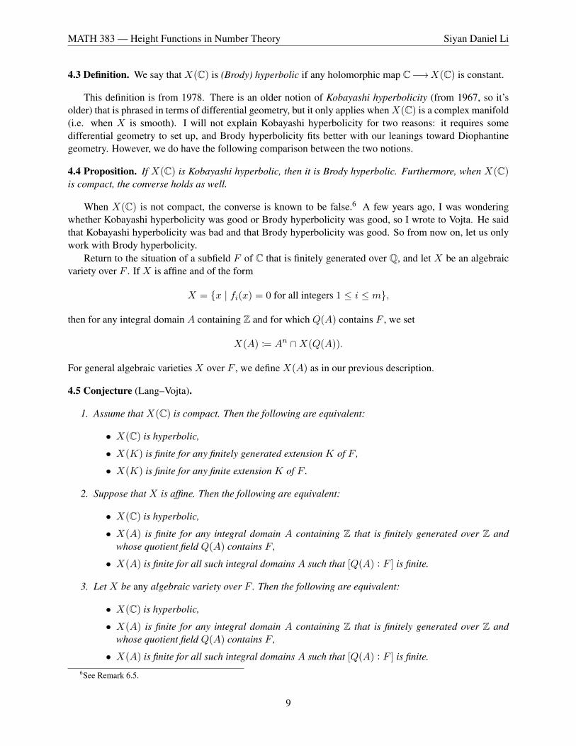
4.3 Definition. We say that X(C) is (Brody) hyperbolic if any holomorphic map C−→X(C) is constant.
This definition is from 1978. There is an older notion of Kobayashi hyperbolicity (from 1967, so it’solder) that is phrased in terms of differential geometry, but it only applies whenX(C) is a complex manifold(i.e. when X is smooth). I will not explain Kobayashi hyperbolicity for two reasons: it requires somedifferential geometry to set up, and Brody hyperbolicity fits better with our leanings toward Diophantinegeometry. However, we do have the following comparison between the two notions.
4.4 Proposition. If X(C) is Kobayashi hyperbolic, then it is Brody hyperbolic. Furthermore, when X(C)is compact, the converse holds as well.
When X(C) is not compact, the converse is known to be false.6 A few years ago, I was wonderingwhether Kobayashi hyperbolicity was good or Brody hyperbolicity was good, so I wrote to Vojta. He saidthat Kobayashi hyperbolicity was bad and that Brody hyperbolicity was good. So from now on, let us onlywork with Brody hyperbolicity.
Return to the situation of a subfield F of C that is finitely generated over Q, and let X be an algebraicvariety over F . If X is affine and of the form
X = x | fi(x) = 0 for all integers 1 ≤ i ≤ m,
then for any integral domain A containing Z and for which Q(A) contains F , we set
X(A) := An ∩X(Q(A)).
For general algebraic varieties X over F , we define X(A) as in our previous description.
4.5 Conjecture (Lang–Vojta).
1. Assume that X(C) is compact. Then the following are equivalent:
• X(C) is hyperbolic,
• X(K) is finite for any finitely generated extension K of F ,
• X(K) is finite for any finite extension K of F .
2. Suppose that X is affine. Then the following are equivalent:
• X(C) is hyperbolic,
• X(A) is finite for any integral domain A containing Z that is finitely generated over Z andwhose quotient field Q(A) contains F ,
• X(A) is finite for all such integral domains A such that [Q(A) : F ] is finite.
3. Let X be any algebraic variety over F . Then the following are equivalent:
• X(C) is hyperbolic,
• X(A) is finite for any integral domain A containing Z that is finitely generated over Z andwhose quotient field Q(A) contains F ,
• X(A) is finite for all such integral domains A such that [Q(A) : F ] is finite.6See Remark 6.5.
9

MATH 383 — Height Functions in Number Theory Siyan Daniel Li
Of course, part 3 generalizes part 2. Someone also notes that the conjectures imply that open subvarietiesof hyperbolic varieties remain hyperbolic, but this also follows directly from the definition of hyperbolicity.Note that hyperbolicity is equivalent to saying that X(Ohol(C)) = X(C), and on the number theory side,hyperbolicity is replaced with finitude results.
Next time, I hope to introduce a generalized version of Conjecture 4.5. Now Conjecture 4.5 itself isgreat, but hyperbolic varieties are quite rare as well as hard to understand. On the other hand, varieties ofgeneral type are much better understood as a whole, and we would like to formulate an analogous conjecturefor them as well. Lang has a generalized version of Conjecture 4.5 in precisely this context.
5 January 12, 2018
I have no news on the articles of Mochizuki. Maybe the journal editors postponed their decision. Anyways,let us now introduce conjectures that encompass the ones given last time.
5.1 Conjecture (Lang). Let F be a finitely generated field over Q, let X be a proper algebraic variety overF , and let Y ⊆ X be a Zariski closed subset. Then the following are equivalent:
(i) X(K) r Y (K) is finite for any finitely generated field K over F ,
(ii) X(K) r Y (K) is finite for any finite extension K of F ,
(iii) For any embedding F −→ C, the image of any non-constant morphism C−→X(C) of complexanalytic spaces is contained in Y (C),
(iv) For any abelian variety A over F , the image of any non-constant morphism A−→XF of varietiesover F is contained in YF .
Last time’s Conjecture 4.5 covered the case when Y is empty. In Conjecture 5.1, the implication (i) =⇒(ii) is clear, but I claim we can also readily get (iii) =⇒ (iv).
Proof of (iii) =⇒ (iv). Every abelian variety A over C can be characterized by A(C) = Cg/Γ for somediscrete cocompact subgroup Γ of Cg. By composing with Cg −→A(C) and applying (iii), we see that anynon-constant morphism A(C)−→X(C) of complex analytic spaces lands inside Y (C). GAGA gives youthe corresponding statement for algebraic varieties over C, and, finally, by viewing F ⊂ C and descendingfrom C to F , we obtain the desired result.
These are the only statements we can prove in general. However, when X is a curve, we know Conjec-ture 5.1 by the theorems of Faltings and Siegel.
I was trying to phrase this all in terms of algebraic varieties last time, but it’s better to do this withschemes. Usually algebraic varieties are easier than schemes, but you already saw that my presentation onWednesday was quite messy, and someone told me that schemes are the right choice in this setting. Recallthat a semiabelian variety is a group variety G that fits into a short exact sequence
1−→T −→G−→A−→ 0,
where T is a torus, and A is an abelian variety.
5.2 Conjecture (Lang–Vojta). Let R be an integral domain containing Z that is finitely generated over Z,let X be a scheme over R of finite type, and let Y ⊆ X be a Zariski closed subset. Then the following areequivalent:
(i) X(A) r Y (A) is finite for any finitely generated integral domain A over R,
10
MATH 383 — Height Functions in Number Theory Siyan Daniel Li
(ii) X(A)rY (A) is finite for any finitely generated integral domainA overR satisfying [Q(A) : Q(R)] <∞,
(iii) For any embedding R −→ C, the image of any non-constant morphism C−→X(C) is complexanalytic spaces is contained in Y (C),
(iv) Write F = Q(R). For any semi-abelian variety G over F , the image of any non-constant morphismG−→XF of varieties over F is contained in YF .
5.3 Remark. We equip Y with any closed subscheme structure (e.g. the reduced closed subscheme struc-ture). Because we only consider A-points of Y for reduced rings A, this leaves our conjectures unaffected.
On Wednesday, I used varieties over Q(A) instead of schemes over A, but this made the description ofA-points became quite complicated.
5.4 Examples.
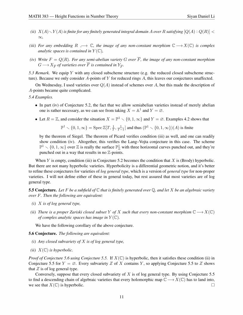
• In part (iv) of Conjecture 5.2, the fact that we allow semiabelian varieties instead of merely abelianone is rather necessary, as we can see from taking X = A1 and Y = ∅.
• Let R = Z, and consider the situation X = P1 r 0, 1,∞ and Y = ∅. Examples 4.2 shows that
P1 r 0, 1,∞ = SpecZ[T, 1T ,
1T−1 ] and thus (P1 r 0, 1,∞)(A) is finite
by the theorem of Siegel. The theorem of Picard verifies condition (iii) as well, and one can readilyshow condition (iv). Altogether, this verifies the Lang–Vojta conjecture in this case. The schemeP1 r 0, 1,∞ over Z is really the surface P1
Z with three horizontal curves punched out, and they’repunched out in a way that results in no Z-points.
When Y is empty, condition (iii) in Conjecture 5.2 becomes the condition that X is (Brody) hyperbolic.But there are not many hyperbolic varieties. Hyperbolicity is a differential geometric notion, and it’s betterto refine these conjectures for varieties of log general type, which is a version of general type for non-propervarieties. I will not define either of these in general today, but rest assured that most varieties are of loggeneral type.
5.5 Conjecture. Let F be a subfield of C that is finitely generated over Q, and letX be an algebraic varietyover F . Then the following are equivalent:
(i) X is of log general type,
(ii) There is a proper Zariski closed subset Y of X such that every non-constant morphism C−→X(C)of complex analytic spaces has image in Y (C).
We have the following corollary of the above conjecture.
5.6 Conjecture. The following are equivalent:
(i) Any closed subvariety of X is of log general type,
(ii) X(C) is hyperbolic.
Proof of Conjecture 5.6 using Conjecture 5.5. If X(C) is hyperbolic, then it satisfies these condition (ii) inConjecture 5.5 for Y = ∅. Every subvariety Z of X contains Y , so applying Conjecture 5.5 to Z showsthat Z is of log general type.
Conversely, suppose that every closed subvariety of X is of log general type. By using Conjecture 5.5to find a descending chain of algebraic varieties that every holomorphic map C−→X(C) has to land into,we see that X(C) is hyperbolic.
11

MATH 383 — Height Functions in Number Theory Siyan Daniel Li
If we assume Conjecture 5.1 and Conjecture 5.6, we can deduce the following conjecture.
5.7 Conjecture (Bombieri–Lang). Let F be a finitely generated field over Q, and let X be a proper varietyof general type over F . Then X(F ) is not Zariski dense in X .
In the curve case, the Bombieri–Lang conjecture is equivalent to the Mordell conjecture, because a pro-jective curve X is of general type if and only if g(X) ≥ 2. I should give some explanation on what generaltype means, shouldn’t I? In the case of non-singular projective hypersurfaces X ⊂ Pn+1 of dimension nand degree m, it is of general type if and only if m ≥ n+ 3.
5.8 Examples. Note that we are working in characteristic zero for the moment.
• For an example with n = 1, note that the Fermat curve
[x : y : z] | xm + ym = zm
is of general type if and only if m ≥ 4.
• For an example with n = 2, we see that
[x : y : z : w] | x5 + y5 + z5 + w5 = 0
is of general type.
Hyperbolic varieties are harder to characterize. There is a conjecture of Kobayashi7 from 1970 thatcharacterizes hyperbolic non-singular projective hypersurfaces as those with sufficiently large m8, given n.
6 January 17, 2018
Last time, I introduced some very general conjectures, and today I’ll discuss some examples and comple-ments of these. I hope to get to the definition of the important notion of log general type from last time.
6.1 Example. Over C, consider the affine variety
X := (x1, . . . , xn+1) |n+1∑i=1
xi = 1, xi 6= 0 for all 1 ≤ i ≤ n+ 1.
Note that when n = 1, this variety becomes P1r0, 1,∞, which we have thoroughly discussed previouslyvia Siegel’s theorem, Examples 4.2, and Examples 5.4. So X is a generalized version of the P1 r 0, 1,∞situation. Recall that our conjectures also involve an auxiliary closed subvariety Y—here, it shall be
Y :=⋃
I⊆1,...,n+12≤#I≤n
YI , where YI = (x1, . . . , xn+1) ∈ X |∑i∈I
xi = 0.
If n = 1, then X is Brody hyperbolic as we have seen before. However,for n ≥ 2 it is not—for example,when n = 2 we have a non-constant holomorphic map
C−→X(C)
t 7−→ (et,−et, 1) ∈ YI for I = 1, 2.
We first proceed to condition (iii) of Conjecture 5.2. Stay in the situation of Example 6.1.7See Conjecture 7.5.8In this sense, perhaps hyperbolic varieties are also quite common—we just don’t understand them as well.
12

MATH 383 — Height Functions in Number Theory Siyan Daniel Li
6.2 Theorem (Borel (1897)). Let f : C−→X is a non-constant morphism of complex analytic spaces, andwrite f = (f1, . . . , fn+1). Then there exists an I as above such that
∑i∈I fi = 0 and the fi for i 6= I are
constant.
This is an improvement on the theorem of Picard, which covered the n = 1 case. Next, what about thealgebraic aspect of Conjecture 5.2? In that situation, take R = Z, and form the finite type Z-scheme
X := SpecR[T1, . . . , Tn,1T1, . . . , 1
Tn, 1T1+···+Tn−1 ].
This recovers the variety X over C from Example 6.1, because we can simply replace xn+1 with 1− x1 −· · · − xn. In general, for any Z-algebra A we have
X(A) = HomZ(Z[T1, . . . , Tn,1T1, . . . , 1
Tn, 1T1+···+Tn−1 ], A)
= a1, . . . , an+1 ∈ A× |n+1∑i=1
ai = 1.
Similarly, form Y =⋃I YI , where the YI are closed subschemes of X cut out by
∑i∈I Ti = 0, respectively
(where Tn+1 = 1− T1 − · · · − Tn). As Conjecture 5.2 predicts, the following result holds (but the proof ishard, and we won’t describe it in class):
6.3 Theorem (Poorten–Schlickewei (1982), Evertse (1984)). The setX(A)rY (A) is finite for any integraldomain A containing Z that is finitely generated over Z.
However, the set X(A) itself might be infinite.
6.4 Example. Let A = Z[12 ] and n = 2. Then X(Z[1
2 ]) contains the infinite subset (2m,−2−m, 1), so thecontent of Theorem 6.3 is that infinite subsets of X(A) only arise from the patterns cut out by the YI , up toan error of finitely many points lying outside of YI(A).
Borel’s theorem and Conjecture 5.5 tell us that XQ should be of log general type.
6.5 Remark. Borel’s theorem shows us thatX(C)rY (C) is Brody hyperbolic. When n = 2, it turns out thatthe related set X(C) r (1,−1, 1), (−1, 1, 1) is Brody hyperbolic but not Kobayashi hyperbolic! So theconverse of Proposition 4.4 is not true in general, even though we remind ourselves that Brody hyperbolicityimplies Kobayashi hyperbolicity when X(C) is compact.
6.6 Remark. Stay in the n = 2 case. Then (X r Z)(A) is always finite, where Z is the union
Z := T1 = 1, T2 = −1 ∪ T1 = −1, T2 = 1.
This can be shown using the theorem of Siegel. Note that that (XrZ)(C) = X(C)r(1,−1, 1), (−1, 1, 1),so Remark 6.5 remains consistent with Conjecture 4.5.
I hope now to explain the notion of log general type. Let F be a field, let X be an algebraic variety overF , and let X be a compactification of X . We begin with the case where X is smooth, and choose X suchthat D := X rX is a divisor with normal crossings. Form the sheaf
Ω1X
(logD) := meromorphic Kahler differentials that are regular on X with at worst log poles at D,
where a meromorphic differential has at worst log poles at D if it is locally of the form
g + h · df
f,
where g is a regular differential, h is a regular function, and f and f−1 are both regular outside of D.
13

MATH 383 — Height Functions in Number Theory Siyan Daniel Li
6.7 Example. Consider the case of X = A1 = SpecF [T ], and write S = 1T . Then D = ∞ is a single
point. If f dT is any differential on X , the quotient rule shows that
f dT = f d( 1S ) = −f dS
S2 .
Therefore here Ω1X
(logD) has no nonzero global sections.
In general, Ω1X
(logD) is a vector bundle of rank n on X , where n is the dimension of X . Thereforeω :=
∧n Ω1X
(logD) is a line bundle on X . We can now define the log Kodaira dimension of X .
6.8 Definition. The log Kodaira dimension of X is defined to be
κ(X) := infk ∈ Z
∣∣∣m 7→ dimF Γ(X,ω⊗m)
mkis a bounded function
.
In general, we have different choices of compactification X . However, the F -vector space Γ(X,ω⊗m) willnot depend on the particular X we choose, so κ(X) is well-defined.
Return now to the case of a general algebraic variety X over F , which might be singular. Assuming theresolution of singularities (which is known for charF = 0), take a proper birational morphism X ′−→X ,where X ′ is smooth, and define κ(X) to be κ(X ′). It turns out that κ(X) is also independent of the X ′
chosen.Finally, use log Kodaira dimension to finally define log general type.
6.9 Definition. We say that X is of log general type if κ(X) = dimX .
6.10 Example. We begin by considering the case of X = P1, using the coordinates from Example 6.7.Suppose F has characteristic not equal to 2, and form the following table of values for Γ(X,ω⊗m):
X Γ(X,ω) Γ(X,ω⊗m) for m ≥ 2
P1 0 0
P1 r ∞ 0 0
P1 r 0,∞ F · dTT F · (dT
T )⊗m
P1 r 0, 1,∞ F · dTT + F · dT
T−1
∑F · (dT
T )⊗a( dTT−1)⊗b
P1 r 0, 1, 2,∞ F · dTT + F · dT
T−1 + F · dTT−2 something with dimension 2m+ 1
Therefore we see that the first three have log Kodaira dimension 0 and thus are not of log general type, whilethe last two have log Kodaira dimension 1 are thus are of log general type.
In general, we have either κ(X) = −∞ or 0 ≤ κ(X) ≤ dimX . Next time, we’ll wrap this up and thenturn to the Vojta conjectures.
7 January 19, 2018
Today, let’s discuss some complements to the notions of log Kodaira dimension and log general type.
7.1 Example. Let F be a field, and form the varietyX as in Example 6.1 over F . As predicted by Conjecture5.5, X is of log general type. To see this, consider the compactification X −→ X := Pn given by
(x1, . . . , xn+1) 7→ [−1 : x1 : · · · : xn].
14

MATH 383 — Height Functions in Number Theory Siyan Daniel Li
Then the divisor D = X rX at infinity isn⋃i=0
xi = 0 ∪ x0 + · · ·+ xn = 0,
so it is indeed a normal crossings divisor. Form ω =∧n Ω1
X(logD) as before, and consider Γ(X,ω⊗m).
Writing
e1 :=dT1
T1, . . . , e1 :=
dTnTn
, en+1 :=d(T1 + · · ·+ Tn − 1)
T1 + · · ·+ Tn − 1=
d(T1 + · · ·+ Tn)
T1 + · · ·+ Tn − 1,
we see that Γ(X,ω) has an F -base given by
αj := ei1 ∧ · · · ∧ ein
for any integers 1 ≤ i1 < · · · < in ≤ n+ 1. In general, Γ(X,ω⊗m) has an F -base given by
αa(1)1 · · ·αa(n+1)
n+1
for any non-negative integers a(i) totaling m. Calculating dimensions via stars and bars gives us
dimF Γ(X,ω⊗m) =
(m+ n
n
)=
(m+ 1) · · · (m+ n)
n!,
which is a polynomial of degree n in m. Therefore κ(X) = n, which shows that X is of log general type.
I haven’t defined what a normal crossing divisor is! In the case of a complex analytic manifold X , thisnotion is relatively easy to explain.
7.2 Definition. Let D be a closed complex analytic submanifold of X . We say D is a normal crossingsdivisor if we can locally identify X with an analytic submanifold of Cn such that, on these charts, D is ofthe form
D = z = (z1, . . . , xn) ∈ Cn |r∏i=1
zi = 0 ∩X =
r⋃i=1
z ∈ Cn | zi = 0
∩Xfor some integer 1 ≤ r ≤ k.
The algebraic theory of normal crossings divisors is more complicated. For this, we begin by discussingthe case of simple normal crossings divisors. Let F be a field, and let X be a smooth variety over F .
7.3 Definition. Let D be a closed subscheme of X . We say that D is a simple normal crossings divisor if,for all x in X , there exists a regular sequence t1, . . . , tk for OX,x such that ID,x is generated by t1, . . . , trfor some integer 1 ≤ r ≤ k, where ID denotes the quasicoherent ideal sheaf corresponding to D.
Observe that Definition 7.3 imitates Definition 7.2. However, to obtain the definition for general normalcrossings divisors in the scheme-theoretic setting, we need to first pass to an etale cover.
7.4 Example. Consider a non-singular hypersurfaceX in Pn+1 of degreem, which is the homogeneous zeroset of a homogeneous polynomial f in F [T1, . . . , Tn+1] of degree m. Then dimX = n, and the Kodairadimension of X turns out to be
κ(X) =
n if m > n+ 2,
0 if m = n+ 2,
−∞ if m < n+ 2,
15
MATH 383 — Height Functions in Number Theory Siyan Daniel Li
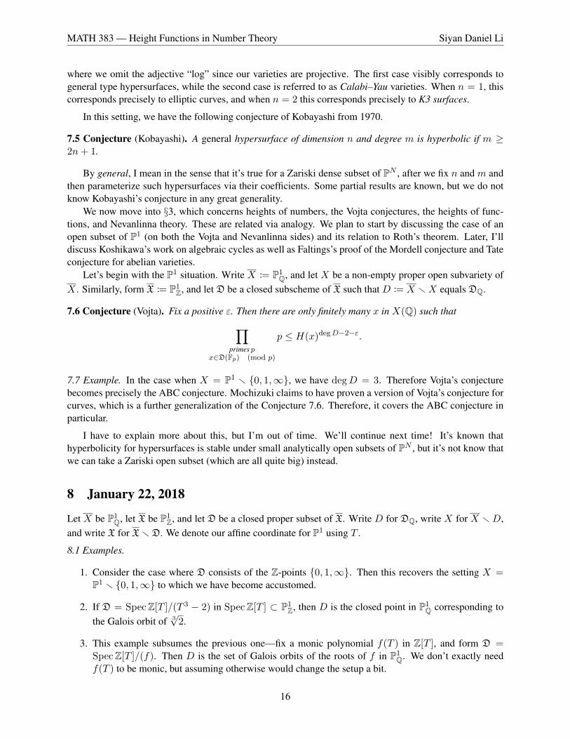
where we omit the adjective “log” since our varieties are projective. The first case visibly corresponds togeneral type hypersurfaces, while the second case is referred to as Calabi–Yau varieties. When n = 1, thiscorresponds precisely to elliptic curves, and when n = 2 this corresponds precisely to K3 surfaces.
In this setting, we have the following conjecture of Kobayashi from 1970.
7.5 Conjecture (Kobayashi). A general hypersurface of dimension n and degree m is hyperbolic if m ≥2n+ 1.
By general, I mean in the sense that it’s true for a Zariski dense subset of PN , after we fix n and m andthen parameterize such hypersurfaces via their coefficients. Some partial results are known, but we do notknow Kobayashi’s conjecture in any great generality.
We now move into §3, which concerns heights of numbers, the Vojta conjectures, the heights of func-tions, and Nevanlinna theory. These are related via analogy. We plan to start by discussing the case of anopen subset of P1 (on both the Vojta and Nevanlinna sides) and its relation to Roth’s theorem. Later, I’lldiscuss Koshikawa’s work on algebraic cycles as well as Faltings’s proof of the Mordell conjecture and Tateconjecture for abelian varieties.
Let’s begin with the P1 situation. Write X := P1Q, and let X be a non-empty proper open subvariety of
X . Similarly, form X := P1Z, and let D be a closed subscheme of X such that D := X rX equals DQ.
7.6 Conjecture (Vojta). Fix a positive ε. Then there are only finitely many x in X(Q) such that∏primes p
x∈D(Fp) (mod p)
p ≤ H(x)degD−2−ε.
7.7 Example. In the case when X = P1 r 0, 1,∞, we have degD = 3. Therefore Vojta’s conjecturebecomes precisely the ABC conjecture. Mochizuki claims to have proven a version of Vojta’s conjecture forcurves, which is a further generalization of the Conjecture 7.6. Therefore, it covers the ABC conjecture inparticular.
I have to explain more about this, but I’m out of time. We’ll continue next time! It’s known thathyperbolicity for hypersurfaces is stable under small analytically open subsets of PN , but it’s not know thatwe can take a Zariski open subset (which are all quite big) instead.
8 January 22, 2018
Let X be P1Q, let X be P1
Z, and let D be a closed proper subset of X. Write D for DQ, write X for X rD,and write X for XrD. We denote our affine coordinate for P1 using T .
8.1 Examples.
1. Consider the case where D consists of the Z-points 0, 1,∞. Then this recovers the setting X =P1 r 0, 1,∞ to which we have become accustomed.
2. If D = SpecZ[T ]/(T 3 − 2) in SpecZ[T ] ⊂ P1Z, then D is the closed point in P1
Q corresponding tothe Galois orbit of 3
√2.
3. This example subsumes the previous one—fix a monic polynomial f(T ) in Z[T ], and form D =SpecZ[T ]/(f). Then D is the set of Galois orbits of the roots of f in P1
Q. We don’t exactly needf(T ) to be monic, but assuming otherwise would change the setup a bit.
16

MATH 383 — Height Functions in Number Theory Siyan Daniel Li
By viewing D as scheme over Z9, we can form D(Fp), which is defined by the same equation. Recall thatwe have a reduction map P1(Q)−→P1(Fp). Vojta’s conjecture for Example 8.1.2 implies that the sets
(a, b) ∈ Z2 | a3 − 2b3 = 1 and (a, b) ∈ Z2 | a3 − 2b3 = −3
are finite. To see this, the conjecture itself says that∏primes p
x∈D(Fp) (mod p)
p ≤ H(x)1−ε
for only finitely many x in X(Q), since degD = 3. Writing x = a/b for coprime integers a and b, we seethat
x (mod p) ∈ D(Fp) ⇐⇒ (a/b)3 ≡ 2 (mod p) ⇐⇒ a3 − 2b3 ≡ 0 (mod p).
Now the (a, b) lying in our sets of interest only have the prime 3 (at most) dividing a3 − 2b3. Therefore thequantity ∏
primes px∈D(Fp) (mod p)
p
is bounded from above by 3. Recalling from Lecture 2 there are only finitely many x with bounded height,we see that Vojta’s conjecture concludes the proof.
Note that this also shows that X(Z[ 1N ]) is finite for degD > 2, since
X(Z[ 1N ]) = x ∈ X(Q) | x (mod p) /∈ D(Fp) for p - N.
Thus the Vojta conjecture encapsulates our earlier conjecture conjectures and results.Let us discuss the connection with geometry. In our P1 setting, recall from Proposition 3.2 that X(C)
is hyperbolic if and only if degD ≥ 3. In turn, one can extend Example 6.10 to show that this occursif and only if X is of log general type. The degD ≥ 3 condition here coincides with the condition thatdegD − 2 = deg(Ω1
X(logD)) > 0, which is an important criterion in the general Vojta conjectures.
The following theorem of Roth also follows from Vojta’s conjecture:
8.2 Theorem (Roth). Let α be an algebraic number, which we view as a complex number, and fix a positivenumber ε. Then there are only finitely many rational numbers x satisfying
|x− α| ≤ 1
H(x)2+ε.
This is a statement that limits how well we can approximate algebraic numbers using rational numbers.
8.3 Example. While this example can be proven rather elementarily, we could use Roth’s theorem to showthat
α =
∞∑n=0
1
10n!
is transcendental, because the series∑∞
n=m1
10n!approximates α too well for α to be algebraic.
9With any scheme structure we like—see Remark 5.3.
17
MATH 383 — Height Functions in Number Theory Siyan Daniel Li
Proof sketch of Roth’s theorem using Vojta’s conjecture. One can reduce to the case where α is an algebraicinteger, so assume this is the case. Let f(T ) be the monic irreducible polynomial of α over Q. Furthermore,assume that α lies in R, since otherwise of course we cannot approximate α by rational numbers.Integralityimplies that f(T ) has coefficients in Z. Applying Vojta’s conjecture to the situation of Example 8.1.3 tellsus that cofinitely many rational numbers x satisfy∏
x∈D(Fp) (mod p)
p ≥ H(x)degD−2−ε,
where D and D are as in Example 8.1. Now write
f(T ) = Tn + c1Tn−1 + · · ·+ cn
for some integers ci. Writing x = a/b for coprime integers a and b, emulating the above calculation forf(T ) in place of T 3 − 2 shows that
Nx := |an + an−1c1b+ · · ·+ cnbn| ≥
∏x (mod p)∈D(Fp)
p.
Next, form Mx := max|f(x)|−1, 1. Then Mx is large if and only if f(x) is close to zero, which occurs ifand only if x is close to some conjugate of α. It turns out that we roughly have
MxNx ∼ H(x)degD,
where ∼ means that both sides bound one another up to a constant factor. We should view Mx as anarchimedean contribution and Nx as a nonarchimedean contribution. Combining our estimate for Nx withour estimate from Vojta’s conjecture yields
Nx & H(x)degD−2−ε =⇒ Mx . H(x)2+ε =⇒ |x− α| ∼M−1x &
1
H(x)2+ε.
I will flesh out this argument next time.
The weaker estimate Nx & H(x)dimD−2−ε that we used above is actually known unconditionally to betrue, so this yields Roth’s theorem unconditionally. The main difference between this weaker estimate andthe Vojta conjecture itself is that Nx might not just contain the primes p involved in∏
x (mod p)∈D(Fp)
p
with multiplicity 1 but rather with some very high multiplicity. We can already see this phenomenon in theabove situation, as Nx is the sum of many high powers.
9 January 24, 2018
Last time, I started explaining how Roth’s theorem is a special case of Vojta’s conjecture. I was usingsome bad notation, so let me now use some better notation. Keeping everything else from Lecture 8 unlessotherwise specified, write
HD,∞(x) := max|f(x)|−1, 1HD,f (x) := |an + c1a
n−1b+ · · ·+ cnbn|
HD(x) := HD,∞(x)HD,f (x),
where our notation is now much more suggestive of the archimedean and nonarchimedean contributions.We have the following three key points:
18
MATH 383 — Height Functions in Number Theory Siyan Daniel Li
(1) Note that ∏p is primep|HD,f (x)
p =∏
p is primex∈D(Fp) (mod p)
p divides HD,f (x),
divides HD,f (x). However, the above product of primes does not contain the multiplicity of the primesdividing HD,f (x), i.e. it is the radical of HD,f (x).
(2) We roughly have HD(x) ∼ H(x)degD, where we note that degD = deg f . More precisely:
9.1 Proposition. There exists positive numbers C1 and C2 such that
C1H(x)degD ≤ HD(x) ≤ C2H(x)degD
for all x in Q such that f(x) 6= 0.
I will not prove this, but the key step is
HD(x) = max
∣∣∣∣∣(a
b
)n+ · · ·+ cn
∣∣∣∣∣−1
, 1
|an + · · ·+ cnbn|
= max
|b|n
|an + · · ·+ cnbn|, 1
|an + · · ·+ cnb
n| = max|b|n, |an + · · ·+ cnbn|.
One immediately sees that we can set C2 := max|c1|, . . . , |cn|, 1, since H(x) = max|a|, |b|. Theother direction also becomes relatively straightforward.
(3) When |x− α| is small enough, we have |x− α| ∼ HD,∞(x)−1. This is the case because
f(x) =
deg f∏i=1
(x− αi),
where the αi range over the conjugates of α over Q. When |x− α| is small, the value |f(x)|−1 blows upfrom the |x− α|−1 contribution (while the other factors stay bounded), so this term is what HD,∞(x)equals. The constants involved in ∼ comes from considering these other factors∏
αi 6=α|α− αi|.
9.2 Remark. If f(T ) equals the polynomial T , then HD(x) equals the height H(x) of x as defined before.To see this, take
HD(x) = max|x|−1, 1|a| = max| ba |, 1 = max|b|, |a| = H(x).
Now that we have elucidated these three key points, the proof of Roth’s theorem of Vojta’s conjecture followsas in Lecture 8.
We can also interpret HD,f (x) as
HD,f (x) =∏
p is prime
HD,p(x),
19
MATH 383 — Height Functions in Number Theory Siyan Daniel Li
where HD,p(x) := max|f(x)|−1p , 1 for the normalized p-adic norm |·|p. Therefore HD(x) can be written
as
HD(x) =∏
v a place of QHD,v(x) =⇒ H(x) =
∏v a place of Q
max|x|−1v , 1 =
∏v a place of Q
max1, |x|v, (?)
where the last equality is due to the product formula. This segues nicely into our next topic: heights on Pn!
9.3 Definition. Let x lie in Pn(Q), and write x as [a0 : · · · : an] for some integers ai such that (a0, . . . , an) =1. Then the height of x, which we denote using H(x), is defined to be
H(x) := max|a0|, · · · , |an|.
9.4 Proposition. For all real B, the set
x ∈ Pn(Q) | H(x) ≤ B
is finite.
I don’t have time to discuss heights in further detail today, so we’ll conclude by giving examples ofinteresting questions about heights you could study instead. Let X be a closed subvariety of Pn over Q, andlet X be a dense open subset of X . The following conjecture was studied by Manin and Tschinkel, whereManin studied the a part and Tschinkel studied the b part.10
9.5 Conjecture (Manin–Tschinkel). There exist real numbers a, b, and c such that
#x ∈ X(Q) | H(x) ≤ B = cBa log(B)b(1 + o(1))
as B →∞.
For another interesting question, we also have a more general conjecture of Vojta. Let X be a closedsubset of P1
Z, and let X be a dense open subset of X. Write D := X r X, and form their respective basechanges X , X , and D to Q. There is a version of Conjecture 7.6 that continues to use heights, but this timethe exponent of H(x) is related to
∧m Ω1X
(logD) (as we remarked in Lecture 8), where m is the dimensionof X . I’ll explain this in detail next time.
10 January 26, 2018
Today, I’ll continue talking about heights in Pn over a number field. In the situation of a general numberfield F , it’s not generally possible to take a representative of x in Pn(F ) of the form [a0 : · · · : an] with(a0, . . . , an) = 1, by the failure of unique factorization. In this situation, we adopt the perspective ofEquation (?), and define heights using the following product over all places.
10.1 Definition. Let x = [a0 : · · · : an] be a point of Pn(F ). We say the height of x (relative to F ) is
HF (x) :=∏
v a place of F
max|a0|v, . . . , |an|v,
where we normalize the absolute values to be the “big” ones, i.e. the ones that make the complex places thesquare of the usual absolute value on C. By the product formula, HF (x) is well-defined.
10For further discussion, see Lecture 13.
20
MATH 383 — Height Functions in Number Theory Siyan Daniel Li
In the case of F = Q, Equation (?) shows that we recover our previous definition of H(x).
10.2 Proposition. For any finite extension F ′ of F and x in F , we have HF ′(x) = HF (x)[F ′:F ].
Proof. For all places v′ of F ′ lying over a place v of F , we have |x|v′ = |x|[F′v′ :Fv ]
v . Therefore this equalityfollows from the sum formula
∑v′|v[F
′v′ : Fv] = F .
10.3 Definition. Let x be a point of Pn(Q). We say the (absolute) height of x is H(x) := HF (x)1/[F :Q],where F is any number field over which x is defined.
Proposition 10.2 shows that the map H : Pn(Q)−→R>0 is well-defined. Now this H map is verycomplicated—for instance, it’s certainly far from being continuous for the complex topology on P1(Q), butthat makes sense because that’s just the topology induced from one place. Similar statements would beexpected and indeed true at the nonarchimedean places, for instance.
10.4 Example. Consider the n = 1 situation. Here, we define the height of any x in Q via taking the heightof [x : 1] in P1(Q). The algebraic numbers α satisfying [Q(α) : Q] ≤ 2 of smallest height are
α H(α)
0,±1,±2,±ζ23 1
±1±√
52
√1+√
52
Note that the second row includes the golden ratio, and its low height encapsulates its simplicity. Thissimplicity appears to our eyes, even if we don’t explicitly compute its height. Small numbers give us somebeauty.
Our eyes can enjoy 2-dimensional beauty, but our ears are not so good for this. Our ears detect sound,which comes from time and hence is 1-dimensional.
do re mi fa so1 12
√2
12√
22 12√
23 12√
24
These ratios are good when used by pianos, but for the harmony of human voices, it may be better to use
do:mi do:fa do:so5:4 4:3 3:2
On the other hand, the piano needs even-tempering for the changing of keys. The problem of which system isbetter is probably why ancient Greek mathematicians discovered irrational numbers. To them, mathematicsand music were the same subject.
The following theorem is an important generalization of Proposition 9.4.
10.5 Theorem. Fix n, fix d, and fix a positive number C. Then
x ∈ Pn(Q) | H(x) ≤ C and x is defined over a field of degree at most d
is a finite set. In particular, x ∈ Pn(F ) | HF (x) ≤ C is finite for any number field F .
I will not prove it, but the idea is to bound the possible coefficients for the minimal polynomial of any xin the above set using our constraints.
10.6 Example. The sequence H(21/n) is bounded, which does not contradict Theorem 10.5 because thedegrees of 21/n are unbounded.
21
MATH 383 — Height Functions in Number Theory Siyan Daniel Li
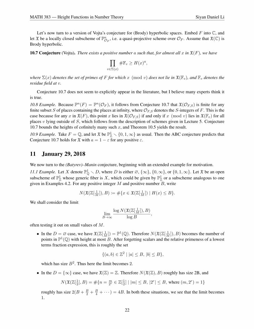
Let’s now turn to a version of Vojta’s conjecture for (Brody) hyperbolic spaces. Embed F into C, andlet X be a locally closed subscheme of PnOF , i.e. a quasi-projective scheme over OF . Assume that X(C) isBrody hyperbolic.
10.7 Conjecture (Vojta). There exists a positive number a such that, for almost all x in X(F ), we have∏v∈Σ(x)
#Fv ≥ H(x)a,
where Σ(x) denotes the set of primes of F for which x (mod v) does not lie in X(Fv), and Fv denotes theresidue field at v.
Conjecture 10.7 does not seem to explicitly appear in the literature, but I believe many experts think itis true.
10.8 Example. Because Pn(F ) = Pn(OF ), it follows from Conjecture 10.7 that X(OF,S) is finite for anyfinite subset S of places containing the places at infinity, whereOF,S denotes the S-integers of F . This is thecase because for any x in X(F ), this point x lies in X(OF,S) if and only if x (mod v) lies in X(Fv) for allplaces v lying outside of S, which follows from the description of schemes given in Lecture 5. Conjecture10.7 bounds the heights of cofinitely many such x, and Theorem 10.5 yields the result.
10.9 Example. Take F = Q, and let X be P1Z r 0, 1,∞ as usual. Then the ABC conjecture predicts that
Conjecture 10.7 holds for X with a = 1− ε for any positive ε.
11 January 29, 2018
We now turn to the (Batyrev)–Manin conjecture, beginning with an extended example for motivation.
11.1 Example. Let X denote P1Q rD, where D is either ∅, ∞, 0,∞, or 0, 1,∞. Let X be an open
subscheme of P1Z whose generic fiber is X , which could be given by P1
Z or a subscheme analogous to onegiven in Examples 4.2. For any positive integer M and positive number B, write
N(X(Z[ 1M ]), B) := #x ∈ X(Z[ 1
M ]) | H(x) ≤ B.
We shall consider the limit
limB→∞
logN(X(Z[ 1M ]), B)
logB,
often testing it out on small values of M .
• In the D = ∅ case, we have X(Z[ 1M ]) = P1(Q). Therefore N(X(Z[ 1
M ]), B) becomes the number ofpoints in P1(Q) with height at most B. After forgetting scalars and the relative primeness of a lowestterms fraction expression, this is roughly the set
(a, b) ∈ Z2 | |a| ≤ B, |b| ≤ B,
which has size B2. Thus here the limit becomes 2.
• In the D = ∞ case, we have X(Z) = Z. Therefore N(X(Z), B) roughly has size 2B, and
N(X(Z[12 ], B) = #n = m
2r ∈ Z[12 ] | |m| ≤ B, |2r| ≤ B, where (m, 2r) = 1
roughly has size 2(B + B2 + B
4 + · · · ) = 4B. In both these situations, we see that the limit becomes1.
22

MATH 383 — Height Functions in Number Theory Siyan Daniel Li
• In the D = 0,∞ case, we have have
N(X(Z[12 ]), B) = #±2m | 2|m| ≤ B ∼ 4
logB
log 2.
Therefore the limit here is 0.
• In the D = 0, 1,∞ case, the set X(Z[ 1M ]) is finite by Siegel’s theorem. Therefore the limit here is
0.
This behavior is related to the sheaf Ω1P1Q(logD) on P1
Q. Recall that we have an isomorphism OP1Q(−2(∞))
∼−→Ω1P1Q
given by f 7→ f dT . We can see this from the descriptions
Ω1P1Q(U) = f dT | f has no poles on U and OP1
Q(−2(∞)) = f | f + 2(∞) ≥ 0 restricted to U,
where U is any open subset of P1Q, because the coordinate S = 1
T at infinity satisfies dS = −dT/T 2.Therefore we have Ω1
P1Q(logD) ∼= OP1
Q(D − 2(∞)). Furthermore, note in our examples that
limB→∞
logN(X(Z[ 1M ]), B)
logB= max2− degD, 0.
We are now ready to present the Manin conjecture in general. Let F be a number field, let X be anirreducible smooth closed subscheme of PnF , let D be a normal crossings divisor of X , and write X :=X rD. Furthermore, let X be a locally closed subscheme of PnOF whose generic fiber is X . Set
α := s ∈ Q≥0 | cl(ω) + s · cl(H) is effective,
where ω denotes∧dimX Ω1
X(logD), and H is the hyperplane associated to our choice of height function
H .11 I will explain these notions next time—for now, let us just proceed to the conjecture.
11.2 Conjecture (Batyrev–Manin). There exists a finite extension F1 of F and a finite set of places S1 ofF1 containing the archimedean places such that, for any finite extension F ′ of F1 and finite set S′ of placesof F ′ containing those lying above S1, then there exists a proper closed subscheme Y of X such that
limB→∞
#x ∈ X(OF ′,S′) | x /∈ Y (F ′), H(x) ≤ BlogB
= α.
In the case when X has dimension 1, the subscheme Y has dimension 0, so the x /∈ Y (F ′) conditiondoes not change this limit, as it only affects finitely many points. However, this may not be true in general.
12 January 31, 2018
We shall continue discussing the Batyrev–Manin conjecture today, and for this we begin with some prelim-inaries on divisors and line bundles. Let k be a field, and let V be a connected proper smooth algebraicvariety over k.
12.1 Definition. A divisor is a formal finite sum∑
P aP · P , where the aP are integers and P ranges overclosed irreducible codimension 1 subvarieties of V . We write Div(V ) for the abelian group of divisors onV , which is a free abelian group on the set of P .
11This definition of α is incorrect as given here—see Lecture 12.
23

MATH 383 — Height Functions in Number Theory Siyan Daniel Li
For any f in k(V )×, we write
Div(f) :=∑P
ordP (f)P,
where ordP (f) is the order of f at P . We define ordP (f) via the normalized valuation induced from thediscrete valuation ring OV,v, where v is the generic point of P . We define the divisor class group C`(V ) viathe exact sequence
k(V )×Div−→Div(V )−→C`(V )−→ 0.
On the other hand, for any D =∑
P aPP in Div(V ), write OV (D) for the sheaf of OV -modules given by
U 7→ f ∈ k(V ) | ordP (f) + aP ≥ 0 for all v ∈ U.
Then OV (D) is a line bundle, i.e. it is locally isomorphic to OV as an OV -module. Form the set
Pic(V ) := isomorphism classes of line bundles on V,
which becomes an abelian group under tensor products. We get an isomorphism C`(V )∼−→Pic(V ) given
by sending D 7→ OV (D).
12.2 Example. Let V = P1k with the coordinate T , and consider the sheaf Ω1
V on V . It is a line bundle on Vbecause it is OV dT when restricted to Spec k[T ] and OV d( 1
T ) when restricted to Spec k[ 1T ]. However, it is
not the trivial line bundle. In fact, we can show that Ω1V∼= OV (−2(∞)).
For simplicity in defining the Neron–Severi group, assume that k lies in C. Then we can form thecomplex manifold V (C), and we define the Neron–Severi group to be
NS(V ) := im(C`(V )−→H2(V (C),Z)),
where the map is given by sending P to the cohomology class of P (C). In particular, this map factorsthrough C`(V ). This may be an analytic construction, but it can be made algebraic in some way that I won’tspecify.
12.3 Example. When dimV = 1, the Neron–Severi group embeds into H2(V (C),Z) = Z, and it’s theimage of the map sending P to deg(P ) := [k(P ) : k]. Therefore if k is algebraically closed, we see thatNS(V ) equals the entirety of H2(V (C),Z).
In the setting of general V , the sheaf of Kahler differentials Ω1V is a vector bundle of rank n, where
n := dimV . Therefore the canonical class ω :=∧n Ω1
V is a line bundle on V .
12.4 Definition. We say a divisor K on V is canonical if its corresponding line bundle is isomorphic to ω.For any normal crossings divisor D of V , we say that K +D is log canonical for (V,D) or for V rD.
It can be shown that the line bundle corresponding to K +D is isomorphic to∧n Ω1
V (logD).
12.5 Example. Suppose that V = Pnk , and let H ⊂ Pnk be the hyperplane corresponding to [a0 : · · · : an]in Pn(k). Then the isomorphism class of the line bundle corresponding to H is independent of H , and wedenote it using OPnk (1). The isomorphism class corresponding to K equals −(n+ 1) times OPnk (1).
Next, suppose that V is now a closed subscheme of Pnk . If H is a hyperplane that does not contain V ,then we say V ∩ H is a hyperplane section of V . In this situation, the line bundle associated to V ∩ H isindependent of H , and it equals the pullback of OPnk (1) to V .
24

MATH 383 — Height Functions in Number Theory Siyan Daniel Li
Next, let F be a number field, which we view as a subfield of C. Let X be a connected smooth closedsubvariety of PNF . Let D be a normal crossings divisor on X , and write X := X r D. Write n for thedimension of X . Here comes my first mistake—the definition of α should have been
α := infs ∈ R≥0 | cl(K +D) + s · cl(H) ∈ NS(X)R-eff,
where NS(X)R-eff is the closure in NS(X)⊗Z R of the subset
NS(X)R-eff := m∑i=1
ai cl(Ei) | ai ≥ 0, Ei is an effective divisor on X.
We remark that NS(X)R-eff might be generated by rays of of slope tending towards a limit, so NS(X)R-effitself might not be closed. I’m not sure how Vojta came up with α in the formulation of his conjectures, butin any case it’s a very geometric (rather than arithmetic) quantity.
Finally, let X be a locally closed subscheme of PNOF whose generic fiber is X , and let X be the closureof X in PNOF . Now that we have the right setup, we can state the Batyrev–Manin conjecture, which actuallycomes with two parts:
12.6 Conjecture (Batyrev–Manin).
(1) Assume that α is positive. Then if F ′ ⊇ F is a sufficiently large number field, then if S is a sufficientlylarge finite set of places of F ′ containing the archimedean ones, then if Y is a sufficiently large properclosed subset of X , then
limB→∞
#x ∈ X(OF ′,S) | x /∈ Y (F ′), H(x) ≤ BlogB
= α.
In the Batyrev–Manin, I’m not sure whether the S or Y should come first, that is, which “sufficientlylarge” condition depends on which. I’ll get to the next part of the conjecture next time.
13 February 2, 2018
Last time, I was stating the conjecture of Batyrev and Manin. Recall that α is some real number that wasdefined in a highly geometric manner. I stated the conjecture for positive α, but I didn’t get to finish.
13.1 Conjecture (Batyrev–Manin). Keeping our setup from before,
(2) If α is zero, then for any finite set of places S of F containing the archimedean places and any positiveε, there exists a proper closed subset Y of X such that
#x ∈ X(OF,S) | x /∈ Y (F ), H(x) ≤ BBε
is a bounded function of B.
More on the Batyrev–Manin conjecture can be found in their article “Sur le nombre des points rationnelsde hauteur borne.” In the case when X = X is proper, we see that X(OF,S) = X(F ), so we can replaceX(OF,S) with X(F ) in the Batyrev–Manin conjecture.
25

MATH 383 — Height Functions in Number Theory Siyan Daniel Li
13.2 Example. Consider the case X = X = PnF . In this case, α = n + 1, because in this case Pic(Pn) isisomorphic to Z, where any integer a corresponds to the isomorphism class of the line bundle correspondingto any hyperplane H . Thus we see that NS(PnF )R-eff equals R≥0. Furthermore, the canonical divisor K ofPnF has class equal to −(n+ 1) times the class of H , and here D = ∅. Altogether we see that α = n+ 1.
The case of a general number field F is difficult to understand, so let us specialize to F = Q. Then
#x = [a0 : · · · : an] ∈ Pn(Q) | H(x) = max|a0|, . . . , |an| ≤ B ∼ Bn+1,
where we choose a0, . . . , an satisfying (a0, . . . , an) = 1. Therefore we see that the Batyrev–Manin conjec-ture indeed holds for PnQ.
13.3 Example. Let X = X be a projective (which is the same thing as proper in this case, and I’ll movebetween these readily) smooth curve over F , and embed X as a subvariety of PmF . Example 12.3 shows thatNS(X)R-eff consists of the preimage of R≥0 ⊂ H2(X(C),R) = R in NS(X)R. Therefore
NS(X)R-eff = R≥0,
and because here the degree of K is 2g − 2 (where g is the genus of X), we see that
α =
0 if g ≥ 1,⌊2
degH
⌋if g = 0,
where H is a hyperplane section (that is, a closed point) of X with minimal degree.Now suppose that g = 1, and write E for X . Then the theory of elliptic curves tells you that
#x ∈ E(F ) | H(x) ≤ B = c log(B)r/2(1 + o(1)),
where r is the Mordell–Weil rank of E(F ). Taking the limit from the Batyrev–Manin conjecture indeedyields 0, because the extra log factor kills the rank term regardless.
For g ≥ 2, the Mordell conjecture tells us that #X(F ) is finite, which verifies the conjecture too, andwe have dealt with the g = 0 case in Example 13.2 (assuming Example 13.2 extends to general F ), sincehere X = P1
F if and only if it has rational points at all.
13.4 Example. If X is of log general type, then the class of K + D always already lies in NS(X)R-eff, sohere α = 0. Recall that the definition of X being of log general type is equivalent to
∧n Ω1X
(logD) beingbig, whose definition we give below.
13.5 Definition. Let L be a line bundle on X . We say that L is big if
κ(L ) := inf
s ∈ Z | m 7→ dim Γ(X,L ⊗m)
msis a bounded function
equals dimX .
The notion of height zeta functions are important in this subject, so we review it now.
13.6 Definition. Let Λ be a set, and let H : Λ−→R>0 be a map. Their height zeta function is defined to be
ZΛ,H(s) :=∑x∈Λ
1
H(x)s,
ignoring convergence issues for now.
26

MATH 383 — Height Functions in Number Theory Siyan Daniel Li
13.7 Example. In our setup, we take Λ to be X(OF,S) and H to be the usual absolute height function:
• When X = P1Z, then the resulting height zeta function is
ZP1(Q),H(s) =4ζ(s− 1)
ζ(s),
where ζ is the Riemann zeta function. To see this, note that
ZP1(Q),H(s) =∞∑n=1
#x ∈ P1(Q) | H(x) = nns
=∞∑n=1
4ϕ(n)
ns= 4
ζ(s− 1)
ζ(s),
where ϕ denotes the Euler phi function.
In general, suppose that we can write ZΓ,H as
ZΓ,H(s) =c
(s− a)b+
g(s)
(s− a)b−1
for some non-negative real number a, positive integer b, positive real number c, and holomorphic functiong(s) on the domain s ∈ C | Re(s) > a − S for some positive S. The ZΓ,H(s) absolutely converges forRe(s) > a, and we have
#x ∈ Γ | H(x) ≤ B =c
a(b− 1)!Ba log(B)b−1(1 + o(1)),
where our asymptotic is taken with respect to B.
13.8 Example. Consider the situation of Example 13.7. As
ζ(s) =1
s− 1+ a holomorphic function
around s = 1, we see that
ZP1(Q),H(s) = 4ζ(s− 1)
ζ(s)=
4
ζ(2)
1
s− 2+ a holomorphic function
around s = 2. Then a = 2, b = 1, and c = 4/ζ(2), so we have
#x ∈ P1(Q) | H(x) ≤ B =4
2ζ(2)B2(1 + o(1)) =
12
π2B2(1 + o(1)).
The method of zeta functions is very powerful. Batyrev–Manin further conjectured that a = α. Theyalso have some conjectures concerning b, but they are very complicated, so I do not plan to discuss them inclass.
14 February 5, 2018
Let us now discuss the height functions associated to line bundles. Next time, we’ll investigate a questionthat Olivier brought up after class last time, since it’s an interesting question that I spent a lot of time thinkingabout. I would do it now, but he’s not here, so that’d be weird.
Let F be a number field, and let X be a smooth closed subvariety of PnF . Let D be a normal crossingsdivisor of X , and form X := X rD. As usual, let X be a locally closed subscheme of PnOF whose genericfiber is X . We have the following general conjecture of Vojta.
27

MATH 383 — Height Functions in Number Theory Siyan Daniel Li
14.1 Conjecture (Vojta). Let ε be positive. Then there exists a proper closed subset Y of X such that, forcofinitely many x in X(F ) r Y (F ), we have ∏
v a primex∈X(Fv) (mod v)
#Fv
1/[F :Q]
≥ HK+D(x)H(x)−ε,
where H denotes our absolute height as before, and HK+D has not yet been explained yet.
For any proper algebraic variety V over F and line bundle L on V , we shall obtain a height function
HL : V (F )−→R>0,
via constructing a height function HF,L : V (F )−→R>0 and setting HL := H1/[F :Q]F,L . The exponent’s role
is to ensure that we can repeat this for all finite extensions F ′/F and get a well-defined function HL .
14.2 Example. If V = X and L =∧dimX Ω1
X(logD), thenHL yields the desiredHK+D in the statement
of Vojta’s conjecture.
14.3 Example. If V = PnF and L is the line bundle associated to a hyperplane H , then the resulting HL isthe usual absolute height on PnF .
Well, these examples are not exact on the nose—the height function HL depends on certain choicesmade. However, for any such choices, the resulting height functions HL and H ′L shall satisfy HL ∼ H ′L ,that is, there exists C ≥ 1 such that
C−1HL (x) ≤ H ′L (x) ≤ CHL (x)
for all x in V (F ). What exactly are these choices? Well, let us fix
• a metric |·|v on L for each archimedean place v,
• an integral structure of L (which can be replaced by a norm |·|v on L for each non-archimedeanplace v, indicating that this is an analog of the first choice).
14.4 Example. Let us first consider the case when V = SpecF is a point. Then line bundles L on V arejust 1-dimensional vector spaces. Let L is a 1-dimensional F -vector space. Then an integral structure on Lis just the choice of a finitely-generated OF -submodule LOF of L, and a metric |·|v for archimedean v is amap L⊗v C−→R≥0 such that
• |ax|v = |a|v|x|v for all a in F and x in L, where now we use the “small” absolute value for |a|v,
• |x|v 6= 0 for x 6= 0.
Then the associated height function (which is just a single value, because V (F ) = V (F ) is just a point) is
HF (L) := #(LOF /OFx)∏v|∞
|x|−1v
for any nonzero x in LOF , which is independent of the choice of x.
14.5 Example. Let F = Q in Example 14.4, let |·|∞ be the usual absolute value, let L = Q, and let LZ ben−1Z for any n ≥ 1 in Z. Taking x = 1 shows that HQ(L) = n.
28

MATH 383 — Height Functions in Number Theory Siyan Daniel Li
For another presentation of Example 14.4, let v be a non-archimedean place of F . Choose a basis e of theOF,(v)-module LOF,(v) := OF,(v) ⊗OF LOF , and let |x|v := |x/e|v, where the right-hand side denotes theusual “small” absolute value. We see that
HF (L) =∏
v a place of F
|x|−1v ,
which is independent of the choice of x because any two choices differ by an element of F×, and the productformula implies that this doesn’t change HF (L).
Now let’s tackle case of general varieties, where we begin by discussing metrics at the archimedeanplace. Let V now be a proper algebraic variety over C, and let L be a line bundle on V .
14.6 Definition. A metric on L is a morphism of sheaves
|·|L : L top−→CR≥0,
where L top is the sheaf of topological sections of the (geometrically realized) line bundle L on V (C), andCR≥0 is the sheaf of R≥0-valued continuous functions on V (C), such that
• |fλ|L = |f ||λ|L for any sections f of CR≥0 and λ of L ,
• if λ is a nonvanishing section of L , then |λ|L is a nonvanishing section of CR≥0.
I only have five minutes left, so I can’t treat the nonarchimedean condition yet.
14.7 Example. For V = P1C and L = OV ((∞)), the assignment
|f |L (x) :=|f(x)|
max1, |x|
yields a metric on L . This shall be the metric that we use to obtain the usual absolute height on P1F .
I didn’t get time to do so today, but next time I’ll discuss the nonarchimedean component of this heightfunction construction.
15 February 7, 2018
Last time, we were trying to set up general height functions on proper varieties V over a number field F , butit’s easier when V is actually projective, so we make this assumption from now on. Let L be a line bundleon V . Recall that we were trying to construct an associated height function
HL : V (F )−→R>0,
and that while this construction depends on some choices, these choices yield equivalent functions under therelation ∼. The choices we need to make are:
• a metric |·|L in the sense of Definition 14.6 on L over V (F v) for all archimedean place v of F ,
• a projective scheme VOF overOF whose generic fiber is isomorphic to V and a coherentOF -moduleon VOF whose generic fiber, under the previous identification, is isomorphic to L .
Recall that, for a locally Noetherian scheme, a coherent module is one that correspond to finitely generatedmodules on affine patches.
29

MATH 383 — Height Functions in Number Theory Siyan Daniel Li
15.1 Example. Such objects do exist. For instance, we can take the Zariski closure of V in PnOF for VOF ,where we view V as living inside PnF .
15.2 Definition. Using the above choices, we construct
HF,L : V (F )−→R>0
as follows. For any x in V (F ), form the fiber L (x) of L at x, which is a 1-dimensional F -vector space.Then set
HF,L (x) := HF (L (x)),
where HF denotes the function from Example 14.4 constructed using the pullbacks of the norms ‖·‖L andthe integral structures VOF and LOF to SpecF via x.
15.3 Example. Let V be PnF , and let L be OPnF (1). Let’s choose VOF to be PnOF , and let LOF be OPnOF(1),
which is formed in the same way as OPnF (1), except that you use OF throughout instead of F . WriteT0, . . . , Tn for the homogeneous coordinates of Pn, and let Uj be the affine patch where Tj is nonzero. Wewrite
x = [x1 : · · · : xj−1 : 1 : xj+1 : · · · : xn]
for any F -point of Uj , where the x1, . . . , xj , . . . , xn lie in F . Note that x is anOF -point if and only if thesex1, . . . , xj , . . . , xn actually lie in OF . In this situation, we have
LOF (x) = OFx1 + · · ·+OFxj−1 +OFxj+1 + · · ·+OFxn,
so for any nonarchimedean place v of F we get LOF,v(x) = OF,ve, where e is any element of F satisfying
|e|v = max|x1|v, . . . , |xj−1|v, 1, |xj+1|v, . . . , |xn|v.
Of course, for general F -points x, we have L (x) = F .Let’s now turn to the archimedean contribution. For any section f of L , let |·|L on V (F v) be the metric
given by sending
|f |F (x) :=|f(x)|
max|x1| . . . , |xj−1|, 1, |xj+1|, . . . , |xn|.
With this metric in hand, we see that HF,L (x) = HF (L (x)) is well-defined.
15.4 Definition. We extend our height functions to V (F ) by defining
HL (x) := HF ′,L ′(x)1/[F ′:F ],
where F ′ is any number field for which x lies in V (F ′), L ′ is the base change of L to VF ′ , and we constructHF ′,L ′ using the pullbacks of our choices for V and L over F .
Now that we have completed a description of the theory of height functions, Conjecture 14.1 makessense. Mochizuki’s statements on Conjecture 14.1 actually involve a stronger, uniform claim for x′ inV (F ′) for number fields F ′ with bounded [F ′ : F ]. I’ll discuss this next time. Also, I never heard back onnews of Mochizuki’s paper.
30

MATH 383 — Height Functions in Number Theory Siyan Daniel Li
16 February 12, 2018
Given all the conjectures we’ve introduced in the course, it’s always nice to see what these conjecturesconcretely mean.
16.1 Example. Let n ≥ 4 be an integer, and consider the situation where
X = P2Z r xn0 + xn1 + xn2 = 0 = SpecZ[T1, T2]/(Tn1 + Tn2 + 1)
Then X := XQ is of log general type, and we see that
X(Z[ 1N ]) = [x0 : x1 : x2] ∈ P2(Q) | gcdx0, x1, x2 = 1, xn0 + xn1 + xn2 ∈ Z[ 1
N ]×.
Conjecture 5.2 and Conjecture 5.5 together predict that there exists a proper closed subscheme Y of X suchthat
x ∈ X(Z[ 1N ]) | x /∈ Y (Q)
is finite. Furthermore, these conjectures predict that this Y can be taken to be the smallest closed subset ofX such that any non-constant holomorphic map f : C−→X(C) has image in Y (C). I expect this Y equals
Y = xn0 + xn1 = 0 ∪ xn0 + xn2 = 0 ∪ xn1 + xn2 = 0,
as we have a holomorphic map C−→X(C) given by t 7→ [t : αt : 1], where α is an n-th root of −1. In thecase when n = 5 and N = 2, we also see that X(Z[ 1
N ]) is infinite, because it contains the elements
[2m : −2m : 1]
for all integers m. This infinitude would also be blocked by punching out Y . If my description of Y iscorrect, then X(Z[ 1
N ]) should be finite when n = 4, for arbitrary N . More strongly, I expect that
(x, y, z) ∈ Z3 | gcdx, y, z = 1, xn + yn + zn ∈ Z[13 ]× = ±(0, 0, 1), ±(1, 0, 0), ±(0, 1, 0), ±(1, 1, 1)
for any n ≥ 4. My evidence for believing this is that it holds for max|x|, |y|, |z| ≤ 4 and n = 4.
Let’s use the Vojta conjectures as not evidence (as they’re not proven), but rather support for this con-jecture. Suppose that n ≥ 16 and that 4|n. As background motivation, consider the following result ofLegendre, which was originally stated by Fermat.
16.2 Theorem (Legendre). If m is an integer that cannot be written as 4a(8b+ 7) or any integers a and b,then m can be written as a sum of three perfect squares.
Returning to Example 16.1, rewrite our desired condition as
(xn/4)4 + (yn/4)4 + (zn/4)4 ∈ Z[13 ]×.
At this point, let X be the n = 4 case of the original setup (not our new n ≥ 16 setup), and let Y be theproper closed subset of X given to us by Conjecture 14.1.
16.3 Remark. In the case when X is of log general type, it is conjectured that the Y appearing in Conjecture5.2 and Conjecture 5.5 can be taken to be the same as the one appearing in Conjecture 14.1. I am not sure ifthis conjecture is written down in Vojta’s papers, however.
31

MATH 383 — Height Functions in Number Theory Siyan Daniel Li
Anyways, choosing a small ε and using Conjecture 14.1 shows that cofinitely many of our desired triples(x, y, z) satisfy
∏p|(xn+yn+zn)
p ≥ C max|x|n/4, |y|n/4, |z|n/4
1−ε
for some constant C. Our N = 3 condition implies that the left-hand side is at most 3, which wouldnarrowly bound the possibilities for (x, y, z). In general, this problem seems very hard—we can think ofit as a second Fermat’s last theorem. It’s can’t be the first Fermat’s last theorem, because that’s alreadybeen solved, but this seems just as hard. Furthermore, you can readily obtain many second Fermat’s lasttheorems, by changing N from 3 to 2 or 5.
Returning to general principles, let’s discuss the height functions appearing in Conjecture 14.1 and theline bundles appearing in their formulation. Recall the situation of Definition 13.5. Let V be a projectivevariety over a field F , and let L be a line bundle on V .
16.4 Definition. We say that L is
• very ample if it is the pullback of the canonical bundle on PM for some closed embedding V −→ PM ,
• ample if L ⊗k is very ample for some positive integer k.
For any divisor D on V , we say that D is very ample, ample, or big if the line bundle OV (D) has thecorresponding property.
We relate bigness to ampleness.
16.5 Proposition. Ample line bundles are also big. Furthermore, a divisor B is big if and only for anyample divisor A, there exists positive integers b and a and an effective divisor E such that
b · OV (B) = a · OV (A) + OV (E)
in Pic(V ), and this is also equivalent to saying that there exists some positive integer b, ample divisor A,and effective divisor E satisfying
b · OV (B) = OV (A) + OV (E).
16.6 Example. Let X be a smooth quasiprojective variety, let X −→ Pn be a compactification of X suchthat D := X rX is a normal crossings divisor of X , and let K be a canonical divisor of X . Recall fromExample 13.4 thatX being of log general type is equivalent to saying thatK+D is big, so Proposition 16.5indicates that we can find positive integers b and a such that
b(K +D) ∼ aA+ E,
where A is the ample divisor of a hyperplane section of X , and E is some effective divisor.
We can combine Example 16.6 with the following statement on heights to decompose HK+D in termsof the standard height on Pn.
16.7 Proposition. Suppose everything is over a number field F . For any divisorsD1 andD2 onX , we haveHD1+D2 ∼ HD1HD2 .
32

MATH 383 — Height Functions in Number Theory Siyan Daniel Li
In the situation of Example 16.6, we see that HA corresponds to the standard height on Pn. Thereforewe can replace the
HK+D(x)H(x)−ε
on the right-hand side of Conjecture 14.1 with
H(x)a/b−εHE(x)1/b.
Outside of E, there exists a constant C such that HE ≥ C, because its archimedean contribution is alwaysbounded above by some constant on V (F ), and its non-archimedean contribution is bounded above by someconstant on (V r E)(F ).
Next time, I’ll probably introduce Nevanlinna theory, and on Friday I’ll probably discuss the Mordellconjecture and its proof.
17 February 14, 2018
I’ll introduce Nevanlinna theory today. I hope you can appreciate the mysterious connection between num-ber theory and analysis that it helps to formulate. Recall from Lecture 2 that
a theorem of Siegel←→ a theorem of Picard,
where Siegel says that x ∈ Q | x, 1 − x ∈ Z[ 1N ]× is finite, and Picard says that any holomorphic map
C−→P1(C) r 0, 1,∞ is constant. A finer version of the above analogy is given by
Vojta’s conjecture (namely, Conjecture 14.1)←→ a conjecture of Griffiths.
17.1 Example. In the case of X = P1 r0, 1,∞, for which Conjecture 14.1 becomes the ABC conjecture,Griffith’s conjecture asks the following question. For any non-constant holomorphic map f : C−→P1(C),how often does f(α) lie in 0, 1,∞?In the case of general varieties, let X be a projective smooth variety over a number field F as usual, let D bea normal crossings divisor of X , and form X := X rD as before. We’ll also fix models X and D for theseobjects over OF . Then the question of Griffiths becomes: given a holomorphic function f : C−→X(C)that is nonconstant, how often do we have f(α) in D(C)? Recall that on the number theory side, Conjecture14.1 relates the quantity ∏
v is primex∈D(Fv) (mod v)
#Fv
with the height of x associated to certain line bundles. We can construct a similar notion of height functionsin the analytic setting. To remove uninteresting cases, suppose that the image of C under f does not lie inD(C).
17.2 Definition. The analog of the above product of primes on the Nevanlinna side is the quantity
N(1)f,D(r) :=
∑α∈C|α|<r
f(α)∈D(C)
log r|α| if α 6= 0,
log r if α = 0,
where r is any non-negative number. Since D is a normal crossings divisor and f(C) does not lie in D(C),we see that f−1(D(C)) has codimension 1 in C, that is, it is discrete. Thus its intersection with |z| < r isfinite, so N (1)
f,D(r) is indeed a finite sum.
33

MATH 383 — Height Functions in Number Theory Siyan Daniel Li
17.3 Example. In the setting of P1r0, 1,∞, we could consider functions f : C−→P1(C) like f(z) = ez
or f(z) = zn for integers n ≥ 1.
As for the analog of the arithmetic height function, let L be a holomorphic line bundle on X(C). Justlike the arithmetic situation, our height function (which we denote using f 7→ Tf,L (r)) depends on a choiceof metric on L , but different metrics yield functions that are equivalent under∼, where the implied constantis independent of f and r. Griffiths’s conjecture then becomes that we roughly always have
N(1)f,D(r) ≥ Tf,K+D(r).
17.4 Example. Recall the situation of Example 17.3. In this situation, line bundles are classified by degree,and degK = −2 and degD = 3. Therefore K +D is a hyperplane class.
(1) For f(z) = ez , note that f never hits 0 nor∞. Then we only need to consider 1, and for this we see that
N(1)f,D(r) =
(2
⌊r
2π
⌋+ 1
)log r − 2 log
(⌊r
2π
⌋!
)− 2
⌊r
2π
⌋log 2π.
We will see in Example 18.2 that
Tf,K+D(r) = Tf,H(r) =r
π,
so the Griffiths conjecture indeed holds in this case. However, it barely holds—Stirling’s formula im-plies that
N(1)f,D(r)− Tf,K+D(r)→ 0
as r →∞.
(2) For f(z) = zn when n is a positive integer, note that f(z) = 0 only at z = 0 and that f(z) = 1 preciselyfor the n-th roots of unity. Therefore for r > 1, we have
N(1)f,D(r) = (n+ 1) log r,
and it turns out in Example 18.2
Tf,H(r) = n log r
in this case, which once again verifies Griffiths’s conjecture.
We shall now turn to actually defining Tf,L (r). Let V be a projective smooth complex manifold, let Lbe a holomorphic line bundle on V equipped with a metric |·|L , and let f : C−→V be a holomorphic map.Write L = OV (D) for some divisor D on V such that f(C) is not contained in the support of D.
17.5 Definition. Let r be positive. The function Tf,L (r) is defined to be
Tf,L (r) := mf,D(r) +Nf,D(r),
wheremf,D(r) is the analog of the archimedean component of arithmetic heights, andNf,D(r) is the analogof the non-archimedean component. We shall define these two components below.
34

MATH 383 — Height Functions in Number Theory Siyan Daniel Li
GAGA tells us that our complex analytic setup is actually algebraic, and we can choose a generator 1for L on the Zariski open subset U := V r suppD of V . Write W = log |1|−1
L , which is a real-valuedfunction on U . Then we get a function
W f : Cr some discrete set(= f−1(D))−→R
because the image of f is not contained in the support of D. We define
mf,D(r) :=1
2π
ˆ 2π
0dθ (W f)(reθi),
which converges because the singularities of W f when considered as a function on all of C are “mild” ina manner we shall not describe. Finally, we define
Nf,D(r) :=∑α∈C|α|<r
ordα(f∗D)
log r|α| if α 6= 0,
log r if α = 0.
Note that Nf,D(r) is almost exactly equal to N (1)f,D(r), except now we count the multiplicity with which f
reaches a value α rather than just always weight it as 1.
18 February 16, 2018
Let’s recall the setup of Nevanlinna theory. Let V be a smooth projective algebraic variety over C, and letf : C−→V (C) be an analytic morphism. Let L be a line bundle on V (C), which we take to be algebraic,although GAGA tells us this is the same as taking a holomorphic vector bundle on V (C). Then we havedefined a height function Tf,F (r) for all positive r, and while this function depends on the choice of agenerator of L (U) for U = V r suppD as well as a metric |·|L on L , different choices give equivalentfunctions under the relation ∼.
Today, we’ll cover some examples of these functions. WriteD for a divisor of V such that L = OV (D),and choose D such that f(C) is not contained in the support of D. As the absolute value of the generator|1|L on U goes to ∞ as we approach suppD, we see that W = log |1|−1
L goes to −∞. Therefore themf,D(r) term measures how close f gets to suppD, where this value is more negative when f gets closerto suppD. This is analogous to the inversion of the archimedean sizes in, say, Example 14.4, and this isalso why we say that mf,D(r) is an analog of the archimedean contribution.
The philosophy on Nf,L is that it measures how often the function f crosses suppD on C, whereasmf,L measures how f crosses suppD at infinity. Our motivation is further solidified by Jensen’s formula:
18.1 Proposition (Jensen). For any meromorphic function g : C 99K C, we have
∑|α|<r
ordα(g)
log r|α| if α 6= 0,
log r if α = 0,=
1
2π
ˆ 2π
0dθ log |g(reiθ)| − “ log |g(0)|”,
where “log |g(0)|” is the leading coefficient of the Laurent expansion of g.
Thus we can also interpret mf,D(r) as trying to count hits of f on D on the neighborhood of∞ whoseboundary is the circle of radius r around the origin. We write U(0) for “log |g(0)|”. You can also useJensen’s formula to show that Tf,L (r) is independent of the choice of D.
35
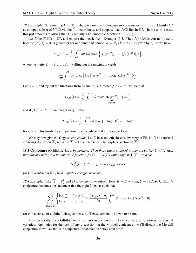
MATH 383 — Height Functions in Number Theory Siyan Daniel Li
18.2 Example. Suppose that V = PnC, where we use the homogeneous coordinates z0, . . . , zn. Identify Cnas an open subset of V (C) via the 0-th coordinate, and suppose that f(C) lies in Cn. (In the n = 1 case,this just amounts to asking that f is actually a holomorphic function C−→C.)
Let D be Pn(C) r Cn, and choose the metric from Example 15.3. Then Nf,D(r) is constantly zero,because f∗(D) = 0. A generator for our bundle of choice L = OV (D) on Cn is given by z0, so we have
Tf,L (r) =1
2π
ˆ 2π
0dθ log max
|f1(reiθ)|, . . . , |fn(reiθ)|, 1
,
where we write f = (f1, . . . , fn). Pulling out the maximum yields
1
2π
ˆ 2π
0dθ max
log |f1(reiθ)|, . . . , log |fn(reiθ)|, 0
.
Let n = 1, and try out the functions from Example 17.3. When f(z) = ez , we see that
Tf,L (r) =1
2π
ˆ 2π
0dθ maxRe(reiθ)︸ ︷︷ ︸
r cos θ
, 0 =r
π,
and if f(z) = zm for an integer m ≥ 1, then
Tf,L (r) =1
2π
ˆ 2π
0dθ maxm log r, 0 = m log r
for r ≥ 1. This finishes a computation that we advertised in Example 17.4.
We may now give the Griffiths conjecture. LetX be a smooth closed subvariety of PnC, letD be a normalcrossings divisor on X , set X := X rD, and let H be a hyperplane section of X .
18.3 Conjecture (Griffiths). Let ε be positive. Then there exists a closed proper subvariety Y of X suchthat, for any real c and holomorphic function f : C−→X(C) with image in Y (C), we have
N(1)f,D(r) ≥ Tf,K+D(r)− εTf,H(r) + c
for r in a subset of R≥0 with cofinite Lebesgue measure.
18.4 Example. Take X = P1C and D to be any finite subset. Here K + D ∼ (degD − 2)H , so Griffiths’s
conjecture becomes the statement that the right Y exists such that
∑|α|<rf(α)∈D
log r|α| if α 6= 0,
log r if α = 0,≥ (degD − 2)
2π
ˆ 2π
0dθ maxlog |f(reiθ)|, 0
for r in a subset of cofinite Lebesgue measure. This statement is known to be true.
More generally, the Griffiths conjecture known for curves. However, very little known for generalvarieties. Apologies for the lack of any discussion on the Mordell conjecture—we’ll discuss the Mordellconjecture as well as the Tate conjecture for abelian varieties next time!
36
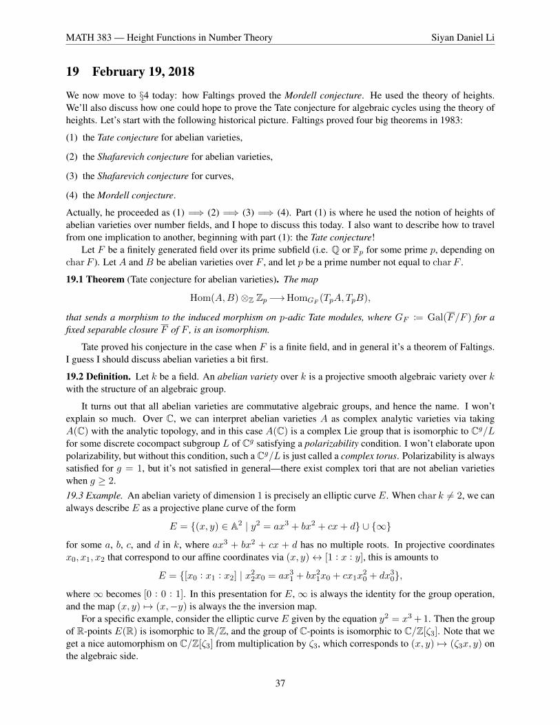
MATH 383 — Height Functions in Number Theory Siyan Daniel Li
19 February 19, 2018
We now move to §4 today: how Faltings proved the Mordell conjecture. He used the theory of heights.We’ll also discuss how one could hope to prove the Tate conjecture for algebraic cycles using the theory ofheights. Let’s start with the following historical picture. Faltings proved four big theorems in 1983:
(1) the Tate conjecture for abelian varieties,
(2) the Shafarevich conjecture for abelian varieties,
(3) the Shafarevich conjecture for curves,
(4) the Mordell conjecture.
Actually, he proceeded as (1) =⇒ (2) =⇒ (3) =⇒ (4). Part (1) is where he used the notion of heights ofabelian varieties over number fields, and I hope to discuss this today. I also want to describe how to travelfrom one implication to another, beginning with part (1): the Tate conjecture!
Let F be a finitely generated field over its prime subfield (i.e. Q or Fp for some prime p, depending oncharF ). Let A and B be abelian varieties over F , and let p be a prime number not equal to charF .
19.1 Theorem (Tate conjecture for abelian varieties). The map
Hom(A,B)⊗Z Zp−→HomGF (TpA, TpB),
that sends a morphism to the induced morphism on p-adic Tate modules, where GF := Gal(F/F ) for afixed separable closure F of F , is an isomorphism.
Tate proved his conjecture in the case when F is a finite field, and in general it’s a theorem of Faltings.I guess I should discuss abelian varieties a bit first.
19.2 Definition. Let k be a field. An abelian variety over k is a projective smooth algebraic variety over kwith the structure of an algebraic group.
It turns out that all abelian varieties are commutative algebraic groups, and hence the name. I won’texplain so much. Over C, we can interpret abelian varieties A as complex analytic varieties via takingA(C) with the analytic topology, and in this case A(C) is a complex Lie group that is isomorphic to Cg/Lfor some discrete cocompact subgroup L of Cg satisfying a polarizability condition. I won’t elaborate uponpolarizability, but without this condition, such a Cg/L is just called a complex torus. Polarizability is alwayssatisfied for g = 1, but it’s not satisfied in general—there exist complex tori that are not abelian varietieswhen g ≥ 2.19.3 Example. An abelian variety of dimension 1 is precisely an elliptic curve E. When char k 6= 2, we canalways describe E as a projective plane curve of the form
E = (x, y) ∈ A2 | y2 = ax3 + bx2 + cx+ d ∪ ∞
for some a, b, c, and d in k, where ax3 + bx2 + cx + d has no multiple roots. In projective coordinatesx0, x1, x2 that correspond to our affine coordinates via (x, y)↔ [1 : x : y], this is amounts to
E = [x0 : x1 : x2] | x22x0 = ax3
1 + bx21x0 + cx1x
20 + dx3
0,
where∞ becomes [0 : 0 : 1]. In this presentation for E,∞ is always the identity for the group operation,and the map (x, y) 7→ (x,−y) is always the the inversion map.
For a specific example, consider the elliptic curve E given by the equation y2 = x3 + 1. Then the groupof R-points E(R) is isomorphic to R/Z, and the group of C-points is isomorphic to C/Z[ζ3]. Note that weget a nice automorphism on C/Z[ζ3] from multiplication by ζ3, which corresponds to (x, y) 7→ (ζ3x, y) onthe algebraic side.
37

MATH 383 — Height Functions in Number Theory Siyan Daniel Li
Let A be an abelian variety over F of dimension g. For any n such that charF does not divide n, it is afact that its n-torsion subgroup satisfies
A(F )[n] := ker(n : A(F )−→A(F )) ∼= (Z/nZ)2g.
In the case when F −→ C, we can see this from the lattice description via
A(C)[n] = ker(n : Cg/L−→Cg/L) = ( 1nL)/L ∼= (Z/nZ)2g.
In the setting of general fields F , we naturally have a Galois action on A(F ).
19.4 Example. Return to our concrete elliptic curve from Example 19.3. When n = 2, its 2-torsion is
E(Q)[2] = ∞, (−ζa3 , 0)
as a ranges through 0, 1, 2. Thus we get a nontrivial Galois action already, and this Galois action onlygets bigger (i.e. the subgroup acting trivially gets smaller) as we increase n.
19.5 Definition. The p-adic Tate module of A, denoted using TpA, is defined to be
TpA = lim←−n
A(F )[pn],
where the transition maps are given by multiplication by p.
If p is a prime such that charF does not divide p, our previously stated fact indicates that TpA isisomorphic to Z2g
p as a Zp-module. In the situation where F −→ C, our description of A(C)[n] yields
TpA = lim←−n
A(C)[pn] = lim←−n
( 1pnL)/L = lim←−n L/p
nL = L⊗Z Zp.
Furthermore, note that H1(Cg/L,Z) = L, so we can rewrite the Tate module as H1(Cg/L,Z) ⊗Z Zp =H1(Cg/L,Zp). This reformulation leads to the Tate conjecture for general algebraic varieties:
19.6 Conjecture (Tate conjecture for algebraic cycles). Let F be a field that is finitely generated over itsprime subfield, and let X be a proper smooth algebraic variety over F . Then for all primes p such thatcharF does not divide p, the cycle map
CHr(X)⊗Z Qp−→(H2r
et (XF ,Qp)(r))GF
,
where CHr(X) denotes the r-th Chow group of codimension r algebraic cycles modulo rational equiva-lence, and (r) denotes a Tate twist, is surjective.
For the remainder of my life, I hope to study this conjecture via studying the “heights of the motiveH2r(X)(r).” Maybe you can pick it up too—you’re young. Koshikawa has shown that this general conjec-ture of Tate follows from some finitude statements for heights on motives.
Now how does this conjecture of Tate relate to the Tate conjecture for abelian varieties from earlier?Injectivity is already known for the Tate module map, so the whole statement lies in surjectivity. By takingX = A×B and sending h in Hom(A,B) to its graph, we obtain an element of CHg(X)⊗ZQp. Interpretingp-adic Tate modules asH1
et((−)F ,Qp)∨ and using the Kunneth formula to decomposeH2g
et (XF ,Qp) allowsus to obtain the Tate conjecture for abelian varieties as stated earlier.
Let’s now turn to the Shafarevich conjecture for abelian varieties. Let F be a number field, and let S bea finite set of places of F containing the archimedean ones. Let g be a positive integer.
38
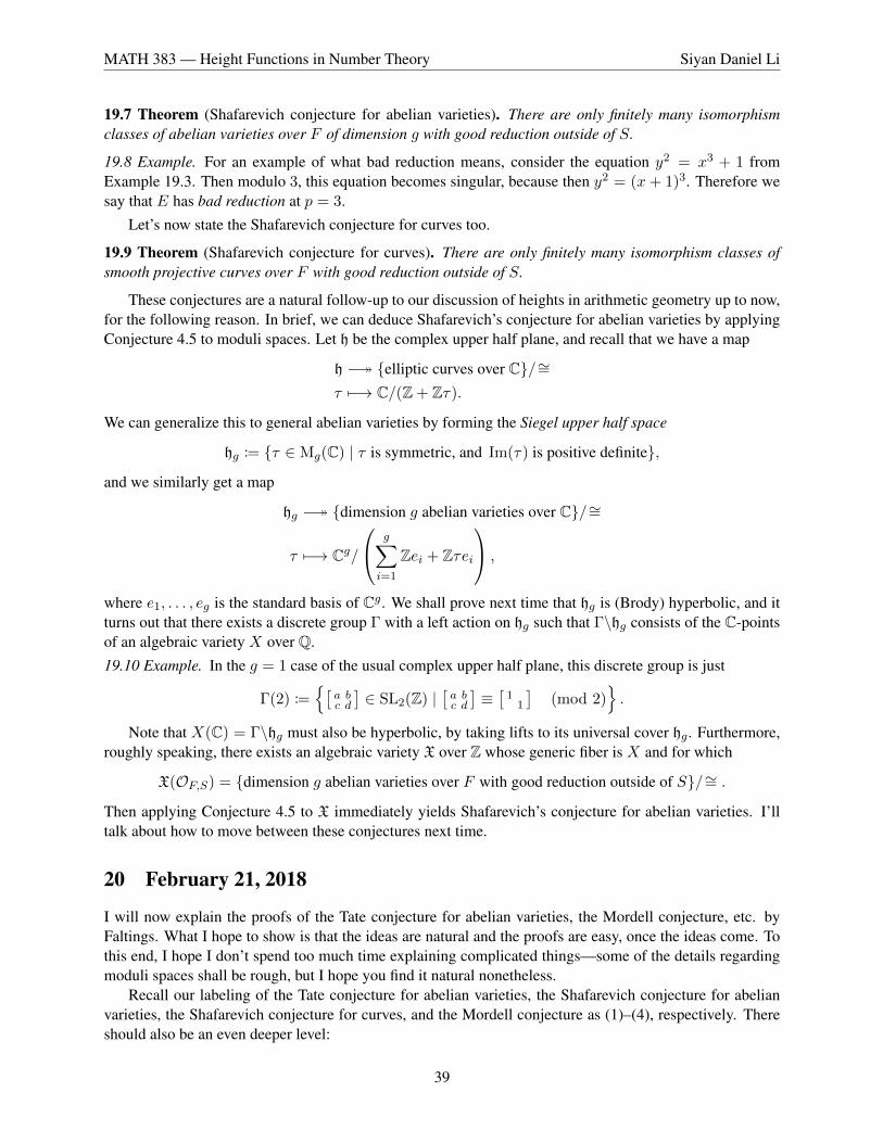
MATH 383 — Height Functions in Number Theory Siyan Daniel Li
19.7 Theorem (Shafarevich conjecture for abelian varieties). There are only finitely many isomorphismclasses of abelian varieties over F of dimension g with good reduction outside of S.
19.8 Example. For an example of what bad reduction means, consider the equation y2 = x3 + 1 fromExample 19.3. Then modulo 3, this equation becomes singular, because then y2 = (x+ 1)3. Therefore wesay that E has bad reduction at p = 3.
Let’s now state the Shafarevich conjecture for curves too.
19.9 Theorem (Shafarevich conjecture for curves). There are only finitely many isomorphism classes ofsmooth projective curves over F with good reduction outside of S.
These conjectures are a natural follow-up to our discussion of heights in arithmetic geometry up to now,for the following reason. In brief, we can deduce Shafarevich’s conjecture for abelian varieties by applyingConjecture 4.5 to moduli spaces. Let h be the complex upper half plane, and recall that we have a map
h − elliptic curves over C/∼=τ 7−→ C/(Z + Zτ).
We can generalize this to general abelian varieties by forming the Siegel upper half space
hg := τ ∈ Mg(C) | τ is symmetric, and Im(τ) is positive definite,
and we similarly get a map
hg − dimension g abelian varieties over C/∼=
τ 7−→ Cg/
g∑i=1
Zei + Zτei
,
where e1, . . . , eg is the standard basis of Cg. We shall prove next time that hg is (Brody) hyperbolic, and itturns out that there exists a discrete group Γ with a left action on hg such that Γ\hg consists of the C-pointsof an algebraic variety X over Q.19.10 Example. In the g = 1 case of the usual complex upper half plane, this discrete group is just
Γ(2) :=[
a bc d
]∈ SL2(Z) |
[a bc d
]≡[
11
](mod 2)
.
Note that X(C) = Γ\hg must also be hyperbolic, by taking lifts to its universal cover hg. Furthermore,roughly speaking, there exists an algebraic variety X over Z whose generic fiber is X and for which
X(OF,S) = dimension g abelian varieties over F with good reduction outside of S/∼= .
Then applying Conjecture 4.5 to X immediately yields Shafarevich’s conjecture for abelian varieties. I’lltalk about how to move between these conjectures next time.
20 February 21, 2018
I will now explain the proofs of the Tate conjecture for abelian varieties, the Mordell conjecture, etc. byFaltings. What I hope to show is that the ideas are natural and the proofs are easy, once the ideas come. Tothis end, I hope I don’t spend too much time explaining complicated things—some of the details regardingmoduli spaces shall be rough, but I hope you find it natural nonetheless.
Recall our labeling of the Tate conjecture for abelian varieties, the Shafarevich conjecture for abelianvarieties, the Shafarevich conjecture for curves, and the Mordell conjecture as (1)–(4), respectively. Thereshould also be an even deeper level:
39

MATH 383 — Height Functions in Number Theory Siyan Daniel Li
(0) finitude of isomorphism classes of abelian varieties in any given isogeny class,
as well as the following variant of the Tate conjecture:
(1)’ for any two abelian varieties A and A′, if VpA is isomorphic to VpA′, then A and A′ are isogeneous.
I will explain these additional ingredients. It’s not easy to discern all these points (as well as the implicationsbetween them) from papers written on their proofs, and I hope to make this all clearer. The proofs go like(0) =⇒ (1) =⇒ (1)’ and (0)+(1)’ =⇒ (2). Let’s now backtrack and define the terms involved.
20.1 Definition. Let A and A′ be abelian varieties over a field k. We say that A and A′ are isogeneous andwrite A ∼ A′ if there exist homomorphisms f : A−→A′ and g : A′−→A and a positive natural number nsuch that g f = f g = n.
20.2 Example. Let k = C, let A be C/Z[ζ3], and let A′ = C/(Z + nZ[ζ3]). There is a canonical quotientmap g : A′−→A, and the map C−→C given by multiplication by n induces a map f : A−→A′. We seethen that f and g witness the fact that A and A′ are isogeneous.
We can now make sense of (0):
20.3 Theorem. Let F be a field that is finitely generated over Q or F`, and let A be an abelian variety overF . Then the set A′ abelian variety over F | A′ ∼ A/∼= is finite.
Part (0) is actually the hardest part of Faltings’s proofs, and he proved it using the theory of heights. Itwas known beforehand the case when F is finite by Tate, and the implication (0) =⇒ (1) was also knownby Tate.12 The second implication (1) =⇒ (1)’ is also relatively accessible. While it’s not easy to extractthis from the literature, I want to give the feeling that everything is easy. It’s a nice feeling.
Sketch of (1) =⇒ (1)’. We can turn an isomorphism VpA ∼= VpA′ into an injective morphism TpA −→ TpB
with finite cokernel, after multiplying by some power of p. The Tate conjecture then yields the mapA−→Bup to Zp-coefficients, and multiplying out the previous factor of p (along with passing down to Z-coefficientssomehow) gives the desired result.
We shall focus on the cases when F is actually finite over its prime subfield, that is, F is either a numberfield or a finite field. In the latter case, part (0) is evident because the entire set
abelian varieties of dimension g over F/∼= = X(F )
is finite, where X is the moduli space of abelian varieties of dimension g. This is true because X is some-thing like an algebraic variety, roughly speaking. When F more generally is finitely generated over a finitefield, a similar argument works by considering F geometrically. On the other hand, when F is a numberfield, it contains no “base” field, so we cannot play such tricks.
Therefore let us move to the situation when F is a number field F , and let’s begin our rough discussionof the moduli space of abelian varieties of dimension g. Our hg has another description:
hg∼−→z ∈ Mg(C) | z is symmetric, 1− tz · z is positive definite
τ 7→ z := (τ − i)(τ + i)−1.
The inverse of the above map sends z 7→ τ := i(1 + z)(z − z)−1.
20.4 Example. When g = 1, this alternative description of h is z ∈ C | |z| < 1, which is precisely thebounded open disk model of the Poincare upper half plane.
12We shall discuss (0) =⇒ (1) in Lecture 22.
40

MATH 383 — Height Functions in Number Theory Siyan Daniel Li
Our bounded realization of hg shows that it is (Brody) hyperbolic, since Liouville’s theorem indicatesthat bounded holomorphic functions are constant.
20.5 Example. In the g = 1 case, the map realizing complex tori as elliptic curves over C yields an isomor-phism
Γ(2)\h ∼−→elliptic curves over C/∼= = P1(C) r 0, 1,∞,
where the last identification is given by the parameter λ in the Legendre form y2 = x(x − 1)(x − λ) of anelliptic curve over C. Now P1 r 0, 1,∞ is a nice convenient scheme X over Z, and for any ring R, weroughly have
elliptic curves over R/∼= = X(R) = Hom(Z[λ, 1λ(1−λ) ], R) = λ ∈ R× | 1− λ ∈ R×.
I will not explain what an elliptic curve over a general ring is. However, for any number field F and finiteset of places S of F containing the archimedean ones, we do have
elliptic curves over OF,S/∼= = elliptic curves over F with good reduction outside S/∼=
via taking Neron models. Our above description (along with Siegel’s theorem) tells you that this set is finite.
Returning to the situation of arbitrary g, we can play a similar game, which we indeed played last time.This showed us that, if we knew Conjecture 4.5, then we would have (2) as a consequence. So (2) is natural.
It’s a fact that isogeneous abelian varieties have good reduction at the same places, which follows fromthe converse of (1)’ (which is immediate) and the Neron–Ogg–Shafarevich criterion:
20.6 Proposition (Neron–Ogg–Shafarevich criterion). Let A be an abelian variety over F , and let v - p bea prime. Then the Galois representation VpA is unramified at v if and only if A has good reduction at v.
In the general setting of abelian varieties, the Neron–Ogg–Shafarevich criterion is a theorem of Serre–Tate. Thus if the abelian variety A over F of dimension g is given, and if S is the finite set of bad reductionplaces of A (together with the infinite places), we see that
A′ abelian variety over F | A′ ∼ A/∼=−→A′ abelian variety over F | dimA = g, A′ has good reduction outside of S.
The latter set is finite by (2), so we see one could actually deduce (0) from (2) as well.What actually happened was that we eventually deduced (2) from (0). And Faltings proved (0) itself
roughly as follows: he took the moduli space X of abelian varieties of dimension g (well, there’s all sortsof additional data like polarizations, endomorphisms, and level structure involved, but we’ll pretend thatall doesn’t exist), which is a projective variety X −→ Pn, and he studied heights on X . He found that ifA′ ∼ A, then most of the time H(A′) = H(A), where H(−) denotes the naive height of the F -point on Xcorresponding to A, and he proved that
H(A′) | A′ ∼ A
is finite. Coupled with Theorem 10.5, we’d obtain (0).. . . Well, the above sketch is not quite true. What Faltings actually did was define the Faltings height
HFal(A), which is an improved version of H(A) that’s roughly the equal to H(A). He then he used HFal tocarry out the above strategy. We’ve run out of time now, but I’ll continue discussing this next time.
41

MATH 383 — Height Functions in Number Theory Siyan Daniel Li
21 February 23, 2018
Let us restrict to the case where F is a number field for today. I hope to finish this course by the end of nextweek! Recall that we cursorily described (1) =⇒ (1)’ last time.
Sketch of (0)+(1)’ =⇒ (2). By (0), it suffices to prove that
A abelian variety over F | dimA = g, A has good reduction outside of S/∼
is finite. Now (1)’ indicates that A modulo ∼ is determined by VpA, and we may assume that the primesabove p lie in S, because this only enlarges the above set of interest. By the Neron–Ogg–Shafarevichcriterion, our condition becomes equivalent to asking that VpA is unramified outside of S. Thus it wouldsuffice to show that only finitely many isomorphism classes (that is, conjugacy classes) of continuous Galoisrepresentations GF −→GL2g(Qp) are unramified outside of S.
By taking Tate twists, we see that this preliminary statement is utterly false. However, we know theweight of VpA, as it is a Galois representation of weight −1. That is, for any v not in S, the characteristicpolynomial of geometric Frobenius has coefficients in Z, and its roots have size #F1/2
v for all complexabsolute values on Qp. Once we restrict the weight of our Galois representations, the number of suchobjects is finite. The proof of this uses the Chebotarev density theorem as well as reduction modulo pfrom GL2g(Zp) to GL2g(Z/pZ). I shall not explain more here, but this is a standard technique in numbertheory.
The proof of (2) =⇒ (3) follows immediately from the fact that
smooth projective curves of genus g with good reduction outside of S/∼=−→abelian varieties of dimension g with good reduction outside of S/∼=,
where the map sends C to its Jacobian JC . And what is the Jacobian, you ask? The general constructionover arbitrary fields is complicated, but for the situation over C, we can proceed with complex geometry asfollows:
21.1 Definition. LetC be a smooth projective curve over C of genus g. Its Jacobian, as a complex manifold,is defined by
JC(C) :=HomC(Γ(C,Ω1
C),C)
H1(C(C),Z)≈ HomC(Cg,C)
Z2g= Cg/Z2g,
where the embedding H1(C(C),Z)−→HomC(Γ(C,Ω1C),C) sends γ to the map ω 7→
´γ ω. It turns out
that JC has a natural structure of an abelian variety over C.
We could try to redo this for more general singular curves C, but it’s not clear what “good reduction”means for a variety that is already singular itself. I think I used to think about this problem, but I can’t recallnow, and I’m no expert in the field. Apologies.
Finally, let us deduce the Mordell conjecture from (3).
Proof of (3) =⇒ (4). Let C be a proper smooth curve of genus g over F , for g ≥ 2. We want to prove thatC(F ) is finite. It was already known by Manin (and probably others) there exists an integer c ≥ 2 and afinite set of places S containing the archimedean ones such that we can construct a map
C(F )−→
ϕ : C ′−→C
ϕ is a surjective map from a proper smooth curve over F ,ϕ is ramified at exactly one point, which is F -rational,the genus of C ′ lies in [2, C], andC ′ has good reduction outside of S.
/∼= .
42
MATH 383 — Height Functions in Number Theory Siyan Daniel Li
This construction and strategy were known well before Faltings. It’s known that the map in the oppositedirection that sends ϕ : C ′−→C to the corresponding ramified point is a retract, which implies that theabove map is an injection. Then it suffices to show that the set on the right-hand side is finite.
Now the finitude of isomorphism classes of C ′ appearing in the above set follows from (3). And it’s astandard piece of geometry that, for any proper smooth curvesC1 andC2 over a field k satisfying g(C1) ≥ 2,the number of surjective morphisms C1−→C2 is finite. This finishes the proof.
While I may not be giving all the details, I want to give the impression that most of the deductions shouldbe considered straightforward, after one proves (0). As for deducing (0) itself, the method for doing so shallbe to construct the Faltings height HFal(A), which will be some positive number. Embedding
X = “the moduli space of abelian varieties of dimension g” −→ PN
yields a naive height function A 7→ H(A), but this depends on the choice of embedding. It turns out thatthere exists a positive C such that HFal(A) ≤ H(A)C for all abelian varieties A over F . Our goal will be todefine HFal(A) and prove that
HFal(A′) | A′ ∼ A
is a bounded set. By applying our comparison HFal(A) ≤ H(A)C with naive heights as well as Theorem10.5, this would imply (0). There was an expert on this topic who spoke last week at the number theoryseminar last week!
21.2 Definition. Let A be an abelian variety over F . We define its Faltings height to be
HFal(A) := H(L),
where L is the 1-dimensional F -vector space∧g Γ(A,Ω1
A), and the integral structure LOF and metrics |·|vare given as follows:
• Choose an F -basis ω1, . . . , ωg of Γ(A,Ω1A). Then ω1 ∧ · · · ∧ ωg is an F -basis of L, and we define its
absolute value to beˆA(F v)
ω1 ∧ · · · ∧ ωg ∧ ω1 ∧ · · · ∧ ωg
for complex v, and the square root of this quantity for real v.
• We take LOF to be∧n Γ(A,Ω1
A), where A is the Neron model of A over OF .
We still need to compare Faltings heights with the naive heights as well as bound the set of Faltingsheights itself in an isogeny class, which will need to spill over to next time.
22 February 26, 2018
I want to get to generalizations of our discussion to motives, so we will not have the time to discuss theproof of (0) any further. Many apologies!
The proof that (0) =⇒ (1) was carried out by Tate when F is a finite field, and the number field case ismerely a slight modification. We give the proof below:
Proof of (0) =⇒ (1). We break this up into five steps:
43

MATH 383 — Height Functions in Number Theory Siyan Daniel Li
1. “Easy” (background) things:
• For any abelian varietiesA andB over a field k, the group Hom(A,B) is a finitely generated abeliangroup. One can readily see this when k = C using the analytic theory, for which we can deduce thegeneral case when char k = 0 (and hence for number fields). This result is also immediate when kis finite, but the argument for general k is harder.
• When char k does not divide p, the map Hom(A,B)⊗ZZp−→HomZp(TpA, TpB) is injective. Wehave already used this fact earlier, when we discussed the relationship between the Tate conjecturesfor abelian varieties and algebraic cycles. Thus we may focus on surjectivity.
• The proof of the Tate conjecture can be reduced to the case A = B by using the decomposition
Hom(A⊕B,A⊕B) = Hom(A,A)⊕Hom(A,B)⊕Hom(B,A)⊕Hom(B,B),
as the A = B case implies isomorphisms for the left-hand side as well as the outer terms of theright-hand side, and dimension counting yields the result for Hom(A,B) and Hom(B,A), wherewe use the fact that these are finitely generated Z-modules.
• It turns out that it suffices to prove that End(A)⊗Z Qp−→EndGF (Vp(A)) is an isomorphism.
2. Basic things about isogenies:
• If T ′ is a finite index subrepresentation of TpA over Zp, then there exists an isogeny A′−→A suchthat TpA′ −→ TpA has image T ′. We can immediately see this by quotienting out the subgroupscheme corresponding to (TpA)/T ′.More precisely, for any positive integer N such that char k does not divide N and any Gk-stablesubgroup H of A[n](k), there exists an abelian variety A′ := A/H over k and a map g : A′−→Asuch that its composition with the canonical quotient map f : A−→A′ both ways equals N . AnyT ′ as above lies in pnTpA for some positive integer n, so applying the N = pn case yields thedesired result.
22.1 Example. Return to our concrete elliptic curve E from Example 19.3, whose complex pointsare given by E(C) = C/Z[ζ3]. Then
E[3](Q) = ∞, (0,±1),
so we can take H = ∞, (0,±1). Multiplication by ζ3 in the complex picture corresponds to(x, y) 7→ (ζ3x, y) in the plane curve picture, so for z in C, the condition (ζ3−1)z ≡ 0 (mod Z[ζ3])becomes equivalent (on the affine patch) to asking that x = ζ3x and hence x = 0. Thus y = ±1for such a point, so altogether we see that H is the kernel of multiplication by ζ3 − 1. Therefore(E/H)(C) = C/(ζ3 − 1)−1Z[ζ3] under the identification of E(C) with C/Z[ζ3], and in this situa-tion we actually get an isomorphism E/H
∼−→E given by multiplication by ζ3 − 1 on C-points.On the other hand, if we take H = ∞, (−1, 0) inside E[2], then (E/H)(C) is sandwichedbetween C/Z[ζ3] and C/2−1Z[ζ3] for similar reasons. While C/2−1Z[ζ3] is isomorphic to E, hereE/H is not isomorphic to E.
3. We shall use (0) in the following proposition.
22.2 Proposition. Let F be a number field, and let A be an abelian variety over F . For any subrepre-sentation W of VpA over Qp, there exists a θ in End(A)⊗Z Qp such that θ(VpA) = W .
44
MATH 383 — Height Functions in Number Theory Siyan Daniel Li
Proof. Let T ′ be the intersection W ∩ TpA. Now in general T ′ will not have finite index in TpA,but we can create an object that must have finite index in TpA: the sum T ′ + pnTpA. This sum isalso Galois-stable, so Step 2 gives us an abelian variety A(n) over F and an isogeny fn : A(n)−→Asuch that TpA(n) is identified with T ′ + pnTpA under fn. Now (0) implies that these A(n) range overfinitely many isomorphism classes, so we can find an increasing sequence nii such that the A(ni)iare all isomorphic. Because T ′ + pn0TpA contains T ′ + pniTpA, we can replace fni with its factorfni : A(ni)−→A(n0).
Choose isomorphisms hi : A(n0) ∼−→A(ni), and form the endomorphism θi := fni hi. Then θi sendsT ′+ pn0TpA to T ′+ pniTpA, and because End(A)⊗Z Zp is compact, some subsequence ikk of θiiconverges. Letting θ be the limit of this subsequence, we see that θ sends T ′ + pn0TpA to
∞⋂k=1
T ′ + pnikTpA = T ′
and hence (T ′ + pn0TpA)[1p ] = VpA to T ′[1
p ] = W , as desired.
The proof of Proposition 22.2 is a nice slick argument.
4. (More) basic things:
• It is known that End(A)⊗ZQ is a (finite-dimensional) semisimple algebra over Q, which indicatesthat End(A)⊗Z Qp is a semisimple algebra over Qp. Now finite-dimensional semisimple algebrasover a field k are all of the form
r⊕i=1
Mni(Di),
where the Di are finite-dimensional skew fields (that is, division algebras) over k.
5. Recall the double centralizer theorem, which says the following.
22.3 Theorem (Double centralizer). Let R be a semisimple k-subalgebra of Mn(k). Then we have
C(C(R)) = R,
where C(A) denotes the centralizer C(A) := x ∈ Mn(k) | xy = yx for all y in S of A.
Our goal is to apply this to End(A)⊗ZQp inside EndQp(VpA), in order to show that any β in EndGF (VpA)lies inside End(A)⊗Z Qp. The double centralizer theorem tells us that is it enough to prove that
βc = cβ
for all c in C(End(A)⊗Z Qp), and we’ll pick up on this next time.
23 February 28, 2018
Recall from Step 1 that we reduced the Tate conjecture to showing that End(A) ⊗Z Qp−→EndGF (VpA)is an isomorphism, where A is an abelian variety over a number field F . Let β be in EndGF (VpA), andconsider the graph
W := (x, βx) | x ∈ VpA ⊂ (VpA)2 = Vp(A2)
45

MATH 383 — Height Functions in Number Theory Siyan Daniel Li
of β. It’s a subrepresentation of Vp(A2), so Proposition 22.2 (which is a consequence of (0)) yields a uin End(A2) ⊗Z Qp for which W = u(Vp(A
2)). The semisimplicity of End(A) ⊗Z Qp and the doublecentralizer theorem indicate that it suffices to prove
cβ = βc
for all c in C(End(A)⊗Z Qp). The fact that End(A2)⊗Z Qp = M2(End(A)⊗Z Qp) implies that the map
(x, y) 7→ (cx, cy)
preserves u((VpA)2), because c commutes with the matrix entries of u. As u((VpA)2) = W , we see that thismap preserves W . In other words, for all x in VpA, the pair (cx, cβx) lies in W , indicating that cβx = βcx.Hence cβ = βc, completing our proof.
This proof of (0) =⇒ (1) may seem like a series of slick tricks, but this material was well-known andrelatively straightforward in Faltings’s time. The real difficulty lies in proving (0), which is the core of theargument.
Today, I want to begin discussing how one could possibly attack the Tate conjecture for algebraic cyclesin general. We shall describe the analog of (0) =⇒ (1) in this setting, where (1) now denotes the generalTate conjecture for algebraic cycles. Let k be a field contained in C. We now give the definition of a motive,and while it’s different from the original definition of Grothendieck, our description is simpler and not toodifferent.
23.1 Definition.
• A motive over k is a formal symbol
t⊕i=1
Hmi(Xi)(ri),
where the Xi are smooth projective varieties over k, and the mi and ri are integers.
• For any motive M =⊕t
i=1Hmi(Xi)(ri), we write MB for its Betti realization
MB :=t⊕i=1
Hmising(Xi(C),Q)⊗Q Q(2πi)ri .
We also frequently denote this using⊕t
i=1HmiB (Xi)(ri).
• For any two motives of the formHm(X)(r) andHn(Y )(s), we define the set of morphisms of motivesto be
Hom(Hm(X)(r), Hn(Y )(s)) :=
0 if m− 2r 6= n− 2s,
HomQ(HmB (X)(r), Hn
B(Y )(s)) otherwise.
We say that m− 2r is the weight of Hm(X)(r).
• For any two motives A =⊕t
i=1Hmi(Xi)(ri) and B =
⊕uj=1H
nj (Yj)(sj), we define the set ofmorphisms from A to B to be
Hom(A,B) :=t⊕i=1
u⊕j=1
Hom(Hmi(Xi)(ri), Hnj (Yj)(sj)),
46

MATH 383 — Height Functions in Number Theory Siyan Daniel Li
Here’s an important idea we have already used to deduce the Tate conjecture for abelian varieties fromthe general Tate conjecture: the maps on cohomology arising from morphisms of varieties come fromalgebraic cycles. More specifically, for any smooth projective variety Z over k, we have a cycle mapCHi(Z)−→H2i
sing(Z(C),Z)⊗Z Z(2πi)i.13 Tensoring with Q and setting Z = X × Y yields a map
CHi(X × Y )Q−→H2iB (X × Y )(i)
and the graph Γf of a morphism f : X −→Y yields a codimension dimY cycle in X × Y , whose imagesin
H2 dimYB (X × Y )(dimY ) =
2 dimY⊕j=0
HjB(X)⊗Q H
2 dimY−jB (Y )(dimY ) =
2 dimY⊕j=0
HjB(X)⊗Q H
jB(Y )∨
=2 dimY⊕j=0
HomQ(HjB(Y ), Hj
B(X))
via the Kunneth formula and Poincare duality correspond to the induced maps f∗ : HjB(Y )−→Hj
B(X).
23.2 Example. Consider the motive H0(Spec k). Its Betti realization is the 1-dimensional Q-vector spaceQ, so we will denote this motive using Q. It turns out that
Hom(Q, H2r(X)(r)) = CHr(X)Q/(homological equivalence),
which is also the image of CHr(X)Q−→H2rB (X)(r). Our linear-algebraic definition of motives indicates
that this implies the Tate conjecture for when the source is Q.
The theory of etale cohomology shows that
HmB (X)(r)⊗Z Z = Hm
et (XC,Af )(r) = Hmet (Xk,Af )(r) = Hm
et (Xk,Af )⊗Af Af (r)
has a continuous action of Gk := Gal(k/k), if we give this space the discrete topology. Here, we defineAf (r) := Af (1)⊗r and Af (1) := Q ⊗ lim←−n µn. Similarly, we can define the p-adic realization Mp of amotive M using etale cohomology. With this, we can now reformulate the Tate conjecture for algebraiccycles in terms of motives.
23.3 Conjecture (Tate conjecture for motives). Suppose that k is finitely generated over Q. If M and Nare two motives over k, then Hom(M,N)⊗Q Qp
∼−→HomGk(Mp, Np) for any prime p.14
We can relate this to our previous formulation of the Tate conjecture using graphs of morphisms and thecycle map as in Lecture 19.
As for the analog of (0) =⇒ (1), let k = F be a number field, let X be a smooth projective varietyover F , and consider the motive M := Q⊕H2r(X)(r). Let β lie in H2r
et (XF ,Qp)(r)GF . Then the motivic
analog of (0), which is something like “finitude of isomorphism classes of motives in an isogeny class,” shallimply that if we set
W := (x, xβ) | x ∈ Qp ⊆Mp,
then there exists a u in End(M) ⊗Q Qp such that W = uMp. This is the motivic version of Proposition22.2, and I’ll finish this up on Friday.
13The i in the parentheses is the imaginary unit, whereas the i in the superscript is the codimension of the cycles.14The note-taker thinks that, given our definition of Hom(M,N), this is not correct. For instance, if M = H1(A) and N =
H1(B) for two abelian varieties A and B of dimension g, then the left-hand side has dimension 4g2, whereas the right-hand sidehas dimension at most 4g2, with equality not generally attained. However, if we use the actual definition of Hom(A,B) instead,this conjecture is stated correctly.
47

MATH 383 — Height Functions in Number Theory Siyan Daniel Li
24 March 2, 2018
Fix a field k inside C. Recall that a motive over k, in our sense, is just a symbol
M =t⊕i=1
Hmi(Xi)(ri),
where the Xi are smooth projective varieties over k. We want a notion of integral structures for motives,which will be defined as follows.
24.1 Definition. Let M be a motive over k. A Z-structure on M is a free Z-module TZ ⊆MB of finite ranksuch that MB = TZ ⊗Z Q, and T := TZ ⊗Z Z ⊆MB ⊗Z Z is stable under the action of Gal(k/k). For anytwo motives (M,TZ) and (M ′, T ′Z) over k with Z-structures, a morphism h : (M,TZ)−→(M ′, T ′Z) is just amorphism h : M −→M ′ for which h(TZ) lies in T ′Z.
As we play with all these Z-lattices and Z-lattices, we should observe the following fact: for any finite-dimensional Q-vector space V , there is a bijection
Z-lattices in V ←→ Z-lattices in V ⊗Z Z
given by TZ 7→ TZ ⊗Z Z in one direction and T 7→ T ∩ V in the other. Therefore, we can interpret aZ-structure equivalently as the data of a Gal(k/k)-stable Z-lattice T in MB ⊗Z Z.
If we don’t write the twist r, it means that r = 0. Furthermore, recall that for any morphism f : Y −→Xof smooth projective varieties over k, we obtain an induced map
Hm(X)(r)−→Hm(Y )(r),
and this map comes from the graph Γf of f , which is a codimension dimY cycle in X × Y .
24.2 Example. Let A and B be abelian varieties over k, let M = H1(A), and let N = H1(B). ThenMB ⊗Z Z = HomA(V A,Af ), where V A denotes the adelic Tate module
V A := Q⊗Q lim←−n
A[n](k).
of A. Therefore T := HomZ(TA, Z) yields a Z-structure on M , where T denotes the integral adelic Tatemodule of A. Upon carrying out the same construction for B and B, we see that the Tate conjecture saysthat the natural map is an isomorphism
Hom(B,A)∼−→Hom((M,T ), (N,S)).
With the notion of Z-structures in hand as well as the motivating Example 24.2, we can now state theanalog of (0) for motives.
24.3 Conjecture. Let F be a finitely generated field over Q, and let M be a motive over F . Then the set
(M,T ) | T is a Z-structure on M/∼=
is finite.
24.4 Example. In the case of an abelian variety A, where the motive M equals H1(A), we have seen that Z-structures on M are the same thing as isomorphism classes of abelian varieties isogeneous to A. Therefore(0) for motives is equivalent to (0) for abelian varieties, which was proved by Faltings.
48

MATH 383 — Height Functions in Number Theory Siyan Daniel Li
We’ll now prove the analog of (0) =⇒ (1) in the motivic context, where now (1) is the Tate conjecturefor algebraic cycles. This shall be similar to our original (0) =⇒ (1) in the case of abelian varieties. Andwhile (0) is still wildly conjectural in the setting of general motives, this might prove to be a fruitful angleof attack on (1).
24.5 Remark. Any motive M =⊕t
i=1Hmi(Xi)(ri) always has a Z-structure. For example, we can take
TZ =t⊕i=1
Hmi(Xi(C),Z)/torsion⊗Z Z(2πi)ri ⊆MB
on the Betti realization side, or we could (equivalently, by comparison theorems) take
T =
t⊕i=1
Hmiet (Xk, Z)/torsion⊗Z Z(ri) ⊆MB ⊗Z Z
on the etale realization side.
Proof of (0) =⇒ (1) for motives. We work with our algebraic cycle formulation of the Tate conjecture.Write M for the motive Q⊕H2r(X)(r), and let β lie in (H2r
et (XF ,Qp)(r))GF . Form the Qp-vector space
W := Qp(1, β) ⊆Mp = MB ⊗Z Zp = Qp ⊕H2ret (XF ,Qp)(r).
Now fix a Z-structure T on M , and decompose it as T =∏` Tp, where the T` is the Z`-module, corre-
sponding to the decomposition Z =∏` Z`. Set WZp := W ∩ Tp, and consider the Z-structure
T (n) :=∏` 6=p
T` × (WZp + pnTp).
By (0), the set
(M,T (n)) | n ≥ 0/∼=
is finite, and the same argument as in Proposition 22.2 generalizes to show that W = uMp for some u inEndQp(Mp) = End(M) ⊗Q Qp. Using the decomposition Mp = Qp ⊕ H2r
et (XF ,Qp)(r), we break up uinto the matrix form
u =
(u11 u12
u21 u22
),
where
u11 : Qp−→Qp, u12 : H2ret (XF ,Qp)(r)−→Qp, u21 : Qp−→H2r
et (XF ,Qp)(r),
and u22 : H2ret (XF ,Qp)(r)−→H2r
et (XF ,Qp)(r)
are Qp-linear maps. Example 23.2 indicates that u21 comes from the image of CHr(X)Qp inH2ret (XF ,Qp)(r),
and because Poincare duality yields
HomQp(H2ret (XF ,Qp)(r),Qp) = HomQp(Q∨p , (H2r
et (XF ,Qp)(r))∨)
= HomQp(Qp, H2(dimX−r)et (XF ,Qp)(dimX − r)),
we also see that u12 comes from the image of CHdimX−r(X)Qp in H2(dimX−r)et (XF ,Qp)(dimX − r).
49

MATH 383 — Height Functions in Number Theory Siyan Daniel Li
For all x in Qp and y in H2ret (XF ,Qp)(r), we have
u
(xy
)=
(u11x+ u12yu21x+ u22y
)=
(zβz
)
for some z in Qp. Setting y = 0 and x = 1 yields(u11
u21(1)
)=
(zβz
)=⇒ u21(1) = βu11.
If u11 6= 0, then β = u21/u11 already comes from CHr(X)Qp , as desired. If instead u11 = 0, this impliesthat u21 = 0 as well, so altogether we have
(u12(y)u22(y)
)∈ Qp ⊕H2r
et (XF ,Qp)
∣∣∣∣∣∣ y ∈ H2ret (XF ,Qp)(r)
= uMp = W = Qp
(1β
).
This shows us that u22(y) = u12(y)β for all y in H2ret (XF ,Qp)(r). Now if u12 = 0, then u22 = 0 as well
and hence u = 0, which cannot be the case. Therefore u12 6= 0. Somehow, we know that u22 comes fromthe image of CHdimX(X ×X)Qp , and if we allow ourselves the conjecture that the intersection pairing onChow groups modulo homological equivalence is non-degenerate, we can pair u12 with its dual to show thatβ comes from an algebraic cycle too.
Thus the Tate conjecture for algebraic cycles can be reduced to a generalized version of (0). Concerning(0) itself, Koshikawa has defined a height function HKos(M,T ) on motives with Z-structure. The goalwould be to show, for a fixed motive M , that
HKos(M,T ) | T is a Z-structure on M
is bounded, in analogy with Faltings’s result on HFal for abelian varieties. However, to conclude a proof of(0), the issue is that one also needs a variant of Faltings’s rough comparison between HFal and naive heightson the moduli space of abelian varieties. In the motivic setting, we have no moduli space of motives to usefor a similar strategy.
I wanted to spend the rest of my time defining HKos(M,T ), but I only have three minutes left. So Iwill just describe it a little. The construction of HKos is similar to that of HFal, where we use the de Rhamrealization of M and the graded pieces of its natural filtration to obtain the line bundle whose height we’dcompute, a la Definition 21.2.
I don’t have time to do the rest, and I refer you to Koshikawa’s paper “On heights of motives withsemistable reduction” for more details. The construction involves a seemingly strange tensor product, butit’s not that strange—it can be motivated15 by the formula
m∑r=0
r dim grrHmdR(M) =
m
2dimHm
dR(M),
so it’s not too weird.
24.6 Example. In the case of an abelian varietyA, where the motive isM = H1(A), we have gr1HdR(M) =Γ(A,Ω1
A). This will end up showing that Koshikawa height is a natural generalization of Faltings height.
15Get it?
50