Embed Size (px)
Citation preview
NOTES 15. GAS FILM LUBRICATION – Dr. Luis San Andrés © 2010 1
NOTES 15
GAS FILM LUBRICATION
Luis San Andrés http://rotorlab.tamu.edu/me626 Mast-Childs Professor Turbomachinery Laboratory Texas A&M University Introduction 2
Types of gas bearings 3
The fundaments of gas film lubrication analysis 6
Simple slider gas bearings 10
Dynamic force coefficients for slider gas bearings 14
Cylindrical gas journal bearings 17
Thin film flow analysis for cylindrical bearings 19 Frequency reduced force coefficients for tilting pad bearings 24 Some consideration on the solution of Reynolds equation for gas films 26 Example of performance of a plain cylindrical gas journal bearing 29 Gas journal bearing force coefficients and dynamic stability 34 Performance of a flexure pivot – tilting pad hydrostatic gas bearing 37 An introduction to gas foil bearings 42
Performance of a simple one dimensional foil bearing 44 Consideration on foil bearings for oil-free turbomachinery 49 References 51
Nomenclature 53
Appendix. Numerical solution of Reynolds equation for gas films 56
Dear reader, to refer this material use the following format San Andrés, L., 2010, Modern Lubrication Theory, “Gas Film Lubrication,” Notes 15, Texas A & M University Digital Libraries, http://repository.tamu.edu/handle/1969.1/93197 [access date]
NOTES 15. GAS FILM LUBRICATION – Dr. Luis San Andrés © 2010 2
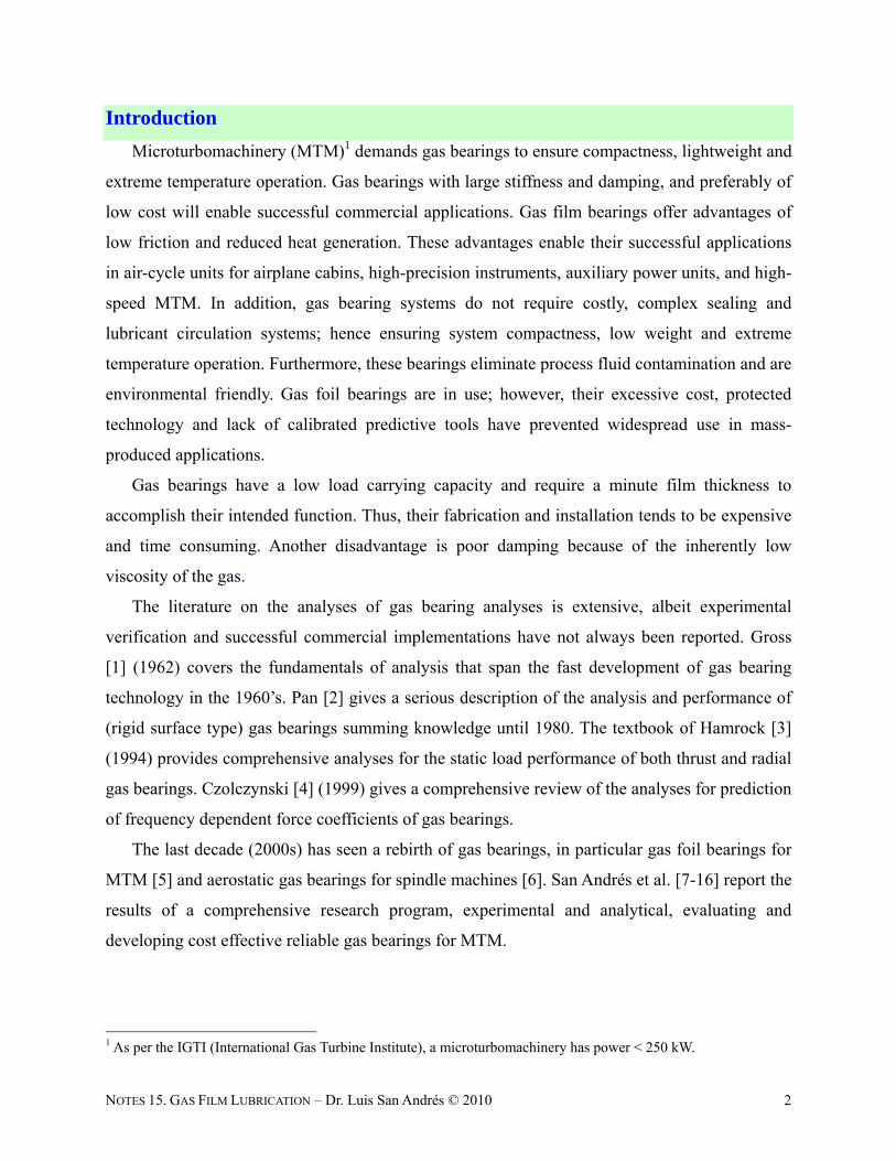
Introduction
Microturbomachinery (MTM)1 demands gas bearings to ensure compactness, lightweight and
extreme temperature operation. Gas bearings with large stiffness and damping, and preferably of
low cost will enable successful commercial applications. Gas film bearings offer advantages of
low friction and reduced heat generation. These advantages enable their successful applications
in air-cycle units for airplane cabins, high-precision instruments, auxiliary power units, and high-
speed MTM. In addition, gas bearing systems do not require costly, complex sealing and
lubricant circulation systems; hence ensuring system compactness, low weight and extreme
temperature operation. Furthermore, these bearings eliminate process fluid contamination and are
environmental friendly. Gas foil bearings are in use; however, their excessive cost, protected
technology and lack of calibrated predictive tools have prevented widespread use in mass-
produced applications.
Gas bearings have a low load carrying capacity and require a minute film thickness to
accomplish their intended function. Thus, their fabrication and installation tends to be expensive
and time consuming. Another disadvantage is poor damping because of the inherently low
viscosity of the gas.
The literature on the analyses of gas bearing analyses is extensive, albeit experimental
verification and successful commercial implementations have not always been reported. Gross
[1] (1962) covers the fundamentals of analysis that span the fast development of gas bearing
technology in the 1960’s. Pan [2] gives a serious description of the analysis and performance of
(rigid surface type) gas bearings summing knowledge until 1980. The textbook of Hamrock [3]
(1994) provides comprehensive analyses for the static load performance of both thrust and radial
gas bearings. Czolczynski [4] (1999) gives a comprehensive review of the analyses for prediction
of frequency dependent force coefficients of gas bearings.
The last decade (2000s) has seen a rebirth of gas bearings, in particular gas foil bearings for
MTM [5] and aerostatic gas bearings for spindle machines [6]. San Andrés et al. [7-16] report the
results of a comprehensive research program, experimental and analytical, evaluating and
developing cost effective reliable gas bearings for MTM.
1 As per the IGTI (International Gas Turbine Institute), a microturbomachinery has power < 250 kW.
NOTES 15. GAS FILM LUBRICATION – Dr. Luis San Andrés © 2010 3
Types of gas bearings
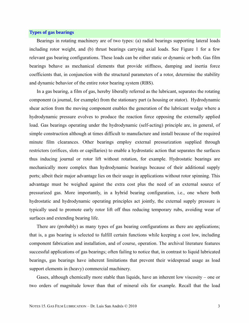
Bearings in rotating machinery are of two types: (a) radial bearings supporting lateral loads
including rotor weight, and (b) thrust bearings carrying axial loads. See Figure 1 for a few
relevant gas bearing configurations. These loads can be either static or dynamic or both. Gas film
bearings behave as mechanical elements that provide stiffness, damping and inertia force
coefficients that, in conjunction with the structural parameters of a rotor, determine the stability
and dynamic behavior of the entire rotor bearing system (RBS).
In a gas bearing, a film of gas, hereby liberally referred as the lubricant, separates the rotating
component (a journal, for example) from the stationary part (a housing or stator). Hydrodynamic
shear action from the moving component enables the generation of the lubricant wedge where a
hydrodynamic pressure evolves to produce the reaction force opposing the externally applied
load. Gas bearings operating under the hydrodynamic (self-acting) principle are, in general, of
simple construction although at times difficult to manufacture and install because of the required
minute film clearances. Other bearings employ external pressurization supplied through
restrictors (orifices, slots or capillaries) to enable a hydrostatic action that separates the surfaces
thus inducing journal or rotor lift without rotation, for example. Hydrostatic bearings are
mechanically more complex than hydrodynamic bearings because of their additional supply
ports; albeit their major advantage lies on their usage in applications without rotor spinning. This
advantage must be weighed against the extra cost plus the need of an external source of
pressurized gas. More importantly, in a hybrid bearing configuration, i.e., one where both
hydrostatic and hydrodynamic operating principles act jointly, the external supply pressure is
typically used to promote early rotor lift off thus reducing temporary rubs, avoiding wear of
surfaces and extending bearing life.
There are (probably) as many types of gas bearing configurations as there are applications;
that is, a gas bearing is selected to fulfill certain functions while keeping a cost low, including
component fabrication and installation, and of course, operation. The archival literature features
successful applications of gas bearings; often failing to notice that, in contrast to liquid lubricated
bearings, gas bearings have inherent limitations that prevent their widespread usage as load
support elements in (heavy) commercial machinery.
Gases, although chemically more stable than liquids, have an inherent low viscosity – one or
two orders of magnitude lower than that of mineral oils for example. Recall that the load

NOTES 15. GAS FILM LUBRICATION – Dr. Luis San Andrés © 2010 4
carrying capacity (W) of a self-acting hydrodynamic film bearing is roughly proportional to
2min
AUh
[3] where is the lubricant viscosity, U is the surface speed, A is the area of action,
and hmin is the minimum film thickness. Hence, in order to achieve a desired load capacity, a gas
lubricated bearing replacing a similar size oil-lubricated bearing must operate at an exceedingly
high surface speed (U) or with a minute film thickness (h). That is, hydrodynamic gas bearings
are not intended for supporting rotating machinery that operates with relatively low surface
speeds or if the film clearance or gap is too large. Hence, the need for accurate manufacturing of
parts which increases both cost and makes installation complicated. Of course, externally
pressurized (aerostatic) gas bearings can be used efficiently to carry loads at low or even zero
surface speeds. However, aerostatic bearings require a source of pressurized gas which adds cost
and complexity [1,6,10].
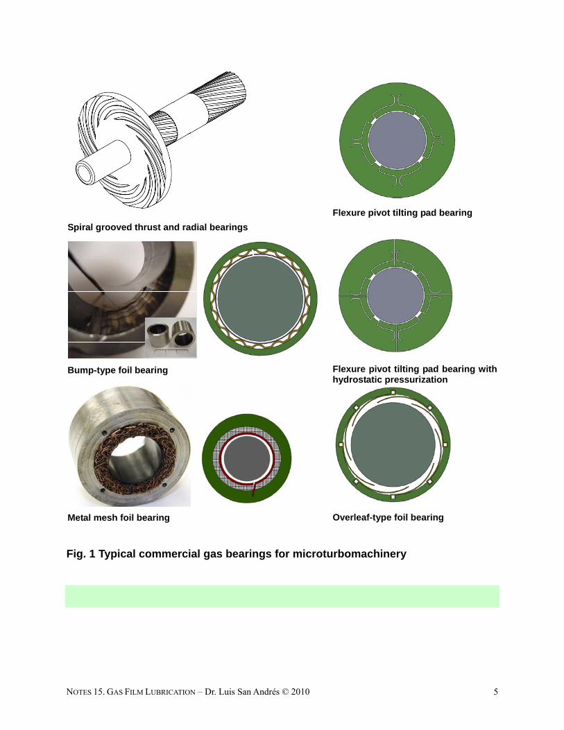
To enhance the hydrodynamic action, designers have produced a number of bearing
configurations that exploit geometrical features such as steps, grooves, pockets and dimples, for
example. Figure 1 shows several typical commercial gas bearing configurations. The bearing
types with textured surfaces, known as (spiral) grooved bearings and herringbone journal
bearings have been instrumental to the operation of gyroscopes for aircraft and satellite
navigation [2], enabled non contacting gas face seal technology [7]; and more recently, allowed
the revolution in digital storage hard-drive technology [17]. In these applications, static and
dynamics loads are relatively low. Note that, for optimum load performance giving the maximum
static (centering) stiffness, the depth of the machined steps or grooves or pockets is just equal or
a little larger than the operating film gap or clearance, as will be demonstrated later. Until
recently, these geometrical features were difficult to machine at low cost, except in certain
materials like silicon-carbide for non-contacting face seals. However, current casting and
manufacturing processes allow the manufacturing of these bearings (or seals) at a relatively low
cost and with near identical performance in one or millions of pieces.
Other radial bearing configurations of interest, i.e., undergoing close scrutiny and
commercial development, include bump-type foil bearings [5, 15, 18], flexure pivot tilting pad
bearings [13], and (low cost) metal mesh foil bearings [19].
NOTES 15. GAS FILM LUBRICATION – Dr. Luis San Andrés © 2010 5
Spiral grooved thrust and radial bearings
Flexure pivot tilting pad bearing
Bump-type foil bearing
Flexure pivot tilting pad bearing with hydrostatic pressurization
Metal mesh foil bearing
Overleaf-type foil bearing
Fig. 1 Typical commercial gas bearings for microturbomachinery
NOTES 15. GAS FILM LUBRICATION – Dr. Luis San Andrés © 2010 6
The fundamentals of gas film lubrication analysis
The fluid flow in a hydrodynamic gas bearing or gas face seal is typically laminar and
inertialess, i.e. the Reynolds numbers Re=Uh/ <1, because of the smallness in film thickness
(h) and the low lubricant density (). Gas annular seals, such as labyrinth and honeycomb types,
are notable exceptions, since in these applications large pressure drops, high surface speeds and
large clearances promote flow turbulence accompanied by strong fluid compressibility effects
[20].
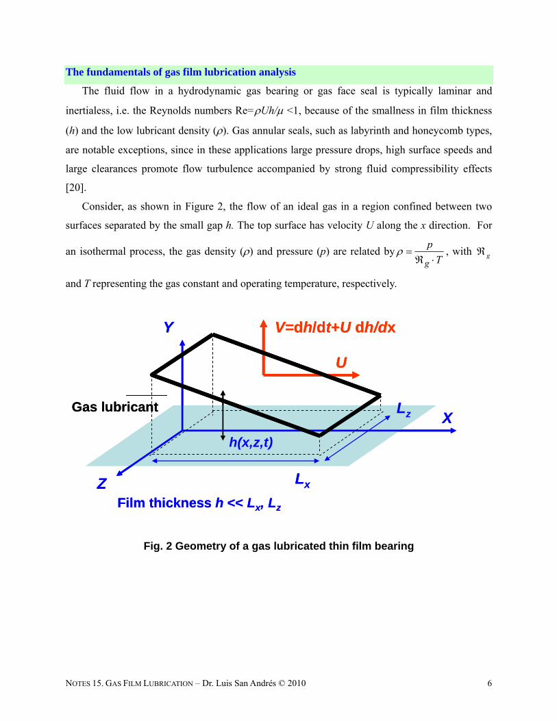
Consider, as shown in Figure 2, the flow of an ideal gas in a region confined between two
surfaces separated by the small gap h. The top surface has velocity U along the x direction. For
an isothermal process, the gas density () and pressure (p) are related byg
p
T
, with g
and T representing the gas constant and operating temperature, respectively.
Gas lubricantX
Y
Z
U
V=dh/dt+U dh/dx
Lx
Lz
h(x,z,t)
Film thickness h << Lx, Lz
Gas lubricantX
Y
Z
U
V=dh/dt+U dh/dx
Lx
Lz
h(x,z,t)
Film thickness h << Lx, Lz
Fig. 2 Geometry of a gas lubricated thin film bearing
NOTES 15. GAS FILM LUBRICATION – Dr. Luis San Andrés © 2010 7
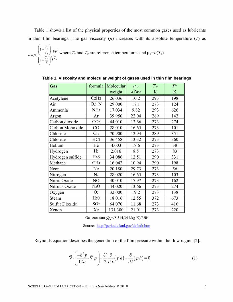
Table 1 shows a list of the physical properties of the most common gases used as lubricants
in thin film bearings. The gas viscosity () increases with its absolute temperature (T) as
*
0
*
1
1o
o
T
T TT TT
where T* and To are reference temperatures and o=(To).
Table 1. Viscosity and molecular weight of gases used in thin film bearings
Gas formula Molecular T o T*weight Pa-s K K
Acetylene C2H2 26.036 10.2 293 198Air O2+N 29.000 17.1 273 124Ammonia NH3 17.034 9.82 293 626Argon Ar 39.950 22.04 289 142Carbon dioxide CO2 44.010 13.66 273 274Carbon Monoxide CO 28.010 16.65 273 101Chlorine Cl2 70.900 12.94 289 351Chloride HCl 36.458 13.32 273 360Helium He 4.003 18.6 273 38Hydrogen H2 2.016 8.5 273 83Hydrogen sulfide H2S 34.086 12.51 290 331Methane CH4 16.042 10.94 290 198Neon Ne 20.180 29.73 273 56Nitrogen N2 28.020 16.65 273 103Nitric Oxide NO 30.010 17.97 273 162Nitrous Oxide N2O 44.020 13.66 273 274Oxygen O2 32.000 19.2 273 138Steam H20 18.016 12.55 372 673Sulfur Dioxide SO2 64.070 11.68 273 416Xenon Xe 131.300 21.01 273 220
Gas constant Rg=(8,314,34 J/kg-K)/MW
Source: http://periodic.lanl.gov/default.htm
Reynolds equation describes the generation of the film pressure within the flow region [2].
3
012 2
h p Up p h p h
x t
(1)
NOTES 15. GAS FILM LUBRICATION – Dr. Luis San Andrés © 2010 8
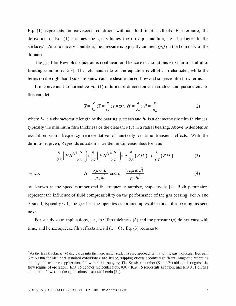
Eq. (1) represents an isoviscous condition without fluid inertia effects. Furthermore, the
derivation of Eq. (1) assumes the gas satisfies the no-slip condition, i.e. it adheres to the
surfaces2. As a boundary condition, the pressure is typically ambient (pa) on the boundary of the
domain.
The gas film Reynolds equation is nonlinear; and hence exact solutions exist for a handful of
limiting conditions [2,3]. The left hand side of the equation is elliptic in character, while the
terms on the right hand side are known as the shear induced flow and squeeze film flow terms.
It is convenient to normalize Eq. (1) in terms of dimensionless variables and parameters. To
this end, let
* * *; ; ; ;
a
x z h px z t H P
L L h p (2)
where L* is a characteristic length of the bearing surfaces and h* is a characteristic film thickness;
typically the minimum film thickness or the clearance (c) in a radial bearing. Above denotes an
excitation whirl frequency representative of unsteady or time transient effects. With the
definitions given, Reynolds equation is written in dimensionless form as
3 3P PP H P H P H P H
x x z z x
(3)
where 2
* *2 2* *
6 12and
a a
U L L
p h p h
(4)
are known as the speed number and the frequency number, respectively [2]. Both parameters
represent the influence of fluid compressibility on the performance of the gas bearing. For and
small, typically < 1, the gas bearing operates as an incompressible fluid film bearing, as seen
next.
For steady state applications, i.e., the film thickness (h) and the pressure (p) do not vary with
time, and hence squeeze film effects are nil (Eq. (3) reduces to
2 As the film thickness (h) decreases into the nano meter scale, its size approaches that of the gas molecular free path (= 60 nm for air under standard conditions); and hence, slipping effects become significant. Magnetic recording and digital hard drive applications fall within this category. The Knudsen number (Kn=/h ) aids to distinguish the flow regime of operation; Kn> 15 denotes molecular flow, 0.01< Kn< 15 represents slip flow, and Kn<0.01 gives a continuum flow, as in the applications discussed herein [21].
NOTES 15. GAS FILM LUBRICATION – Dr. Luis San Andrés © 2010 9
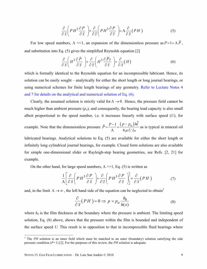
3 3P PP H P H P H
x x z z x
(5)
For low speed numbers, <<1, an expansion of the dimensionless pressure as 1P P ,
and substitution into Eq. (5) gives the simplified Reynolds equation [2]
3 3 )P PH H H
x x z z x
(6)
which is formally identical to the Reynolds equation for an incompressible lubricant. Hence, its
solution can be easily sought – analytically for either the short length or long journal bearings, or
using numerical schemes for finite length bearings of any geometry. Refer to Lecture Notes 4
and 7 for details on the analytical and numerical solution of Eq. (6).
Clearly, the assumed solution is strictly valid for 0 . Hence, the pressure field cannot be
much higher than ambient pressure (pa), and consequently, the bearing load capacity is also small
albeit proportional to the speed number, i.e. it increases linearly with surface speed (U), for
example. Note that the dimensionless pressure 2
*
*
1
6ap p hP
PU L
as is typical in mineral oil
lubricated bearings. Analytical solutions to Eq. (5) are available for either the short length or
infinitely long cylindrical journal bearings, for example. Closed form solutions are also available
for simple one-dimensional slider or Rayleigh-step bearing geometries, see Refs. [2, 21] for
example.
On the other hand, for large speed numbers, >>1, Eq. (5) is written as
3 31 P PP H P H P H
x x z z x
(7)
and, in the limit , the left hand side of the equation can be neglected to obtain3
0( )b
ah
P H p px h x
(8)
where hb is the film thickness at the boundary where the pressure is ambient. The limiting speed
solution, Eq. (8) above, shows that the pressure within the film is bounded and independent of
the surface speed U. This result is in opposition to that in incompressible fluid bearings where
3 The PH solution is an inner field which must be matched to an outer (boundary) solution satisfying the side pressure condition (P=1) [2]. For the purposes of this review, the PH solution is adequate.
NOTES 15. GAS FILM LUBRICATION – Dr. Luis San Andrés © 2010 10
the generated hydrodynamic film pressure is proportional to the surface speed U. Since the
pressure has a definite limit, it also means that the bearing load capacity has also a limit, i.e. an
ultimate value. In this regard, gas film bearings do show a significant difference with
incompressible fluid (mineral oil lubricated) bearings whose (theoretical) load capacity increases
with surface speed.
Closed form solutions for finite speed numbers () are not readily available. Hence,
predictions of bearing film pressure and its force reaction supporting an applied load must rely
on numerical analysis. For low to moderate speed numbers, finite differences or finite element
methods applicable to elliptical differential equations are quite adequate. However, it is well
known that these numerical methods are inaccurate and numerically unstable for large speed
numbers () since the nature of the Reynolds equation evolves from a (second order) elliptical
form into a (first order) parabolic form. See Ref. [8] for a significant advance that resolves the
issue of pressure oscillations and numerical instability for large speed numbers ()
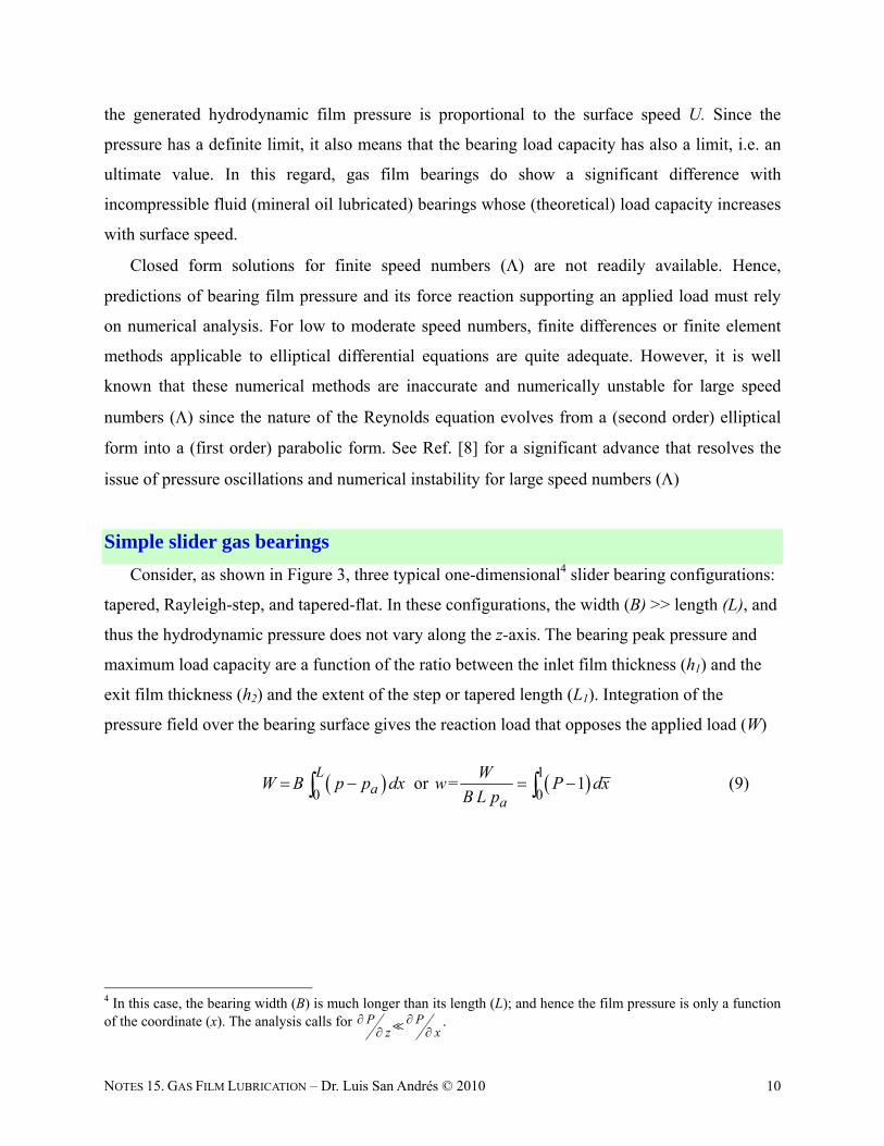
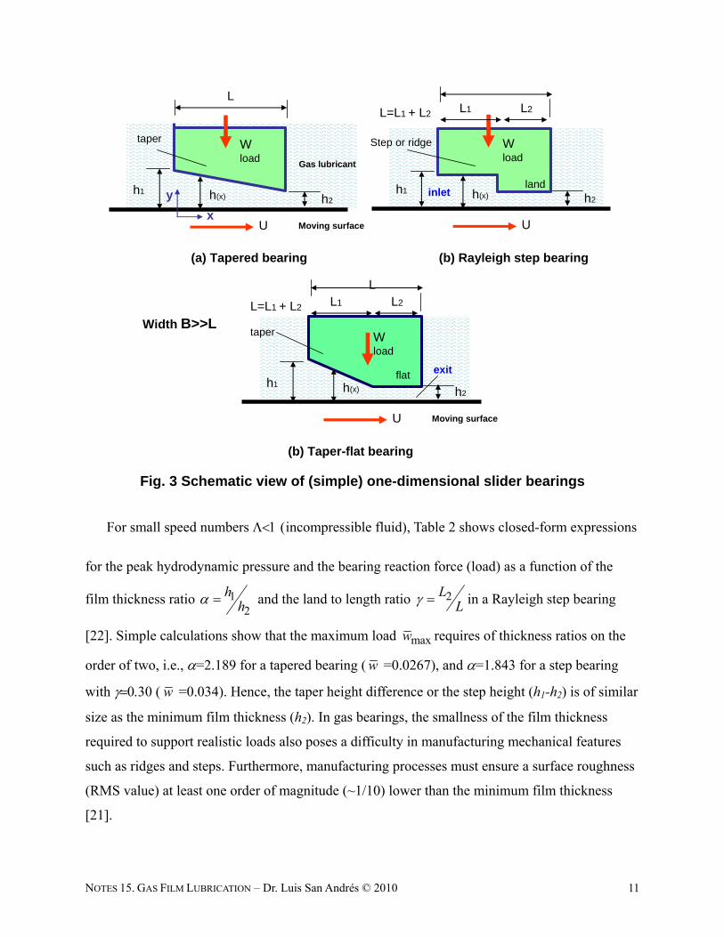
Simple slider gas bearings
Consider, as shown in Figure 3, three typical one-dimensional4 slider bearing configurations:
tapered, Rayleigh-step, and tapered-flat. In these configurations, the width (B) >> length (L), and
thus the hydrodynamic pressure does not vary along the z-axis. The bearing peak pressure and
maximum load capacity are a function of the ratio between the inlet film thickness (h1) and the
exit film thickness (h2) and the extent of the step or tapered length (L1). Integration of the
pressure field over the bearing surface gives the reaction load that opposes the applied load (W)
1
0 0or = 1
La
a
WW B p p dx w P dx
B L p (9)
4 In this case, the bearing width (B) is much longer than its length (L); and hence the film pressure is only a function of the coordinate (x). The analysis calls for P P
z x
.
NOTES 15. GAS FILM LUBRICATION – Dr. Luis San Andrés © 2010 11
U
Wload
h1h2h(x)
L
x
y
(a) Tapered bearing
Gas lubricant
Moving surface U
Wload
h1h2h(x)
Width B>>L
L1 L2L=L1 + L2
Step or ridge
land
(b) Rayleigh step bearing
U
Wload
h1h2h(x)
L
Moving surface
L1 L2L=L1 + L2
taper
flat
(b) Taper-flat bearing
taper
inlet
exit
Fig. 3 Schematic view of (simple) one-dimensional slider bearings
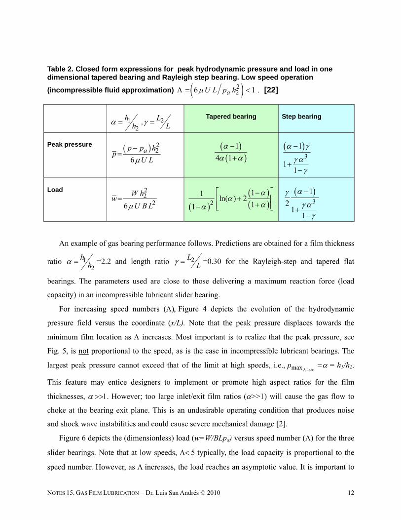
For small speed numbers incompressible fluid, Table 2 shows closed-form expressions
for the peak hydrodynamic pressure and the bearing reaction force (load) as a function of the
film thickness ratio 12
hh and the land to length ratio 2L
L in a Rayleigh step bearing
[22]. Simple calculations show that the maximum load maxw requires of thickness ratios on the
order of two, i.e., =2.189 for a tapered bearing ( w =0.0267), and =1.843 for a step bearing
with w =0.034). Hence, the taper height difference or the step height (h1-h2) is of similar
size as the minimum film thickness (h2). In gas bearings, the smallness of the film thickness
required to support realistic loads also poses a difficulty in manufacturing mechanical features
such as ridges and steps. Furthermore, manufacturing processes must ensure a surface roughness
(RMS value) at least one order of magnitude (~1/10) lower than the minimum film thickness
[21].
NOTES 15. GAS FILM LUBRICATION – Dr. Luis San Andrés © 2010 12
Table 2. Closed form expressions for peak hydrodynamic pressure and load in one dimensional tapered bearing and Rayleigh step bearing. Low speed operation
(incompressible fluid approximation) 226 aU L p h [22]
An example of gas bearing performance follows. Predictions are obtained for a film thickness
ratio 12
hh =2.2 and length ratio 2L
L =0.30 for the Rayleigh-step and tapered flat
bearings. The parameters used are close to those delivering a maximum reaction force (load
capacity) in an incompressible lubricant slider bearing.
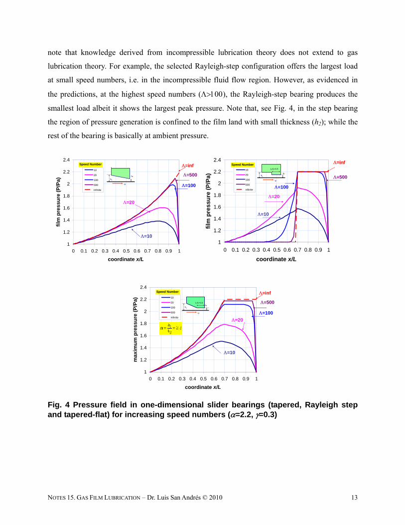
For increasing speed numbers (Figure 4 depicts the evolution of the hydrodynamic
pressure field versus the coordinate (x/L). Note that the peak pressure displaces towards the
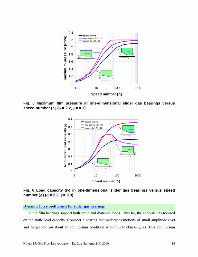
minimum film location as increases. Most important is to realize that the peak pressure, see
Fig. 5, is not proportional to the speed, as is the case in incompressible lubricant bearings. The
largest peak pressure cannot exceed that of the limit at high speeds, i.e., maxp
= h1/h2.
This feature may entice designers to implement or promote high aspect ratios for the film
thicknesses, However; too large inlet/exit film ratios (>>1) will cause the gas flow to
choke at the bearing exit plane. This is an undesirable operating condition that produces noise
and shock wave instabilities and could cause severe mechanical damage [2].
Figure 6 depicts the (dimensionless) load (w=W/BLpa) versus speed number () for the three
slider bearings. Note that at low speeds, typicallythe load capacity is proportional to the
speed number. However, as increases, the load reaches an asymptotic value. It is important to
1
2
hh , 2L
L Tapered bearing Step bearing
Peak pressure
22
6ap p h
pU L
1
4 1
3
1
11
Load
22
26
W hw
U B L
2
11ln( ) 2
11
3
1
21
1
NOTES 15. GAS FILM LUBRICATION – Dr. Luis San Andrés © 2010 13
note that knowledge derived from incompressible lubrication theory does not extend to gas
lubrication theory. For example, the selected Rayleigh-step configuration offers the largest load
at small speed numbers, i.e. in the incompressible fluid flow region. However, as evidenced in
the predictions, at the highest speed numbers (), the Rayleigh-step bearing produces the
smallest load albeit it shows the largest peak pressure. Note that, see Fig. 4, in the step bearing
the region of pressure generation is confined to the film land with small thickness (h2); while the
rest of the bearing is basically at ambient pressure.
1
1.2
1.4
1.6
1.8
2
2.2
2.4
0 0.1 0.2 0.3 0.4 0.5 0.6 0.7 0.8 0.9 1
coordinate x/L
film
pre
ssu
re (
P/P
a)
10
20
100
500
infinite
Speed Number
=10
=20
=100
=500
=inf
h2
U
h1
1
1.2
1.4
1.6
1.8
2
2.2
2.4
0 0.1 0.2 0.3 0.4 0.5 0.6 0.7 0.8 0.9 1
coordinate x/L
film
pre
ssu
re (
P/P
a)
10
20
100
500
infinite
Speed Number
=10
=20
=100
=500
=inf
h2
h1
U
L2/L=0.3
1
1.2
1.4
1.6
1.8
2
2.2
2.4
0 0.1 0.2 0.3 0.4 0.5 0.6 0.7 0.8 0.9 1
coordinate x/L
ma
xim
um
pre
ssu
re (
P/P
a)
10
20
100
500
infinite
Speed Number
=10
=20
=100
=500
=inf
h2h1
U
L2/L=0.3
Fig. 4 Pressure field in one-dimensional slider bearings (tapered, Rayleigh step and tapered-flat) for increasing speed numbers (=2.2, =0.3)
NOTES 15. GAS FILM LUBRICATION – Dr. Luis San Andrés © 2010 14
1
1.2
1.4
1.6
1.8
2
2.2
2.4
1 10 100 1000
Speed number ()
max
imu
m p
ress
ure
(P
/Pa)
tapered bearingStep bearing L2/L=0.3tapered flat L2/L=0.3
h2
U
h1
h2
h1
U
L2/L=0.3 h2h1
U
L2/L=0.3
Fig. 5 Maximum film pressure in one-dimensional slider gas bearings versus speed number ( (= 2.2, = 0.3)
0
0.1
0.2
0.3
0.4
0.5
0.6
0.7
1 10 100 1000
Speed number ()
No
rmal
ized
lo
ad c
apac
ity
[-]
tapered bearing
step bearing L2/L=0.3
tapered flat L2/L=0.3
h2
U
h1
h2
h1
U
L2/L=0.3
h2h1
U
L2/L=0.3
Fig. 6 Load capacity (w) in one-dimensional slider gas bearings versus speed number ( (= 2.2, = 0.3)
Dynamic force coefficients for slider gas bearings
Fluid film bearings support both static and dynamic loads. Thus far, the analysis has focused
on the static load capacity. Consider a bearing that undergoes motions of small amplitude (y)
and frequency () about an equilibrium condition with film thickness ho(x). This equilibrium
NOTES 15. GAS FILM LUBRICATION – Dr. Luis San Andrés © 2010 15
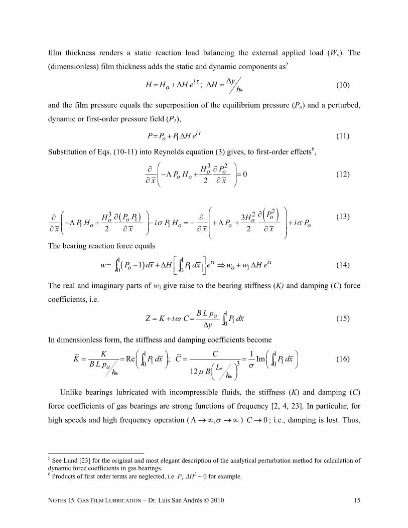
film thickness renders a static reaction load balancing the external applied load (Wo). The
(dimensionless) film thickness adds the static and dynamic components as5
*;i
oyH H H e H h
(10)
and the film pressure equals the superposition of the equilibrium pressure (Po) and a perturbed,
dynamic or first-order pressure field (P1),
1i
oP P P H e (11)
Substitution of Eqs. (10-11) into Reynolds equation (3) gives, to first-order effects6,
3 20
2o o
o oH P
P Hx x
(12)
23 21
1 13
2 2
ooo oo o o o
PP PH HP H i P H P i P
x x x x
(13)
The bearing reaction force equals
1 11 10 0
1 i io ow P dx H P dx e w w H e (14)
The real and imaginary parts of w1 give raise to the bearing stiffness (K) and damping (C) force
coefficients, i.e.
110
aB L pZ K i C P dx
y
(15)
In dimensionless form, the stiffness and damping coefficients become
1 11 130 0
** *
1Re ; Im
12a
K CK P dx C P dx
B L p LBh h
(16)
Unlike bearings lubricated with incompressible fluids, the stiffness (K) and damping (C)
force coefficients of gas bearings are strong functions of frequency [2, 4, 23]. In particular, for
high speeds and high frequency operation ( , ) 0C ; i.e., damping is lost. Thus,
5 See Lund [23] for the original and most elegant description of the analytical perturbation method for calculation of dynamic force coefficients in gas bearings. 6 Products of first order terms are neglected, i.e. P1 H2 ~ 0 for example.
NOTES 15. GAS FILM LUBRICATION – Dr. Luis San Andrés © 2010 16
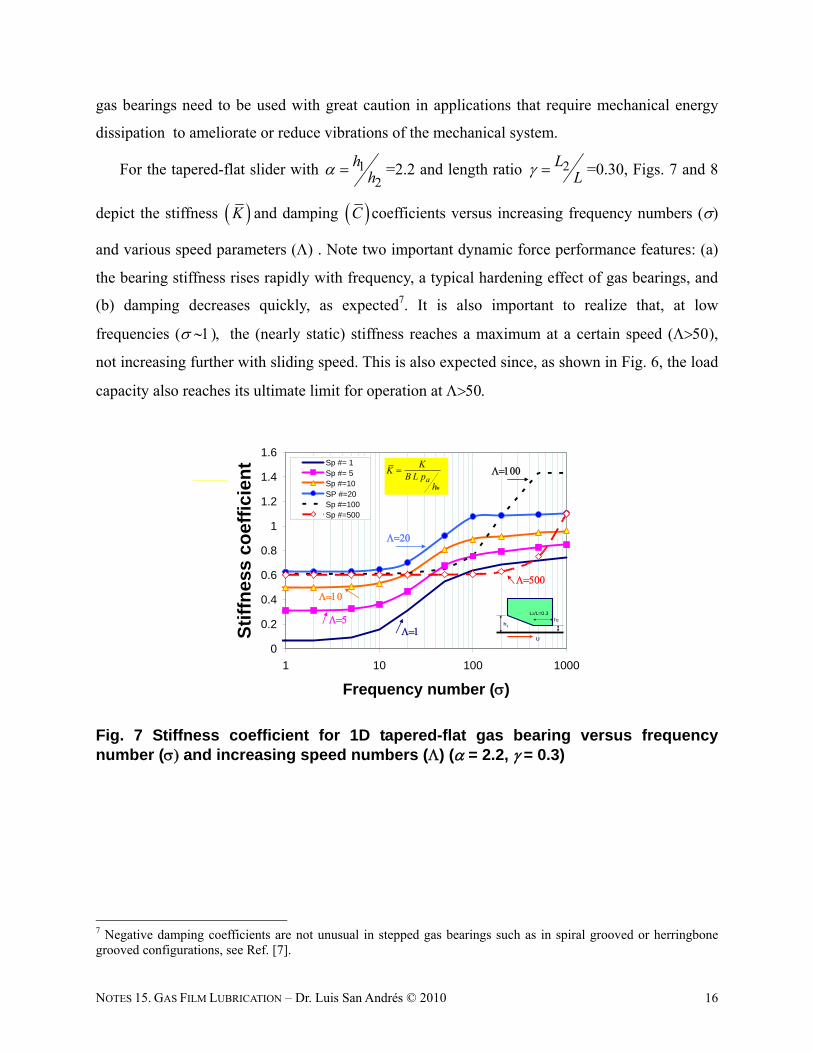
gas bearings need to be used with great caution in applications that require mechanical energy
dissipation to ameliorate or reduce vibrations of the mechanical system.
For the tapered-flat slider with 12
hh =2.2 and length ratio 2L
L =0.30, Figs. 7 and 8
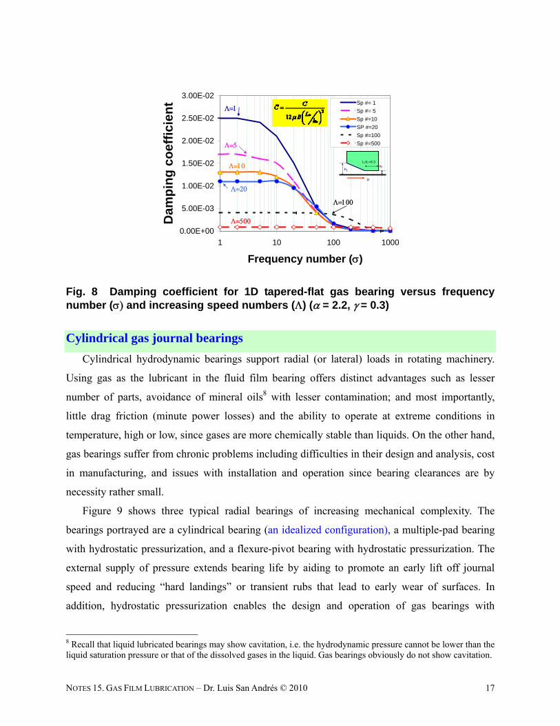
depict the stiffness K and damping C coefficients versus increasing frequency numbers ()
and various speed parameters () . Note two important dynamic force performance features: (a)
the bearing stiffness rises rapidly with frequency, a typical hardening effect of gas bearings, and
(b) damping decreases quickly, as expected7. It is also important to realize that, at low
frequencies ( the (nearly static) stiffness reaches a maximum at a certain speed (),
not increasing further with sliding speed. This is also expected since, as shown in Fig. 6, the load
capacity also reaches its ultimate limit for operation at
0
0.2
0.4
0.6
0.8
1
1.2
1.4
1.6
1 10 100 1000
Frequency number ()
Sti
ffn
ess
coef
fici
ent Sp #= 1
Sp #= 5Sp #=10SP #=20Sp #=100Sp #=500
h2h1
U
L2/L=0.3
*a
KK
B L ph
Fig. 7 Stiffness coefficient for 1D tapered-flat gas bearing versus frequency number ( and increasing speed numbers () (= 2.2, = 0.3)
7 Negative damping coefficients are not unusual in stepped gas bearings such as in spiral grooved or herringbone grooved configurations, see Ref. [7].
NOTES 15. GAS FILM LUBRICATION – Dr. Luis San Andrés © 2010 17
0.00E+00
5.00E-03
1.00E-02
1.50E-02
2.00E-02
2.50E-02
3.00E-02
1 10 100 1000
Frequency number ()
Dam
pin
g c
oef
fici
ent Sp #= 1
Sp #= 5
Sp #=10
SP #=20
Sp #=100
Sp #=500
h2h1
U
L2/L=0.3
Fig. 8 Damping coefficient for 1D tapered-flat gas bearing versus frequency number ( and increasing speed numbers () (= 2.2, = 0.3)
Cylindrical gas journal bearings
Cylindrical hydrodynamic bearings support radial (or lateral) loads in rotating machinery.
Using gas as the lubricant in the fluid film bearing offers distinct advantages such as lesser
number of parts, avoidance of mineral oils8 with lesser contamination; and most importantly,
little drag friction (minute power losses) and the ability to operate at extreme conditions in
temperature, high or low, since gases are more chemically stable than liquids. On the other hand,
gas bearings suffer from chronic problems including difficulties in their design and analysis, cost
in manufacturing, and issues with installation and operation since bearing clearances are by
necessity rather small.
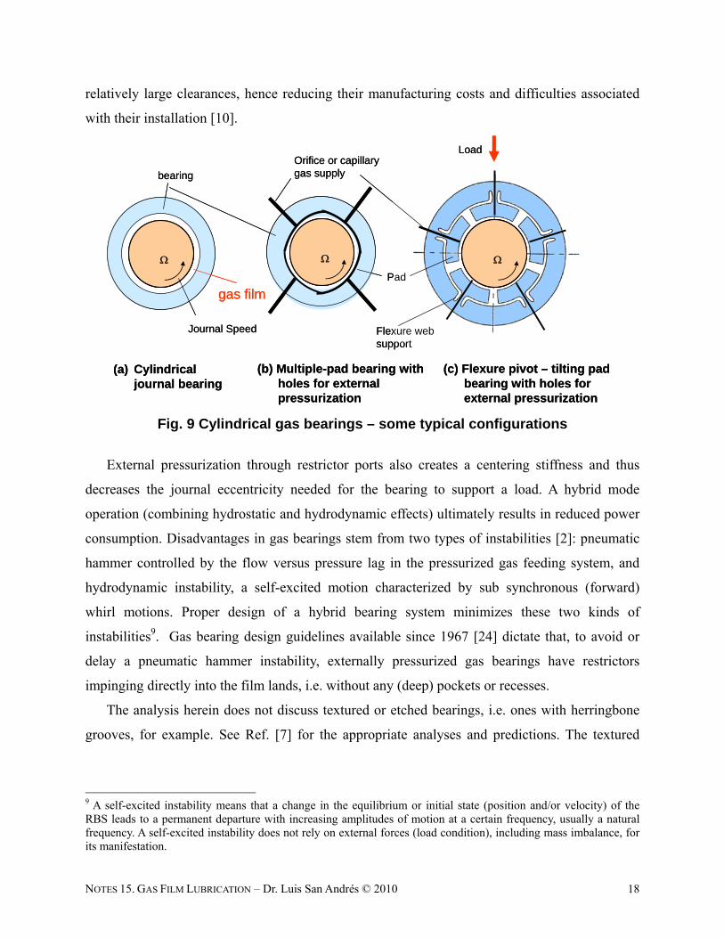
Figure 9 shows three typical radial bearings of increasing mechanical complexity. The
bearings portrayed are a cylindrical bearing (an idealized configuration), a multiple-pad bearing
with hydrostatic pressurization, and a flexure-pivot bearing with hydrostatic pressurization. The
external supply of pressure extends bearing life by aiding to promote an early lift off journal
speed and reducing “hard landings” or transient rubs that lead to early wear of surfaces. In
addition, hydrostatic pressurization enables the design and operation of gas bearings with
8 Recall that liquid lubricated bearings may show cavitation, i.e. the hydrodynamic pressure cannot be lower than the liquid saturation pressure or that of the dissolved gases in the liquid. Gas bearings obviously do not show cavitation.
NOTES 15. GAS FILM LUBRICATION – Dr. Luis San Andrés © 2010 18
relatively large clearances, hence reducing their manufacturing costs and difficulties associated
with their installation [10].
Flexure web support
Journal Speed
bearing
Orifice or capillarygas supply
Pad
gas film
Load
(a) Cylindrical journal bearing
(b) Multiple-pad bearing with holes for external pressurization
(c) Flexure pivot – tilting pad bearing with holes for external pressurization
Flexure web support
Journal Speed
bearing
Orifice or capillarygas supply
Pad
gas film
Load
(a) Cylindrical journal bearing
(b) Multiple-pad bearing with holes for external pressurization
(c) Flexure pivot – tilting pad bearing with holes for external pressurization
Fig. 9 Cylindrical gas bearings – some typical configurations
External pressurization through restrictor ports also creates a centering stiffness and thus
decreases the journal eccentricity needed for the bearing to support a load. A hybrid mode
operation (combining hydrostatic and hydrodynamic effects) ultimately results in reduced power
consumption. Disadvantages in gas bearings stem from two types of instabilities [2]: pneumatic
hammer controlled by the flow versus pressure lag in the pressurized gas feeding system, and
hydrodynamic instability, a self-excited motion characterized by sub synchronous (forward)
whirl motions. Proper design of a hybrid bearing system minimizes these two kinds of
instabilities9. Gas bearing design guidelines available since 1967 [24] dictate that, to avoid or
delay a pneumatic hammer instability, externally pressurized gas bearings have restrictors
impinging directly into the film lands, i.e. without any (deep) pockets or recesses.
The analysis herein does not discuss textured or etched bearings, i.e. ones with herringbone
grooves, for example. See Ref. [7] for the appropriate analyses and predictions. The textured
9 A self-excited instability means that a change in the equilibrium or initial state (position and/or velocity) of the RBS leads to a permanent departure with increasing amplitudes of motion at a certain frequency, usually a natural frequency. A self-excited instability does not rely on external forces (load condition), including mass imbalance, for its manifestation.
NOTES 15. GAS FILM LUBRICATION – Dr. Luis San Andrés © 2010 19
bearings are still costly to manufacture, offer little improvements in load capacity, and have
severe limitations in terms of rotordynamic stability [12].
For certain static load dispositions, tilting pad bearings can eliminate the typically harmful
hydrodynamic instability by not generating cross-coupled stiffness coefficients. Critical
turbomachinery operating well above its critical speeds is customarily implemented with tilting
pad bearings. The multiplicity of parameters associated with a tilting pad bearing demands
complex analytical methods for predictions of force coefficients and stability calculations [10].
Incidentally, conventional (commercial) tilting pad bearings cannot be easily modified to add
external pressurization (holes through pivots and pads) without constraining severely the pads’
motion and adding sealing issues.
The flexure pivot – tilting pad bearing (FPTPB), see Fig. 9, offers a marked improvement
over the conventional design since its wire discharge machining (EDM) construction renders an
integral pads-bearing configuration, thus eliminating pivot wear and stack up of tolerances on
assembly [13]. Each pad connects to the bearing through a thin flexural web, which provides a
low rotational stiffness, thus ensuring small cross-coupled stiffness coefficients and avoiding
subsynchronous instabilities into very high speed operation.
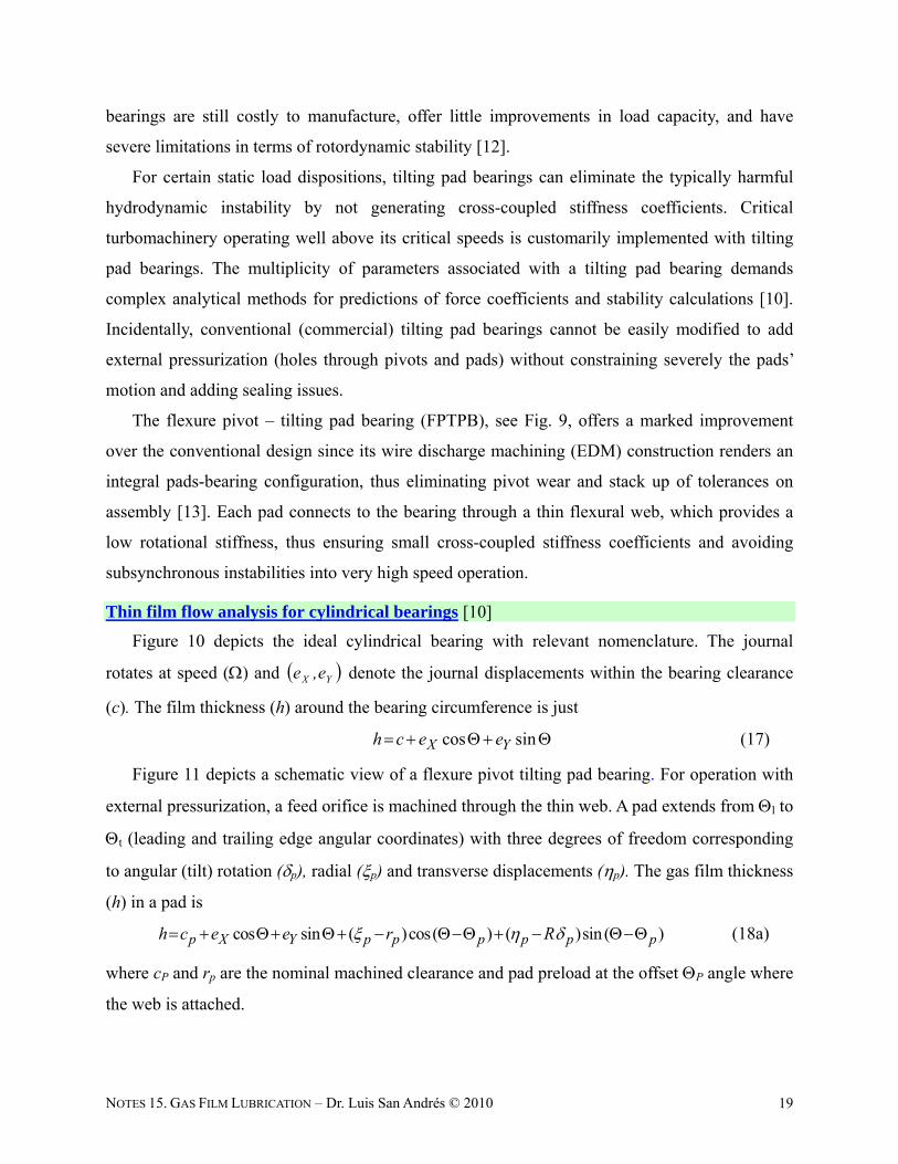
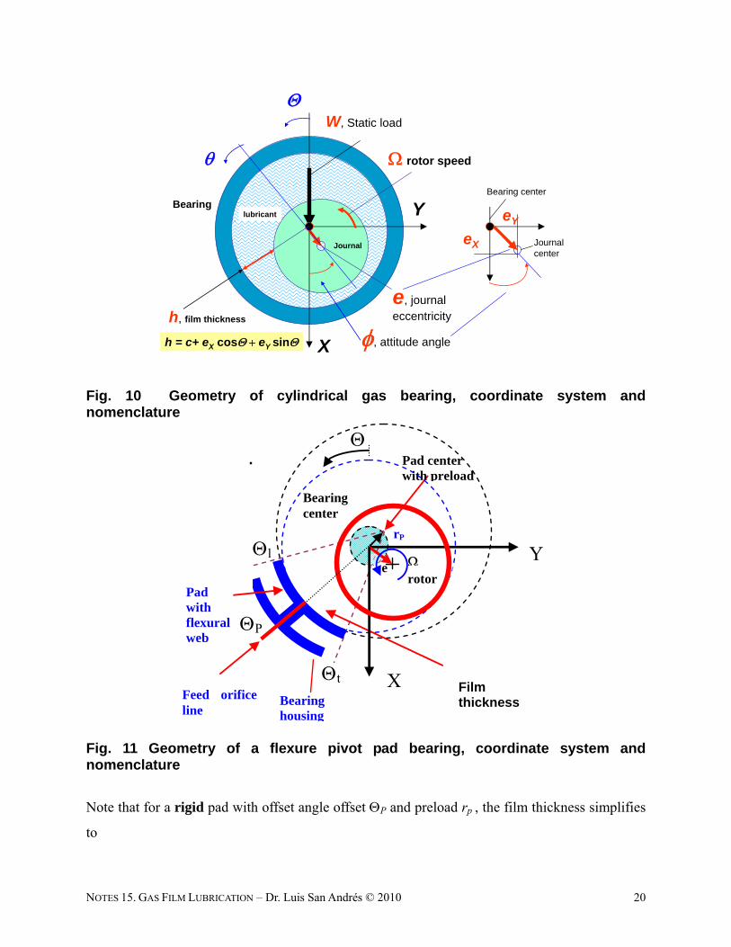
Thin film flow analysis for cylindrical bearings [10]
Figure 10 depicts the ideal cylindrical bearing with relevant nomenclature. The journal
rotates at speed () and YX e,e denote the journal displacements within the bearing clearance
(c). The film thickness (h) around the bearing circumference is just
cos sinX Yh c e e (17)
Figure 11 depicts a schematic view of a flexure pivot tilting pad bearing. For operation with
external pressurization, a feed orifice is machined through the thin web. A pad extends from l to
t (leading and trailing edge angular coordinates) with three degrees of freedom corresponding
to angular (tilt) rotation (p), radial (p) and transverse displacements (p). The gas film thickness
(h) in a pad is
cos sin ( )cos( ) ( )sin ( )p X Y p p p p p ph c e e r R (18a)
where cP and rp are the nominal machined clearance and pad preload at the offset P angle where
the web is attached.
NOTES 15. GAS FILM LUBRICATION – Dr. Luis San Andrés © 2010 20
X
Y
rotor speed
Journal
Bearing
W, Static load
e, journal eccentricity
, attitude angle
lubricant
Bearing center
h, film thickness
eX
eY
Journal center
h = c+ eX cos eY sin
Fig. 10 Geometry of cylindrical gas bearing, coordinate system and nomenclature
Pad with flexural web
l
P
t X
Y
e
Pad center with preload
Bearing center
Bearing housing
Film thickness
rotor
Feed orifice line
rP
Fig. 11 Geometry of a flexure pivot pad bearing, coordinate system and nomenclature
Note that for a rigid pad with offset angle offset P and preload rp , the film thickness simplifies
to
NOTES 15. GAS FILM LUBRICATION – Dr. Luis San Andrés © 2010 21
cos cos sinp p X Yh c r e e (18b)
In a radial bearing, Reynolds equation for the laminar flow of an ideal gas and under
isothermal conditions governs the generation of hydrodynamic pressure within the thin film
region, i.e., [2]
3
12 2 OR gh p
p p h p h m Tt
(19)
where ORm denotes mass flow through a supply port at pressure pS . The pressure is ambient (pa)
on the sides (z=0, L) of a bearing pad.
For an inherent restrictor, the flow rate is a function of the pressure ratio orS
pP p , the
orifice diameter (d) and the local film thickness (h), i.e. from [24],
( )SOR
g
pm d h P
T
(20)
with
1 12 1 1
1 12 1 1 2
2 22
1 1 1
2 11
choke
choke
for P P
P
P P for P P
(21)
where κ is the gas specific heats ratio. The orifice restriction is of inherent type10 whose flow is
strongly affected by the local film thickness.
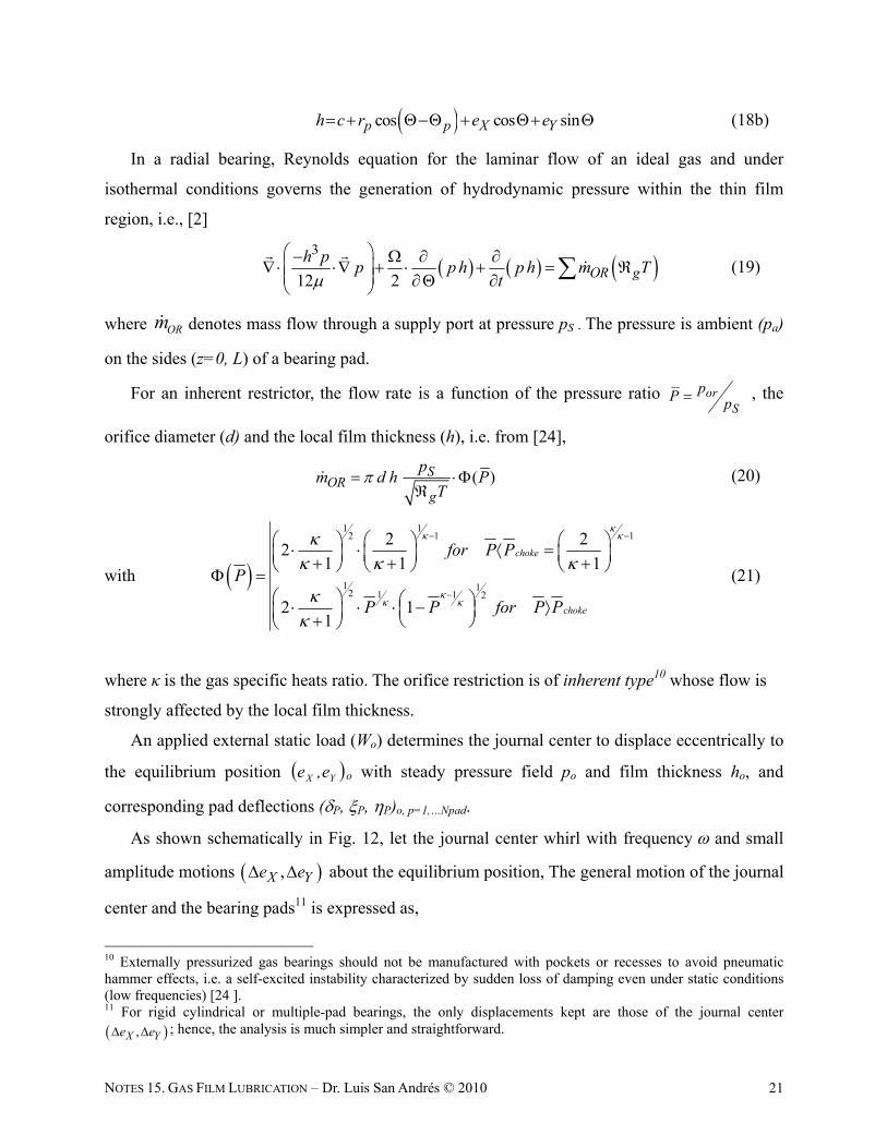
An applied external static load (Wo) determines the journal center to displace eccentrically to
the equilibrium position YX e,e o with steady pressure field po and film thickness ho, and
corresponding pad deflections (P, P, P)o, p=1,…Npad.
As shown schematically in Fig. 12, let the journal center whirl with frequency and small
amplitude motions ,X Ye e about the equilibrium position, The general motion of the journal
center and the bearing pads11 is expressed as,
10 Externally pressurized gas bearings should not be manufactured with pockets or recesses to avoid pneumatic hammer effects, i.e. a self-excited instability characterized by sudden loss of damping even under static conditions (low frequencies) [24 ]. 11 For rigid cylindrical or multiple-pad bearings, the only displacements kept are those of the journal center
,X Ye e ; hence, the analysis is much simpler and straightforward.
NOTES 15. GAS FILM LUBRICATION – Dr. Luis San Andrés © 2010 22
,i tX Xo Xe e e e ,i t
Y Yo Ye e e e
,i tp po p e ,i t
p po p e i tp po p e p = 1,2,...,Npad (22)
with 1i . The film thickness and hydrodynamic pressure are also given by the superposition
of equilibrium (zeroth order) and perturbed (first-order) fields, i.e.
i toh h h e ; i t
op p pe (23)
where
cos sin cos( ) sin ( )X Y P P P P Ph e e R (24)
and X X Y Y P P Pp p e p e p p p (25)
Wo X
Y
eXo
eY
eo
X
clearancecircle
Y
Static load
Journal center
Wo X
Y
eXo
eY
eo
X
clearancecircle
Y
Static load
Journal center
Fig. 12 Depiction of small amplitude journal motions about an equilibrium position
Substitution of Eqs. (24) and (25) into the Reynolds equation leads to a nonlinear PDE for
the equilibrium pressure (po) and five linear PDEs for the first-order fields. For the equilibrium
pressure po,
3 3
21
12 12 2o o o o o o
o op h p p h p
p hz zR
(26)
NOTES 15. GAS FILM LUBRICATION – Dr. Luis San Andrés © 2010 23
See Ref. [10 ] for details on the first-order equations.
The external load vector with components ,X YW W acts on the journal. This load has a static
part ,0oW and dynamic components , i tX YW W e . The hydrodynamic pressure fields act
on the rotor surface to produce reaction forces ,X YP PF F ,
cos
sinX
Y
Pa
P
Fp p R d dz
F
(27)
which balance the applied load, i.e.
,X
Y
i tX o X P
p
i tY Y P
p
W W W e F
W W e F
(28)
The film forces (with opposite sign) also act on each pad to induce a pitching moment (MP),
[ sin cos ]X YP p P p PM R F F (29)
Substitution of the pressure fields, zeroth and first order, into the pad force and moment
equations leads to
(30)
where ,,,, YXCiKZ (31)
represent the gas film impedances acting on each pad, i.e. 25 stiffness (K) and damping (C)
coefficients. The equations of motion for a pad with angular (P), radial (P) and transverse (P)
displacements are:
P P P P
S SP P P P P P P
P P P P
M
M K C F
F
p=1,….Npad (32)
XoX
Y Xo
o
XPP XX XY X X X Y
i tP P YY YX X X Y P
PX YP PP
eFF Z Z Z Z Z e
F F Z Z Z Z Z e
Z Z Z Z ZM M
NOTES 15. GAS FILM LUBRICATION – Dr. Luis San Andrés © 2010 24
where
SSS
SSS
SSS
SP
SSS
SSS
SSS
SP
P
P
P
P
CCC
CCC
CCC
C
KKK
KKK
KKK
K
m
m
I
M
,,
00
00
00
(33)
are matrices representing the pad inertias, and the structural web stiffness and viscous damping
coefficients, respectively.
Frequency reduced force coefficients for tilting pad bearings
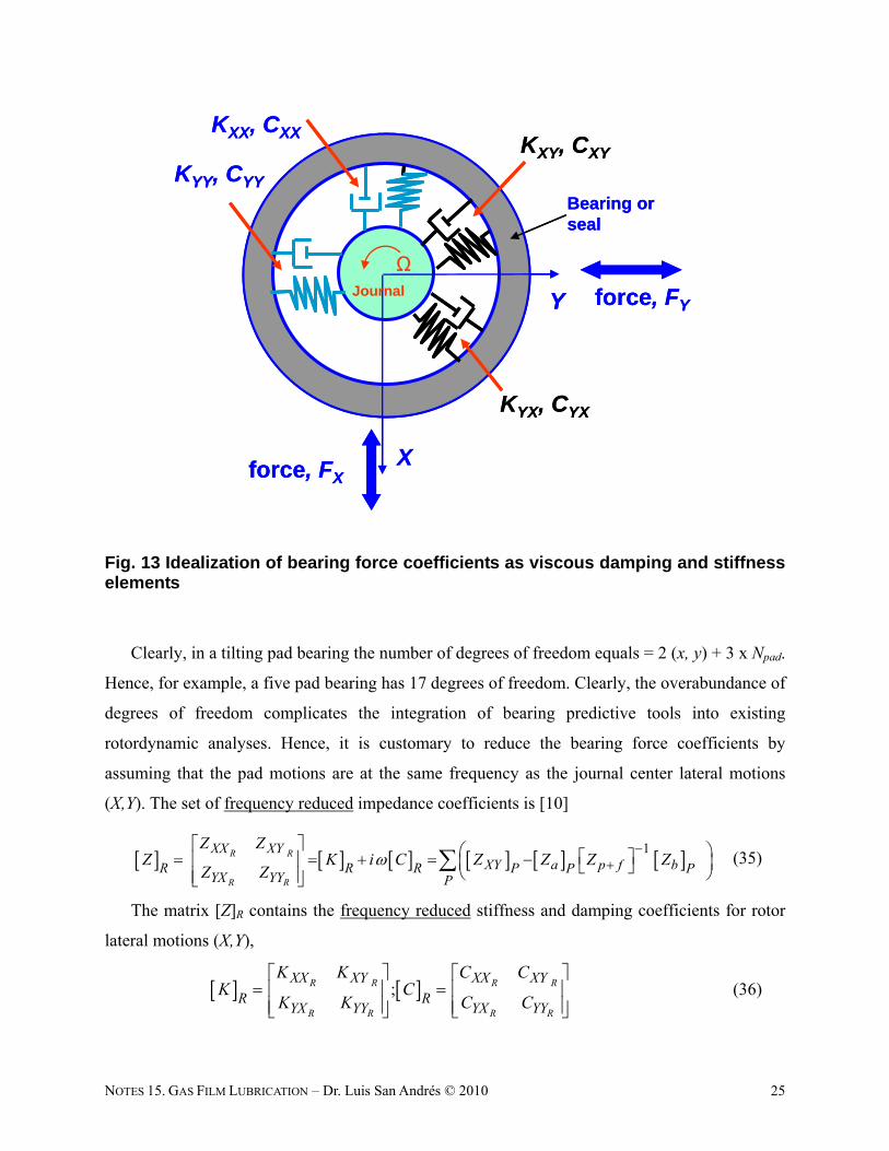
Most analyses consider bearings as two degrees of freedom mechanical elements with lateral
forces reacting to radial displacements (x, y). Bearing rotordynamic force coefficients are, by
definition, changes in reaction forces due to small amplitude motions about an equilibrium
position. The linearized model for a gas bearing is
X XX XY XX XY
Y YX YY YX YY
F K K C Cx x
F K K C Cy y
= F = -K z -Cz (34)
where F=FX, FYT and z=x(t) ,y(t)
T are vectors of lateral reaction forces and displacements,
respectively. Figure 13 shows a schematic idealized representation of the force coefficients as
mechanical spring and viscous dashpot connections between the rotating journal and its bearing.
Recall that gas bearings due to the fluid compressibility will show force coefficients that are
strong functions of the excitation frequency. In tilting pad bearings, the complicated behavior is
further compounded by the pads’ radial and tilting motions.
NOTES 15. GAS FILM LUBRICATION – Dr. Luis San Andrés © 2010 25
X
Y
KYY, CYY
KXY, CXY
force, FY
Bearing or seal
Journal
KYX, CYX
KXX, CXX
Ω
force, FXX
Y
KYY, CYY
KXY, CXY
force, FY
Bearing or seal
Journal
KYX, CYX
KXX, CXX
Ω
force, FX
Fig. 13 Idealization of bearing force coefficients as viscous damping and stiffness elements
Clearly, in a tilting pad bearing the number of degrees of freedom equals = 2 (x, y) + 3 x Npad.
Hence, for example, a five pad bearing has 17 degrees of freedom. Clearly, the overabundance of
degrees of freedom complicates the integration of bearing predictive tools into existing
rotordynamic analyses. Hence, it is customary to reduce the bearing force coefficients by
assuming that the pad motions are at the same frequency as the journal center lateral motions
(X,Y). The set of frequency reduced impedance coefficients is [10]
1R R
R R
XX XYXY a p f bR R R P P P
YX YY P
Z ZZ K i C Z Z Z Z
Z Z
(35)
The matrix [Z]R contains the frequency reduced stiffness and damping coefficients for rotor
lateral motions (X,Y),
;R R R R
R R R R
XX XY XX XY
R RYX YY YX YY
K K C CK C
K K C C
(36)
NOTES 15. GAS FILM LUBRICATION – Dr. Luis San Andrés © 2010 26
In the equation above,
Pxcxb
xaxXY
PYX
YX
YX
YYYYYYX
XXXXYXX
P ZZ
ZZ
ZZZZZ
ZZZZZ
ZZZZZ
ZZZZZ
ZZZZZ
Z
3323
3222
(37a)
and PcSP
SPfP MZCiKZ 2 (37b)
is the composite (pad plus film) impedance matrix at frequency . For prediction of RBS
imbalance responses, synchronous force coefficients are calculated with . For eigenvalue
RBS analysis, i.e. prediction of damped natural frequencies and damping ratios, iterative
methods allow the determination of the coefficients at frequencies coinciding with the RBS
natural frequencies.
As emphasized earlier, gas bearings (rigid surfaces, tilting pads and foil types) have
frequency dependent force coefficients because of the fluid compressibility and the compliance
of the bearing par surfaces. The dependency on frequency cannot be overlooked!
Some considerations on the solution of Reynolds equation for gas films
Most often the numerical solution of Reynolds equations (equilibrium and its variations for
the dynamic first order pressure fields) is performed using algorithms suited for elliptical-type
differential equations. Note also that Reynolds equation for the generation of gas film pressure is
nonlinear due to the density varying with the pressure. In the case of a hydrostatic bearing
carrying a static load, the equation becomes linear, i.e., Eq. (19) reduces to
32 0
24
hp
(38)
This equation can be solved efficiently for (p2) as the independent variable with either central
finite differences or finite element methods.
However, the more general bearing case that includes both hydrodynamic and hydrostatic
effects remains nonlinear. In particular, one must realize that for large rotor speeds
and/or large whirl frequencies , the character of the Reynolds equation
NOTES 15. GAS FILM LUBRICATION – Dr. Luis San Andrés © 2010 27
changes from elliptical to parabolic. Recall, in dimensionless form, that the compressible fluid
film Reynolds equation is
3 3P PP H P H P H P H
z z
(39)
where 2 2
12
6 12and
a a
R R
p c p c
(4)
are the well-known speed and frequency numbers, respectively. At large speed numbers or
frequency numbers 1, 1 , the first order terms on the right hand side dominate the
generation of the hydrodynamic pressure in the gas film region. For low rotational speeds ()
and low frequencies, i.e., , 0 , the expansion 1P P gives the linearized Reynolds
equation
3 312
P P H HH H
z z
(40)
which is elliptical in character and formally identical to the Reynolds equation for an
incompressible fluid. The numerical solution of the linear equation above can be easily
performed using (central) finite differences, for example. More importantly, any predictive
computational tool predicting pressure fields for bearings lubricated with incompressible fluids
(oils) can also be used for gas films operating at low rotational speeds and/or low whirl
frequencies. See Lecture Notes 7 for details on the numerical solution of Eq. (40)
For operation with large speeds, the infinite speed equation for pressure generation
is
0 a
ah
p h p ph
(41)
which12 establishes a limit on the generation of hydrodynamic pressure in a radial bearing.
Consequently, the bearing reaction load will also reach a definite limit. The ultimate load
capacity (wu) of the cylindrical gas bearing is, as , [3]
12 This solution is to be taken with caution since it does not satisfy all the boundary conditions, in particular at the bearing axial edges, i.e.,
2at L
ap p z
NOTES 15. GAS FILM LUBRICATION – Dr. Luis San Andrés © 2010 28
1/222
max1/22
0
1 1 11 cos
2 1 cos 1u
a
Ww d
p L D
(42)
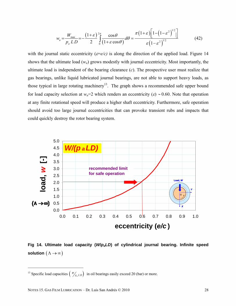
with the journal static eccentricity (=e/c) is along the direction of the applied load. Figure 14
shows that the ultimate load (wu) grows modestly with journal eccentricity. Most importantly, the
ultimate load is independent of the bearing clearance (c). The prospective user must realize that
gas bearings, unlike liquid lubricated journal bearings, are not able to support heavy loads, as
those typical in large rotating machinery13. The graph shows a recommended safe upper bound
for load capacity selection at wu=2 which renders an eccentricity () 0.60. Note that operation
at any finite rotational speed will produce a higher shaft eccentricity. Furthermore, safe operation
should avoid too large journal eccentricities that can provoke transient rubs and impacts that
could quickly destroy the rotor bearing system.
0.0
0.5
1.0
1.5
2.0
2.5
3.0
3.5
4.0
4.5
5.0
0.0 0.1 0.2 0.3 0.4 0.5 0.6 0.7 0.8 0.9 1.0
eccentricity (e/c )
loa
d, w
[-]
W/(p a LD)
recommended limit for safe operation
X
Y
Load, W
X
Y
Load, W
Fig 14. Ultimate load capacity (W/paLD) of cylindrical journal bearing. Infinite speed
solution
13 Specific load capacities a
Wp L D in oil bearings easily exceed 20 (bar) or more.
NOTES 15. GAS FILM LUBRICATION – Dr. Luis San Andrés © 2010 29
Incidentally, for operation with infinite frequency , and for simplicity not
accounting for shear flow effects 0 , the squeeze film pressure is just
0
,a
ah
p h p ph
(43)
Thus, the pressure is in-phase with the film thickness, i.e., solely determined by the
displacements YX e,e and not its time variations, i.e., not a function of the velocity at which the
film thickness changes. These operating conditions thus lead to a stiffening or hardening of the
gas film and absence of squeeze film damping effects. Examples showing this behavior were
introduced for one-dimensional slider bearings.
Importantly enough, high frequency motions of a squeeze gas film can generate a mean
pressure above ambient; and hence the ability to carry a static load (albeit small). See Ref. [2] for
details on this rectification phenomenon.
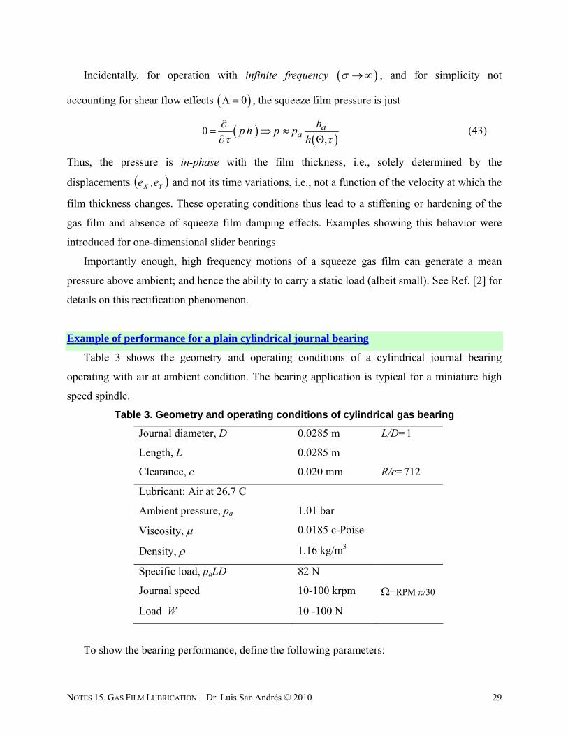
Example of performance for a plain cylindrical journal bearing
Table 3 shows the geometry and operating conditions of a cylindrical journal bearing
operating with air at ambient condition. The bearing application is typical for a miniature high
speed spindle.
Table 3. Geometry and operating conditions of cylindrical gas bearing
Journal diameter, D 0.0285 m L/D=1
Length, L 0.0285 m
Clearance, c 0.020 mm R/c=712
Lubricant: Air at 26.7 C
Ambient pressure, pa 1.01 bar
Viscosity, 0.0185 c-Poise
Density, 1.16 kg/m3
Specific load, paLD 82 N
Journal speed 10-100 krpm RPM /30
Load W 10 -100 N
To show the bearing performance, define the following parameters:
NOTES 15. GAS FILM LUBRICATION – Dr. Luis San Andrés © 2010 30
a
Ww
p L D ,
2N L D R
SW c
, 2
6
a
R L
p c
(44)
which represent the dimensionless load, Sommerfeld number and speed (or compressibility)
number, respectively. Above N is the rotational speed in rev/s. Note that in the design (and
selection) of a gas bearing the Sommerfeld number is (usually) known or serves to size the
bearing clearance14.
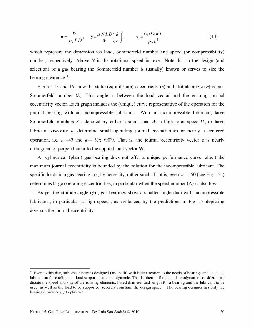
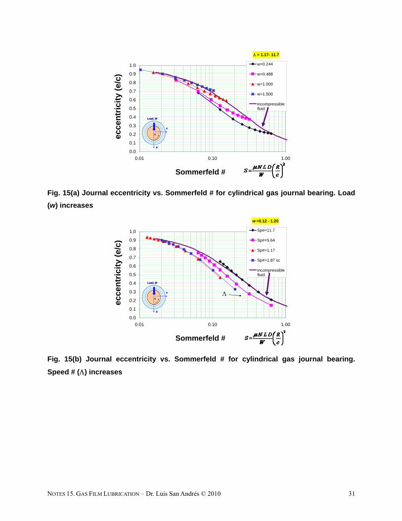
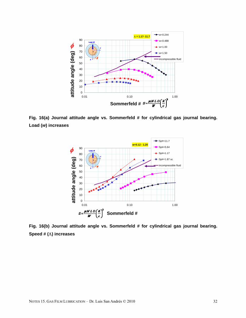
Figures 15 and 16 show the static (equilibrium) eccentricity () and attitude angle () versus
Sommerfeld number (S). This angle is between the load vector and the ensuing journal
eccentricity vector. Each graph includes the (unique) curve representative of the operation for the
journal bearing with an incompressible lubricant. With an incompressible lubricant, large
Sommerfeld numbers S , denoted by either a small load W, a high rotor speed , or large
lubricant viscosity , determine small operating journal eccentricities or nearly a centered
operation, i.e. 0 and ½ (90). That is, the journal eccentricity vector e is nearly
orthogonal or perpendicular to the applied load vector W.
A cylindrical (plain) gas bearing does not offer a unique performance curve; albeit the
maximum journal eccentricity is bounded by the solution for the incompressible lubricant. The
specific loads in a gas bearing are, by necessity, rather small. That is, even w=1.50 (see Fig. 15a)
determines large operating eccentricities, in particular when the speed number () is also low.
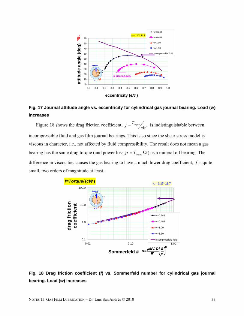
As per the attitude angle ( , gas bearings show a smaller angle than with incompressible
lubricants, in particular at high speeds, as evidenced by the predictions in Fig. 17 depicting
versus the journal eccentricity.
14 Even to this day, turbomachinery is designed (and built) with little attention to the needs of bearings and adequate lubrication for cooling and load support, static and dynamic. That is, thermo fluidic and aerodynamic considerations dictate the speed and size of the rotating elements. Fixed diameter and length for a bearing and the lubricant to be used, as well as the load to be supported, severely constrain the design space. The bearing designer has only the bearing clearance (c) to play with.
NOTES 15. GAS FILM LUBRICATION – Dr. Luis San Andrés © 2010 31
= 1.17- 11.7
0.0
0.1
0.2
0.3
0.4
0.5
0.6
0.7
0.8
0.9
1.0
0.01 0.10 1.00
Sommerfeld #
ecce
ntr
icit
y (e
/c)
w=0.244
w=0.488
w=1.000
w=1.500
incompressiblefluid
X
Y
Load, W
X
Y
Load, W
Fig. 15(a) Journal eccentricity vs. Sommerfeld # for cylindrical gas journal bearing. Load
(w) increases
w =0.12 - 1.20
0.0
0.1
0.2
0.3
0.4
0.5
0.6
0.7
0.8
0.9
1.0
0.01 0.10 1.00
Sommerfeld #
ecce
ntr
icit
y (e
/c)
Sp#=11.7
Sp#=5.64
Sp#=1.17
Sp#=1.87 sc
incompressiblefluid
X
Y
Load, W
X
Y
Load, W
Fig. 15(b) Journal eccentricity vs. Sommerfeld # for cylindrical gas journal bearing.
Speed # () increases
NOTES 15. GAS FILM LUBRICATION – Dr. Luis San Andrés © 2010 32
= 1.17- 11.7
0
10
20
30
40
50
60
70
80
90
0.01 0.10 1.00
Sommerfeld #
atti
tud
e an
gle
(d
eg)
w=0.244
w=0.488
w=1.00
w=1.50
incompressible fluid
X
Y
Load, W
X
Y
Load, W
Fig. 16(a) Journal attitude angle vs. Sommerfeld # for cylindrical gas journal bearing.
Load (w) increases
w=0.12 - 1.20
0
10
20
30
40
50
60
70
80
90
0.01 0.10 1.00
Sommerfeld #
atti
tud
e an
gle
(d
eg)
Sp#=11.7
Sp#=5.64
Sp#=1.17
Sp#=1.87 sc
incompressible fluid
X
Y
Load, W
X
Y
Load, W
Fig. 16(b) Journal attitude angle vs. Sommerfeld # for cylindrical gas journal bearing.
Speed # () increases
NOTES 15. GAS FILM LUBRICATION – Dr. Luis San Andrés © 2010 33
= 1.17- 11.7
0
10
20
30
40
50
60
70
80
90
0.0 0.1 0.2 0.3 0.4 0.5 0.6 0.7 0.8 0.9 1.0
eccentricity (e/c )
att
itu
de
ang
le (
de
g)
w=0.244
w=0.488
w=1.00
w=1.50
incompressible fluid
X
Y
Load, W
X
Y
Load, W
increases
Fig. 17 Journal attitude angle vs. eccentricity for cylindrical gas journal bearing. Load (w)
increases
Figure 18 shows the drag friction coefficient, orqueTf cW , is indistinguishable between
incompressible fluid and gas film journal bearings. This is so since the shear stress model is
viscous in character, i.e., not affected by fluid compressibility. The result does not mean a gas
bearing has the same drag torque (and power loss orqueT ) as a mineral oil bearing. The
difference in viscosities causes the gas bearing to have a much lower drag coefficient; f is quite
small, two orders of magnitude at least.
f=Torque/ (cW )
0.1
1.0
10.0
100.0
0.01 0.10 1.00
Sommerfeld #
dra
g f
rict
ion
co
effi
cien
t
w=0.244
w=0.488
w=1.00
w=1.50
incompressible fluid
X
Y
Load, W
X
Y
Load, W
= 1.17- 11.7
Fig. 18 Drag friction coefficient (f) vs. Sommerfeld number for cylindrical gas journal
bearing. Load (w) increases
NOTES 15. GAS FILM LUBRICATION – Dr. Luis San Andrés © 2010 34
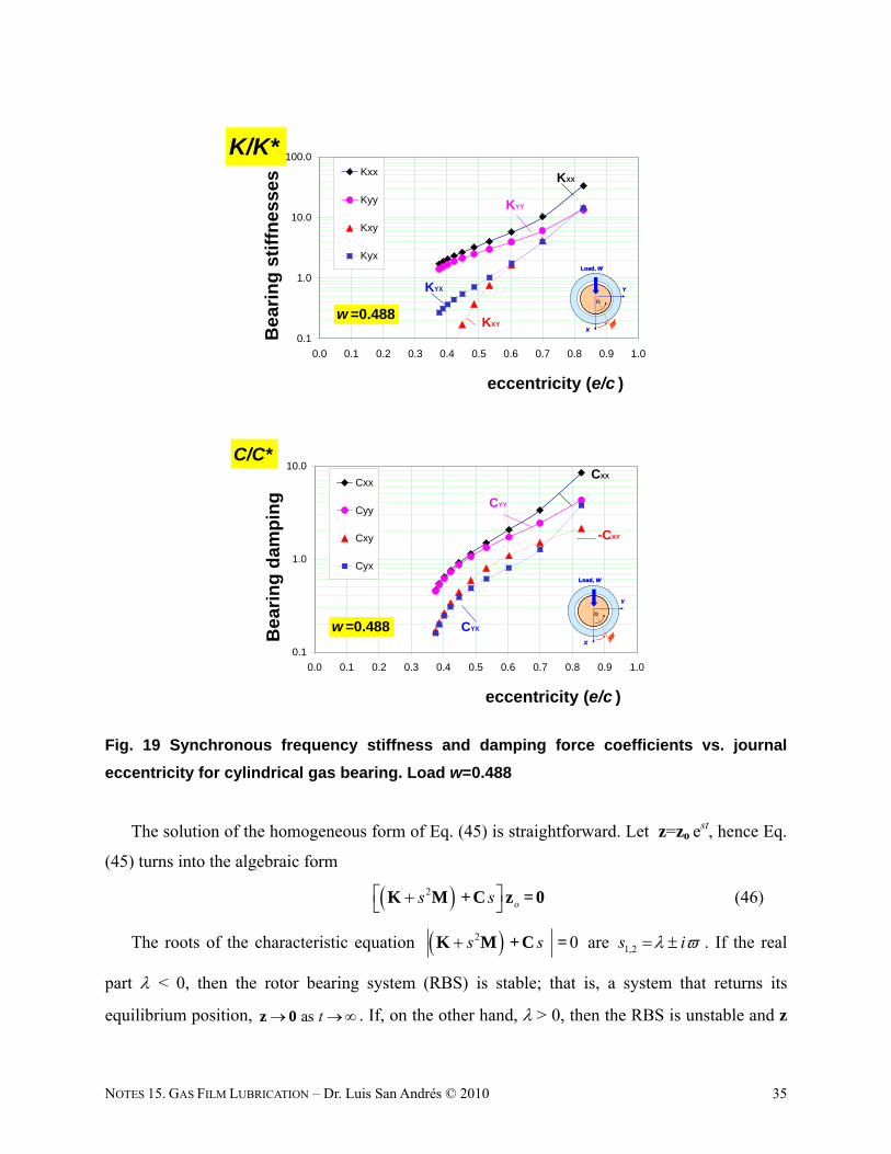
Bearing force coefficients and dynamic stability
Figure 19 depicts the bearing stiffness and damping force coefficients evaluated at a
frequency coinciding with the journal rotational speed (). In the example, the dimensionless
load w=0.488 while the journal speed increases from 10 krpm to 100 krpm. Hence, the bearing
Speed number 1.17 to 11.7, and the Sommerfeld number S=0.032 to 0.318. The
dimensionless force coefficients are 3
***
, ; where4
D LCKK C CCC c
. See Fig.
15(a) for the relation between the journal eccentricity and the Sommerfeld number. Note that the
direct stiffnesses (KXX, KYY) and damping (CXX, CYY) coefficients increase with the journal
eccentricity (). At low eccentricities 0 or high speeds , i.e., 1S , then KXY=-
KYX and CXY=-CYX.
The stability of the rotor-bearing system is of interest. In general, this is an elaborate
procedure that requires the integration of the fluid film bearing reaction forces into a
rotordynamics model. Simple analyses consider a point mass (M) rigid rotor supported on a gas
bearing. The (linearized) equations of motion of the system about an equilibrium conditions
(W=F) are
e
e
XXX XY XX XY
YX YY YX YY Y
e
FK K C Cx x xM
K K C Cy y y F
M z + K z +Cz = F
(45)
where z=x(t) ,y(t)T is the vector of dynamic displacements of the journal center. Above,
Fe=FX,FYT is the external dynamic force vector acting on the system, for example due to mass
imbalance. The stability of the system considers the homogeneous form of Eq. (45) and assumes
an initial state i iz , z away from the equilibrium condition (x=y=0).
NOTES 15. GAS FILM LUBRICATION – Dr. Luis San Andrés © 2010 35
K/K*
0.1
1.0
10.0
100.0
0.0 0.1 0.2 0.3 0.4 0.5 0.6 0.7 0.8 0.9 1.0
eccentricity (e/c )
Bea
rin
g s
tiff
nes
ses Kxx
Kyy
Kxy
Kyx
w =0.488
X
Y
Load, W
X
Y
Load, W
KXX
KYY
KXY
KYX
C/C*
0.1
1.0
10.0
0.0 0.1 0.2 0.3 0.4 0.5 0.6 0.7 0.8 0.9 1.0
eccentricity (e/c )
Bea
rin
g d
amp
ing
Cxx
Cyy
Cxy
Cyx
w =0.488
X
Y
Load, W
X
Y
Load, W
CXX
CYY
-CXY
CYX
Fig. 19 Synchronous frequency stiffness and damping force coefficients vs. journal
eccentricity for cylindrical gas bearing. Load w=0.488
The solution of the homogeneous form of Eq. (45) is straightforward. Let z=zo est, hence Eq.
(45) turns into the algebraic form
2os s K M +C z = 0 (46)
The roots of the characteristic equation 2 0s sK M +C = are 1,2s i . If the real
part < 0, then the rotor bearing system (RBS) is stable; that is, a system that returns its
equilibrium position, as t z 0 . If, on the other hand, > 0, then the RBS is unstable and z

NOTES 15. GAS FILM LUBRICATION – Dr. Luis San Andrés © 2010 36
grows without bound15. At the threshold of instability, when = 0, the system will perform self-
excited motions with whirl frequency i.e. z=zo et. Hence, Eq. (46) becomes
2 whereo i Z M z = 0 Z K C (47)
Solution of Eq. (47) is straightforward for incompressible fluid, rigid surface, journal
bearings since their force coefficients are frequency independent. The analysis leads to the
estimation of the system critical mass (MC) and the whirl frequency ratio (WFR) [25]
2 XX YY YY XX YX XY XY YXC S eq
XX YY
K C K C C K C KM K
C C
22 eq XX eq YY XY YXs
XX YY XY YX
K K K K K KWFR
C C C C
(48)
On the other hand, gas bearings have frequency dependent force coefficients, K() and C().
As an example, for the particular operating conditions noted, Fig. 20 depicts the dimensionless
stiffness (Kij)ij=X,Y and damping (Cij)ij=X,Y coefficients versus frequency ratio (where is
the rotational speed; denotes whirl frequency excitation synchronous with the rotational
speed. Note that the direct stiffnesses increase with whirl frequency, a typical hardening effect
due to fluid compressibility. On the other hand, the damping coefficients at high frequencies are
zero, 0asijC , also due to fluid compressibility. An iterative method is required to solve
for the characteristic Eq. (47), 2 0 Z M = . Lund [24] restated Eq. (47) as
2 Z = M ,
and hence the instability threshold occurs at frequency s where the imaginary part of the
complex impedance Ze is zero while its real part must be greater than zero. The equivalent
impedance is
( )
221
4
1
2e XX YY XX YY XY YXZ Z Z Z Z Z Z
(49)
Im 0 and Re 0s s
e eZ Z
(50)
The first statement above implies the effective damping is nil. For the data shown in Fig. 20,
the RBS critical mass is just Mc=0.968 kg and the WFR=0.48. That is, for operation with journal
15 It is a common misconception that the “no bound” statement implies system destruction. In actuality, the journal will whirl with a large amplitude whirl orbit bounded by the bearing clearance. As the motion amplitude grows, the bearing nonlinearity determines the size of the limit cycle. Of course, sustained operating under this condition is not recommended.
NOTES 15. GAS FILM LUBRICATION – Dr. Luis San Andrés © 2010 37
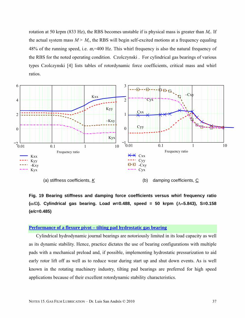
rotation at 50 krpm (833 Hz), the RBS becomes unstable if is physical mass is greater than Mc. If
the actual system mass M > Mc, the RBS will begin self-excited motions at a frequency equaling
48% of the running speed, i.e. s=400 Hz. This whirl frequency is also the natural frequency of
the RBS for the noted operating condition. Czolczynski . For cylindrical gas bearings of various
types Czolczynski [4] lists tables of rotordynamic force coefficients, critical mass and whirl
ratios.
0.01 0.1 1 102
0
2
4
6
KxxKyy-KxyKyx
Frequency ratio
Kxx
Kyy
Kxy
Kyx
0.01 0.1 1 101
0
1
2
3
CxxCyy-CxyCyx
Frequency ratio
CxyCyx
Cxx
Cyy
(a) stiffness coefficients, K (b) damping coefficients, C
Fig. 19 Bearing stiffness and damping force coefficients versus whirl frequency ratio
(). Cylindrical gas bearing. Load w=0.488, speed = 50 krpm (5.843), S=0.158
(e/c=0.485)
Performance of a flexure pivot – tilting pad hydrostatic gas bearing
Cylindrical hydrodynamic journal bearings are notoriously limited in its load capacity as well
as its dynamic stability. Hence, practice dictates the use of bearing configurations with multiple
pads with a mechanical preload and, if possible, implementing hydrostatic pressurization to aid
early rotor lift off as well as to reduce wear during start up and shut down events. As is well
known in the rotating machinery industry, tilting pad bearings are preferred for high speed
applications because of their excellent rotordynamic stability characteristics.
NOTES 15. GAS FILM LUBRICATION – Dr. Luis San Andrés © 2010 38
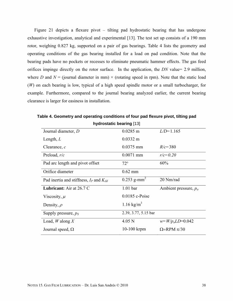
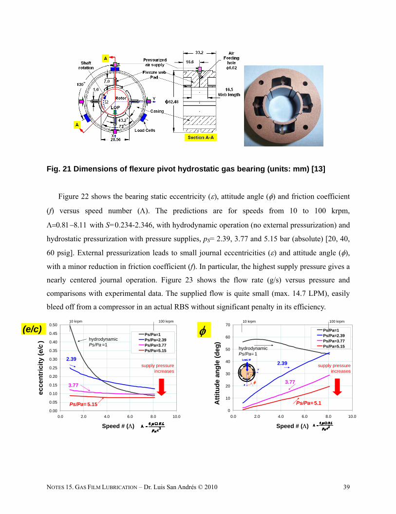
Figure 21 depicts a flexure pivot – tilting pad hydrostatic bearing that has undergone
exhaustive investigation, analytical and experimental [13]. The test set up consists of a 190 mm
rotor, weighing 0.827 kg, supported on a pair of gas bearings. Table 4 lists the geometry and
operating conditions of the gas bearing installed for a load on pad condition. Note that the
bearing pads have no pockets or recesses to eliminate pneumatic hammer effects. The gas feed
orifices impinge directly on the rotor surface. In the application, the DN value= 2.9 million,
where D and N = (journal diameter in mm) × (rotating speed in rpm). Note that the static load
(W) on each bearing is low, typical of a high speed spindle motor or a small turbocharger, for
example. Furthermore, compared to the journal bearing analyzed earlier, the current bearing
clearance is larger for easiness in installation.
Table 4. Geometry and operating conditions of four pad flexure pivot, tilting pad
hydrostatic bearing [13]
Journal diameter, D 0.0285 m L/D=1.165
Length, L 0.0332 m
Clearance, c 0.0375 mm R/c=380
Preload, r/c 0.0071 mm r/c=0.20
Pad arc length and pivot offset 72 60%
Orifice diameter 0.62 mm
Pad inertia and stiffness, IP and K 0.253 g-mm2 20 Nm/rad
Lubricant: Air at 26.7 C 1.01 bar Ambient pressure, pa
Viscosity, 0.0185 c-Poise
Density, 1.16 kg/m3
Supply pressure, pS 2.39, 3.77, 5.15 bar
Load, W along X 4.05 N w=W/paLD=0.042
Journal speed, 10-100 krpm RPM /30
NOTES 15. GAS FILM LUBRICATION – Dr. Luis San Andrés © 2010 39
Fig. 21 Dimensions of flexure pivot hydrostatic gas bearing (units: mm) [13]
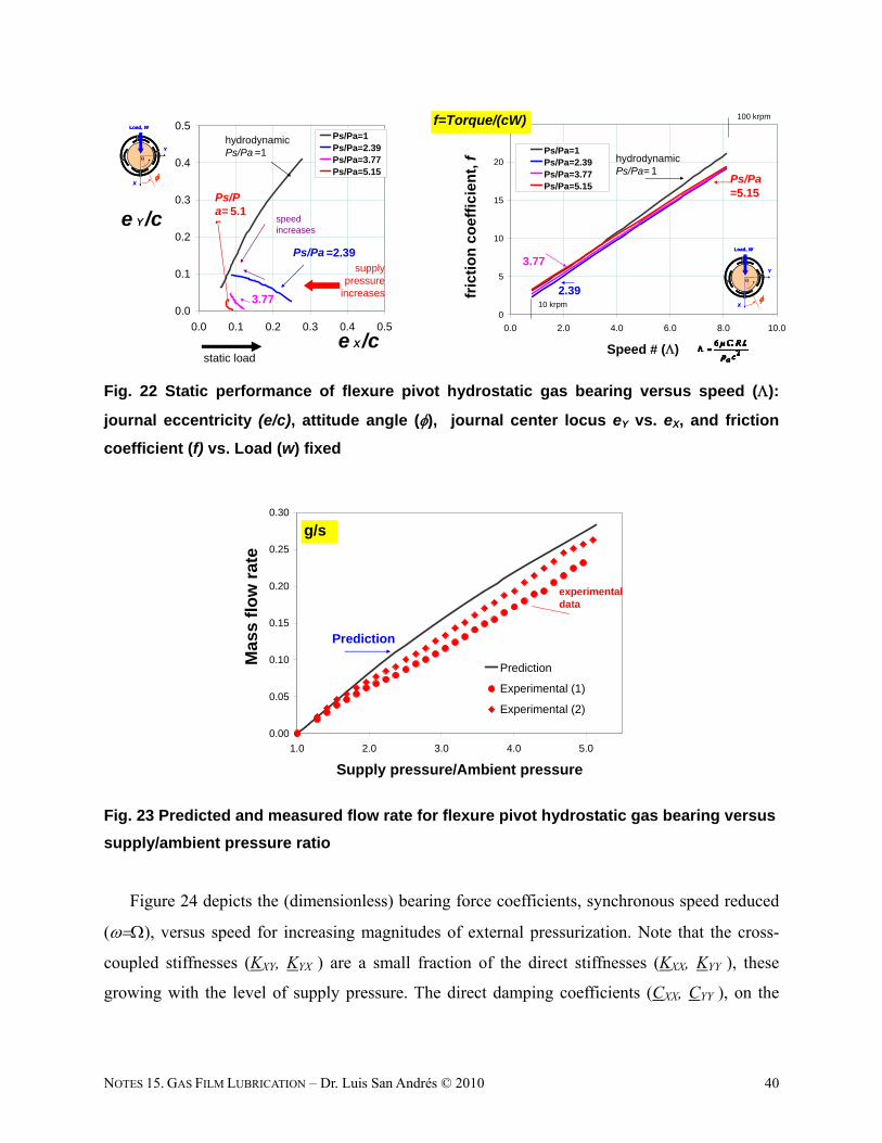
Figure 22 shows the bearing static eccentricity (), attitude angle () and friction coefficient
(f) versus speed number (). The predictions are for speeds from 10 to 100 krpm,
with S=0.234-2.346, with hydrodynamic operation (no external pressurization) and
hydrostatic pressurization with pressure supplies, pS= 2.39, 3.77 and 5.15 bar (absolute) [20, 40,
60 psig]. External pressurization leads to small journal eccentricities () and attitude angle (),
with a minor reduction in friction coefficient (f). In particular, the highest supply pressure gives a
nearly centered journal operation. Figure 23 shows the flow rate (g/s) versus pressure and
comparisons with experimental data. The supplied flow is quite small (max. 14.7 LPM), easily
bleed off from a compressor in an actual RBS without significant penalty in its efficiency.
0.00
0.05
0.10
0.15
0.20
0.25
0.30
0.35
0.40
0.45
0.50
0.0 2.0 4.0 6.0 8.0 10.0
Speed # ()
ecce
ntr
icit
y (e
/c)
Ps/Pa=1Ps/Pa=2.39 Ps/Pa=3.77Ps/Pa=5.15
(e/c)
Ps/Pa= 5.15
3.77
2.39
hydrodynamicPs/Pa =1
supply pressureincreases
10 krpm 100 krpm
0
10
20
30
40
50
60
70
0.0 2.0 4.0 6.0 8.0 10.0
Speed # ()
Att
itu
de
ang
le (
deg
)
Ps/Pa=1Ps/Pa=2.39Ps/Pa=3.77Ps/Pa=5.15
Ps/Pa= 5.1
3.77
2.39
hydrodynamicPs/Pa= 1
supply pressure increases
10 krpm 100 krpm
X
Y
Load, W
X
Y
Load, W
NOTES 15. GAS FILM LUBRICATION – Dr. Luis San Andrés © 2010 40
0.0
0.1
0.2
0.3
0.4
0.5
0.0 0.1 0.2 0.3 0.4 0.5
e X/c
e Y/c
Ps/Pa=1Ps/Pa=2.39 Ps/Pa=3.77Ps/Pa=5.15
Ps/Pa= 5.15
3.77
Ps/Pa =2.39
hydrodynamicPs/Pa =1
supply pressure
increases
static load
speed increases
X
Y
Load, W
X
Y
Load, W
0
5
10
15
20
25
0.0 2.0 4.0 6.0 8.0 10.0
Speed # ()
fric
tio
n c
oef
fici
ent,
f
Ps/Pa=1Ps/Pa=2.39 Ps/Pa=3.77Ps/Pa=5.15
f=Torque/(cW)
Ps/Pa=5.15
3.77
2.39
hydrodynamicPs/Pa= 1
10 krpm
100 krpm
X
Y
Load, W
X
Y
Load, W
Fig. 22 Static performance of flexure pivot hydrostatic gas bearing versus speed ():
journal eccentricity (e/c), attitude angle (), journal center locus eY vs. eX, and friction
coefficient (f) vs. Load (w) fixed
0.00
0.05
0.10
0.15
0.20
0.25
0.30
1.0 2.0 3.0 4.0 5.0
Supply pressure/Ambient pressure
Ma
ss f
low
rat
e
Prediction
Experimental (1)
Experimental (2)
g/s
Prediction
experimentaldata
Fig. 23 Predicted and measured flow rate for flexure pivot hydrostatic gas bearing versus
supply/ambient pressure ratio
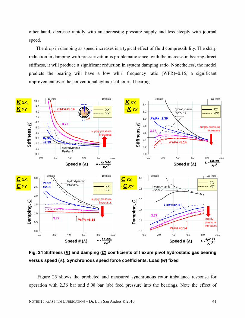
Figure 24 depicts the (dimensionless) bearing force coefficients, synchronous speed reduced
(), versus speed for increasing magnitudes of external pressurization. Note that the cross-
coupled stiffnesses (KXY, KYX ) are a small fraction of the direct stiffnesses (KXX, KYY ), these
growing with the level of supply pressure. The direct damping coefficients (CXX, CYY ), on the
NOTES 15. GAS FILM LUBRICATION – Dr. Luis San Andrés © 2010 41
other hand, decrease rapidly with an increasing pressure supply and less steeply with journal
speed.
The drop in damping as speed increases is a typical effect of fluid compressibility. The sharp
reduction in damping with pressurization is problematic since, with the increase in bearing direct
stiffness, it will produce a significant reduction in system damping ratio. Nonetheless, the model
predicts the bearing will have a low whirl frequency ratio (WFR)~0.15, a significant
improvement over the conventional cylindrical journal bearing.
0.0
1.0
2.0
3.0
4.0
5.0
6.0
7.0
8.0
9.0
10.0
0.0 2.0 4.0 6.0 8.0 10.0
Speed # ()
Sti
ffn
ess,
K
K XX,
K YY Ps/Pa =5.14
3.77
hydrodynamicPs/Pa =1
supply pressureincreases
10 krpm 100 krpm
Ps/Pa=2.39
XXYY
X
Y
Load, W
X
Y
Load, W
0.0
0.2
0.4
0.6
0.8
1.0
1.2
1.4
0.0 2.0 4.0 6.0 8.0 10.0
Speed # ()
Sti
ffn
ess,
K
K XY,
- K YX
Ps/Pa =5.14
3.77
Ps/Pa =2.39
supply pressure increases
10 krpm 100 krpm
XY-YX
hydrodynamicPs/Pa =1
0.0
0.5
1.0
1.5
2.0
2.5
3.0
0.0 2.0 4.0 6.0 8.0 10.0
Speed # ()
Dam
pin
g,
C
C XX,
C YY
Ps/Pa =5.143.77
Ps/Pa= 2.39
supply pressureincreases
10 krpm 100 krpm
hydrodynamicPs/Pa =1 XX
YY
0.0
0.2
0.4
0.6
0.8
1.0
0.0 2.0 4.0 6.0 8.0 10.0
Speed # ()
Dam
pin
g,
C
C YX,
- C XY
Ps/Pa =5.14
3.77
Ps/Pa =2.39
hydrodynamicPs/Pa =1
supply pressure increases
10 krpm 100 krpm
YX-XY
Fig. 24 Stiffness (K) and damping (C) coefficients of flexure pivot hydrostatic gas bearing
versus speed (). Synchronous speed force coefficients. Load (w) fixed
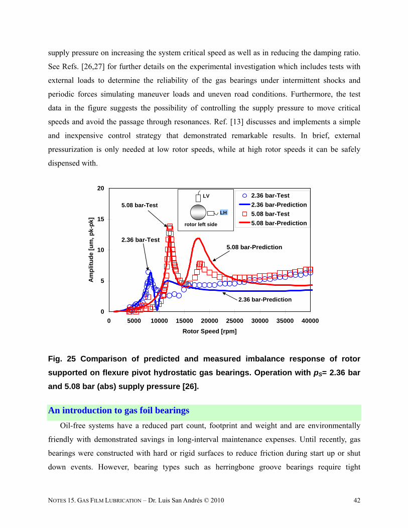
Figure 25 shows the predicted and measured synchronous rotor imbalance response for
operation with 2.36 bar and 5.08 bar (ab) feed pressure into the bearings. Note the effect of
NOTES 15. GAS FILM LUBRICATION – Dr. Luis San Andrés © 2010 42
supply pressure on increasing the system critical speed as well as in reducing the damping ratio.
See Refs. [26,27] for further details on the experimental investigation which includes tests with
external loads to determine the reliability of the gas bearings under intermittent shocks and
periodic forces simulating maneuver loads and uneven road conditions. Furthermore, the test
data in the figure suggests the possibility of controlling the supply pressure to move critical
speeds and avoid the passage through resonances. Ref. [13] discusses and implements a simple
and inexpensive control strategy that demonstrated remarkable results. In brief, external
pressurization is only needed at low rotor speeds, while at high rotor speeds it can be safely
dispensed with.
0
5
10
15
20
0 5000 10000 15000 20000 25000 30000 35000 40000
Rotor Speed [rpm]
Am
plit
ud
e [
um
, p
k-p
k]
2.36 bar-Test
2.36 bar-Prediction
5.08 bar-Test
5.08 bar-Prediction
5.08 bar-Test
2.36 bar-Prediction
LH
LV
rotor left side
2.36 bar-Test5.08 bar-Prediction
Fig. 25 Comparison of predicted and measured imbalance response of rotor
supported on flexure pivot hydrostatic gas bearings. Operation with pS= 2.36 bar
and 5.08 bar (abs) supply pressure [26].
An introduction to gas foil bearings
Oil-free systems have a reduced part count, footprint and weight and are environmentally
friendly with demonstrated savings in long-interval maintenance expenses. Until recently, gas
bearings were constructed with hard or rigid surfaces to reduce friction during start up or shut
down events. However, bearing types such as herringbone groove bearings require tight
NOTES 15. GAS FILM LUBRICATION – Dr. Luis San Andrés © 2010 43
clearances (film thicknesses), and with their hard surfaces offer few advantages for use in high
speed MTM.
Gas foil bearings (GFBs) have emerged as a most efficient alternative for load support in
high speed machinery. These bearings are compliant surface hydrodynamic bearings using
ambient air as the working fluid media. Recall Fig. 1 showing two typical GFB configurations,
one is a multiple overleaf bearing and the other is a corrugated bump bearing. Both bearing types
are used in commercial rotating machinery, yet the open literature presents more details on
bump-GFBs, along with measurements and analyses. The corrugated bump foil bearing is
constructed from one or more layers of corrugated thin metal strips and a top foil. In operation, a
minute gas film wedge develops between the spinning rotor and top foil. The bump-strip layers
are an elastic support with engineered stiffness and damping characteristics [5,18].
GFBs offer distinct advantages over rolling elements bearings including no DN16 value limit,
reliable high temperature operation, and large tolerance to debris and rotor motions, including
temporary rubbing and misalignment, Current commercial applications include auxiliary power
units, cryogenic turbo expanders and micro gas turbines. Envisioned or under development
applications include automotive turbocharger and aircraft gas turbine engines for regional jets
and helicopter rotorcraft systems [5]. Alas, GFBs have demerits of excessive power losses and
wear of protective coatings during rotor startup and shutdown events. In addition, expensive
developmental costs and, until recently, inadequate predictive tools limited the widespread
deployment of GFBs into mid size gas turbines. In particular, at high temperature conditions,
reliable operation of GFB supported rotor systems depends on adequate engineered thermal
management and proven solid lubricants (coatings).
Successful implementation of GFBs in commercial rotating machinery involves a two-tier
effort; that of developing bearing structural components and solid lubricant coatings to increase
the bearing load capacity while reducing friction, and that of developing accurate performance
prediction models anchored to dependable (non commercial) test data. Chen et al. [18] and
DellaCorte et al. [5,28] publicize details on the design and construction of first generation foil
bearings, radial and thrust types, aiming towards their wide adoption in industry.
16 DN, the product of journal diameter (mm) times rotational speed [RPM], is a limiting factor for operation of rolling element bearings (DN= 2 Million in specialized bearings with ceramic balls, for example)
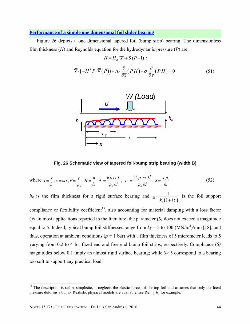
NOTES 15. GAS FILM LUBRICATION – Dr. Luis San Andrés © 2010 44
Performance of a simple one dimensional foil slider bearing
Figure 26 depicts a one dimensional tapered foil (bump strip) bearing. The dimensionless
film thickness (H) and Reynolds equation for the hydrodynamic pressure (P) are:
( ) ( 1)RH H x S P ;
3 0H P P P H P Hx
(51)
LTL
hiho
W (Load)
U
x
LTL
hiho
W (Load)
U
x
Fig. 26 Schematic view of tapered foil-bump strip bearing (width B)
where *
, , ,a
x p hx t P H
L p h
2
2 2* * *
6 12, , a
a a
s pU L LS
p h p h h
(52)
hR is the film thickness for a rigid surface bearing and
1
1b
sk i
is the foil support
compliance or flexibility coefficient17, also accounting for material damping with a loss factor
(). In most applications reported in the literature, the parameter (S) does not exceed a magnitude
equal to 5. Indeed, typical bump foil stiffnesses range from kB = 5 to 100 (MN/m2)/mm [18], and
thus, operation at ambient conditions (pa= 1 bar) with a film thickness of 5 micrometer leads to S
varying from 0.2 to 4 for fixed end and free end bump-foil strips, respectively. Compliance (S)
magnitudes below 0.1 imply an almost rigid surface bearing; while S> 5 correspond to a bearing
too soft to support any practical load.
17 The description is rather simplistic, it neglects the elastic forces of the top foil and assumes that only the local pressure deforms a bump. Realistic physical models are available, see Ref. [16] for example.
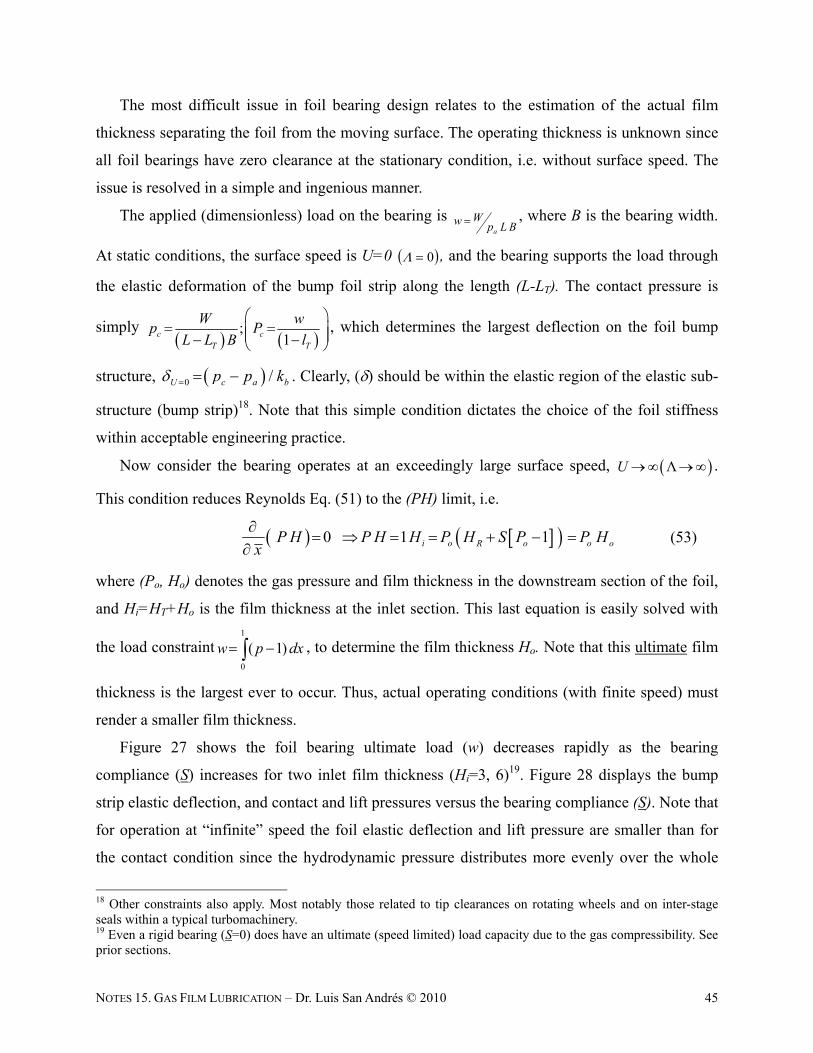
NOTES 15. GAS FILM LUBRICATION – Dr. Luis San Andrés © 2010 45
The most difficult issue in foil bearing design relates to the estimation of the actual film
thickness separating the foil from the moving surface. The operating thickness is unknown since
all foil bearings have zero clearance at the stationary condition, i.e. without surface speed. The
issue is resolved in a simple and ingenious manner.
The applied (dimensionless) load on the bearing is a
Ww p L B , where B is the bearing width.
At static conditions, the surface speed is U=0 0 , and the bearing supports the load through
the elastic deformation of the bump foil strip along the length (L-LT). The contact pressure is
simply
;1c c
T T
W wp P
L L B l
, which determines the largest deflection on the foil bump
structure, 0 /U c a bp p k . Clearly, () should be within the elastic region of the elastic sub-
structure (bump strip)18. Note that this simple condition dictates the choice of the foil stiffness
within acceptable engineering practice.
Now consider the bearing operates at an exceedingly large surface speed, ΛU .
This condition reduces Reynolds Eq. (51) to the (PH) limit, i.e.
0 1 1i o R o o oP H P H H P H S P P Hx
(53)
where (Po, Ho) denotes the gas pressure and film thickness in the downstream section of the foil,
and Hi=HT+Ho is the film thickness at the inlet section. This last equation is easily solved with
the load constraint1
0
( 1)w p dx , to determine the film thickness Ho. Note that this ultimate film
thickness is the largest ever to occur. Thus, actual operating conditions (with finite speed) must
render a smaller film thickness.
Figure 27 shows the foil bearing ultimate load (w) decreases rapidly as the bearing
compliance (S) increases for two inlet film thickness (Hi=3, 6)19. Figure 28 displays the bump
strip elastic deflection, and contact and lift pressures versus the bearing compliance (S). Note that
for operation at “infinite” speed the foil elastic deflection and lift pressure are smaller than for
the contact condition since the hydrodynamic pressure distributes more evenly over the whole
18 Other constraints also apply. Most notably those related to tip clearances on rotating wheels and on inter-stage seals within a typical turbomachinery. 19 Even a rigid bearing (S=0) does have an ultimate (speed limited) load capacity due to the gas compressibility. See prior sections.
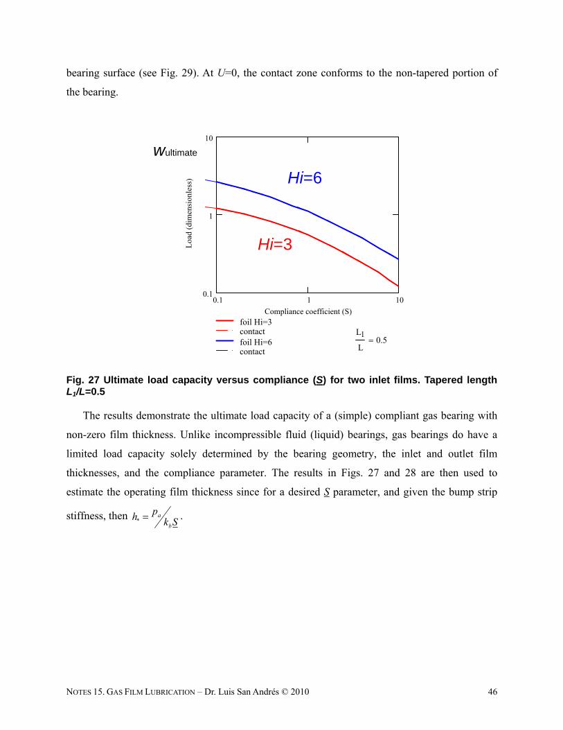
NOTES 15. GAS FILM LUBRICATION – Dr. Luis San Andrés © 2010 46
bearing surface (see Fig. 29). At U=0, the contact zone conforms to the non-tapered portion of
the bearing.
0.1 1 100.1
1
10
foil Hi=3contactfoil Hi=6contact
Compliance coefficient (S)
Loa
d (d
imen
sion
less
)
L1
L0.5
wultimate
Hi=6
Hi=3
Fig. 27 Ultimate load capacity versus compliance (S) for two inlet films. Tapered length L1/L=0.5
The results demonstrate the ultimate load capacity of a (simple) compliant gas bearing with
non-zero film thickness. Unlike incompressible fluid (liquid) bearings, gas bearings do have a
limited load capacity solely determined by the bearing geometry, the inlet and outlet film
thicknesses, and the compliance parameter. The results in Figs. 27 and 28 are then used to
estimate the operating film thickness since for a desired S parameter, and given the bump strip
stiffness, then *a
b
ph k S .
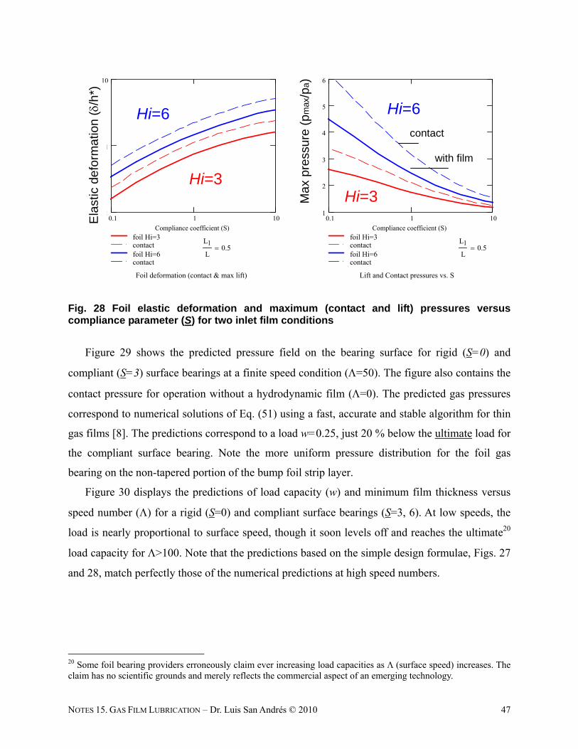
NOTES 15. GAS FILM LUBRICATION – Dr. Luis San Andrés © 2010 47
0.1 1 100.1
1
10
foil Hi=3contact foil Hi=6contact
Foil deformation (contact & max lift)
Compliance coefficient (S)
elas
tic
defo
rmat
ion
(d/h
*)
0.1 1 101
2
3
4
5
6
foil Hi=3contact foil Hi=6contact
Lift and Contact pressures vs. S
Compliance coefficient (S)
Max
pre
ssur
e/P
amb
L1
L0.5
L1
L0.5
Ma
x pr
essu
re (
pm
ax/p
a)
Ela
stic
def
orm
atio
n (
/h*)
Hi=6
Hi=3
Hi=6
Hi=3
contact
with film
Fig. 28 Foil elastic deformation and maximum (contact and lift) pressures versus compliance parameter (S) for two inlet film conditions
Figure 29 shows the predicted pressure field on the bearing surface for rigid (S=0) and
compliant (S=3) surface bearings at a finite speed condition (=50). The figure also contains the
contact pressure for operation without a hydrodynamic film (=0). The predicted gas pressures
correspond to numerical solutions of Eq. (51) using a fast, accurate and stable algorithm for thin
gas films [8]. The predictions correspond to a load w=0.25, just 20 % below the ultimate load for
the compliant surface bearing. Note the more uniform pressure distribution for the foil gas
bearing on the non-tapered portion of the bump foil strip layer.
Figure 30 displays the predictions of load capacity (w) and minimum film thickness versus
speed number () for a rigid (S=0) and compliant surface bearings (S=3, 6). At low speeds, the
load is nearly proportional to surface speed, though it soon levels off and reaches the ultimate20
load capacity for >100. Note that the predictions based on the simple design formulae, Figs. 27
and 28, match perfectly those of the numerical predictions at high speed numbers.
20 Some foil bearing providers erroneously claim ever increasing load capacities as (surface speed) increases. The claim has no scientific grounds and merely reflects the commercial aspect of an emerging technology.
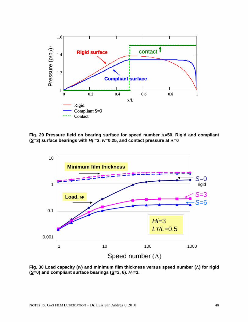
NOTES 15. GAS FILM LUBRICATION – Dr. Luis San Andrés © 2010 48
0 0.2 0.4 0.6 0.8 11
1.2
1.4
1.6
RigidCompliant S=3Contact
x/L
Dim
pre
ssur
e (P
/Pa)
W 0.25
hi 3 HT 2
50
Pre
ssur
e (p
/pa) contactRigid surface
Compliant surface
0 0.2 0.4 0.6 0.8 11
1.2
1.4
1.6
RigidCompliant S=3Contact
x/L
Dim
pre
ssur
e (P
/Pa)
W 0.25
hi 3 HT 2
50
Pre
ssur
e (p
/pa) contactRigid surface
Compliant surface
Fig. 29 Pressure field on bearing surface for speed number =50. Rigid and compliant (S=3) surface bearings with Hi =3, w=0.25, and contact pressure at =0
0.01
0.1
1
10
1 10 100 1000
Speed number
Dim
ensi
on
less
Lo
ad [
-] a
nd
film
th
ickn
ess
[h]
W S=0
W S=3
W S=6
Hmin, S=3
Hmin, S=6
Speed number
1 10 100 1000
10
1
0.1
0.001
S=0
S=3S=6
Minimum film thickness
Load, w
Hi=3 LT/L=0.5
rigid
Fig. 30 Load capacity (w) and minimum film thickness versus speed number () for rigid (S=0) and compliant surface bearings (S=3, 6). Hi =3.
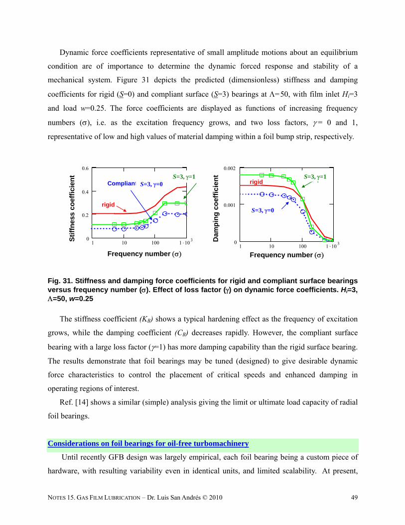
NOTES 15. GAS FILM LUBRICATION – Dr. Luis San Andrés © 2010 49
Dynamic force coefficients representative of small amplitude motions about an equilibrium
condition are of importance to determine the dynamic forced response and stability of a
mechanical system. Figure 31 depicts the predicted (dimensionless) stiffness and damping
coefficients for rigid (S=0) and compliant surface (S=3) bearings at =50, with film inlet Hi=3
and load w=0.25. The force coefficients are displayed as functions of increasing frequency
numbers (), i.e. as the excitation frequency grows, and two loss factors, = 0 and 1,
representative of low and high values of material damping within a foil bump strip, respectively.
1 10 100 1 1030
0.2
0.4
0.6
Frequency Number
Dim
ensi
onle
ss S
tiff
ness
[-]
1 10 100 1 1030
0.001
0.002
Dim
ensi
onle
ss D
ampi
ng [
-]
Sti
ffn
ess
coef
fici
ent
rigid
rigidCompliant S=3, =0
Frequency number Frequency number
Dam
pin
g c
oef
fici
ent
S=3, =0
S=3, =1S=3, =1S=3, =0
S=3, =0
S=3, =1 S=3, =1
Fig. 31. Stiffness and damping force coefficients for rigid and compliant surface bearings versus frequency number (). Effect of loss factor () on dynamic force coefficients. Hi=3, =50, w=0.25
The stiffness coefficient (KB) shows a typical hardening effect as the frequency of excitation
grows, while the damping coefficient (CB) decreases rapidly. However, the compliant surface
bearing with a large loss factor (=1) has more damping capability than the rigid surface bearing.
The results demonstrate that foil bearings may be tuned (designed) to give desirable dynamic
force characteristics to control the placement of critical speeds and enhanced damping in
operating regions of interest.
Ref. [14] shows a similar (simple) analysis giving the limit or ultimate load capacity of radial
foil bearings.
Considerations on foil bearings for oil-free turbomachinery
Until recently GFB design was largely empirical, each foil bearing being a custom piece of
hardware, with resulting variability even in identical units, and limited scalability. At present,
NOTES 15. GAS FILM LUBRICATION – Dr. Luis San Andrés © 2010 50
the advances in radial GFB technology (design, construction and predictability) permit OEMs
and end users to implement radial GFBs for deployment into novel MTM or to upgrade and
improve outdated rotating machinery. That is, there is enough published know-how on materials,
guidelines for design and construction of radial GFBS including engineered coatings for high
temperature applications, a reliable data base of GFB forced performance (static and dynamic),
and computational tools benchmarked to test data.
Research on radial GFBs for lateral support of oil-free rotating machinery has steadily
progressed with comprehensive analyses accounting for most relevant physical aspects to
accurately predict GFB static and dynamic load performance, power loss, and the management
of thermal energy in high temperature applications. Empirical research has gone beyond showing
a few instances of acceptable mechanical performance, to demonstrate GFB multiple-cycle
repeatable performance in spite of persistent large amplitude whirl motions at low frequencies,
typically coinciding with the system natural frequencies. Many developmental efforts have
attempted to fix or suppress these undesirable motions. One could hastily attribute the sub
harmonic whirl motions to a typical rotordynamic instability induced by hydrodynamic effects of
the gas film, i.e. generation of too large cross-coupled stiffness coefficients that destabilize the
rotor-bearing system. However, as learned from the measurements [29], rotor imbalance triggers
and exacerbates the severity of subsynchronous motions. The subsynchronous behavior is a
forced nonlinearity due to the foil bearing strong nonlinear (hardening) stiffness characteristics,
as is demonstrated in Ref. [30]. The predictions and measurements validate the simple FB model,
i.e. a minute gas film with effective infinite stiffness, with applicability to large amplitude
rotordynamic motions.
Challenges for gas FBs include intermittent contact and wear at startup and shut down, and
potential for large amplitude rotor whirl at high speeds. Subsynchronous motions are common in
FBs due to their strong structural hardening nonlinearity. Incidentally, the ultimate load capacity
of a gas foil bearing depends mainly on its support structure. Hence, engineers must pay close
attention to the bearing structural components (design, fabrication and assembly).
Luis San Andrés, Mast-Childs Professor Texas A&M University, Turbomachinery Laboratory First draft: August 2010, Revision: February 2012
NOTES 15. GAS FILM LUBRICATION – Dr. Luis San Andrés © 2010 51
References [1] Gross W.A., 1962, Gas Film Lubrication, John Wiley & Sons, Inc. NY.
[2] Pan, C.H.T., 1980, “Gas Bearings,” Tribology: Friction, Lubrication and Wear, Edited by A.Z. Szeri, Hemisphere Pub. Corp., Wa
[3] Hamrock, B.J., 1994, Fundamentals of Fluid Film Lubrication, Chaps. 16-17, McGraw-Hill, Inc., NY.
[4] Czolczynski, K., 1999, Rotordynamics of Gas-Lubricated Journal Bearing Systems, Springer Verlag, Inc., NY.
[5] DellaCorte, C., Radil, K. C., Bruckner, R. J., and Howard, S. A., 2008, “Design, Fabrication, and Performance of Open Source Generation I and II Compliant Hydrodynamic Gas Foil Bearings”, STLE Tribol. Trans., 51, pp. 254-264
[6] Belforte, G., Raparelli, T., Viktorov, V., Trivella, A., and Colombo, F., 2006, “An experimental study of high-speed rotor supported by air bearings: test rig and first experimental results”, Tribology International, Vol. 39, pp. 839-845
[7] Zirkelback, N., and L. San Andrés, 1999, "Effect of Frequency Excitation on the Force Coefficients of Spiral Groove Thrust Bearings and Face Gas Seals,” ASME Journal of Tribology, Vol. 121, 4, pp. 853-863.
[8] Faria, M., and L. San Andrés, 2000, “On the Numerical Modeling of High Speed Hydrodynamic Gas Bearings,” ASME Journal of Tribology, Vol. 122, 1, pp. 124-130
[9] San Andrés, L., and D. Wilde, 2001, “Finite Element Analysis of Gas Bearings for Oil-Free Turbomachinery,” Revue Européenne des Eléments Finis, Vol. 10 (6/7), pp. 769-790
[10] San Andrés, L., 2006, “Hybrid Flexure Pivot-Tilting Pad Gas Bearings: Analysis and Experimental Validation,” ASME Journal of Tribology, 128, pp. 551-558.
[11] Wilde, D.A., and San Andrés, L., 2006, “Experimental Response of Simple Gas Hybrid Bearings for Oil-Free Turbomachinery,” ASME Journal of Engineering for Gas Turbines and Power, 128, pp. 626-633
[12] Zhu, X., and L. San Andrés, 2005, “Experimental Response of a Rotor Supported on Rayleigh Step Gas Bearings,” ASME Paper GT 2005-68296
[13] San Andrés, L., and Ryu, K., 2008, “Hybrid Gas Bearings with Controlled Supply Pressure to Eliminate Rotor Vibrations while Crossing System Critical Speeds,” ASME Journal of Engineering for Gas Turbines and Power, Vol. 130(6), pp. 062505-1-10
[14] Kim, T.H., and L. San Andrés, 2006, “Limits for High Speed Operation of Gas Foil Bearings,” ASME Journal of Tribology, 128, pp. 670-673.
[15] Kim, T.H., and L. San Andrés, 2008, “Heavily Loaded Gas Foil Bearings: a Model Anchored to Test Data,” ASME Journal of Engineering for Gas Turbines and Power, Vol. 130(1), pp. 012504
[16] San Andrés, L., and Kim, T.H., 2009, “Analysis of Gas Foil Bearings Integrating FE Top
NOTES 15. GAS FILM LUBRICATION – Dr. Luis San Andrés © 2010 52
Foil Models,” Tribology International, 42(2009), pp. 111-120
[17] Carnes, C., 2004, “Hard-driving Lubrication,” Tribology & Lubrication Technology, Nov., pp. 32-38
[18] Chen, H. M., Howarth, R. Geren, B., Theilacker, J. C., and Soyars, W. M., 2000, “Application of Foil Bearings to Helium Turbocompressor,” Proc. 30th Turbomachinery Symposium, Turbomachinery Laboratory, Texas A&M University, Houston, TX, pp. 103-113.
[19] San Andrés, L., Chirathadam, T., Ryu, K., and Kim, T.H., 2010, “Measurements of Drag Torque, Lift-Off Journal Speed and Temperature in a Metal Mesh Foil Bearing,” ASME J. Eng. Gas Turbines Power, 132 (in print)
[20 Childs, D., 1993, Turbomachinery Rotordynamics, Chap.5, “Rotordynamic Models for Annular Gas Seals,” John Wiley & Sons, Inc., NY
[21] Szeri, A. Z., 1998, Fluid Film Bearings: Theory & Design, Chap. 11, Cambridge University Press, UK.
[22] San Andrés, L., 2006, Modern Lubrication Theory, “One Dimensional Slider Bearing, Rayleigh Step Bearing, and Circular Plate Squeeze Film Damper,” Lecture Notes No. 2, Open source: http://rotorlab.tamu.edu/me626
[23] Lund, J. W., 1968, “Calculation of Stiffness and Damping Properties of Gas Bearings,” ASME J. Lubr. Tech., 90, pp. 793-803.
[24] Lund, J. W., 1967, “A Theoretical Analysis of Whirl Instability and Pneumatic Hammer for a Rigid Rotor in Pressurized Gas Journal Bearings,” ASME J. Lubr. Tech., 89, pp. 154-163.
[25] Lund, J.W., 1965, “The Stability of an Elastic Rotor in Journal Bearings with Flexible Damped Supports,” ASME Journal of Applied Mechanics, p. 911-920.
[26] San Andrés, L., and Ryu, K., 2008, “Hybrid Gas Bearings with Controlled Supply Pressure to Eliminate Rotor Vibrations while Crossing System Critical Speeds,” ASME J. Eng. Gas Turbines Power, 130(6), pp. 062505 (1-10)
[27] San Andrés, L., Niu, Y., and Ryu, K, “Dynamic Response of a Rotor-Hybrid Gas Bearing System Due To Base Induced Periodic Motions,” ASME paper GT2010-22277
[28] Dykas, B., Bruckner, R., DellaCorte, C., Edmonds, B., Prahl, J., 2009, “Design, Fabrication, and Performance of Foil Gas Thrust Bearings for Microturbomachinery Applications,” ASME J. Eng. Gas Turbines Power, 131, p. 012301
[29] San Andrés, L., Rubio, D., and Kim, T.H, 2007, “Rotordynamic Performance of a Rotor Supported on Bump Type Foil Gas Bearings: Experiments and Predictions,” ASME J. Eng. Gas Turbines Power, 129, pp. 850–857
[30] San Andrés, L., and Kim, T.H., 2008, “Forced Nonlinear Response of Gas Foil Bearing Supported Rotors,” Tribology International, 41(8), pp. 704-715
NOTES 15. GAS FILM LUBRICATION – Dr. Luis San Andrés © 2010 53
Nomenclature B Bearing width [m] c Radial clearance in journal bearing [m] cP Machined clearance in a tilting pad bearing [m] C Damping coefficients [Ns/m]; X,Y. C C/C*
C*
3
4
D L
c
. Factor for damping coefficient in radial bearing
C 3
**
12
C
LB h
Dimensionless damping coefficient (slider bearing)
d Orifice diameter in externally pressurized bearing [m] D Journal or rotor diameter [m] eX, eY Components of journal eccentricity vector [m]. =e/c FX, FY Components of bearing reaction force [N]. f Torque/cW. Drag friction coefficient in journal bearing h Film thickness [m]. H h/h*, h/c. Dimensionless film thickness K Damping coefficients [Ns/m]; X,Y. K K/K* K* C*. Factor for stiffness coefficient in radial bearing
K
*a
KB L p
h
Dimensionless stiffness coefficient (slider bearing)
kb Foil bearing stiffness/unit area [N/m/m2] Kn (/h). Knudsen number. > 15 for continuum flow. L Length of bearing [m] MP Pad moment [Nm]
ORm Orifice mass flow rate [kg/s]
M Rigid rotor mass [kg] Mc Critical mass of rigid rotor-bearing system [kg] N Rotational speed [rev/s] npe Number of nodes in finite element p Pressure [Pa]. P=p/pa pa, pS Ambient and supply pressures [Pa] p0, p1 Zeroth and first order pressure fields. [Pa], [Pa/m] q Flow normal to an element rP Machined preload in a multiple pad and tilting pad bearings [m] R ½ D. Journal radius Re Uh/Shear flow Reynolds number g Gas constant [J/kgK]
S Sommerfeld number. 2
N L D RS
W c
S (s pa/h*). Foil bearing compliance number
NOTES 15. GAS FILM LUBRICATION – Dr. Luis San Andrés © 2010 54
s
1
1bk iFoil bearing compliance parameter [m3/N]
s s i . Eigenvalue of characteristic equation t Time [s] T Temperature [K] Torque Drag torque [Nm] U Surface speed [m/s]. R in journal bearing W Load [N]. w= W/(BLpa), W/(LDpa) WX, WY Components of load acting on bearing [N]. WFR (). Whirl frequency ratio X,Y Inertial coordinate system for journal bearing analysis x, y, z Coordinate system in plane of bearing z x(t) ,y(t)
T . Vector of journal center dynamic displacements [m]
Z Complex impedance [N/m]; Z = (K + i C), 1i
y Small amplitude motion [m] eX, eY Small amplitude journal center motions [m] (h1/h2). Ratio of inlet to outlet film thickness in slider bearing (L2/L). Ratio of lengths in Rayleigh step and tapered-flat slider bearings Material loss coefficient in foil bearing Gas specific heats ratio e Element boundary ngle between load vector and journal eccentricity vector [deg] t. Dimensionless time Coordinates for pad tilt, radial and transverse displacements (e/c). Journal eccentricity ratio x/R. Circumferential coordinate fixed to stationary P Angular location of pad pivot Gas molecular free path [m]
Speed number. *2*
6
a
U L
p h
,
26
a
R
p c
Gas viscosity [Pas] Gas density [kg/m3]
Frequency number. 2*
2*
12
a
L
p h
12
i
npe
1 Shape functions within the finite element
Frequency of dynamic motions [rad/s] Whirl frequency of unstable dynamic motions [rad/s] (2N). Rotor or journal speed [rad/s]
NOTES 15. GAS FILM LUBRICATION – Dr. Luis San Andrés © 2010 55
e Finite element sub-domain Subscripts o Zeroth-order 1 First-order * Characteristic value P Pad u Ultimate limit at Acronyms FPTPB Flexure pivot tilting pad bearing GFB Gas foil bearing RBS Rotor-bearing system
NOTES 15. GAS FILM LUBRICATION – Dr. Luis San Andrés © 2010 56
Appendix Numerical solution of Reynolds equation for gas films
There are numerous methods for the numerical solution of the gas film Reynolds equation,
including finite differences, finite elements, control-volume methods and boundary element
methods. Prior to 1990, finite difference methods were favored. However, into the present day,
the finite element method has gained in popularity because of its ability to seamlessly tackle
complex configurations, including textured (spiral groove) geometries, and including supply
ports. However, recall that the compressible fluid Reynolds equation is non linear, hence
requiring of iterative methods – Newton-Raphson like- to achieve convergence to a unique
solution. Moreover, the character of the equation changes from elliptical to hyperbolic as the
speed or frequency (numbers) increase. As the literature extensively reports, predictions under
these conditions using central difference schemes of finite elements with linear interpolation
functions show numerical oscillations and eventually numerical instability.
Fortunately, nowadays there is a method that avoids such difficulties by using interpolation
or shape (analytical) functions that seamlessly transition from elliptic to parabolic flow
conditions as the speed increases. See Ref. [8] for this important development that allows
prediction of gas film static and dynamic force characteristics for arbitrarily high-speed gas
bearing numbers.
The flow domain in a pad is divided into four-noded rectangular finite elements
y
xey
x
exe
N
L/Ll,
Nl:
1 where yx N,N is the global number of elements in the circumferential
and axial directions, respectively. Within an element the zeroth- and first-order pressures are
functions of the nodal pressures and shape functions 41..iei , i.e.,
4 4
0 0 ,1 1
, ;i i
e e e e e ei i X Y
i i
P P P P
(A.1)
These equations are substituted into the Reynolds equation, which is further multiplied by an
identical set of weight functions and integrated over an element domain. The Petrov-Galerkin
method leads to the following set of zeroth- and first-order finite element equations (not
including a source of external pressurization)
;e e e eji oi j jk P r q
, 1..4; ,;ji i j j
e e e ei j X Yk P r q (A.2)
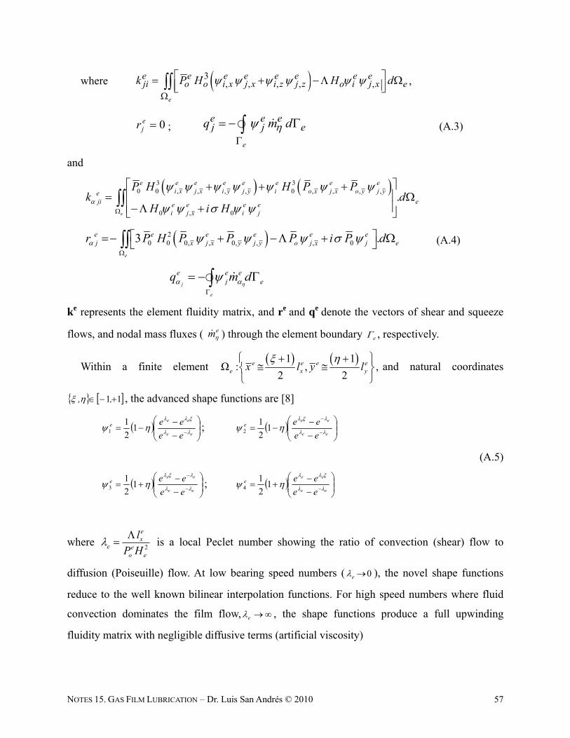
NOTES 15. GAS FILM LUBRICATION – Dr. Luis San Andrés © 2010 57
where 3, , , , ,
e
e e e e e e e eji o o i x j x i z j z o i j x ek P H H d
,
0ejr ;
e
e e ej j eq m d
(A.3)
and
3 3
0 0 , , , , 0 , , , ,
0 , 0
.e
e e e e e e e ei x j x i y j y i o x j x o y j ye
ji ee e e ei j x i j
P H H P Pk d
H i H
20 0 0, , 0, , , 03 .
e
e e e e e ej x j x y j y o j x j er P H P P P i P d
(A.4)
j
e
e e ej eq m d
ke represents the element fluidity matrix, and re and qe denote the vectors of shear and squeeze
flows, and nodal mass fluxes ( em ) through the element boundary e , respectively.
Within a finite element 1 1
Ω : , ,2 2
e e e ee x yx l y l
and natural coordinates
11 ,, , the advanced shape functions are [8]
ee
ee
ee
eee
12
11 ;
ee
ee
ee
eee
12
12
(A.5)
ee
ee
ee
eee
12
13 ;
ee
ee
ee
eee
12
14
where 2
ex
e eo e
l
P H
is a local Peclet number showing the ratio of convection (shear) flow to
diffusion (Poiseuille) flow. At low bearing speed numbers ( 0e ), the novel shape functions
reduce to the well known bilinear interpolation functions. For high speed numbers where fluid
convection dominates the film flow, e , the shape functions produce a full upwinding
fluidity matrix with negligible diffusive terms (artificial viscosity)

NOTES 15. GAS FILM LUBRICATION – Dr. Luis San Andrés © 2010 58
Eq. (A.2) are constructed for each element, assembled over the flow domain, and then
condensed by enforcing appropriate boundary conditions, including the source terms arising
from any external (orifice) pressurization. The resultant global set of equations is
G G GG o o ok P =Q + R (A.6)
where1 1 1
; ;Nem Nem Nem
e e e
G
e e e sourcesG G ok k R r Q q + q for the equilibrium pressure field. A similar
equation set follows for the first-order pressure fields. The asymmetric global fluidity matrix kG
is nonlinear since its elements depend on the zeroth-order pressure field (GoP ).
Earlier developments relied on the continuous evaluation, assembly and decomposition of the
global fluidity matrix. Presently, a line solver with successive under-relaxation is used. The
procedure assembles the finite element equations along a line (constant axial coordinate) and
solves them using the TDMA algorithm. The method is faster than the full matrix decomposition
procedure since new pressures are immediately updated in the iterative procedure. Good
convergence rates are found by selecting appropriate under relaxation factors (0.7 typically).
See Refs. [8-10] for further details on the method implementation, including external
pressurization (supply ports) and tilting pad bearings.