Barbara Tabachnick

http://www.csun.edu/~vcpsybxt/

btabachnick@csun.edu

Not Your Grandma’s Time-Series

Analysis

Statistics WorkshopWestern Psychological Association, April 30, 2015, Las Vegas, Nevada

What is Time Series Analysis?

Data from a single individual over at least 50

time periods

◦ E.g.: weight before and after buying a Fitbit

Data from a group of individuals over at least

50 time periods

◦ E.g.: number of visits to a mental health agency

before and after a major earthquake

What a Time-Series Plot Looks Like

Some Kinds of Time Series Analyses

Effects of an intervention (interruption)

◦ Non-experimental (naturally occurring event)

◦ Quasi-experimental (experimentally-invoked event)

Effects of covariates

◦ E.g.: Does room temperature affect productivity?

Forecasting – what does the future hold?

◦ E.g.: Will thumb drive prices continue to decrease?

Why Bother?

Deal with assumption of independence in

regression (autocorrelation violates

homogeneity of covariance)

Provide a stable baseline against which to

evaluate effects of interventions and covariates

Assumptions and Limitations

Normality of distributions of residuals◦ Take a look at continuous variables (DV and covariates):

if seriously skewed prior to modeling, try out some transformations (e.g., log, square root)

◦ Examine normalized plots of residuals after modeling

Homogeneity of variance and zero mean of residuals (after modeling)◦ Take a look at plot of standardized residuals vs.

predicted values (aka PPLOT): try out some transformations as above.

Will demonstrate post-analysis tests in example

Assumptions and limitations (cont’d)

Independence of residuals

◦ Look at autocorrelation and partial autocorrelation

plots, adjust model if necessary

Absence of outliers

◦ Examine series plot for obvious aberrant points (e.g.,

little blue dot on next plot)

◦ Replace outlier (p<.001)with value one unit

above/below next highest/lowest value for the series

Replacing an outlier with next lowest value

Major Steps in Time-Series Analysis

Identification of best ARIMA model: 3 components

(x, y, z)

Estimation of parameters: ARIMA parameters and

intervention parameters (if any)

Diagnosis of residuals

Interpretation of parameters

Identifying a Model: ARIMA

AR: Autoregressive components – the memory for past observations

◦ AR1 refers to greatest relationship between each observation and the one immediately preceding it, with relationships reducing with observations further back in time (1, y, z)

◦ AR2 refer to greatest relationship between an observation and the one preceding the one immediately preceding it (2, y, z)

Identifying a Model: ARIMA

I: Integrative components – systematic changes in slope or variance of the series. These are dealt with by differencing observations.

◦ I1 refers to a series in which the observations systematically increase and decrease (x, 1, z). A difference score is an observation minus the observation before it.

◦ I2 refers to a series in which the observations are systematically becoming more or less variable (x, 2, z). A double difference is a difference score minus the difference score before it.

00.5

11.5

22.5

33.5

44.5

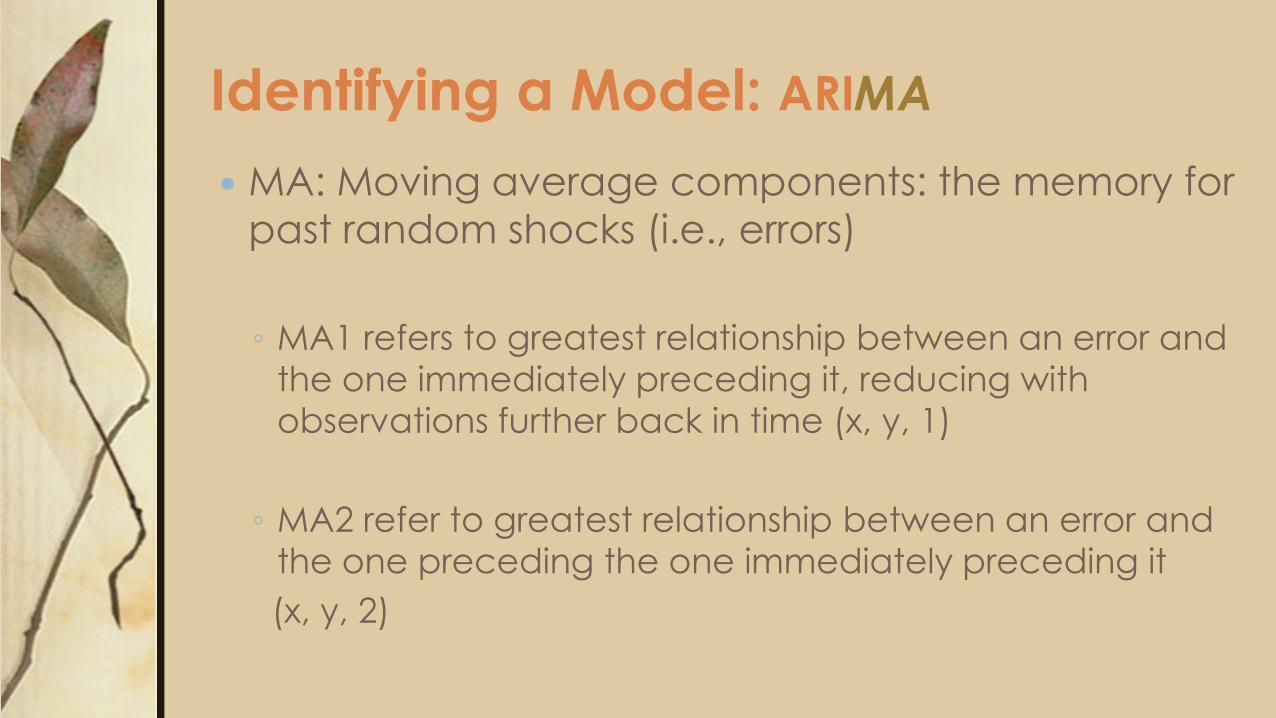
Identifying a Model: ARIMA

MA: Moving average components: the memory for

past random shocks (i.e., errors)

◦ MA1 refers to greatest relationship between an error and

the one immediately preceding it, reducing with

observations further back in time (x, y, 1)

◦ MA2 refer to greatest relationship between an error and

the one preceding the one immediately preceding it

(x, y, 2)

ACF and PACF

ACF = autocorrelation function◦ Correlations with observations at

sequential lags

PACF = partial autocorrelation function◦ Partial correlations (i.e., correlations

with observations at sequential lags with previous correlations partialled out).

Want to end up with all correlations within error bars (confidence limits)

SeasonalityAutocorrelations that are

predictably spaced in

time

For example, monthly

data would be

expected to show spikes

every 12 months

Shown as, for example:

(0, 0, 1)(0, 0, 1)12

Examples of Mixed ARIMA Models

AR1, I1, MA1 (1, 1, 1)

AR1, I0, MA2 (1, 0, 2)

AR0, I1, MA1, weekly data (0, 1, 1)(0, 1, 1)7

Estimation Find parameters of ARIMA model

In grandma’s day, had to visually identify

models (tea leaves) from ACF and PACF

Now can use “expert modelers” available in IBM SPSS and

SAS

If there is an intervention, estimation of ARIMA parameters is

done on data collected before the intervention

Estimate parameters of intervention and/or covariate(s), if

any

Diagnosis

Look at residual ACF and PACF plots to make

sure bars (correlations and partial correlations)

are within confidence limits

Look at residuals through normal probability

plots

Fix problems, if any, and rerun analysis if

necessary

Interpretation

Interpret ARIMA model if that is of research interest

Interpret effect(s) of intervention(s): parameter estimate(s), effect size

𝑅2 = 1 −𝑆𝑆𝑟𝑒𝑠𝑖𝑑𝑢𝑎𝑙 𝑤𝑖𝑡ℎ 𝑒𝑓𝑓𝑒𝑐𝑡

𝑆𝑆𝑟𝑒𝑠𝑖𝑑𝑢𝑎𝑙 𝑤𝑖𝑡ℎ𝑜𝑢𝑡 𝑒𝑓𝑓𝑒𝑐𝑡

Interpret effect(s) of covariates(s): parameter estimate(s), effect size (as above)

Kinds of Interventions (transfer functions)

Indicate intervention by adding a variable that

codes intervention

Abrupt permanent

0 = all pre-intervention times, 1 = all post-intervention

Kinds of Interventions (continued)

Abrupt temporary

0 = all pre-intervention times, 1 = first post-intervention

0 = remaining post-intervention

Kinds of Interventions (continued)

◦ Gradual

◦ permanent temporary

Kinds of Interventions (continued)

◦ Multiple interventions: add a variable for each

intervention, then code each as above

Sample Data Dr. Debbie Denise Reese. CyGames Selene

educational game: create the moon, learn lunar

science http://selene.cet.edu/default.aspx?page=Selene

Does implementation of a Dashboard increase player

persistence?

Sample Data (cont’d) Data collected for 194 weeks: 181 before dashboard implementation,

13 weeks after. Looking for increase in persistence (DV) with introduction of dashboard

Data aggregated over all players for each week

Covariate added to reflect proportion of Spanish-language players because of one hugely successful classroom of Spanish players after implementation of dashboard

Initial data screening revealed extreme positive skewness for persistence (DV) and proportion speaking Spanish so each transformed logarithmically

Data screening revealed a few outliers in persistence. They were replaced with values .01 greater or less than next most extreme value

Data File Showing Intervention and

Covariate Codes

IBM SPSS runs: Initial look at Series

Analyze >

Forecasting >

Sequence Charts…

Initial look at Series (menu and pasted syntax)

Note that Persistence is

variable name but label is

Log10(Persistence + 1). No log

transform of DV because already

Done.

Initial look at Series (selected output)

Red line added manually

to indicate intervention

No evidence of seasonality

Ideally should have more post-

intervention data, but grant ended.

Initial Look at ACF and PCF: input

Analyze>

Forecasting>

Autocorrelations…

Initial Look at ACF and PCF: input (cont’d)

Initial Look at ACF and PCF: output

Identify ARIMA Model: Limit data to pre-

intervention cases

Data > Select Cases… >

If condition is satisfied > If…

Identify ARIMA Model: Input

Analyze > Forecasting > Create Models…

Identify ARIMA Model: Input (cont’d)

Identify ARIMA Model: Input (cont’d)

Model Identification: Output

IBM SPSS chooses (2, 0, 1) model

Residual plots not

optimal but no better with

other models attempted

Include Post-intervention Cases for

Estimation

Data > Select Cases… >

All cases

Parameter Estimation with All Cases

Analyze > Forecasting > Create Models…

Parameter Estimation: menu choices

Add Intervention

(dashboard) to model

Select ARIMA as

Method

Select Criteria

Parameter Estimation: criteria

Define (2, 0, 1) model

Parameter Estimation: statistics

Parameter Estimation: plots

Parameter estimation: save residuals

Residuals are added to data

Set (for PPLOT, later)

Parameter Estimation: syntax and output

Fit statistics will

be used to

calculate effect

size (later)

Parameter Estimation: output (cont’d)

Dashboard is a significant predictor of persistence. Covariate (Proportion Spanish-

speaking) is not.

Parameter estimate for Dashboard Log of Persistence is .218. Antilog is 10.218 = 1.65.

There is a 65% increase in persistence after introduction of the dashboard. Using

untransformed persistence data (in file as Persistence_Raw, but not shown), splitting the

file on dashboard:

median for pre-dashboard = 14.7; median for post-dashboard = 24.2.

Initial interpretation:

Note for later: number of parameters = 6 (including constant)

Effect Size: menu and syntax

Calculation of the effect size for Dashboard requires another model run (just like

Parameter Estimate run, but with Dashboard omitted).

Effect Size: (cont’d)

RMSE without Dashboard = .194

RMSE with Dashboard = .190

RMSE is a standard deviation

SS = df(variance) = df(RMSE)2

df – N – (number of parameters including constant)

df = 194-5* = 189

df = 194-6 = 188

SS = df(RMSE)2

= (189)(.194)2 = 7.11

SS = df(RMSE)2

= (188)(.190)2 = 6.78

𝑅2 = 1 −𝑆𝑆𝑤𝑖𝑡ℎ 𝑑𝑎𝑠ℎ𝑏𝑜𝑎𝑟𝑑

𝑆𝑆𝑤𝑖𝑡ℎ𝑜𝑢𝑡 𝑑𝑎𝑠ℎ𝑏𝑜𝑎𝑟𝑑= 1 −

6.78

7.11=.046

*Dashboard (df=1) omitted

Model Diagnosis: residual ACF and PACF

From major estimation output with Dashboard included

Model DiagnosisFrom major modeling output with Dashboard included

Model Diagnosis: PPLOT (AVAILABLE ONLY IN SYNTAX)

PPLOT NResidual_Persistence_Model_1

/distribution=NORMAL

/plot=both.

Looks like outlier in upper right.

Finding the Outlier Save file under new name

Sort by “NResidual_Persistence_Model_1” (this is a variable

produced by requesting that residuals be saved)

Data >

Sort Cases…

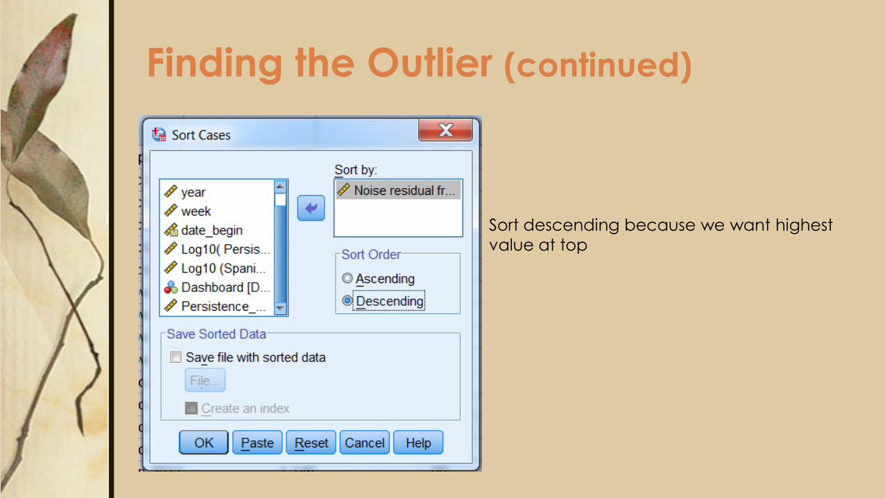
Finding the Outlier (continued)

Sort descending because we want highest

value at top

Finding the outlier (continued)

1. Resave file with new name

2. Re-sort by DV (persistence)

3. Change persistence score for

Weekly Count 157. Insert 1.720

(to replace 1.957).

3. Rerun entire analysis

Results of Re-AnalysisIdentification remains the same: (2, 0, 1)

Fit improved:

RMSE reduced from .190 to .184

Parameter Estimation: reanalysis

As before, Dashboard is a significant predictor of persistence. Covariate (Proportion

Spanish-speaking) is not.

Parameter estimate for Log of Persistence is .224. Antilog is 10.224 = 1.67.There is a

67% increase in persistence after introduction of the dashboard – very slight

increase from initial analysis..

Using untransformed persistence data (in file, but not shown), splitting the file on

dashboard: median for pre-dashboard = 14.7; median for post-dashboard = 24.2.

interpretation: Model fits much better—cleaner results

Reanalysis of Effect Size of Dashboard

RMSE without Dashboard = .192

df = 194-6 = 188

RMSE with Dashboard = .187

SS = df(RMSE)2

= (189)(.188)2 = 6.68

SS = df(RMSE)2

= (188)(.184)2 = 6.36

df = 194-5 = 189

RMSE is a standard deviation

SS = df(RMSE)2

df – N – (number of parameters including constant)

𝑅2 = 1 −𝑆𝑆𝑤𝑖𝑡ℎ 𝑑𝑎𝑠ℎ𝑏𝑜𝑎𝑟𝑑

𝑆𝑆𝑤𝑖𝑡ℎ𝑜𝑢𝑡 𝑑𝑎𝑠ℎ𝑏𝑜𝑎𝑟𝑑= 1 −

6.36

6.68=.048

Little change

Re-Diagnosis: residual ACF and PACF

Better than with outlier

(all bars within 95% CL)

Diagnostic PPlots – outlier removed

Re-Analysis Final Summary Plot