Embed Size (px)
Citation preview

Norwegian Wind Power: Levelized production costs and grid parity
Ben-Frode Bjørke
Master thesis at the Department of Economics
UNIVERSITETET I OSLO
31.08.2009

ii

iii
Preface
This thesis has been written during the first half of 2009. The purpose of this work has been to
study the long-run marginal cost and grid parity for Norwegian wind power.
I would like to thank my supervisor Steinar Strøm for great advices and discussions.
Thanks to the Norwegian Wind Energy Association (NORWEA) for providing financial
support and data. A special thanks to Secretary General Øyvind Isachsen for having
confidence in me from day one.
I would also like to thank Trond Jensen at Statnett for his support on the BID-model (and of
course the cycling conversations).
Thanks to Øistein Schmidt Galaaen for proof reading and feedback.
And finally, thank you May-Liss. We did it!
Errors and weaknesses in this thesis are the author’s responsibility.
Ben F. Bjørke
Oslo, August 2009

iv
Table of contents
Preface ....................................................................................................................................... iii
1. Introduction ............................................................................................................................ 1
2. Renewable energy: How the focus emerged .......................................................................... 3
2.1 The regulation period ....................................................................................................... 3
2.2 Liberalization of the energy market ................................................................................. 4
2.3 New renewable energy ..................................................................................................... 6
2.4 Environmental issues ........................................................................................................ 7
3. Policies for promoting the development of wind power ........................................................ 9
3.1 A closer look at the Norwegian model ............................................................................. 9
3.2 Support schemes to renewable energy ........................................................................... 12
3.2.1 Green certificates ..................................................................................................... 12
3.2.2 Feed-in tariffs .......................................................................................................... 12
3.2.3 Competitive bidding process ................................................................................... 13
4. The European power sector .................................................................................................. 15
4.1 The development of wind power in the EU and Norway ............................................... 15
4.2. Capacity Development of wind turbines in Europe and Norway .................................. 17
5. Modeling wind power in a closed economy ......................................................................... 22
5.1 Competitive markets and economic efficiency .............................................................. 22
5.2 An equilibrium model with hydro and wind power ....................................................... 24
5.3 Cost calculation methodology ........................................................................................ 25
6. Costs of wind energy ............................................................................................................ 27
6.1 Capital cost break down ................................................................................................. 27
6.1.1 Turbine supply agreement (TSA) ............................................................................ 29
6.1.2 Electrical costs ......................................................................................................... 30
6.1.3 Civil cost ................................................................................................................. 30
6.1.4 Development and planning costs ............................................................................. 30

v
6.1.5 Contingency ............................................................................................................ 31
6.2 Variable costs ................................................................................................................. 31
6.2.1 Operation and maintenance costs ............................................................................ 31
6.3 Wind energy output ........................................................................................................ 33
6.4 The Discount Rate .......................................................................................................... 36
6.4.1 The Capital asset pricing model .............................................................................. 37
6.4.2 What is the right level of the discount rate? ............................................................ 38
6.5 Other cost components ................................................................................................... 39
6.5.1 External costs .......................................................................................................... 39
6.5.2 Economic lifetime ................................................................................................... 40
6.5.3 Salvage value ........................................................................................................... 40
6.6 Long-run marginal cost curve ........................................................................................ 40
6.7 Uncertainties ................................................................................................................... 41
6.7 Costs: A closer look at specific wind sites in Norway ................................................... 43
6.7.1 Cost components reassessed .................................................................................... 43
6.7.2 LPC-assessment of Norwegian wind power plants ................................................. 44
7. Price scenarios ...................................................................................................................... 47
7.1 The liberalized electricity market ................................................................................... 47
7.2 Price variations in the perfect competitive market ......................................................... 49
7.3 Future price scenarios ..................................................................................................... 51
8. Grid parity and future cost development .............................................................................. 55
8.1 Grid parity ...................................................................................................................... 55
8.2 Future cost development ................................................................................................ 56
9. Concluding remarks ............................................................................................................. 58
References ................................................................................................................................ 60
Appendix A .............................................................................................................................. 62

1
1. Introduction
Indeed, wind power is about to play a major role in the European transition to a more climate
friendly production of energy, reducing the need for conventional energy production and the
threat to energy security. During the last 20 years the wind power generated output has
increased to more than 100 TWh from the small 0,7 TWh, most of it in countries like
Denmark, Germany and Spain. But in several other countries the wind power development is
ready for departure and among these countries we find Norway. In 2000, ten years after the
enactment of the new Energy Act, which laid the legal foundation for the liberalization of the
Norwegian electricity market, the target of 3 TWh annual production of wind energy by 2010
was launched. The ambitious target was accompanied by the establishment of the public
company Enova, which responsibility was to ensure domestic wind energy investments and
provide financing through the new Energy Fund.
For wind power, like all other new renewable energy sources, the long-run marginal cost
exceeds the market price. In a liberalized competitive market we would expect to see
investments if and only if the long-run marginal cost equated the market price. In other words,
we should not expect any new investments in wind energy as long as the competitive market
principle is not fulfilled. However, the rapid development of wind power and the
establishment of public financial institutions like Enova underscore the political will to
subsidize the wind industry. Given that society finds it important to invest in wind power, it is
important to acquire knowledge about the magnitude of the subsidy in the future. Even though
society chooses to support wind power financially, it is in society’s best interest to minimize
the subsidy. The main purpose of this thesis is to study the grid parity of Norwegian wind
power. Grid parity is defined as the point at which the cost of electricity from wind power will
equal the cost of producing electricity by traditional means without taking into consideration
subsidies. For a technology to reach its grid parity either the market price must increase or the
long-run marginal cost decrease. By estimating future energy prices, information about the
future price development can be obtained. By identifying the cost components and estimate
their value, calculation of the long-run marginal cost is obtained. Comparison of the two will
provide information on whether or not Norwegian wind power will reach its grid parity,
hence, if there will a need for subsidies in the future.
The wind power industry is capital intensive, as much as 75 to 80 percent of the total cost is
related to upfront capital costs while the operation and maintenance cost attribute to the

2
remaining 20 to 25 percent. Further, the wind turbine cost attributes to approximately 70-80
percent of the total capital cost, which means that any future cost decrease in large part must
come from the turbine producers or more efficient turbines. The information from the capital
and operational and maintenance cost breakdown has been used to calculate the long-run
marginal cost for 12 of the Norwegian wind farms which have gotten their application for
concession approved by the energy authorities. The long-run marginal cost, also referred to as
the levelized production cost (LPC), is calculated in range between approximately 0,5
NOK/kWh and 0,7 NOK/kWh with a discount rate of 6 percent. In order to estimate the future
price development, a scenario for 2025 has been developed. The future price is estimated by
the use of the BID-model for Norway and the neighboring trade partners, and is for Norway
reported at an average NOK 0,33.
It then remains to see whether or not it is reasonable to expect the cost of wind power to
decrease. Studies of experience curves show that the turbine price is expected to decrease
between 2 to 8 percent when the cumulative production doubles (Neij et al., 2003).
The rest of the thesis is organized as follows: In Chapter 2, a brief review on how wind power
entered the Norwegian political agenda is provided. Chapter 3 describes the policies for
promoting the development of wind power, with emphasis on the Norwegian model for
subsidies. Chapter 4 describes the development of wind power and other energy sources in
EU27 and Norway. In Chapter 5 an equilibrium model with hydro power and wind power is
presented, as well as cost calculation methodology. Chapter 6 describes the components of the
costs related to wind power and calculates the levelized production costs for 12 Norwegian
wind farms. The discount rate and the annual energy output have a major impact on the level
of the LPC, and the chapter provides a thorough discussion on the two factors. Chapter 7 uses
scenario methodology to estimate future electricity market prices for five of the Norwegians
price regions and the neighboring trade partners (reported in the Appendix). Chapter 8
establishes a Salter-diagram which illustrates that the Norwegian wind power industry has yet
to reach its grid parity. It also briefly discusses the future development of wind power costs.
Chapter 9 concludes the thesis.

3
2. Renewable energy: How the focus emerged
The main purpose of this chapter is to provide an overview of how the focus on new
renewable energy in Norway emerged. The chapter looks at the regulation period – the time
period from the 1950s to the end of the 1980s, and the deregulation of the Norwegian energy
market through the introduction of the Energy Act of 1990. The chapter then briefly considers
some environmental issues in regard to wind power.
2.1 The regulation period
The Energy Act of 1990 laid the legal foundations for the Norwegian energy market reform.
The main motivation for the reform was an increasing dissatisfaction with the performance of
the sector in terms of economic efficiency in resource utilization, particularly in regard to
investment behavior, which caused capacity to exceed demand (Bye & Hope, 2005). To reach
the socially optimal development of power plants, the plants should be ranked according to
their long run marginal costs and no projects should be developed before the long run
marginal cost equated the market price.
Historically, there has been no direct link between market prices and investment. During the
regulation period, all investments in production and transmission capacity were subject to cost
reimbursement. In the years before 1979 government equated average costs to prices.
Investment decisions were based on energy prognoses provided by the government and in
principle any increase in demand should be covered by increasing supply. This led to
overinvestment in power production.
In 1979 a new pricing rule was implemented. Now the investment decisions should be based
on the long run marginal cost principle (see Chapter 5). In a free market the marginal cost
principle says that investment can take place when the price equals long run marginal costs.
However, during the 1980s prices were still regulated by the government. The government
used the long run marginal cost as a price criterion rather than an investment decision rule.
The result was inefficient utilities and output maximization to ensure adequate supply. In
addition different prices were set for different consumers, which led to inefficiencies and
welfare losses. Bye & Hope (2005) points to Midttun (1987) to outline the political discussion
on investment and pricing in Norway during the 1960s to 1980s. Midttun’s conclusions
include the following: (i) Production capacity in state-owned companies had not increased
following increases in marginal costs. (ii) The power price had never been high enough to

4
cover the marginal cost of expansion. (iii) The expansion of capacity had led to excessive
investments. After 1979, when the investment rule of equating prices to marginal costs was
introduced, politicians wanted to lower the discount rate on investment projects to secure
lower prices.
It is obvious that throughout the whole regulation period, politicians tried to avoid higher
electricity prices. They wanted to keep prices stable and planned investment from a goal of
having stable prices. Inefficiencies in transmission and distribution and inefficiencies in the
market were other market imperfections that were identified during the regulation period, see
Bye & Hope (2005, p.7–8) and Bye & Halvorsen (1998).
2.2 Liberalization of the energy market
A full opening of the Norwegian electricity market was carried out through the introduction of
Act no. 50 of 29 June 1990: Act relating to the generation, conversion, transmission, trading,
distribution and use of energy etc. The purpose of the act is given in Section 1-2: The Act
shall ensure that the generation, conversion, transmission, trading, distribution and use of
energy are conducted in a way that efficiently promotes the interests of society, which
includes taking into consideration any public and private interests that will be affected. Bye &
Hope (2005) highlights the main elements of the Norwegian electricity market reform:
• The market was designed to be a regular spot market incorporating demand. The
market was immediately open to all potential buyers, including households.
• Common carriage principles requiring access to the network system on a transparent
and nondiscriminatory basis facilitated market-based trade.
• The state-owned giant Statkraft was split vertically into two separate legal entities:
The generating company, Statkraft SF, and the transmission company, Statnett SF.
Other vertical integrated companies were split into generating or trading divisions and
network divisions.
• The network companies were subject to natural monopoly regulations designed to
achieve economic efficiency in network operations. In 1997, income frame regulations
were introduced instead.
• Privatization of the power sector was politically unacceptable. Therefore the market
liberalization reform was implemented without changes in ownership.

5
The deregulation of the market was expected to lower investment, reduce and equalize prices
between consumers, lower net tariffs, and raise the rate of return on investment.
During the regulation period the public attempted to equate prices to long-run marginal costs.
Theoretically, long-run prices should then reflect long-run marginal costs, and excess capacity
should not be possible. However, during the regulation period excess capacity was the case.
One of the reasons was that the energy-intensive industries paid prices corresponding to 25
percent to 33 percent of the long-run marginal costs. Prices were set to match the energy-
intensive industry’s competitiveness and not from the alternative value in the market. Another
reason was that excess production in relation to domestic demand was sold on the
international market in the form of occasional power at low prices. The producers could then
keep prices relatively high in the domestic market and sell the excess production on the
international market. A third reason for excess capacity was the spilling of up to five per cent
of the inflows during the periods of spring melting and fall rains. A fourth argument was that
there did not exist a ranking of the not-developed projects. Finally, when the new marginal
cost pricing rule was introduced in 1979, the electricity tax was included in the long-run price.
Hence, the long-run prices were in fact lower than faced by the investors.
Due to the deregulation of the Norwegian electricity market, previously excess capacity
competes in the market. When excess capacity competes in the market, electricity prices are
below long-run marginal costs in the short and medium run. This persists until demand
increases and production capacity constrains growth. Then prices increase again and stimulate
further investment. The deregulation also put a downward pressure on prices by generating an
expected efficiency gain in terms of operating costs and investment costs. Finally, it led to
price equality between consumers.
During the regulation period and the first six years after the 1991-deregulation, Norway was a
net exporter of electricity. But investments in new production had already started to decline in
the early 1980s. This was mainly because of a sharp increase in the marginal cost of
expansion and environmental concerns (Bye and Hope, 2005). After deregulation, investment
continued to fall. On the other hand, demand increased, Norwegian capacity was restricted
and prices increased. In his new year’s speech in 2001, the Norwegian prime minister outlined
that new investments in large hydro power is over. Since then politicians have seemed
unanimous in the blocking of new investments in hydro, nuclear and other thermal plant
6
technologies. The only feasible alternatives seem to be new renewable technologies like solar,
biomass, wave, and on- and offshore wind energy.
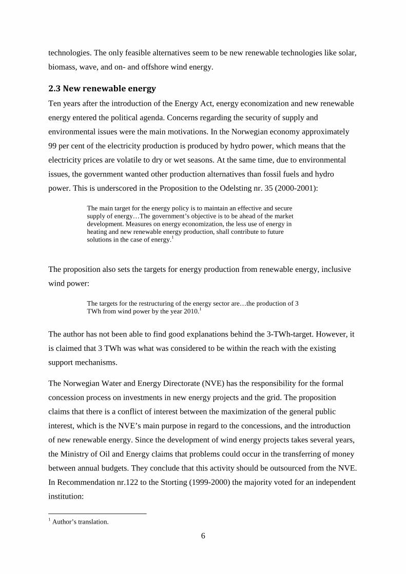
2.3 New renewable energy
Ten years after the introduction of the Energy Act, energy economization and new renewable
energy entered the political agenda. Concerns regarding the security of supply and
environmental issues were the main motivations. In the Norwegian economy approximately
99 per cent of the electricity production is produced by hydro power, which means that the
electricity prices are volatile to dry or wet seasons. At the same time, due to environmental
issues, the government wanted other production alternatives than fossil fuels and hydro
power. This is underscored in the Proposition to the Odelsting nr. 35 (2000-2001):
The main target for the energy policy is to maintain an effective and secure supply of energy…The government’s objective is to be ahead of the market development. Measures on energy economization, the less use of energy in heating and new renewable energy production, shall contribute to future solutions in the case of energy.1
The proposition also sets the targets for energy production from renewable energy, inclusive
wind power:
The targets for the restructuring of the energy sector are…the production of 3 TWh from wind power by the year 2010.1
The author has not been able to find good explanations behind the 3-TWh-target. However, it
is claimed that 3 TWh was what was considered to be within the reach with the existing
support mechanisms.
The Norwegian Water and Energy Directorate (NVE) has the responsibility for the formal
concession process on investments in new energy projects and the grid. The proposition
claims that there is a conflict of interest between the maximization of the general public
interest, which is the NVE’s main purpose in regard to the concessions, and the introduction
of new renewable energy. Since the development of wind energy projects takes several years,
the Ministry of Oil and Energy claims that problems could occur in the transferring of money
between annual budgets. They conclude that this activity should be outsourced from the NVE.
In Recommendation nr.122 to the Storting (1999-2000) the majority voted for an independent
institution:
1 Author’s translation.

7
The majority points out that the NVE should be relieved from the task of coordination and clarification in regard to supporting…energy production. On this background the majority proposes the establishment of a new state-owned company…The (company’s) objective should be to reach the targets set within electricity economization, the transition from electricity to heat, and wind power.2
This provides the fundament for the establishment of the state-owned company Enova SF,
which was established in 2001. Through Recommendation nr.59 to the Odelsting (2000-
2001), Enova’s mandate was to coordinate the reformation of energy usage and design a new
financing model suited for the introduction of wind power and other renewable energy
sources. Enova SF was also handed the responsibility for a new energy fund, established
January 2002, and to increase the production of energy from wind power with 3 TWh, starting
in 2000. The regulation responsibilities for the Energy Fund were handed to the Ministry of
Oil and Energy. The fund should support and ensure that assets were used in a productive way
as possible for providing predictable financial support in the advantage of investments in
renewable energy. The fund was financed through the grid tariff, which at the date of
establishment was 0,3 Nøre/kWh. From July 2004 the tariff increased to 1 Nøre/kWh, which
implies approximately an annual tax increase of NOK 200 for a household that consumes
20000 kWh per year3. The Energy Fund also finances the operational cost for Enova SF.
2.4 Environmental issues
Besides energy supply issues, the environmental concerns have been the primary argument for
the investment in, and transition into, low carbonized energy production. One of the major
papers on the environmental issue is the Stern Review on the Economics of Climate Change
released in October 2006. Although not the first economic report on climate change and
global warming, it is significant as the largest and most widely known and discussed of its
kind. According to Stern (2006) climate change is the greatest and widest-ranging market
failure ever seen. To be able to cope with the increasing emissions of CO2 the power sector
around the world will have to be at least 60 percent, and perhaps as much as 75 percent,
decarbonised by 2050 to stabilize at or below 550ppm CO2e4. Three elements of policy for
mitigation are essential: A carbon price, technology policy, and the removal of barriers to
behavioral change.
2 Author’s translation. 3 The Norwegian average electricity consumption is 20000 kWh per year. 4 Carbon Dioxide Equivalence (CO2e) is a quantity that describes, for a given Greenhouse Gas, the amount of CO2 that would have the same global warming potential, when measured over a specified timescale (generally, 100 years).
8
While many of the technologies to achieve this already exist, such as wind power, the priority
must be to bring down their cost so that they can compete with fossil-fuel alternatives under a
carbon-pricing policy regime (Stern, 2006). The social cost of carbon is likely to increase
steadily over time because marginal damages increase with the stock of green house gases in
the atmosphere, and that stock rises over time. This should foster the development of
technology that can drive down the average cost of abatement. However, pricing carbon, by
itself, will not be sufficient to bring forth all the necessary innovation, particularly in the early
years. The development and deployment of a wide range of low-carbon technologies is
essential in achieving the deep cuts in emissions that are needed. Experience shows that costs
of technologies fall with scale and experience. Carbon pricing gives an incentive to invest in
new technologies to reduce carbon. Indeed, without it, there is little reason to make such
investments. But investing in new lower-carbon technologies involves risk. Companies may
worry that they will not have a market for their new product if carbon-pricing policy is not
maintained into the future. And the knowledge gained from research and development is a
public good; companies may under-invest in projects with a big social payoff if they fear they
will be unable to capture the full benefits. Thus there are good economic reasons to promote
new technology directly. Policies to support the market for early-stage technologies will be
critical. Different support schemes for the promotion of renewable energy will be discussed in
Chapter 3. The investments made in the next 10-20 years could lock in very high emissions
for the next half-century, or present an opportunity to move the world onto a sustainable path.
Calculations based on income, historic responsibility and per capita emissions all point to rich
countries taking responsibility for emissions reductions of 60-80 percent from 1990 levels to
2050.
Markets for low-carbon energy products are likely to be worth at least $500bn per year by
2050, and perhaps much more. According to the Stern-review (2006), individual companies
and countries should position themselves to take advantage of these opportunities.

9
3. Policies for promoting the development of wind power
Due to high fixed costs, low running costs and a fairly long lifetime, economics of wind
turbines have not yet reach its grid parity. Hence, wind power is highly dependent on stable
and long-term agreed payments for the turbine’s electricity production. Characteristic for the
three top wind energy producing countries, Germany, Spain and Denmark, is that they have
introduced long-term agreements on fixed feed-in tariffs, and that these feed-in tariffs are
fixed at relatively high levels. It seems like the introduction of the standard payment schemes
has had a significant influence on the wind turbine development in these countries (Morthorst,
1999a). Denmark, Germany and Spain together cover more than 80 percent of the total
European wind energy capacity. Norway, on the other hand, was part of green certificate
regime with Holland until the beginning of 2003, when Holland withdrew from the
agreement. Then Norway introduced a competitive bidding incentive scheme, which in terms
of absolute capacity growth has proved less effective (Menanteau et al., 2003).
During the past few years, a number of different policy instruments have been used to
promote the development of wind power. In addition to carbon and energy taxes on the
production from conventional energy supply technologies, these instruments or support
schemes fall into three main categories that are either price-based or quantity-based:
• Feed-in tariffs, used particular in Germany, Spain and Denmark.
• Bidding processes, such as the one used in Norway.
• Tradable green certificates schemes, where electricity suppliers are obliged to produce
or distribute renewable energy. This type of instrument is used in Sweden, but could
eventually be extended to all European countries (Menanteau et al., 2003).
This chapter deals with the three incentive schemes, though with a more thorough description
of the Norwegian model.
3.1 A closer look at the Norwegian model
One of the objectives of the establishment of Enova was to establish a more cost effective
approach to new renewable energy. In order to decide which wind power plant to receive
support, Enova ranks the different projects according to energy results, defined as NOK/kWh,
the projects economical lifetime and the target of 3 TWh wind power by 2010. Generally
projects with low costs relative to generated effect will by definition be competitive by
themselves and not receive payments from the Energy Fund.

10
In 2002 Enova released its investment support scheme for wind power. In addition a program
for the benefit of research on wind power was introduced. The investment support scheme
provides a maximum of 20Nøre/kWh per year, limited to a maximum of ten per cent of
approved investment costs set to max six million NOK per MW installed capacity.
The Enova support shall not over-compensate the wind projects. The policy shall trigger
investments, which means that the project would not be started without the support from
Enova. The term over-compensation means that the project shall not receive a larger relative
economical support than what is needed in order to construct the wind farm. The investment
support is based on the project’s net present value analysis, including the project’s expected
rate of return or discount rate. Enova bases its decision on the following factors:
• A discount rate of 8 percent.
• The lifetime, given as construction time plus 20 years of production.
• Electricity prices, based on the six monthly three years forward on the Nord Pool
given at the date of appliance.
• Income, calculated from the electricity price multiplied by expected production.
• Exchange rate at the date of appliance.
In addition the project must provide a climate report, including documentation on all
environmental implications, a tentative offer from the turbine company, including total costs
and type of turbine, a statement from the grid company on excess grid capacity and a project
description which includes capital investment costs, operating costs, tentative financial plan
and a plan of progress. The projects are then evaluated from two main criteria: (i) The projects
financial plan and the size of needed economical support and (ii) project costs in relation to
the energy result (kWh).
A new model for financing the Energy Fund was introduced in 2004. From being financed
through the national budget, the new model introduced a mark up on the grid tariff. This mark
up was set to 1Nøre/kWh, which provides the Energy Fund with approximately 650 million
Norwegian kroner per year.
Enova is obliged to document the achievements and does that through the release of a yearly
report. In 2003 the contracted wind power result was 450 GWh and the total support value
NOK 92 million. In 2004 the 1023 GWh wind power was contracted upon, and the total
support value was NOK 384 million. I 2005 the reported level of production for 2004 fell to

11
650 GWh, while the contracted wind power capacity for 2005 was 585 GWh. The reported
value for 2003 in 2005 fell to 124 GWh. In 2006 no support to wind power was given. In
2007 NOK 218 million subsidized 260 GWh of wind power capacity. I 2008 wind power was
subsidized with NOK 445 million, with an estimated production of 276 GWH. In 2009 the
results for 2008 were changed to NOK 93 million and 65 GWh. Obviously the energy results
differ from year to year. The projects given support at a given date are not obliged to start
construction and have the right to reject the support and reapply at a later date. Usually the
reason for rejection has been that the projects have disagreed in the amount of support given.
In 2006 no support was given due to uncertainty regarding future support schemes. At that
time Sweden and Norway discussed the possibility of a mutual Norwegian-Swedish green
certificate market. The Norwegian government concluded that a common certificate market
would become too expensive for the Norwegian consumers and industry and wanted instead
to improve the already established instruments.
Owner District
Support
mill.NOK GWh Year Status Project
Smøla Statkraft Energi AS Smøla 72 120 2001 In operation
Sandhaugen Norsk Miljøkraft AS Tromsø 2,9 4 2003 In operation
Nygårdsfjellet Narvik Energi AS Narvik 4,2 24 2003 In operation
Hundhammerfjellet
Nord-Trøndelag
Elektrisitetsverk Nærøy 35 10 2003 In operation
Hitra Hitra Vind AS Hitra 33,2 155 2003 In operation
Smøla Statkraft Energi AS Smøla 66,6 330 2003 In operation
Hundhammerfjellet NTE Nærøy 65 150 2004 In operation
Valsneset Trønderenergi Kraft Bjugn 30,7 35 2004 In operation
Bessakerfjellet Trønderenergi Kraft Roan 100 155 2005 In operation
Gartefjellet Kjøllefjord Vind AS Lebesby 86 150 2007 In operation
Mehuken 2 Kvalheim Kraft Vågsøy 93 65 2008
Under
construction
Høg Jæren Jæren Energi Time og Hå 511,6 200 2009 Contracted
Fakken Troms Kraft Karlsøy 346,4 200 2009 Contracted
Hundhammerfjellet 2 NTE Nærøy 16,4 10 2009 Contracted
Nygårdsfjellet 2 Nordkraft Vind Narvik 200,1 123 2009 Contracted
Sum 1663,1 1731
Table 3.1: Wind energy results 2001-2009 (Source: Enova).
Table 3.1 sums up the wind energy results for the period 2001-2009. Only projects in
operation, under construction or under contract with Enova are enlisted. During the period

12
2001-2009 a total of 1731 GWh of wind power have received support, with the total value of
NOK 1663 million. In summary, the amount paid per GWh is approximately NOK 1 million.
3.2 Support schemes to renewable energy
The following sections describe the incentive schemes most used within the European energy
market.
3.2.1 Green certificates
The main characteristics of a green certificate market are the following: All consumers are
obliged to buy a certain share of their total electricity consumption from renewable energy
technologies. All renewable energy technologies, including wind power, biomass and biogas
plants, photovoltaics, wave power, geothermal and small hydro plants, will be certified for
producing green electricity5. Per unit (kWh) of electricity produced they will receive a green
certificate, which can be sold to distribution companies or other electricity consumers with the
obligation to cover a share of their electricity consumption with green power. The market will
function solely as a financial one restricted only by the upper limit of green certificates, which
cannot exceed the amount of electricity produced by the renewable technologies.
3.2.2 Feed-in tariffs
The feed-in tariff scheme involves an obligation on the part of electric utilities to purchase the
electricity produced by renewable energy producers in their service area at a tariff determined
by the public authorities and guaranteed for å specific period (Menateau et al., 2003). The
electricity that is generated is bought by the utility above market price. For example, if the
market price for electricity is 0,35 NOK/kWh, then the rate for green power might be 0,8
NOK/kWh. The difference is spread over all the customers of the utility. If NOK 10000 worth
of green power is bought in a year by a utility that has 500000 customers, then for each
customer NOK 0,02 per kWh is added to the electrical bill annually. In a feed-in tariff system
the producers of renewable energy (i.e. wind power) are encouraged to exploit all available
generating sites until the marginal cost of producing wind power equals the feed in tariff. If
the feed in tariff is set to ���, the amount then generated corresponds to ���� (see Fig. 3.1).
Generally, the long-run marginal cost curve is not known, hence the amount generated is
uncertain a priori.
5 The definition of renewable energy is based on the Swedish Proposition to parliament 2002/02:40 (see Flagstad et al., 2004, p. 15).

13
Fig. 3.1: Feed-in tariff (Source: Menanteau et al., 2003).
All projects with a long-run marginal cost less or equal to the tariff will benefit from this kind
of incentive regime. The difference in quality of various sites leads to the attribution of a
differential rent, to the advantage of those projects with the lowest production costs. The
overall costs of reaching the objective is given by the area ��� × ����. From Figure 3.1 we see
that the higher the feed-in tariff, the higher the quantity of wind power generated, and of
course the higher the total cost.
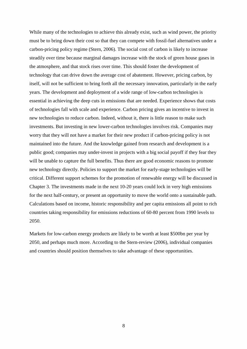
3.2.3 Competitive bidding process
Through the competitive bidding processes, the regulator defines a target for the amount of
renewable energy to be faced in, and organizes a competition between renewable producers to
reach this target. This instrument has been in use in Norway since the establishment of Enova
in 2001, but it has also been applied in the UK and France. The competition focuses on price
per kWh and through their bids the competitors reveal their long-run marginal cost curves (ex
post). It is Enova’s, or the respective countries energy authority’s, task to classify the bids in
increased order until the amount to be contracted is reached.
The amount to be reached is ��� (Fig. 3.2). The marginal cost, ����, is the price for the last
unit of wind power that enables the target to be reached. The implicit subsidies attributed to
each generator correspond to the difference between the bid price and the wholesale market
price. In the competitive bidding system the exact amount of wind power concerned by the
bids is a priori known. However, the marginal cost curves are not known a priori, hence the
total cost of reaching the target cannot be determined. Theoretically, the overall costs of
reaching the target is given by the area situated under the marginal cost curve. Compared to
feed-in tariffs the differential rent paid to renewable energy generators, does not have to be
Quantity ����
���
Price MC
14
borne by the consumers over the electricity bill. It is worth noting that in the Norwegian
regime a tariff of 1 Nøre is added to the electricity bill in order to contribute to the so called
renewable energy fund controlled by Enova.
Fig. 3.2: The Competitive bidding process (Source: Menanteau et al., 2003).
Quantity ���
����
Price MC

15
4. The European power sector
All though the total gross energy generation in Europe (EU27) has grown with 30 percent
during the last 20 years, the composition of the power output has changed. Especially, there
has been a transition from oil-fired power plants to natural gas-fired plants, and renewable
energy has started to play a more important role in the energy composition.
This section investigates the capacity development in the European energy sector for the
period 1990 to 2007. First it looks at the composition of the power output and how this
composition has developed during the time period. Then it focuses on the development of
wind power production. The development within the largest European wind generation
countries will be discussed and the driving forces behind this development will be described.
Norwegian electricity generation will also be discussed and the development of wind power in
Norway will be described.
4.1 The development of wind power in the EU and Norway
As expected the total gross generation of electricity in the EU has increased at an average
annual growth rate of 1,5 percent (see Table 4.1) to 3362 TWh in 2007 from 2854 TWh in
1990. For the whole time period the increase in electricity generation has been 30 percent.
1990 1991 1992 1993 1994 1995 1996 1997 1998 1999 2000 2001 2002 2003 2004 2005 2006 2007
TWh 2584 2628 2617 2617 2655 2733 2830 2841 2910 2940 3021 3108 3117 3216 3288 3309 3354 3362
% - 1,7 -0,4 0,0 1,5 2,9 3,5 0,4 2,4 1,0 2,8 2,9 0,3 3,2 2,2 0,6 1,4 0,2
Table 4.1: Total annual gross electricity generation and annual growth rate for EU27 (Source: Eurostat).
The European power output is composited by power plants mainly run by ten different energy
sources; Nuclear, coal- and lignite, natural and derived gas, oil, hydro, wind, biomass and
geothermal power. In addition there are some smaller energy sources like photovoltaic in the
composition. Nuclear-fired and coal- and lignite-fired power plants have contributed to almost
half of the total production for the whole time period. The generation from hydro power has
been stable around ten percent of the total gross generation.
There are two changes during the time period that needs a closer look. Firstly, there has been
a remarkable decrease in the use of oil-fired power plants. At the same time the use of natural
gas in the generation of electricity has almost tripled in size. This trend is related to a large
transition from oil to gas in countries like Italy and the UK. Italy has reduced its dependence
on oil-fired electricity generation with 65 percent, while the reduction in the UK has been

16
more than 85 percent. At the same time, Italy has increased the power output from natural gas
from 50 TWh to 172 TWh, while there has been a considerably larger increase in the UK to
164 TWh from the small 3 Twh in 1990. Secondly, the development of renewable energy, and
especially wind power, has played an important role. The European wind power capacity has
increased to 104 TWh in 2007 from 0,7 TWh in 1990. Compared to the growth rate of other
energy sources, wind power is by far the energy source with the largest relative growth rate.
Wind power now constitutes more than three percent of total gross electricity generation in
Europe. Figure 4.1 shows the annual total gross electricity generation by energy sources and
Figure 4.2 shows the changes in the power output composition by energy sources.
Fig. 4.1: Total gross electricity generation divided into the specific energy sources (Source: Eurostat).
The power supply in Norway is primarily from hydroelectric power plants. Of the total
production in 2007 of 137 TWh, 135 TWh was from hydroelectric plants, 900 GWh was wind
generated, 730 GWh was generated by natural-gas fired power plants, 432 GWh was from
biomass. The Norwegian electricity generation varies due to dry and wet seasons. 1996 was a
record low with only a generation of 103 TWh, while the record high was 142 TWh in 2000.
Figure 4.3 shows the development of the energy output composition for the three sources with
the largest growth in the Norwegian electricity market. As shown, wind power has had a rapid
development since 2002, which is related to the establishment of Enova as mentioned above.
Natural gas-fired electricity generation also grew at a fast pace due to the construction of the
natural gas power plant in Kårstø. In addition biomass-fired power plants have become a new
source in the energy mix.
0
500000
1000000
1500000
2000000
2500000
3000000
3500000
19
90
19
91
19
92
19
93
19
94
19
95
19
96
19
97
19
98
19
99
20
00
20
01
20
02
20
03
20
04
20
05
20
06
20
07
Other
Geothermal
Biomass
Derived gas
Wind
Oil
Natural gas
Lignite
Coal
Nuclear
Hydro

17
Fig. 4.2: Changes in power output composition by energy sources for EU27 1990-2007 (Source: Eurostat).
Fig. 4.3: Changes in power output from wind energy, natural gas and biomass for Norway 1990-2007 (Source:
Eurostat).
4.2. Capacity Development of wind turbines in Europe and Norway
In the recent years wind power in the EU has developed at a rapid pace with an average
capacity increase of 34 percent per year in the time period 1990 to 2007. The end of 2007
statistics on European accumulated wind power production shows a total installed volume of
104259 GWh. The installed wind power capacity was more than 75 times higher in 2008 than
12 12 13 13 13 13 12 12 13 13 13 13 11 11 11 10 10 10
0 0 0 0 0 0 0 0 0 0 0 0 0 0 0 0 0 0
31 31 32 33 32 32 33 33 32 32 31 31 32 31 31 30 30 28
0 0 0 0 0 0 0 0 0 0 1 1 1 1 2 2 2 3
3639 37 36 35 35 34 32 31 30 31 30 30 31 30 29 29 29
89 9 8 8 8 8 7 7 7 6 6 6 5 4 4 4 3
88 8 9 10 11 12 14 15 17 17 17 18 19 20 21 21 23
5 1 1 1 1 1 1 1 1 2 2 2 2 2 2 3 3 3
0
10
20
30
40
50
60
70
80
90
100
Other
LNG/LPG
Oil
Coal
Wind
Nuclear
Geothermal
Hydro
0
100
200
300
400
500
600
700
800
900
1000
19
90
19
91
19
92
19
93
19
94
19
95
19
96
19
97
19
98
19
99
20
00
20
01
20
02
20
03
20
04
20
05
20
06
20
07
Wind
Natural gas
Biomass

18
1990. The main part of the capacity growth has been related to relatively few countries,
namely Denmark, Germany and Spain. Figure 4.4 shows the capacity development in these
three countries, which together covered more than 71 percent of the total European wind
turbine capacity in 2007. As shown in Figure 4.4, Germany in particular has had a rapid
development. In 1991 the total accumulated generation in Germany was approximately 215
GWh. By 2007 the average annual increase in production was approximately 2 TWh and the
total installed wind power production capacity was above 39 TWh. Similar trends are found in
Denmark and Spain, although not to the same extent. By the end of 2007 the total output from
wind turbines in Spain was more than 29 TWh and above 7 TWh in Denmark.
During the past few years a number of different policy instruments have been used to promote
the development of wind power. Among these can be mentioned: investment and production
subsidies, power purchase agreements, tax credits for different ownership and carbon and
energy taxes on the production from conventional energy supply technologies (Morthorst,
1999a). According to Morthorst (2000) the feed-in tariffs have made it highly profitable to
establish new wind turbines in Denmark.
Fig. 4.4: Annual wind turbine capacity development in Germany, Denmark and Spain (Source: Eurostat).
Wind turbines are highly dependent on stable and long-term agreed payments for the turbine’s
electricity production and this is related to the political willingness to introduce and retain
such standard payment schemes (Morthorst, 1999a). Characteristic for the three above-
mentioned countries is that they have introduced some kinds of long-term agreements on
fixed feed-in tariffs, and that these feed-in tariffs are fixed at fairly high levels. Germany
0
5000
10000
15000
20000
25000
30000
35000
40000
45000
19
90
19
91
19
92
19
93
19
94
19
95
19
96
19
97
19
98
19
99
20
00
20
01
20
02
20
03
20
04
20
05
20
06
20
07
GW
h Denmark
Germany
Spain

19
started a feed-in regime in 1989 and Spain followed suit in 1994. Both countries have the
same basic model. Via renewable energies acts (Erneuberbare-Energien-Gesetz (EEG) in
Germany and the Real Decreto in Spain) that guarantee grid access for electricity from
renewable energy generation systems and that provide long-term compensation framework
(Ragwitz et al, 2005). Both the EEG and the Real Decreto support a broad portfolio of
renewable electricity technologies and orient compensation to the costs of generating
electricity with the various relevant technologies. Additional expenditures for additional
compensation are distributed among electricity consumers in accordance with consumers’
consumption. Nonetheless, the two energy acts differ in a number of ways. Compensation in
Spain is oriented to the development of average electricity price, while in Germany fixed
compensation levels, defined for each year in question, are guaranteed. Furthermore, plant
operators in Spain may choose between (i) fixed compensation of about 6,5 €cents/kWh
(2004-values) or (ii) a bonus of about 3,6 cents/kWh in addition to the agreed electricity price
on the open market. Finally, compensation depends on regulated electricity rates.
Theoretically this should reduce investment security (Ragwitz et al, 2005), but since annually
defined rates have not changed in the past years, and since such changes are not expected in
the future, this arrangement has not had any negative impact on the development of the
Spanish electricity market.
In Germany feed-in rates are oriented more strongly to actual generation costs. When it comes
to wind energy, sites with less wind capacity get better rates than sites with higher wind
capcacity. The EEG also provides greater differentiation with regard to plant sizes. For nearly
all renewable energies, compensation follows a chronological digression. For example, would
photovoltaic systems installed on buildings in 2005 receive a compensation for a 20-year
period, of 57,4 cents per produced kWh, plants built a year later would receive 5 percent less
compensation over 20 years.
The Danish Government provides a subsidy to wind turbines, corresponding partly to an
effective refund of the energy and environmental taxes that are levied on the private
consumption of electricity (Morthorst, 1999a). In Denmark the long-term agreement on fixed
feed-in tariffs was introduced in 1984.
Inspection of Figure 4.4 shows that the effect of the payment schemes had an immediate
effect on wind turbine capacity development in Germany and Spain. In Denmark the take off
in wind power investments were significant later.

20
The average annual growth in Norwegian wind power production has been more than 64
percent since 1992. Figure 4.5 shows the capacity growth for Norway. The dotted line
indicates the 65 GWh of wind power capacity which received payments in 2008 and which is
under construction and the capacity that has received payments for 2009. By inspecting
Figure 4.5 it seems that the subsidy regime introduced in 2001 through the establishment of
Enova SF and the Energy Fund has resulted in a relative large growth in wind power capacity
in Norway (see Section 3.1 for a closer look at the Norwegian renewable energy policy). The
reader would probably notice the discrepancy between the wind power output reported in
Table 3.1 and the output reported in Figure 4.5. The former is based on the predicted
electricity generation, while the latter is the actual generation reported by Eurostat. The
discrepancy may be explained by several factors: (i) the wind measure methodology has not
adjusted for the geographical surface and hence reported too optimistic results with regard to
wind conditions, (ii) the lack of wind power experience has caused constructions of inefficient
wind sites, and (iii) the technological development has been slower than expected, i.e. the
growth in the turbine effect is less than first expected.
Fig. 4.5: Total accumulated wind power capacity for Norway 1990-2009 (Source: Eurostat and Enova).
In Figure 4.6, the wind power capacity development for the seven consecutive years after the
introduction of a payment schemes in the three countries Denmark, Spain and Germany has
been compared by indexation to capacity development in Norway after the establishment of
Enova. Surprisingly, Norway has had the most rapid growth of the three countries. This could
be due to technology learning, the fact that the technology is easier accessible or that the
0
200
400
600
800
1000
1200
1400
1600
19
90
19
91
19
92
19
93
19
94
19
95
19
96
19
97
19
98
19
99
20
00
20
01
20
02
20
03
20
04
20
05
20
06
20
07
20
08
20
09
GW
h

21
Norwegian payment scheme is more effective than the schemes utilized in the three other
countries. A further investigation is beyond the scope of this paper.
Fig. 4.6: Wind power development in Spain, Norway, Germany and Denmark (Index 1990=1 for Denmark,
Germany and Spain. 2001=1 for Norway) (Source: Eurostat).
1
6
11
16
21
26
31
36
1 2 3 4 5 6 7
Gro
wth
(%
)
Denmark
Germany
Spain
Norway

22
5. Modeling wind power in a closed economy
Electricity in the Nordic power market is traded on the Nord Pool. The Nord Pool’s physical
market establishes a balance between supply of and demand for electricity the following day.
A well-functioning power market ensures that electricity is generated wherever the cost of
generation is lowest at any time of the day. Increases in demand must be balanced against
more expensive modes of generation. The market also gives indication of what it would take
to establish new generating capacity, i.e. it indicates the level of the long-run marginal cost
sufficient to increase wind power capacity. Through the Nord Pool market, every agent in the
Nordic power market is a price taker, they cannot influence the price in any matter.
This chapter argues that in a perfect competitive market where all agents are price takers,
economic efficiency is obtained by the maximization of the economy’s total surplus. It
establishes a simple model which shows that increases in wind power capacity is feasible
when its long-run marginal cost equalizes the market price. The last section establishes the
long-run cost methodology or the levelized production cost (LPC).
5.1 Competitive markets and economic efficiency
In chapter 2 we showed that the Norwegian electricity market has been liberalized through the
Energy Act of 1990. Although, real world markets seldom achieve the ideals of the
competitive market, the Norwegian electricity market fulfills some of the fundamental
competitive market assumptions. In a competitive market each firm takes the price as being
independent of its own actions and outside its control (Varian, 1992). Let � be the market
price. Then the demand facing a competitive firm takes the form
���� = � 0 �� � > � !"# !$%&"' �� � = � ∞ �� � < � * If a firm in a competitive market sets a price above the prevailing market price, no one will
purchase its product. Since the firm in a competitive market must take the price as given, it
must choose output + so as to solve
max. �+ − 0�+�.
The first order and second order conditions for an interior solution are
� = 01�+∗�

23
011�+∗� ≥ 0.
The term 01�+∗� denotes the firm’s marginal cost or long-run marginal cost. The long-run
marginal cost is defined as the cost of providing an additional unit of commodity under
assumption that this requires investment in capacity expansion. When dealing with wind
power, assessing the long-run marginal cost function is the relevant approach to efficiency.
We will soon return to the calculation of the long-run marginal cost function. The inverse
supply function denoted by ��+� measures the price that must prevail in order for a firm to
find it profitable to supply a given amount of output. As long as the second order condition is
fulfilled, the inverse demand function is given by
(1) ��+� = 01�+��.
The condition in (1) defines the competitive equilibrium. It is easy to see that in situations
where the long-run marginal cost of a given firm is higher than the price, the firm will
(should) not choose to produce positive levels of output.
To see how this can be used in a welfare analysis we turn for a moment to consider the
representative consumer’s choice. We will here assume that the utility function is quasilinear,
on the form +4 + &�+6� and that &�+6� is strictly concave. +6 could here represent electricity
in general. The maximization problem for the representative consumer, yields the following
first order condition
(2) &1�+�� = �,
which requires that the marginal utility of the consumption of electricity to be equal to its
price. In other words, (2) states that the marginal willingness to pay for electricity equals
price. By combining equation (1) and (2), we see that the equilibrium level of output is given
by the condition where as the willingness to pay for electricity equals its marginal cost of
production
(3) &1�+�� = 01�+��.
What does this result imply? Economic efficiency is characterized by a situation in which it is
impossible to generate a larger welfare total from the available resources. In other words, a
situation where some people cannot be made better off by the reallocation of resources,
without making others worse off. In welfare analysis this situation occurs by maximization of
the sum of the consumer’s and producer’s surplus

24
max. 78�+� + 98�+� = max. :&�+� − �+; + :�+ − 0+;
which yields the same result as (3). Any deviation from this equilibrium is by definition
economically inefficient.
5.2 An equilibrium model with hydro and wind power
The following model is based on a similar model developed by professor Finn R. Førsund at
the University of Oslo. We start out in a situation with no positive wind power production, no
subsidizes and no climate policy. < is the total demand for electricity. <=> is the total amount
of electricity generated from hydroelectric power. <=� is the total electricity generation by
wind power. ?=> is capital in the production of hydro power. ?=� is capital in the production
of wind power. �@ represents the price for capital and, finally, � is the market price. It is
assumed that <=>1 > 0, <=>11 ≤ 0, <=�1 > 0 and <=�11 ≤ 0. The maximization problem is then
given in (1)-(6).
(4) $!+@BC,@BE �< − �@�?=> + ?=��
s.t.
(5) < = <=> + <=� (6) <=> = <=>�?=>�
(7) <=� = <=��?=��
(8) <=> ≥ 0
(9) <=� ≥ 0
The problem is here solved by the use of the Lagrangian
(10) F = �G<=>�?=>� + <=��?=��H − �@�?=> + ?=�� − I�<=>�?=>� + <=��?=���,
which gives the following first order conditions
(11) JKJ@BC = 0 ⇒ �<=>1 − �@ − I<=>1 = 0,
(12) JKJ@BE = 0 ⇒ �<=�1 − �@ − I<=�1 = 0.

25
For <=� = 0, producers of hydroelectric power supply power up to the point where price
equals marginal cost of producing hydro power, given by the equation
(13) � = MNOBCP .
The facing in of wind power without subsidizing, <=� > 0, may occur under the following
condition
(14) MNOBCP ≥ MNOBEP .
Equation (14) shows that the long-run marginal cost in the production of wind power should
equal the long run marginal cost of hydroelectric power. Given positive production of hydro
power and exogenous price, wind power could be faced into the electricity market if and only
if the long-run marginal cost in the production of wind power is less or equal to the market
price.
5.3 Cost calculation methodology
The cost of energy is expressed as the levelized production cost (LPC) (Tande et al., 1994),
which is the cost of the production of one unit (kWh) levelized over the wind power station’s
entire lifetime. The LPC-methodology provides a detailed description on the calculation of the
long-run marginal cost discussed in the previous section. As pointed out above, the
application of the LPC is important when the costs of wind energy are compared with market
price data and price forecasts. By comparing the LPC of the wind turbines with market price,
an indication on the economic efficiency of wind power is provided. An LPC of the wind
turbines lower or equal to the market power price indicates economic soundness for wind
power. An LPC of wind turbines higher than the price indicates that the long-run costs of one
unit of wind energy are higher than the market income for that unit, hence wind energy is
economic inefficient. The LPC is also important when a choice is to be made between wind
energy and other forms of energy systems. Based on cost efficiency, the system with the
lowest LPC should be selected. The same applies to choices between wind energy sites and
installation within a specific site.
Total net energy output and the total costs over the lifetime of the power station are both
discounted at the start of operation by a predetermined discount rate, and the LPC is derived
as the ratio of the discounted total cost �Q7� and the annual net energy during year t �RST��.
26
In the calculations all costs are discounted to the present value. The LPC is given as
(15) F97 = UV∑ XYZ[�6\]�^[_[`a ,
where n is the number of years of economic lifetime and TC is the discounted present value of
the total cost of energy production
(16) Q7 = b + ∑ �cd� + 87� + e7���1 + g�h�U�i6 − 8j�1 + g�h�,
where I is the total investment costs6, cd� is the operation and maintenance costs during year
t, 87� is the social costs during year t, e7� is the retrofit costs during year t, SV is the salvage
value after n years and r is the discount rate.
The RST� is described as the annual potential energy output, Tk��, with a number of corrected
factors
(17) RST� = Tk�� ∙ mkO] ∙ mn��O ∙ m>o>.
mkO] is the performance factor as a function of dirt, rain, ice, etc., mn��O is the site factor as a
function of obstacles and m>o> is the technical availability factor. The annual net energy
output is further discussed in Section 6.3. For simplicity it is assumed that the annual net
energy is to be constant from year to year, hence RST� = RST. The LPC can then be reduced
to
(18) F97 = b ∙ 6p�],U�∙XYZ + Uqrp�],U�∙XYZ
where R(r,T) is the annuity factor described as
(19) e�g, Q� = 6∑ �6\]�^__[`a ,
and TOM is the total levelized annual «downline costs»
(20) Qcd = e�g, Q�h6 ∙ ∑ �cd� + 87� + e7�U�i6 ��1 + g�h� − 8j�1 + g�h�.
6 In cases where interest is paid during construction time, the interest payment should be calculated in the total
investment: b = ∑ b��1 + g��E ,s�i6 where j is the number of investment payments, r is discount rate and b� is the
investment part paid '� years before the start of commercial operation of the wind power installment.

27
6. Costs of wind energy
This chapter focuses on the basic generation costs of a wind power plant, both upfront and
variable costs. It describes the different cost factors and the magnitude of the different cost
components relative to total costs. As the wind energy output and the discount rate have major
impact on the long-run marginal costs for wind energy, these two topics are discussed in
separate sections. Finally, the levelized production cost for 12 Norwegian wind farms is
calculated.
6.1 Capital cost break down
Although only the total investment is included in the formula of the levelized production cost
function (LPC), an analysis of wind power costs should include a breakdown of the project
costs (Tande et al., 1994). A typical breakdown of the investment costs consists of the turbine
supply agreement (TSA), infrastructure including civil and electrical works, substation, grid
connection and project management (Bryars & Holt, 2008). Krohn et al. (2009) reports that
the average turbine installed in Europe has had a total cost of around €1,23 million/MW.
Further they report that on average 76 percent of the total cost, grid connection accounts for
around 9 percent and foundation for around 7 percent. The total investment cost varies
between countries, however, according to Krohn et al. (2009), IEA reports the total
investment costs for Norway at a little more than €1200/kW. The variation is reported to be
between €1000/kW to €1350/kW. Of other cost components, the main ones are grid
connection and foundations. Other cost components like control systems, land, electric
installations, consultants, financial costs, roads construction and control systems adds to the
investment cost. Costs vary depending on turbine size, distance from grids, land ownership,
the property tax level and the nature of the soil. Grid connection is the single most important
cost component in addition to the turbine, followed by electrical cost and foundation cost.
Krohn et al. (2009) reports the upfront investment cost’s total share of total costs in
Norwegian wind power projects to be close to 75 percent, while other costs amount to 25
percent. They claim that the turbine cost approximately €900/kW. As they point out, the rule
of thumb for wind power capacity cost has been around €1000/kW. However, there have been
great variations in the cost for wind power since 2000. From 2001 to 2004 the global market
grew less than expected, with dramatic consequences for costs. For some projects costs were
reported as low as €700/kW. In the period 2005-2008 the global market for wind power
increased by 30-40 percent annually, and demand for wind turbines surged. Combined with
increasing raw material prices up until mid-2008, the cost of wind power increased steadily.

28
First Securities AS, a Norwegian investment bank, estimated turbine prices between
€3125000 and €3250000 in the first half of 2008. The European Commission assumes that
onshore wind energy cost will drop to €826/kW in 2020 and €788/kW. This is consistent with
First Securities AS, who regards the first half of 2008 a historic peak.
The costs of wind turbine installation include notably (Bryars et. al, 2008):
• Foundations
• Road constructions
• Underground cabling within the wind farm
• Low to medium voltage transformers
• Medium to high voltage substation
• Transport and craning
• Assembly and test
• Administrative, financing and legal costs
These cost elements typically amount for 16-32 percent of total investments in a wind project.
The geography in terms of site accessibility and the geotechnical conditions on the site of the
wind farm plays a crucial role in determining the cost of road construction and cabling. In
Norway many wind projects must construct harbors for delivery of the turbines and there are
even some projects that need to construct road tunnels in order to access the wind farms.
Table 6.1 sums up the total investment costs based on a 2,5 MW wind turbine.
€ (mill.) NOK (mill. - 2008) % of total
TSA 3188 25334 70
Civil 501 3981 11
Electrical 228 1810 5
Development 319 2533 7
Contingency 228 1810 5
Transaction 91 724 2
Sum 4554 36192 100
Table 6.1: Total investment costs per megawatt.
29
6.1.1 Turbine supply agreement (TSA)
Up until 2000 growth in turbine size over time was a general industry trend (Krohn et al.,
2009). In the 1980s the rotor diameter was between 20 to 40 meters. According to an ECON
report (ECON, 1998) turbines of 500-600 kW capacity was the most economic efficient
alternative for Norwegian wind farm projects in 1998. In 2000 the growth in turbine size had
flattened out and the onshore supply is now dominated by turbines with a diameter of
approximately 130 meters, which implies turbines in the range of 1,5 to 3 MW. The average
turbine size in Norway in 2008 was 2,2 MW, while the average size of the ones installed in
2008 were 2,6 MW (Hofstad, 2009). In the UK and Germany the average installed size in
2007 was 2 MW and 1,8MW respectively. Turbines with capacities up to 2,5 MW are
becoming increasingly important and made up a market share of 6 percent in 2007, compared
to 0,3 percent at the end 2003. The average size of wind turbines installed in the EU has
increased from 105kW in 1990 to 1,7MW in 2007.
In their assessment of the European wind market Bryars & Holt (2008) finds that the TSA
typically amounts to 70 to 75 percent of total investment costs. Within the European market,
the TSA costs include supply, delivery and installation of the wind turbines, inclusive initial
warranty agreements. More specifically the costs includes the turbine (hub, nazelle, rotor and
tower), transport, installation and commissioning. They also report a trend of rising cost and
suggest a 26 percent increase in the price between 2005 and 2006 from €750 k/MW to
€950k/MW and an 11 percent increase from €950 k/MW to €1050 k/MW between 2006 and
2007.
Based on the applications for concession to the NVE, wind turbines with 2MW to 5MW
effect seems to be the most preferred alternative in Norwegian wind power projects. On the
other hand, the industry itself reports that this has been highly based on a too optimistic belief
in the technological development, and due to the Norwegian geographical conditions and the
nature of the wind, we will see wind turbines with 2,3 MW to 2,5 MW effect as being the
preferred alternative in the Norwegian wind industry. In real term prices for the first half of
2008 the price for the TSA, based on 2,5 MW wind turbines, was between €3125000 and
€3250000 or between NOK 24680 million and NOK 25830 million. This gives a price per
MW in the range between €1250 k/MW to €1300 k/MW, which is fairly consistent with
Bryars & Holt’s result above.

30
6.1.2 Electrical costs
Electrical costs normally include turbine transformers, high voltage electrical between turbine
transformers and substation and substation electrical equipment including switchgear and
main transformers (Bryars et al., 2008). The cost for electrical cabling between the turbines
within the wind farm and the cost for grid connection varies with the total number of turbines
and the distance to the grid. Large wind farms are generally connected to the high voltage
electrical transmission grid (60kV and above). In cases where a wind farm supplies more than
10 MW, high voltage connection is the proper alternative. In order to connect to the high
voltage grid, the low voltage wind generated electricity must be transformed into high voltage
by a transformer (22/132kV). Further, the actual electricity produced by the wind turbine
itself, must be transformed to the right voltage on the internal grid within the wind farm. This
transformer is relevant for every single wind turbine, hence, for every single wind turbine
there is a transformer (0,69/22kV). The electrical costs also vary due to the location of the
wind site, i.e. if the wind site is located at an island, the more expensive submarine cable
could be necessary in order to connect to the grid.
Bryars & Holt (2008) reports electrical costs to an average €39 k/MW and the substation costs
to an average €34 k/MW. Total electrical cost then amount to an average €73 k/MW. The
electrical and substation costs both contribute to approximately four percent of the total
investment cost.
6.1.3 Civil cost
As the case for electrical costs, the level of the internal and external road costs are dependent
on the number of turbines in the wind farm, the distance to existing infrastructure, the
geographical conditions and special requirements for construction of road tunnels, bridges and
harbors. In addition, civil work costs includes turbine and transformer foundations, lay down
areas, construction of buildings and crane pads.
According to Bryars & Holt (2008) the civil costs makes up an average of 11 percent of total
investment costs or €96 k/MW.
6.1.4 Development and planning costs
Development costs include land options, wind assessment, site studies, equipment tendering,
preliminary engineering, environmental assessment, and permit applications (Bryars et al.
2008). The institutional setting has a significant impact on costs. In a policy environment
based on direct subsidies, where a third party assessment of project costs is obligatory in order

31
to find the applicants with the lowest long-run marginal cost and where external parts have the
right to file complaints, the project development is time consuming and the developer must
account for the risk of not being accepted by the concession or payment authorities. Krohn et
al. (2009) state that the development and planning costs can range between 5 and 10 percent
of the total investment cost, while Bryars & Holt (2008) estimate the development cost to an
average of 7 percent of the total investment cost.
6.1.5 Contingency
The level of contingency rises with the number of contracts to account for the increased
interface risks. In this paper contingency is set at 5 percent of the investment costs.
6.2 Variable costs
All industrial equipment need repair, and wind power is no exception. In addition variations
in the wind speed certainly do influence the cost of wind power. This section looks at the
operation and maintenance costs.
6.2.1 Operation and maintenance costs
Compared to conventional power sources the operational costs for wind power are low and
not influenced by variations in fuel prices. The O&M costs will depend on the number of
wind turbines, the type of wind turbine, the site conditions and the connected system (Tande
et al., 1994). Typically a breakdown of the O&M cost should include;
• Normal liability and property insurance.
• Special insurance for an annual energy output guarantee.
• Service costs, i.e. the cost of man-power.
• Repair costs, as in costs not covered by regular service and the insurance.
• Management/administration costs.
Based on German data from Deutsches Windenergie Institut (DEWI), Krohn et al. (2009) split
the operation and maintenance cost into six different categories; land rent (18%), insurance
(13%), service and spare parts (26%), miscellaneous (17%), power from the grid (5%) and
administration (21%). They also report that there are signs of a decrease in the O&M costs
over time. This could indicate that as the wind turbines gets larger and more robust they are
more optimized for the wear and tear they are exposed to. Clearly, shown by Krohn et al.
(2009), a comparison of O&M cost between the 55kW turbine and the 1000 kW shows a

32
decrease in all O&M cost components, but the miscellaneous cost. The increase in
miscellaneous cost is accounted to increasing prefeasibility costs.
Based on data from Germany, Spain, the UK and Denmark, operation and maintenance costs
are generally estimated to be around c€1,2 to c€1,5 per kWh of wind power produced over the
total lifetime of a turbine (Krohn et al., 2009).
Bryars & Holt (2008) find the O&M costs for the wind turbines to be in the region of 15000
and 20000 €/MW/annum during and after the warranty period. However, to account for
increased uncertainty towards the end of the turbines’ lifetime they find it «prudent to model
25000 to 30000 €/MW/Annum to understand the sensitivity of this figure». Further, they find
the civil and electrical maintenance cost to range from €500 to €2000 per wind turbine per
annum and €1000 to €3000 per turbine per year respectively. Insurance costs they claim to be
in the range €3000 to €7000 €/MW/annum. Day to day management are measured to cost an
average 3000 €/MW/annum. Management fees, which include banking, legal and secretarial
requirements, are also estimated to 3000 €/MW/annum. Finally, they have defined other costs
to include monitoring of the wind farm and power from the grid. The monitoring costs are
assumed to range from 2400 to 20000 €/project/annum, while the importation of electricity at
periods with low wind or service is estimated to an average 2200 €/wind turbine/annum.
Based on the discussion above, the cost components have been calculated and a summary is
provided in Table 6.1. Taxes are here ignored.
Low High
Turbine 57500 69000
Civil 500 2000
Electrical 1000 3000
Insurance 6900 16100
Salaries 6900 6900
Administration 6900 6900
Monitoring 2400 20000
Power import 2200 2200
€/WTG/annum 84300 126100
c€/kWh 1,67 2,50
Table 6.2: Total operation and maintenance costs for wind energy based on 2,3 MW wind turbines and 2189 full-
load hours per year.

33
In Table 6.2 a high and low scenario for the total O&M costs is calculated. They range from
c€1,6 to c€2,5, which is fairly consistent with the results in Krohn et al. (2008). Measured in
2008-prices, the O&M costs are in the range NOK 0,13 to 0,19.
6.3 Wind energy output
In Section 5.3 the cost calculation method was discussed. For convenience the formula for the
levelized production cost will here be repeated,
F97 = b ∙ 6p�],U�∙XYZ + Uqrp�],U�∙XYZ.
Wind is the only fuel for wind power stations. By investigating the above condition we see
that the annual net energy output (ANE) plays an important role in the calculation of the cost
of wind power. The amount of energy that can be harvested at a given wind site depends on
the local wind speed for that specific area and it is therefore important to provide a more
thorough assessment of the calculation of the wind energy output. Although the energy output
generated by natural resources varies from year to year, Section 5 assumed the energy output
to be constant from year to year. In the assessment of the levelized cost calculation of wind
power, we should pay attention to large variations in the ANE. It is, however, reasonable to
assume that the annual wind energy output in average is equal over a time span of 20 years.
The European Wind Atlas, the NVE, the Norwegian Meteorological Institute (DNMI) and
several other companies7 put a lot of effort into the measurement and estimation of wind
speeds at locations suited for wind power production. For example, DNMI routinely forecasts
the wind speed and direction along the Norwegian coast, while the NVE in cooperation with
Windsim AS and DNMI newly published wind atlas which covers the Norwegian coast.
Sometimes these models are not accurate enough for predictions of wind in a specific wind
farm, and further measurements could be necessary in order to predict the exact wind energy
output at the given site. This point is underscored in Berge et al. (2003): «The wind conditions
along the Norwegian coast are complex and accurate wind predictions are not a trivial task.
[…] winds along the coast are influenced by the large scale high and low pressure systems
moving in the polar jet stream over the North Atlantic Ocean toward the Norwegian coast.
The winds generated by the low and high pressure systems are modified by the Norwegian
mountain barrier, local hills, mountains and fjords. The sharp temperature contrasts between
7 Kjeller Vindteknikk and Storm Weather Center.

34
the sea and the surface areas are also important for the local wind systems along the
coastline. Wind predictions, and thereby also predictions of the wind power production, must
take all the above mentioned effects into account if reliable predictions are to be made».
In the following we will provide a theoretical description on how these effects make up the
different components in the modeling of the ANE. As stated in Section 5, the formula for the
ANE is,
RST = Tk�� ∙ mkO] ∙ mn��O ∙ m>o>.
Tk�� is the annual potential energy output given as
Tk�� = 8766 ∙ w ��&� ∙ ��&�x&y4 ,
where 8766 is the number of hours in a year, ��&�8 is the power curve of the wind turbine,
and ��&� is the normalized wind speed probability distribution at the hub height of the wind
turbine, typically expressed by a Weibull distribution.
The wind energy output from the wind turbines is reduced due to dirt, rain or ice on the
blades. This reduction can be explained by the performance factor, mkO], defined as the ratio
of the reduced annual energy output, ∆TkO], and the annual potential output,
mkO] = 1 − ∆Z{|}Z{~[ .
In cases where the site surroundings may change with time due to erection of new wind
turbines, new houses, etc., it may be adequate to apply a site factor, ∆Tn��O, in order to take
account of the reduction in annual energy output,
mn��O = 1 − ∆Z�E[|Z{~[∙�{|}.
Sometimes the wind turbine or the grid system is out of operation. The technical availability
factor, m>o>, is defined by the energy loss, ∆T>o>, due to the wind turbine availability
8 ��&� = ��&�n�� ∙ �6,���, where is the power curve for standard conditions and � is the actual air density in
kg/m�. 1,225kg/m� is the standard air density.

35
mn��O = 1 − ∆Z�E[|Z{~[∙�{|}∙��E[|.
In Table 6.2 reports estimations of wind speed and number hours per year based on a Siemens
2MW wind turbine.
Region Estimated wind speed (m/s) Full-load hours per annum
Vest Agder E 7,2 2460
Vest Agder W 7,5 2750
Rogaland C 8 2780
Rogaland N 7,8 2860
Hordaland S 7,5 2680
Hordaland N 7,8 2780
Sogn og Fjordane C 7,8 2770
Sogn og Fjordane N 8,2 2940
Møre og Romsdal C 7,8 2670
Møre og Romsdal N 7,8 2560
Sør Trøndelag 8,2 2930
Nord Trøndelag 8,5 3360
Nordland S 7,8 3030
Nordland CS 7,5 2760
Nordland CN 7,5 2850
Nordland N 7,5 2420
Troms S 7,8 2930
Troms N 8 2890
Finnmark W 8,5 3040
Finnmark C 8,5 2890
Finnmark CE 8,5 2880
Finnmark E 8 2720
Finnmark SE 7,5 2380
Table 6.3: Estimations of wind speeds and full-load hours at different Norwegian location (Source: NVE).
We see that annual full-load hours range from 2380 in south-east Finnmark to 3360 in Nord-
Trøndelag. When we assess the costs for Norwegian wind power projects in later sections, we
will sort the projects according to the area of origin and base the analysis on the respective
production hours.
One should note that estimated full-load hours for Norway are smaller than what was first
expected for Norwegian wind power. There are several reasons for this. First, it could be the
case that the nature of the wind in Norway, even though at a larger maximum wind speed than
the rest of Europe, is less suited for wind power production. On the one hand Norwegian

36
topology may create large variations in wind speed, while the wind turbines are best fitted for
climates with small variations in the wind speed. Secondly, when one first started to estimate
wind speeds in Norway with regard to wind power, the estimations in Norway was partly
based on methodology from Denmark and Germany. As the wind speed in Norway is higher
than the rest of Europe, one concluded that the potential for wind power in Norway was one
of the greatest in Europe, if not the World. However, and again due to the geographical issues,
one learned that one had to establish new methods in order to get more precise measurements.
Finally, Hofstad (2009) reports the average reported wind production at 2189 hours for 2008.
This large deviation from the expectations of up to 4000 production hours may be explained
by the lack of experience in Norwegian wind industry. The wind parks may have been
constructed after the Danish and German model, where flat landscapes dominate. Hence, the
wind turbines at Norwegian sites may have been situated too close to each other, and thereby
created a wind wake effect9 larger than necessary. The two first effects points in the direction
that the Norwegian wind potential is smaller than first expected and that new and better
estimation technology will be more precise in the future. The last one is more optimistic, more
experience will lead to an optimal and efficient utilization of the wind resources.
6.4 The Discount Rate
The estimation of the discount rate or the rate of return is usually based on data from the stock
market and the use of the capital asset pricing model (CAPM). In the present discussion of the
estimation of the discount rate we will first briefly present the CAPM-model. In its
assessment of Norwegian wind power projects, Enova bases the calculations on the results in
Gjølberg & Johnsen (2007). Their study concludes that the rate of return for new renewable
energy projects in Norway should be 8 percent. Dalen et al. (2008) criticizes the use of the
stock market for the estimation of the rate of return. They argue that the stock market is
biased towards a too high level of the rate of return.
The level of the discount rate plays an important role in the assessment of the profitability of a
given project. The higher the discount rate the smaller the number of projects with a positive
net present value. Investment companies’ and project developers’ willingness to invest in a
given wind power project is therefore highly dependent on the level of the discount rate
(Dalen et al., 2008).
9 There will be a wake behind the turbine. A wake is a long trail of wind which is quite turbulent and slowed down, when compared to the wind arriving in front of the turbine. The expression is derived from the wake behind a ship or a boat.

37
6.4.1 The Capital asset pricing model
To capture the risk involved in public investments economists often focus on the stock
market. It is assumed that in the stock market the actors will diversify until they are only left
with the systematic risk. Systematic risk is the risk one cannot diversify away from. The most
common model used to put a price on risk is the capital asset pricing model (CAPM).
Let g be the risk free interest rate. es is the return from investment in project j and e�is the
return from the market portfolio. The risk premium in project �, defined as the difference
between expected return from the project, T�es�, and the risk free interest rate g, is
proportional with the market portfolio risk premium, T:e�; − g, where the factor of
proportionality is �s. This gives the following condition
�T�es� − g� = �s�T:e�; − g� or
T�es� = g + �s�T:e�; − g� . In words, the risk premium of project is equal to �s�T:e�; − g�. An asset with a beta of 0 means that its price is not at all correlated with the market, a positive
beta means that the asset generally follows the market, and a negative beta shows that the
asset inversely follows the market. The formula of the beta of an asset within a portfolio is
�s = ��o�p�,p����� = ������� ,
where 0%��es , e�� is the covariance between the rates of return, �s and �� is the standard
deviation in the risk distribution to project j and the market portfolio, �s� is the correlation
between the return from project j and the market portfolio return. �s can be estimated from the
stock market.
To evaluate the risk associated with a given project in economic terms, information on the
extent to which the return from the project correlates with the country’s total wealth is
needed. The return from the total wealth is the national income. e� represents this return. The
risk premium, T:e� − g;, can be calculated as the difference between the return from the
index at the stock market, i.e. the Oslo Stock Exchange, and the risk free interest rate. When

38
this number is multiplied with the correct � for the given project j, an estimation of the
economic risk is provided.
6.4.2 What is the right level of the discount rate?
Gjølberg et al. (2007) bases their research on the rate of return within the new renewable
energy industry on the CAPM-model. First they look at selected firms within the renewable
industry and compare the systematic risk with the one within the more conventional energy
industry. They find that during the past years the beta-value has increased for all energy
companies, though it seems like the beta-value for companies within the renewable energy
industry has increased more than what is the case for more traditional and integrated energy
companies. Further, they compare different portfolios of renewable energy companies, which
has been established during the past years, and conventional energy indexes. They find that
energy is a risky industry, and new renewable energy technology is riskier than the
conventional. Total risk measured by the standard deviation is high for all energy indexes. For
the period 2004 to 2007 wind power has a standard deviance of 33 percent, while it is 26
percent for oil, 18 for an index of all energy companies and 7 percent for the world index.
Based on the indexes they conclude that the beta-value for renewable energy in general is
relatively high, as high as 1,49-1,67 for the period 2004-2007. This indicates a high
systematic risk and, according to the authors, higher than the conclusions of other papers.
Gjølberg et al. (2007) find the beta-value for wind power at 0,80. They use a 5 percent
nominal risk free interest rate, which is the calculated from the sum of the long term real
interest rate at 2,5 percent and the Norwegian Central Bank’s inflation target at 2,5 percent
per annum, a market premium at 4 percent, a debt ratio at 0,4 and a credit premium at 1, 5
percent. Through the CAPM-model they then find the rate of return for Norwegian wind
power at the 8 percent level.
This level is 2 percentage points higher than the recommendations of the Norwegian Ministry
of Finance (2005) and Dalen et al. (2008). Gjølberg et al. (2007) bases the deviation from
recommendation of the Norwegian Ministry of Finance on three arguments; (i) the Ministry
bases it analysis on the present interest rent rather than the long term interest rate, (ii) the
Ministry uses a too low credit premium and a too high debt ratio, and (iii) the Ministry uses a
too low beta-value at 0,5, which is a representative beta-value for Norwegian companies
registered on the Oslo Stock Exchange, but not representative for investments in energy
related companies. By adjusting for these measures, Gjølberg et al. (2007) argues that the

39
correct recommendation from the Norwegian Ministry of Finances should be a rate of return
at 9 percent.
On the other hand, Dalen et al. (2007) points to two arguments that point in the direction of
the long run discount rate not to be based on the private capital market; (i) manager’s short
horizon can lead to myopic behavior (Stein, 1989) and (ii) inefficient stock markets. In the
former case the firm’s manager typically mislead the market about their firm’s real market
value by boosting short-run earnings on the cost of long-term investment. Through this
behavior they can achieve a higher stock price in the short run. Estimations of the discount
rate based on a stock market with a high level of myopic corporate behavior may lead to a too
high discount rate. There is a conflict of interest between the stockowners and managers, who
want to maximize short-term profits, and the best interest of society. In the latter case
inefficient stock markets are caused by overrated stocks. A rise in the stock price is caused by
an adjustment in the underlying value of the company, but this does not necessarily mean that
all actors in the stock market have the same view (Dalen et al., 2008). Dalen et al. (2008) refer
to Bolton et al. (2006) and argue that the stock market sometimes receives overoptimistic
actors, and that this optimism causes other actors to behave shortsighted and speculate in
companies with even negative net present values.
Dalen et al. (2007) argue that the discount rate should be 6 percent in the first face of the
projects’ lifetime, and decline to 4 percent after 20 years.
6.5 Other cost components
6.5.1 External costs
External costs of energy production are those which are borne by third parties and are not
reflected in the market price of energy. These costs are often associated with environmental
damage, nuisance for people, etc. In Great Britain the external costs of wind power was
examined at two different sites by the means of a willingness to pay method (ECON, 1998).
This method, however, is much debated and attracts a lot of criticism. There is no consensus
on specific methods for estimation of external costs, but it is accepted that external costs exist
and therefore should be included when calculating the costs of energy production (Tande et
al., 1994). However, compared to energy generation from non-renewable sources, it is widely
accepted that the external costs of wind energy are small or negligible. This paper analyses
the costs of 12 Norwegian wind power projects. All 12 have been evaluated by the Norwegian
Water Resources and Energy Directorate (NVE) and all 12 projects are accepted through cost-

40
benefit-analyses. Based on the NVE’s analyses it is assumed that the benefit of the projects
exceeds the costs, hence the external costs are approximated to zero and not considered.
6.5.2 Economic lifetime
Most of the wind turbines that were installed in the 1980s are either still operating or were
replaced before the end of their technical life due to special repowering incentives. In their
payment assessment, Enova bases the calculations on an economic lifetime of 20 years. The
economic lifetime should not be set to a value larger than the technical life of the wind
turbines. Modern wind turbines are commonly designed to have a life of 20 years, and this
paper assumes a 20 year economic lifetime.
6.5.3 Salvage value
The salvage value is defined as the difference between the scrap value and the
decommissioning cost of the entire scheme at the end of the economic lifetime. If the
economic lifetime is set equal to the technologic lifetime of the wind turbine, the salvage
value may not be zero as land, electrical cables etc. may still have capital value. Although this
may be true for Norwegian wind sites, the NVE requires the projects to decommission the
installments at the end of the authorization period. We will here assume that the
decommissioning costs equals the scrap value, hence the salvage value is set to zero.
6.6 Long-run marginal cost curve
When all cost components are defined, we are ready to calculate the long-run marginal cost
curve for wind power. Figure 6.1 shows the long-run marginal cost curve, based on the cost
components and calculations in Table 6.1 and 6.2, as a function of full-load hours per annum
for discount rates at 6 and 8 percent.

41
Fig. 6.1: Long run marginal cost curve as a function of the hours of total production per annum. 2008-prices.
6.7 Uncertainties
In the previous sections we have presented the best estimates of the input parameters. In this
section we will look at the sensitivity of each parameter, ��, defined as the partial derivative
of the LPC with regard to the specific parameter, +�: JK�VJ.E = ��. We would expect the partial derivative of the LPC with respect to the annual hour of
production and the economic lifetime to be negative. In other words, as both these parameters
increase, we would expect the levelized production cost of wind power to decrease. Vice
versa, for the three other parameters, the investment and O&M costs and the discount rate, we
expect increasing costs as the parameters increase.
The uncertainty analysis is done by calculating the levelized production cost based on the
investment and O&M costs provided above, a discount rate of 6 percent, 2800 full-load hours
per annum and an economic lifetime of 20 years for a 2,5MW turbine. Then, keeping all other
parameters constant, the specific parameter has been moved marginally in the positive and
negative direction. The result is presented in Figure 6.2.
Krohn et al. (2009) state that «the turbine’s power production is the single most important
factor for the cost per unit of power generated». Inspection of Figure 6.2 proves their point.
The wind speed, location of the wind site and the wind turbines has a large effect on the
0
0,2
0,4
0,6
0,8
1
1,2
18
00
20
00
22
00
24
00
26
00
28
00
30
00
32
00
34
00
NO
K/k
Vh
Hours of production per annum
LRMC 8%
LRMC 6%

42
production costs. For example, will an increase from 2800 full-load hours to 3080 full-load
hours, an increase of 10 percent, decrease the unit cost from NOK 0,61 to NOK 0,57 NOK.
Since wind power is a capital intensive industry, inspection of the LPC-formula in chapter 5
shows that the cost of capital is an important factor. Hence, the choice of the discount rate
plays an important role. As illustrated, doubling the discount rate from approximately 5
percent to approximately 10 induces an increase in the production cost level from NOK 0,59
to NOK 0,80 or 35 percent.
Fig. 6.2: Variation of input parameters. The input parameters considered are the discount rate, the wind speed measured as full-load hours per annum, the investment cost, the O&M cost and the economic lifetime.
0
0,2
0,4
0,6
0,8
1
1,2
1,4
0,4 0,6 0,8 1 1,2 1,4 1,6 1,8
Co
st p
er
kW
h discount rate
wind
CAPEX
OPEX
lifetime

43
6.7 Costs: A closer look at specific wind sites in Norway
In this section the levelized production costs for 12 wind energy projects are calculated. The
selection of these specific projects are based on three criteria: (i) The NVE must have
approved the wind farms application for concession, (ii) the wind farms must through their
application for concession report of planned investments larger than 10 MW, and (iii) the
wind farms are to be constructed onshore. It is reasonable to assume all offshore wind power
plants to be significantly more expensive than onshore wind power plants per se.
6.7.1 Cost components reassessed
The reported cost levels of the different cost factors in Table 6.4 are based on the calculations
presented above and data from the Norwegian Wind Energy Association and ECON (1998).
For the latter the data has been adjusted according to the Consumer Price Index (CPI) and are
explained further below.
ECON (1998) predicts the cost for overhead power lines to NOK 250 per meter, including
works. Ground and submarine cables are certainly more expensive, and were estimated to
NOK 650 and NOK 1000 respectively. The total length of cabling per wind site is reported in
the application for concession to the NVE. Based on the CPI, the 2008-price would be NOK
307, NOK 800 and NOK 1200 per meter respectively.
ECON (1998) reports the 1998-price for medium to high voltage transformers in the area of
NOK 7-8 million. Based on the consumer price index, the 2008-price per transformer would
be NOK 9,85 million.
One of the criteria for approval of the concession application is that the wind farm is located
in areas in the need for new electricity production. Normally the grid fee charged by the TSO,
Statnett, is Nøre 0,53/kWh, but in the regions of electricity shortfall there is a rebate at Nøre
0,1/kWh. We will assume that the wind farms considered in this analysis and reported in
Table 6.4 below have received approvals based on being located in shortfall regions.
Therefore the grid fee calculations are calculated on the basis of Nøre 0,1 per kWh and that
the total generated electricity is supplied to the grid. The tariff rebate agreement between the
producer and Statnett is valid for 15 years (Statnett, 2009), but it is for simplicity assumed to
last five more years.

44
DEVELOPMENT COSTS (kNOK) Cost Unit Announcement 250 NOK Concession application 4500 NOK Wind measurement 1000 NOK Data analysis 100 NOK Appeal 500 NOK
OPEX (NOK)
Service agreement, year 1-5 500000 NOK/turbine Service agreement, year 6 -20 700000 NOK/turbine Ecology studies 500000 NOK Grid fee, year 1-20 0,1 Nøre/kWh Electricity import 0 NOK Property tax (of 70% of CAPEX) 70 % Road maintenance 100000 NOK/annum Financial cost 20000 NOK/annum Administration cost 0 NOK Site costs 300000 NOK/annum
CAPEX (kNOK)
TSA 25675 NOK/turbine Transformer (690V / 22 kV) 440 NOK/turbine Foundation 1800 NOK/turbine Crane pads 300 NOK/turbine External roads 2000 NOK/km Internal roads 1000 NOK/km Transformer (22kv / 132kV) 10000 NOK/turbine Aerial cabling 300 NOK/km Underground cabling 800 NOK/km Submarin cabling 1200 NOK/km Service station 10000 NOK/turbine Connecting to the grid 20000 NOK Organization 10000 NOK Insurance 3000 NOK Contingency 5 % Table 6.4: The table provides an overview over the cost components which upon the estimations of the levelized production costs for the Norwegian wind power sites are based.
6.7.2 LPC-assessment of Norwegian wind power plants
Table 6.5 reports the levelized production costs for the 12 wind farm projects. The
calculations are based on public available applications for concession at the NVE. The LPC
ranges from NOK 0,47 to NOK 0,67 given a discount rate of 6 percent. A discount rate of 8
percent leaves us a cost interval between and NOK 0,54and NOK 0,76. The estimated full-
load hours are based on estimations by the NVE from Table 6.3.

45
Project Owner Region
Full-
load GWh
Discount
rate 6 %
Discount
rate 8 %
Ytre Vikna NTE ENERGI Nord-Trøndelag 3 360 765 0,47 0,54
Harbaksfjellet WIND POWER Sør-Trøndelag 3 360 255 0,49 0,55
Kvitfjell NORSK MILJØKRAFT Troms 2 890 532 0,54 0,61
Andmyran ANDMYRAN VINDPARK Nordland 2 850 420 0,55 0,62
Høg-Jæren JÆREN ENERGI Rogaland 2 780 205 0,57 0,64
Fakken TROMS KRAFT Troms 2 890 113 0,60 0,68
Midtfjellet MIDTFJELLET VINDKRAFT Hordaland 2 680 185 0,61 0,69
Haram HARAM KRAFT Møre og Romsdal 2 670 147 0,61 0,69
Nygårdsfjellet 2 NORDKRAFT VIND Nordland 2 850 72 0,62 0,70
Tysvær TYSVÆR VINDPARK Rogaland 2 860 86 0,62 0,70
Mehuken 2 KVALHEIM KRAFT Sogn og Fjordane 2 940 54 0,64 0,73
Lista NORSK MILJØ ENERGI SØR Vest-Agder 2 460 175 0,67 0,76
Table 6.5: Levelized project costs for selection of Norwegian wind power sites based on a 6 and 8 percent
discount rate. The estimates are based on 2,3 MW wind turbines and estimated full-load hours reported by the
NVE.
The annual full-load hours might be too optimistic in Table 6.6. Hofstad (2009) reports that
the average annual full-load hours to 2189. In Table 6.6 the LPC is calculated as function of
the updated full-load hours.
Project Owner Region
Full-
load GWh
Discount
rate 6 %
Discount
rate 8 %
Kvitfjell NORSK MILJØKRAFT Troms 2 189 403 0,71 0,80
Andmyran ANDMYRAN VINDPARK Nordland 2 189 322 0,72 0,81
Høg-Jæren JÆREN ENERGI Rogaland 2 189 161 0,72 0,81
Ytre Vikna NTE ENERGI Nord-Trøndelag 2 189 498 0,73 0,82
Haram HARAM KRAFT Møre og Romsdal 2 189 121 0,75 0,85
Midtfjellet MIDTFJELLET VINDKRAFT Hordaland 2 189 151 0,75 0,85
Harbaksfjellet WIND POWER Sør-Trøndelag 2 189 166 0,75 0,85
Lista NORSK MILJØ ENERGI SØR Vest-Agder 2 189 156 0,75 0,85
Fakken TROMS KRAFT Troms 2 189 86 0,79 0,90
Nygårdsfjellet 2 NORDKRAFT VIND Nordland 2 189 55 0,80 0,91
Tysvær TYSVÆR VINDPARK Rogaland 2 189 65 0,81 0,91
Mehuken 2 KVALHEIM KRAFT Sogn og Fjordane 2 189 40 0,86 0,98
Table 6.6: Levelized project for selection of Norwegian wind power sites calculated as a function of 2189 annual
full-load hours.
What if we assume an 8 percent decrease in the cost level relative to the calculations provided
in Table 6.5? An 8 percent cost decrease relates to the maximum expected cost decrease for
wind power by the use of experience curve methodology (see Section 8.2 for more on
experience curves). The result is presented in Table 6.7.

46
Project Owner Region
Full-
load GWh
Discount
rate 6 %
Discount
rate 8 %
Ytre Vikna NTE ENERGI Nord-Trøndelag 3360 765 0,44 0,49
Harbaksfjellet WIND POWER Sør-Trøndelag 3360 255 0,45 0,51
Kvitfjell NORSK MILJØKRAFT Troms 2890 532 0,50 0,56
Andmyran ANDMYRAN VINDPARK Nordland 2850 420 0,51 0,57
Høg-Jæren JÆREN ENERGI Rogaland 2780 205 0,52 0,59
Fakken TROMS KRAFT Troms 2890 113 0,55 0,63
Midtfjellet MIDTFJELLET VINDKRAFT Hordaland 2680 185 0,56 0,64
Haram HARAM KRAFT Møre og Romsdal 2670 147 0,57 0,64
Nygårdsfjellet 2 NORDKRAFT VIND Nordland 2850 72 0,57 0,64
Tysvær TYSVÆR VINDPARK Rogaland 2860 86 0,57 0,64
Mehuken 2 KVALHEIM KRAFT Sogn og Fjordane 2940 54 0,59 0,67
Lista NORSK MILJØ ENERGI SØR Vest-Agder 2460 175 0,62 0,70
Table 6.7: Levelized project for selection of Norwegian wind power sites, now calculated with a 8 percent
decrease in the cost level relative to Table 6.5.
If a technology is to reach its grid parity it must either reduce its long-run marginal cost or the
energy price has to increase. The cost decrease reported in Table 6.7 will be discussed in
relation to the electricity price in Chapter 8.
47
7. Price scenarios
Chapter 5 underscores the fact that the cost for the last produced unit of electricity at the point
where it equals the demand for electricity per definition reflects the market price. Hence, wind
power reaches grid parity at the point in time where the levelized production cost equals the
market price for electricity. In order to identify the point in time where the levelized
production cost of wind power equalizes the market price, information about the future
electricity price is needed. This section describes the price setting in a liberal market and uses
scenario methodology to simulate the future price scenario in the Norwegian electricity
market. Appendix A shows the results for the simulation of the northern European markets.
7.1 The liberalized electricity market
This section is based on Morthorst et al., (2005). How will the prices in the Norwegian and
European electricity market develop in the future? In an assessment of the development of
wind power, the question proves to be important. First, the electricity price plays a large role
in the profitability of wind power, after all the price you can get for the good in the market
does play a significant role in any firm’s revenue. Second, along with the long run marginal
cost development, the market price development decides if and when a given technology is to
reach its grid parity. Third, the size of future subsidies to technologies that has not reached its
grid parity, given government’s positive willingness to invest in these technologies, is largely
dependent on the market price.
A lot of factors influence the price setting of electricity: The oil and coal price, the
development of new energy capacity including wind power, the development of the price for
CO2 and demand. In addition may a full liberalization of the European electricity market
influence price.
Electricity markets that are highly dominated by hydro power production normally see price
variations in regard to normal, wet and dry years. Changes in the amount of river flow will
correlate with the amount of energy produced by a dam. In a dry year diminishing river flow
may result in power shortage and higher prices, in a wet year more than average river flow
will normally result in lower prices.
Countries with a high portion of wind power in the energy mix are also subject to annual
variations in the wind speed. In years with little wind, less power will be generated and the
price will generally increase. Vice versa, in windy years the expected power generation is

48
higher and the power price lower. According to Morthorst (2005) a windless period during a
normal year can lead to price peaks of 500-600 NOK/MWh in Denmark.
The integration of hydro and wind power provides unique opportunities. By the fact that
hydroelectric power plants normally have at least one storage reservoir, the load factor is
highly predictable. At the same time, wind power is variable in its nature. The combination of
the two power sources presents real-time smoothing of wind power’s production variability,
as well as an option for energy storage.
Countries with a large energy production from hydro power also benefit from the flexibility
from the storage reservoirs. Hydro power plants may produce electricity to supply at high
peak demands during daytime, and thereby reduce the fluctuations in price.
The temperature during the winter season also plays a large role. Cold winters lead to higher
demand for heat and electricity which again causes higher prices. When it comes to demand,
it is worth mentioning that electricity price elasticity is rather low. This means that an increase
in the price of one unit has a small impact on demand. Measures to increase the price
elasticity would contribute to a reduction in electricity consumption at periods of high prices.
The participants in the electricity market deliver their bids to the Nord Pool spot market based
on generation predictions 12 to 36 hours before real time production. The producers make
their bids in the estimated production capacity at a given hour, and the consumers, mostly
represented by the utilities, inform the market how much they demand to what price at the
given hour. Together this information establishes the aggregate supply and demand curve for
electricity, whereas the price is decided by the equilibrium, see Figure 7.1. In the perfect
market all producers and all consumers are price takers. The producer will offer all its
available capacity at a price level that equals his short-term marginal cost, which implicates
that he is willing to produce when he at least can cover total variable costs. Production
technologies with the lowest short-term marginal costs will typically be capital intensive wind
and nuclear power production. These technologies therefore make up the lowest part of the
supply curve and will normally run at full capacity. Power plants that normally have high
(short-term) marginal costs, i.e. natural gas, oil and coal, make up the upper part of the supply
curve. In the case of hydro power the price bids will typically depend on the level of water in
the reservoirs.

49
Fig. 7.1: Price setting in the electricity market.
In the perfect marked market, the demand curve reflects the total marginal willingness to pay.
The consumers’ total willingness to pay provides information about how much the electricity
is worth in terms of utility. The market equilibrium reflects the maximization of the aggregate
supply and aggregate demand curve. Through the equilibrium the market defines an electricity
price and production which maximizes the economic surplus.
7.2 Price variations in the perfect competitive market
Price variations in the electricity market are due to variations in demand and supply, and
security of supply. The consumption of electricity varies during a given day. Normally, we
will see lower consumption during nights and therefore lower prices than during daytime
when consumption and the price is higher, see Figure 7.2. At nighttime the demand for
electricity usually is covered by the power plants with the lowest variable costs. At some
hours during the day, the demand can exceed the current supply. In these situations the price
setting is based on the consumers’ willingness to pay and not the short-term marginal
production costs. These situations, however, do only occur in cases of capacity restrictions.
The consumers’ willingness to pay is therefore revealed in hours of shortage in electricity
production.
As described, the price for electricity varies due to variations in demand at a given daytime or
season. The supply, on the other hand, varies with yearly or seasonal resource availability, i.e.
wet or dry season, windy or wind still seasons, grid maintenance or grid havoc, start-up costs
and grid constraints.
Situations in which price peaks occur are shown in Figure 7.2. At the higher part of the cost
curve we find the gas powered power plants. The electricity supply is in this situation not high
enough to clear the market. Since all capacity is in use, the price must increase in order for the
market to clear. Hence, the price reveals what the consumers are willing to pay at the margin.
kWh
NOK/
kWh
El-
price

50
Fig. 7.2: Shifts in the demand curve and price peaks.
Seasonal inflow variations have a large influence on the price construction in the Nordic
electricity market. The inflow to hydro energy plants is free, but the use of stored water in
current power consumption has a opportunity cost as it can be stored for future power
consumption. The opportunity cost of stored water is referred to as the water value. The water
value depends on the total water stored relative to the normal water level at a given time of
the year. The hydro power has a significant effect on the price setting on the spot market at
the Nord Pool. During wet years the supply curve will move to the right and generate lower
prices than what we usually see during normal years.
As we saw in chapter 6, the short-term marginal cost for wind power production is low. In the
construction of the electricity supply curve, wind power constitutes the lower part of the
curve. If large production from wind power concurs with price peaks or higher consumption,
it will influence the electricity price. At the same time the price effect from wind power is
negligible during periods of low consumption. Generally, due to low short-term marginal
costs a high penetration level of wind power will lead to a lower average electricity price.
Fig. 7.3: Price variations in cases with more wind power in the electricity market.
Price
peak
p����
P���
Night Day
Price
peak
kWh
NOK/
kWh
Price
peak
p����
P���
Night Day
Price
peak
kWh
NOK/
kWh

51
The supply of electricity decreases at longer periods of power plant breakdowns. The supply
curve shifts to the left. This has an effect on all three consumption periods, all though the
sharpest price increase happens in the high consumption and price peak regions.
7.3 Future price scenarios
The scenario projections in this paper are derived from a large-scale mathematical model, the
BID, originally designed by ECON. The BID-model simulates the water value and then
simulates the electricity marked for given exogenous assumptions. The model is short-sighted
with no investments, and assumes perfect competitive markets. The current analysis draws on
historical data provided by the BID and the author’s assumptions on the future energy trends.
The assumptions are based on the «wind and consumption growth-scenario» originally
designed by Statnett (Statnett, 2008)10. The main elements in this scenario are a large growth
of wind energy in Norway and a potent climate policy. The former relies on the introduction
of an ambitious incentive regime for renewable energy. Along with an assumed technological
progress within wind power, this creates the basis for large scale wind power energy
production. For the latter it is assumed that the cap-and-trade system, similar to the Emissions
Trading Scheme that is currently operating in the European Union, is continued at a CO2-
quota price of €25 per tonne, which is reflected in the power prices. In this scenario the world
economy is growing at a moderate pace with the oil price set close to IEA’s expectation at
$60 per barrel (IEA, 2008). Further, it is assumed that climate change will causes increased
inflow and increased production from hydro power plants. The relative high growth in power
supply gives a moderate price level for electric power and weak incentives for energy
economization in this scenario. It is also assumed that some transition to electricity in the
transport sector, which causes a somewhat higher demand.
The main elements of the scenario:
• Increased oil activity in Finnmark and the electrification of offshore oil sites results in
consumption growth in the petroleum sector of 11 TWh.
• Wind power increases to 19 TWh, including 2,5 TWh from offshore wind energy
production.
• Hydro power increases with 3 TWh.
• Electricity consumption in the paper industry decreases with 5 TWh.
• KII increases with 5 TWh.
10 The price calculations are done by the author.
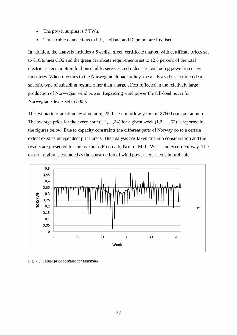
52
• The power surplus is 7 TWh.
• Three cable connections to UK, Holland and Denmark are finalised.
In addition, the analysis includes a Swedish green certificate market, with certificate prices set
to €16/tonnes CO2 and the green certificate requirements set to 12,6 percent of the total
electricity consumption for households, services and industries, excluding power intensive
industries. When it comes to the Norwegian climate policy, the analyses does not include a
specific type of subsiding regime other than a large effect reflected in the relatively large
production of Norwegian wind power. Regarding wind power the full-load hours for
Norwegian sites is set to 3000.
The estimations are done by simulating 25 different inflow years for 8760 hours per annum.
The average price for the every hour (1,2,…,24) for a given week (1,2,…, 52) is reported in
the figures below. Due to capacity constraints the different parts of Norway do to a certain
extent exist as independent price areas. The analysis has taken this into consideration and the
results are presented for the five areas Finnmark, North-, Mid-, West- and South-Norway. The
eastern region is excluded as the construction of wind power here seems improbable.
Fig. 7.5: Future price scenario for Finnmark.
0
0,05
0,1
0,15
0,2
0,25
0,3
0,35
0,4
0,45
0,5
1 11 21 31 41 51
NO
K/k
Wh
Week
nfi

53
Fig. 7.6: Future price scenario for North-Norway.
Fig. 7.7: Future price scenario for Mid-Norway.
0
0,05
0,1
0,15
0,2
0,25
0,3
0,35
0,4
1 11 21 31 41 51
NO
K/k
Wh
Week
nno
0
0,05
0,1
0,15
0,2
0,25
0,3
0,35
0,4
0,45
1 11 21 31 41 51
NO
K/k
Wh
Week
nmi

54
Fig 7.8: Future price scenario for West-Norway.
Fig. 7.9: Future price scenario for South-Norway.
For all five price regions, we see the same daily and seasonal tendencies: Higher prices during
daytime and winter and lower prices during nights and summertime. We also see a trend of
rising prices from the summer weeks towards fall. The more volatile prices for Finnmark can
be explained by grid capacity constraints. The average prices are NOK 0,33 for all regions.
Finnmark records the both the maximum and minimum prices at NOK 0,47 and NOK 0,02
respectively.
0
0,05
0,1
0,15
0,2
0,25
0,3
0,35
0,4
0,45
1 11 21 31 41 51
NO
K/k
Wh
Week
nve
0
0,05
0,1
0,15
0,2
0,25
0,3
0,35
0,4
0,45
1 11 21 31 41 51
NO
K/k
Wh
Week
nsy

55
8. Grid parity and future cost development
The purpose of this work has been to study the grid parity for wind power – the point at which
the cost of electricity from wind power will equal the cost of producing electricity by
traditional means without taking into consideration subsidies. This section compares the
levelized production costs derived in Section 6.7.2 with the average price for Norway,
Sweden, UK, the Netherlands, Denmark and Germany by the use of a Salter-diagram. In the
Salter-diagram the column width represents the production of a given wind project while the
column height represents the LPC. The average price is computed from the price data from
the scenario in Chapter 7. In the Salter-diagram grid parity is reached at the point where prices
are equal the long-run marginal cost.
8.1 Grid parity
Figure 8.1 shows the Salter-diagram based on the 12 Norwegian wind farms addressed in
Table 6.5. In order to reach its grid parity the LPC must equate the cost of conventional power
production reflected through the energy price. Inspection of Figure 8.1 shows no signs of grid
parity.
Fig. 8.1: Salter-diagram.
0
0,1
0,2
0,3
0,4
0,5
0,6
0,7
153 336 518 701 883 1066 1248 1431 1614 1797 1979 2162 2344 2527
NO
K/k
Wh
Cumulative production (GWh)
UK Netherlands Germany Denmark Norway/Sweden

56
8.2 Future cost development
Experience curve methodology describes how cost declines with cumulative production,
where cumulative production is used as an approximation for the accumulated experience in
producing and employing a technology (Neij et al., 2003). Characteristic for the experience
curves is that cost is reduced by a constant percentage with each doubling of the total number
of units produced. Generally, an experience curve is expressed as
7V r = 74 ∙ 7¡d¢
where 7V r is the cost per unit as a function of output, 74is the cost of the first unit produced, 7¡d is the cumulative production over time, and b is the experience index. For each doubling
of the cumulative production (7¡d� = 27¡d6) the relative cost reduction will be
7V r6 − 7V r�7V r6 = 1 − 2¢
where 2¢is called the progress ratio. The progress ratio is used to express the progress of cost
reduction for different technologies. For example, a progress ratio of 90 percent means that
costs are reduced with 10 percent each time the cumulative production is doubled.
In our analysis, for the best case wind farm to reach its grid parity, the LPC must decrease by
more than 32 percent. By the means of experience curve methodology this is equivalent to
progress ratio of 78 percent. As pointed out above, wind power is capital intensive. In the
capital cost function, the wind turbine constitutes of 75-80 percent of the total cost. Hence, in
order to see future cost decreases one must investigate the development in turbine costs.
Studies on experience curves for the wind turbine industry report the progress ratio to be 92
percent for Denmark and 98 percent for Germany (Neij et al., 2003). This means that costs are
expected to be reduced with between 2 and 8 percent each time the cumulative production is
doubled. Therefore, even if it was the case that the cumulative production of wind power
would double during a time span of 20 years, we should not expect the industry to reach its
grid parity. Figure 8.2 shows the Salter-diagram for an 8 decrease in the LPC-level, still as a
function of a discount rate at the 6 percentage level. Even if it was the case that the
cumulative production of wind power would double during a time span of 20 years, we should
not expect the industry to reach its grid parity.

57
Fig. 8.2: Salter-diagram for an 8 percent decrease in the LPC-level and a discount rate of 6 percent.
0
0,1
0,2
0,3
0,4
0,5
0,6
0,7
153 336 518 701 883 1066 1248 1431 1614 1797 1979 2162 2344 2527
NO
K/k
Wh
Cumulative production (GWh)
UK Netherlands Germany Denmark Norway/Sweden

58
9. Concluding remarks
During the last 20 years Europe has seen a rapid increase in the development of wind power.
During this period total generation from wind energy has increased from 0,7 TWh to more
than 100 TWH and wind power is by far the energy resource with highest relative growth rate.
The large growth is largely attributed to the growing attention to environmental problems and
security of supply. Especially, does the Stern-review (Stern, 2006) point out that a
combination of higher carbon prices and the promotion of new renewable technology is
needed in order to stabilize the emission of CO2 below 550 CO2e11. Concerns regarding the
security of supply and environmental issues were also the underlying motivation when
Norway introduced its target for the restructuring of the energy sector. Among these targets
was the production of 3 TWh from wind power by 2010.
Since the long-run marginal costs of wind power generally have exceeded the market price,
the development of wind power has been highly reluctant on subsidies. Several support
schemes have been development, but the two most common are the feed-in tariff and direct
subsidies. Norwegian wind power development has to a large extent been driven by direct
subsidies. By 2009, the Norwegian wind power industry has been subsidized with more than
NOK 1600 million, which has generated more than 1,7 TWh12.
Wind power is a capital intensive energy source. Between 70-80 percent of the total cost is
related to the upfront capital cost, whereas much as 40-70 percent of costs is related to
operation, maintenance and fuel for conventional power technology.
The purpose of this work has been to study the so-called grid parity – the point at which the
cost of electricity from wind power will equal the cost of producing electricity by traditional
means without taking into consideration subsidies. The future price has been estimated for the
five price regions along the Norwegian coast and the long-run marginal cost for 12
Norwegian wind farms has been calculated. The average price for Norway is estimated at 0,33
NOK/kWh. The long-run marginal cost for the 12 wind farms is calculated between 0,49
NOK/kWh and 0,71 NOK/kWh with a discount rate of 6 percent. Given stable costs, wind
power will not reach its grid parity.
11 See footnote 4 on CO2e. 12 700 GWh are not yet developed.

59
For the best case wind farm to reach its grid parity, following experience curve methodology,
the progress ratio must be found to be less than or equal to 78 percent. The wind power
industry is capital intensive. In the capital cost function, the wind turbine constitutes of 75-80
percent of the total. Hence, in order to see future cost decreases one must investigate the
development in turbine costs. Studies on experience curves for the wind turbine industry
report the progress ratio to be 92 percent for Demark and 98 percent for Germany. This means
that costs are reduced with between 2 and 8 percent each time we the cumulative production
is doubled. Again, we cannot conclude that Norwegian wind power will reach its grid parity
within the next 15-20 years.
When compared to early feed-in schemes used in Germany from 1990 to 1997, the Norwegian
subsidy regime established in 2000 seems to generate more wind power in terms of GWh
during the 7 consecutive years (see Section 4.2). This thesis does not provide a thorough
analysis on the topic, it has not even been the scope of the thesis. However, as the use of
direct subsidies for the benefit of Norwegian wind power development continues, more data
will be available and these indications should be subject for further research.
60
References
Berge, E., Nyhammer, F., Tallhaug, L., Villanger, F, Bremnes, J.B., Køltzow, M.Ø., Smits, J.,
Knauer, A, 2002. Forecasting wind and wind energy production in Norwegian wind farms.
www.vindteknikk.no/filesystem/2006/12/forecast_wind_energy_16.pdf
Bryars, S., Holt, J., 2008. European wind farm project cost. Garrad Hassan report for Enova
SF.
Bye, T., Halvorsen, B., 1998. Økonomiske målsettinger og resultater av energiloven.
Økonomiske rapporter 8/98, Statistisk sentralbyrå.
Bye, T., Hope, E., 2005. Deregulation of electricity – The Norwegian experience. Discussion
papers No. 433, Statistics Norway.
Bye, T., Strøm, S., 2008. Norsk kraft i hundre år – utvikling og økonomisk teori.
Samfunnsøkonomen nr. 6.
ECON, 1998. Vindkraft i Norge.
Flagstad, K., Gakkestad, K., Gundersen, M.H., Hofstad, K., Jensen, T., Jensen, T., Kolseth,
K., Selfors, A., 2004. Grønne sertifikater. NVE Rapport nr 11.
Hofstad, K., 2009. Vindkraft – produksjonsstatistikk. NVE.
IEA, 2008. World Energy Outlook.
Krohn, S., Morthorst, P.E, Awerbuch, S., 2009. The Economics of wind energy. A report by
the European Wind Energy Association.
Menanteau, P., Finon, D., Lamy, M., 2003. Prices versus quantities: choosing policies for
promoting the development of renewable energy. Energy Policy 31, 799-812.
Morthorst, P.E., 1999a. Capacity development and profitability of wind turbines. Energy
Policy 27, 779-787.
Morthorst, P.E., 1999b. Danish renewable energy and a green certificate market. In: Design of
Energy Markets and Environment, Conference Papers, Copenhagen, 20-21 May 1999, Nordic
Energy Research Program.

61
Morthorst, P.E., 2000. The development of a green certificate market. Energy Policy 28,
1085-1094.
Morthorst, P.E., Jensen, S.G., Meibom, P., 2005. Investering og prisdannelse på et liberalisert
elmarked. Forskningscenter Risø.
Neij, L., Andersen, P.D., Durstewitz, M., Helby, P., Hoppe-Kilpper, M., Morthorst, P.E.,
2003. Experience curves: A tool for energy policy assessment. Environmental and Energy
Systems Studies.
Ragwitz, M., Huber C., 2005. Feed-in systems in Germany and Spain and a comparison.
Fraunhofer Institut für Systemtechnik und Innovationsforschung.
Statnett, 2008. Nettutviklingsplan for sentralnettet 2008-2025.
Statnett, 2009. Sentralnettstariffen 2009.
Stein, J.C., 1989. Efficient Capital Markets, Inefficient Firms: A Model of Myopic Corporate
Behavior. The Quarterly Journal of Economics, Vol. 104, No. 4, 655-669.
Stern, N., 2006. The Economics of climate change: The Stern review. Cambridge University
Press.
Tande, J.O., Hunter, R., 1994. Estimation of cost of energy from wind energy conversion
systems 2nd edition. IEA.
Varian, H., 1992. Microeconomic analysis 3rd edition. W. W. Norton & Company, Inc.

62
Appendix A
Fig. A.1: Future prices UK.
Fig. A.2: Future prices the Netherlands.
0
0,2
0,4
0,6
0,8
1
1,2
1,4
1,6
1,8
1 11 21 31 41 51
NO
K/k
Wh
Week
UK
0
0,2
0,4
0,6
0,8
1
1,2
1,4
1 11 21 31 41 51
NO
K/k
Wh
Week
nl

63
Fig.: A.3: Future prices North-Germany.
Fig. A.4: Future prices Denmark.
0
0,2
0,4
0,6
0,8
1
1,2
1,4
1 11 21 31 41 51
NO
K/k
Wh
Week
de_n
0
0,1
0,2
0,3
0,4
0,5
0,6
0,7
0,8
1 11 21 31 41 51
NO
K/k
Wh
Week
jut

64
Fig.: A.5: Future prices Sweden region 1.
Fig. A.6: Future prices scenario Sweden region 2.
0
0,05
0,1
0,15
0,2
0,25
0,3
0,35
0,4
0,45
1 11 21 31 41 51
NO
K/k
Wh
Week
se1
0
0,05
0,1
0,15
0,2
0,25
0,3
0,35
0,4
0,45
1 11 21 31 41 51
NO
K/k
Wh
Week
se2

65
Fig. A.7: Future price scenario Sweden region 3.
Fig. A.8: Future price scenario Sweden region 4.
0
0,05
0,1
0,15
0,2
0,25
0,3
0,35
0,4
0,45
0,5
1 11 21 31 41 51
NO
K/k
Wh
Week
se3
0
0,1
0,2
0,3
0,4
0,5
0,6
1 11 21 31 41 51
NO
K/k
Wh
Week
se4

66