Embed Size (px)
Citation preview

Paths and pitfalls in prediction verification
Thordis L. ThorarinsdottirNorwegian Computing Center
Tilmann Gneiting, Sebastian Lerch and Nadine GissiblHeidelberg University, Germany
Norges Bank, January 14 2013
1 / 27

Prediction evaluation for real valued events fallsin three classes
(a) Forecast
0 2 4 6 8 10
(b) Observation
0 2 4 6 8 10
(c) Comparison
0 2 4 6 8 10
0 2 4 6 8 10 0 2 4 6 8 10 0 2 4 6 8 10
0 2 4 6 8 10 0 2 4 6 8 10 0 2 4 6 8 10
2 / 27

Forecasts ought to be probabilistic in nature
All those whose duty it is to issue regular daily forecasts know thatthere are times when they feel very confident and other times whenthey are doubtful as to coming weather. It seems to me that thecondition of confidence or otherwise forms a very important part ofthe prediction.
Cooke (1906)
However,I some applications require a deterministic predictionI the full predictive distribution might not be available
Gneiting, T. (2011): Making and evaluating point forecasts.JASA, 106, 746-762.
3 / 27

Part I: Verification of extreme events
4 / 27

Probabilistic forecasts should be evaluated usingproper scoring rules
Definition (Murphy and Winkler, 1968)
If F denotes a class of probabilistic forecasts on R, a properscoring rule is any function
R : F × R→ R
such that
R(G ,G ) := EG R(G ,Y ) ≤ EG R(F ,Y ) =: R(F ,G )
for all F ,G ∈ F .
5 / 27

The class of proper scoring rules is large
Squared Error (SE) R(F , y) = (mean(F )− y)2
Logarithmic Score (IS) R(F , y) = − log(f (y))
Continuous Ranked R(F , y) =∫
[F (x)− 1{x ≥ y}]2dxProbability Score (CRPS) = EF |X − y | − 1
2EFEF |X − X ′|
Gneiting, T. and Raftery, A.E. (2007): Strictly proper scoringrules, prediction and estimation. JASA, 102, 359-378.
6 / 27

Do you know the proper scoring rule?Three scoring rules as a function of the observed value for GEVswith location 0, scale 1, and varying shape parameter.
y
Score
−4 −2 0 2 4
01
23
4 (a)
yScore
−4 −2 0 2 40
12
34 (b)
y
Score
−4 −2 0 2 4
01
23
4 (c)
y
Score
0 1 2 3 4 5
01
23
4 (d)
y
Score
0 1 2 3 4 5
01
23
4 (e)
y
Score
0 1 2 3 4 5
01
23
4 (f)
Figure 1: The CRPS (solid lines), the ignorance score (dashed lines), and the quantile score for τ = 0.5(dotted lines) as a function of the observation value for the GEV (top row) and the GPD (bottom row). Thepredictive distributions have zero location (µ = 0), standard scale (σ = 1), and shape ξ = −0.5 (firstcolumn), ξ = 0 (second column), or ξ = 0.5 (third column). The corresponding predictive densities areindicated in gray.
39
The candidates are
(a) R(F , y) = 0.5|median(F )− y |
(b) R(F , y) = EF |X − y | − 12EFEF |X − X ′|
(c) R(F , y) = − log(f (y))
7 / 27

Media attention often falls on predictionperformance in the case of extreme events
How did economists get it so wrong? NY Times, 2009
Nouriel Roubini: The economist who predicted Guardian, 2009worldwide recession
An exclusive interview with Med Yones – the CEOQ Mag, 2010expert who predicted the financial crisis
Bill Giles accepts blame for BBC Great Storm failures Daily Tel, 2011
Bad data failed to predict Nashville Flood NBC, 2011
8 / 27

Verifying only the extremes erases propriety
Amisano and Giacomini (JBES, 2007) consider the restricted score
R∗(F , y) = −1{y ≥ t} log f (y)
However, if g(y) > f (y) for all y ≥ t, then
ER∗(G , y) < ER∗(F , y)
independent of the true sampling density.
Indeed, if the forecaster’s belief is F , his best prediction under R∗ is
g(y) = f (y)∫∞t f (x)dx1{y ≥ t}
(Gneiting and Ranjan, JBES, 2011).
9 / 27

Demonstration by simulation
True data distribution: Gt = N(µt , 1) with µt ∼ N(0, 1).
(a)
PIT
Rel
ativ
e Fr
eque
ncy
0.0 0.2 0.4 0.6 0.8 1.0
0.0
0.5
1.0
1.5
2.0
2.5
3.0
(b)
PIT
Rel
ativ
e Fr
eque
ncy
0.0 0.2 0.4 0.6 0.8 1.0
0.0
0.5
1.0
1.5
2.0
2.5
3.0
(c)
PIT
Rel
ativ
e Fr
eque
ncy
0.0 0.2 0.4 0.6 0.8 1.0
0.0
0.5
1.0
1.5
2.0
2.5
3.0
(d)
PITR
elat
ive
Freq
uenc
y
0.0 0.2 0.4 0.6 0.8 1.0
0.0
0.5
1.0
1.5
2.0
2.5
3.0
(e)
PIT
Rel
ativ
e Fr
eque
ncy
0.0 0.2 0.4 0.6 0.8 1.0
0.0
0.5
1.0
1.5
2.0
2.5
3.0
Figure 3.1.: PIT histograms for (a) the ideal forecaster, (b) the climatologicalforecaster, (c) the unfocused forecaster, (d) the sign-biased forecasterand (e) the biased forecaster for 10 000 repetitions of the predictionexperiment.
−4 −2 0 2 4 6
0.0
0.1
0.2
0.3
0.4
x
Density
idealclimatologicalunfocusedsign−biasedbiased
Figure 3.2.: Marginal predictive densities of the forecasters given in Table 3.1.
33
Forecaster Ft
Ideal N(µt , 1)Sign-biased N(−µ1, 1)Climatological N(0, 2)Unfocused 1
2{N(µt , 1)+N(µt + τt , 1)}
Biased N(µt + 2.5, 1)
Here, τt = ±1 with probability 1/2.
10 / 27
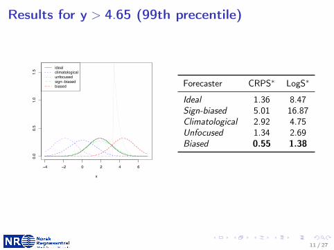
Results for y > 4.65 (99th precentile)
−4 −2 0 2 4 6
0.0
0.5
1.0
1.5
x
Con
ditio
nal d
ensi
ty
idealclimatologicalunfocusedsign−biasedbiased
Figure 3.4.: Marginal predictive densities of the forecasters given in Table 3.1 giventhat the observation is larger than the 99th percentile of the marginaldistribution, for which the corresponding conditional density is indi-cated by the dotted black line.
Table 3.3.: Average values of the CRPS, the LogS, the mean absolute error (MAE)and the empirical coverage (in %) of 80% prediction intervals for thesubset of observations larger than the 99th percentile of the marginaldistribution of the observations.
Forecaster CRPS LogS MAE Coverage
Ideal 1.36 8.47 1.86 18.1Climatological 2.92 4.75 3.72 0.0Unfocused 1.34 2.69 1.84 30.0Sign-biased 5.01 16.87 5.58 0.0Biased 0.55 1.38 0.79 81.9
36
Forecaster CRPS∗ LogS∗
Ideal 1.36 8.47Sign-biased 5.01 16.87Climatological 2.92 4.75Unfocused 1.34 2.69Biased 0.55 1.38
11 / 27

Same holds for all restrictions y > t with t > 20.0 0.2 0.4 0.6 0.8 1.0
01
23
4Threshold (quantile)
Res
trict
ed C
RPS
idealclimatologicalunfocusedsignbiasedbiased
−3 −2 −1 0 1 2 3
01
23
4
Threshold (value)
Res
trict
ed C
RPS
idealclimatologicalunfocusedsignbiasedbiased
0.0 0.2 0.4 0.6 0.8 1.0
02
46
810
Threshold (quantile)
Res
trict
ed L
ogS
idealclimatologicalunfocusedsignbiasedbiased
−4 −2 0 20
24
68
10Threshold (value)
Res
trict
ed L
ogS
idealclimatologicalunfocusedsignbiasedbiased
0.0 0.2 0.4 0.6 0.8 1.0
01
23
45
Threshold (quantile)
MAE
idealclimatologicalunfocusedsign−biasedbiased
−4 −2 0 2
01
23
45
Threshold (value)
MAE
idealclimatologicalunfocusedsign−biasedbiased
0.0 0.2 0.4 0.6 0.8 1.0
0.0
0.2
0.4
0.6
0.8
1.0
Threshold (quantile)
Cov
erag
e
idealclimatologicalunfocusedsign−biasedbiased
−4 −2 0 2
0.0
0.2
0.4
0.6
0.8
1.0
Threshold (value)
Cov
erag
e
idealclimatologicalunfocusedsign−biasedbiased
Figure 3.5.: Summary measures for subsets of extreme values as functions of thethreshold defining extreme values in terms of quantiles of the marginaldistribution (left column) or values (right column).
37
12 / 27

The results are highly significant
0.0 0.2 0.4 0.6 0.8 1.0
−80
−60
−40
−20
0
(a)
Threshold (quantile)
t n
0.0 0.2 0.4 0.6 0.8 1.0
−300
−200
−100
−50
0
(b)
Threshold (quantile)
t n
0.0 0.2 0.4 0.6 0.8 1.0
0.0
0.2
0.4
0.6
0.8
1.0
Threshold (quantile)
p−va
lue
0.0 0.2 0.4 0.6 0.8 1.0
0.0
0.2
0.4
0.6
0.8
1.0
Threshold (quantile)
p−va
lue
Figure 3.6.: Top row: Diebold-Mariano-type test statistic (3.1) for test of equalperformance comparing the ideal and the biased forecaster as functionsof the threshold which defines extreme events, using (a) the restrictedCRPS and (b) the restricted LogS. Bottom row: Corresponding p-values under the standard normal hypothesis, the dashed lines indicatea 5% significance level.
For both restricted CRPS and restricted LogS, the Diebold-Mariano-type teststatistics for the comparison of the ideal and the biased forecaster shown in Fig-ure 3.6 are negative up to a threshold value of approximately the 90th percentileof the marginal distribution of the observations, which corresponds to a value ofaround 2, and positive for larger threshold values. The measured score differencesare significant, except for a small interval of thresholds around the 90th percentileof the marginal distribution as indicated by the corresponding p-value plots. Inparticular, the tests of equal performance prefer the biased forecaster over theideal forecaster for extreme events and the measured score differences are signifi-cant even for small significance levels. This observation again confirms our findingof the impropriety of the restricted CRPS and the restricted LogS.
3.3.3. Proper scoring rules for extreme events
Gneiting and Ranjan (2011b) and Diks et al. (2011) propose proper scoring rulesfor extreme events which were discussed in 2.3.2. We apply the threshold-weighted
39
Diebold-Mariano tests for equal performance of the ideal and the biasedforecaster under (a) CRPS∗ and (b) LogS∗.
13 / 27

Better: Use threshold-weighted scoring rulesDiks et al. (JE, 2011) propose the conditional likelihood score
R(F , y) = −ω(y) log( f (y)∫
ω(x)f (x)dx
)
and the cencored likelihood score
R(F , y) = −[ω(y) log f (y) + (1− ω(y)) log
(1−
∫ω(x)f (x)dx
)].
Gneiting and Ranjan (JBES, 2011) propose the thresholdweighted CRPS
R(F , y) =
∫(F (x)− 1{y ≤ x})2ω(x)dx .
Here, we may e.g. set ω(x) = 1{x ≥ r}.14 / 27

Ideal forecaster is now the preferred forecaster
0.0 0.2 0.4 0.6 0.8 1.0
−80
−60
−40
−20
0
(a)
Threshold (quantile)
t n
0.0 0.2 0.4 0.6 0.8 1.0
−80
−60
−40
−20
0
(b)
Threshold (quantile)
t n0.0 0.2 0.4 0.6 0.8 1.0
−80
−60
−40
−20
0
(c)
Threshold (quantile)
t n
0.0 0.2 0.4 0.6 0.8 1.0
−80
−60
−40
−20
0
(d)
Threshold (quantile)
t n
0.0 0.2 0.4 0.6 0.8 1.0
0.0
0.1
0.2
0.3
0.4
0.5
Threshold (quantile)
p−va
lue
0.0 0.2 0.4 0.6 0.8 1.0
0.0
0.1
0.2
0.3
0.4
0.5
Threshold (quantile)
p−va
lue
0.0 0.2 0.4 0.6 0.8 1.0
0.0
0.1
0.2
0.3
0.4
0.5
Threshold (quantile)
p−va
lue
0.0 0.2 0.4 0.6 0.8 1.0
0.0
0.1
0.2
0.3
0.4
0.5
Threshold (quantile)
p−va
lue
Figure 3.7.: Diebold-Mariano-type test statistics (3.1) for tests of equal perfor-mance using the threshold-weighted CRPS to compare the ideal fore-caster with (a) the climatological, (b) the unfocused, (c) the sign-biased and (d) the biased forecaster as functions of the threshold r in(3.2). The second row shows corresponding p-values under the stan-dard normal hypothesis, with dashed lines indicating a 5% significancelevel.
continuous ranked probability score,
CRPSt(f, y) =
� ∞
−∞(F (z) − {y ≤ z})2w(z)dz,
the conditional likelihood scoring rule,
CL(f, y) = −w(y) log
�f(y)�
w(s)f(s)ds
�,
and the censored likelihood scoring rule,
CSL(f, y) = −�w(y) log f(y) + (1 − w(y)) log
�1 −
�w(s)f(s)ds
��,
to the competing forecasting procedures and study effects of sample size, varianceestimation and the choice of weight functions. At first, we will assume the weightfunction w to be an indicator function,
wr(x) = (x ≥ r), (3.2)
where r ∈ R is a real-valued threshold. Later, we will study different weightfunctions.
Figure 3.7 shows plots of the test statistic tn as a function of r, in terms of
40
Diebold-Mariano tests for comparing the ideal forecaster with (a) theclimatological, (b) the unfocused, (c) the sign-biased, and (d) the biasedforecaster under the threshold-weighted CRPS.
15 / 27

The conditional likelihood score seems less robust
0.0 0.2 0.4 0.6 0.8 1.0
−250
−150
−50
0
(a)
Threshold (quantile)
t n
0.0 0.2 0.4 0.6 0.8 1.0
−250
−150
−50
0
(b)
Threshold (quantile)
t n0.0 0.2 0.4 0.6 0.8 1.0
−250
−150
−50
0
(c)
Threshold (quantile)
t n
0.0 0.2 0.4 0.6 0.8 1.0
−250
−150
−50
0
(d)
Threshold (quantile)
t n
0.0 0.2 0.4 0.6 0.8 1.0
0.0
0.2
0.4
0.6
0.8
1.0
Threshold (quantile)
p−va
lue
0.0 0.2 0.4 0.6 0.8 1.0
0.0
0.2
0.4
0.6
0.8
1.0
Threshold (quantile)
p−va
lue
0.0 0.2 0.4 0.6 0.8 1.0
0.0
0.2
0.4
0.6
0.8
1.0
Threshold (quantile)
p−va
lue
0.0 0.2 0.4 0.6 0.8 1.0
0.0
0.2
0.4
0.6
0.8
1.0
Threshold (quantile)
p−va
lue
Figure 3.8.: Diebold-Mariano-type test statistics (3.1) for tests of equal perfor-mance using the conditional likelihood scoring rule to compare theideal forecaster with (a) the climatological, (b) the unfocused, (c) thesign-biased and (d) the biased forecaster as functions of the thresh-old r in (3.2). The second row shows corresponding p-values underthe standard normal hypothesis, with dashed lines indicating a 5%significance level.
quantiles of the marginal distribution of the observations, for the comparison ofthe ideal forecaster and the competing forecasting procedures using the threshold-weighted CRPS. In case of negative values of the test statistic the ideal forecasteris preferred over the competitor, for positive values the competitor is preferredover the ideal forecaster. The asymptotic variance of the score difference wasestimated as proposed by Gneiting and Ranjan (2011b). We will investigate theeffects of different variance estimation procedures below. In all four cases, theideal forecaster is preferred over his competitor for all choices of r, all observedscore differences are significant under the standard normal hypothesis. Note thathere, the sample size equals T for any choice of r, which was not the case for therestricted scoring rules used in the previous section. Thus, the standard normalhypothesis is much more likely to hold in the case of larger values of r as well.
Figures 3.8 and 3.9 show analogous plots for the conditional and the censoredlikelihood scoring rule. Here, the asymptotic variance of the score differences wasestimated as proposed by Diks et al. (2011). For the conditional likelihood scoringrule, all observed values of the test statistics are negative, however, the observeddifferences are much less significant under the standard normal hypothesis. Thescore differences between the ideal and the unfocused forecaster are only signif-icant up to approximately r = 0.5 which corresponds to the 60th percentile ofthe marginal distribution of the observations. The conditional likelihood scor-ing rule is furthermore unable to significantly distinguish between the predictiveperformance of the ideal and the biased forecaster for thresholds larger than the
41
Diebold-Mariano tests for comparing the ideal forecaster with (a) theclimatological, (b) the unfocused, (c) the sign-biased, and (d) the biasedforecaster under the conditional likelihood score.
16 / 27

The results depend heavily on the varianceestimation in the Diebold-Mariano test
0.0 0.2 0.4 0.6 0.8 1.0
−150
−100
−50
050
(a)
Threshold (quantile)
t n
GRDPvD
0.0 0.2 0.4 0.6 0.8 1.0
−200
−100
0
(b)
Threshold (quantile)t n
GRDPvD
0.0 0.2 0.4 0.6 0.8 1.0
−300
−200
−100
010
0
(c)
Threshold (quantile)
t n
GRDPvD
0.0 0.2 0.4 0.6 0.8 1.0
0.0
0.2
0.4
0.6
0.8
1.0
Threshold (quantile)
p−va
lue
GRDPvD
0.0 0.2 0.4 0.6 0.8 1.0
0.0
0.2
0.4
0.6
0.8
1.0
Threshold (quantile)
p−va
lue
GRDPvD
0.0 0.2 0.4 0.6 0.8 1.0
0.0
0.2
0.4
0.6
0.8
1.0
Threshold (quantile)
p−va
lue
GRDPvD
Figure 3.13.: Test statistics tn for tests of equal performance using (a) thethreshold-weighted CRPS, (b) CL and (c) CSL scoring rule to com-pare the ideal and the biased forecaster as functions of the thresholdr. The asymptotic variance was estimated as proposed by Gneitingand Ranjan (2011b) (GR, blue) and Diks et al. (2011) (DPvD, red).The bottom row shows the corresponding p-values under the stan-dard normal hypothesis. Note that for clarity of the presentation,the scale of the test statistics varies in the plots in the top row.
cedure proposed by Gneiting and Ranjan (2011b). For both the threshold-weightedCRPS and the CL scoring rule, the observed score differences are not significantfor thresholds larger than approximately the 70th percentile of the marginal dis-tribution of the observations if the HAC estimator of Diks et al. (2011) is used.Neither are the censored likelihood score differences for thresholds larger than thecorresponding 95th percentile. As opposed to this, the score differences for all scor-ing rules are significant for all thresholds if the variance is estimated as proposedby Gneiting and Ranjan (2011b), except for the CL scoring rule and very largethresholds.
The estimator of the asymptotic variance proposed by Gneiting and Ranjan(2011b) is based on the theoretical assumption of Diebold and Mariano (1995)that optimal k-step-forecast errors are at most (k − 1)-dependent. However, thisassumption of (k − 1)-dependence might be violated in practice due to variousreasons. In our simulation study, the values of the scoring rules, which can be in-terpreted as forecast errors, are 0-dependent by construction. This can empiricallybe confirmed by computing estimates of the autocorrelation, as shown in Fig-ure 3.15 for the ideal forecaster. Qualitatively equivalent results can be obtainedfor all other forecasting procedures. Thus, the approach to variance estimationused by Gneiting and Ranjan (2011b) seems to be a reasonable choice for our sim-ulation study, while the approach proposed by Diks et al. (2011) takes into accountunnecessary large amounts of autocorrelation up to lag 10.
46
Diebold-Mariano tests for comparing the ideal and the biased forecasterunder(a) the threshold weighted CRPS, (b) the conditional likelihoodscore, and (c) the cencored likelihood score.
17 / 27

Part II: Verification of distributions of events
18 / 27

Propriety condition for divergences
Two distributions may be compared using a divergence function,
d : F × F → [0,∞], d(F ,F ) = 0 ∀F ∈ F .
Definition (T, Gneiting and Gissibl, 2013)
Let Y1, . . . ,Yk ∼ G and Gk(x) = 1k∑k
i=1 1{x ≥ Yi} be thecorresponding empirical CDF. A divergence function d is n-proper if
E d(G ,Gk) ≤ E d(F ,Gk)
for k = 1, . . . , n and all F ,G ∈ F . Similarly, d is asymptoticallyproper if
limk→∞
E d(G ,Gk) ≤ limk→∞
E d(F ,Gk),
for all F ,G ∈ F .
19 / 27

Examples of proper score divergences
Squared Mean Value d(F ,G ) = [mean(F )−mean(G )]2 SE
Integrated Quadratic d(F ,G ) =∫
[F (x)− G (x)]2dx CRPS
Kullback-Leibler d(F ,G ) =∫g(y) log g(y)
f (y)dλ(y) LogS
Dawid-Sebastiani d(F ,G ) = tr(Σ−1F ΣG )− log det(Σ−1
F ΣG ) DS
+(µF − µG )′Σ−1F (µF − µG )−m
20 / 27

Every proper scoring rule defines an n-properdivergence function
Theorem (T,Gneiting and Gissibl, 2013)
Assume that R(G ,G ) 6= +∞ and let
d(F ,G ) = R(F ,G )− R(G ,G ),
where R is a proper scoring rule. Then d is n-proper for alln = 1, 2, . . ..
Note thatI d(Fm,Gk) and 1
k∑k
i R(Fm, yi ) will result in the same rankingof F1, . . . ,FM .
I it holds that d(G ,G ) = 0, while R(G ,G ) might depend on G .
21 / 27

Example: How skillful are climate models?Introduction
Global temperature data (1980, from GHCN)
−20
−15
−10
−5
0
5
10
15
20
25
30
Finn Lindgren - [email protected] Toledo Spring School: GMRF, SPDE, INLA (1+2+3a) 4/60
Average yearly temperature in 1980, figure by Finn Lindgren.
22 / 27

Prediction framework
0
2
4
6
8
IQ divergence forECHAM5/MPI-OM vs. NCEP-1
We considerI 15 climate models and 2
re-analysesI 154 grid points over EuropeI Yearly maximum
temperatures 1961-1990
23 / 27

Main goal: Detection of poor skill0
12
34
56
IQ d
ista
nce
NC
EP
−1/
ER
A−
40
CG
CM
3.1(
T47
)
CG
CM
3.1(
T63
)
CN
RM
−C
M3
CS
IRO
−M
k3.0
CS
IRO
−M
k3.5
EC
HA
M5/
MP
I−O
M
FG
OA
LS−
g1.0
GF
DL−
CM
2.0
GF
DL−
CM
2.1
GIS
S−
AO
M
GIS
S−
EH
GIS
S−
ER
MIR
OC
3.2(
hire
s)
MIR
OC
3.2(
med
res)
MR
I−C
GC
M2.
3.2
010
2030
4050
6070
MV
div
erge
nce
NC
EP
−1/
ER
A−
40
CG
CM
3.1(
T47
)
CG
CM
3.1(
T63
)
CN
RM
−C
M3
CS
IRO
−M
k3.0
CS
IRO
−M
k3.5
EC
HA
M5/
MP
I−O
M
FG
OA
LS−
g1.0
GF
DL−
CM
2.0
GF
DL−
CM
2.1
GIS
S−
AO
M
GIS
S−
EH
GIS
S−
ER
MIR
OC
3.2(
hire
s)
MIR
OC
3.2(
med
res)
MR
I−C
GC
M2.
3.2
Average over all grid points compared to ERA40 (blue) and NCEP-1 (red)
24 / 27

Many common divergences are not n-proper
The area validation metric is given by
d(F ,G ) =∫|F (x)− G (x)|dx
k
1 5 10 15 20 25
0.0
0.1
0.2
0.3
Observations: U([0, 1]) (solid line)Forecasts: discrete with mass 1
k+1 in i/k for i = 1, . . . , k (dashed line)
25 / 27

Many common divergences are not n-proper
The Smirnov distance is given by
d(F ,G ) = supx |F (x)− G (x)|
k
1 2 3 4 5 6 7 8 9 10
0.25
0.50
0.75
Observations: U([0, 1]) (solid line)Forecasts: discrete with mass 1
k+1 in i/k for i = 0, . . . , k (dashed line)
26 / 27

Conclusions
I The verification measure may influence the results of acomparative study and should thus be selected with care.Proper scores/divergences for probabilistic predictions preventhedging strategies.
I It may be useful to use more than one method to verify aprobabilistic prediction method, as different scores/divergencesmay focus on different parts of the distribution.
I One must be careful when “handpicking” certain events for theverification.
27 / 27