NORTHWESTERN UNIVERSITY

Five Projects in Pattern Formation, Fluid Dynamics and Computational

Neuroscience

A DISSERTATION

SUBMITTED TO THE GRADUATE SCHOOLIN PARTIAL FULFILLMENT OF THE REQUIREMENTS

for the degree

DOCTOR OF PHILOSOPHY

Field of Applied Mathematics

By

Alexander C. Roxin

EVANSTON, ILLINOIS

December 2003

ABSTRACT

Five Projects in Pattern Formation, Fluid Dynamics and Computational

Neuroscience

Alexander Roxin

This dissertation is a compilation of five projects, which span the fields of pattern

formation, fluid dynamics and computational neuroscience. The first two chapters

deal with spatio-temporal patterns that may arise in various spatially extended sys-

tems driven far from equilibrium. In the first, the interaction of dispersionless travel-

ing waves with a long-wave mode is studied, revealing two distinct instabilities, one

of the phase and the other of the amplitude of the traveling waves. The amplitude-

driven instability can lead to localized pulses in some cases. In the second the effect

of anisotropy in rotating convection is investigated using a phenomenological Swift-

Hohenberg equation. Stability results from an amplitude-equation approach are used

to explain spirals and targets seen in experiment.

In the third chapter the question of fluid slip at a solid interface is addressed

at a molecular scale using methods from solid-state physics and nonlinear dynamics

theory. We propose a modification of the well-known Frenkel-Kontorova model based

on results from molecular dynamics simulations. The resulting dynamics explain the

phenomenon of slip as the motion of defects in the fluid layer adjacent to the solid.

The fourth and fifth chapters enter the realm of computational neuroscience. The

fourth chapter discusses how CA1 pyramidal neurons in the hippocampus actively

integrate their two principal excitatory inputs. Extensive numerical simulations using

NEURON with realistic morphological data reveals that dendritic sodium spikes may

ii

forward-propagate to the soma causing a somatic action potential if the inputs are

sufficiently synchronous. The final chapter introduces a model of excitable integrate-

and-fire neurons in a small-world network, a network with regular, local coupling

and a number randomly placed, long-range connections. The ensemble average of

the network dynamics exhibits a transition from persistent activity to failure as a

function of the density of global connections. Patterns of activity can be periodic or

chaotic depeding on parameters and the network is bistable in the persistent regime.

iii

ACKNOWLEDGEMENTS

First and foremost I thank my thesis advisor Hermann Riecke for his patience and

guidance. My collaboration with him has taught me much, not only about how to

conduct research, but about the role of a researcher more broadly.

I thank all those people with whom I’ve had the pleasure of working: Bill Kath,

Seth Lichter, Shreyas Mandre, Hermann Riecke, Sara Solla, and Nelson Spruston. I

also thank the Spruston lab for their hospitality and for humoring me.

I appreciatively acknowledge the support and funding of the NSF-IGERT grant

“Dynamics of Complex Systems in Science and Engineering” and those faculty mem-

bers who run the program day to day. Thanks also to Judy Piehl and Edla D’Herckens

for all of their help during my stay in the Department of Engineering Sciences and

Applied Mathematics.

I would also like to acknowledge the following grants: Engineering Research Pro-

gram of the Office of Basic Energy Sciences at the Department of Energy (DE-FG02-

92ER14303), NSF (DMS-9804673), NSF-IGERT fellowship through grant DGE-9987577.

Finally, I reserve my deepest gratitude to my girlfriend Libertad who taught me

that putting in a full day at work is not the same as leading a full life.

iv

Contents

List of figures . . . . . . . . . . . . . . . . . . . . . . . . . . . . . . . . . . vi

1 Introduction 1

2 Traveling Waves in an Advected Field 4

2.1 Overview of Small-Amplitude Waves in Fields . . . . . . . . . . . . . 4

2.2 The Extended Ginzburg-Landau Equations . . . . . . . . . . . . . . . 7

2.3 Phase Instability . . . . . . . . . . . . . . . . . . . . . . . . . . . . . 16

2.4 Amplitude Instability: Modulated Waves . . . . . . . . . . . . . . . . 24

2.5 Conclusion . . . . . . . . . . . . . . . . . . . . . . . . . . . . . . . . . 31

3 Modulated Rotating Convection 34

3.1 Overview of Rotating Convection . . . . . . . . . . . . . . . . . . . . 34

3.2 The stability of rolls with anisotropy . . . . . . . . . . . . . . . . . . 36

3.3 Modulated rotating convection: spirals and targets . . . . . . . . . . 40

3.4 Conclusion . . . . . . . . . . . . . . . . . . . . . . . . . . . . . . . . . 43

4 Slip at a Liquid-Solid Interface 47

4.1 Evidence of slip . . . . . . . . . . . . . . . . . . . . . . . . . . . . . . 47

v

4.2 The Frenkel-Kontorova Equation . . . . . . . . . . . . . . . . . . . . 49

4.3 Slip dynamics in the FK model . . . . . . . . . . . . . . . . . . . . . 54

4.4 Commensurate chains with integer values of ξ . . . . . . . . . . . . . 59

4.5 Commensurate chains with ξ near an integer value . . . . . . . . . . . 62

4.6 Non-integer values of ξ . . . . . . . . . . . . . . . . . . . . . . . . . . 69

4.7 The FK model and Liquid Slip . . . . . . . . . . . . . . . . . . . . . 73

4.8 Molecular Dynamics Simulations . . . . . . . . . . . . . . . . . . . . 75

4.9 The variable-density Frenkel-Kontorova Model . . . . . . . . . . . . . 85

4.10 Conclusion . . . . . . . . . . . . . . . . . . . . . . . . . . . . . . . . . 97

5 A Novel Interaction of Shaeffer Collateral and Temporo-Ammonic

Inputs in a Model of a CA1 Pyramidal Cell 98

5.1 The SC and TA pathways . . . . . . . . . . . . . . . . . . . . . . . . 98

5.2 A model of a CA1 Pyramidal cell in NEURON . . . . . . . . . . . . . 101

5.3 Response to single inputs . . . . . . . . . . . . . . . . . . . . . . . . . 110

5.4 Paired SC and TA inputs . . . . . . . . . . . . . . . . . . . . . . . . . 120

5.5 Conclusion . . . . . . . . . . . . . . . . . . . . . . . . . . . . . . . . . 132

6 Excitable Integrate-and-Fire Neurons in a Small-World Network 134

6.1 Integrate-and-Fire neurons in networks . . . . . . . . . . . . . . . . . 134

6.2 Transition from Persistent Activity to Failure . . . . . . . . . . . . . 139

6.3 Activity for slow waves. . . . . . . . . . . . . . . . . . . . . . . . . . 146

6.4 Bistability and Noise . . . . . . . . . . . . . . . . . . . . . . . . . . . 164

6.5 Conclusion . . . . . . . . . . . . . . . . . . . . . . . . . . . . . . . . . 170

vi

A Derivation of amplitude equations 174

B Derivation of Peierls-Nabarro potential 183

C Probabilities for defect generation 187

vii

List of Figures

2.1 Eigenvalues and stability balloons for traveling waves . . . . . . . . . 142.2 Transition in stabibility balloon from Eckhaus to finite wavenumber. . 162.3 Dependence of stability curve on group velocity. Dependence of most

unstable wavenumber on damping of C-field. . . . . . . . . . . . . . . 212.4 Space-time diagram of Eckhaus-like instability. . . . . . . . . . . . . . 232.5 Egienvalues and linear stability balloon for modulated traveling waves. 252.6 Bifurcation diagram of modulated traveling waves. . . . . . . . . . . . 282.7 Space-time diagram of modulated traveling waves. . . . . . . . . . . . 292.8 Bifurcation diagram of subcritical travling waves. . . . . . . . . . . . 302.9 Bifurcation diagram of localized traveling pulses. . . . . . . . . . . . . 32

3.1 Linear stability balloon for rolls in rotating convection with weak anisotropy 383.2 Example of roll stabilization through anisotropy. . . . . . . . . . . . . 393.3 Spiral and target patterns in a Swift-Hohenberg model of rotating con-

vection with anisotropy. . . . . . . . . . . . . . . . . . . . . . . . . . 413.4 Stable spiral patterns with chaotic core in a Swift-Hohenberg model. . 45

4.1 Ground state of unforced ξ = 23

chain. . . . . . . . . . . . . . . . . . . 554.2 Saddle-Node bifurcation for chains of particles with integer ξ. . . . . 614.3 Slip velocity as a function of 1/ξ. . . . . . . . . . . . . . . . . . . . . 644.4 Depinning force for a single defect. . . . . . . . . . . . . . . . . . . . 654.5 Slip velocity as a function of 1/ξ near ξ = 1. . . . . . . . . . . . . . . 664.6 Stable and Unstable configurations for weakly-coupled kinks. . . . . . 674.7 Predicted velocity from dynamic hull function and numerical data. . . 734.8 MD geometry. . . . . . . . . . . . . . . . . . . . . . . . . . . . . . . . 784.9 Density and velocity profile for Couette Flow in MD simulations. . . . 794.10 Density of liquid particles aong the interface . . . . . . . . . . . . . . 804.11 Liquid particle trajectories in MD simulations. . . . . . . . . . . . . . 824.12 Liquid density and mass flux normal to interface. . . . . . . . . . . . 844.13 Comparison of particle trajectories in MD simulations and in vdFK . 87

viii

4.14 Number of defects vs. time for zero and non-zero α . . . . . . . . . . 894.15 Slip velocity as a function of time. . . . . . . . . . . . . . . . . . . . . 914.16 Addition of defect past the SN bifurcation to gobal slip . . . . . . . . 924.17 Slip velocity as a function of time. . . . . . . . . . . . . . . . . . . . . 944.18 Slip velocity for k

hsmall (strongly wetting). . . . . . . . . . . . . . . . 95

4.19 Slip velocity vs. forcing. . . . . . . . . . . . . . . . . . . . . . . . . . 964.20 Slip velocity vs. forcing (cont.). . . . . . . . . . . . . . . . . . . . . . 97

5.1 The hippocampus . . . . . . . . . . . . . . . . . . . . . . . . . . . . . 995.2 CA1 pyramidal cell ri04. . . . . . . . . . . . . . . . . . . . . . . . . . 1055.3 CA1 pyramidal cell ri05. . . . . . . . . . . . . . . . . . . . . . . . . . 1065.4 CA1 pyramidal cell ri06. . . . . . . . . . . . . . . . . . . . . . . . . . 1075.5 Graphical user interface for stimulus properties. . . . . . . . . . . . . 1095.6 Cell response for ri04. . . . . . . . . . . . . . . . . . . . . . . . . . . . 1115.7 Cell response for strongly back-propagating ri04. . . . . . . . . . . . . 1135.8 Cell response for ri05. . . . . . . . . . . . . . . . . . . . . . . . . . . . 1145.9 Cell response for strongly back-propagating ri05. . . . . . . . . . . . . 1155.10 Cell response for ri06. . . . . . . . . . . . . . . . . . . . . . . . . . . . 1165.11 Cell response for strongly back-propagating ri06. . . . . . . . . . . . . 1175.12 Action potential and dentritic spike generation. . . . . . . . . . . . . 1195.13 Response of cell ri06 to SC and TA inputs in a passive model. . . . . 1225.14 Response of cell to SC and TA inputs in an active model. . . . . . . . 1235.15 Response of cell to paired inputs. . . . . . . . . . . . . . . . . . . . . 1245.16 Recording configuration for paired input protocol. . . . . . . . . . . . 1255.17 Respresentative traces from a paired-input protocol . . . . . . . . . . 1265.18 Response of cell to TA burst paired with SC input . . . . . . . . . . . 1285.19 Averaged traces from paired burst protocol. . . . . . . . . . . . . . . 1295.20 Response of cell to paired burst protocol for low A-type density in the

tuft. . . . . . . . . . . . . . . . . . . . . . . . . . . . . . . . . . . . . 1305.21 Averaged traces from paired burst protocol with low A-type K in the

tuft. . . . . . . . . . . . . . . . . . . . . . . . . . . . . . . . . . . . . 131

6.1 Representative raster plots for short delay (fast waves). . . . . . . . . 1416.2 Fourier spectrum of the instantaneous firing rate for fast waves. . . . 1426.3 Failure rates for different sized systems. . . . . . . . . . . . . . . . . . 1436.4 Renormalized failure rates. . . . . . . . . . . . . . . . . . . . . . . . . 1456.5 Renormalized failure rates. . . . . . . . . . . . . . . . . . . . . . . . . 1476.6 Failure rates for slow waves. . . . . . . . . . . . . . . . . . . . . . . . 1486.7 Representative raster plots for long delay (slow waves). . . . . . . . . 149

ix

6.8 Fourier spectrum of firing rate for slow waves. . . . . . . . . . . . . . 1506.9 Number of neurons with multiple inputs . . . . . . . . . . . . . . . . 1556.10 Raster plot and firing rate for p ∼ 1. . . . . . . . . . . . . . . . . . . 1586.11 ISI histograms . . . . . . . . . . . . . . . . . . . . . . . . . . . . . . . 1596.12 ISI histogram . . . . . . . . . . . . . . . . . . . . . . . . . . . . . . . 1596.13 Long lasting activity for p ∼ 1 . . . . . . . . . . . . . . . . . . . . . . 1616.14 Cumulative failure-time distributions. . . . . . . . . . . . . . . . . . . 1626.15 Stretched exponential fit to cumulative failure rates. . . . . . . . . . . 1636.16 Raster plot and firing rate for system with expanded local coupling. . 1656.17 Effect of noise on network dynamics for fast waves. . . . . . . . . . . 1686.18 Switching between attractors in network. . . . . . . . . . . . . . . . . 1696.19 Effect of noise on network dynamics for slow waves. . . . . . . . . . . 1726.20 Phase diagram of network behavior. . . . . . . . . . . . . . . . . . . . 1736.21 Path of activity. . . . . . . . . . . . . . . . . . . . . . . . . . . . . . . 173

C.1 Comparison of pdf’s for generation of defects. . . . . . . . . . . . . . 189C.2 Histograms for binomial and modified binomial distributions. . . . . . 191C.3 Long time mean of number of defects. . . . . . . . . . . . . . . . . . . 192

x

Chapter 1

Introduction

Most of the work presented in this dissertation is an outgrowth of my involvement in

the NSF IGERT-funded program ‘Dynamics of Complex Systems’. In line with the

motivation behind the program itself, the present work addresses nonlinear phenom-

ena in very different fields. The diversity of topics makes an in-depth review of the

relevant literature for each individual topic too lengthy an undertaking. Therefore I

have restricted myself to a very brief introduction for each project at the start of each

chapter. In this general introduction, therefore, I will not discuss the content of each

project, but rather my contribution to each one as well as the contribution of others.

The first project is entitled “Traveling Waves in an Advected Field”. The project

was begun by my advisor Hermann Riecke, who derived the model of traveling waves

coupled to an advected field. He also carried out much of the analysis for the linear

instability associated with the phase of the traveling waves. I completed this analy-

sis, and extended it to the instability associated with the amplitude of the pattern.

All numerical simulations were carried out with pre-existing code written by Glen

1

2

Granzow.

The second project, “Modulated Rotating Convection”, is work motivated by a

presentation given by Prof. Guenter Ahlers at the 2001 American Physical Society

Meeting, Division of Fluid Dynamics. The model Swift-Hohenberg equation and the

framework for analysis were devised by Hermann Riecke and myself, and all numerical

simulations were carried out with pre-existing code written by Glen Granzow and Fil

Sain. I conducted the linear and weakly-nonlinear analysis both analytically and

numerically, with my own code.

The third project, “Slip at a Liquid-Solid Interface”, began as an IGERT project

course in 2001. Seth Lichter, who concieved of the project, formulated the model and

provided an intellectual framework, has worked with Shreyas Mandre and myself.

Shreyas Mandre has written and carried out all Molecular Dynamics simulations,

while I have studied the Frenkel-Kontorova model both analytically and numerically.

Seth Lichter has guided our efforts and provided the fluid-mechanical insight necessary

to present our results meaningfully.

The fourth project, “Interaction of Schaeffer Collateral and Temporo-Ammonic

Inputs in a Model of a CA1 Pyramidal Cell”, is work done in collaboration with

Nelson Spruston and Bill Kath. The bulk of the model was written by Bill Kath. My

contribution was to add synapses and a graphical-user-interface to control the synaptic

input. Nelson Spruston crucially guided the modeling effort with his expertise in the

electrophysiology of CA1 pyramidal cells.

The last project, “Excitable Integrate-and-Fire Neurons in a Small-World Net-

work” is work done in collaboration with Hermann Riecke and Sara Solla. The project

was motivated to some extent by the IGERT project course taught by Hermann Riecke

3

and Sara Solla in 2002. The relevance of the mean-field result by Neuman, Moore

and Watts was pointed out by Sara Solla and Hermann Riecke. My contribution has

been to carry out numerical simulations and analyze the resulting data. The result

concerning the distribution of failure rates, equation (6.29) was derived by Hermann

Riecke, as was the notion of the pathways of activity shown in figure 6.21.

Chapter 2

Traveling Waves in an Advected

Field

2.1 Overview of Small-Amplitude Waves in Fields

Nature presents us with unending examples of complex patterns such as waves on

the ocean surface or stripes on a tiger’s fur. The theory of pattern formation has

proven successful in explaining how such patterns arise in non-equilibrium systems.

Essentially, as some parameter of the system is varied, correlations emerge in space

or time or both on a scale over which the system was previously homogeneous. Math-

ematically, the correlations are related to a linear instability of a given solution. The

ultimate evolution of the instability and resulting pattern depends on the nonlinear

nature of the system. Near the onset of the instability one can examine this evolu-

tion quantitatively by means of a multiple-scale analysis. Near onset, the dynamics

depend essentially only on the symmetries of the system and the nature of the insta-

4

5

bility. Therefore one can study a given system and then extend the results to other

different systems with the same symmetries.

This project examines the interaction of small-amplitude traveling waves, arising

through a spatio-temporal instability, with an additional, weakly-damped mode that

is homogeneous in space, to leading order. Various systems have been shown to exhibit

bifurcations to spatially periodic patterns in the presence of an additional, weakly

damped mode. If that mode corresponds to a conserved quantity, it constitutes a

true zero mode as in, e.g., translation of the fluid interface in two-layer Couette flow

[1] or a shift in the displacement velocity of seismic waves in a viscoelastic medium

[2]. Examples of weakly damped modes include the large-scale concentration field

in binary-fluid convection [3, 4] or the real, slow mode in the 4-species Oregonator

model of the Belousov-Zhabotinsky (BZ) reaction [5]. The evolution of instabilities

in these and similar systems will be coupled to the dynamics of the weakly-damped

mode. Within the context of a weakly nonlinear approach near onset of the pattern-

forming instability, the Ginzburg-Landau model is altered through the coupling to an

evolution equation for the additional mode. The precise form of the coupling depends

on the physics and symmetries of the system.

Steady instabilities in conserved systems with and without reflection symmetry

have been considered. With reflection symmetry the instability, setting in at finite

wavenumber, was found by Mathews and Cox [6] to be amplitude-driven, leading

to a supercritical modulation of the underlying pattern. In the absence of reflection

symmetry, Malomed [2] identified modulated patterns by deriving longwave equations

for the phase of the underlying pattern coupled to the zero-mode. A particle-in-a-

potential model in a moving frame was then derived for the local wavenumber, which

6

admits both traveling and steady modulations. Ipsen and Sørensen [5] investigated

the effect of a real, slow mode in reaction- diffusion systems near a supercritical Hopf

bifurcation. They found that the slow mode leads to new finite-wavenumber instabil-

ities which alter traditional Eckhaus and Benjamin-Feir stability criteria for periodic

waves. Barthelet and Charru [7] studied instabilities of interfacial waves in two-layer

Couette-Poiseuille flow with Galilean invariance and no reflection symmetry, where

the zero-mode is a shift of the fluid interface. The corresponding model of waves

coupled to the zero-mode, derived and worked out by Renardy and Renardy [8], re-

sults in multiple, separated stability regions for periodic waves in contrast to the

Eckhaus stable band exhibited by a single Ginzburg-Landau equation. The critically

damped mode corresponding to a two-dimensional mean-flow in stress-free convec-

tion becomes relevant for not too large values of the Prandtl number. Bernoff [9]

derived a Ginzburg-Landau equation coupled to the mean-flow mode from the Bousi-

nesq equations and calculated the skew-varicose and oscillatory skew-varicose stability

boundaries. This calculation brought into agreement previous work by both Siggia

and Zippelius [10] and Busse and Bolton [11], who investigated the effect of mean-

flow modes with non-zero vertical vorticity on the stability of rolls in Rayleigh-Benard

convection.

In binary-fluid convection, Riecke [3] derived an amplitude equation for traveling

waves arising in a Hopf bifurcation coupled to a critically damped mode related to

large-scale modulations of the concentration field in the limit of small Lewis number.

Instabilities of periodic waves within these equations were found to lead to localized

traveling pulses which exhibited the anomalous slow drift observed in experiment [12],

and in numerical simulations [13]. Riecke and Granzow presented a similar model on

7

phenomenological grounds to describe the dynamics of traveling waves in electrocon-

vection in nematic liquid crystals [14]. This model for oblique (zig and zag) waves

coupled to a slow mode, possibly corresponding to a charge-carrier mode, exhibits

instabilities to localized, worm-like structures as seen in experiment [15]. A striking

feature of the worms is that although the extended waves bifurcate supercritically

from the basic, conductive state, the worms themselves are bistable with the latter.

In the present chapter, we consider traveling waves arising in a supercritical Hopf-

bifurcation coupled to a real, slowly varying field. The field is advected by the waves

and, in turn, can affect the dynamics of the waves through coupling to their growth

rate. We briefly introduce the model and present a brief linear analysis in section 2,

which reveals distinct phase and amplitude instabilities of the waves. In sections 3

and 4 we are concerned with characterizing the linear and nonlinear behaviors of the

phase and amplitude instabilities, respectively. In both cases we derive an envelope

equation for the instability near its threshold and compare the results to full numerical

simulations of the original equations. The envelope equations, in agreement with the

numerics, indicate that the phase-instability leads to a backward Hopf bifurcation,

while the amplitude-driven instability leads to modulated waves, arising super- or

subcritically. In the latter case, the subcritical branch can be bistable with the basic,

conductive state and localized wave pulses arise.

2.2 The Extended Ginzburg-Landau Equations

We consider a model of a traveling wave with complex amplitude A and group velocity

s coupled to a real, weakly damped mode C. The general form of the equations to

8

orders η3, η4 respectively, where η is a measure of the distance from threshold of the

bifurcation to traveling waves (a1 = O(η2)), is dictated by symmetry,

∂tA+ s∂xA = d1∂2xA+ (a1 + a2C)A− b|A|2A, (2.1)

∂tC = d2∂2xC − a3C + a4C

2 + (h1 + h2C)|A|2 + h3|A|4 + h4∂x|A|2 + h5∂2x|A|2

+h6i(A∂xA− A∂xA) + h7i∂x(A∂xA− A∂xA) + h8∂xA∂xA. (2.2)

The coefficients d1, a1, a2, b in (1) are, in general, complex. All coefficients can be

calculated for a particular system through a perturbative, normal-mode expansion of

the relevant variables with slowly varying amplitudes,

Φ = η(uA(x, t)ei(qx+ωt) + c.c.) + η2(vC(x, t) + ...) + h.o.t. (2.3)

We consider a field C that relaxes to a unique state in the absence of forcing by

the wave and thus consider the contribution of the term proportional to a4, which

could introduce a second branch through a transcritical bifurcation, to be of higher

order. We furthermore focus on the effect of advection by the traveling waves on

C by retaining only the gradient coupling in (2.2). Thus, we eliminate the effect

of spatially homogenous forcing and that of the curvature of the magnitude of the

pattern-amplitude on the field C by setting the coefficients h1 and h5 to 0, respectively.

The remaining terms express the wavenumber-dependence of h1 and h4, as can be

seen by considering an expansion of the wavenumber-dependent coefficient h1 = h1(q)

9

about the critical wavenumber of the pattern at onset, qc,

h1(q) = h1(qc) + ∂qh1(qc)(q − qc) +1

2∂2

qh1(qc)(q − qc)2 + h.o.t. (2.4)

The local wavenumber is given by the gradient of the underlying phase, and thus

(q − qc) = ∂xφ , where A(x, t) = R(x, t)eiφ(x,t). Representing the complex amplitude

in such a form and plugging it into (2.2) yields for the terms proportional to h6 and

h8,

h6i(A∂xA− A∂xA) = h6i(A∂xφ∂φA− A∂xφ∂φA),

= h6i∂xφ(A∂φA− A∂φA),

= h6i(q − qc)(i|A|2 + i|A|2),

= −2h6(q − qc)|A|2. (2.5)

h8∂xA∂xA = h8(∂xφ)2∂φA∂φA,

= h8(q − qc)2|A|2. (2.6)

Comparison of (2.5, 2.6) with (2.4) reveals h6 = −12∂qh1(qc) and h8 = 1

2∂2

qh1(qc). The

coefficient h7 analogously expresses the wavenumber-dependence of h4 and, as such,

is a higher-order effect. Furthermore we also simplify (2.1) by assuming real-valued

coefficients, thereby neglecting dispersion. It should be mentioned that neglecting dis-

persion in (2.1) means ignoring the Benjamin-Feir instability as well as other possible

destabilizing mechanisms. In addition, an imaginary contribution to the coefficient

a2 has been shown to destabilize periodic patterns [16].

However, models retaining solely the advective mechanism have proven fruitful in

10

explaining certain qualitative features of localized patterns, as in, e.g., binary-fluid

convection and electroconvection in nematic liquid crystals ([3], [14]). As a side-note,

in the case of thermal binary-fluid convection it turns out that the term proportional

to h1, which is formally of lower order than the gradient term, only contributes at

higher order [17]. Of course, in systems where C corresponds to a conserved quantity

certain terms like those involving h1, h2, h3 and h5 are not allowed and the gradient

coupling is the relevant forcing [1], [6].

Based on the abovementioned considerations, we investigate in this chapter the

following system,

∂tA+ s∂xA = ∂2xA+ (a+ C)A− |A|2A, (2.7)

∂tC = δ∂2xC − αC + h∂x|A|2, (2.8)

in which h1 = h5 = h6 = h7 = h8 = 0. Equations (2.7, 2.8) describe the dynamics of

a traveling wave without dispersion, which advects a real, slowly varying field C. The

strength and sign of advection is given by the coefficient h. No homogeneous scaling is

possible in these equations due to the presence of gradient terms which contribute to

lower order in the limit of large-scale modulations. The scalings ∂x = O(η), ∂t = O(η2)

require s = O(η), h = O(η) for strict validity of (2.7,2.8), indicating small group

velocity and weak coupling. Modulations on a longer length scale (∂x = O(η2)) allow

for O(1) values of s and h although the diffusive terms now contribute at higher order.

The system thus becomes hyperbolic in this limit. Counterpropagating waves near

onset have been studied in the hyperbolic limit [18], and can exhibit both sub- and

supercritical secondary bifurcations as well as more complex dynamics. In this chapter

11

we choose not to reduce the equations (2.7,2.8) to a simpler form in a distinguished

limit by fixing the scale. Instead we retain all terms as O(1) quantities and consider

the equations as a phenomenological model of traveling waves coupled to a critically

damped mode. It is, however, noteworthy that the most interesting instability of

waves in (2.7, 2.8) is also captured in the abovementioned, asymptotically correct,

hyperbolic limit (cf. discussion after eq. (2.21)), and will therefore also be relevant

in realistic systems in which, quite generally, the group velocity s and coupling h are

order one quantities.

Our goal is to identify instabilities of waves in (2.7,2.8) and characterize their

nonlinear evolution. We note that in the absence of coupling (h=0) or in the limit

of rapid decay of the C-field (α → ∞) (2.7,2.8) reduce to a single Ginzburg-Landau

equation which exhibits a long-wave phase instability for waves with wavenumber

q2 > a3. We shall refer to (2.7,2.8) as the extended Ginzburg-Landau equations

(EGLE).

The complex amplitude A in (2.7) can be described by its real magnitude and

phase A = Reiθ. Thus, in a frame moving with the waves (2.7,2.8) can be decomposed

into the three following coupled equations,

∂tR = ∂2xR +R[(a+ C) −R2 − (∂xθ)

2], (2.9)

R2∂tθ = ∂x[R2∂xθ], (2.10)

∂tC = δ∂2xC − αC + s∂xC + 2hR∂xR. (2.11)

To determine instabilities of the traveling waves we linearize about the wave so-

12

lution by considering an ansatz,

R =√

a− q2 + Reipx+σt, (2.12)

θ = qx+ θeipx+σt, (2.13)

C = Ceipx+σt. (2.14)

We first consider instabilities in the longwave limit by expanding the growth rate

σ for small p. The three eigenvalues, corresponding to the real amplitude, phase and

C-field respectively, are,

σamp(p) = −2R2 − 2ihR2

(2R2 − α)p

− [4R6β − 2shR4α + (R2 + 2q2)(2R2 − α)3]

R2(2R2 − α)3p2 +O(p3), (2.15)

σphase(p) = −DEp2 + 2

ihq2

αR2p3 − 2

q2[β + α2q2

R4 ]

α2R2p4 +O(p5), (2.16)

σfield(p) = −α +i(2R2(s+ h) − sα)

(2R2 − α)p

− [−4R4β + 2shR2α + (2R2 − α)3δ]

(2R2 − α)p2 +O(p3). (2.17)

Here R2 = a− q2 is the amplitude of the plane wave and,

DE =R2 − 2q2

R2. (2.18)

The parameter β = h(s+h) is introduced for simplicity; it will prove to be useful

13

in characterizing the type of instability.

We notice that to leading order, the eigenvalues corresponding to the amplitude

(2.15) and advected field (2.17) are negative for finite values of R2 and α. The critical

mode, corresponding to the phase, exhibits a longwave instability when the diffusion

coefficient DE changes sign; this occurs at the Eckhaus curve q2 = a3. However, the

coupling of the advected field now raises the possibility of the quartic order term

balancing the quadratic term in (2.16) as DE → 0. This would indicate a small-, yet

finite-wavenumber instability. 1

Indeed, within the longwave limit (2.16), a necessary condition for this phase

instability to occur is that β + α2q2

R4 < 0. Figure 1(a) shows the eigenvalue of the

phase mode which exhibits this finite- wavenumber instability, i.e. sufficiently small

wavenumbers are damped. In Figure 1(c) we see the corresponding linear stability

diagram. Here plane waves become linearly unstable already before the Eckhaus

curved is reached. However, we note that near onset of the traveling waves, i.e. as

a→ 0 for finite α, (2.7, 2.8) can be rescaled, and C adiabatically eliminated to yield

a single Ginzburg-Landau equation. In this limit the contribution of the C-field is

formally of higher order and we recover the Eckhaus instability (cf. Fig. 2.2(a),

below).

We next consider waves which are phase-stable in this regime (DE p2 or β +

α2q2

R4 > 0 or both). In the limit as α → 0, the eigenvalue corresponding to the C-field

can become positive through a balance between the leading order term and that at

O(p2). Consider, for example, the eigenvalues at bandcenter (q=0),

1Strictly speaking, one should consider the distinguished limit in which both p,DE → 0 and the

ratio p2

DE

→ k where k is a constant. Then, stability is determined based on whether k ≷ k∗ (cf. eq.(2.29))

14

0 0.1 0.2Modulation Wavenumber p

-0.002

-0.001

0

0.001

0.002

σ

(a)

σphase

0 0.1 0.2 0.3 0.4 0.5Modulation Wavenumber p

-0.03

-0.02

-0.01

0

0.01

0.02

σ

(b)

σfield

σphase

-1 -0.5 0 0.5 1Wavenumber q

0

0.2

0.4

0.6

0.8

1

Con

trol

Par

amet

er a

β<0

Stable

(c)-1 -0.5 0 0.5 1

Wavenumber q

0

0.2

0.4

0.6

0.8

1

Con

trol

Par

amet

er a

β>0

Unstable

Stable

(d)

Figure 2.1: For all 4 figures h=1, α=0.02, δ=1.0 In (a) s=-1.5, q=0.425, a=1.0. Thisis a shortwave phase instability. The other two eigenvalues are large and negative.In (b) s=1.0, q=0, a=0.5. This is a shortwave instability of the C-field. The phase-eigenvalue is marginal for p=0 due to translation symmetry while the amplitude-eigenvalue is large and negative. (c) is the linear stability diagram for the values ofthe coefficients given in (a). The dotted line is the Eckhaus curve, given here forcomparison. (d) is the linear stability diagram for the same coefficients as in (b).

σamp(p) = −2a− 2iha

(2a− α)p− [4a2β − 2shaα + (2a− α)3]

(2a− α)3p2 +O(p3),(2.19)

σphase(p) = −p2, (2.20)

σfield(p) = −α +i(2a(s+ h) − sα)

(2a− α)p

− [−4a2β + 2shaα+ (2a− α)3δ]

(2a− α)3p2 +O(p3). (2.21)

15

While for finite a as α → 0, both the amplitude and phase eigenvalues are sta-

ble, the field-eigenvalue can become unstable if −4β + 8aδ < 0. This condition can

only be satisfied for β > 0 and implies additionally that there is an upper bound on

the control parameter a for fixed β and δ above which this instability cannot exist

(abound = β2δ

). Such a case is seen in Figure 2.1(b), where the eigenvalue correspond-

ing to modulations of the C-field indicates positive growth for finite-wavenumber

perturbations. The linear stability diagram Figure 2.1(d) confirms the existence of

the linear instability over a finite range of the control parameter a, resulting in a

small stability-island near onset. Here we also note that a linear stability analysis of

(2.7, 2.8) in the asymptotically correct, hyperbolic limit yields, in its longwave limit,

the same expression (2.21) for σfield with δ = 0. Thus the instability persists in this

limit.

As β passes from negative values through zero, the linear stability diagram given in

Figure 2.1(c) changes continuously to that shown in 2.1(d). The intermediate regime

is not captured analytically in the longwave expansions we have used thus far and must

be investigated numerically. Figure 2.2(b) shows how the region of linear stability

of the traveling waves changes as β passes through zero. The stability boundary,

outside of which the waves are phase-unstable to finite-wavenumber modulations for

β < 0, develops a bottle-necked region which pinches off as β becomes more positive,

resulting in two separated plane-wave-stable regions (cf. Fig.2.1(d)). This change is

continuous, and there are values of β for which numerical simulations have revealed

both phase- and amplitude-instabilities. That is, amplitude-modulated waves can

arise whose underlying phase undergoes slips until a phase-stable wavenumber is

achieved.

16

0 0.02 0.04Wavenumber q

0

0.005

0.01C

ontr

ol P

aram

eter

a

Stable

(a) 0 0.05 0.1 0.15 0.2Wavenumber q

0

0.05

0.1

Con

trol

Par

amet

er a Stable

β = -1.0, 0.4, 0.5, 0.548

(b)

Figure 2.2: (a) Linear Stability diagram near threshold of the traveling waves (a 1). The stability boundary approaches the Eckhaus curve as a → 0 (arrow). (b)Linear stability diagram with h=1.0, α=0.02, δ=1.0, s=-1.1, -0.6, -0.5, -0.452. Inthis intermediate regime both phase and amplitude instabilities can set in.

2.3 Phase Instability

To facilitate the analysis of the phase instability, we make use of the large, negative

eigenvalue of the magnitude of A to derive coupled phase and field equations in a

longwave limit. If the longwave limit is taken at finite α, both the magnitude and

the advected field can be adiabatically eliminated and, to leading order, one obtains

the usual phase equation with the usual Eckhaus stability limit. The effect of the

C-field can be captured, however, in a distinguished longwave limit in which α → 0

as well. Then the amplitude can be adiabatically slaved to the dynamics of the phase

and C-field, given that we are sufficiently far from the neutral stability boundary

(R2 6 1).

We consider an ansatz of the form A = R(T,X)eiεφ(T,X), where X = εx, T = ε2t,

and additionally α = ε2α2. This scaling allows for large variations in the phase,

although slow in time and space. To leading order we obtain an algebraic relationship

17

relating the slaved amplitude to the C-field and local wavenumber,

R2 = a+ C − (∂Xφ)2. (2.22)

Combining equations at orders ε and ε2 yields the longwave equations for the

phase and the C-field,

∂Tφ = DE∂2Xφ+

∂Xφ∂XC

R2, (2.23)

∂TC = δ∂2XC − α2C + (s+ h)∂XC − h∂X(∂Xφ)2. (2.24)

The phase-diffusion coefficient DE is defined as before (cf. (2.18)), where R2 is

now given by (2.22) and the local wavenumber is now given by the gradient of the

phase, q = ∂Xφ. As before, we linearize the longwave equations about the plane wave

state with an ansatz,

φ = qX + φeipX+σT , (2.25)

C = CeipX+σT . (2.26)

The linearized longwave equations yield a complex, quadratic dispersion relation.

As for the full EGLE, we expand the growth rate σ in powers of the modulation

wavenumber p,

18

σphase(p) = −DEp2 + 2

ihq2

R2α2

p3 − 2q2β

R2α22

p4 +O(p5), (2.27)

σfield(p) = −α2 + i(s+ h)p− δp2 +O(p3). (2.28)

As expected, phase modes with infinitesimal wavenumber become unstable when

DE changes sign. However, according to (2.27), for β < 0 phase modes with finite

wavenumber p become unstable already for DE > 0 if

p2 > 2DER2α2

2

q2|β| . (2.29)

Thus, although we have identified the instability in the longwave limit, it is a

shortwave instability and to determine the value of the critical modulation wavenum-

ber p for which σ first passes through zero we must solve the dispersion relation

exactly.

The action of the linearized operator of the longwave equations on (2.25, 2.26)

yields a 2x2 matrix, the determinant of which must equal zero for a nontrivial solution

to exist. If we consider the real and imaginary parts of the growth rate σ = σr + iω,

this dispersion relation can be written as,

σ2r + c1σr + c2 = 0, (2.30)

c3σr + c4 = 0, (2.31)

19

where

c1 = (p21(DE + δ) + α2), (2.32)

c2 = −ω2 + ωp(s+ h) + p21DE(p2

1δ + α2), (2.33)

c3 = 2ω − p(s+ h), (2.34)

c4 = ω(p2(DE + δ) + α2) −p3

h(DE(β − h2) + h2). (2.35)

At criticality (σr = 0), (2.31) and (2.35) yield the Hopf-frequency,

ωHopf =p3

h

(DE(β − h2) + h2)

(p2(DE + δ) + α2). (2.36)

From equations (2.30) and (2.33) we arrive at a bi-cubic polynomial in p, the roots

of which give the critical modulation wavenumber for the oscillatory instability,

−p4(DE(β − h2) + h2)2 + p2β(DE(β − h2) + h2)(p2(DE + δ) + α2) +

h2DE(δp2 + α2)(p2(DE + δ) + α2)

2 = 0. (2.37)

Solving for p directly in the sixth-order polynomial is not analytically feasible,

but we note that the parameter β is merely quadratic in (2.37) and so seek a solution

for β,

β1,2 = −h2(1 −DE)(p2(δ −DE) + α2)

2DE(p2δ + α2)

±p(p2(DE + δ) + α2)

2DEp2(p2δ + α2)

√

h2p2(1 −DE)2 − 4D2E(p2δ + α2)2. (2.38)

20

It can be shown that σr > 0 only if the real quantity β = h(s + h) is in the range

β1 < β < β2. Thus, the finite-wavenumber instability can only arise if β1,2 are real,

requiring the discriminant to be positive, h2p2(1−DE)2 > 4D2E(p2δ+α2)

2. This can

be interpreted as a constraint on the modulation wavenumber p,

|p2 − h2(1 −DE)2 − 8D2Eδα2

8D2Eδ

2| < h(1 −DE)

8D2Eδ

2

√

h2(1 −DE)2 − 16D2Eδα2. (2.39)

This implies the additional constraint h2(1−DE)2 > 16D2Eδα2, which can be simplified

to

q2 >a

3 + |h|2√

α2δ

. (2.40)

This somewhat intricate analysis of (2.37) can now be summarized concisely. A

sufficient condition for stability of the waves with respect to shortwave instabilities is

that the underlying wavenumber of the waves be in the band given by q2 < a

3+|h|

2√

α2δ

,

which is narrowed with respect to the traditional Eckhaus band. Thus, with respect

to phase instabilities, the band of stable wavenumbers is bounded below by (2.40)

and above by the Eckhaus curve,

a

3 + |h|2√

α2δ

< q2phase <

a

3. (2.41)

If (2.41) is satisfied, there exists a range in β given by (2.38) for which the plane wave

is unstable. For a given β from this range, the destabilizing modulation wavenumbers

are given by the condition that the associated interval [β1, β2] include that value of

β.

In the limit of zero coupling (h→ 0) or large decay rate of the concentration field

21

0 0.2 0.4 0.6 0.8 1Wavenumber q

0

0.2

0.4

0.6

0.8

1C

ontr

ol P

aram

eter

a

Stable

|s|

(a) 0.01 0.1 1α

0.01

0.1

1

pcr

(b)

Figure 2.3: (a) Stability boundary as a function of the group velocity s. The boundaryis bounded to the left by the stability condition derived from the dispersion relationof the longwave equations and to the right by the Eckhaus curve. Here h = 1, α= 0.02 δ = 1.0 and s = -1.5, -3.0, -5.0. (b) Dependence of the critical modulationwavenumber on the decay rate of C, α. The thick line is numerically calculated fromthe full dispersion relation while the thinner line is p=

√

αδ. (2.43) is thus valid only

for small enough α. (a=1.0, h=1.0, s=-1.5, δ=1.0)

(α2 → ∞), the Eckhaus band is recovered in a consistent manner. A linear stability

diagram of waves as obtained from the full EGLE (2.7, 2.8) is shown in Figure 2.3(a)

for various values of the group velocity s. It can be seen that inequality (2.41) is

satisfied.

Weakly Nonlinear Analysis of Phase Instability

To examine the weakly-nonlinear behavior of the phase-instability one must solve

(2.37) for given values of the system parameters. In the general case this yields a

numerical value for the critical modulation wavenumber p which can then be used in

a weakly-nonlinear analysis. The coefficients of the resulting amplitude equation must

then be evaluated numerically. However, if we restrict the wavenumber of the waves to

lie on the curve representing the lower bound of existence of the shortwave instability,

22

we can obtain analytical values for the critical modulation wavenumber and Hopf-

frequency and consequently also for the coefficients of the amplitude equation. Along

that curve,

q2cr =

a0

3 + |h|2√

α2δ

, (2.42)

p2cr =

α2

δ, (2.43)

ωcr = −sgn(pcrh)p2

cr

1 + 4√

α2δ|h|

, (2.44)

βcr = −4pcrδ

1 − 1

2δ(1 + 4√

αδ|h| )

. (2.45)

It is good to keep in mind that these values fix a unique value of the parameter

β = h(s+h) given by (2.45) and are in this sense restrictive. In addition, (2.42-2.44)

are obtained in a longwave analysis, which requires that p, α 1. Figure 2.3(b)

indicates the values of α for which (2.42-2.44) are valid.

We expand the phase and C-field in small-amplitude, normal modes, where ε =√

(a−a0)a2

is a measure of the distance from the bifurcation point (a0, qcr),

φ

C

=

qcrX

0

+ ε

[

Φ0

C0

A0(τ)e

i(pcrX+ωcrT ) + c.c+ h.o.t.

]

. (2.46)

The complex amplitude A0 of the unstable mode evolves on the superslow time

scale τ = ε2T . Inserting this ansatz into (2.23, 2.24) and solving order by order leads

23

0 25 50 75 100 125

X

Tim

e

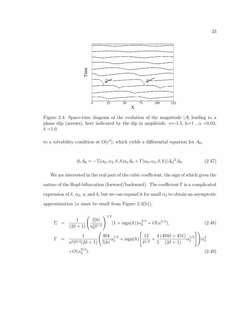
Figure 2.4: Space-time diagram of the evolution of the magnitude |A| leading to aphase slip (arrows), here indicated by the dip in amplitude. s=-1.5, h=1 , α =0.02,δ =1.0

to a solvability condition at O(ε3), which yields a differential equation for A0,

∂τA0 = −Σ(a0, α2, δ, h)a2A0 + Γ(a0, α2, δ, h)|A0|2A0. (2.47)

We are interested in the real part of the cubic coefficient, the sign of which gives the

nature of the Hopf-bifurcation (forward/backward). The coefficient Γ is a complicated

expression of δ, α2, a, and h, but we can expand it for small α2 to obtain an asymptotic

approximation (α must be small from Figure 2.3(b)),

Σ =1

(2δ + 1)

(

2|h|a3

0δ1/2

)1/2

(1 + isgn(h))α3/42 +O(α5/4), (2.48)

Γ =1

a2δ3/2(2δ + 1)

(

404

5|h|α1/22 + isgn(h)

[

12

δ1/2+

4

5

(494δ + 451)

(2δ + 1)α

1/22

])

α32

+O(α9/42 ). (2.49)

24

Thus in the limit α2 → 0, Re(Γ)> 0 for all values of the coefficients, and the phase

mode undergoes a backward Hopf-bifurcation. Solving the coefficient Γ numerically

over a wide range of parameter values always yielded a positive real part. This

analysis does not indicate whether or not the instability saturates at higher order or

if the phase becomes undefined, signaling a phase slip. To investigate the nonlinear

behavior of the phase, (2.7, 2.8) were integrated numerically using a linearized Crank-

Nicholson scheme. It was found for the parameter values tested, that the waves

outside the stability band underwent a phase slip when perturbed, relaxing to the

plane-wave- stable band as seen in Figure 2.4, which shows a space-time diagram of

the magnitude |A| of the waves.

2.4 Amplitude Instability: Modulated Waves

We now investigate the instability corresponding to the eigenvalue of the C-field pass-

ing through zero in (2.21), which occurs only for β > 0. Figure 2.5(a) indicates that

plane waves are stable at onset, becoming linearly unstable as the control parame-

ter is increased until , for large enough values of the control parameter, they once

again regain stability. In addition, the band of stable wavenumbers is bounded by

the Eckhaus curve outside the range of the amplitude instability. Thus for β > 0 two

distinct instabilities are possible, depending on the wavenumber of the waves and the

distance from threshold. Figure 2.5(b) shows the relevant eigenvalue as a function

of the modulation wavenumber for increasing values of the control parameter. The

wavenumber of the fastest growing mode increases continuously over the range of

values of the control parameter for which the waves are linearly unstable.

25

0 0.2 0.4 0.6Wavenumber q

0

0.2

0.4

0.6

a SW

SW

LW

LW

Plane Waves

PhaseInstability

Amplitude InstabilityModulated Waves

SW

Phase Slip

(a) 0 0.1 0.2Modulation Wavenumber p

-0.01

-0.005

0

0.005

0.01

σa = 0.025 a = 0.29

(b)

σfield

σfieldσ

phase

Figure 2.5: A linear stability diagram is given in (a) for h=1, s=1, α=0.02, δ=1.5. LWand SW denote longwave and shortwave instabilities respectively. In (b) the largestpositive eigenvalue of the system is plotted versus the modulation wavenumber atbandcenter. Shortwave instabilities occur as the control parameter a is increasedfrom the stable region near onset of the plane waves and as a is decreased from thestable region far beyond threshold.

At bandcenter, the system (2.9, 2.10, 2.11) decouples in the case of unperturbed

plane waves. Perturbing the plane-wave solution with the ansatz (2.12, 2.13, 2.14)

where q = 0, introduces a quadratic coupling of the phase to the real amplitude

through (∂xθ)2, which does not appear in the linearized system. Thus it is sufficient

to consider the following equations for the linear stability of the waves at bandcenter,

∂tR = ∂2xR +R[(a+ C) −R2], (2.50)

∂tC = δ∂2xC − αC + s∂xC + 2hR∂xR. (2.51)

Linearizing about the plane-wave solution in the above equations yields, for spa-

tially periodic modulations, a complex, quadratic polynomial in the growth rate σ.

As in section 3, setting σr = 0 gives a value for the Hopf-frequency,

26

ωHopf = p(2a(s+ h) + sp2)

((2a+ α) + (1 + δ)p2), (2.52)

and a polynomial in p, the roots of which give the values of the critical modulation

wavenumber,

−p2(2a(s+ h) + sp2)2 + sp2(2a(s+ h) + sp2)((2a+ α) + (1 + δ)p2)

+(p2 + 2a)(δp2 + α)((2a+ α) + (1 + δ)p2)2 = 0. (2.53)

For given values of the parameters, (2.53) must be solved for the critical modulation

wavenumber pcr implicitly. Requiring additionally that ∂σr

∂p= 0 allows us to determine

the value of the control parameter a for which the eigenvalue first passes through zero

as p is varied. We denote this value as ao.

If we are to solve (2.9),(2.10),(2.11) to higher order, we must consider the coupling

of the phase to the amplitude. We take an expansion of the form,

R

θ

C

=

√a0

0

0

+ ε

R0

θ0

C0

+ ε2

R1

θ1

C1

+ . . . (2.54)

Substituting this into (2.10) yields the following series of equations for the phase,

27

∂tθ0 = ∂2xθ0, (2.55)

∂tθk = ∂2xθk + ∂x

(

k−1∑

n=1

1

n!

∂n(R2)

∂εn(ε = 0)εn

)

∂xθj, (2.56)

where n + j = k and k > 0. Thus to leading order the phase satisfies the constant

coefficient diffusion equation. Higher orders include a forcing term proportional to

the gradient of all lower order terms, which must all decay to zero for long times due

to (2.55). We conclude that the long-term behavior of small-amplitude instabilities

at bandcenter will not be affected by the phase and consider (2.50, 2.51) the relevant

dynamics.

Weakly Nonlinear Analysis

In order to capture the dynamics of the instability near onset at both extremes of

the unstable band in the control parameter, we carry out a weakly nonlinear anal-

ysis. Since solving the polynomial (2.53) for the critical modulation wavenumber is

intractable we leave p as an implicit variable.

We again introduce a slow time scale τ = ε2t and define the distance from onset

ε =√

(a−a0)a2

. We consider a small-amplitude expansion,

R

C

=

√a0

0

+ ε

[

R0

C0

A0(τ)e

i(pcrx+ωcrt) + c.c+ h.o.t.

]

,

and systematically arrive at a solvability condition at order O(ε3) which yields a

28

0 0.1 0.2 0.3

Control Parameter a

0

0.2

0.4

0.6

0.8

1

|A|

(a) 0 50 100

X

-0.2

0

0.2

0.4

0.6

0.8

1|A|

max

|A|min

(b)

C

|A|

a = 0.15

1 1.2 1.4 1.6 1.8 2

δ

0.8

1

1.2

1.4

h

(A) (B) (C) (D)

backward

forward

(c) 0.02 0.022 0.024 0.026 0.028

Control Parameter a

0

0.2

0.4

0.6

0.8

1

|A| m

odul

ated

wav

e

(d)

(A) (B) (C) (D)

Figure 2.6: (a) Bifurcation diagram of modulated waves. Diamonds indicate minimaand maxima of a single-wavelength modulation, squares and circles two and threewavelengths respectively. Solid symbols indicate the point at which the correspond-ing mode linearly destabilizes the traveling wave (triangles indicate four-wavelengthinstability although solution branches are not shown). Parameter values are s=1,h=1, δ=1.5, α=0.02 with a system size L=125. (b) Solution with 2-wavelength mod-ulation. (c) Switch of the bifurcation from backward to forward according to (2.57).(d) Comparison of the results from the amplitude equation (solid lines) to numericalsimulations confirms this transition. Enough data points where taken for (A),(B) toindicate the presence of bistability and thus confirm the subcritical nature of the bi-furcations. s=1, h=1, α=0.02, and δ=1.1 (triangles),1.2 (diamonds),1.4 (circles),1.5(squares) with a system size L=62.5.

differential equation for A0,

∂τA0 = Λ(a0, α, δ, h, s; p(a0, ..))a2A0 + Π(a0, α, δ, h, s; p(a0, ..))|A0|2A0. (2.57)

29

0 50 100X

Tim

e

Figure 2.7: Space-time diagram of |A| showing the annihilation of one ’hump’ byanother leading to the formation of a single-wavelength modulated pattern from atwo-wavelength pattern. s=1, h=1, α=0.02, δ=1.5, a=0.04

The coefficients Λ and Π in (2.57) must be solved numerically by determining

the value of p from (2.53) for given values of the parameters. For the values of the

parameters tested, it was found that the secondary bifurcation encountered first as

the control parameter a is increased from 0 can be either forward or backward (cf.

stability island including a=0 in Fig. 2.5(a)). The bifurcation which occurs as a is

decreased from the region of stability of the plane waves was, in all cases, supercritical.

A bifurcation diagram for the modulated waves is given in Figure 2.6(a) for a system

size of L=125. The particular structure of the cascade of bifurcations is a consequence

of the finite system size, where each branch corresponds to a discrete number of

wavelengths of the modulation. The bifurcation to modulated waves near onset of

the traveling waves (for small a) is examined in detail in Figures 2.6(c),(d) where the

amplitude equation is compared to numerical simulation. As δ is decreased for fixed

values of the other parameters, the bifurcation switches from forward to backward.

30

-0.2 -0.1 0 0.1

Control Parameter a

0

0.5

1

1.5

2

|A|

(a) 100 150 200

X

0

1

2

3

4

(b)

|A|

C

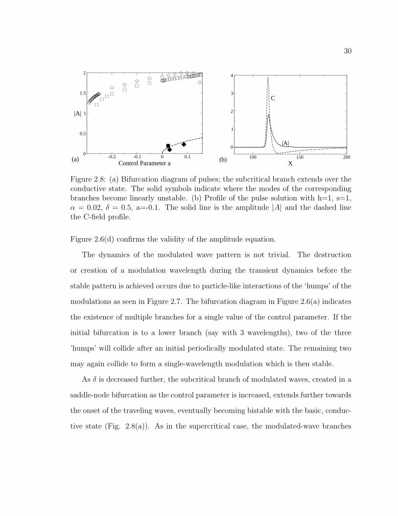
Figure 2.8: (a) Bifurcation diagram of pulses; the subcritical branch extends over theconductive state. The solid symbols indicate where the modes of the correspondingbranches become linearly unstable. (b) Profile of the pulse solution with h=1, s=1,α = 0.02, δ = 0.5, a=-0.1. The solid line is the amplitude |A| and the dashed linethe C-field profile.

Figure 2.6(d) confirms the validity of the amplitude equation.

The dynamics of the modulated wave pattern is not trivial. The destruction

or creation of a modulation wavelength during the transient dynamics before the

stable pattern is achieved occurs due to particle-like interactions of the ‘humps’ of the

modulations as seen in Figure 2.7. The bifurcation diagram in Figure 2.6(a) indicates

the existence of multiple branches for a single value of the control parameter. If the

initial bifurcation is to a lower branch (say with 3 wavelengths), two of the three

’humps’ will collide after an initial periodically modulated state. The remaining two

may again collide to form a single-wavelength modulation which is then stable.

As δ is decreased further, the subcritical branch of modulated waves, created in a

saddle-node bifurcation as the control parameter is increased, extends further towards

the onset of the traveling waves, eventually becoming bistable with the basic, conduc-

tive state (Fig. 2.8(a)). As in the supercritical case, the modulated-wave branches

31

arise from an instability of the plane-waves to finite wavenumber modulations. Modu-

lation wavenumbers p which lie in the interval pl < p < pu, where the bounds depend

on the value of the control parameter a, will linearly destabilize the plane-waves.

For a finite system of length L, there will exist modulated-wave branches for all n

such that p = 2nπL

lies in this interval. As n is decreased, the solutions increasingly

take on the characteristics of localized objects (Fig. 2.8(b)). In fact, the distance

between them can become arbitrarily large. Consequently, this distance can be much

larger than the maximal wavelength 2πpl

of modulations that linearly destabilize the

traveling waves in a given system. Thus, these solutions do not bifurcate directly

from the plane-wave branch but rather most likely arise in a tertiary bifurcation off a

modulated-wave solution. For example, Figure 2.9 shows a series of modulated-wave

branches for a system (L=250) where a single modulation (n = 1) does not linearly

destabilize the waves. Still, the single-pulse solution exists (dash-dot branch).

2.5 Conclusion

Systems similar to (2.7),(2.8) have been derived in various contexts, including a model

of traveling interfacial waves in two-layer Couette flow [8], where α = 0 due to conser-

vation of the additional zero-mode, given by the position of the interface. This system

was shown to exhibit a phase-instability leading to a phase-slip [7] in agreement with

experiment [1]. A small-amplitude model for traveling waves in thermal, binary-

mixture convection consists of complex Ginzburg-Landau equations for counterprop-

agating waves coupled to a slowly decaying mode representing large-scale variations

of the concentration field [4]. In this system, the traveling waves arise in a backward

32

-0.25 -0.2 -0.15 -0.1 -0.05 0

Control Parameter a

0

0.2

0.4

0.6

0.8

1

1.2

1.4

1.6

1.8

2

|A|

23 4

56 7 8 9 10 11 12

Single Pulse Branch

Figure 2.9: Bifurcation Diagram with h=1.0, s=1.0, α=0.02, δ=0.5, q=0 and L=250.Each branch represents a modulated-wave solution with the number of modulationsgiven. As this number n decreases, the modulated-waves become more like localizedtraveling pulses.

bifurcation. Localized pulse solutions arising from instabilities of this system were

identified and many of their properties characterized [17].

In this chapter we have shown that the advected mode can cause the phase-

instability to occur at finite wavelength and can introduce an additional amplitude-

instability. The latter is identified as the origin of pulse-solutions seen in earlier works.

They arise when the secondary bifurcation to modulated waves is sufficiently subcrit-

ical to lead to bistability between the modulated wave and the basic state. A similar

bifurcation may explain the appearance of localized “worms” in electroconvection in

nematic liquid crystals, seen again before the primary instability to supercritical trav-

eling waves. Indeed, a model of traveling waves coupled to a slowly decaying field has

been invoked to describe the worm dynamics, attaining qualitative agreement [14].

Finally, it would be worthwhile to consider the effect of dispersion in (2.7) on

the dynamics discussed in this chapter. In some cases dispersion has been shown

33

to have a significant effect on the linear-stability properties of waves coupled to a

additional mode. A model similar to (2.7, 2.8) used by Bartelet and Charru [1],

with α = 0 and added dispersion, seems to explain qualitatively the linear-stability

properties of waves observed in experiment. The inclusion of dispersion also allows for

a determination of the effect of the additional mode on the Benjamin-Feir instability.

In some cases this effect is important as, for example, in the 4-species Oregonator

model [5] of the BZ reaction where the Benjamin- Feir instability can be preceded by

a finite-wavenumber instability.

Chapter 3

Modulated Rotating Convection

3.1 Overview of Rotating Convection

Pattern formation in thermal convection of a rotating fluid layer has been the sub-

ject of much experimental and theoretical work in recent years. The effect of the

Coriolis force on the dynamics of thermal instabilities makes this system relevant for

both astrophysical and geophysical fluid dynamics, while the appearance of spatio-

temporally chaotic dynamics near onset make it an attractive candidate for detailed

analytical and numerical investigations of the origin and behavior of chaotic complex

patterns.

Kuppers and Lortz [19] determined that for rotation rates Ω greater than a critical

value Ωcr, steady convective roll patterns are unstable to another set of rolls oriented

at an angle β relative to the first. These results were confirmed and extended by

Clever and Busse [20], who also determined the dependence of Ωcr and β on the

Prandtl number of the fluid. In an infinite system, these dynamics are persistent

34

35

due to isotropy. Busse and Heikes [21] used this fact, and the closeness of β to π3,

to derive three coupled amplitude equations, in which rolls switch cyclicly as they

approach a heteroclinic orbit. In real systems, small amplitude noise perturbs this

orbit, leading to nearly periodic switching of rolls. In sufficiently large systems the

switching becomes incoherent in space and causes the development of patches of rolls

with different orientations. The ensuing dynamics are chaotic [22, 23].

In recent experiments on rotating convection [24], Thompson, Bajaj and Ahlers

investigated the effect of a temporal modulation of the rotation rate on the Kuppers-

Lortz (KL) state. They find that for sufficiently large modulation concentric roll

patterns (targets) as well as multi-armed spirals can be stabilized and replace the

chaotic KL state. Focusing on the target pattern, they find that the rolls in these

patterns drift radially inward and they measure the dependence of the drift velocity

on modulation amplitude and frequency, mean rotation rate, and heating. They

point out that the modulation sets up an oscillatory azimuthal mean flow, which

tends to align rolls along that direction. Since the alignment singles out a specific

orientation, it breaks the isotropy of the system. Motivated by these findings we

therefore investigate here the effect of anisotropy on roll patterns in systems exhibiting

KL chaos.

Within the framework of a suitably extended Swift-Hohenberg-model (SH) we

first study the stability of straight rolls in systems with broken chiral symmetry

(modeling the Coriolis force due to rotation) and with weak anisotropy. We then

use these analytical results to interpret simulation of this SH-model in a cylindrical

geometry in which we obtain target and spiral patterns as seen in experiment.

36

3.2 The stability of rolls with anisotropy

We study the effect of weak anisotropy on the Kuppers-Lortz state in the following

modified Swift-Hohenberg model,

∂tψ = µψ + α2(n · ∇)2ψ − (∇2 + 1)2ψ − ψ3 + γk · [∇× [(∇ψ)2∇ψ]], (3.1)

where n is a director indicating the preferred orientation, and α gives the strength

of this anisotropy. We retain the up-down (Boussinesq) symmetry (ψ → −ψ ) by

including only odd terms in ψ, and include a nonlinear gradient term that breaks

the chiral symmetry. The rotation rate is therefore measured by γ. Similar models

have been systematically derived from the fluid equations, with [25] and without

[26, 27] mean flow effects, and have enjoyed widespread use, e.g. [28, 29, 30, 31]. We

mean (3.1) to be a model equation and are concerned with the qualitative effect of

anisotropy on the Kuppers-Lortz instability.

Focusing on the weakly nonlinear regime and assuming the anisotropy to be weak,

we take µ = ε2µ2 and α = εα2 with ε 1. To leading order in ε the system is therefore

isotropic. To study the effect of the anisotropy on the KL-instability we consider the

weakly nonlinear competition of two sets of rolls with relative angle β with the ansatz,

ψ = ε(A(τ)ei(cos(θ)x+sin(θ)y) +B(τ)ei(cos(θ+β)x+sin(θ+β)y) + c.c.) + h.o.t. (3.2)

Thus here we do not analyze all side-band instabilities. To leading order the system

is isotropic and θ is a free parameter. The complex amplitudes A and B evolve on

the slow timescale τ = εt. For concreteness we take n = ey. At order ε3, a solvability

37

condition yields

∂τA = µ2A− α2 sin2(θ)A− 3|A|2A− (6 + 4γ sin β cos β)|B|2A, (3.3)

∂τB = µ2B − α2 sin2(θ + β)B − 3|B|2B − (6 − 4γ sin β cos β)|A|2B. (3.4)

We examine the stability of rolls of orientation θ with respect to a set of rolls

oriented β to the first set of rolls. With α = 0 (isotropic case), the absolute orienta-

tion of the rolls θ is irrelevant, and we find they become first unstable to rolls with

orientation

βKL = 45o (3.5)

for

γ ≥ γKL =3

2. (3.6)

Introducing α 6= 0 leads to a dependence of both βKL and γKL on the absolute

orientation of the rolls θ. The growth rates of the perturbations are given by

σA = −2(µ2 − α2 sin2 θ), (3.7)

σB = µ2(−1 +4

3γ sin β cos β) − α(sin2 θ + β + [

4

3γ sin β cos β − 2] sin2 θ).(3.8)

As can be seen from (3.7), the anisotropy has shifted the onset of rolls with

orientation θ to

µ2(θ) = α22 sin2 θ. (3.9)

Thus rolls with orientation θ exist for µ2 > µ2cr(θ). For fixed µ this implies a neutral

curve α(θ) as shown by the dashed line in Figure 3.1. Rolls of orientation θ first

38

Figure 3.1: Linear stability diagram of rolls with orientation θ in (3.3, 3.4) withrespect to rolls at a relative orientation of βKL. Here µ = 0.2. Numerical results aregiven by the solid symbols: triangles for γ = 3 and circles for γ = 2.

become unstable to rolls of different orientation at

σB =∂σB

∂β= 0. (3.10)

Equation (3.10) is solved here numerically for the linear stability limits although

it has been shown in [32] that the stability boundary can be found analytically.

Results are given in Figure 3.1 1 for various values of γ (solid lines). To test these

stability results we perform numerical simulations using a pseudospectral code with

periodic boundary conditions, employing an integrating factor Runge-Kutta time-

stepping method. We perturb straight rolls of orientation θ by small-amplitude rolls

of orientation θ + β, where β is chosen as the angle corresponding to the maximal

growth rate according to (3.10). To verify that no additional instabilities are present,

1The linear stability curve published in [33] is incorrect as pointed out by the authors in [32].The corrected stability curves are given in this figure.

39

Figure 3.2: Stabilization of rolls in the regime of domain chaos arising from theKuppers-Lortz instability. a) A typical patch-work pattern of domain chaos, wherethe angle between patches βKL = 45, and γ = 2.0, µ = 0.2, α = 0.0). b) For the samevalues of the parameters with α2 = 0.15, rolls are stabilized.

we also perturb the rolls with small-amplitude noise. As can be seen from the solid

symbols in Figure 3.1, numerical simulations agree well with the weakly nonlinear

analysis for rotation rates γ that are not too far above γKL(α) ∼ 1.5, for which

only weak anisotropy is needed for stability. For larger rotations rates γ, the weakly

nonlinear theory overestimates the amount of anisotropy α needed to stabilize rolls.

For α = O(1), the anisotropy affects the linear growth rate of rolls already in (3.1) and

will introduce a significant dependence of the critical wavenumber on the orientation

θ. Numerical results for larger α reveal that large amplitude rolls (with θ = 0) tend to

grow and invade regions of rolls of other orientations front-wise. In fact, for α → ∞

only rolls with θ = 0 exist.

Thus, weak anisotropy can stabilize periodic rolls arising in rotating convection

in the Kuppers-Lortz unstable regime. Specifically, there is a finite band of angles θ

with respect to the anisotropic director n such that rolls with this angle are stable to

homogeneous perturbations of all possible orientations.

40

3.3 Modulated rotating convection: spirals and tar-

gets

We now turn to the specific problem of rotating convection with periodically modu-

lated rotation. A thin layer of fluid of height d is heated from below and bounded

above and below by a rigid plate, which is rotated with an angular velocity Ω =

Ωo(1 + δ cosωt). For δ = 0 we recover the well-studied case of rotating convection

[19]-[25], [28, 29, 34]. For δ 1 but nonzero, a nontrivial base flow is induced by

the periodic motion of the rigid plates. This flow advects perturbations leading to

thermal instabilities in such a way as to affect their growth rate. Indeed, far from the

axis of rotation, the onset of the thermal instability is dependent on the orientation of

periodic-roll perturbations with respect to the base flow in a manner analogous to the

linear operator in (3.1) as discussed below, (cf. [35]). Closer to the axis of rotation,

the curvature of the base flow becomes significant and a straight-roll approximation

is not a good one.

The dynamics can be described by the Boussinesq fluid equations in a frame

rotating at the mean angular velocity Ω0 [19]-[23]. Due to the temporal modulation

of the angular velocity, the rigid boundary conditions at top and bottom imply that

the azimuthal velocity component oscillates in time with the plates,

uθ = <(δΩ0reiωt). (3.11)

This condition induces an azimuthal shear flow, the strength of which grows with

distance from the axis of rotation. If we assume the flow is restricted to a finite

41

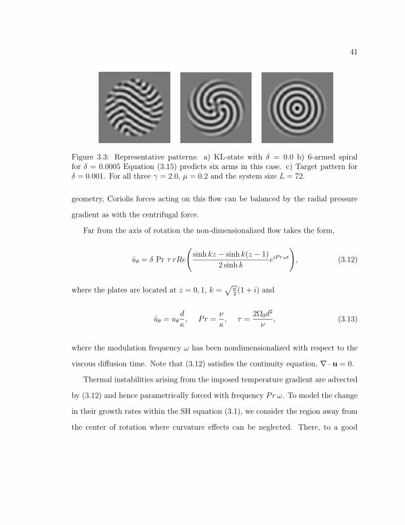
Figure 3.3: Representative patterns: a) KL-state with δ = 0.0 b) 6-armed spiralfor δ = 0.0005 Equation (3.15) predicts six arms in this case. c) Target pattern forδ = 0.001. For all three γ = 2.0, µ = 0.2 and the system size L = 72.

geometry, Coriolis forces acting on this flow can be balanced by the radial pressure

gradient as with the centrifugal force.

Far from the axis of rotation the non-dimensionalized flow takes the form,

uθ = δ Pr τ rRe

(

sinh kz − sinh k(z − 1)

2 sinh keiPr ωt

)

, (3.12)

where the plates are located at z = 0, 1, k =√

ω2(1 + i) and

uθ = uθd

κ, Pr =

ν

κ, τ =

2Ω0d2

ν, (3.13)

where the modulation frequency ω has been nondimensionalized with respect to the

viscous diffusion time. Note that (3.12) satisfies the continuity equation, ∇ · u = 0.

Thermal instabilities arising from the imposed temperature gradient are advected

by (3.12) and hence parametrically forced with frequency Pr ω. To model the change

in their growth rates within the SH equation (3.1), we consider the region away from

the center of rotation where curvature effects can be neglected. There, to a good

42

approximation, the analysis of section II should apply locally with the anisotropy

director n being given by the local orientation of the oscillating base flow, n = eθ.

This is based on the observation that near onset the dynamics of the instability is

slow compared with the period of the oscillating shear-flow for any finite rotation rate,

which allows an averaging over the oscillations. Since the forcing is invariant under

the transformation δ → −δ, t → t + πPr ω

, the base flow affects the growth-rate of

thermal instabilities through mean-squared contributions (proportional to δ2). Based

on (3.12) we therefore choose

α2 = δ2r2, n = eθ. (3.14)

We note that the scaling of the anisotropy (3.14) as linear in the distance from the axis

of rotation is only correct far from the axis itself. However, we retain this simplified

form and hope to extract qualitatively correct results. In fact, simulations with other

polynomial dependencies have revealed that only the monotonicity of the function is

important in determining qualitative features of the patterns.

To model the circular container of the experiments we use a circular ramp in

the control parameter µ, maintaining the region surrounding the circle at a sub-

critical value, thereby suppressing the convection amplitude. In full Navier-Stokes

simulations this procedure has been used successfully in comparison with experiment

(Pesch/Ahlers/Schatz). Simulations reveal a wide variety of spiral patterns as well

as targets. For small δ, where we expect the weakly-nonlinear theory for periodic

rolls to be valid sufficiently far from the core of the spiral, we are able to predict the

number of spiral-arms with reasonable accuracy. Such an analysis can be understood

43

from Figure 3.1. For a fixed ’rotation-rate’ γ, the strength of anisotropy α increases

with distance from the core of the spiral. There is thus a region in the vicinity of

the core where no rolls are stable, and rolls of a given orientation θ∗ are selected at a

distance r∗ as determined by condition (3.10). The projection of the local wavevector

of the spiral onto the perimeter of the critical circle with radius r∗ is given by q sin θ∗.

The number of arms of the spiral is then given by the circumference (2πr∗) divided

by the wavelength associated with the projected wavevector,

N = r∗q sin θ∗. (3.15)

Spirals or targets can be generated for the same parameter values given different

initial conditions. In general, an initial straight roll pattern will result in a target

for sufficiently large δ, whereas disordered initial conditions generically yield spirals,

even for strong anisotropy.

Interestingly, the orientation-selection mechanism given by (3.15) predicts the

possibility of a large region surrounding the core, within which no rolls are stable in

the context of the weakly nonlinear theory. If the anisotropy is sufficiently weak, one

should see a disordered region of domain chaos, bounded by a stable spiral, given a

large enough system. Such a pattern is shown in Figure 3.4.

3.4 Conclusion

Spirals and targets arising in Rayleigh-Benard convection have been the subject of

much theory and experimental work, [25, 22, 29, 36, 37, 38]. Target patterns in low-

44

Prandtl number convection are a consequence of horizontal, thermal gradients at the

sidewalls of a cylindrical container, which tend to align rolls parallel to the walls [38].

Even with sidewall forcing, the targets become unstable to straight rolls relatively

close to threshold. In rotating convection, the target patterns arising from such

sidewall forcing undergo a mean drift [29] due to the breaking of reflection symmetry

by the applied rotation. However, in the case of rotating convection with a modulated

rotation rate, the chiral patterns are not a consequence of the system geometry, but

rather are induced by an isotropy-breaking shear flow, which acts azimuthally. We

have shown that these patterns are stable in regimes where one would see spatio-

temporal chaos in the absence of modulation. Our analysis indicates that the shear

flow acts to stabilize rolls within a band of stable orientations w.r.t. the azimuthal

flow itself. This leads naturally to a chiral pattern.

The qualitative agreement between the types of patterns observed in experiment

[24] and those studied here make the selection mechanism described in section III

plausible. Spirals and targets arise through the interaction of the destabilizing pro-

cess responsible for the KL instability and the stabilizing effect of the azimuthal

mean flow (MF). Quantitative comparison of the dependence of the pattern behavior

on the reduced Rayleigh number, rotation rate, and amplitude and frequency of the

modulation with experiment is, however, not possible within the framework of (3.1).

However, the qualitative genericity of the appearance of spirals patterns under modu-

lated rotation with disordered initial conditions (KL state) seems to hold both under

experimental conditions and here. Targets, on the other hand, must be generated

with care but then persist as stable patterns over a wide range of parameter values.

The target patterns observed in [24] travel inwards radially, collapsing periodically

45

Figure 3.4: A stable spiral with a chaotic core. The system size is L = 144 withγ = 2.0, µ = 0.2 and δ2 = 0.0001. Note that equation (3.15) predicts 14 arms. Thecore dynamics occur on a fast timescale w.r.t. the slow, solid-body rotation of theouter spiral.

at the center. The origin of this drift has not been identified yet. One possibility

is that the time-periodic component of the Coriolis force acting on the time-periodic

azimuthal flow generates a radial flow with a steady component, which would advect

the axisymmetric roll pattern [39, 40]. Another possibility is that the drift is due to

a mismatch between the wavenumber selected by the umbilicus [41] and that selected

by the container side-wall [42, 43]. The competing selected wavenumbers set up a

wavenumber gradient that induces a drift of the pattern [44, 45]. It should be possible

to distinguish between these two mechanisms by comparing the dynamics in systems

of different aspect ratio. For larger systems, the wavenumber gradient induced by the

incompatibility of the selected wavenumbers would be weakened, while the effective

strength of the radial flow would naturally be stronger due to the greater Coriolis

force at larger radii. Experiments in such larger systems would also be of interest

in view of the prediction that in such systems the core of the spirals would exhibit

chaotic dynamics of the Kuppers-Lortz type.

In our simulations of (3.1) no radial drift of the concentric rolls was found. This

46

is not unexpected, since in the absence of the chiral-symmetry breaking term propor-

tional to γ eq.(3.1) is variational and persistent dynamics are ruled out. To obtain

drift the variational character of the system has to be broken to a sufficient degree.

This may require much larger rotation rates γ or the introduction of additional non-

variational terms. We have not pursued this further since simulations of extensions of

(3.1) with possibly also modified boundary conditions would not allow any quantita-

tive comparison with experiments and would therefore be of limited use in identifying

the dominant mechanism responsible for the drift.

Chapter 4

Slip at a Liquid-Solid Interface

4.1 Evidence of slip

In the modeling of the flow of fluids past a solid interface one assumes that, at the

interface, the component of the fluid velocity tangential to the solid matches the

velocity of the solid itself. This is the no slip condition, and it successfully describes

the behavior of simple fluids at the macroscopic scale.

Increasingly, however, both experiments [46, 47, 48, 49, 50] and molecular dynam-

ics (MD) simulations [51, 52, 53, 54] indicate that slip does occur at the microscopic

scale. Pit, Hervet and Leger [46] measured the slip of hexadecane over sapphire and

concluded that molecular-scale roughness of the solid surface inhibited slip although

slip lengths up to 400nm were found. Zhu and Granick [47] investigated the flow of

Newtonian fluids over molecularly smooth surfaces and found that there is a critical

flow rate above which slip occurred. The degree of slip was furthermore correlated

with the wettability of the interface. Craig, Neto and Williams [48] found that the

47

48

slip of aqueous solutions of sucrose on mica depended both on the viscosity of the

fluid and the shear rate at the interface. Bonnacurso, Kappl and Butt [49] found slip

for water on hydrophilic surfaces with a slip length of 8-9nm, while Bonaccurso, Butt

and Craig [50] found that large-scale roughness of a completely wetting surface can

actually increase slip.

Thomson and Robbins [51] showed in MD simluations that the amount of slip was

correlated with the degree of ordering of the fluid particles at the solid interface. The

investigation of the effect of various densities and interfacial energies in simulations

by Thompson and Troian [52] revealed a universal relationship between the shear rate

at the interface and the slip length. Cieplak, Koplik and Banavar [54] concluded that

the ordering of the fluid near the interface was the determining factor in predicting

slip.

Most of the available data support the notion that slip will be understood only by

considering the molecular interaction between the fluid and the solid at the interface.

The organization of the initial fluid layer seems crucial to the question of slip and it

has been hypothesized that the mechanical properties of this layer are truly different

from the bulk properties of the fluid [49], i.e. a new phase.

The present study approaches the question of slip at a fluid-solid interface from a

dynamical-systems’ perspective. We propose the use of a well-known equation from

solid-state physics, the Frenkel-Kontorova (FK) equation, as a model of coherent

motion in the initial fluid layer at the interface. Parameters in the FK equation

can be meaningfully related to properties of the fluid and solid. A close look at slip

dynamics in MD simulations will then motivate some modification of the FK model,

the dynamics of which agrees remarkably well with the MD. The modified FK model

49

indeed describes the dynamics of a phase which is solid-like on short time scales, but

diffusive (fluid-like) on longer time scales.

4.2 The Frenkel-Kontorova Equation

We consider a chain of coupled molecules with an equilibrium interparticle spacing

of a. The chain sits a fixed distance d from the solid and is subject to a periodic

potential with spatial period λ. Particle i has an energy given by the Hamiltonian

H =∑

i

m

2

(

dxi

dt

)2

+ h[

1 − cos(2πxi

λ

)]

+k

2(xi+1 − xi − a)2

. (4.1)

From the Hamiltonian follows the equation of motion for the ith particle

mxi = −2πh

λsin(2πxi

λ

)

+ k(xi+1 − 2xi + xi−1) + ηff (V − xi) − ηfsxi (4.2)

where local dissipation of energy is modeled heuristically via a momentum transfer

between liquid particles, proportional to the horizontal component of the velocity

difference V − xi and a liquid to solid energy loss, here taken to be proportional to

the liquid particle velocity. The quantity V is thus taken to be a measure of the mean

velocity of the liquid particles just above the initial layer near the interface.

It is instructive to consider the limit of large shear rate for which the last two

terms in 4.2 will balance, yielding

xi =ηffV

ηff + ηfs

. (4.3)

50

Equation 4.3 is valid for all i, indicating that the slip velocity of the liquid particles

adjacent to the substrate is simply proportional to the mean horizontal component of

the velocity of those liquid particles near the wall in the bulk. The slip length, which

is defined as the fictional distance below the interface at which the liquid velocity

would equal zero if extrapolated linearly, is defined as the the slip velocity divided by

the shear rate Ls =vslip

V −vslipd. For large shear rates in 4.2 this is just

Ls =ηff

ηfs

d. (4.4)

In general, the shear stress at the interface can be written σfs = feffvslip where feff

is the effective friction between the liquid and solid [46]. The slip length Ls =vslip

γ

where γ is the shear rate, which itself can be written γ =σfs

ηbulk, where ηbulk is the bulk

viscosity of the liquid. Finally this yields

Ls =ηbulk

feff

(4.5)

Thus, comparison of 4.4 and 4.5 reveals that at least for large shear rates the

modified FK model yields a consistent and accurate estimate of the slip length. Fur-

thermore the parameters ηff andηfs

dcan be considered the bulk visocity of the liquid

and the effective liquid-solid friction respectively. Note, as mentioned earlier, that slip

increases with increasing liquid viscosity and shear-rate at the interface in experiment,

effects which are trivially captured in 4.2 as the forcing is just ηff (V − xi).

We consider two possible non-dimensionalizations of 4.2, which differ in the defini-

tion of the relevant time scale. In the first case we normalize time by the frequency of

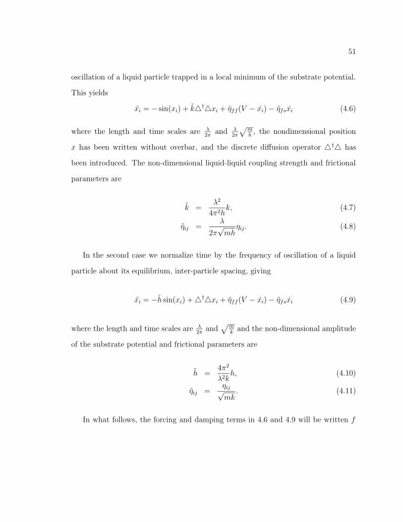
51

oscillation of a liquid particle trapped in a local minimum of the substrate potential.

This yields

xi = − sin(xi) + k4†4xi + ηff (V − xi) − ηfsxi (4.6)

where the length and time scales are λ2π

and λ2π

√

mh, the nondimensional position

x has been written without overbar, and the discrete diffusion operator 4†4 has

been introduced. The non-dimensional liquid-liquid coupling strength and frictional

parameters are

k =λ2

4π2hk, (4.7)

ηij =λ

2π√mh

ηij. (4.8)

In the second case we normalize time by the frequency of oscillation of a liquid

particle about its equilibrium, inter-particle spacing, giving

xi = −h sin(xi) + 4†4xi + ηff (V − xi) − ηfsxi (4.9)

where the length and time scales are λ2π

and√

mk

and the non-dimensional amplitude

of the substrate potential and frictional parameters are

h =4π2

λ2kh, (4.10)

ηij =ηij√mk

. (4.11)

In what follows, the forcing and damping terms in 4.6 and 4.9 will be written f

52

and ηxi where

f = ηffV, (4.12)

η = ηff + ηfs. (4.13)

Other non-dimensionalizations are possible, including scaling by a viscous diffusion

time , but we will restrict our analysis to 4.6 and 4.9, thereby retaining the damping

coefficients explicitly. Worthy of note is the conspicuous absence of the inter-particle

spacing a from 4.1. In fact, the value of the non-dimensional parameter ξ = aλ

plays

a crucial role in determining the dynamical state of the system defined by 4.2. The

commensurability parameter ξ measures the relative liquid-liquid to solid-solid inter-

particle spacings and strongly influences the degree of slip in the chain, as we shall

see.

Equation 4.2 is the forced, damped Frenkel-Kontorova (FK) equation. The FK

equation itself, which is obtained by setting ηff and ηfs to zero in 4.2, was first

introduced in the theory of dislocations in metals [55]. It has been evoked to describe

the motion of dislocations in crystals, the propagation of charge-density waves, the

theory of Josephson junctions and the molecular basis for solid friction as well as

many other important applications in solid-state physics [55, 56]. The universality of

the FK model resides in the fact that it is the simplest possible model of a chain of

coupled particles subject to a periodic potential.

In the limit that the inter-particle spacing goes to zero in the FK model, the

discrete operator can be expanded in the small parameter a. Retaining only the

53

leading order term yields the sine-Gordon (sG) equation

mu = −2πh

λsin(2πu

λ

)

+ c2u′′

(4.14)

where c2 = ka2

2and thus the equation is valid only for k → ∞. The variable u(x)

represents a displacement, which depends now continuously on the spatial variable

x. The equation 4.14 can be non-dimensionalized with U = 2πλu, X = 2π

λ

√

hc2x and

T = 2πλ

√

hmt, to yield

U − U′′

+ sinU = 0 (4.15)

The sG equation, together with other nonlinear equations such as the Korteweg

de-Vries (KdV) and nonlinear Schrodinger (NLS) equations is exactly integrable and

thus solvable by the inverse scattering method [57, 58]. Solutions of 4.14 include

small-amplitude phonon modes (radiation) as well as localized kinks and antikinks in

which the phase winds ±2π respectively. Time-varying kinks called ‘breathers’ are

also solutions of 4.14. The connection between kinks in the integrable sG limit and

dislocations or defects in the FK model is well-established [55] although key differences

make the two qualitatively distinct. In particular, kink solutions of 4.14 represent

Goldstone modes due to the translational invariance of the sG equation. As such no

energy is required to drive defects in the continuum approximation. In contrast, the

FK equation is invariant only under discrete translations, the physical consequence of

which is a pinning force that must be overcome to drive defect motion. Nonetheless,

perturbations of the continuum description can prove fruitful in elucidating properties

of kinks in discrete lattices.

54

4.3 Slip dynamics in the FK model

Analysis of the equilibrium states of 4.2 already provides a major theoretical challenge,

which has been taken up by many researchers (see [56] for a review). Using the non-

dimensional equation 4.6, determination of the equilibrium configuration of particles

is equivalent to solving

sin xi = k(xi+1 − 2xi + xi−1) + f (4.16)

where all overbars have been dropped. It should be noted in light of the motivation

for this work, that the equilibrium arrangement of liquid molecules at a solid interface

is not well understood even for water on a metal surface (e.g. [59]). A quantitative

description of these states requires a detailed understanding of the relevant forces,

which may well differ considerably depending on the solid and liquid properties. Given

these forces, the equilibrium configuration is just the minimal energy state, whose

determination in the FK model is equivalent to solving 4.16 1.

The liquid-liquid equilibrium interparticle spacing a is once again absent in 4.16.

It plays an indirect role in defining the average density of particles, e.g. if the system

length consists of 100 periods of the underlying substrate then the solution of 4.16

will clearly be different for 100 or 157 particles and is thus depedent on a in this way.

Let us first consider solutions of 4.16 with f = 0, which we will refer to as unforced

ground states. The nature of the ground states depends crucially on the commensu-

rability ξ, also referred to as the average spacing or winding number [56]. Ground

states are called commensurate for rational values of ξ and are otherwise called in-

1Solutions to the equation 4.16 will, of course, give saddle-point energy states as well.

55

Figure 4.1: Ground state of chain for which ξ = 23. The chain is invariant under the

discrete translation of one period of the underlying substrate. Taken from [56].

commensurate. All commensurate ground states are periodic with period Λ such that

Λ is the smallest integer for which Λξ

is also an integer. Figure 4.1 shows a ξ = 23

ground state for which Λ = 2 (Λξ

= 3). It is worth noting that 1ξ

= λa

= pq

where p is

the average number of particles over q periods of the substrate. In a one-dimensional

system this is proportional to the density of particles. For a fixed system size L with

q periods of the substrate of wavelength λ and p particles, the commensurability can

be rewritten

ξ =1

1 + (p−q)λL

(4.17)

where the quantity δ = (p−q)q

is known as the mismatch. The quantity | δλL| is the

density of defects.

The ground state shown in Figure 4.1 is clearly invariant under discrete trans-

lations of one period of the periodic potential. The consequence of this discrete

symmetry is the existence of a pinning potential which must be overcome to shift

the chain one unit. The pinning potential is related to the adiabatic trajectory con-

necting the two minima in the energy landscape given by the second two terms of

the Hamiltonian 4.1. The adiabatic trajectory refers to the trajectory along which

the system relaxes to its new energy state at each point, i.e. momentum may be

56

neglected. If the trajectory passes through a less energetically preferred state, then

some work must be done to shift the chain. Commensurate chains always exhibit

such a pinning potential known as the Peierls-Nabarro potential EPN . We then see

that given a nonzero f , there may or may not exist a solution to 4.16. Namely, for

f > EPN

λthe chain is unpinned and no static solutions exist.

In contrast to commensurate chains, ground states of incommensurate chains may

or may not be pinned. For k = 0 all the particles fall into the wells of the periodic

substrate regardless of the value of ξ. As the coupling strength increases, Aubry has

proven [60] that there is a transition at a critical value kcr(ξ) for which the pinning

potential goes to zero. Furthermore he proved that this occurs first for the value of

ξ that is “most irrational”:√

5+12

, the golden mean. The transition to the de-pinned

state is related to the emergence of a zero-mode of the linearized operator in 4.16

about the ground state [61], effectively making the system translationally invariant.

Thus for some incommensurate systems EPN must still be overcome to unpin the

chain, while for others the particles will move freely even for an infinitesimal value

of the forcing f . It should be noted that we consider a periodic system in which the

most incommensurate chain will still be periodic with period equal to the system size

itself.

Once the particles have begun to move along the substrate under the force f we

will find it useful to define the slip velocity

vslip = limT→∞

1

T

∫ T

0

dt1

N

N∑

i=1

xi, (4.18)

which is merely the long-time average of the ensemble average of particle velocities.

57

In practice 4.18 is calculated numerically with a finite T taken sufficiently large for

convergence.

Technically, characterizing the slip of the liquid particles in the context of 4.2

reduces to the following two problems:

1. Determine the critical value of the forcing fcr(ξ, k, η) at which slip first occurs.

2. For f > fcr, determine the slip velocity vslip(ξ, k, η, f − fcr).

We will look in depth at points 1 and 2 for the strongly damped (order 1, not

overdamped), driven FK model. This is particularly important since recent studies

have revealed quite complex dynamics in the weakly damped, driven FK model (η

small) [62, 63, 64, 65]. Strunz and Elmer [62] show that there is a parametric resonance

instability of the uniformly sliding chain if the damping is weaker than the amplitude

of the substrate potential. In addition, the weak damping leads to bistability between

flowing and static states. For weak enough damping, inertia is sufficient to maintain

the motion of the chain despite the existence of a stable ground state. This bistability

leads naturally to domains and fronts. For very weak damping (η 1) [63] the

dynamics is chaotic. It may be that weakly-damped dynamics is relevant for the

motion of liquid particle near a solid interface. One can make an argument for at

least order one damping given the relatively high temperature of a liquid. For the

sake of simplicity, we will not analyze the weakly damped dynamics in the present

study.

The connection between 4.2 and slip at a liquid-solid interface has been motivated

heuristically, but results from the FK model should be carefully scrutinized before

conclusions about real liquids are drawn. The FK equation is used here as a dy-

58

namical description of the tangential projection of liquid motion at a solid boundary.

Important omissions from a theory based solely on the FK equation include:

1. The second degree of freedom tangential to the interface (surfaces are 2-D).

2. The explicit dependence on the degree of freedom perpendicular to the interface.

With regards to 1, Braun and Kivshar [66] have addressed quasi-two-dimensional

motion in a model of transversely coupled FK chains in the continuum limit (k →

∞) and derive an effective Hamiltonian governing the transverse dynamics of kinks

(defects). This type of coupling may introduce some new dynamical effects. However,

in the context of slip, we expect that the relevant dynamics will be aligned with

the direction of forcing and that a 1-D approximation to the anisotropic system is

acceptable. Transverse particle diffusion should not qualitatively affect the results

presented here.

With regards to 2, the momentum transfer term in 4.2, ηff (V − xi), is a dis-

cretized shear rate at the interface and as such attempts to capture the velocity

gradient perpendicular to the interface. Nonetheless, particle motion perpendicular

to the interface may change the slip behavior qualitatively and cannot be explicitly

captured in 4.2. Only comparison with MD simulations can reveal to what extent the

perpendicular motion of the liquid particles is important. In fact, we shall see that

careful observation of the vertical flux in MD simulations will allow us to modify the

FK model to precisely address this second point.

The most interesting, and luckily most robust, prediction of this work is the

existence of two slip regimes: one defect-driven and the other, a bulk-slip regime.

The bottom line of all the results to follow is that as the forcing of the liquid particles

59

at the interface (e.g. shear rate) increases from zero, slip will generically occur first

due to localized dislocations, followed by a second transition to bulk slip. 2

In the following sections we will present an overview of the determination of

fcr(ξ, k, η) and vslip(ξ, k, η, f − fcr) in the damped, driven FK model, filling in blanks

where results have not been presented in the literature. We will then discuss the

results of MD simulations and compare them to those of a newly proposed, modified

FK model.

4.4 Commensurate chains with integer values of ξ

The dynamics of those chains for which ξ is an integer is equivalent to that of a single

particle. In this case the coupling term, in the absence of noise, is identically equal

to zero

xi = − sin xi + f − ηxi. (4.19)

It should be noted that if the particles are inhomogeneously spaced initially, then

the dynamics will exhibit a coupling-dependent transient. However, for sufficiently

long times, 4.19 will be an asymptotically correct description of the particle motion.

The dynamics of 4.19 are very simple. For f < 1 there are two equilibria given

by xeq = sin−1 f ; if xs and xu denote the stable and unstable equilibria respectively,

then xu = π − xs for 0 ≤ xs ≤ π/2. Note that 4.19 is also the equation of motion

for a forced pendulum, in which case xs is the pendulum hanging down and xu is the

position at which the pendulum can be balanced on end. As f approaches 1, the two

2As a note, the large degree of shear needed to reach the bifurcation to bulk slip may be physicallyunrealizable. We thus expect the defect-driven regime to be the dominant paradigm of liquid slip inthe regime where the present study is valid.

60

equilibria coalesce in a saddle-node bifurcation (SN) at xs = xu = π2, at which point

the energy barrier to particle motion vanishes. An equation of motion for the particle

near the SN (|f − 1| 1) is easily derived, yielding

x =f − 1

η+

1

2ηx2. (4.20)

Equation 4.20 is simply the normal form equation for a SN and clearly shows

the existence of two equilibria for f − 1 < 0. We can make use of the fact that the

motion is periodic (SN on a circle) by transforming the position x into a phase with

x(t) = tan(

θ(t)2

)

3. Plugging this into 4.20 gives

θ = ω + b cos θ (4.21)

with ω = 2f−1η

, b = 2f−3η

and −π < θ < π. This formulation takes advantage of the

fact that for f − 1 1 the particle spends most of its time near the SN point. Once

it escapes (x → ∞ as θ → π), it travels to the next ‘hill’ where it once again hangs

around the SN point and so on. Thus the time it takes for the particle to traverse

one period of the substrate can be approximated as

TSN =

∫ π

−π

dθ

ω + b cos θ, (4.22)

and the non-dimensional slip velocity is given by vslip = 2πTSN

. The solution of 4.22 is

3Interestingly, this bifurcation (SN on a circle) is also ubiquitous in single-neuron dynamics wherethe excursion to infinity is interpreted as an action potential. The resulting phase equation 4.21 isknown as the θ-equation for ‘class 1’ excitable neurons [67].

61

0 1 2 3 4f

0

0.5

1

1.5

2

v slip

numericalSNhigh shear

Figure 4.2: Chains for which ξ is an integer (here 20) exhibit a SN bifurcation at acritical shear rate. Here ηff = ηfs = 1, h = 1, λ = 2π and k = 1. Equation 4.2 wassolved with a 4th-order Runge-Kutta scheme and long-time averages were taken.

2π√ω2−b2

, which gives

vslip =

√2

η

√

f − 1. (4.23)

Finally, in dimensional variables

vslip =2π

λ

√

2

h

√

ληff V

2πh− 1

(ηff + ηfs). (4.24)

Thus, for integer values of ξ, the particles are trapped below a critical value of

the forcing (shear rate) beyond which the slip velocity increases like the forcing to

the 1/2 power. For large shear rates, 4.3 once again applies; see figure 4.2.

62

4.5 Commensurate chains with ξ near an integer

value

If we consider a chain with a value of ξ very close to an integer value (e.g. 100101

) we

see that the ground state of the system corresponds almost everywhere to that of

the respective chain with exactly the integer value. Only at a few points will the

addition (absence) of particles cause a contraction (expansion) of the chain. In the

case ξ = 100101

, there is one extra particle per one hundred periods of the potential,

referred to as a dislocation or defect.

In fact, we will see that a single defect in the undamped, unforced FK model cor-

responds to a kink (soliton) in the integrable limit (sG), and that the correspondence

is exact for k → ∞. Kink solutions [58] to 4.15 have the form

Uk(X,T ) = 4 tan−1

e−σ

(X−V T )√1−V 2

(4.25)

which in dimensional form (from 4.14) is

uk(x, t) =2λ

πtan−1

e− 2πσ

√h

cλ

(x−vt)√

1−mv2

c2

. (4.26)

The velocity of the kink V should not be confused with the velocity in 4.2 and is

distinguished here by the overbar.

Depending on the sign of σ = ±1, the kink 4.25 is a front solution twisting through

±2π. The velocity v is a free parameter indicating that there is no selected velocity.

63

In the case of the weakly forced, weakly damped sG equation

U − U′′

+ sinU = f − ηU (4.27)

where for f, η 1, a perturbation analysis yields a soliton solution which to leading

order is equal to the unperturbed soliton 4.26. At next order the velocity is uniquely

determined [57]. The steady-state value is

V =1

√

1 +(

4ηπf

)2, (4.28)

which in dimensional form is

v =a√

k2m

√

1 +(

4(ηff+ηfs)

πηff V

)2hm

. (4.29)

Let us now turn our attention once again to the FK model and consider the

quantity vslip defined by 4.18 as a function of the parameter ξ. As we see in figure

4.3, the slip is identically zero for the cases where ξ is an integer (we are just at the

SN bifurcation in a system of 100 periods of the underlying potential, i.e. ξ = 100/p

where p is the number of particles). The slip increases monotonically as ξ deviates

from integer values. Specifically, for a fixed value of k, the slip velocity increases

initially linearly as a function of 1/ξ. In this regime, the density of defects is low

(see 4.17) and the slip velocity is therefore simply proportional to this density. As

the density of defects increases, they begin to interact with one another and the slip

64

0.1 11/ξ

0

0.1

0.2

0.3

0.4

0.5

Vsl

ip

k=0.1k=0.5k=1.0k=2.0

Figure 4.3: Slip velocity vs. 1ξ. The number of periods of the substrate is 100 and

the number of particles in the chain increases from left to right. Parameter valuesare as in figure 4.20 except for the forcing V which is fixed at 1. All curves go to zeromonotonically as ξ → 0. Lines are meant as guides to the eye only.

velocity deviates from a linear dependence. Finally, for ξ sufficiently far from an

integer value, individual defects are not discernible and the dynamics is described by

a dynamic hull-function, discussed below. Also, for a fixed value of ξ, the slip velocity

increases as the coupling k increases.

Note that here, given ηff = ηfs = V = 1, the maximum possible slip velocity

is 12. For larger values of 1/ξ (ξ → 0) all curves approach zero monotonically. In

fact, as ξ decreases for a fixed system size, the number of particles increases. The

case ξ → 0 is then the limit in which the interparticle spacing goes to zero, i.e. the

continuum limit. A simple bifurcation anaylsis of the forced, damped sine-Gordon

equation shows that the SN bifurcation at f = 1 is once again recovered, i.e. the slip

goes to zero for f ≤ 1.

65

0 0.2 0.4 0.6 0.8 1f

0

0.005

0.01

0.015

0.02

0.025

0.03

v slip

0 0.2 0.4 0.6 0.8 1k

0

0.2

0.4

0.6

0.8

1

f cr

Eqn (3.33)Eqn (3.37)Eqn (3.39)

Figure 4.4: Inset: Slip velocity vs. force for a single defect for various values of the cou-pling k = 0.01 − 0.1 in increments of 0.01 then k = 0.15, 0.2, 0.3, 0.4, 0.5, 0.6, 0.7, 0.8.Slip increases for increasing k. Main: Depinning force vs. coupling k for a singledefect.

The inset of 4.5 shows the region near an integer value of ξ. Equation 4.29 predicts

the velocity of a kink should increase as k12 . If we normalize curves for different k’s

by this factor there is good collapse, as seen in the main panel of figure 4.5. Note

that 4.29 is for weakly driven, weakly damped kinks in the continuum limit. Despite

this, it captures the correct scaling for coupling strength even for strongly driven,

strongly damped kinks in the discrete system. For values of ξ not too far from one

we expect the defects to be far apart from one another (dilute limit) and thus not

interact strongly. Then the average slip should be approximately proportional to the

number of defects. The curves in figure 4.5 are linear near ξ = 1, in agreement with

the notion that the defects interact weakly.

Figure 4.3 shows the average velocity of the chain for a fixed value of the forcing.

66

0.9 0.95 1 1.05 1.10

0.1

0.2

0.3

0.4

0.5

Vsl

ip

k=0.1k=0.5k=1.0k=2.0k=3.0

0.9 0.95 1 1.05 1.11/ξ

0

0.2

0.4

0.6

0.8

Vsl

ip/s

qrt(

k)

λ/a

Figure 4.5: Inset: ξ near 1 from figure 4.3. Main: Curves rescaled by the predictedsoliton dependence on coupling given by 4.26.

We have seen that for integer values of ξ there is a SN bifurcation to slip at a crit-

ical value of the forcing, below which there is no motion. We may ask, given that

noninteger values of ξ lead to slip already below this SN bifurcation, whether chains

with defects also exhibit a bifurcation to motion, or if any force is sufficient to move

the defect. The answer is already given by the discrete translational symmetry of the

defect. It is invariant under translations of one period and therefore feels a pinning

force. We can determine this pinning force explicitly in the limits of weak and strong

coupling (c.f. figure 4.4).

For k 1 we solve for the stable and unstable configurations of the ground-state

of a single, forced kink evolving according to 4.2, by assuming that deformations of the

chain are localized near the kink position. Once we have solved for the ground state

(xi’s) we can determine the energy of the kink from the Hamiltonian 4.1. Schematic

67

S

U

S

U

f

Figure 4.6: Schematic stable and unstable configurations for weakly-coupled kinks.Left: Unforced. Right: forced.

ground states are shown in figure 4.6. For f sufficiently far from 1 (f must be at least

order k from the SN bifurcation to bulk slip) this yields

Es = N(1 −√

1 − f 2) + 2kπ2 + O(k2) (4.30)

Eu = N(1 −√

1 − f 2) + 2√

1 − f 2 + kπ2 + 4kψ(

ψ − 2f√

1 − f 2

)

+O(k2) (4.31)

where N is the number of particles in the chain and ψ = sin−1 f . Taking the difference

between these two energies gives the Peierls-Nabarro potential

EPN(f) = 2√

1 − f 2 − kπ2 + 4kψ(

ψ − 2f√

1 − f 2

)

+ O(k2). (4.32)

In the limit f → 0 one recovers the classical result [55]

EPN(0) = 2 − kπ2 + O(k2) (4.33)

68

From the energy 4.32 we can calculate the critical forcing at which the defect will

first move

fcr =EPN(fcr)

λ. (4.34)

Unfortunately, while 4.32 gives the asymptotically correct energy for small k, it breaks

down near f = 1. Figure 4.4 shows the predicted fcr using 4.32.

We can alleviate this problem by considering next-order corrections to the ground-

state positions of the particles. In this case we expand f near 1 (f = 1 − εf), which

leads to different zeroth order terms. This gives

Es = N(1 −√

1 − f 2) + 2π2k + 2√

2(1 − f)

−√

2(1 − f)

(√

1 +2πkf

1 − f+

√

1 − 2πkf

1 − f

)

+ O(k3/2) (4.35)

Eu = N(1 −√

1 − f 2) + k(π2 + 4ψ2) + 2√

1 − f 2

+√

2(1 − f)

(

1 +

√

1 − 4kfψ

1 − f−√

1 +kf(π + 2ψ)

1 − f

−√

1 − kf(π − 2ψ)

1 − f

)

+ O(k3/2). (4.36)

The Peierls-Nabarro potential is then

EPN = 2√

1 − f 2 − k(π2 − 4ψ2) −√

2(1 − f) +√

2(1 − f)

(√

1 − 4kfψ

1 − f

−√

1 +kf(π + 2ψ)

1 − f−√

1 − kf(π − 2ψ)

1 − f

+

√

1 +2kfπ

1 − f+

√

1 − 2kfπ

1 − f

)

+ O(k3/2). (4.37)

69

If we expand ψ = sin f−1 for f ∼ 1 this can be reduced to

EPN ∼ 2√

1 − f 2 − 2√

2(1 − f)

(

1 −√

1 − 2πkf

1 − f

)

. (4.38)

Equation 4.38 is plotted in figure 4.4 and shows good agreement with numerical data

for k sufficiently small.

For k 1 one can introduce the continuum limit defect solution 4.14 as a quasi-

particle into 4.2. This couples an additional 2 degrees of freedom to the Hamiltonian

4.1 for the position and velocity of the defect bringing the total to 2N + 2 [68]. In

this formulation the Peierls-Nabarro potential is found to be

EPN ∼ 32π2ke−π2√

k. (4.39)

Comparison of 4.39, a classical result, with numerical data in 4.4 shows good agree-

ment for large enough k, as expected.

4.6 Non-integer values of ξ

For values of ξ not too far from an integer value the chain of particles in the FK model

can be thought of as an integer chain with a fixed density of defects. As ξ deviates

further from an integer value this picture breaks down. Expansions and compressions

of the chain are no longer localized and the we expect the dynamics to have a more

homogeneous nature. A fruitful approach to calculating the steady-state velocity of

a forced chain in this regime is to examine the total energy of the system [63].

70

As a reminder, we are dealing with the nondimensionalized FK equation of the

form

xi = − sin xi + k4†4xi − ηxi + f. (4.40)

We multipy 4.40 by the velocity xi of particle i, and integrate over time and over all

N particles

<1

2

d

dt(x2

i ) > = <d

dtcos xi > +k < xi4†4xi > +η < x2

i > +f < xi >,(4.41)

< (·) > = limT→∞

1

T

∫ T

0

dt1

N

N∑

j=1

(·). (4.42)

Equation 4.41 holds generally. We further assume that the motion of the chain is

periodic, with period T , the time it takes to traverse a single period of the underlying

potential. In this case, both the inertial term and the energy related to the substrate

potential vanish. The energy related to the coupling vanishes due to the fact that a

sum over all particles yields zero for periodic boundary conditions. The remaining

terms balance, giving

fv = η < x2i > (4.43)

which expresses that the rate of work done to drive the chain at a mean velocity v

exactly balances the rate of energy loss. Note that v has the same definition as vslip

in 4.18.

Consistent with the notion that the chain of particles exhibits periodic motion,

we introduce the ansatz

xi = Ψ + a · i+ v · t+ h(Ψ + a · i+ v · t) ≡ φ+ h(φ) (4.44)

71

where a is the inter-particle spacing, v is the velocity and Ψ is an arbritrary phase.

The hull function [69] h(φ), (not to be confused with the amplitude of force h due to

the substrate), is periodic with the period of the substrate potential and expresses the

oscillatory deviation from purely rectilinear motion of the particles. Plugging 4.44

into 4.40 yields

v2h = − sin (φ+ h) + k[

h(φ+ a) − 2h(φ) + h(φ− a)]

− vη(1 + h) + f, (4.45)

where the overdot is a derivative with respect to the phase φ. Note that 4.45 can

be viewed as an eigenvalue problem for the velocity v, and in general must be solved

numerically. However, analytical solutions can be obtained in several meaningful

limits. Strunz and Elmer [63] solved for h in the limit of small-amplitude substrate

potential. We consider here the limit that the inter-particle coupling is strong, which

facilitates analysis considerably. We define a smallness parameter ε and take

k =1

εk (4.46)

h = εh0 + O(ε2) (4.47)

which when plugged into 4.45 yields, to leading order

0 = − sinφ+ k[

h0(φ+ a) − 2h0(φ) + h0(φ− a)]

− vη + f. (4.48)

We see that the velocity, which is unkown, should also be expanded in ε (f is given).

72

It turns out we only need the zeroth order result v = fη, which gives

h0(φ+ a) − 2h0(φ) + h0(φ− a) =1

ksinφ. (4.49)

Assuming an ansatz for h of the form

h0 = heiφ + c.c. (4.50)

yields as a solution

h0 =1

4k(cos a− 1)sinφ. (4.51)

We note that 4.51 holds for all particles and thus enables us to perform the average

in 4.43 exactly since from 4.44

xi = v(1 + h(φ)), (4.52)

< x2i > =

v2

2π

∫ 2π

0

dφ(1 + h0)2. (4.53)

Finally, we find the slip velocity to be

vslip =f

η(

1 + 18k2[cos a−1]2

) . (4.54)

Figure 4.7 shows good agreement between 4.54 and numerical data even for relatively

weak inter-particle coupling (k = 0.5). The hull-function approach breaks down for

near-integer values of ξ, as expected.

73

0.1 11/ξ

0

0.1

0.2

0.3

0.4

0.5

Vsl

ip

k=0.5k=1.0k=2.0

Figure 4.7: A comparison of the predicted slip velocity given by 4.54 (curves) andnumerical data (symbols).

4.7 The FK model and Liquid Slip

The FK model has been broadly evoked to describe dislocations in solids and solid-

solid friction. It is less clear what relevance such a model may have for a liquid-

solid interaction. In particular, the high degree of order implicit in the model is

reasonable for solids. Particles have well-defined neighbors and thermal fluctuations

are extremely unlikely to overcome the force of attraction between the particles. Thus

diffusion is assumed negligible.

The same can, in general, not be said of a liquid. Thermally-driven diffusion is the

hallmark of liquid particle motion and the underpinning of our statistical-mechanical

description of liquid velocity distributions. In this section we will describe how liquid

particle motion at a solid interface can at least be qualitatively understood within the

FK framework. The surprise at the success of a theory for the dynamics of solid-solid

74

interactions in the context of liquids will be lessened by a close look at liquid-particle

motion at the interface in molecular dynamics simulations. Simulations reveal, as

hinted at elsewhere [54], that the liquid layer nearest the interface is highly ordered

compared to liquid in the bulk.

Liquid particles near the interface feel a corrugated, external potential. At the

kinetic level of description, the equilibrium velocity distribution of the liquid particles

will be altered by a Boltzmann prefactor which depends on the distance from the

interface. In this sense it is obvious that particles near the interface may potentially

exhibit significantly different velocity distributions from those in the bulk. This is

precisely what makes a kinetic theory of liquid motion at an interface extremely

challenging, although there have been recent attempts [70].

Our molecular-dynamics simulations reveal that the liquid is, in fact, highly or-

dered near the interface relative to the liquid in the bulk. The degree of the ordering

depends crucially on the ratio of the strength of the liquid-liquid and liquid-solid

potentials ( kh

in equation 4.2) and the relative magnitude of the thermal fluctuations

(e.g. kBTh

) (note that kB is the Boltzmann constant, not the liquid-liquid coupling

k!). We expect the theory proposed here to break down for kh→ ∞ and kBT

h→ ∞

which could be considered the non-wetting and large-fluctuation limits, respectively.

For not too large fluctuations and order one or larger wettability, the liquid parti-

cles nearest the interface act on short timescales essentially as a solid. This is due to

the fact that the relatively strong attraction to the substrate leads to long residence-

times of the particles at the interface. Nonetheless, thermal fluctuations lead to a

constant flux of particles both towards and away from the interface on longer time

scales. This injection and ejection of particles is equivalent to the creation and anihi-

75

lation of defects in the chain. It is easily discerned in simulations that defects cause

slip. Recourse to defect motion in the FK model provides a trivial explanation for

this: the effective Peierls-Nabarro potential EPN for defects is always less than that

of the ground state. Defects simply require less work to move.

The value of ξ, too, plays an important role in simulations. Given an integer value

of ξ, the liquid layer adjacent to the interface will find it energetically preferential to

sit neatly in the potential wells of the substrate. Particle diffusion will create defects

which may be sufficiently driven to induce slip. In the non-integer case the liquid

particles feel a reduced EPN . Particle diffusion may actually provide the liquid layer

with a lower energy state for some time, making slip less likely.

In the final sections we will describe results from molecular dynamics simulations

and show how these can be understood via a modified form of the FK equation.

4.8 Molecular Dynamics Simulations

Molecular Dynamics (MD) simulations have been, and continue to be, a powerful

tool for examining the dynamics of micro- or nanoscale flows in liquid dynamics. For

the question of slip at a solid interface they have proven invaluable given the paucity

of theory [51, 52, 53, 54, 71]. For the present study in particular, MD provides a

means of comparison to test the validity of predictions arising from analysis of slip

in the FK model. In this sense we consider MD to be our ‘experimental’ data. All

MD simulations were carried out by Shreyas Mandre, to whom I am indebted for the

enlightening data. Much of the related discussion in this section is taken from his

notes.

76

The details of the MD simulations can be found elsewhere ([72]) including a novel

means of controlling temperature in the system. Here we limit ourselves to a brief

description of the method.

The system consists of a two-dimensional Couette geometry withN liquid particles

and Nw wall particles (taken in simulations to be 150 and 60 respectively unless

otherwise noted, see figure 4.8). The system evolves according to Newton’s second

law

midxi

dt= −∇xi

V + fi (4.55)

where xi denotes the position of the ith particle. The potential energy V has the form

V =N∑

i=1

N∑

j=i+1

Vll(|xi − xj|) +N+Nw∑

i=N+1

N+Nw∑

j=i+1

Vww(|xi − xj|)

+N∑

i=1

N+Nw∑

j=N+1

Vlw(|xi − xj|), (4.56)

where the sums represent liquid-liquid, wall-wall, and liquid-wall interactions respec-

tively. All interactions are modeled via the Lenard-Jones potential

Vpq(r) = 4εpq

[

(σpq

r

)12 −(σpq

r

)6]

. (4.57)

The parameters εpq and σpq are chosen appropriately such that the liquid and wall

particles act as a liquid and a solid, respectively. The values εll,σll and ml are then

normalized to 1. The solid particles are arranged in a three-layer, hexagonal array

with a horizontal extent of 10 particle widths at the top and bottom walls. Boundary

conditions are periodic. The wall particles are subjected to a constant driving force

77

in the horizontal direction (inducing a Couette flow in the bulk liquid). It should be

noted that the wall particles themselves are allowed to evolve freely according to 4.55

and are therefore not necessarily moving at a constant velocity.

It is worth considering the potential energy of a layer of liquid particles near the

substrate, as this is the paradigm of interest. We can easily derive an approximate

contribution to the potential energy from the horizontal arrangement of the wall

particles using 4.56. We assume that the particles sit at a distance d above the wall

and that they deviate but little from their equilibrium positions. The potential energy

of a single liquid particle due to the wall (assuming an infinite wall) is

V horiz.lw (x) = Vlw(

√d2 + x2)

+∞∑

j=1

[

Vlw(√

d2 + (jλ− x)2) + Vlw(√

d2 + (jλ+ x)2)]

(4.58)

where x is the spatial variable parallel to the wall and λ is the inter-particle spacing

of the wall particles. Noting that V horiz.ls (−x) = V horiz.

ls (x), we represent 4.58 as a

cosine series

V horiz.lw =

∞∑

n=0

An cos(2πxn

λ

)

. (4.59)

We see that the value of h in 4.1 is just

h =2

λ

∫ λ

0

dx cos(2πx

λ

)

V horiz.lw (x), (4.60)

and we have truncated the series after the first harmonic. The integral 4.60 must be

performed numerically and may depend in a complicated way on σlw. However, it is

clear that h ∝ εlw.

78

0

5

10

15

20

Figure 4.8: Snapshot of the MD simulation. Liquid particles are blue, solid particlesblack. The red arrows indicate the direction of the force on the solid particles. The redbox indicates the area which is considered to be the ‘first’ layer. It is approximatelyone and one half particle diameters in thickness.

Let us turn to the contribution to the potential energy from the other liquid

particles within the layer. By setting Vll(ro) = 0, we solve for the equilibrium inter-

particle spacing ro = 216σll. Retaining only nearest-neigbor interactions, we assume

particles deviate only slightly from their equilibrium positions. We can then expand

Vll(x) in a Taylor series where x = ro + x and x 1, yielding

Vll ∼72

243

εllσ2

ll

(xi+1 − xi)2, (4.61)

which reveals that k = 72

243

εll

σ2ll

in 4.1.

The preceeding calculations show that the parameters h and k in the FK model

can be meaningfully related to the parameters of the Lennard-Jones potential in the

MD simulations. It is less obvious how one would calculate the effective momentum

transfer between liquid particles and energy loss to the wall particles. Nonetheless,

qualitative agreement between results from the FK model and MD simulations indi-

79

Figure 4.9: Typical density and velocity profiles for the Couette flow geometry in theMD simulations. Endpoints in the velocity profile should be ignored: there were toofew sample points to provide good averages very close to the wall.

cate that dissipation at the wall can be effectively modeled as in 4.2. In what follows

we will compare the motion of liquid particles in MD near the wall to that of particles

in the FK model 4.2. Special care is given to examining the effect of transport of

particles perpendicular to the wall, as this has potentially profound consequences for

the validity of 4.2 as a model of liquid slip.

To verify the validity of results obtained in our MD simulations we compare equi-

librium density profiles both parallel and perpendicular to the wall in the absence

of forcing and velocity profiles for non-zero forcing to published results. Figure 4.9

(left) shows a typical density profile perpendicular to the wall for MD simulations of

liquids in a Couette geometry [51, 54]. Characteristic are the peaks and troughs in

the density near the wall, decaying in amplitude towards the bulk where the density

is essentially homogeneous. The spacing of the peaks corresponds to about one and a

half particle widths. The density profile parallel to the wall in figure 4.10 shows the

high degree of order imposed on the liquid particles by the wall. Figure 4.9 (right)

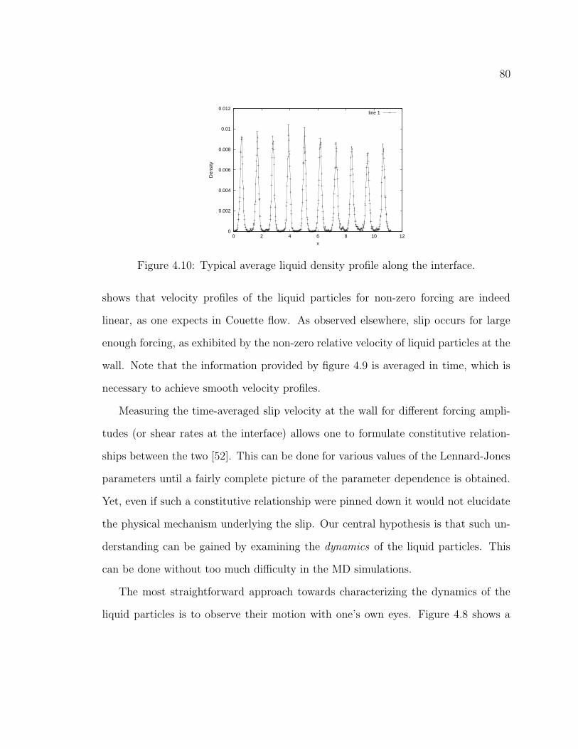
80

0

0.002

0.004

0.006

0.008

0.01

0.012

0 2 4 6 8 10 12

Den

sity

x

line 1

Figure 4.10: Typical average liquid density profile along the interface.

shows that velocity profiles of the liquid particles for non-zero forcing are indeed

linear, as one expects in Couette flow. As observed elsewhere, slip occurs for large

enough forcing, as exhibited by the non-zero relative velocity of liquid particles at the

wall. Note that the information provided by figure 4.9 is averaged in time, which is

necessary to achieve smooth velocity profiles.

Measuring the time-averaged slip velocity at the wall for different forcing ampli-

tudes (or shear rates at the interface) allows one to formulate constitutive relation-

ships between the two [52]. This can be done for various values of the Lennard-Jones

parameters until a fairly complete picture of the parameter dependence is obtained.

Yet, even if such a constitutive relationship were pinned down it would not elucidate

the physical mechanism underlying the slip. Our central hypothesis is that such un-

derstanding can be gained by examining the dynamics of the liquid particles. This

can be done without too much difficulty in the MD simulations.

The most straightforward approach towards characterizing the dynamics of the

liquid particles is to observe their motion with one’s own eyes. Figure 4.8 shows a

81

typical snapshot of the system for εlw

εll= σlw

σll= 1. In this case, in which the liquid-

liquid and solid-solid inter-particle spacings are identical the liquid particles nearest

the wall spend much of their time in the potential wells of the wall, although they

vibrate due to the non-zero temperature.

Consider a frame of reference moving with the wall. Thus, if there is no slip, the

liquid molecules adjacent to the wall would have zero velocity. We will assume that

a force is applied in the right-hand direction and so, relative to the molecules at the

wall, molecules in the bulk move to the left. By downstream we refer to motion in

the direction of the forcing, that is, to the right.

The effect of the motion of the liquid particles above the layer adjecent to the wall

is striking. From the point of view of a particular molecule, occasionally a molecule

will pass overhead with a horizontal velocity to the left, exerting a force sufficient to

dislodge the bound molecule. One of two events generically occurs in this case. The

dislodged molecule either migrates upwards away from the wall or it proceeds (to the

left) to the next potential well, thereby dislodging the liquid molecule residing there.

In the former case a potential well is left vacant. The downstream liquid particle

(in the sense of the forcing) feels a strong upstream force due to the sudden absence

of the repulsive force of its neighbor. It therefore jumps over the potential hump to

occupy the vacant well. This hole clearly propagates downstream as particles jump

one at a time to fill the vacancy. The propagation ends when a liquid molecule from

above migrates into the potential well, thus restoring the wall layer to an integer

value of ξ (defect-free state). Hole propagation can clearly be seen in the lower left

hand panel in figure 4.11, initiated by the dissapearance of the fourth particle from

the right, leading to the leftward motion of molecules 3, 2, and 1 respectively.

82

x

t

Figure 4.11: Typical particle trajectories for the layer of liquid at the interface. Bot-tom figures are blow-ups of the red boxes in the upper panels. Slip is indicated byleftward motion.

83

In the latter case the dislodging events also occur consecutively until an excess

particle migrates upwards and the integer value of ξ is restored. In this case the

propagation is upstream. Observation indicates that this scenario is less prevalent

than the propagation of holes. Note that upstream propagation of an excess particle

or downstream propagation of a hole both result in a net upstream transport of

particles. This is precisely what is meant by liquid slip. We have already seen in

much detail the effect of an excess particle or missing particle in a chain of particles

in the FK model. This type of defect motion seems to be an appropriate description

of the actual dynamical states arising in the MD simulations, which lead to net slip

on the average.

Important for the degree of slip in the scenario described above is the rate at

which particles leave and migrate to the interface. Indeed, it is this particle transport

perpendicular to the wall that both leads to the creation and anihilation of defects.

Figure 4.12 shows the rate of particle transport as a function of distance from the

wall. This function looks strikingly similar to the density profile perpendicular to the

wall, and in fact the particle transport dips down to very low values near the first

trough. This means that the spike in particle density near the wall (the first layer)

is comprised of particles which spend a considerable amount of time near the wall.

Occasionally particles leave or enter the first layer, but on short enough time scales

the particles can be reasonably modeled as a coherent chain.

84

0

0.1

0.2

0.3

0.4

0.5

0.6

0 1 2 3 4 5 6

Par

ticle

flux

y

Figure 4.12: Typical liquid density (line of x’s) and mass flux (dotted line) normal tothe interface.

85

4.9 The variable-density Frenkel-Kontorova Model

We have dwelt much on the dynamics of the FK model in sections 4.2 through 4.7. In

the last section we introduced some results from MD simulations and gave an anec-

dotal account of particle dynamics to motivate the usefulness of a FK-like model. We

noted that the vertical flux of liquid particles was important for determining the rates

of creation and anihilation of defects. In this section we propose a modified version

of the FK model in which the number of particles may change in time. This occurs

stochastically according to probabilities for seeding in or removing existing particles.

As we shall see, the most realistic choice is of probabilities which depend themselves

on the current number of particles 4 (nature hates a vacuum). We present a simple

theory for calculating the slip velocity in this model. We conclude by comparing these

results to those obtained in MD.

The variable-density Frenkel-Kontorova model (vdFK) is given by 4.2 with a rule

for determing how the number of particles N = N(x, t) should change in time and

space. We choose a probabilistic algorithm. A new particle is added or a particle is

taken away in a time unit dt with probability p+dt and p−dt respectively. In addition,

these probabilities have the form

p+ = p+ α[s− a]+ (4.62)

p− = p+ α[a− s]+ (4.63)

where a and s are the number of particles added and subtracted and [(·)]+ is the

4Thanks to Shreyas for immediately noticing this.

86

positive rectifying function which is positive for positive argument and zero otherwise.

The term proportional to α reflects the fact that the system prefers the defect-free

state a = s. We might also have chosen a ‘soft’ dependence on the number of defects

such as

p+ = pe−β[s−a]+ + (1 − e−β[s−a]+) (4.64)

p− = pe−β[a−s]+ + (1 − e−β[a−s]+) (4.65)

which varies continuously between p and 1 as a function of the number of defects.

The probability of having d defects as a function of time can be expressed as

p(d(t)) = p(|a(t) − s(t)| = d). The resulting probability density function pdf given

4.62 and 4.63 is discussed in the appendix C. In what follows we assume the form of

the pdf is known. The pdf itself can be generated numerically from MD simulations.

We furthermore need to decide where the liquid particles should be seeded in and

which ones should be removed. If an event occurs at time to then a particle is chosen

at random from the N(to) particles with probability 1N(to)

. If a particle is to be added,

it is placed, for simplicity, exactly between the selected particle i and particle i + 1.

Otherwise the selected particle is removed.

We summarize the model in non-dimensional form for clarity

xi = − sin xi + k4†4xi − ηxi + f,

N = N(t), (4.66)

and emphasize that the vdFK model is non-deterministic due to the fluctuations in

87

x

t

Figure 4.13: A qualitative comparison of liquid particle dynamics at the solid interfacein the MD simulations (left) and in the vdFK equation (right).

88

the density of particles. Nonetheless, given the results already obtained in previous

sections concerning the properties of defects in the FK model, we will be able to

predict the slip velocity in the vdFK model for certain parameter values.

We first consider the case of an initially integer-commensurate value of ξ. We note

that for p+ = p− = 0 the system exhibits no slip for f ≤ 1 and that a SN bifurcation

to bulk slip occurs at f = 1. In the case of n weakly interacting defects we have

determined that for f < fcr no slip occurs, while for fcr = EPN (fcr)λ

a SN bifurcation

to defect motion occurs. Furthermore, the defect velocity is given by vd(f, η) and the

total slip velocity is just < v >= n · vd.

A simple approximation of the slip velocity in 4.66 for weakly interacting defects

would then be

< v >= limT→∞

vd(f − fcr, η)

T

∫ T

0

dtd(t), (4.67)

which is just the velocity of a single defect times the average number of defects. We

note that the velocity of holes is in general different than that of extra particles, but

given the symmetry p+(a, s) = p−(s, a), it is clear there should be as many holes on

average as extra particles. Thus we can take vd(f, η) =vhole+vparticle

2in 4.67. Once vd

is known, 4.67 can be calculated numerically for any simulation. However, if the pdf

governing the evolution of N(t) is known, 4.67 can, in theory, be calculated explicitly.

We define the expected slip velocity

E(< v >) = limT→∞

vd(f − fcr, η)

T

∫ T

0

dtE(d(t)) (4.68)

89

Figure 4.14: Number of defects as a function of time for both zero and non-zero α.

where

E(d(t)) =∞∑

d=0

d · p(d(t)). (4.69)

Equations 4.67 and 4.68 makes use of the steady-state velocity of moving defects

in the FK model. When an extra particle is initially introduced, or one taken away,

there will be a transient response before the steady state value is reached. For large

enough particle fluxes, such steady state values may never be reached, i.e. before

a defect reaches its steady state velocity, it is perturbed or anihilated. In this case

equations 4.67 and 4.68 will break down and we must develop a theory of transients.

Dynamics in the vdFK equation

Here we take a closer look at the dynamics that arise in the vdFK model. We

remark first on the importance of the parameter α which determines how strongly

the system is attracted to the defect-free state. Figure 4.14 shows a sample time

90

series of the number of ‘defects’ d(t) for p = 0.1 and two different values of α. For

α = 0.0001 the value of d(t) is already drastically reduced. This is important for two

reasons. Firstly, it is what one sees in MD simulations and what one expects in a

real liquid; the interfacial liquid particles will always tend to their ‘ground’ state, the

most energetically preferred state. The particles constitute a driven system and thus

defects arise, but the system will continually seek to anneal itself. Secondly, in the

context of the vdFK model, large deviations in d(t) and therefore ξ would result in

jumps between qualitatively different types of behavior. If ξ varies only slightly, e.g.

deviates but little from an integer commensurate value, then the ensuing dynamics

can be described straightforwardly, e.g. as given by 4.67.

Consider figure 4.15. Left-hand figures show the velocity averaged over all particles

in the vdFK model and the number of particles as a function of time. The forcing is

f = 0.0, 0.6, 1.2 and increases from top to bottom, while the right hand figures show

individual events in greater detail.

With zero forcing (uppermost figures) the response of the system to the addition

or subtraction of a particle is complex. The effect on the average velocity of the

system can be discerned as a localized spike of either positive or negative amplitude.

A close-up view of such a spike in the velocity is shown on the right although much

more complex responses can be seen as well.

The change in velocity due to the introduction of defects in the driven system

(central panels) is much more straightforward. For nonzero values of d(t), the velocity

rapidly approaches a fixed value (although oscillations are, of course, present, as

the righthand figure shows). Furthermore, the more defects present, the larger the

velocity. In fact, it seems the effect of a defect is to cause a step of fixed amplitude in

91

Figure 4.15: Velocity averaged over all particles and number of particles as a functionof time in a small system. Here the system consists of 10 periods of the substrate withan initial condition of 10 particles, i.e. ξ = 1. This system size was chosen to comparewith MD simulations. The forcing increases from top to bottom, f = 0.0, 0.6, 1.2respectively. Other parameter values are p = 0.001, α = 0.0001, η = 2 and k = 1.

92

Figure 4.16: Left: The addition of a defect (x = 18) reduces the effective potentialbarrier and the resultant motion is smoother. Parameters are f = 1.2, η = 2.0,k = 1.0, p = 0.001 and α = 0.001. Right: Close-up of defect motion. The defectmotion can be discerned as a wave traveling from right to left after the addition of anexcess particle. Parameters are f = 0.8, η = 2.0, k = 0.1, p = 0.001 and α = 0.001.

the velocity. This is precisely the meaning of 4.67 and we expect it to be an accurate

measure of slip in this regime.

For f = 1.2, i.e. beyond the SN bifurcation to bulk slip, two very distinct regimes

can be seen, depending of the value of d(t). For d(t) = 0 the chain of particles slides

over the substrate as expected, resulting in a mean slip velocity with large oscillations

(the oscillations have the largest amplitude nearest the SN, of course). Introduction of

a defect pushes the system far from the critical slowing regime near the SN bifurcation

and the motion is nearly free of oscillation (see lefthand panel of figure 4.16).

Space-time diagrams of the particle trajectories are compared to the corresponding

averaged velocities in figure 4.17. The probability p = 0.0001, 0.001, 0.01 increases

from top to bottom. The topmost panel clearly shows how slip is initiated if a particle

is removed (particle removed at x ∼ 6 and t ∼ 600). The neighboring particles feel

93

a sudden change in force and no longer sit in an equilibrium state. The upstream

particle is pulled into the vacant well and the hole thus propagates upstream. Removal

of a second particle (x ∼ 45 and t ∼ 850) increases the slip additively through the

same mechanism.

The central panel illustrates the effect of introducing an extra particle, both in

the case where this restores the defect-free state of the system d(t) → 0 and in the

case where a defect is created. Note at t = 700, x ∼ 5 and t = 850, x ∼ 38 the

introduction of a particle halts the propagation of defects and leads to zero slip, while

at t = 950, x ∼ 22 a defect is introduced and motion once again begins. Dynamics in

the lower panel appear quite disordered due to the high flux of particles. Nonetheless,

the stereotypical events described above can still be clearly discerned as the building

blocks of the resultant slip.

Figure 4.18 shows both slip velocties and particle trajectories for the case of weak

inter-particle coupling (k = 0.1). The dynamics are qualitatively similar to the case

described above, although of note are the large oscillations in the velocity of prop-

agating defects. This comes as no surprise. The Peierls-Nabarro potential increases

with decreasing inter-particle coupling strength. In figure 4.18 we are just past the

SN bifurcation to defect motion (not to be confused with the SN bifurcation to bulk

motion), which naturally leads to large oscillations in the propagation velocity.

Finally, in figure 4.19 we see that the prediction from 4.67 (red lines) captures

the degree of slip well. One consequence of this is that for large enough inter-particle

coupling (e.g. k = 1 here) the slip velocity increases almost linearly in the forcing

(see figure 4.4, inset). This leads to a constant slip length as seen in the righthand

panel of figure 4.19. Past the SN bifurcation point to bulk slip the curves all converge.

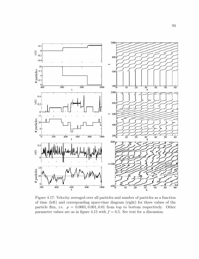
94

Figure 4.17: Velocity averaged over all particles and number of particles as a functionof time (left) and corresponding space-time diagram (right) for three values of theparticle flux, i.e. p = 0.0001, 0.001, 0.01 from top to bottom respectively. Otherparameter values are as in figure 4.15 with f = 0.5. See text for a discussion.

95

Figure 4.18: Case of weakly coupled particles, i.e. kh

small. Left: Velocity averagedover all particles and number of particles as a function of time. Right: Space-timediagram of particle trajectories. Parameters are f = 0.8,η = 2.0,α = 0.001,k = 0.1and p = 0.001 (top), p = 0.002 (bottom).

However, for large enough flux the bifurcation itself is smeared out. The agreement

between theory and simulation of the vdFK equation appears to be slightly less robust

for weak coupling, perhaps due to the interaction of oscillatory modes generated by

the defect motion near the SN bifurcation to defect-slip.

Figure 4.19 shows slip lengths of a fraction of a particle diameter, which is rather

small. Reducing the effective friction between the liquid particles and the wall con-

siderably increases slip length. Consider figure 4.20 where ηfs = 0.1, one tenth the

96

0 0.5 1 1.5f

0

0.1

0.2

0.3

0.4

0.5

0.6<

v>

p=0.001p=0.0005p=0.0001

0.1 1γ

0

0.1

0.2

0.3

0.4

0.5

0.6

Ls

p=0.001p=0.0001p=0.0005

.

0 0.5 1 1.5f

0

0.1

0.2

0.3

0.4

<v>

p=0.0001p=0.0005p=0.001p=0.002

0.1 1γ

0

0.1

0.2

0.3

0.4

0.5

Ls

p=0.0001p=0.0005p=0.001p=0.002

.

Figure 4.19: Slip velocity and slip length as a function of forcing for various valuesof p (see legend of each figure) with α = 0.001 and η = 2. The equilibrium value ofξ is here 1. Top panels are for k = 1, bottom panels for k = 0.1. Red lines are theprediction from 4.67, symbols are numerical data and black lines are meant only asguides to the eye. Slip length is shown on lin-log scale to facilitate comparison withpublished data.

previous value. This leads to roughly a ten-fold increase in the slip length. Larger

slip lengths can be obtained by further reducing the effective friction. Also note that

4.67 captures the degree of slip well (see red lines in figure 4.20) with the exception of

p = 0.01, for which the particle flux is too high to consider the defects independent.

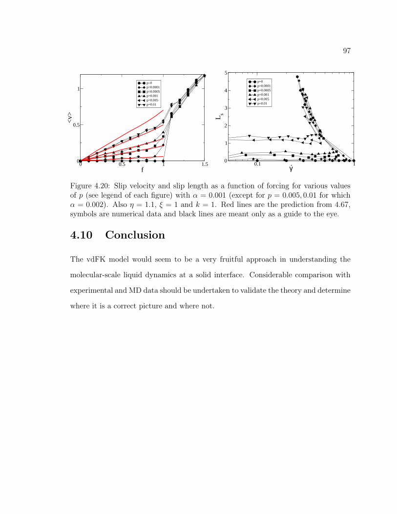
97

0 0.5 1 1.5f

0

0.5

1

<v>

p=0p=0.0001p=0.0005p=0.001p=0.005p=0.01

0.1 1γ

0

1

2

3

4

5

Ls

p=0p=0.0001p=0.0005p=0.001p=0.005p=0.01

.

Figure 4.20: Slip velocity and slip length as a function of forcing for various valuesof p (see legend of each figure) with α = 0.001 (except for p = 0.005, 0.01 for whichα = 0.002). Also η = 1.1, ξ = 1 and k = 1. Red lines are the prediction from 4.67,symbols are numerical data and black lines are meant only as a guide to the eye.

4.10 Conclusion

The vdFK model would seem to be a very fruitful approach in understanding the

molecular-scale liquid dynamics at a solid interface. Considerable comparison with

experimental and MD data should be undertaken to validate the theory and determine

where it is a correct picture and where not.

Chapter 5

A Novel Interaction of Shaeffer

Collateral and Temporo-Ammonic

Inputs in a Model of a CA1

Pyramidal Cell

5.1 The SC and TA pathways

The hippocampus forms part of the primitive cortex of the brain and is involved in

the formation of certain types of memory, expecially spatially-related memory [73].

The architecture of the hippocampus, as well as the diversity of cell types and their

electrophysiological properties, have been intensively studied both in vitro and in

vivo, especially in the rat [74].

According to the classical picture of hippocampal organization, the hippocampus

98

99

Figure 5.1: The rat hippocampus. The ‘tri-synaptic’ loop is highlighted on the right,including the two main excitatory inputs to CA1 pyramidal cells: the Temporo-Ammonic (TA) pathway (pink) and the Schaeffer Collaterals (SC) (green)

communicates with the cerebral cortex via the so-called ‘trisynaptic circuit’ (see fig-

ure 5.1). Input from the entorhinal cortex enters the hippocampus via the perforant

pathway, which consists of two distinct sets of axons, one emanating from layer II

and the other from layer III. Layer III axons (Temporo-Ammonic pathway (TA))

project directly to distal CA1 pyramidal cell dendrites in stratum lacunosum molec-

ulare (SLM). The axons from layer II enter the dentate gyrus where they synapse

onto dentate granule cells. Mossy fibers from the granule cells project to the CA3

region of the hippocampus, where a high degree of collateralization implies a highly

nonlinear feedback process. CA3 pyramidal cell axons, called the Schaeffer Collater-

als (SC), synapse onto apical dendrites of CA1 pyramidal cells in stratum radiatum

(SR). Finally, CA1 pyramidal cells project back to the deeper layers of the entorhinal

100

cortex, finishing the ‘loop’. The very small degree of collateralization in the CA1 re-

gion implies that the input-output relationship of CA1 pyramidal cells may to some

extent be understood at a single-cell level. This neglects the very complex network

of hippocampal interneurons [75].

The classical notion of the trisynaptic circuit is an oversimplification and many

other projections to, from and within the hippocampus are known to exist [74].

Nonetheless, it is accurate to consider the SC and TA pathways to be the main

excitatory inputs to CA1 pyramidal cells. Dynamical differences between the TA and

SC pathways have very recently been investigated in vivo in guinea pigs [76] through

extracellular recordings. The results show that the two pathways are selectively acti-

vated and thus dynamically distinct.

In this chapter we study the dynamical interaction of excitatory inputs from TA

and SC pathways at the level of a single CA1 pyramidal cell through extensive simula-

tions using NEURON. Our main result is a novel mechanism of coincidence detection

involving the forward propagation of dendritic sodium-spikes (Na-spikes). Na-spikes

generated in the apical tuft via the TA input, which generically do not cause somatic

APs, may be ‘gated’ through to the soma if the main apical dendrite is sufficiently

depolarized by SC input. The inputs must consequently also be sufficiently syn-

chronous.

101

5.2 A model of a CA1 Pyramidal cell in NEURON

Three different pyramidal cell morphologies were used in simulations. 1 All three

correspond to CA1 pyramidal cells of the rat hippocampus, reconstructed with the

neurolucida microscope and converted into NEURON format. The three cells are

referred to as ri04, ri05 and ri06 and are shown in figures 5.2, 5.3 and 5.4 respectively.

Morphology can strongly affect the electrophysiological properties of neurons, includ-

ing backpropagation of somatic APs and forward propagation of dendritic spikes [77].

We thus test three cells in order to determine to what extent our results are robust

to morphological perturbations. The NEURON code for cell ri06, with the exception

of the synapses, is the same as that used in [78].

The morphological data is in the form of a set of cartesian coordinates and asso-

ciated diameters. NEURON then resconstructs the cell by joining together cylinders

with given diameters (note the varying line thickness in figure 5.2, which reflects the

recorded diameter, for example). The CA1 pyramidal-cell morphology can be sub-

divided naturally into distinct sections, both according to the nature of the inputs

received as well as the electrophysiological properties of the neuron itself. In the

present study, we distinguish between the following regions: soma, axon, basal den-

drites, apical dendrites, and apical tuft. In addition, we also distinguish between the

main apical dendrite and the oblique apical dendrites, which differ in the density of

synaptic connections.

Table 5.1 shows the values of some passive cell properties. These values hold

for all cell sections and all three cells unless otherwise noted. The variables are

1Morphological data for all three cells were obtained from the lab of Nelson Spruston.

102

Cm (µF/cm2) Cmy (µF/cm2) Rm (Ω · cm2) Ra (Ω · cm) Vleak (mV )0.75 0.04 40000 200 -66

Table 5.1: Passive cell properties.

membrane capacitance (Cm), capacitance at the myelinated internodes of the axon

(Cmy), membrane resistance (Rm), axial resistance (Ra) and a leak reversal-potential

(Vleak). The membrane capacitance also varies as a function of distance from the

soma. The presence of spines in the more distal portion of the apical dendrites is

modeled as an increased capacitance (by a factor of two) for all apical dendrites at a

distance greater than 300µm.

The ability of the cell to generate action potentials, as well as the active prop-

erties of the dendrites, depend on the presence of voltage-dependent ionic channels.

The model used in this work includes four distinct currents: an inactivating sodium

current, a delayed-rectifying potassium current and two additional A-type potassium

currents, which activate at relatively low potentials. The A-currents activate and inac-

tivate rapidly. NEURON models the ionic currents by solving the voltage-dependent

differential equations for the fraction of open channels for each ionic species. The

contribution, for example, of the sodium current at a given point in the cell is

INa = geff(V − ENa+) (5.1)

geff = gNam3h (5.2)

where the kinetic variables m and h, representing activation and inactivation respec-

tively, are modeled via first-order equations with voltage-dependent time-constants

and asymptotic values.

103

soma/basal Na+ K+dr A-type K+ (prox.)

g (1/Ω · cm2) 0.048 0.040 0.048E (mV ) 55 -90 -90axongnode 30.0 0.040 0.0096ginternode 0.048 0.040 0.0096E 55 -90 -90apicalg ≥ 0.048 0.040 ≥ 0.048E 55 -90 -90

Table 5.2: Active cell properties by section. The parameters gnode and ginternode arethe conductances at and between the nodes of Ranvier respectively.

The values of the maximal conductances for each type of channel vary across

the cell. Table 5.2 shows a characterization of the ionic channels broken down by

section. Note, in particular, that the sodium and A-type potassium conductances vary

spatially in the apical dendrites. Gradients in channel densities have been verified in

experiment and used in simulations elsewhere previously [79]. Specifically, the sodium

conductance varies as a function of the distance x from the soma as

gNa(x) = gNa(1 + αNa · x) x < x∗Na,

gNa(x) = gNa(1 + αNa · x∗Na) x > x∗Na, (5.3)

(5.4)

where α takes the value of 0 or 0.001, the latter being what we refer to as the ‘strongly

back-propagating’ case. Unless noted otherwise, the default value of α will be 0. The

104

value of x∗Na is 500µm. The potassium conductances vary as

gK(x) = gK(1 + βp · x) x < x,

gK(x) = gK(1 + βd · x) x < x < x∗K ,

gK(x) = gK(1 + βd · x∗K) x > x∗K , (5.5)

where βp = βd = 0.01 (but can, in general, be different from one another) are the

slopes of the conductance gradient for the proximal and distal potassium currents

respectively. The values of x and x∗K are 100µm and 500µm respectively. These

values correspond to those used in [79].

In addition to the passive and active properties described above, we place both

excitatory (AMPA) and inhibitory (GABA) synapses on the cell. Experimental mea-

surement of the density of synapses in CA1 pyramidal cells provides the estimates

shown in table 5.3 [80]. Total numbers of synapses are around 30,000 of each type

for each cell. Note that sub-sections of the apical dendrites labeled lower, mid-

and upper correspond roughly to the first 150µm, next 150µm and remaining dis-

tance (around 150µm) to the apical tuft respectively. Both excitatory and inhibitory

synapses are modeled as double-exponential synapses (point-process Exp2Syn with

NetCon in NEURON). Synaptic properties are given in table 5.4. Note that the max-

imum synaptic conductance is 100 pico-Siemens (pS) in each case. Empirical data

indicate that activation of a synapse recruits between 10 and 100 channels, each of

which contribute around 10 pS conductance change with an average around 35. Thus

our choice is at the lower end of synaptic strength. As such, the activation of 100

synapses in this work may be equivalent to the activation of anywhere between 10

105

Figure 5.2: Pyramidal cell ri04. Axes indicate distance in microns from the soma.

106

Figure 5.3: Pyramidal cell ri05. Axes indicate distance in microns from the soma.

107

Figure 5.4: Pyramidal cell ri06. Axes indicate distance in microns from the soma.

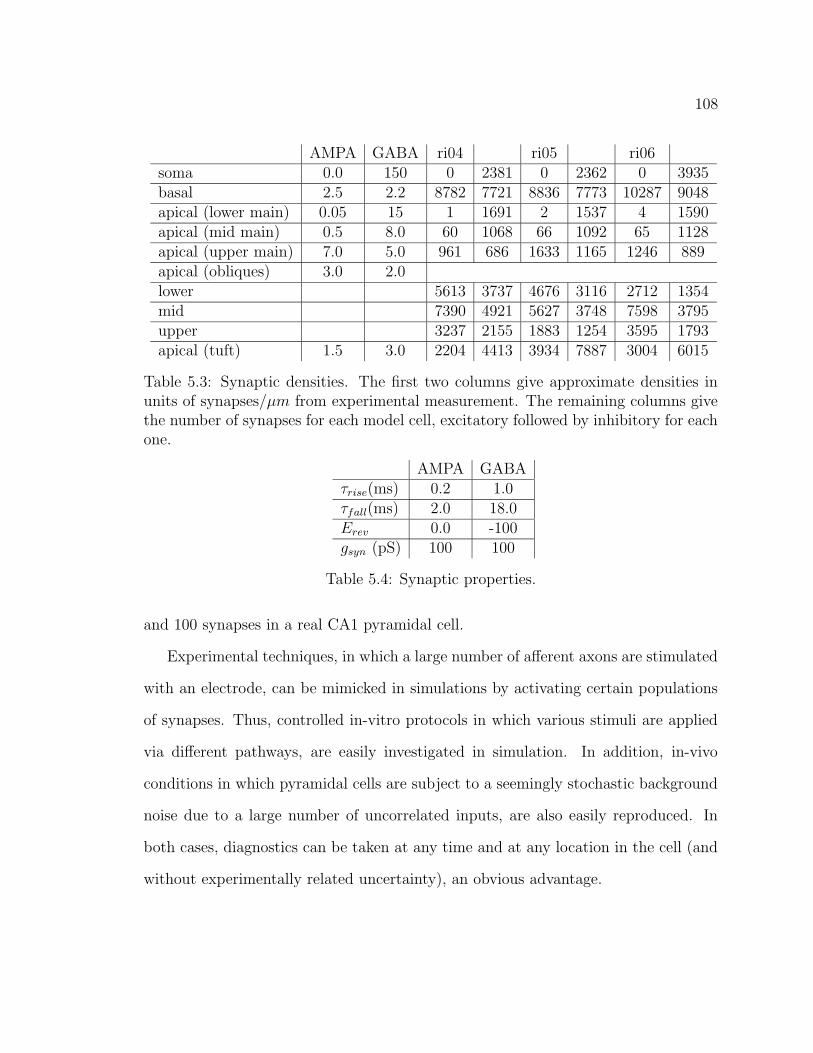
108

AMPA GABA ri04 ri05 ri06soma 0.0 150 0 2381 0 2362 0 3935basal 2.5 2.2 8782 7721 8836 7773 10287 9048apical (lower main) 0.05 15 1 1691 2 1537 4 1590apical (mid main) 0.5 8.0 60 1068 66 1092 65 1128apical (upper main) 7.0 5.0 961 686 1633 1165 1246 889apical (obliques) 3.0 2.0lower 5613 3737 4676 3116 2712 1354mid 7390 4921 5627 3748 7598 3795upper 3237 2155 1883 1254 3595 1793apical (tuft) 1.5 3.0 2204 4413 3934 7887 3004 6015

Table 5.3: Synaptic densities. The first two columns give approximate densities inunits of synapses/µm from experimental measurement. The remaining columns givethe number of synapses for each model cell, excitatory followed by inhibitory for eachone.

AMPA GABAτrise(ms) 0.2 1.0τfall(ms) 2.0 18.0Erev 0.0 -100gsyn (pS) 100 100

Table 5.4: Synaptic properties.

and 100 synapses in a real CA1 pyramidal cell.

Experimental techniques, in which a large number of afferent axons are stimulated

with an electrode, can be mimicked in simulations by activating certain populations

of synapses. Thus, controlled in-vitro protocols in which various stimuli are applied

via different pathways, are easily investigated in simulation. In addition, in-vivo

conditions in which pyramidal cells are subject to a seemingly stochastic background

noise due to a large number of uncorrelated inputs, are also easily reproduced. In

both cases, diagnostics can be taken at any time and at any location in the cell (and

without experimentally related uncertainty), an obvious advantage.

109

Figure 5.5: Part of the graphical user interface (gui) controlling the stimulus proper-ties.

Figure 5.5 shows part of the graphical user interface (gui) designed to facilitate the

control of the synaptic stimulus (here for AMPA). The cell is divided into 5 sections for

which the percentage of active synapses can be chosen. In figure 5.5, seven percent of

the synapses located in the upper apical dendrites (including oblique apical dendrites)

are active. Once a section is activated, the stimulus properties can be set, including

the start time of stimulus, average inter-spike-interval (ISI), average number of spikes

and ‘degree of stochasticity’. This last parameter interpolates between a periodic and

a Poisson train of EPSCs as it varies from 0 to 1.

110

5.3 Response to single inputs

In order to investigate the response of our model pyramidal cells to paired SC and TA

inputs, we must first characterize their dynamics in response to single inputs. CA1

pyramidal cells have a very extensive dendritic arbor, penetrating into stratum oriens

and the alveus (basal dendrites) as well as all the way through stratum radiatum

(SR) and into stratum lacunosum moleculare (SLM). Distal inputs from the SLM

may be as far away from the cell body as 700µm. Passive attenuation will make such

an input much less effective in eliciting an action potential than an identical input

nearer the soma. However, active dendritic properties including the generation of

dendritic spikes, may complicate this picture and lead to the cell acting as a highly

non-linear integrator.

Figure 5.6 shows the average peak depolarization (100 trials) at three points in

the cell ri04 for four different stimuli. The stimuli are to the lower-apical, mid-

apical, upper-apical and apical tuft, left to right, top to bottom respectively. The

three ‘recording electrodes’ are indicated by black circles (soma), red squares (main-

apical dendrite ∼ 250µm) and blue diamonds (apical tuft ∼ 700µm). The standard

deviation of the 100 trials is given by error bars.

It is clear that the likelihood of generating an action potential (AP) decreases as

the locus of the stimulation moves further and further from the soma. Consider, for

example, that activation of a mere 2% of the synapses in the lower apical region (about

112 synapses from 5.3) is sufficient to very reliably elicit APs, while stimulation of

the mid-apical region requires 3% (240 synapses) and this increases to 11% for upper-

apical stimulation (over 400 synapses). Finally, stimulation of the tuft never causes

111

0 2 4 6 8 10% synapses stimulated

0

50

100

peak

dep

. (m

V)

lower-apical stimulationcell -04

0 2 4 6 8 10% synapses

0

50

100

peak

dep

. (m

V)

mid-apical stimulationcell -04

0 5 10 15% synapses

0

50

100

peak

dep

. (m

V)

upper-apical stimulationcell -04

0 2 4 6 8 10% synapses

0

10

20

30

40

50

60

70

peak

dep

. (m

V)

tuft stimulationcell -04

Figure 5.6: Response properties of the cell ri04. Voltages were recorded from thesoma (black circles), the main apical dendrite (red squares) and the apical tuft (bluediamonds).

112

an AP. Note that the large depolarization in the main-apical dendrite (red squares)

whenever APs occur is the signature of reliable backpropagation of the AP. That is,

whenever an AP occurs in the axon, it not only travels down the axon itself, but also

propagates backwards into the dendritic arbor via the activation of Na channels in

the membrane of the dendrites. This process is ubiquitous in pyramidal cells of both

the hippocampus and the cerebral cortex [81].

Interestingly, while for sufficiently small stimuli in the tuft (lower right-hand panel)

the resulting local integration of EPSPs appears to be more or less linear as a function

of stimulus intensity (and thus passive), larger stimuli (> 5%) readily elicit variable-

amplitude, nonlinear events. Thus dendritic Na-spikes occur locally in the tuft but

fail to initiate an AP at the soma. In fact, the attenuation of the dendritic spikes

is so great that their influence is hardly felt at the soma (see black circles in same

panel).

It was shown in [78] that the experimentally observed dichotomy in the efficacy

of backpropagation in CA1 pyramidal cells can be explained by a slight gradient in

the density of Na channels in the apical dendrites. Those neurons which exhibit this

positive gradient in the channel density are referred to as strong-backpropagating

(SBP) neurons. Figure 5.7 shows data analogous to that in figure 5.6 for the SBP

case. Note the two principal differences. Firstly, whenever an AP occurs, the back-

propagation consistently reaches the apical tuft resulting in a large depolarization

(blue diamonds). Secondly, Na-spikes generated locally in the tuft now sometimes do

elicit somatic APs (lower right-hand panel).

Figures 5.8 through 5.11 show analogous data for the other two cells, both for

the standard and SBP cases. Note the qualitative similarity for all three cells despite

113

0 2 4 6 8 10% synapses stimulated

0

50

100

peak

dep

. (m

V)

lower apical (SBP)cell -04

0 2 4 6 8 10% synapses

0

50

100

peak

dep

. (m

V)

mid-apical stimulation (SBP)cell -04

0 2 4 6 8 10% synapses

0

50

100

peak

dep

. (m

V)

upper-apical stimulation (SBP)cell -04

0 2 4 6 8 10% synapses

0

50

100

peak

dep

. (m

V)

tuft stimulation (SBP)cell -04

Figure 5.7: Response properties of the cell ri04 for the strongly back-propagatingcase.

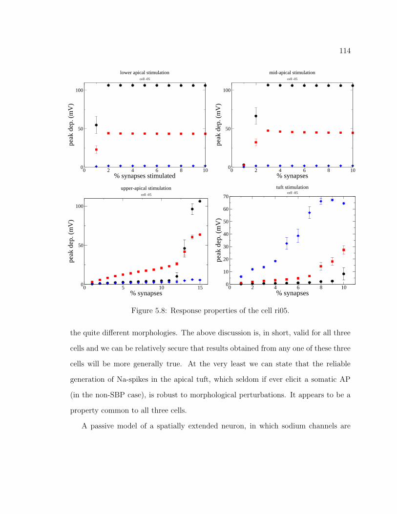
114

0 2 4 6 8 10% synapses stimulated

0

50

100

peak

dep

. (m

V)

lower apical stimulationcell -05

0 2 4 6 8 10% synapses

0

50

100

peak

dep

. (m

V)

mid-apical stimulationcell -05

0 5 10 15% synapses

0

50

100

peak

dep

. (m

V)

upper-apical stimulationcell -05

0 2 4 6 8 10% synapses

0

10

20

30

40

50

60

70

peak

dep

. (m

V)

tuft stimulationcell -05

Figure 5.8: Response properties of the cell ri05.

the quite different morphologies. The above discussion is, in short, valid for all three

cells and we can be relatively secure that results obtained from any one of these three

cells will be more generally true. At the very least we can state that the reliable

generation of Na-spikes in the apical tuft, which seldom if ever elicit a somatic AP

(in the non-SBP case), is robust to morphological perturbations. It appears to be a

property common to all three cells.

A passive model of a spatially extended neuron, in which sodium channels are

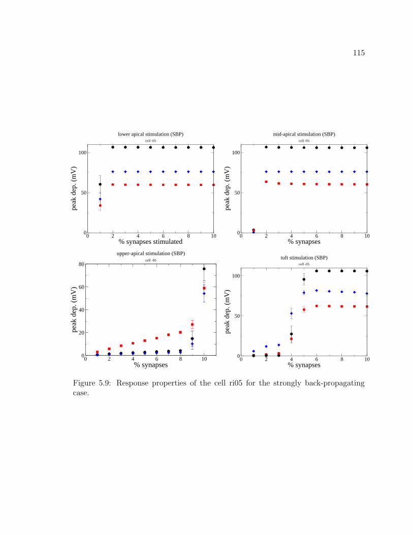
115

0 2 4 6 8 10% synapses stimulated

0

50

100

peak

dep

. (m

V)

lower apical stimulation (SBP)cell -05

0 2 4 6 8 10% synapses

0

50

100

peak

dep

. (m

V)

mid-apical stimulation (SBP)cell -05

0 2 4 6 8 10% synapses

0

20

40

60

80

peak

dep

. (m

V)

upper-apical stimulation (SBP)cell -05

0 2 4 6 8 10% synapses

0

50

100

peak

dep

. (m

V)

tuft stimulation (SBP)cell -05

Figure 5.9: Response properties of the cell ri05 for the strongly back-propagatingcase.

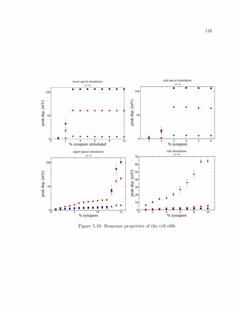
116

0 2 4 6 8 10% synapses stimulated

0

50

100

peak

dep

. (m

V)

lower apical stimulationcell -06

1 2 3 4 5 6% synapses

0

50

100

peak

dep

. (m

V)

mid-apical stimulationcell -06

0 5 10 15% synapses

0

50

100

peak

dep

. (m

V)

upper-apical stimulationcell -06

0 2 4 6 8 10% synapses

0

10

20

30

40

50

60

70

peak

dep

. (m

V)

tuft stimulationcell -06

Figure 5.10: Response properties of the cell ri06.

117

0 2 4 6 8 10% synapses

0

50

100

peak

dep

. (m

V)

lower apical stimulation (SBP)cell -06

2 4 6 8 10% synapses

0

50

100

peak

dep

. (m

V)

midapical stimulation (SBP)cell -06

0 2 4 6 8 10% synapses

0

50

100

peak

dep

. (m

V)

upper apical stimulation (SBP)cell -06

0 2 4 6 8 10% synapses

0

50

100

peak

dep

. (m

V)

tuft stimulation (SBP)cell -06

Figure 5.11: Response properties of the cell ri06 for the strongly back-propagatingcase.

118

removed from the dendrites (but not the soma or axon), would predict that more

distant stimuli would be less likely to elicit a somatic AP than a proximal one of

the same amplitude. The further away an EPSP occurs from the soma, the more

attenuation there will be at the soma and thus a greater absolute stimulus intensity

is needed for an AP. This notion is consistent with much of the data seen in figures

5.6 through 5.11. However, a close look at the initial site of spike generation reveals

that the picture of passive attenuation (diffusion) and integration is not sufficient to

understand the data.

Figure 5.12 shows the timing difference between the time of peak depolarization

measured both at the soma and along the main-apical dendrite as a function of stim-

ulus intensity for four different stimuli (lower-, mid- and upper apical and tuft). Data

are shown only for those trials where an AP occured. Consider the case where this

difference is negative (t(AP)-t(spike)< 0). This means the time of the peak depolar-

ization at the soma (due to the AP) occurs before the time of the peak depolarization

in the dendrite (due to the backpropagating AP). The AP thus clearly occured first

in the soma and propagated backwards. In the opposite case a spike must have been

generated in the dendrite first and propagated to the soma, thereby eliciting a somatic

spike. Where the timing difference is exactly zero both a somatic AP and a dendritic

spike occured simultaneously!

Consider cell ri06 (lower left-hand panel). A proximal stimulus (lower-apical, black

circles) always results in a somatic AP first. This is consistent with the notion that

very proximal EPSPs diffuse without appreciable attenuation to the soma. Activating

synapses in the mid-apical region (red squares) can cause APs both through passive

diffusion and the propagation of dendritic spikes as this data straddles the line of

119

0 5 10 15% synapses stimulated

-0.5

0

0.5

1

t(A

P)-t

(spi

ke)

cell ri04

0 2 4 6 8 10 12% synapses stimulated

-0.5

0

0.5

1

t(A

P)-t

(spi

ke)

SBPcell ri04

0 5 10 15% synapses stimulated

-0.5

0

0.5

t(A

P)-t

(spi

ke)

cell -05

0 2 4 6 8 10% synapses stimulated

-0.5

0

0.5t(

AP)

-t(s

pike

)

SBPcell -05

0 5 10 15% synapses stimulated

-1

-0.8

-0.6

-0.4

-0.2

0

0.2

0.4

0.6

0.8

1

t(A

P)-t

(spi

ke)

cell -06

0 2 4 6 8 10 12% synapses

-1

-0.8

-0.6

-0.4

-0.2

0

0.2

0.4

0.6

0.8

1

t(A

P)-t

(spi

ke)

SBPcell -06

Figure 5.12: Data showing the dichotomy of action potential generation via passiveintegration and forward propagation of dendritic spikes. A negative timing-differenceindicates that an AP was generated first, while a positive difference means a dendriticspike propagated to the soma and caused an AP. Colors correspond to the region ofthe apical dendritic tree to which the stimulus was applied: lower apicals (black),mid-apicals (red), upper apicals (green) and tuft (blue).

120

zero timing difference. Finally, a more distal stimulus (upper-apical) will always

cause denditic spikes first. Intracellular recordings from CA1 pyramidal cells in vitro

have revealed similar qualitative behavior in real cells [82].

5.4 Paired SC and TA inputs

We have now laid the groundwork for an investigation of the interaction between

inputs via the two principal excitatory pathways to CA1 pyramidal cells. In particu-

lar, we have examined the response of three morphologically distinct pyramidal cells

to stimuli focused at different points along the apical dendritic tree. We have seen

that the distal-most inputs, those which are reasonably interpreted as occuring within

SLM and thus from the TA pathway, reliably cause local Na-spikes, which however

fail to significantly influence the potential at the soma. This is in stark constrast to

a stimulus via the SC, which may cause action potentials through passive diffusion

of EPSPs or propagation of dendritic spikes.

What is the role of the TA input if it is unlikely to affect the soma? How does

the cell make use of the information it receives from these two pathways? In other

words what is the input-output relationship? It has recently been documented ex-

perimentally that combining these two stimuli results in an enhanced efficacy of AP

generation [83], but the mechanism remains unclear. It seems logical that two sub-

threshold stimuli may summate to provide sufficient depolarization at the soma for

AP generation. Nevertheless we show in this section that an active, highly non-linear

process is much more likely behind this increased efficacy. We compare simulations

of a passive model in which summating inputs only marginally improve the likelihood

121

of AP generation, with the above-studied active model where a very significant in-

crease in AP generation is obtained by combining two subthreshold inputs. In this

paradigm, a small, subthreshold depolarization via the SC is sufficient to ‘gate’ TA-

generated dendritic Na-spikes in the tuft, allowing them to propagate to the soma

thereby eliciting a somatic AP. The efficacy of the gating is furthermore dependent

on the relative timing of the two inputs.

In order to differentiate between those cell responses that are due to passive prop-

erties from those that are a consequence of active (voltage-dependent) dendritic cur-

rents, we remove the Na channels from the dendrites of our simulation of cell ri06.

Figure 5.13 shows data from representative trials in such a passive model, both for

SC and TA inputs. The upper panels display the maximum voltage during each run

as a function of distance x from the soma, while the bottom panels show traces of

voltage as a function of time. Note the almost complete absence of backpropagation

of AP’s for the SC input.

Figure 5.14 shows analogous data for the active case (with Na channels intact in

the dendrites). Here, for sufficiently large TA stimuli dendritic spikes are generated,

which however do not propagate to the soma.

We now investigate the effect of pairing syncronous SC and TA inputs, both for

the active and passive cases. Here we take a fixed TA stimulus (8%) while varying the

SC stimulus intensity. Figure 5.15 shows data from the paired (simultaneous inputs)

and unpaired protocols, with the active case in red and the passive case in black.

Plotted is the probability of a somatic AP (100 trials).

While it is not at all surprising that a greater stimulus intensity is needed to

generate AP’s in the passive case, it is striking that the likelihood of AP generation

122

Figure 5.13: Response of cell ri06 to SC and TA inputs in a passive model.

123

Figure 5.14: Response of cell ri06 to SC and TA inputs in an active model.

124

0 10 20 30 40% synapses (SC)

0

0.2

0.4

0.6

0.8

1p(

AP)

unpaired (Na)unpaired (no Na)paired (no Na)paired (Na)

-20 -10 0 10 20SC-TA

0

0.2

0.4

0.6

0.8

1

p(A

P)

SC 6%SC 8%

Figure 5.15: Response of cell ri06 to paired inputs. Left: Shift in the probability ofeliciting an action potential due to pairing the inputs. Note the considerable shiftin the active case in constrast to the passive case. Right: Probability of eliciting anaction potential as a function of the timing difference in ms between the two stimuli.The function is more or less peaked around the synchronous-pairing protocol.

is nearly unaffected by pairing the stimuli in the passive case, while the curve is

significantly shifted to the left in the active case. Note the greater than 50% reduction

in the threshold for AP generation in the active case. Comparison with the passive

case clearly shows this is not due to linear summation of the inputs.

Figure 5.17 provides an illustration of the mechanism underlying the increased

efficacy of AP generation for paired SC-TA inputs. The traces in the top two panels

correspond to the recording set-up shown in figure 5.16. This particular arrangement

was chosen to maximize the resolution around the primary apical bifurcation, essen-

tially the ‘gateway’ between the apical tuft and the main apical dendrite. Thus we

observe the voltage just above, just below and right at the bifurcation as well as in

the tuft, along the main apical dendrite and at the soma.

Consider the left-hand side of figure 5.17, for which the TA and SC stimuli are

125

Figure 5.16: The recording configuration for results shown in figure 5.17.

8% and 6.5% respectively. The second through fourth traces (at the bifurcation)

clearly show a depolarization beginning at 1ms atop of which there is even a small

active event (see bottom three traces, a blow-up). This depolarization is, however,

independent of the TA-driven Na-spike in the tuft. In fact, an artifact of the Na-spike

is visible in the second trace (see top trace of bottom panel) although it occurs several

ms after the intial, presumably SC-dependent depolarization. The amplitude of the

TA-driven spike thus attenuates considerably, and the SC stimulus is not sufficient

to elicit a somatic AP.

The right-hand side of figure 5.17 is for an identical simulation with a change only

in the amplitude of the SC stimulus (now 6.6%). The SC stimulus is now sufficiently

large to ‘gate’ the Na-spike through the primary apical bifurcation and to the soma.

Specifically, the small-amplitude remnant of the Na-spike in the second trace of the

126

-80-60-40-20

0

-80

-60

-40

-80

-60

-40

-80

-60

-40

-60

-40

0 5 10 15ms

-60

-40

-80-60-40-20

0

-80-60-40-20

-80-60-40-20

0

-80-60-40-20

0

-80-60-40-20

0

0 5 10 15ms

-80-60-40-20

02040

-75

-70

-65

-60

-55

-50

-70

-60

-50

-40

0 5 10 15ms

-75

-70

-65

-60

-55

-50

-80-70-60-50-40-30-20

-80

-60

-40

-20

0

0 5 10 15ms

-80

-60

-40

-20

0

Figure 5.17: Respresentative traces of voltage vs. time from a paired-input protocolwith a recording set-up as shown in figure 5.16. See text for details.

127

left-hand panel is now a large amplitude spike. Effective propagation of the TA-

induced Na-spikes is thus a threshold phenomenon, requiring sufficient depolarization

via SC inputs.

The relative timing of the two inputs strongly affects the efficacy of AP generation,

as shown in figure 5.15. The inputs must be sufficiently synchronous in order for the

Na-spikes to be gated. Two values of SC stimulus intensity are shown. Note that

increasing the SC stimulus intensity in this range significantly improves the likelihood

of eliciting an AP without resulting in a laxer criterion for synchronous inputs (the

width of the distribution increases only marginally). This is most likely due to the

presence of the A-type potassium currentsKA, which rapidly activate given a sufficient

depolarization, thereby shunting it out unless overwhelmed by a strong regenerative

event.

Burst protocol

In [83] the stimulus protocol for paired SC-TA inputs was a 100ms, 100Hz burst to

SLM via the TA pathway paired with a single SC stimulus. Results were obtained

for various relative timings between the onset of the burst and the time of the SC

input. These results indicated that the probability of eliciting an AP increased as

a function of this timing difference (t(SC)-t(TA)) over about 40ms, after which it

decreased due to the activation of GABA-B synapses which have very slow kinetics.

We seek to compare our simulations to this data by conducting an identical protocol,

noting that inhibition has not been included in the model.

Figure 5.18 (left) shows the probability of generating an AP as a function of the

128

0 5 10 15 20% tuft stimulus

0

0.1

0.2

0.3

0.4

0.5

p(A

P)100Hz burst at tuft (10 spikes)

50 runs

0 20 40 60 80 100SC-TA (ms)

0

0.2

0.4

0.6

0.8

1

p(A

P)

TA: 8% 100 Hz burst, SC: 6%

Figure 5.18: Left: Probability of generating a somatic action potential with a 100Hzburst of 10 spikes via the TA pathway (unpaired with SC). Right: Response of cellto TA burst paired with SC input. The timing difference SC-TA indicates the timelag between onset of the burst and activation of SC input. Symbols are averages of100 trials and lines are meant as a guide to the eye.

TA stimulus intensity for a burst protocol. Note that whereas for a single stimulus

at the tuft no AP occured, for a burst they do occur. Pairing with a single SC

stimulus for various timing differences yields the curve given in figure 5.18 (right).

Note that while the likelihood of eliciting an AP increases between 0 and 1, thereafter

it saturates, oscillating in phase with the TA burst. Thus for these parameter values

there is little if any summation of EPSPs via the TA pathway, and each spike in the

burst acts essentially independently.

Figure 5.19 shows averaged traces from simulations with the burst protocol, grouped

according to whether an AP occurred or not. It is clear from the data that Na-spikes

generically occur, but APs occur only when the spikes are ‘gated’ through to the

soma. In fact, Na-spikes occur after almost every post-synaptic potential (PSP) from

the TA burst. The rapidly activating A-type potassium current then hyperpolarizes

129

-80-60-40-20

APN=65/100

-80

-60

-40

no APN=35/100

-80

-60

-40

-80

-60

-80

-60

-40

-80

-60

-40

-80

-60

-40

-80

-60

-80

-60

-40

-70-65-60

0 50 100ms

-80-60-40-20

0

0 50 100ms

-72-70-68-66

-80

-60

-40

APN=78/100

-80-70-60-50-40

no APN=22/100

-80

-60

-40

-80-70-60-50

-80-60-40-20

-80-70-60-50-40

-80-60-40-20

-80-70-60-50-40

-80-60-40-20

-70-65-60-55

0 50 100ms

-80-60-40-20

0

0 50 100ms

-72-70-68-66-64

Figure 5.19: Averaged traces for the burst protocol with 8% stimulus via TA and 6%via SC. The time lag between onset of the burst and activation of SC input is 0 (left)and 52 ms (right).

the tuft and no summation occurs from spike to spike. Thus the likelihood of gating

a Na-spike through to the soma depends only on the relative timing between the SC

input and the next spike in the burst. This results in a probability which oscillates

exactly in phase with the burst as in 5.18 (right).

Recent data indicates that the density of A-type potassium channels may actually

decrease in the tuft [84]. We note that from 5.5 the density in the A-type potassium

channels increases 5-fold from the soma to a distance of 500µm at which point it

saturates. To investigate the effect of a decrease in this density in the apical tuft, we

drop the density from 6gK to just 2gK for all dendrites at a distance > 500µm. The

channel density thus increases linearly from the soma and then suddenly drops off at

500µm.

Figure 5.20 shows the probability of generating an AP for the paired burst protocol

with a decreased density of KA channels in the tuft. The probability now increases on

130

0 10 20 30 40SC-TA (ms)

0

0.1

0.2

0.3

0.4

p(A

P)

Figure 5.20: Response of cell to TA burst paired with SC input for low A-type Kdensity of channels in the tuft. Stimulus values are 1% TA and 5% SC. Symbols areaverages of 100 trials and lines are meant as a guide to the eye.

average until about 30 ms, indicating that summation is occuring. Furthermore, the

saturation occurs for approximately the same time delay as in [83]. Note furthermore

that the probability does not oscillate precisely in phase with the burst, i.e. the peak

probability lies between the spikes in the burst.

Figure 5.21 shows both averaged (upper) and unaveraged (lower) traces, which

clearly show the summation of spikes during the burst. Note, for example, for those

runs where no AP was generated, the steady increase in the depolarization in the

tuft over the course of the first 30 ms. Note, in addition, the latency between the SC

input and the gating of the Na-spike compared with the analogous traces in figure 5.19.

With a lower density of KA in the tuft, smaller depolarizations may now summate

(TA stimulus is now only 1%) making the optimal pairing with SC a few ms before

the next spike in the TA burst. In this way the EPSPs have time to summate and

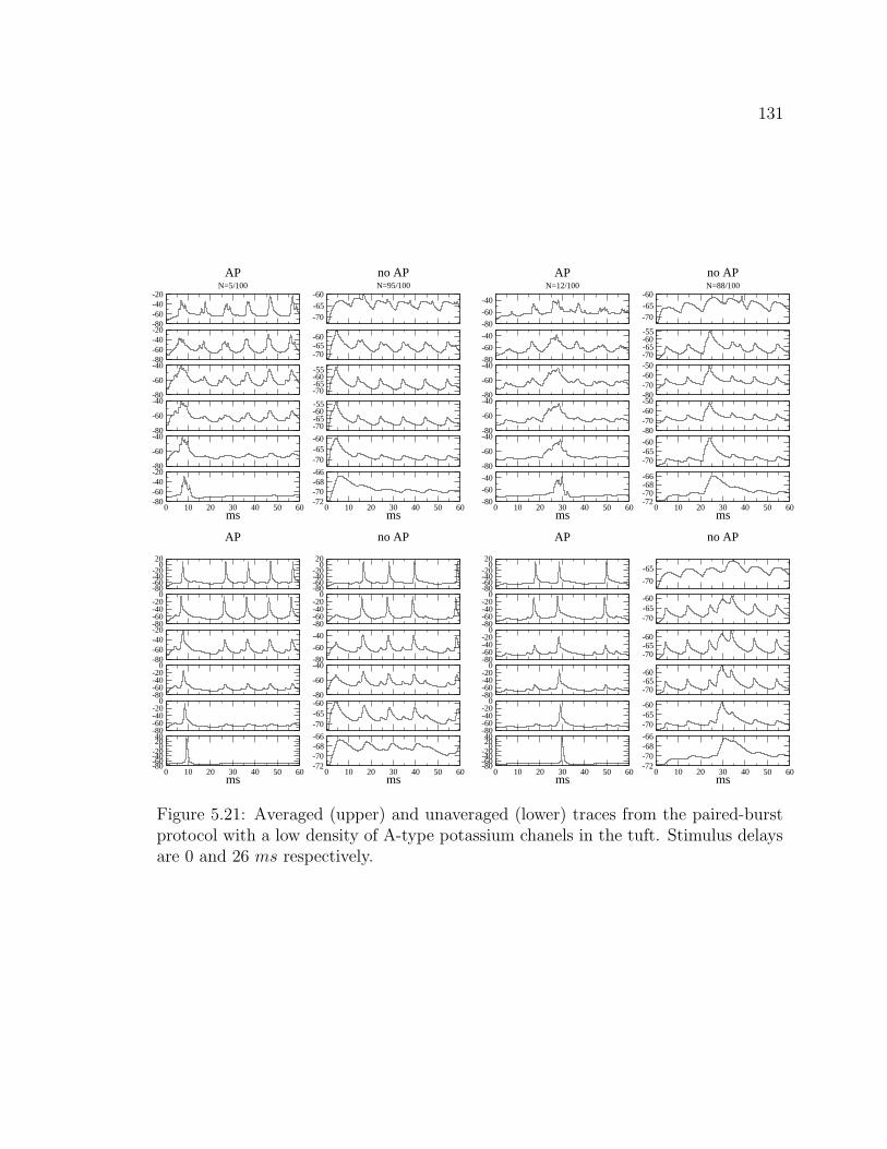
131

-80-60-40-20

APN=5/100

-70-65-60

no APN=95/100

-80-60-40-20

-70-65-60

-80

-60

-40

-70-65-60-55

-80

-60

-40

-70-65-60-55

-80

-60

-40

-70-65-60

0 10 20 30 40 50 60ms

-80-60-40-20

0 10 20 30 40 50 60ms

-72-70-68-66

-80

-60

-40

APN=12/100

-70-65-60

no APN=88/100

-80

-60

-40

-70-65-60-55

-80

-60

-40

-80-70-60-50

-80

-60

-40

-80-70-60-50

-80

-60

-40

-70-65-60

0 10 20 30 40 50 60ms

-80

-60

-40

0 10 20 30 40 50 60ms

-72-70-68-66

-80-60-40-20

020

AP

-80-60-40-20

020

no AP

-80-60-40-20

0

-80-60-40-20

0

-80-60-40-20

-80

-60

-40

-80-60-40-20

0

-80

-60

-40

-80-60-40-20

0

-70-65-60

0 10 20 30 40 50 60ms

-80-60-40-20

02040

0 10 20 30 40 50 60ms

-72-70-68-66

-80-60-40-20

020

AP

-70

-65

no AP

-80-60-40-20

0

-70-65-60

-80-60-40-20

0

-70-65-60

-80-60-40-20

0

-70-65-60

-80-60-40-20

0

-70-65-60

0 10 20 30 40 50 60ms

-80-60-40-20

02040

0 10 20 30 40 50 60ms

-72-70-68-66

Figure 5.21: Averaged (upper) and unaveraged (lower) traces from the paired-burstprotocol with a low density of A-type potassium chanels in the tuft. Stimulus delaysare 0 and 26 ms respectively.

132

generate a Na-spike just at the point of maximal depolarization in the apical dendrite

from SC input.

5.5 Conclusion

The dynamical picture for coincidence detection of TA and SC inputs in CA1 pyrami-

dal cells presented here is experimentally verifiable. Experimental protocols involving

double intracellular recording electrodes have been performed successfully in the past

[82]. Such a double-electrode set-up allows the experimentalist to determine if so-

matic APs are being generated by forward-propagating Na-spikes much as we have

done in figure 5.12.

Stimulating electrodes in TA and SC are needed and stimulus intensities should

be chosen for which either input alone would be mostly subthreshold. Nonetheless,

verification that even subthreshold stimulation via the TA pathway generates Na-

spikes is needed. Verification of localized (no somatic AP) Na-spikes in the proximal

apical dendrites has been made in intracellular recordings [82], which is not possible

in the apical tuft given the very small diameter of the dendrites. Voltage-sensitive

dyes might be a viable alternative.

The ability of CA1 pyramidal cells to act as coincidence detectors for TA and SC

inputs provides a simple mechanistic description of how the two pathways converge

before leaving the hippocampus. Both having originated initially in the entorhinal

cortex, one takes a circuitous route through the dendate gyrus and CA3 region while

the other projects directly to CA1. The output of CA1 pyramidal cells then reflects

the relative timing and intensity of activity coming from these two pathways. This

133

picture is, however, considerably complicated by the presence of inhibitory interneu-

rons and various other intra- and extra-hippocampal projections.

Chapter 6

Excitable Integrate-and-Fire

Neurons in a Small-World Network

6.1 Integrate-and-Fire neurons in networks

One of the major challenges of computational neuroscience is to describe the collective

behavior of many coupled neurons. In the last chapter we saw the lengths to which

it may be necessary to go in order to understand one aspect of the dynamics of just a

single neuron. Even such complex, spatially extended models of neurons are greatly

simplified and most likely fail to capture the full spectrum of dynamical states in

real neurons. To tackle a network of potentially many thousands of neurons seems

daunting indeed.

The hope is that certain simplified dynamical rules may be discerned, which govern

the behavior of single neurons in some parameter regime. Perhaps, for some parameter

values, the state of the neuron lingers near a low-dimensional manifold of an attractor,

134

135

which in its entirety is very large and high-dimensional. In this case, with some

ingenuity and luck, one can formulate a low-dimensional dynamical system to model

the neuronal dynamics. Coupling these systems constitutes a network of neurons.

It is known, for example, that Hodgkin-Huxley type, conductance-based models of

neurons can be broadly classified as either class-I (saddle-node bifurcation on a circle)

or class-II (Hopf bifurcation) excitable depending on the nature of the bifurcation from

the rest state to the firing state. Near this bifurcation, the dynamics can be described

via an asymptotically correct canonical model [85].

Still, the reduction to canonical form assumes that the original, ODE description

of neuronal dynamics is the correct one. In the last chapter we show the importance

of the spatial distribution of inputs in determining the response properties of the

neuron. The fact then remains that the correct choice of model depends crucially on

the specific aspect of neuronal dynamics that the researcher wishes to investigate. If

we mean to study networks we must use reduced models with potentially unjustified

and uncontrolled approximations. There is, as of yet, no alternative.

In this chapter we investigate a network of coupled, excitable integrate-and-fire

neurons (IFN). The IFN is a heuristic model of class I excitability, which is char-

acterized by a vanishing frequency near the bifurcation to repetitive firing. It is a

one-dimensional model:

CdV

dt= −g(V − Vrest) + I,

V (t+) = Vreset whenever V (t−) = Vthreshold, (6.1)

with the reset condition that introduces a discontinuity in the voltage whenever a

136

threshold is exceeded. This discontinuity is meant to model the action potential.

By throwing out information about the amplitude and profile of the action potential,

(6.1) represents a major simplification of neuronal dynamics. Note that in the absence

of external drive, I = 0, the neuron modeled by (6.1) just settles down to its rest

potential. For subthreshold I, the neuron acts as a leaky integrator. Thus (6.1)

describes neuronal dynamics as a linear, subthreshold regime with a sharp threshold

to spiking. This is clearly a cartoon description of a neuron, but nonetheless one that

captures the defining features of neuronal dynamics.

The true advantage of (6.1) becomes apparent when considering a large ensemble

of coupled neurons. We note first that given a fixed, suprathreshold I, the interspike

interval (period of spiking) of the neuron is given by

T = τ ln

(

I/g + (Vrest − Vreset)

I/g − (Vthreshold − Vrest)

)

, τ = C/g, (6.2)

which goes to infinity as I/g → (Vthreshold−Vrest). The result (6.2) is obtained through

simple integration of (6.1). Consider now a network of N coupled neurons, where the

ith neuron evolves according to (6.1) except that the current input I is given by

Ii(t) = I0 + gsyn

N∑

j=1

wij

∫ ∞

0

dτJ(τ)Ej(t− τ), (6.3)

where E and J are the pre-synaptic spikes and post-synaptic responses, respectively.

E might be modelled by a train of delta spikes, one for each action potential fired by

the pre-synaptic cell, and J is typically an α-function or difference of exponentials. In

(6.3), neuron i integrates over all inputs E, which are convolved with its response J ,

137

and if the neurons are connected (wij 6= 0), then this input results in a post-synaptic

current (PSC) with an amplitude proportional to gsyn.

Even for a more complicated current as given by (6.3), we can integrate equation

(6.1) to obtain the firing times of each neuron, which now depend on the firing times

of all the other neurons. The dynamics of such a network of N coupled IFNs is

thus equivalent to N coupled one-dimensional maps. The existence and stability of

phase-locked states can be analyzed straightforwardly for such a system [86].

We can clearly see that all the complication of solving the network equations re-

sides in (6.3), and in particular in the coupling coefficients wij. This is the conceptual

advantage of coupled IFNs: we know the intrinsic dynamics are trivial and that all

the interesting behavior comes about through the particular topology of the network.

The problem is to predict the firing times Ti from the coupling coefficients wij.

The IFN is often proposed as a model to study the collective dynamics of cortical

pyramidal neurons, the most prevalent principal excitatory neuron in the cerebral

cortex. Pyramidal neurons are class-I excitable, and (6.1) is the simplest possible

model of this type. One very robust feature of real cortical neurons is their low,

intrinsic firing rate. This seemingly stochastic background firing is due to the large

number of uncorrelated inputs each cell receives, both from inside and outside the

brain region in which it resides. In the preceeding chapter, for example, we saw that

realistic numbers of synapses for hippocampal pyramidal cells are on the order of

sixty thousand. Cortical neurons generally receive fewer synapses, but still on the

order of tens of thousands. Introducing noise into (6.1) makes the formulation via

coupled maps impractical. In this case, advantageous use has been made of ‘kinetic’

descriptions of the probability distribution for the voltage of the neurons [87, 88, 89]

138

using Fokker-Planck (FP) equations. If the coupling is weak and the inputs mostly

uncorrelated, then the equilibrium states of the FP equations and the instabilities of

these states can be studied with traditional methods of nonlinear analysis.

Fruitful analysis of the coupled-map formulation relies on the network exhibiting

a high degree of symmetry, while the FP formulation can only be meaningfully solved

when the network exhibits disordered dynamics. Unfortunately, it seems that real

cortical networks are somewhere in between [90, 91]. Actual data on the patterns

of synaptic connectivity in the cortex are scarce, but the propagation of waves of

excitation observed in experiment [92] provides evidence for the existence of some

degree of local connectivity. Yet it is also certainly true that long-range excitatory

connections are also present [91, 93]. Finally, neither the local nor the long-range

connections are expected to be completely regular; the network exhibits some degree

of randomness.

While most work in the past has focused on either all-to-all coupling [94, 95, 96,

86], local coupling (such as nearest-neighbor) [97, 86], or random coupling [87, 88, 89],

we shall try to incorporate some aspects of a real cortical network: the coexistence of

local and long-range excitatory connections. This type of network, the small-world

network (SWN) [98], has received much recent interest. The SWN is a regular, local

lattice, complemented with an overlaid network of random connections that may have

any length.

The dynamics of different types of networks of active elements with SWN topology

have been studied. Both relaxational and non-equilibrium dynamics of spin models in

SWNs have been considered [99, 100, 101]. Complex networks of excitable elements

include models for propagation of epidemics [102], where the excited state corresponds

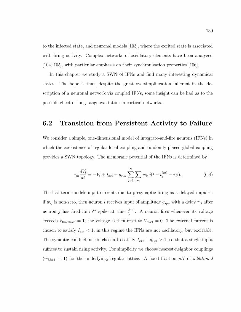
139

to the infected state, and neuronal models [103], where the excited state is associated

with firing activity. Complex networks of oscillatory elements have been analyzed

[104, 105], with particular emphasis on their synchronization properties [106].

In this chapter we study a SWN of IFNs and find many interesting dynamical

states. The hope is that, despite the great oversimplification inherent in the de-

scription of a neuronal network via coupled IFNs, some insight can be had as to the

possible effect of long-range excitation in cortical networks.

6.2 Transition from Persistent Activity to Failure

We consider a simple, one-dimensional model of integrate-and-fire neurons (IFNs) in

which the coexistence of regular local coupling and randomly placed global coupling

provides a SWN topology. The membrane potential of the IFNs is determined by

τmdVi

dt= −Vi + Iext + gsyn

N∑

j=1

∑

m

wijδ(t− t(m)j − τD). (6.4)

The last term models input currents due to presynaptic firing as a delayed impulse:

if wij is non-zero, then neuron i receives input of amplitude gsyn with a delay τD after

neuron j has fired its mth spike at time t(m)j . A neuron fires whenever its voltage

exceeds Vthreshold = 1; the voltage is then reset to Vreset = 0. The external current is

chosen to satisfy Iext < 1; in this regime the IFNs are not oscillatory, but excitable.

The synaptic conductance is chosen to satisfy Iext + gsyn > 1, so that a single input

suffices to sustain firing activity. For simplicity we choose nearest-neighbor couplings

(wi,i±1 = 1) for the underlying, regular lattice. A fixed fraction pN of additional

140

unidirectional couplings wij = 1 is then randomly added to the network.

At p = 0, any excitation sufficient to cause a neuron to fire will generate two

pulses which propagate through the regular lattice in opposite directions with ve-

locity v = 1/τD, and either exit the system or annihilate each other depending on

boundary conditions (see top left panel of figure 6.1 for the case of periodic bound-

ary conditions). No persistent activity results in either case. However, self-sustained

activity may arise for nonzero p. Figure 6.1 shows typical network dynamics for four

values of p (0.0,0.05,0.1,0.15, increasing from top to bottom, left to right). Each panel

contains a raster plot indicating the times at which each neuron fires, and a plot of

the instantaneous firing rate. The addition of long-range connections allows for the

reinjection of activity into the network. This leads naturally to a state of persistent

activity as seen for p = 0.05, 0.1. The firing pattern for p = 0.05 appears highly

regular, and a Fourier spectrum of the instantaneous firing rate (figure 6.2) reveals

a purely periodic pattern. In such a case the activity can truly be called persistent,

since once the system settles into a limit-cycle attractor only external perturbations

could cause the activity to die. For p = 0.15 the activity spreads through the network

but once before dying.

Figure 6.1 merely offers an illustration of some representative dynamics, but it

should be emphasized that for fixed parameter values many different realizations of

the network topology are possible. In fact, for a fixed N and p there are N 2pN possible

network realiztions (the factor of two arises from the choice of a pre- and a post-

synaptic neuron for each global connection). Repeated numerical experimentation

reveals that observation of periodic or higly ordered patterns is typical for low p.

Still, given the random nature of the system, a statistical classification of the network

141

0

200

400

600

800

1000

inde

x

0 100 200 300 400 500t

0

0.0005

0.001

0.0015

0.002

0.0025

0.003

0.0035

0.004

fr

0

200

400

600

800

1000

0 10 20 30 40t

0

0.02

0.04

0.06

0.08

Figure 6.1: Representative raster plots (top of each panel) and instantaneous firingrates (bottom of each panel) for a system of 1000 neurons. Parameter values areIext = 0.85, gsyn = 0.2, τm = 10, τD = 1, p = 0.0, 0.05, 0.1, 0.15 from left to right andtop to bottom. Same parameter values are used in subsequent figures unless otherwisenoted.

142

0 0.1 0.2 0.3 0.4 0.5freq.

0.0001

0.001

0.01

0.1

1/TR

0.02 0.03 0.040.0001

0.001

0.01

Figure 6.2: Fourier spectrum of the instantaneous firing rate for the periodic state(p = 0.05) shown in the upper-right panel in figure 6.1.

dynamics is natural.

In particular, for fixed p, some networks exhibit persistent activity, while in others

the activity rapidly decays. It may be of interest to examine how this transition from

persistent activity to failure occurs in a particular network realization, but we will

restrict our analysis to a probabilistic description of this transition. We will ask:

what is the probability, given fixed parameter values and thus a fixed density of

shortcuts, that a network chosen at random will yield persistent activity? To obtain

these probabilities we calculate long-time averages of the network for many different

realizations. We emphasize that the random, global connectivity is fixed for each

realization and (6.4) thus constitutes a quenched network.

We typically average over 2000 realizations to calculate the probability of persis-

tent activity; the complementary probability of failure to sustain activity is shown

in figure 6.3 as a function of the density p of random connections for four different

system sizes N . In this regime, the probability of failure is an increasing function of

p that crosses over from 0 to 1 with increasing steepness as the size N of the system

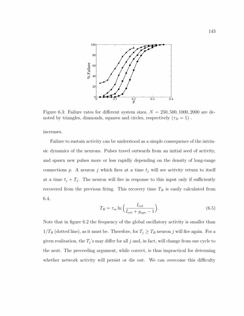
143

0 0.1 0.2 0.3 0.4p

0

20

40

60

80

100

% F

ailu

re

Figure 6.3: Failure rates for different system sizes, N = 250, 500, 1000, 2000 are de-noted by triangles, diamonds, squares and circles, respectively (τD = 1) .

increases.

Failure to sustain activity can be understood as a simple consequence of the intrin-

sic dynamics of the neurons. Pulses travel outwards from an initial seed of activity,

and spawn new pulses more or less rapidly depending on the density of long-range

connections p. A neuron j which fires at a time tj will see activity return to itself

at a time tj + Tj. The neuron will fire in response to this input only if sufficiently

recovered from the previous firing. This recovery time TR is easily calculated from

6.4,

TR = τm ln( Iext

Iext + gsyn − 1

)

. (6.5)

Note that in figure 6.2 the frequency of the global oscillatory activity is smaller than

1/TR (dotted line), as it must be. Therefore, for Tj ≥ TR neuron j will fire again. For a

given realization, the Tj’s may differ for all j and, in fact, will change from one cycle to

the next. The preceeding argument, while correct, is thus impractical for determing

whether network activity will persist or die out. We can overcome this difficulty

144

through a mean-field approximation in which the Tj’s are assumed to be all identical,

and thus depend only on the density of connections p and not the particular topology

of any specific network realization. We make the further assumption that this uniform

value of Tj is equal to the time TA(p) needed for activity to spread throughout the

entire network. This argument assumes that each neuron only receives one input per

cycle, via either a local or a global connection. Equating the recovery time with the

time for activity to spread throughout the network yields the critical density at which

a transition from persistent activity to failure is expected to occur

TA(pcr) = TR. (6.6)

An approximate form for TA(p) is easily derived. We assume that a single neuron

fires at time t = 0. Given a density p of shortcuts we expect a long-range connection

will be reached after 1/p neurons have fired, which occurs after a time τD/2p since

there are two waves. Four wave fronts are now present and so 2/p neurons will fire

in a time τD/2p at which point on average two new wave fronts are generated, and

so on. During the kth cycle, the number of neurons excited is 2k−1/p. After n cycles

all the neurons have been excited, which results in

n−1∑

k=0

2k = pN, (6.7)

which leads to a time

TA(p) =ln (1 + pN)

2p ln 2. (6.8)

Using (6.8) we can solve for pcr(N) in (6.6), and rescale the curves shown in figure

145

0 1 2(p-p

cr(N))/p

cr(N)

0

20

40

60

80

100

% F

ailu

re

Figure 6.4: Failure rates as a function of a rescaled density of shortcuts.

6.3 to obtain figure 6.4. The intersection of all the curves at the predicted critical

value of the density indicates that the transition does indeed occur as hypothesized.

Note, however, the fixed offset of the rescaled curves (the crossing should occur at

zero), due to approximations made in deriving (6.8), as discussed below.

The local dynamics in equation (6.4) are simple: waves travel outward with a

constant velocity 1/τD. Locally, the waves trace out the topology of the network

(although global connections may be traversed in one direction only). The intrinsic

dynamics of the neurons makes the resulting dynamics complex, i.e. the ’tracing-out’

may be hindered if neurons are not sufficiently recovered. Nonetheless, equation (6.8)

is a purely geometric result, since the time it takes for activity to traverse the entire

extent of the network is related trivially to the largest distance in the network.

Mean-field properties of small-world networks have been worked out by Newmann,

Moore and Watts in [107, 108]. In [107] they calculate the fraction of a small-world

network covered by starting at a single point and extending outwards a distance r

in both directions (equivalent to waves having spread for a time rτD in our case) in

146

a continuum limit. In [108] they refine the continuum limit calculation by taking

into account two effects that were omitted from their earlier calculation and from

ours. Firstly, as they trace out the network, a jump via a long-range connection may

reach a part of the network that has already been traced over and should therefore

not be counted. We interpret this as activity spreading via long-range connections,

which may be injected into a neuron which has already fired and is not ready yet.

Such a connection would therefore be ineffectual. Secondly, when two ‘traced-out’

sections meet, they stop and no longer contribute. We interpret this as wavefronts

which meet and annihilate and thus, thereafter, do not contribute. Considering these

two additional mechanisms, they develop a two-component model that describes,

effectively, the fraction of the network covered and the number of fronts. The result,

interpreted within the context of equation (6.4), yields,

√

(

1 +4

pN

)

tanh[

√

(

1 +4

pN

)pTA(p)

2τD

]

= 1. (6.9)

Figure 6.5 shows the failure rates, rescaled by 6.9. The more sophisticated mean-field

model clearly captures the transition correctly.

6.3 Activity for slow waves.

The failure rate may become a non-monotonic function of p for large enough delay

time τD (slow enough waves). Figure 6.6 shows the percentage of realizations in

which the activity has died out within a fixed time (T = 2000) for seven values

of the delay time, increasing from left to right. The first five curves exhibit the

147

-1 -0.5 0 0.5 1(p-p

cr(N))/p

cr(N)

0

20

40

60

80

100

% F

ailu

re

Figure 6.5: Failure rates as a function of the density of shortcuts rescaled accordingto the mean-field model in [108].

transition from persistent activity to failure at low p discussed in the preceeding

section. The failure rate for larger delays is non-monotonic. For τD = 1.6 there is

an initial increase in the percentage of failing realizations as p increases from zero,

in accordance with the analysis from the previous section, but the failure rate does

not saturate at 100%. Rather, it reaches a maximum and decreases at higher values

of p. For yet larger delays, the maximum both shifts to the left and decreases in

magnitude. For sufficiently slow waves, the failure rate (measured at a fixed time)

appears to go to zero for all 0 < p < 1.

Figure 6.7 shows representative patterns of neural activity and firing rates for

slower waves for increasing p (top to bottom, left to right). Most striking is the

contrast between the regular, often periodic patterns seen in the low-p regime, and

the highly disorded patterns seen at values of p near 1. Also clear, especially from

the instantaneous firing rates, is the larger magnitude of the population-oscillation

for high p. In fact, while for a low density of global connections the spread of activity

148

Figure 6.6: Failure rates for a system of 1000 neurons. Curves representing the failurerate after T = 2000 are shown for τD = 0.6, 0.8, 1.0, 1.2, 1.4, 1.6, 1.8, left to right. Thepredicted value of p from equation (6.9) at which the failure transition occurs, is givenby a dotted line for each curve.

appears conspicuously wavelike (see upper-lefthand panel of figure 6.7), at higher

densities the activity spreads extremely rapidly, resulting in a near synchronous firing

of the entire population (see lower-right hand panel of same figure). The Fourier

spectrum for the latter realization is shown in figure 6.8; the spectrum is clearly noisy

although well-defined peaks can be discerned.

The near-synchronous firing of the neurons for high p is not surprising and, in

fact, follows from 6.8; the time needed for activity to spread is a decreasing function

of p for fixed system size. That is, as p increases, the firing of the neurons will be

more and more synchronous. Nonetheless, the re-emergence of persistent activity in

this regime is unexplained by our earlier description. Also unexpected is the high

degree of disorder in the resulting patterns. While the population fires relatively

periodically with a well defined frequency, the individual spikes occur in a seemingly

149

Figure 6.7: Representative raster plots (top of each panel) and instantaneous firingrates (bottom of each panel) for a system of 1000 neurons. Parameter values areIext = 0.85, gsyn = 0.2, τm = 10, τD = 1.6, p = 0.1, 0.2, 0.3, 0.4, 0.5, 0.6, 0.8, 0.9, 1.0,from left to right and top to bottom.

150

0 0.1 0.2freq.

1e-06

0.0001

0.01

1

1/TR

Figure 6.8: Fourier spectrum of the instantaneous firing rate in the lower-right panelof figure 6.7, p = 1.

chaotic manner with respect to this oscillation (see lower panels in figure 6.7). The

resulting patterns appear as noisy homogeneous oscillations in the firing rate. In

addition, modulation of the firing rate on long time-scales is evident.

As a final note on patterns for slow waves, one can see in figure 6.7 that even

for values of p below the persistence-failure transition (top and middle rows), several

qualitative types of patterns can be found. Note, for example, the dynamics exhibited

in the central panel: there is an initial transient of nearly-synchronous population

spikes, as seen to the other side of the transition at high p. However, it seems

that for p not sufficiently large (p = 0.5 in this case) this state is unstable and the

system settles into a highly disordered firing pattern for which the firing rate is almost

constant.

151

The network topology

The drastic change in patterns from low to high p is due to changes in the topology of

the network, as we shall show. The topology of random networks is often characterized

by means of the likelihood of picking a node at random and finding that it has exactly

c connections. This likelihood is given by the degree distribution p(c). In a network

with N nodes and a fixed probability of making a connection p between any two

nodes, the distribution is the binomial distribution

p(c) =

(

N

c

)

pc(1 − p)N−c, (6.10)

which for large N and small p can be approximated by the Poisson distribution

p(c) =(pN)c

c!e−pN . (6.11)

Note that for p = 1 the system is fully connected, i.e. the number of connections is

NN . In our model, a value of p = 1 means that there are N connections. Thus here

p = p/N and 6.11 becomes

p(c) =pc

c!e−p. (6.12)

The degree distribution 6.12 does not apply to our model 6.4, since we have

stipulated that there be exactly pN connections in the network. This choice was

made to facilitate the averaging over many realizations of the network. For the case

where the degree distribution is given by 6.12, not only are there many possible

network topologies for a fixed number of connections, but the number of connections

152

itself is a random variable whose expected value is given by E = pN .

Given that the number of connections is fixed in our model, the relevant degree

distribution must be derived by keeping track of all the nodes. We consider that the

network consists of N nodes of which s0 have no connections, s1 have but a single

connection and, in general, sc have c connections. If the total number of oriented

shortcuts is k, then c may vary between 0 and k. The constraints

s0 + s1 + · · · + sk = N, (6.13)

s1 + 2s2 + · · · + ksk = k, (6.14)

indicate that the probabilities will not be independent as in the Poisson distribution.

The derivation is therefore more involved than that of 6.12. We first note that the

total number of possible shortcut configurations is N k. The probability of a certain

configuration is then just the number of ways to get that configuration divided by

Nk.

The number of ways of getting a certain configuration consists of two parts. First,

we count the number of ways of choosing s0 nodes without any connections. The

remaining nodes can be ordered in (N − so)! ways, but of these many are identical.

For example, the s1 nodes with one connection can be ordered in s1! ways, all of

which are equivalent. Finally, the k connections can be ordered in k! ways, but again

we must be careful not to overcount. For example, a node with 3 connections has 3!

ways to order those connections, and so there are a total of (3!)s3 ways to order the

153

‘triple’ connections in the network. The distribution is then given by

p(s0, s1 . . . , sk) =N !k!

∏ki=0 si!(i!)si

. (6.15)

Note that this is also the appropriate distribution for the case of choosing k times

amongst N objects with replacement. The formula 6.15 is difficult to utilize for

computing expectations. We note that (6.15) satisfies the normalization condition

∑

s0

· · ·∑

sk

p(s0, s1, . . . , sk) = 1, (6.16)

where the upper bounds on the sums are finite and depend on all earlier sums. The

expected number of nodes with 0 ≤ n ≤ k connections is given by

E(sn) =∑

s0

· · ·∑

sk

snp(s0, s1, . . . , sk). (6.17)

Note that the distribution 6.15 is valid both for incoming and outgoing connections.

A numerical calculation of the fraction of neurons with two or more incoming (or

outgoing) connections as a function of the density p is given in figure 6.9. It is evident

that the number of neurons with two incoming connections increases dramatically as

p increases towards 1. In addition, it is clear that the majority of neurons with more

than one incoming connection has exactly two incoming connections for p < 0.4. This

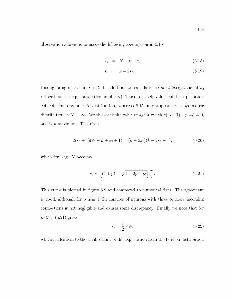
154

observation allows us to make the following assumption in 6.15

s0 = N − k + s2 (6.18)

s1 = k − 2s2 (6.19)

thus ignoring all sn for n > 2. In addition, we calculate the most likely value of s2

rather than the expectation (for simplicity). The most likely value and the expectation

coincide for a symmetric distribution, whereas 6.15 only approaches a symmetric

distribution as N → ∞. We thus seek the value of s2 for which p(s2 + 1)− p(s2) = 0,

and is a maximum. This gives

2(s2 + 1)(N − k + s2 + 1) = (k − 2s2)(k − 2s2 − 1), (6.20)

which for large N becomes

s2 ∼[

(1 + p) −√

1 + 2p− p2]N

2. (6.21)

This curve is plotted in figure 6.9 and compared to numerical data. The agreement

is good, although for p near 1 the number of neurons with three or more incoming

connections is not negligible and causes some discrepancy. Finally we note that for

p 1, (6.21) gives

s2 =1

2p2N, (6.22)

which is identical to the small p limit of the expectation from the Poisson distribution

155

0 0.2 0.4 0.6 0.8 1p

0

0.1

0.2

0.3

0.4

frac

tion

of n

euro

ns

theory for pairspairstriples and higher

Figure 6.9: Fraction of neurons with two or more incoming connections. Shown arepairs (squares) and three or more connections (circles). Solid line is the predictionfrom (6.21).

(6.12). For p near 1, (6.21) yields

s2 =(

1 −√

2

2

)

N − (1 − p)

2N. (6.23)

Comparing this to the value of the expectation for s2 according to the Poisson distri-

bution for p near 1,

E(s2) =1

2eN − (1 − p)

2eN, (6.24)

reveals that assuming a fixed number of connections increases the number of neu-

rons with two incoming connections with respect to the case where the number of

connections is not fixed by a factor of about 1.6 for p = 1.

We thus see that a major topological difference between those networks for which

p ∼ 0.1 and those for which p ∼ 1 is the fraction of neurons with two or more

incoming and outgoing long-range connections. What is the dynamical consequence

of this topological change? One consequence is an increased likelihood that a neuron

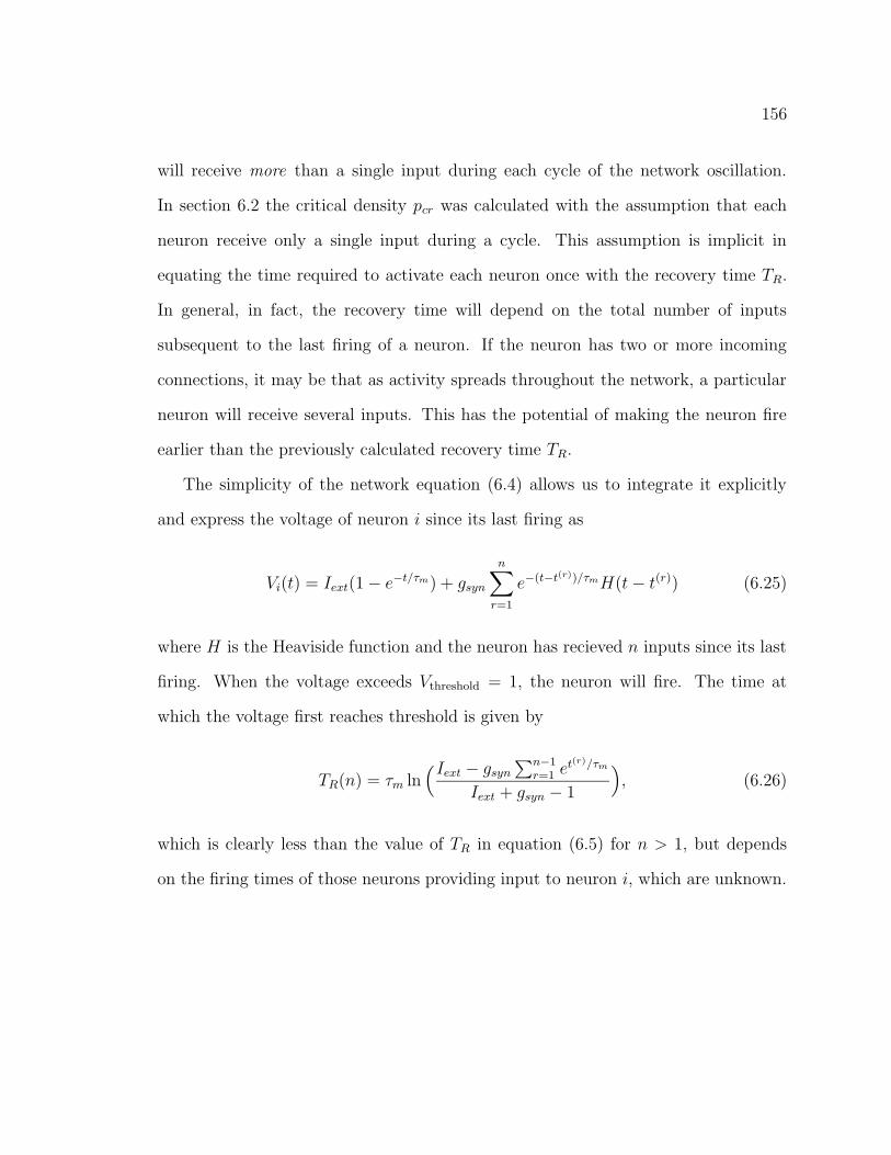
156

will receive more than a single input during each cycle of the network oscillation.

In section 6.2 the critical density pcr was calculated with the assumption that each

neuron receive only a single input during a cycle. This assumption is implicit in

equating the time required to activate each neuron once with the recovery time TR.

In general, in fact, the recovery time will depend on the total number of inputs

subsequent to the last firing of a neuron. If the neuron has two or more incoming

connections, it may be that as activity spreads throughout the network, a particular

neuron will receive several inputs. This has the potential of making the neuron fire

earlier than the previously calculated recovery time TR.

The simplicity of the network equation (6.4) allows us to integrate it explicitly

and express the voltage of neuron i since its last firing as

Vi(t) = Iext(1 − e−t/τm) + gsyn

n∑

r=1

e−(t−t(r))/τmH(t− t(r)) (6.25)

where H is the Heaviside function and the neuron has recieved n inputs since its last

firing. When the voltage exceeds Vthreshold = 1, the neuron will fire. The time at

which the voltage first reaches threshold is given by

TR(n) = τm ln(Iext − gsyn

∑n−1r=1 e

t(r)/τm

Iext + gsyn − 1

)

, (6.26)

which is clearly less than the value of TR in equation (6.5) for n > 1, but depends

on the firing times of those neurons providing input to neuron i, which are unknown.

157

However, the value of TR(n) in equation (6.26) is bounded below by

TR(n) = τm ln( Iext

Iext + ngsyn − 1

)

, (6.27)

which occurs when all n inputs coincide at TR(n) itself. The formula (6.27) reduces

to (6.5) for n = 1.

The time between subsequent spikes of a particular neuron is called the interspike-

interval (ISI). If a neuron only receives a single input per oscillation of the network,

then the ISI is bounded below by TR(1). We can determine the ISI of neurons nu-

merically, in order to indirectly discern between those with a single active incoming

connection and those with several. Figure 6.10 shows the dynamics of a system for

p = 1; all those neurons with ISI less than TR(1) are colored in red. It seems rea-

sonable from this figure to consider the populations of slow and fast spiking neurons

as dynamically distinct. In particular, those neurons with large ISIs (black) undergo

highly synchronized oscillations, the amplitude of which dips to zero. In fact, this os-

cillation should be synchronized and go to zero according to (6.8). However, for large

p there is now a second population of neurons which, by virtue of having received

more inputs over the course of the oscillation, are primed to fire before TR(1). They

carry over the activity in the network until the first population has once again recov-

ered. We further remark that the members of the population of fast-spiking neurons

change from one oscillation to the next. That is, those neurons which are utilized by

the network to bridge the epochs of zero firing rate in the slow-spiking neurons, vary

in a seemingly random manner. In fact, it can be seen in figure 6.10 that there is

a sudden increase in the number of fast-spiking neurons around t = 200, indicating

158

that many more neurons have the potential to fire more quickly than TR(1) than are

typically utilized in a single oscillation.

Figure 6.10: Raster plot (top) and instantaneous firing rate (bottom) for a system of1000 neurons at τD = 1.5 and p = 1.0. Dotted line (bottom) is the total firing rate.Neurons colored red have ISI < TR(1).

Consider also figure 6.11, which contrasts the distribution of ISIs for low (p = 0.1)

and high (p = 1.0) densities of random connections. Note that the ISI appears

bounded below by TR(1) in the former case (solid line), while in the latter there are

fast-spiking neurons with ISI less than TR(1). Figure 6.12, for which p = 0.15 and

τD = 1.0, shows that a small number of neurons actually do have ISIs less than TR(1)

(see inset). Note, in addition, that there is a subset neurons with very long ISIs, as

indicated by the grouping around 130.

159

0 50 100 150ISI

0

0.1

0.2

0.3

0.4

0.5

0.6

0 20 40 60 80ISI

0

0.1

0.2

0.3

0.4

0.5

0.6

0.7

Figure 6.11: Normalized histograms of the ISI for τD = 1.5 and p = 0.1 (left) andp = 1.0 (right). The solid line is TR(1). Data includes ISIs for all 1000 neurons overmany network realizations.

0 50 100 150 200 250 300ISI

0

0.1

0.2

0.3

0.4

0.5

0 50 100 150 200 250 300

ISI0

0.005

0.01

Figure 6.12: Normalized histogram of the ISI for τD = 1.0 and p = 0.15. The solidline is TR(1). Data includes ISIs for all 1000 neurons over many network realizations.

160

Persistence and failure of activity for p ∼ 1

Typical patterns of activity for p ∼ 1 are highly disordered. The absence of a limit-

cycle attractor introduces the possibility that the activity may fail at long times. This

is indeed the case. While in figure 6.6 failure rates are shown for a fixed time T = 2000,

an analogous figure for failure rates determined at a later time, e.g. T = 3000, would

show the portion of the curves for τD = 1.6, 1.8 near p = 1 moving upwards, indicating

more failures. For sufficiently large times T → ∞, it appears that all curves would

tend towards 100% failure for p ∼ 1.

Figure 6.13 shows typical examples of such failure of activity at variable times. The

top panel (τD = 1.4) shows failure occuring after a dozen or so network oscillations.

As the delay is increased, for the exact same network and initial conditions, the

activity persists for longer times (see middle (τD = 1.6) and lower panels (τD = 1.8)).

The trend therefore seems to be towards longer lifetimes for longer delay and this is

true in general.

However, the dependence of the average lifetime on the delay is quite subtle.

Figure 6.14 (left) shows cumulative failure rates for various values of the delay τD as

a function of time. Each curve is determined by finding the times at which failure

occurs in 2000 realizations of a network for fixed parameter values. A histogram of the

frequency of failures binned by time is then made and integrated. Figure 6.14 shows

that the rate of failures indeed decreases as the waves become slower. Nonetheless,

the curves for τD = 1.65 and 1.7 actually cross indicating that the rate of failures

actually decreases as the delay increases from 1.65 to 1.7.

The righthand panel of the same figure indicates that such a scenario is ubiquitous

161

Figure 6.13: Raster plots and instantaneous firing rates for τD = 1.4, 1.6, 1.8 from topto bottom and p = 1. The network topology and all parameters are identical for allthree figures, only the delay has been changed.

162

Figure 6.14: Cumulative distributions f of failure times at p = 1. Dashed lines showfits to stretched exponentials. Right: Failure rates at 5, 10, 20, 40 and 100 multiplesof TR(1) = 28.3, black to brown. Symbols are averages of 2000 realizations.

as a function of the delay. The percentage of persistent realizations are shown as a

function of the delay at 5 different fixed times (see caption for times), increasing from

the top to the bottom curve. The high degree of structure shows that the failure times

depend sensitively on the delay. The non-monotonic nature of the curves furthermore

points to the fact that there are preferred values of the delay (locally speaking) for

which activity persists longer. Such values might be considered ‘resonant’.

The cummulative failure rates in figure 6.14 are well fit by a stretched exponential

function of the form

f = f∞ − ce−αtβ , (6.28)

where the value f∞ gives the percentage of realizations for which activity will have

failed at infinite time. While the fits are good, the coefficients obtained from fitting

the data in figure 6.14 to this form are not reliable. Table 6.1 shows some sample

fit values; 1 the data has been fitted starting from Ts = 0, 1000 and 5000. The

1All fits were done with the intrinsic non-linear curve-fitting function in xmgrace.

163

0 20000 40000 60000 80000t

0

20

40

60

80

100f

Ts = 0Ts = 1000Ts = 5000

0 20000 40000 60000 80000t

-2

-1

0

1

2

f-f fi

t

Ts=0Ts=1000Ts=5000

Figure 6.15: Left: Stretched exponential fits to cumulative failure rates. Here τD =1.6. Fits are to data with 0 < t < Ts. Right: Difference between cummulative failurerate and stretched exponential fit.

Ts f∞ c α β0 100 80.6 0.015 0.558

1000 100 88.2 0.017 0.5505000 100 678 0.330 0.290

Table 6.1: Coefficients of stretched exponential fit.

coefficients vary non-monotonically and do not converge. In fitting many such curves

for various starting and ending times, at no point were the coefficients found to

converge. Nonetheless, figure 6.15 (left) shows that the three curves given by these

coefficients are nearly indistinguishable from each other and fit the data well. The

difference between the cummulative failure rates and the fits (figure 6.15, right) show

that deviations are not random and seem to have an oscillatory time dependence.

As a note on the use of a stretched exponential fit, if we assume that each realiza-

tion has a probability of failure pf and that these probabilities are distributed across

realizations according to ρ(pf ), then the percentage of failures over many realizations

164

is given by

< f(t) >= 100(1 −∫ ∞

0

dpfρ(pf )e−pf t). (6.29)

Equation 6.29 is known to have a stretched exponential solution of the form< f(t) >=

100(1 − e−αtβ) for β = 1/2 when

ρ(pf ) =1

2p3/2f

√

γ

πe− γ

4pf , (6.30)

with γ = α1/β [109].

The trend towards longer life-times for larger delay τD can be explained simply. In

order to bridge the quiescent periods between near-synchronous firing of the popula-

tion of slow-spiking neurons (ISI ≥ TR(1)), the network makes use of those neurons

which, having received additional excitation during the oscillation, are primed to fire

earlier than TR(1). Such neurons must be arranged in a topological chain so that they

can be activated one after another. If such a chain has length l, the time bridged via

this chain is l ·τD. Thus, given a fixed topology, more and more chains can be utlilized

as τD increases. Put another way, the probability that the quiescent period can be

bridged must depend on the distribution of available chains and the time bridged

by each chain. Because the time bridged by each chain goes up as τD increases, the

likelihood that the quiescent period will be successfully bridged also increases.

6.4 Bistability and Noise

One of the salient features of the emergent dynamics of the model (6.4) in the presence

of random, long-range connections is persistent self-sustained activity in the low p

165

Figure 6.16: Raster plot (top) and instantaneous firing rate (bottom) for a system of1000 neurons and 100 interneurons (p = 0.10) with k = 5. Noise causes the neurons tofire stochastically but is insufficient to generate traveling pulses. About 10 adjacentneurons are stimulated synchronously at t = 250; 20% of the neurons are activatedat t = 750 to turn the active state off.

regime. In this regime the network is in fact bistable between ‘off’ and ‘on’ states,

and can be switched between them with a sufficiently large stimulus, as illustrated

in figure 6.16. The synchronous stimulation of a sufficiently large number of neurons

while the network is in the ‘on’ state will increase the level of activity and effectively

push the network above the failure transition (cf. figure 6.3), causing a transition

into the ‘off’ state.

Network bistability has been hypothesized to be the neural correlate underlying

the type of short-term memory known as ‘working’ memory in the prefrontal cortex

of monkeys and humans. Much more realistic and physiologically plausible models of

cortical layers have been studied within the context of working memory (e.g. [110]).

The central feature of all such models is the ability of the network to sustain elevated

166

activity through recurrent excitatory connections. Not much attention has been given

to heterogeneities in network topology or to long-range excitatory connections. The

work presented here suggests a closer look at the possible role of these factors in

generating and maintaining the active state in more realistic models.

Central to the computational usefulness of bistability in the level of activity of

a network is its robustness to perturbation. For neural networks in particular, such

external perturbations are often in the form of a low level of noisy background activ-

ity due to the integration of many uncorrelated inputs. Such inputs result in a low,

seemingly stochastic firing rate in real cortical neurons (a few Hz). We note that the

current model is not robust to noise levels sufficient to elicit spikes, since this would

trivially initiate the on-state of the network. Such ‘epileptic’ behavior is to be ex-

pected from (6.4) since we have neglected the stabilizing influence of inhibition. This

system could be viewed as a coarse-grained model, in which each neuron represents a

small emsemble of neurons (cortical column). The firing of a neuron then represents

the synchronized output from this small ensemble, while the non-firing state of the

neuron may include low-level, non-synchronous firing within the ensemble.

A more realistic model that would allow for comparison with realistic firing rates,

would include both inhibition and a topologically more complex local coupling. As

an example of how modifiying the local coupling alone can already make the network

more robust to noise, we extend the local excitatory coupling to include up to 2k

neighbors (wi,i±j = 1 for j = 1 . . . k) and model long-range connections via a popu-

lation of intermediate excitatory neurons which both receive input from and project

to multiple adjacent neurons. Under these conditions, spontaneous activity is highly

unlikely to initiate traveling pulses; a sufficiently large stimulus, synchronous across

167

several neurons, is needed to turn the state of elevated activity on and off (cf. figure

6.16).

Even in the presence of noise, the probabilistic transition from persistent activity

to failure is expected to occur, given that the noise intensity is not too large. For

larger amplitude noise, qualitatively new behavior is seen. Consider figure 6.17, which

shows the firing rate of a typical network for fast waves (τD = 1.0) and eight different

values of the noise amplitude increasing from top to bottom, left to right (note that

k = 1 again). Gaussian noise with amplitude a is added to the model. Note that

Gaussian noise may drive the neuron towards threshold or lower its voltage, in the

latter case reflecting some inhibitory input.

The upper two panels of figure 6.17 show the case of a low density of global

connections p = 0.1. We will refer to noise levels [1] through [8]. We see a periodic

pattern in the absence of noise (top left [1]). The addition of noise can actually

cause the network to switch between a number of distinct periodic patterns [2] (see

figure 6.18). Larger amplitude noise causes the pattern to break up and become

disordered [3] and sufficiently strong noise can even turn the activity off [4]. Once the

noise is sufficiently strong to force the firing rate to zero one can properly speak of

population bursts. The length of the burst decreases for increasing noise amplitude

[5], [6] although the bursting itself is intermittent and does not appear to have a

well-defined period. Even stronger noise causes the mean inter-burst interval (IBI) to

shrink to zero [7], [8].

The lower two panels of figure 6.17 show the case of a high density of global

connections (p = 1.0), for which activity always fails in the absence of noise [1].

The presence of noise causes synchronized population spikes [2]. Isolated spikes occur

168

Figure 6.17: The effect of noise on the instantaneous firing rate in a system of 1000neurons. Parameters are τD = 1.0 and p = 0.1, 1.0 for the top and bottom fig-ures respectively. Noise amplitude is a = 0.0, 0.1, 0.2, 0.3 (upper-left) 0.4, 0.5, 0.6, 0.7(upper-right) 0.0, 0.4, 0.45, 0.5 (lower-left) and 0.55, 0.6, 0.65, 0.7 (lower-right).

169

Figure 6.18: Noise can cause networks with low p to switch between various, appar-ently periodic attractors. The figure shows four distinct patterns which arose duringthe course of a single simulation for p = 0.1, a = 0.01 and τD = 1.0. Over a dozendistinct patterns arose during the course of this simulation which was ended at a timeT = 20000.

precisely because the network activity dies out after a single oscillation in this regime.

Increasing the noise reduces the ISI [3], [4] and even causes some intermittent bursting

if sufficiently strong [5]. Increasing the noise even further reduces the interval between

population spikes to zero [7], [8].

Note that the persistence-failure transition discussed in section 6.2 can now be

reinterpreted for various levels of noise. Section 6.2 deals with case [1], a = 0. For

case [2] the transition is between a regular firing state in which the system explores

various periodic attractors to a state of highly synchronous population spikes. For

case [4] there is a transition with increasing p between population bursting with very

long IBI (note that this run was not sufficiently long to include more than a single

burst), and population spiking with relatively shorter ISI.

Figure 6.19 shows the effect of noise for slow waves; τD = 1.6. Four values of p

are shown (0.1, 0.4, 0.7, 1.0) from top to bottom. For p = 0.1 the patterns are much

170

as before, ranging from a switching between attractors [2] through bursting [5].

For p = 1.0, where activity in the absence of noise is long-lived [1], the addition

of noise can cause activity to fail early [2]. The noisy dynamics are essentially in-

distinguishable from the case where noise is absent, at least as far as the firing rate

is concerned. The only discernible effect is the reduction in amplitude of the mod-

ulation of the firing rate as the noise is increased [3]-[8]. The cases p = 0.4, 0.7 are

intermediate in nature to p = 0.1 and p = 1.0.

6.5 Conclusion

We have investigated the types of network activity in the model defined by equation

(6.4) as a function of the parameters p, τD and a which measure the density of global

connections, the inverse of the speed of the waves and the noise intensity, respectively.

Figure 6.20 shows a schematic representation of the network behavior as a function

of these three variables, and summarizes the findings we have presented thus far.

One additional interesting aspect of the dynamics in the low p regime is the

existence of a unique ‘pathway’ of activity. This ‘pathway’ is defined for a fixed

network and intial condition, as the subset of neurons that, if disconnected from

the rest of the network, would continue to propagate the activity normally. Consider

figure 6.21, in which the ‘pathway’ is highlighted in red. Ignoring the initial transient,

once the system has settled into a limit cycle only those neurons in red are needed

to propagate the activity. The ‘pathway’ is determined by looking at the state of the

system at long times and retracing the activity backwards, highlighting only those

neurons which caused other neurons to fire later on.

171

We note, finally, that many of the details of the network dynamics are not fully

understood. In particular, the distribution of topological chains and the use of these

chains dynamically, as briefly remarked upon at the end of section 6.3, is a difficult

question and, as yet, an unanswered one.

172

Figure 6.19: The effect of noise on the instantaneous firing rate in a system of 1000neurons. Parameters are τD = 1.6 and p = 0.1, 0.4, 0.7, 1.0 going from top to bottom.The noise amplitude for each value of p ranges between 0.0 and 0.07 from top tobottom, left to right.

173

0 0.2 0.4 0.6 0.8 1p

0

0.5

1

1.5

2

τ D

periodic

persistent

no activity

long-lived

disordered

0 0.2 0.4 0.6 0.8 1p

0

0.5

1

1.5

2

τ D

switching

periodic

population spikes

long-lived

disordered

0 0.2 0.4 0.6 0.8 1p

0

0.5

1

1.5

2

τ D

bursting

population spikes

long-lived

disordered

Figure 6.20: Schematic phase diagram of the network behavior for no noise, lowamplitude, and high amplitude noise, respectively (left to right).

Figure 6.21: An activity ‘pathway’ (see text) for p = 0.05 and τD = 1.0.

Appendix A

Derivation of amplitude equations

Here we outline the derivation of the amplitude equation (2.47) which describes the

slow-time evolution of modulations of plane waves in (2.23, 2.24). We consider finite-

wavenumber modulations pcr of waves with wavenumber qcr as given by (2.43) and

(2.42). We first expand the phase and C-field as,

φ

C

=

qcrX

0

+ εΦ0 + ε2Φ1 + . . . , (A.1)

where ε =√

a−a0

a2and a0 is the value of the control parameter at onset of the fastest-

growing mode. We rewrite (2.23, 2.24) symbolically as,

L

φ

C

+ N (φ,C) = 0, (A.2)

174

175

and expand the linear and nonlinear operators in ε,

L = L0 + εL1 + ε2L2 + . . . , (A.3)

N = ε2N1 + ε3N2 + . . . , (A.4)

DE = D + ε2D2, (A.5)

with

L0 =

D∂2X − ∂T

qcr

R2 ∂X

−2hqcr∂2X δ∂2

X − ∂T − α2 + (s+ h)∂X

, (A.6)

L1 = 0, (A.7)

L2 =

D2∂2X − ∂τ R2∂X

0 −∂τ

, (A.8)

N1 =

(

K1C∂2Xφ+K2∂Xφ∂

2Xφ+K3C∂XC +K4∂Xφ∂XC, −2h∂Xφ∂

2Xφ

)T

,(A.9)

N2 =

K5∂2Xφ(∂Xφ)2 +K6C

2∂2Xφ+K7C∂Xφ∂

2Xφ+K8(∂Xφ)2∂XC+

K9C∂XC∂Xφ+K10C2∂XC, 0

T

.

(A.10)

176

where the coefficients are given by,

R =√

a0 − q2cr, R2 = −a2qcr

R4, (A.11)

D =R2 − 2q2

cr

R2, D2 =

a2

R2(1 −D), (A.12)

K1 =(1 −D)

R2, K2 =

2qcrR2

(D − 3), (A.13)

K3 = −qcrR4, K4 =

1

R2(1 +

2q2cr

R2), (A.14)

K5 =1

R2(D − 3 − 8a0q

2cr

R4), K6 = −2qcr

R6, (A.15)

K7 =4qcrR6

(q2cr + a0), K8 =

qcrR4

(3 +4q2

cr

R2), (A.16)

K9 = − 1

R4(1 +

4q2cr

R2), K10 =

qcrR6. (A.17)

The slow time is given by τ = ε2T . At order ε we recover the homogeneous,

linearized system,

L0Φ0 = 0. (A.18)

The zero-mode Φ0 we take, as in 3.1, to be of the form,

Φ0 =

Φ0

C0

A0(τ)e

i(pcrX+ωcrT ) + c.c. (A.19)

The eigenvector (Φ0, C0)T is determined by solving (A.18),

Φ0

C0

=

iqcrpcr

R2

Dp2cr + iωcr

(A.20)

177

The left-null eigenvector is found by solving the adjoint problem,

Φ†0

=

2hqcrp2cr

Dp2cr − iωcr

ei(pcrX+ωcrT ). (A.21)

At O(ε2) we have

L0Φ1 +N1(Φ0) = 0. (A.22)

The nonlinear term N1 contributes both spatio-temporally homogeneous modes

and modes of twice the critical modulation. We thus take Φ1 to be of the form,

Φ1 =

Φ12

C12

A2

0e2i(pcrX+ωcrT ) + c.c+

TΦ10

C10

|A0|2. (A.23)

With this ansatz, (A.22) reduces to two linear, algebraic systems. The system

corresponding to the forced second harmonic is

−4Dp2cr − 2iωcr 2ipcr

qcr

R2

8hqcrp2cr −4δp2

cr − α + 2i(s+ h) − 2iωcr

Φ12

C12

+

K1Φ0C0p2cr + iK2Φ

20p

3cr − iK3C

20pcr +K4Φ0C0p

2cr

−2ihΦ20p

3cr

= 0, (A.24)

178

and that for the homogeneous forcing

−1 0

0 −α

Φ10

C10

+

−K1p2cr(Φ

∗0C0 + Φ0C

∗0 ) +K4p

2cr(Φ

∗0C0 + Φ0C

∗0 )

0

= 0.(A.25)

Note that the homogeneous forcing causes a response in the phase which grows linearly

with time, i.e. it changes the frequency of the wave (cf. (A.23)).

At O(ε3) we have

L0Φ2 + L2Φ0 + N1(Φ0,Φ1) + N1(Φ1,Φ0) + N2(Φ0,Φ0,Φ0) = 0. (A.26)

At this order the critical Fourier mode appears through the nonlinear forcing terms

and the action of the linear operator L2 on the eigenvalue of the linearized operator

of the original system. In order for a solution to exist, these contributions must lie

orthogonal to the left nullspace of the operator L0. We thus obtain the solvability

condition,

〈Φ†0

∗, L2Φ0 + N1(Φ0,Φ1) + N1(Φ1,Φ0) + N2(Φ0)〉 = 0, (A.27)

where the inner product is defined as an integral over one period of the critical Fourier

mode and the scalar product of the scalar vectors in Φ, C-space. The solution of (A.27)

results in a differential equation (2.47) for the complex amplitude A0, the expression

for which is extremely long and involved.

Here we follow the same procedure as in the previous derivation in outlining the

179

derivation of the Landau equation for the amplitude-driven instability. The calcu-

lation is carried out at bandcenter, i.e. q = 0. We perturb the basic, plane-wave

state in equations (2.50, 2.51) by expanding the real amplitude R and real field C in

ε =√

a−a0

a2where a0 is defined as in Appendix A,

R

C

=

√a0

0

+ εΨ0 + ε2Ψ1 + . . . . (A.28)

We rewrite (2.50, 2.51) symbolically as,

L

R

C

+ N (R,C) = 0. (A.29)

We now expand the linear and nonlinear operators in ε,

L = L0 + εL1 + ε2L2 + . . . , (A.30)

N = ε2N1 + ε3N2 + . . . , (A.31)

180

with

L0 =

∂2x − ∂t − 2a0

√a0

2h√a0∂x δ∂2

x − ∂t − α + s∂x

, (A.32)

L1 = 0, (A.33)

L2 =

−2a2 − ∂τa2

2√

a0

h a2√a0∂x −∂τ

, (A.34)

N1 =

(

RC − 3√a0R

2, 2hR∂xR

)T

, (A.35)

N2 =

(

−R3, 0

)T

.

(A.36)

At order ε we recover the homogeneous, linearized system,

L0Ψ0 = 0. (A.37)

The zero-mode Ψ0 we take, as in 4.1, to be of the form,

Ψ0 =

R0

C0

A0(τ)e

i(pcrX+ωcrt) + c.c. (A.38)

The eigenvector (R0, C0)T is determined by solving (A.37),

R0

C0

=

√a0

p2cr + iωcr + 2a0

. (A.39)

181

The left-null eigenvector is found by solving the adjoint problem,

Ψ†0

=

−2h√a0ipcr

p2cr + 2a0 − iωcr

ei(pcrX+ωcrT ). (A.40)

At O(ε2) we have

L0Ψ1 +N1(Ψ0) = 0. (A.41)

The nonlinear term N1 contributes both spatio-temporally homogeneous modes

and modes of twice the critical modulation. We thus take Ψ1 to be of the form

Ψ1 =

R12

C12

A2

0e2i(pcrX+ωcrT ) + c.c+

R10

C10

|A0|2. (A.42)

With this ansatz, (A.41) reduces to two linear, algebraic systems. The system

corresponding to the forced second harmonic is

−4p2cr − 2iωcr − 2a0

√a0

4h√a0ipcr −4δp2

cr − 2iωcr − α + 2ispcr

R12

C12

+

R0C0 − 3√a0R

20

2ihpcrR20

= 0, (A.43)

182

and that for the homogeneous forcing

−2a0

√a0

0 −α

R10

C10

+

R0C∗0 +R∗

0C0 − 6√a0|R0|2

0

= 0. (A.44)

Solving these systems yields the following expression for the scalar quantities,

R12 =m12

d12

, (A.45)

C12 =n12

d12

, (A.46)

m12 = −1

2

√

a0(4a0δp2cr + 4δp4

cr + a0α + p2crα + 2ωcrspcr − 2ω2

cr + i[4δp2crωcr

+αωcr − 2a0spcr − 2sp3cr + 2a0ωcr + 2ωcrp

2cr + 2a0hpcr]), (A.47)

n12 = −4a0hpcr

(

−ωcr + i[a0 +3

2p2

cr]

)

, (A.48)

d12 = −8δp4cr − 2(α + 2a0δ)p

2cr − a0α + 2ωcr(ωcr − spcr)

i[4sp3cr − 4ωcr(1 + δ)p2

cr + 2a0pcr(s+ h) − ωcr(2a0 + α)], (A.49)

R10 = −√

a0 +1√a0

(p2cr + 2a0), (A.50)

C10 = 0. (A.51)

At cubic order projection onto the left null eigenvector yields the amplitude equa-

tion for A0,

∂τA0 = l(pcr)(p2cr + iωcr)A0 + l(pcr)

√

a0

[C12

√

a0 − 3a03/2 + 2R12(p

2cr − a0) + 2R10(p

2cr − a0 + iωcr)]|A0|2A0,(A.52)

l(pcr) = 2ihpcr(p2

cr + 2a0)2 − ω2

cr − 2i[ωcr(p2cr + 2a0) + ha0pcr]

[(p2cr + 2a0)2 − ω2

cr]2 + 4[ωcr(p2

cr + 2a0) + ha0pcr]2. (A.53)

Appendix B

Derivation of Peierls-Nabarro

potential

Here we outline the derivation of the Peierls-Nabarro potential for a kink in the FK

model in the limit of weak coupling (k → 0). We begin by solving for the stable and

unstable configurations given by

sinxi = k(xi+1 − 2xi + xi−1) + f. (B.1)

Outside the region of distortion caused by the defect, the solution to B.1 is

xn = 2πn+ ψ (B.2)

where ψ = sin−1 f .

183

184

The defect region of the stable configuration is given by

x1 = 2πn+ ψ

x2 = 2π(n+ 1) + ψ − x2

x3 = 2π(n+ 1) + ψ + x3

x4 = 2π(n+ 2) + ψ. (B.3)

We solve B.1 with xi = x2 which upon expanding in the small parameters x2, x3

yields

x2 =2πk

√

1 − f 2+ O(k2) (B.4)

where we note that cosψ =√

1 − f 2. Solution of B.1 with xi = x3 reveals x3 = x2.

The defect region of the unstable configuration is given by

x1 = 2πn+ ψ + x1,

x2 = 2π(n+ 1) + π − ψ + x2,

x3 = 2π(n+ 2) + ψ + x3,

x4 = 2π(n+ 3) + ψ. (B.5)

Solving B.1 for xi where i = 1, 2, 3 respectively results in the linear system

√

1 − f 2 + 2k −k 0

−k −√

1 − f 2 + 2k −k

0 −k√

1 − f 2 + 2k

x1

x2

x3

=

−k(π + 2ψ)

4kψ

k(π − 2ψ)

(B.6)

185

the soution of which is

x1 =−k(π + 2ψ)√

1 − f 2+ O(k2), (B.7)

x2 =−4kψ√

1 − f 2+ O(k2), (B.8)

x3 =k(π − 2ψ)√

1 − f 2+ O(k2). (B.9)

The energies of both the stable and unstable configurations are given by

E =N∑

i=0

(

k

2(xi+1 − xi− 2π)2 + 1 − cos xi

)

(B.10)

which yields equations 4.31 and 4.32.

Note however, that these expressions break down as f → 1. In this limit we scale

k = O(ε)

f = 1 − εf

xi = O(ε1/2)

which leads to, for the stable configuration

x2 = −√

2f1/2(

1 −√

1 +2πk

f

)

, (B.11)

x3 =

√

2f1/2(

1 −√

1 − 2πk

f

)

, (B.12)

186

and for the unstable configuration

x1 =

√

2f(

1 −√

1 +k(π + 2ψ)

f

)

, (B.13)

x2 = −√

2f(

1 −√

1 − 4kψ

f

)

, (B.14)

x3 =

√

2f(

1 −√

1 − k(π − 2ψ)

f

)

. (B.15)

Using B.10 we arrive at equations 4.36 and 4.37.

Appendix C

Probabilities for defect generation

The variable-density Frenkel-Kontorova (vdFK) equation is given by 4.2 coupled to

a rule for determining the number of particles in the chain which varies in time and

space N(x, t). As a simple rule we will consider the case that there is a probability

that a particle is added p+dt and a probablity that one is taken away p−dt in a time

dt. In this case, the probability that a particles have been added in a time t is given

by

p(a, t) =

(

n

a

)

p+a(1 − p+)n−a (C.1)

where n = tdt

and p+ = p+dt. This is simply a binomial distribution, which for long

times (and small dt) can be approximated as a poisson distribution

p(a, t) ∼ (p+t)a

a!e−p+t. (C.2)

The probability density function pdf for s is found by C.1 with a→ s and p+ → p−.

We are concerned not with the number of particles added or taken away, but with

187

188

the number of defects present d = |a−s|. We first note that the probability of having

added a particles and taken away s particles is just

p(a, s) = p(a)p(s) = p(s)p(a) = p(s, a). (C.3)

The probability of d defects is given by

p(|a− s| = d) = p(s = a+ d) + p(a = s+ d) = p(a, a+ d) + p(s+ d, s)

= 2n−d∑

u=0

p(u+ d, u) d 6= 0 (C.4)

which makes use of C.3. For d = 0 we have clearly overcounted by a factor of two, so

p(d = 0) =n∑

u=0

p(u, u). (C.5)

We choose the probabilities

p+ = p+ α[(s− a)]+ (C.6)

p− = p+ α[(a− s)]+ (C.7)

where [(·)]+ is the positive rectifying function. The term proportional to α reflects

the fact that the system prefers a state with no defects a = s.

189

Figure C.1: Left: The probability of the defect-free state as a function of time (notethat n is proportional to time, i.e. n = t

dt) for p = 0.15. Lines are from C.8 (black)

and C.10 (red). Right: The probability of a single (top) and eight defects (bottom).Lines are C.8 (black), C.13, (red) and C.15 (blue).

For α = 0 the sums C.5 and C.4 can be expressed in closed form 1 , yielding

p(d) =

(1 − p)2n(

1 − ( p1−p

)2)nP 0

n

[

1+( p1−p

)2

1−( p1−p

)2

]

d = 0

2(

nd

)

(1 − p)2n−2dΓ(1 + d)(

1 − ( p1−p

)2)nP−d

n

[

1+( p1−p

)2

1−( p1−p

)2

]

d > 0(C.8)

where P−dn is the Legendre function of degree n and order −d. Figure C.2 shows

typical histograms for the number of added particles and the number of defects.

An alternative form for p(d) can be derived in the limit of large n and small p. It is

analogous to the derivation of the poisson distribution from the binomial distribution.

Consider first the probability for d = 0

p(u, u) =n∑

u=0

[

(

n

u

)

pu(1 − p)n−u]2

. (C.9)

1The properties of Legendre, Bessel, and Hypergeometric functions can be found in [111]

190

Substituting p = λn, we take the limit n→ ∞ keeping λ fixed, yielding

p(d = 0) =∞∑

u=0

(λ)2u

(u!)2e−2λ

= Io(2pt)e−2pt (C.10)

where Io is the 0th order modified Bessel function. The probability for nonzero d can

similarly be written

p(d) =n−d∑

u=0

(

n

u+ d

)(

n

u

)

p2u+k(1 − p)2n−2u−k (C.11)

where we rewrite

p(d) =n−k∑

u=0

[

(

n

u

)

pu(1 − p)n−u]2

k∏

r=1

((n− u− k + r)

(u+ r)

)( p

1 − p

)k

. (C.12)

We now take the step of letting n → ∞ while allowing for the possibility that the

difference n− k may not be large, thus retaining it in the initial sum

p(d) = 2λke−2λ

n−k∑

u=0

λ2u

(u!)2

Γ(n− u+ 1)Γ(u+ 1)

Γ(u+ k + 1)Γ(n− u− k + 1)

1

nk

(

1 − λ

n

)−k

= 2

(

λ(

1 − λn

)

)k

e−2λ Γ(n+ 1)

nkΓ(1 + k)Γ(n− k + 1)

·F ([−n+ k], [−n, 1 + k], λ2) (C.13)

where F is the generalized Hypergeometric function. Finally, making use of the

191

0 5 10 150

0.05

0.1

0.15

0.2

0.25added particlesnumber of defects

0 2 4 6 8 10 120

0.05

0.1

0.15

0.2

0.25α=0.0001α=0.001

Figure C.2: Left: Numerically generated histograms for the number of added particlesand number of defects respectively. Symbols are predictions from C.1 and C.8 forn = 50 and p = 0.1. Right: Histograms for nonzero α. Symbols are from C.16.

relationship

limn→∞

nkP−dn (x) = Id(na cosh x) (C.14)

we can take the limit n→ ∞ in C.8 yielding

p(d) =

I0(2pt)e−2pt d = 0

2Γ(1+k)k!

Ik(2pt)e−2pt d > 0

(C.15)

where Ik is the kth order modified Bessel function. Figure C.1 shows that all the above

forms for the probability give equivalent results. Equations C.15 have a particularly

convenient form for integration in time. The case α = 0 is unfortunately not of

interest for comparison to MD simulations.

192

0 0.0005 0.001 0.0015 0.002 0.0025p

0

0.5

1

1.5

<d>

Figure C.3: Long time mean of the number of defects as a function of p for α = 0.001.

For α 6= 0 we have, making use of C.3,

p(d, α) =

p(d, 0) d = 0

2∑n−k

u=0

(

nu+d

)(

nu

)

pu+k(1 − p)n−u+kpu(1 − p)n−u d > 0(C.16)

where p = p+ α · d.

The quantitity of interest for the determination of the slip velocity in 4.67 is the

expected number of defects at long time since if limt→∞E(d(t)) = do where do is a

constant, then one can choose a T sufficiently large such that

limT→∞

1

T

∫ T

0

dtE(d(t)) ∼ limT→∞

1

T

[

∫ T

0

dtE(d(t)) +

∫ T

T

dtdo

]

= do. (C.17)

See figure C.3.

References

[1] F. Charru, P. Barthelet, Secondary instabilities of interfacial waves due to cou-

pling with a long wave mode in a two-layer Couette flow, Physica D 125 (1999)

311.

[2] B. Malomed, Patterns produced by a short-wave instability in the presence of

a zero mode, Phys. Rev. A 45 (1992) 1009.

[3] H. Riecke, Self-trapping of traveling-wave pulses in binary mixture convection,

Phys. Rev. Lett. 68 (1992) 301.

[4] H. Riecke, Ginzburg-Landau equation coupled to a concentration field in binary-

mixture convection, Physica D 61 (1992) 253–259.

[5] M. Ipsen, P. Soerensen, Finite wavelength instabilities in a slow mode coupled

complex Ginzburg-Landau equation, Phys. Rev. Lett. 84 (2000) 2389–2392.

[6] P. Matthews, S. Cox, Pattern formation with a conservation law, Nonlinearity

13 (2000) 1293–1320.

193

194

[7] P. Bartelet, F. Charru, Benjamin-Feir and Eckhaus instabilities with galilean

invariance: the case of interfacial waves in viscous shear flows, Eur. J. Mech.,

B/Fluids 17 (1998) 1–18.

[8] M. Renardy, Y. Renardy, Derivation of amplitude equations and analysis of

sideband instabilities in two-layer flows, Phys. Fluids 5 (1993) 2738.

[9] A. Bernoff, Finite amplitude convection between stress-free boundaries;

Ginzburg-Landau equations and modulation theory, Euro. J. Appl. Math. 5

(1994) 267.

[10] E. Siggia, A. Zippelius, Pattern selection in Rayleigh-Benard convection near

threshold, Phys. Rev. Lett. 47 (1981) 835.

[11] F.H.Busse, E.W.Bolton, Instabilities of convection rolls with stress-free bound-

aries near threshold, J.Fluid Mech. 146 (1984) 115–125.

[12] P. Kolodner, Drifting pulses of traveling-wave convection, Phys. Rev. Lett. 66

(1991) 1165.

[13] W. Barten, M. Lucke, M. Kamps, Localized traveling-wave convection in binary

fluid mixtures, Phys. Rev. Lett. 66 (1991) 2621.

[14] H. Riecke, G. Granzow, Localization of waves without bistability: Worms in

nematic electroconvection, Phys. Rev. Lett. 81 (1998) 333.

[15] M. Dennin, G. Ahlers, D. Cannell, Chaotic localized states near the onset of

electroconvection, Phys. Rev. Lett. 77 (1996) 2475.

195

[16] P. C. Matthews, S. M. Cox, One dimensional pattern formation with Galilean

invariance near a stationary bifurcation, Phys. Rev. E 62(2) (2000) R1473.

[17] H. Riecke, Solitary waves under the influence of a long-wave mode, Physica D

92 (1996) 69–94.

[18] C. Martel, J. Vega, Dynamics of a hyperbolic system that applies at the onset

of the oscillatory instability, Nonlinearity 11 (1998) 105.

[19] G. Kuppers, D. Lortz, Transition from laminar convection to thermal turbulence

in a rotating fluid layer, J. Fluid Mech. 35 (1969) 609.

[20] R. Clever, F. Busse, Nonlinear properties of convection rolls in a horizontal

layer rotating about a vertical axis, J. Fluid Mech. 94 (1979) 609.

[21] F. Busse, K. Heikes, Convection in a rotating layer: a simple case of turbulence,

Science 208 (1980) 173.

[22] Y. Hu, R. Ecke, G. Ahlers, Convection under rotation for Prandtl numbers near

one: I. linear stability wavenumber selection and pattern dynamics, Phys. Rev.

E 55 (1997) 6928.

[23] Y. Hu, W. Pesch, G. Ahlers, R. Ecke, Convection under rotation for Prandtl

numbers near one:II Kuppers-Lortz instability, Phys. Rev. E 58 (1998) 5821.

[24] K. L. Thompson, K. M. Bajaj, G. Ahlers, Traveling concentric-roll patterns in

Rayleigh-Benard convection with modulated rotation, Phys. Rev. E 65 (2002)

046218.

196

[25] Y. Ponty, T. Passot, P. Sulem, A new instability for finite Prandtl number

rotating convection with free-slip boundary conditions, Phys. Fluids 9 (1997)

67.

[26] M. Neufeld, R. Friedrich, H. Haken, Order-parameter equation and model equa-

tion for high Prandtl number Rayleigh-Benard convection in a rotating large

aspect ratio system, Z. Phys. B 92 (1993) 243.

[27] A. Mancho, H. Riecke, F. Sain, Instabilities and spatio-temporal chaos of long-

wave hexagon patterns with rotation, Chaos 12 (2002) 706.

[28] J. Millan-Rodriguez, C. Perez-Garcia, M. Bestehorn, M. Fantz, R. Friedrich,

Pattern formation in convection of rotating fluids with broken vertical symme-

try, Phys. Rev. A 46 (1992) 4729.

[29] M. Fantz, R. Friedrich, M. Bestehorn, H. Haken, Pattern-formation in rotating

Benard convection., Physica D 61 (1992) 147.

[30] F. Sain, H. Riecke, Instabilities and spatio-temporal chaos of hexagonal patterns

with broken chiral symmetry, Physica D 144(1-2) (2001) 124.

[31] M. Cross, D. Meiron, Y. Tu, Chaotic domains: a numerical investigation, Chaos

4 (1994) 607.

[32] S. L. Pollicott, P. C. Matthews, S. M. Cox, Instability of convection in a fluid

layer rotating about an oblique axis, Phys. Rev. E 67 (2003) 016301.

[33] A. Roxin, H. Riecke, Rotating convection in an anisotropic system, Phys. Rev.

E 65 (2002) 046219.

197

[34] R. Worthing, The stability of infinite Prandtl number rotating conduction,

Phys. Lett. A 237 (1998) 381.

[35] R. E. Kelly, The onset and development of Rayleigh-Benard convection in shear

flows: A review, in Physiochemical Hydrodynamics, edited by D. B. Spalding

1987, p.65 .

[36] G. A. Y. Hu, R. Ecke, Behavior of focus patterns in low Prandtl number con-

vection, Phys. Rev. Lett. 72 (1994) 2191.

[37] R. Ecke, Y. Hu, R. Mainieri, G. Ahlers, Excitation of spirals and chiral sym-

metry breaking in Rayleigh-Benard convection, Science 269 (1995) 1704.

[38] G. A. Y. Hu, R. Ecke, Convection near threshold for Prandtl numbers near one,

Phys. Rev. E 48 (1993) 4399.

[39] W. Pesch, (private communication).

[40] V. Moroz, (private communication).

[41] Y. Pomeau, P. Manneville, Wavelength selection in axisymmetric cellular struc-

tures, J. Phys. (Paris) 42 (1981) 1067.

[42] M. C. Cross, P. G. Daniels, P. C. Hohenberg, E. D. Siggia, Phase-winding

solutions in a finite container above the convective threshold, J. Fluid Mech.

127 (1983) 155.

[43] P. Hohenberg, L. Kramer, H. Riecke, Effects of boundaries on one-dimensional

reaction-diffusion equations near threshold, Physica 15D (1985) 402–420.

198

[44] L. Kramer, E. Ben-Jacob, H. Brand, M. Cross, Wavelength selection in systems

far from equilibrium, Phys. Rev. Lett. 49 (1982) 1891.

[45] H.-G. Paap, H. Riecke, Drifting vortices in ramped Taylor vortex flow: quanti-

tative results from phase equation, Phys. Fluids A 3 (1991) 1519.

[46] R. Pit, H. Hervet, L. Leger, Direct experimental evidence of slip in hexadecane:

Solid interfaces, Phys. Rev. Lett. 85(5) (2000) 980.

[47] Y. Zhu, S. Granick, Rate-dependent slip of a Newtonian liquid at smooth sur-

faces, Phys. Rev. Lett. 87(9).

[48] V. S. J. Craig, C. Neto, D. R. M. Williams, Shear-dependent boundary slip in

an aqueous Newtonian liquid, Phys. Rev. Lett. 87(5) (2001) 054504.

[49] E. Bonaccurso, M. Kappl, H. J. Butt, Hydrodynamic force measurements:

Boundary slip of water on hydrophilic surfaces and electrokinetic effects, Phys.

Rev. Lett. 88(7) (2002) 076103.

[50] E. Bonaccurso, H.-J. Butt, V. S. J. Craig, Surface roughness and hydrodynamic

boundary slip of a Newtonian fluid on a completely wetting system, Phys. Rev.

Lett. 90(14) (2003) 144501.

[51] P. A. Thomson, M. O. Robbins, Shear flow near solids: Epitaxial order and

flow boundary conditions, Phys. Rev. A 41(12) (1990) 6830.

[52] P. A. Thomson, S. M. Troian, A general boundary condition for liquid flow at

solid surfaces, Nature 389 (1997) 360.

199

[53] J.-L. Barrat, L. Bocquet, Large slip effect at a nonwetting fluid-solid interface,

Phys. Rev. Lett. 82(23) (1999) 4671.

[54] M. Cieplak, J. Koplik, J. R. Banavar, Boundary conditions at a fluid-solid

interface, Phys. Rev. Lett. 86(5) (2001) 803.

[55] O. M. Braun, Y. S. Kivshar, Nonlinear dynamics of the Frenkel-Kontorova

model, Physics Reports 306 (1998) 109.

[56] L. M. Floria, J. J. Mazo, Dissipative dynamics of the Frenkel-Kontorova model,

Advances in Physics 45(6) (1996) 505.

[57] F. G. Bass, Y. S. Kivshar, V. V. Konotop, Y. A. Sinitsyn, Dynamics of solitons

under random perturbations, Physics Reports 157(2) (1988) 63.

[58] Y. S. Kivshar, B. A. Malomed, Dynamics of solitons in nearly integrable sys-

tems, Rev. Mod. Phys. 61(4) (1989) 763.

[59] D. Menzel, Water on a metal surface, Science 295 (2002) 8.

[60] S. Aubry, P. Y. L. Daeron, The twist map, the extended Frenkel-Kontorova

model and the devil’s staircase, Physica D 8 (1983) 381.

[61] S. N. Coppersmith, D. S. Fisher, Pinning transition of the discrete sine-Gordon

equation, Phys. Rev. B 28(5) (1983) 2466.

[62] T. Strunz, F.-J. Elmer, Driven Frenkel-Kontorova model. I Uniform sliding

states and dynamics domains of different particle densities, Phys. Rev. E 58(2)

(1998) 1601.

200

[63] T. Strunz, F.-J. Elmer, Driven Frenkel-Kontorova model. II. Chaotic sliding

and nonequilibrium melting and freezing, Phys. Rev. E 58(2) (1998) 1612.

[64] M. Paliy, O. Braun, T. Dauxios, B. Hu, Dynamical phase diagram of the dc-

driven underdamped Frenkel-Kontorova chain, Phys. Rev. E 56(4) (1997) 4025.

[65] O. M. Braun, A. R. Bishop, J. Roder, Hysteresis in the underdamped driven

Frenkel-Kontorova model, Phys. Rev. Lett. 79(19) (1997) 3692.

[66] O. M. Braun, Y. S. Kivshar, Kinks in a system of adatomic chains, J. Phys.:

Condens. Matter 2 (1990) 5961.

[67] B. Ermentrout, Type I membranes, phase resetting curves, and synchrony, Neu-

ral Computation 8 (1996) 979.

[68] C. Willis, M. El-Batanouny, P. Stancioff, Sine-Gordon kinks on a discrete lat-

tice. i. Hamiltonian formalism, Phys. Rev. B 33(3) (1986) 1904.

[69] S. N. Coppersmith, D. S. Fisher, Threshold behavior of a driven incommensu-

rate harmonic chain, Phys. Rev. A 38(12) (1988) 6338.

[70] B. Li, D. Y. Kwok, Discrete Boltzmann equation for microfluidics, Phys. Rev.

Lett. 90(12) (2003) 124502.

[71] V. P. Sokhan, D. Nicholson, N. Quirke, Fluid flow in nanopores: An examination

of hydrodynamic boundary conditions, J. of Chem. Phys. 115(8) (2001) 3878.

[72] S. Lichter, A. Roxin, S. Mandre, Slip at a liquid-solid interface, preprint .

[73] M. J. Z. et al. (Ed.), Fundamental Neuroscience, Academic Press, 1999.

201

[74] D. G. Amaral, M. P. Witter, The Rat Nervous System, 2nd Edition, Academic

Press, Inc., 1995, Ch. Hippocampal Formation, p. 443.

[75] T. F. Freund, G. Buzsaki, Interneurons of the hippocampus, Hippocampus 6

(1996) 347.

[76] R. Bartesaghi, T. Gessi, Activation of perforant path neurons to field CA1 by

hippocampal projections, Hippocampus 13 (2003) 193.

[77] P. Vetter, A. Roth, M. Hausser, Propagation of action potentials in dendrites

depends on dendritic morphology, J. Neurophysiol 85 (2001) 926.

[78] N. L. Golding, W. L. Kath, N. Spruston, Dichotomy of action-potential back-

propagation in CA1 pyramidal neuron dendrites, J. Neurophysiol 86 (2001)

2998.

[79] M. Migliore, D. A. Hoffman, J. C. Magee, D. Johnston, Role of an A-type K+

conductance in the back-propagation of action potentials in the dendrites of

hippocampal pyramidal neurons, J. Comp. Neuroscience 7 (1999) 5.

[80] M. Megias, Z. Emri, T. F. Freund, A. I. Gulyas, Total number and distribution

of inhibitory and excitatory synapses on hippocampal CA1 pyramidal cells,

Neuroscience 102 (2001) 527.

[81] G. Stuart, N. Spruston, B. Sakmann, M. Hausser, Action potential initiation

and backpropagation in neurons of the mammalian CNS, TINS 20 (1997) 125.

202

[82] N. L. Golding, N. Spruston, Dendritic sodium spikes are variable triggers of

axonal action potentials in hippocampal CA1 pyramidal neurons, Neuron 21

(1998) 1189.

[83] M. Remondes, E. M. Schumann, Direct cortical input modulates plasticity and

spiking in CA1 pyramidal neurons, Nature 416 (2002) 736.

[84] J. Trimmer, (private communication) .

[85] E. M. Izhikevich, Class I neural excitability: conventional synapses, weakly

connected networks, and mathematical foundations of pulse-coupled models,

IEEE 10 (1999) 499.

[86] P. C. Bressloff, S. Coombes, A dynamical theory of spike train transitions in

networks of integrate-and-fire oscillators, SIAM J. Appl. Math. 60 (2000) 820.

[87] N. Brunel, V. Hakim, Fast global oscillations of integrate-and-fire neurons with

low firing rates, Neural Computation 11 (1999) 1621.

[88] N. Brunel, Dynamics of networks of randomly connected excitatory and in-

hibitory spiking neurons, J. Physiol. (Paris) 94 (2000) 445.

[89] N. Brunel, Dynamics of sparsely connected networks of excitatory and in-

hibitory spiking neurons, J. Comp. Neuroscience 8 (2000) 183.

[90] V. B. Mountcastle, The columnar organization of the neocortex, Brain 120

(1997) 701.

203

[91] G. Gonzalez-Burgos, G. Barrionuevo, D. A. Lewis, Horizontal synaptic con-

nections in monkey prefrontal cortex: An in vitro electrophysiological study,

Cerebral Cortex 10 (2000) 82.

[92] J.-Y. Wu, L. Guan, Y. Tsau, Propagating activation during oscillations and

evoked responses in neocortical slices, J. Neurosci. 19 (1999) 5005.

[93] R. Demir, L. B. Haberly, M. B. Jackson, Epileptiform discharges with in-vivo-

like features in slices of rat piriform cortex with longitudinal association fibers,

J. Neurophys. 86 (2001) 2445.

[94] C. van Vreeswijk, L. F. Abbott, Self-sustained firing in populations of integrate-

and-fire neurons, SIAM J. Appl. Math. 53 (1993) 253.

[95] D. Hansel, G. Mato, C. Meunier, Synchrony in excitatory neural networks,

Neural Computation 7 (1995) 307.

[96] P. C. Bressloff, S. Coombes, Desynchronization, mode locking and bursting in

strongly coupled integrate-and-fire oscillators, Phys. Rev. Lett. 81 (1998) 2168.

[97] P. H. Chu, J. G. Milton, J. D. Cowan, Connectivity and the dynamics of

integrate-and-fire neural networks, Int. J. Bif. Chaos 4 (1994) 237.

[98] D. J. Watts, S. H. Strogatz, Collective dynamics of ‘small world’ networks,

Nature 393 (1998) 440.

[99] A. D. Sanchez, J. Lopez, M. A. Rodriguez, Nonequilibrium phase transitions in

directed small-world networks, Phys. Rev. Lett. 88 (2002) 048701.

204

[100] A. Pekalski, Ising model on a small-world network, Phys. Rev. E 64 (2001)

057104.

[101] B. J. Kim, H. Hong, P. Holme, G. S. Jeon, P. Minnhagen, M. Y. Choi, XY

model in small-world networks, Phys. Rev. E 64 (2001) 056135.

[102] M. Kuperman, G. Abramson, Small world effect in an epidemiological model,

Phys. Rev. Lett. 86 (2001) 2909.

[103] L. F. Lago-Fernandez, R. Huerta, F. Corbacho, J. A. Siguenza, Fast response

and temporal coherent oscillations in small-world networks, Phys. Rev. Lett. 84

(2000) 2758.

[104] M. Barahona, L. M. Pecora, Synchronization in small-world systems, Phys. Rev.

Lett. 89 (2002) 054101.

[105] H. Hong, M. Y. Choi, B. J. Kim, Synchronization on small-world networks,

Phys. Rev. E 65 (2002) 026139.

[106] X. F. Wang, G. Chen, Synchronization in small-world dynamical netoworks,

Int. J. Bif. Chaos 12 (2002) 187.

[107] M. E. J. Newman, D. J. Watts, Scaling and percolation in the small-world

network model, Phys. Rev. E 60 (1999) 7332.

[108] M. E. J. Newmann, C. Moore, D. J. Watts, Mean-field solution of the small-

world network model, Phys. Rev. Lett. 84 (2000) 3201.

205

[109] J. D. G. Eran Rabani, B. J. Berne, Direct observation of stretched-exponential

relaxation in low-temperature Lennard-Jones systems using the cage correlation

function, Phys. Rev. Lett. 82 (1999) 3649.

[110] A. Compte, N. Brunel, P. S. Goldman-Rakic, X.-J. Wang, Synaptic mechanisms

and network dynamics underlying spatial working memory in a cortical network

model, Cereb. Cortex 10 (2000) 910.

[111] M. Abramowitz, I. Stegun (Eds.), Handbook of Mathematical Functions, Dover,

1972.