North Dakota Implementation of Mechanistic-Empirical Pavement Design Guide (MEPDG)

MPC 14-274 | Pan Lu, Andrew Bratlien, and Denver Tolliver

Colorado State University North Dakota State University South Dakota State University

University of Colorado Denver University of Denver University of Utah

Utah State UniversityUniversity of Wyoming

A University Transportation Center sponsored by the U.S. Department of Transportation serving theMountain-Plains Region. Consortium members:

Understanding Mechanistic-Empirical Pavement Design Guide (MEPDG) for

North Dakota Implementation

Dr. Pan Lu

Associate Research Fellow

Andrew Bratlien

Transportation Research Engineer

Dr. Denver Tolliver

Director

Upper Great Plains Transportation Institute

North Dakota State University, Fargo

December 2014

Acknowledgements

This research was made possible with funding from the Mountain-Plains Consortium (MPC). The authors

express their deep gratitude to MPC.

Disclaimer

The authors alone are responsible for the preparation and the accuracy of the information presented in this

report. The document is disseminated under the sponsorship of the Mountain-Plains Consortium in the

interest of information exchange. The U.S. Government assumes no liability for the contents or use

thereof.

North Dakota State University does not discriminate on the basis of age, color, disability, gender expression/identity, genetic information, marital status, national origin, public assistance status, sex, sexual orientation, status as a U.S. veteran, race or religion. Direct inquiries to the Vice President for Equity, Diversity and Global Outreach, 205 Old Main, (701) 231-7708.

ABSTRACT

North Dakota currently designs roads based on the AASHTO Design Guide procedure, which is based on

the empirical findings of the AASHTO Road Test of the late 1950s. However, limitations of the current

empirical approach have prompted AASHTO to move toward the new mechanistically based pavement

design procedure described in the Mechanistic Empirical Pavement Design Guide (MEPDG), which was

released to the public for review in 2004 under NCHRP Project 1-37A. MEPDG combines mechanistic

and empirical methodology and provides more realistic characterization of in-service pavements. Its

mechanistic approach is both more thorough and more computationally complex than the existing

AASHTO design method, and as a result the method can require an extensive number of detailed

material, foundational, traffic, and environmental inputs. This and other factors can present a challenge to

agencies wishing to implement the new method.

Because AASHTO has adopted the MEPDG and highway agencies across the nation are moving towards

its implementation, it is critical that North Dakota becomes familiar with the MEPDG documentation and

software and identify input data requirements for design. This report summarizes the findings of MEPDG

implementation in North Dakota, identifies input data needs and research steps of the MEPDG

implementation in the state and also prepares North Dakota for successful implementation of the MEPDG

statewide.

TABLE OF CONTENTS

1. INTRODUCTION ................................................................................................................................ 1

1.1 Background ...................................................................................................................................... 1 1.2 Research Objectives ......................................................................................................................... 2 1.3 Report Organization ......................................................................................................................... 2

2. PAVEMENT DESIGN PROCEDURES ............................................................................................ 3

2.1 The AASHTO 1993 Design Guide .................................................................................................. 3 2.1.1 AASHO Road Test and Various Versions of the Design Guide ......................................... 4 2.1.2 AASHTO 1993 Design Guide Inputs ................................................................................. 5 2.1.3 Limitations of AASHTO Design Guide ............................................................................. 7

2.2 The Mechanistic-Empirical Pavement Design Guide (MEPDG) .................................................... 7 2.2.1 Design Approach ................................................................................................................ 8 2.2.2 Inputs .................................................................................................................................. 8 2.2.3 Pavement Modeling .......................................................................................................... 11

3. LOCAL CALIBRATION OF MEPDG ............................................................................................ 15

3.1 Steps for Local Calibration ............................................................................................................ 15 3.1.1 Step 1: Select Hierarchical Input Level for Each Input Parameter ................................... 16 3.1.2 Step 2: Develop Local Experimental Plan and Sampling Template ................................. 16 3.1.3 Step 3: Estimate Sample Size for Each Distress Prediction Model .................................. 16 3.1.4 Step 4: Select Roadway Segments .................................................................................... 16 3.1.5 Step 5: Extract and Evaluate Roadway Segment Data ..................................................... 17 3.1.6 Step 6: Conduct Field and Forensic Investigations ........................................................... 18 3.1.7 Step 7: Assess Local Bias from Global Calibration Values .............................................. 18 3.1.8 Step 8: Eliminate Local Bias of Distress and IRI Prediction Models ............................... 19 3.1.9 Step 9: Assess the Standard Error of the Estimate ............................................................ 20 3.1.10 Step 10: Reduce the Standard Error of the Estimate ......................................................... 21 3.1.11 Step 11: Interpretation of Results, Deciding on Adequacy of Calibration Parameters ..... 21

3.2 Challenges of Using Pavement Management System (PMS) Data for MEPDG ........................... 24 3.2.1 Project Data....................................................................................................................... 24 3.2.2 Traffic Data ....................................................................................................................... 24 3.2.3 Pavement Structure ........................................................................................................... 24 3.2.4 Materials Data ................................................................................................................... 25

4. SENSITIVITY ANALYSIS ............................................................................................................... 26

4.1 Early Calibration Research ............................................................................................................ 26 4.2 NCHRP Report 1-47 ...................................................................................................................... 27 4.3 Buch et al. 2013 ............................................................................................................................. 28

5. AASHTOWARE PAVEMENT ME DESIGN SOFTWARE ......................................................... 30

5.1 Open Project .................................................................................................................................. 31 5.2 General Information ....................................................................................................................... 33 5.3 Performance Criteria ...................................................................................................................... 34 5.4 Pavement Structure and Material ................................................................................................... 34

5.4.1 Property Grid .................................................................................................................... 36 5.5 Traffic ............................................................................................................................................ 40 5.6 Climate ........................................................................................................................................... 43 5.7 Analysis ......................................................................................................................................... 45

5.8 Reporting ....................................................................................................................................... 46 5.9 Optimization .................................................................................................................................. 46

6. RECOMMENDATIONS FOR FUTURE RESEARCH ................................................................. 47

REFERENCES .......................................................................................................................................... 48

LIST OF FIGURES

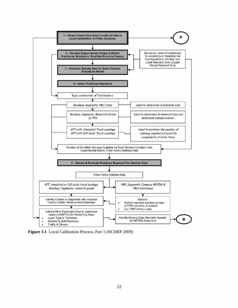
Figure 3.1 Local Calibration Process, Part 1 (NCHRP 2009) ................................................................... 22

Figure 3.2 Local Calibration Process, Part 2 (NCHRP 2009) ................................................................... 23

LIST OF TABLES

Table 2.1 Traffic Input Parameters .............................................................................................................. 9

Table 2.2 Material Input Parameters ......................................................................................................... 10

Table 2.3 Environmental Input Parameters ............................................................................................... 10

Table 3.1 Calibration Parameters by Distress Type ................................................................................... 20

Table 4.1 NCHRP 1-47 Global Sensitivity Analysis (GSA) Results ........................................................ 28

Table 4.2 Buch et al. GSA Results ............................................................................................................ 29

1

1. INTRODUCTION

1.1 Background

The 1993 version of the American Association of State Highway and Transportation Officials (AASHTO)

Guide for the Design of Pavement Structures is currently the primary document used to design new and

rehabilitated highway pavements in the United States. According to a 2007 FHWA survey (FHWA 2007),

63% of state DOT’s use the 1993 design procedure. AASHTO 1993 design equations were based on the

empirical findings of the AASHO Road Test, conducted from 1958 to 1960 in Ottawa, Illinois. The Road

Test was conducted in a single geographical location on a limited number of flexible and rigid pavement

sections and subjected to a limited number and type of traffic loads. In that sense, the empirical

relationships derived from the Road Test are truly representative only of the conditions present at the

Road Test in Illinois. Moreover, the models developed and modified from the Road Test only relate key

pavement properties and traffic to performance and do not consider the climatic effects.

In order to overcome the limitations of the existing design method, the AASHTO Joint Task Force on

Pavements, in conjunction with the National Cooperative Highway Research Program (NCHRP) in

NCHRP Report 1-37A, developed the Mechanistic-Empirical Pavement Design Guide (MEPDG). The

new MEPDG procedure involves three major steps:

1. Use the known mechanistic properties of materials to compute the internal material responses in

deflections, stresses, and strains in a trial design when subjected to predicted future traffic and

climatic factors.

2. Convert predicted material response to accumulated pavement damages in terms of cracking,

rutting, and smoothness. Repeat steps 1 and 2 until pavement performance passes the design

criteria.

3. Continue testing trial designs; select the best one based on life cycle cost analysis and other

considerations.

The Mechanistic-Empirical Pavement Design Guide (MEPDG) is being widely implemented and used by

many highway agencies across the nation. As of 2007 (FHWA 2007), 80% of states have an MEPDG

implementation plan and many of them consider the MEPDG as the goal for future pavement design and

analysis. Moreover, AASHTO is expected to adopt the MEPDG in the future. However, a number of

challenges in successful MEPDG implementation have been identified. Understanding these challenges is

important for agencies considering implementing the Guide.

First, MEPDG models require an extensive amount of input, including detailed traffic spectra, pavement

material properties, and environmental conditions. The procedures, training, and personnel required to

collect much of these data is neither easy or inexpensive; moreover, preparation of the collected data to

meet the MEPDG input requirement can also be challenging.

Further, the new MEPDG models were nationally calibrated and validated using Long-Term Pavement

Performance (LTPP) data from the Federal Highway Administration (FHWA). However, nationally

calibrated models can have limited accuracy in local applications because of significant differences

between national and local traffic and environmental and material properties. As such, it is critical that

MEPDG models be calibrated and validated for local conditions before they are implemented on an

agency-wide level.

2

1.2 Research Objectives

The goal of this research is to prepare North Dakota to successfully implement MEPDG. Objectives

include:

To compare the principle, major inputs, and distress models of the two design procedures (1993

Design and MEPDG)

To identify the input data needs for local calibration of MEPDG flexible pavement distress

models in North Dakota

To perform a review of sensitivity analysis literature, identifying key input parameters that are

most significant to MEPDG pavement performance predictions

To document procedures of the new AASHTOWare Pavement ME-Design software

1.3 Report Organization

This section is the introduction of the organization of the report. Section 2 summarizes the flexible

pavement design procedures of AASHTO 1993 and MEPDG. Section 3 introduces the need for local

calibration, including identification and summarization of the requirements for collecting input data.

Section 4 addresses sensitivity analysis and identifies MEPDG input variables which have the most

significant impact on pavement performance predictions. Section 5 introduces and documents the

procedures and steps necessary to design and analyze flexible pavements in the current version of

AASHTOWare ME-Design software, build 1.3.29. Finally, Section 6 summarizes the conclusions and

recommendations from this study.

3

2. PAVEMENT DESIGN PROCEDURES

North Dakota Department of Transportation (NDDOT) currently designs its highway pavements in

accordance with the AASHTO Guide for Design of Pavement Structures. The AASHTO guide has long

been widely accepted as the standard in pavement design, with versions released in 1961, 1972, 1986, and

most recently in 1993. The guide is fundamentally based upon empirical models built from field

performance data collected at the AASHO Road Test in Ottawa, Illinois, from 1958 to 1960. The design

method not only calculates required thicknesses of pavement layers but also evaluates pavement

performance in terms of surface distresses due to traffic loading over pavement design life.

Empirical pavement design methods are typically based on prediction equations or curves derived from

field or laboratory data. The relationships built from field data are typically verified against performance

expectations or engineering judgment. In general, the overall serviceability of a pavement section is often

modeled using a relationship between traffic, typically measured by a single index, such as Equivalent

Single Axle Load (ESAL), and a composite performance index which represents combined distresses.

A mechanistic design approach, in contrast, is based on theories of mechanics of structural behavior and

uses, for example, layered elastic analysis to calculate internal elastic strains induced by traffic loads and

environmental conditions.

Mechanistic-empirical design is a hybrid procedure. It involves calculating elastic strains in pavement in

response to traffic load and environmental conditions based on mechanics theory. These structural

responses are then linked to stress predictions from empirical models. National Cooperative Highway

Research Program (NCHRP) Project 1-37A (NCHRP, 2004) developed the most recent M-E based model

to predict distresses by traffic load and environmental conditions. The NCHRP 1-37A project also

incorporated national calibration models and detailed vehicle load spectra. The NCHRP also released a

companion computational software, DARWin-ME, which has since been rebranded AASHTOWare

Pavement ME Design. The latest software build as of this writing is 1.3.29.

The majority of state transportation agencies currently utilize AASHTO 1993 empirical design, although

many have implemented or have begun to implement the new MEPDG. A 2007 survey by FHWA found

that 63% of state DOTs currently use the AASHTO 1993 design guide and 80% of state DOTs have plans

for MEPDG implementation. The current AASHTO 1993 guide and the MEPDG design procedure for

flexible pavement will be described in the following sections.

2.1 The AASHTO 1993 Design Guide

The AASHTO 1993 design approach produces a required pavement structure from an empirical design

equation with traffic, material, and climatic inputs. The output, layer thicknesses, are deterministically

calculated using the design equation.

The first version of the AASHTO Design Guide was released in 1961 as the “AASHO Interim Guide for

the Design of Rigid and Flexible Pavements.” All versions of the AASHTO design guide were based on

the results of the AASHO Road Test. The AASHO Road Test and evolution of the AASHTO Guide will

be introduced in this section, followed by the 1993 design equations and input requirements.

4

2.1.1 AASHO Road Test and Various Versions of the Design Guide

The AASHO Road Test studied structural performance of pavements with known thickness under moving

loads of known magnitude and frequencies (HRB 1961). It was designed to investigate, through a series

of experiments, the relationship between repeated traffic loading and highway pavement deterioration.

The road test was carried out from October 1958 to November 1960 in Ottawa, Illinois. The seven-mile

test road was constructed from August 1956 to September 1958 and the road test consisted of six two-lane

loops along Interstate 80 and eventually became part of the highway. The subgrade consisted of fine-

grained silty clay (AASHTO soil classification A-6 or A-7). The base course material was a crushed

dolomitic limestone, and hot-mix asphalt (HMA) mixes included crushed limestone coarse aggregate,

natural siliceous coarse sand, mineral filler (limestone dust), and penetration grade asphalt cement.

Loop 1 was not subject to traffic and was used only to test environmental effects. Loops 2 through 6 were

subject to five different traffic load conditions, which included interaction of both vehicle type and

weight. Each loop consisted of segments of four-lane divided highway (two lanes in each direction)

connected at both ends by a turnaround. The climate was a typical for the region with average temperature

76°F in summer and 27°F in winter. Average annual precipitation was 34 inches (HRB 1961).

Roughness, pavement deflections, strains, and the Present Serviceability Index (PSI) were collected from

the test sections and then used to develop a pavement design procedure. Overall pavement serviceability

was quantified using a single measure, PSI, which is a composite performance measure designed to

represent the combined effect of cracking, patching, rutting, and other distresses on road user experience.

The principal component of pavement performance and governing factor of PSI is roughness (Li, Q.,

Xiao, D., Wang, K., Hall, K., and Qiu, Y., 2011).

The first design procedure based on road test results was issued in 1961. The design equation was

empirically developed for the test road’s specific subgrade, pavement materials, and climate conditions.

AASHO began to accommodate various regional conditions into the original empirical relationships in an

updated 1972 release. The major changes of the 1972 version (AASHTO 1972) include an empirical soil

support scale for various local subgrade soils and a new regional factor for adjusting the structural number

for the local environment. The 1986 version (AASHTO 1986) revised the 1972 guide by adding more

features to the design procedure. The major four additions include subgrade and unbound materials

effects by resilient modulus, pavement drainage coefficients in the structural number equation,

environmental effects in total serviceability loss and subgrade resilient modulus, and the concept of

reliability factor. Few changes to the design guide occurred between the 1986 and 1993 versions except

the use of non-destructive testing for evaluating existing pavement and back-calculation of layer moduli

to determine layer coefficients.

The flexible pavement design equation used in the 1993 AASHTO Design Guide is shown below

(AASHTO, 1993):

log(𝑊18) = 𝑍𝑅𝑆0 + 9.36 log(𝑆𝑁 + 1) − 0.2 +log(∆𝑃𝑆𝐼)

4.2−1.5

0.4+1094

(𝑆𝑁+1)5.19

+ 2.32 log(𝑀𝑅) − 8.07 (1)

where:

𝑊18 = Predicted accumulated 18 kip equivalent single axle load for the design period

𝑍𝑅 = Reliability factor (standard normal deviate)

𝑆0 = Combined standard error of the traffic prediction and performance prediction

∆𝑃𝑆𝐼 = Difference between initial design serviceability index and the terminal design

serviceability index

𝑀𝑅 = Subgrade resilient modulus (psi)

5

𝑆𝑁 = Structural number:

𝑆𝑁 = 𝛼1𝐷1 + 𝛼2𝐷2𝑚2 + 𝛼3𝐷3𝑚3 (2)

𝛼𝑖 = 𝑖𝑡ℎ layer coefficient

𝐷𝑖 = 𝑖𝑡ℎ layer thickness, in

𝑚𝑖 = 𝑖𝑡ℎ layer drainage coefficient

Structural Number (SN) is calculated by entering the required traffic, reliability, serviceability, and

subgrade inputs. The SN equation can then be used to determine layer thicknesses. The SN equation

allows different combinations of thicknesses to be used, so the final selection of pavement structure must

be constrained, for example, by cost or policy considerations. The following steps describe a top-to-

bottom design procedure for a three-layer pavement:

1) Calculate 𝑆𝑁1 needed to protect base layer, using 𝐸2 as 𝑀𝑅 in Equation (1), and compute the

thickness of layer 1 as: 𝐷1 ≥𝑆𝑁1

𝛼1

2) Calculate 𝑆𝑁2 needed to protect subgrade layer, using subgrade effective resilient modulus as 𝑀𝑅

in Equation (1), and compute the thickness of layer 2 as: 𝐷2 ≥𝑆𝑁2−𝛼1𝐷1

𝛼2𝑚2

2.1.2 AASHTO 1993 Design Guide Inputs

The inputs required for the AASHTO guide are separated into four categories: (1) initial input, (2) traffic

input, (3) material input, and (4) environmental input.

Initial input

Performance criterion ∆𝑃𝑆𝐼, defined as the difference between initial (i.e., post-construction)

serviceability index and terminal (i.e., end of design life) serviceability, is required. Therefore, both the

initial and terminal serviceability indices are required to determine the acceptable change in serviceability

throughout design life. The average initial serviceability value at the AASHO Road Test was 4.2. The

1993 AASHTO Guide recommends a terminal PSI of 2.5 for major highways and 2.0 for low volume

highways. With these specifications, ∆𝑃𝑆𝐼 can range from 1.7 to 2.2. While the 1993 Design Guide

recommends these values, most state DOTs use their own specifications that are suitable to their unique

conditions. Washington State DOT, for example, has used an initial serviceability index of 4.5 and

terminal serviceability index of 3 (Li, Uhlmeyer, Mahoney, and Muench 2011).

Reliability, defined by AASHTO as the probability that the designed pavement will perform adequately

over the design period, is another initial input. It consists of two variables. First, the combined standard

error of the traffic prediction and performance prediction, 𝑆0, defines the acceptable variability of traffic

and performance inputs. The 1993 Design Guide recommends 𝑆0 of 0.4-0.5 for flexible pavements. The

design reliability level, R, must also be selected. The reliability factor (𝑍𝑅 ) is the area under a normal

distribution curve for p ≤ R. The Design Guide demonstrates a detailed approach to identify an optimal

level of reliability for a particular project based on total overall cost. The final initial input is design life,

or analysis period.

Traffic Input

The AASHTO Guide uses a single parameter, Equivalent Single Axle Load (ESAL), to represent all

traffic loading. ESALs are defined as equivalent moving applications of 18-kip single axles that cause an

amount of serviceability loss (i.e., pavement damage) equal to the damage caused by the actual mixed

axle load and axle configuration.

6

The number of ESALs can be calculated with Equation (3):

ESAL = AADT × 𝑇𝑓 × 𝑇 × 𝐺 × 𝐷 × 𝐿 × 365 × 𝑌 (3)

where:

AADT = Annual Average Daily Traffic

T = Percentage of trucks

G = Traffic growth factor

D = Trucks in design direction (%)

L = Truck in design lane (%)

Y = Design period

𝑇𝑓 = Truck factor,

𝑇𝑓 = ∑ (𝑝𝑖𝑖 × 𝐿𝐸𝐹𝑖) × 𝐴 (4)

𝑝𝑖 = Percentage of repetitions for 𝑖𝑡ℎ load group

𝐿𝐸𝐹𝑖 = Load Equivalency Factor (LEF) for the 𝑖𝑡ℎ load group

𝐴 = Average number of axles per truck

To compute Load Equivalency Factor (LEF) for each load group, agencies need to consider: (1) axle load,

(2) axle configuration, (3) structural number, and (4) terminal serviceability. The 1993 AASHTO Design

Guide, in Appendix D, provides LEFs for various combinations of axle load, axle configuration,

structural number and terminal serviceability. The LEF equations are computationally cumbersome but

can be roughly approximated by using a generalized fourth power formula, i.e., relating the axle load to

an equivalent single axle load and raising the quantity to a power of four. For example, for a given SN =

3.0 and terminal serviceability index 2.5, the LEF for a 24,000-pound single axle can be approximated by:

(24,000 lb ÷ 18,000 lb)4 = 3.2

This is relatively close to the LEF of 3.1 calculated by the AASHTO equation.

Material Input

The basis for materials characterization is elastic resilient modulus (𝑀𝑅). The resilient modulus is a

measure of the elastic energy able to be absorbed by a given material when load is applied, and is known

to have certain nonlinear characteristics. The 1993 AASTHO Guide recognized that agencies might not

have equipment for performing the resilient modulus test to determine𝑀𝑅, and provided correlation

equations to estimate 𝑀𝑅 from standard CBR, R-value, layer coefficient and other soil index test results.

It is strongly recommended, however, that user agencies measure 𝑀𝑅 directly or at least develop their

own correlations based on regional conditions.

Environmental Input

Environmental effects are accounted for in two ways: (1) seasonally-adjusted subgrade resilient modulus

and (2) drainage coefficient 𝑚𝑖.

The seasonally-adjusted subgrade resilient modulus, or effective resilient modulus, is an equivalent

modulus which will cause the same damage to the pavement as if separate seasonal moduli were used.

The average relative damage for all seasons is used to calculate the effective subgrade resilient modulus.

The drainage coefficient measures the materials’ permeability and the amount of time that the material is

expected to be at or near saturation condition. The values are hard to obtain in reality because of the

“near-saturation” condition requirement. The 1993 Guide provides recommendations for drainage

coefficient values as a function of the quality of drainage and the percent of time during the year the

7

pavement structure would normally be exposed to moisture levels approaching saturation for untreated

base and subbase layers.

2.1.3 Limitations of AASHTO Design Guide

While the various AASHTO Design Guides have proven an important tool and served the industry well

for several decades, its empirical approach limits its effectiveness as a modern pavement design method

(ARA 2004). Specifically,

1. Modern traffic loads are much different than they were at 1950s,

2. Only one climate, one subgrade type, one hot-mix asphalt, and one PCC mixture were studied in

the 1950s Road Test,

3. Rehabilitated pavements were not studied,

4. Drainage considerations were not tested, and

5. Test roads were monitored for only the first two years after opening to traffic.

Several studies have claimed that traffic is a controversial parameter in the 1993 AASHTO Guide. The

fact that the guide relies on a single value (ESAL) to represent the overall traffic spectrum is questionable

(Schwartz and Carvalho 2007). Zhang et al. (2000) have found that the ESAL, used to quantify damage

equivalency in terms of serviceability or even deflections in the 1993 AASHTO Guide, is not enough to

represent the complex failure modes of flexible pavements. Today it is widely accepted that load

equivalency factor is not a sufficient technique for incorporating mixed traffic into design equations. Just

after the development of AASHTO’s 1986 Design Guide, NCHRP Project 1-26 initiated the push to

develop mechanistic-empirical pavement design procedures (Li et al. 2011).

To address some of the limitations of its original design guide and meet the need for mechanistic-

empirical design procedures, AASHTO in 2004 published NCHRP Report 1-37A, also called the

Mechanistic-Empirical Pavement Design Guide (MEPDG) (NCHRP 2004). This new design procedure

incorporates mechanistic principles, including calculations of pavement stress, strain, and deformation

responses using site-specific climatic, material, and traffic characteristics. It replaces the 1993 guide’s

subjective-based performance index, PSI, with objective distress models for various modes of pavement

failure and allows calibration of the distress models in order to allow the design method to represent each

region’s unique conditions.

2.2 The Mechanistic-Empirical Pavement Design Guide (MEPDG)

MEPDG is a state-of-the-art pavement design and analysis tool based on mechanistic-empirical

principles. It differs significantly from the earlier AASHTO design procedures, which were based on

empirical performance equations developed using the 1950’s AASHO Road Test data.

MEPDG uses project specific traffic, climate, and materials data for mechanistically calculating pavement

responses (stresses, strains, and deflections) and then applies those responses to empirical performance

models to compute incremental damage (i.e., loss in rideability) over a specified pavement service life.

Calibrated distress prediction models are used.

The MEPDG design process is iterative in nature. The first iteration requires an assumption of a trial

pavement structure to produce initial performance predictions. If the output of distress predictions does

not meet a user-specified acceptable level, the assumed pavement structure is modified and the MEPDG

performance predictions are repeated until the structure satisfies user-specified performance criteria.

Detailed design procedures and inputs requirements will be summarized in this section.

8

2.2.1 Design Approach

The MEPDG design approach provides uniform guidance for designing flexible, rigid, and composite

pavements. It is believed to be a more robust design system that considers more realistic characterization

of modern in-service pavements (Li et al. 2011), including modern pavement materials, modern trucking

and tire technologies, and environmental effects. As mentioned before, the MEPDG method calculates

structural response (stresses, strains, and deflections) mechanistically based on material properties,

environmental conditions, and traffic loading characteristics. These responses are subsequently treated as

inputs in empirical models to estimate distress quantities over pavement design life.

The design approach consists of three major stages: (1) collect/develop input values, (2) analysis, and (3)

evaluation. In stage 1, potential trial designs and all required inputs are identified and prepared. In stage 2,

structural and performance analysis beginning with a selected trial design are conducted. Accumulated

damage (i.e., amount of distress) and smoothness over time are output, and a structural design is obtained

through an iterative process, which will be explained below in greater detail. In the final stage, evaluation

of the structurally viable alternative is conducted. This can include life-cycle cost analysis and policy

considerations.

The MEPDG uses an iterative process to predict pavement performances for a pavement structure and

follows the following steps:

1) Select predefined trial pavement structure (specific site subgrade support, material properties).

2) Define design criteria for acceptable pavement performance at the end of the design period.

3) Prepare traffic inputs.

4) Prepare climate condition inputs.

5) Prepare material properties inputs.

6) Compute structure responses (stresses, strains, and deflections) for each axle type and load.

7) Calculate predicted distresses (e.g., rutting, fatigue cracking) using the calibrated empirical

models and computed structure responses from step 7 as inputs.

8) Evaluate the predicted performance of the trial design from step 7 against defined design criteria

from step 2. If the trial design does not meet the criteria, redefine the design and repeat the steps

until the design meets the criteria.

2.2.2 Inputs

The MEPDG inputs include traffic characterization, material properties, and climatic data on three

hierarchical input levels that are defined by the quality of data (ARA 2004). Generally, Level 1 provides

the highest level of accuracy and Level 3 the lowest. The three level input structure allows designers the

flexibility to scale their data collection effort according to available resources and project criticality. The

hierarchical input levels are described below (NCHRP 2004):

Level 1 provides the highest level of accuracy. Level 1 inputs typically need to be measured directly

(e.g., site specific and laboratory test data)

Level 2 provide an intermediate level of accuracy. Level 2 input parameters are estimated from

empirical correlations with other parameters that are less costly to measure

Level 3 provide the lowest level of accuracy. Level 3 input parameters are based on default values

which are the median or average value from a group of data with similar characteristics.

The hierarchical approach is employed with regard to traffic, material, and environmental inputs.

9

Traffic

MEPDG requires traffic data that do not incorporate the ESAL concept used in AASHTO 1993. MEPDG

requires the full axle-load spectrum traffic inputs for estimating the magnitude, configuration, and

frequency of traffic loading to accurately determine the axle loads that will exert damage on the pavement

over the design life (Li, et al. 2011). Table 2.1 summarizes the traffic input parameters required for

MEPDG.

Table 2.1 Traffic Input Parameters

Traffic Input Parameters

Number of lanes in design direction Vehicle class distribution factor

Design lane width Axle load distribution

Annual average daily traffic (AADT) Mean wheel location

Percent trucks in design direction Traffic wander standard deviation

Percent trucks in design lane Number of axle types per truck class

Operational speed Axle configuration

Truck traffic growth factor Wheelbase

Monthly distribution factor Tire dimension and pressures

Hourly distribution factor

Material

MEPDG requires a great deal of material property input for the climate, pavement response, and distress

models. Li et al. (2011) summarized the general material input needs of each model: first, that the

pavement response model characterizes layer behavior using material inputs such as moduli and Poisson’s

ratio. The pavement distress model, meanwhile, characterizes pavement structure strength (including

shear strength and distress effects) using relevant material properties. Finally, the climate model requires

material inputs often associated with special properties such as optimum moisture content. Table 2.2

summarizes required material properties for MEPDG flexible pavement analysis.

10

Table 2.2 Material Input Parameters

Material Input Parameters

Asphalt Material Dynamic modulus, new/reconstructed

Dynamic modulus, rehabilitated

Poisson’s ratio

Creep compliance

Coefficient of thermal contraction

Surface shortwave absorptivity

Thermal conductivity

Heat capacity

Chemically Stabilized Material Elastic Modulus

Flexural strength for design

Poisson’s Ratio

Thermal conductivity

Heat capacity

Unbound Material Resilient modulus

Poisson’s ratio

Plasticity index

Gradation

Maximum dry unit weight/ optimum moisture

content

Specific gravity of solids

Saturated hydraulic conductivity

Degree of saturation

Coefficient of lateral pressure

Environmental

MEPDG uses the Enhanced Integrated Climatic Model (EICM) to predict environmental conditions.

Detailed environmental data is required; however, most of the data can be obtained from weather stations,

and the MEPDG software includes a library of climatic information from weather stations throughout the

United States. Some additional information also needs to be collected by the user. Table 2.3 summarizes

the environmental inputs for MEPDG.

Table 2.3 Environmental Input Parameters

Environmental Input Parameters

Weather station data Hourly air temperature

Hourly precipitation

Hourly humidity

Hourly percentage sunshine (radiation and cloud

cover)

Hourly wind speed

Additional data Water table depth

Surface shortwave absorptivity

Infiltration

Drainage path length

Pavement cross slope

11

2.2.3 Pavement Modeling

The MEPDG includes two major types of forecast models: (1) structural models, which represent the

mechanistic part of the design procedure, and (2) performance models, which represent the empirical part.

Structural models involve the application of engineering mechanics to calculate pavement structural

responses under loads. They estimate stresses (σ), strains (δ), and deformation (ε) due to physical causes

such as loads, environmental factors, and material properties, in order to model the propagation of

pavement damage incrementally (due to repeated loads) over continuous time periods. Empirical

performance models define the relationships between the calculated stresses, strains, and deflections and

pavement failure based on performance observations from the field. Ride quality as quantified by the

International Roughness Index (IRI) is the dominant characteristic of functional performance in MEPDG.

The design procedure assumes that ride quality is dependent on the various modeled pavement distresses.

Flexible pavement analysis in MEPDG uses three main distress prediction models: permanent

deformation, fatigue cracking, and transverse cracking. They are listed here with their associated

equations. A complete list and discussion of models can be referred to in the MEPDG Manual of Practice

(AASHTO 2008).

Permanent Deformation (Rutting) Model

Permanent deformation, manifested as rutting in the wheel path that develops over time with each load

repetition, is one major type of load-related distress. Overall rutting for a flexible pavement structure in

MEPDG is expressed as the sum of permanent deformation for each individual layer:

RD = ∑ 휀𝑝𝑖 ℎ𝑖# 𝑜𝑓 𝑠𝑢𝑏𝑙𝑎𝑦𝑒𝑟𝑠

𝑖=1 (5)

where:

RD = Total rut depth (total permanent deformation) (in)

휀𝑝𝑖 = Accumulated plastic strain in sublayer i

ℎ𝑖 = Thickness of sublayer i

The cumulative rutting in asphalt mixture layers is given by Equation (6):

휀𝑝/휀𝑟 = 𝑘𝑧 × 10−𝑘1𝑟𝑁𝑘2𝛽2𝑇𝑘3𝛽3 (6)

where:

휀𝑝 = Accumulated plastic strain at N load repetitions (in/in)

휀𝑟 = Resilient or elastic strain of the asphalt material

𝑘𝑧 = Depth factor to correct for the confining pressure at different depths,

𝑘𝑧 = (𝐶1 + 𝐶2 ∗ 𝑑𝑒𝑝𝑡ℎ) ∗ 0.328196𝑑𝑒𝑝𝑡ℎ (7)

𝐶1 = −0.1039(ℎ𝑎𝑐)2 + 2.4868ℎ𝑎𝑐 − 17.342 (8)

𝐶2 = 0.0172(ℎ𝑎𝑐)2 − 1.7331ℎ𝑎𝑐 + 27.428 (9)

ℎ𝑎𝑐 = Total AC thickness (in)

N = Number of axle-load repetitions

T = Mix or pavement temperature ( Fͦ)

𝑘1𝑟,2𝑟,3𝑟 = Global field calibration parameters (𝑘1𝑟 = -3.35412, 𝑘2𝑟 = 0.4791,𝑘3𝑟 =

1.5606)

𝛽1𝑟,2𝑟,3𝑟 = Local field calibration constants. For global calibration use 1

The cumulative rutting in unbound base and subgrade layers is given by Equation (10):

𝛿𝑎(𝑁) = 𝛽𝑠1𝑘𝑠1(𝜀0

𝜀𝑟)𝑒−(

𝜌

𝑁)𝛽

휀𝑣ℎ (10)

12

where:

𝛿𝑎 = Permanent deformation for the unbound layer (in)

N = Number of axle-load applications

휀𝑟, 𝛽, and ρ = Material properties

휀𝑟 = Resilient strain imposed in laboratory test to obtain the above listed material

properties, 휀𝑟, 𝛽, and ρ (in/in)

휀𝑣 = Average vertical resilient strain in the layer/sublayer, calculated by the

structural response model (in/in)

h = Thickness of the unbound layer/sublayer (in)

𝛽𝑠1 = Local calibration factor for rutting in the unbound layer. For global calibration,

it is 1.

𝑘𝑠1 = Global calibration coefficients. For granular materials use 1.673 and for fine-

grained use 1.35.

Total rutting in the pavement structure can be expressed as the sum of the layer deformations (asphalt

concrete, granular base, and subgrade), as shown below:

RDTotal = RDAC + RDGB + RDSG (11)

Fatigue Cracking Model

Fatigue cracking in MEPDG includes damage propagating from the bottom of the pavement layer (i.e.

bottom-up cracking) and from the top (i.e. top-down cracking). The number of load repetitions to fatigue

cracking is calculated by Equation (12):

𝑁𝑓 = 𝑘𝑓1𝐶𝐶ℎ𝛽𝑓1(휀𝑡)𝑘𝑓2𝛽𝑓2(𝐸)𝑘𝑓3𝛽𝑓3 (12)

where:

𝑁𝑓 = Number of axle-load applications to fatigue cracking

휀𝑡 = Tensile strain at the critical location

E = Dynamic modulus of asphalt concrete measured in compression (psi)

𝑘𝑓1,𝑓2,𝑓3 = Global field calibration parameters (0.007566, -3.9492, -1.281

respectively)

𝛽𝑓1,𝑓2,𝑓3 = Local field calibration parameters. For global calibration, they are 1.

C = Laboratory to field adjustment factor, C=10𝑀. Where:

M=4.84(𝑉𝑏

𝑉𝑏+𝑉𝑎− 0.69) (13)

𝑉𝑏 = Effective asphalt contents by volume, %

𝑉𝑎 = Percent air voids in the AC mixture, %

CH = Thickness correction term, dependent on type of cracking:

𝐶𝑏𝑜𝑡𝑡𝑜𝑚−𝑢𝑝,𝐻 = 1

0.000398+0.003602

1+𝑒(11.02−3.49𝐻)

(14)

𝐶𝑡𝑜𝑝−𝑑𝑜𝑤𝑛,𝐻 = 1

0.01+12.00

1+𝑒(15.676−2.8186𝐻)

(15)

H = Total HMA thickness, inches

The allowable number of strain repetitions to failure criteria, Nf, is used in the cumulative damage index

equation, which sums the incremental damage over time:

𝐷𝐼 = ∑ (𝑛

𝑁𝑓)

𝑗,𝑚,𝑙,𝑝,𝑇

(16)

13

where:

DI = Damage Index

N = Actual number of axle load applications within a given time period

Nf = Allowable number of strain repetitions to failure criteria

j = Axle load interval

m = Axle load type (single, tandem, tridem, quad, or special configuration)

l = Truck type (using the classification groups included in MEPDG)

p = Month

T = Median temperature for the five temperature intervals used to subdivide each

month

Cumulative damage index is in turn used to predict the amount of alligator cracking area:

𝐹𝐶𝐵𝑜𝑡𝑡𝑜𝑚 = (1

60) (

𝐶4

1+ 𝑒(𝐶1𝐶1∗ + 𝐶2𝐶2

∗ 𝐿𝑜𝑔(𝐷𝐼𝐵𝑜𝑡𝑡𝑜𝑚∗100))) (17)

where:

FCBottom = Fatigue cracking at the bottom of the HMA layer

C1, C2, C4 = Regression coefficients; C1 = 1.00, C2 = 1.00, C4 = 6,000

C1* = -2C2

*

C2* = -2.40874 – 39.748(1 + hHMA)-2.856

DIBottom = DI at the bottom of the HMA layers, as calculated above

Longitudinal cracking distresses are assumed to propagate from the top of the asphalt layer (i.e. top-

down) and are modeled using the following equation:

𝐹𝐶𝑇𝑜𝑝 = 10.56 (𝐶4

1+ 𝑒(𝐶1− 𝐶2𝐿𝑜𝑔(𝐷𝐼𝑇𝑜𝑝))

) (18)

where:

FCTop = Fatigue cracking at the top of the HMA layer

C1, C2, C4 = Regression coefficients; C1 = 7.00, C2 = 3.50, C4 = 1,000

DIBottom = DI at the bottom of the HMA layers, as calculated above

Thermal Cracking Model

MEPDG models non-load-related transverse (thermal) cracking using the equation below:

𝑇𝐶 = 𝛽𝑡1𝑁 [1

𝜎𝑑𝐿𝑜𝑔 (

𝐶𝑑

ℎ𝐻𝑀𝐴)] (19)

where:

TC = Observed amount of thermal cracking (ft/mi)

𝛽𝑡1 = Regression coefficient determined through field validation

N (z) = Standard normal deviation evaluated at (z).

σd = Standard deviation of the log of the depth of cracks in the pavement

Cd = Crack depth (in)

hHMA = Thickness of surface layer (in)

The crack propagation model expresses the increase in crack depth induced by a given thermal cooling

cycle:

∆𝐶 = 𝐴∆𝐾𝑛 (20)

14

where:

∆𝐶 = Change in crack depth due to a cooling cycle

∆𝐾 = Change in the stress intensity factor due to a cooling cycle

A,n = Fracture parameters for the asphalt mixture

Fracture parameters A and N can be estimated using indirect tensile creep compliance and HMA strength:

𝐴 = 10𝑘𝑡𝛽𝑡(4.389−2.52𝐿𝑜𝑔(𝐸𝜎𝑚𝑛)) (21)

where:

𝐴 = Fracture parameter

𝑛 = 0.8 [1 + 1

𝑚]

𝑘𝑡 = Coefficient determined through field calibration for each input level (Level 1 =

5.0, Level 2 = 1.5, Level 3 = 3.0)

𝛽𝑡 = Local or mixture calibration factor

E = Asphalt modulus

σm = Mixture tensile strength (psi)

Stress intensity factor K is calculated as:

𝐾 = 𝜎𝑡𝑖𝑝(0.45 + 1.99(𝐶𝑜)0.56) (22)

where:

𝜎𝑡𝑖𝑝 = Far-field stress from response model at depth of crack tip (psi)

𝐶𝑜 = Current crack length (ft)

Smoothness (IRI) Model

Past literature (Ayres and Witczak 1998, Carey and Irick 1990, NCHRP 1990) has shown smoothness to

be able to be modeled accurately using pavement distresses such as those included in the MEPDG distress

models. MEPDG characterizes smoothness in terms of IRI using the equation described below:

𝐼𝑅𝐼 = 𝐼𝑅𝐼𝑂 + 0.015𝑆𝐹 + 0.4𝐹𝐶𝑡𝑜𝑡𝑎𝑙 + 0.008𝑇𝐶 + 40𝑅𝐷 (23)

where:

𝐼𝑅𝐼𝑂 = Initial IRI after construction (in/mi)

𝑆𝐹 = Site Factor,

𝑆𝐹 = AGE (0.02003(PI+1) + 0.007947(PRECIP +1) + 0.000636(FI +1)) (24)

AGE = Pavement age (yr)

PI = Percent plasticity index of the soil

FI = Average annual freezing index (°F days)

PRECIP = Average annual precipitation (in)

𝐹𝐶𝑡𝑜𝑡𝑎𝑙 = Area of fatigue cracking (percent total lane area)

TC = Length of transverse cracking (ft/mi)

RD = Average rut depth (in)

The main benefit of MEPDG is that it is based on pavement fatigue and deformation characteristics of all

layers, rather than solely on pavement surface condition (Quintus, and Moulthrop, 2007). As part of the

ongoing push to implement such advanced pavement design procedures, several states have undertaken

research activities on calibration to ensure the models’ validity and accuracy.

15

3. LOCAL CALIBRATION OF MEPDG

As described in the previous section, MEPDG uses mechanistic processes to model pavement structural

responses and subsequently applies empirically derived transfer functions to these response predictions in

order to forecast pavement distresses. These forecasted distresses, measured throughout pavement design

life, are the key output of MEPDG analysis. The performance models include designated calibration

coefficients, which must be adjusted to reflect the impact of local material, traffic, and climatic conditions

in order to predict rutting, cracking, and faulting distress mechanisms with confidence (Kim et al. 2010).

The critical nature of accurate distress predictions as key MEPDG outputs makes calibration an essential

step of any agency’s MEPDG implementation process. The default MEPDG transfer functions were

initially calibrated in NCHRP 1-37A (2003) and later recalibrated in NCHRP 1-40D (2009). These

national calibration efforts were based on the design information and observed distresses included in the

nationwide Long-Term Pavement Performance Program (LTPP) data set. These projects will henceforth

be collectively referred to as national calibration.

Although the nationally calibrated model represents a valuable resource, enormous variance often exists

between local and national averages in terms of climatic conditions, material properties, construction

techniques, geography, traffic patterns, maintenance activities, and various pavement design variables.

These differences make it necessary for each state to undertake its own calibration of MEPDG distress

models using local or regional design inputs and distress data in order to reflect the unique pavement

needs for that state.

The goal of local calibration is to reduce the standard error and bias associated with the design predictions

used for local conditions. Calibration is conducted by comparing MEPDG-predicted pavement

performance with actual performance data. Transfer function calibration factors are adjusted to minimize

the difference between observed and predicted distresses. Numerous states have conducted their own

research projects to customize the MEPDG models to specific regional conditions and pavement design

standards. These local calibration studies include work in North Carolina (Kim et al. 2007), Montana

(Von Quintus and Moulthrop 2007), Texas (Banerjee et al. 2008), Utah (Darter, Titus-Glover, and Von

2009), Arizona (Souliman 2009), Minnesota (Velasquez et al. 2009), Arkansas (Hall, Xiao and Wang

2011), Washington (Li et al. 2011), Missouri (Schroer 2012), New Mexico (Tarefder et al. 2012), Iowa

(Ceylan et al. 2013), Oregon (Williams and Shaidur 2013), Tennessee (Zhou et al. 2013), Michigan, Ohio

and Wisconsin (Kang and Adam 2007).

This section will outline the suggested steps for local calibration as outlined by NCHRP (2009) and will

discuss the considerations necessary for proper use of pavement management system (PMS) data in

calibration.

3.1 Steps for Local Calibration

A national guideline for local calibration was developed by NCHRP under Project 1-40B and published

by AASHTO as the Guide for the Local Calibration of the Mechanistic-Empirical Pavement Design

Guide, henceforth referred to as the local calibration guide. This project suggests an 11-step procedure for

local calibration, which has subsequently been applied in state calibration projects (Williams and Shaidur

2013). The steps are outlined in the sections to follow. It can be helpful to visualize the calibration steps

as a flowchart, as illustrated in Figures 3.1 and 3.2 (NCHRP 2010).

16

3.1.1 Step 1: Select Hierarchical Input Level for Each Input Parameter

MEPDG’s hierarchical approach to design inputs allows the procedure to be adapted to the level of data

that are available based on an agency’s data collection policies, equipment, personnel, and test facilities.

As previously discussed, hierarchical input levels typically involve a tradeoff between more accurate

analysis results at Level 1 and ease of data collection at Level 3. The input levels selected for the

calibration process should be consistent with the levels that the agency will ultimately use for pavement

design (NCHRP 2010).

3.1.2 Step 2: Develop Local Experimental Plan and Sampling Template

Calibration should account for all possible local conditions, materials, and design types by including a

robust and statistically sound sampling plan. NCHRP recommends a fractional factorial sampling matrix

with the primary tier including distress-dependent parameters such as pavement type, surface layer

thickness, and subgrade type. The secondary tier can include pavement type dependent parameters such as

temperature, moisture, and traffic.

In order to overcome condition-dependent bias and/or standard error, effort should be made to fill as

many cells of the sampling matrix as possible using available data. Some agencies have undertaken

calibration efforts with limited and/or unbalanced sampling plans (NCHRP 2010).

3.1.3 Step 3: Estimate Sample Size for Each Distress Prediction Model

In this step, the user determines the number of sample segments required to eliminate bias and standard

error for each individual distress model.

Sample size must be adequate to validate both bias and precision in the performance prediction models.

The required number of model runs (roadway segments) can be expressed in the following equation.

𝑠𝑒

𝑠𝑦 ≥ [

𝑥𝛼2

𝑛−1]

0.5

(25)

where:

se / sy = Relative error standard deviation

𝑥𝛼2 = Chi-square statistic for level of significance α

n = Number of model evaluations, i.e., sample size

A level of significance – 75%, 90%, or 95% – is selected for each distress model in order to determine the

relative error deviation. NCHRP recommends a practical value of 90%. NCHRP also offers suggestions,

based on LTPP data, for the minimum number of roadway segments that should be used for each

performance model:

Total rutting: 20 segments

Load-related cracking (e.g., alligator cracking): 30 segments

Non-load-related cracking (e.g., thermal cracking): 26 segments

Reflection cracking (for HMA overlays): 26 segments

3.1.4 Step 4: Select Roadway Segments

Sample segments should be selected based on available data in order to satisfy the requirements of the

defined sampling matrix while minimizing field data collection costs. NCHRP recommends using

roadway segments from either of two categories for calibration and validation of distress models:

17

Pavement Management System (PMS) segments and long-term research test sites, e.g., LTPP segments.

Most segments used for national calibration in NCHRP Project 1-40D were LTPP test segments,

however, many states will rely on PMS data to build a calibration sample set, which includes the full

range of local conditions, materials, and structures.

Selection of roadway segments should consider not only the requirements of the defined factorial matrix

but also a number of other factors outlined in the Guide for Local Calibration:

Segments should be structurally simple, i.e., include the fewest number of structural layers, to

minimize the amount of data collection required for material characterization.

Segments with and without overlays should be selected in order to represent both

new/reconstructed and rehabilitated pavements. Segments with condition data before and after

overlay can serve both purposes.

If non-conventional pavement layers or mixes are used in the state, they should be represented in

the sample segments in order to properly calibrate MEPDG distress models, as the LTPP

segments used for national calibration typically included only conventional HMA and PCC

mixtures.

Selected roadway segments should include a minimum of three distress surveys over at least a 10-year

period in order to adequately capture time-dependent material responses and the propagation of distress

mechanisms. Roadway segments should each include a similar number of distress observations over

10-year period.

3.1.5 Step 5: Extract and Evaluate Roadway Segment Data

In this step, both distress and project data are collected, extracted, compiled and evaluated to determine its

adequacy and completeness for use in MEPDG calibration and validation.

The first part of this step involves extracting and converting condition data to the format used by

MEPDG. This includes a review of the data to ensure that distress data are collected and recorded in a

manner consistent with MEPDG distress predictions (which in turn follow the format of the LTPP

database from which MEPDG was calibrated). If data are not consistent with MEPDG format, distress

data can be collected or existing distress data can be used and adjusted.

Once distress data are extracted, maximum recorded distresses must be compared against agency design

criteria to ensure that measured distresses are meeting or exceeding the maximum allowable levels set by

the agency before rehabilitation or reconstruction is undertaken. If maximum measured distresses are

consistently below allowable limits, it may be difficult to minimize error and bias of the performance

models later in the calibration process.

It is important to check for outliers, unusual trends, or other potential errors in distress data. This

verification can consist of a visual inspection or a more detailed statistical evaluation. Zero values should

be inspected to determine whether they represent missing data, maintenance, or

rehabilitation/reconstruction. Other unusual values should be inspected and removed if they cannot be

explained.

Once distress data have been reduced as described above, project data for the remaining road segments

must be collected. This information can be obtained from a variety of sources, including but not limited to

construction records, quality acceptance (QA) test records, and PMS data. Missing project data must be

identified to prepare for the field investigations in the next step.

18

For PMS segments, NCHRP recommends the application of nondestructive testing, including ground

penetrating radar (GPR) and falling weight deflectometer (FWD) to verify in-service pavement layer

thickness and layer moduli. This is to reduce input error, a component of the total error term (the

minimization of which is one of the goals of calibration).

3.1.6 Step 6: Conduct Field and Forensic Investigations

In this step, the user must first develop a data collection plan to satisfy the data needs identified in the

previous step. In keeping with the recommendation in Step 1 to calibrate for the hierarchical input levels

that will be used for pavement design, agencies should follow their own data collection protocols for

pavement evaluation on rehabilitation projects.

The second process in this step requires a decision by the calibrating agency whether to accept the

assumptions built into the MEPDG distress models. These include the share of total rutting attributable to

each layer as well as the location of surface layer crack initiation. Because of the limited distress data

contained in the LTPP database that was used for MEPDG development and calibration, certain key

assumptions had to be made regarding distress observations.

First, MEPDG calculates percentage share (rather than directly predicting absolute quantity) of total

rutting that each pavement layer can be expected to contribute to total rutting at the surface layer. These

percentages are then multiplied by the forecasted total rutting to obtain layer-by-layer rutting predictions.

Second, MEPDG assumes that alligator cracking is the result of bottom-up cracking alone, and that

longitudinal cracking occurs from cracks propagating from the top of pavement. At the time of MEPDG

development and national calibration, the mechanism for top-down cracking was not well understood and

so its implementation in the Design Guide is somewhat limited compared with the more traditional

bottom-up cracking in that the same distress model and calibration coefficients were used for both distress

types.

If these assumptions are acceptable to the calibrating agency, distress outputs for the calibration effort

should be limited to total rutting and total load-related (bottom-up plus top-down) cracking. In this case,

no forensic investigation is required.

If the agency decides to reject or verify the distress assumptions, forensic testing will need to be

conducted. For rutting, trenches or test pits should be used to measure rutting in each pavement layer. For

location of crack initiation, cores should be extracted from areas of pavement with load-related cracking

and crack properties (location of initiation, direction of propagation, width at initiation point, and depth

from initiation point) should be reported.

Before proceeding to the next step in the calibration process, the user must at this point verify the number

of roadway segments remaining with all required data for calibration-validation and add additional

segments if too many have been removed through the data reduction process.

3.1.7 Step 7: Assess Local Bias from Global Calibration Values

At this point, MEPDG simulation is conducted for each roadway segment using national calibration

factors to generate distress outputs. These performance predictions are compared to field distress

observations to determine bias and standard error for each performance model.

19

The null hypothesis, that there is no significant difference between measured and predicted performance

for a given confidence level, is tested for the entire sample set. Significance can be determined using a

paired t-test. The null hypothesis is described in the equation below, where yMeasured represents measured

values and xPredicted represents predicted values for each performance model:

𝐻0 : ∑ (𝑦𝑀𝑒𝑎𝑠𝑢𝑟𝑒𝑑 − 𝑥𝑃𝑟𝑒𝑑𝑖𝑐𝑡𝑒𝑑)𝑖 = 0𝑛𝑖=1 (26)

NCHRP recommends plotting a comparison of predicted and measured values for each distress model to

get a clearer picture of their relation to the line of equality.

Two other model parameters, slope and intercept, should be used to evaluate model bias. This is to

prevent a situation in which the residual error shows no significance, i.e., the paired t-test fails to reject

the null hypothesis, but bias remains in the performance model(s). The following fitted linear regression

model can be used

ŷ𝑖 = 𝑏0 + 𝑚(𝑥𝑖) (27)

where:

ŷ𝑖 = Mean measured value

𝑏0 = Intercept

𝑚 = Slope

𝑥𝑖 = Predicted value

The following hypothesis tests are then applied to the slope and intercept of the regression model:

𝐻0 ∶ 𝑏0 = 0 𝐻0 ∶ 𝑚 = 1

If any of the three null hypotheses proposed in this step are rejected (i.e., there is significant difference

between measured and predicted performance), the performance model(s) in question should be

recalibrated (see Step 8). If, for all three hypothesis tests, the user cannot find evidence to reject the null

hypothesis for the selected level of significance, then standard error for the local data set should be

compared against the global standard errors that are provided with the MEPDG.

3.1.8 Step 8: Eliminate Local Bias of Distress and IRI Prediction Models

This step focuses on eliminating any significant local bias which resulted from using national calibration

factors in the previous step.

MEPDG includes two sets of calibration parameters for most distress model transfer functions: agency-

specific parameters and local calibration parameters. Results from NCHRP’s national calibration effort

are entered by default to the agency-specific parameters. The default value for local calibration factors is

1. The calibrating agency, must then decide which set of parameters to adjust in order to eliminate bias in

the performance models.

NCHRP Progect 1-40B (2009) includes a list of coefficients that should be considered for eliminating

bias and reducing standard error for each distress type. See Table 3.1.

20

Table 3.1 Calibration Parameters by Distress Type

Distress Eliminate

Bias

Reduce Standard

Error

Total Rutting Unbound Materials and

HMA Layers k1, βs1, or βr1 k2, k3, and βr2, βr3

Load-Related Cracking

Alligator Cracking C2 or k1 k2, k3, and C1

Longitudinal Cracking C2 or k1 k2, k3, and C1

Semi-Rigid Pavements C2 or βc1 C1, C2, C4

Non-Load-Related

Cracking Transverse Cracking βt3 βt3

IRI C4 C1, C2, C3

The NCHRP Report goes on to describe three possible types of bias and the ways in which they can be

addressed, listed below:

1. Reasonable precision, poor accuracy: The residual errors are, for the most part, always positive

or negative with a low standard error of the estimate in comparison to the trigger value, and the

slope of the residual errors versus predicted values is relatively constant and close to zero. The

precision of the prediction model is reasonable but the accuracy is poor (large bias). In this case,

the local calibration coefficient is used to reduce the bias. This condition generally requires the

least level of effort and the fewest number of runs or iterations of the MEPDG to reduce the bias.

2. Reasonable accuracy, poor precision: The bias is low and relatively constant with time or

number of loading cycles, but the residual errors have a wide dispersion varying from positive to

negative values. The accuracy of the prediction model is reasonable, but the precision is poor. In

this case, the coefficient of the prediction equation is used to reduce the bias but the value of the

local calibration coefficient is probably dependent on some site feature, material property, and/or

design feature included in the sampling template. This condition generally requires more runs and

a higher level of effort to reduce the bias.

3. Poor accuracy and precision: The residual errors versus the predicted values exhibit a

significant and variable slope that appears to be dependent on the predicted value. The precision

of the prediction model is poor and the accuracy is time- or number-of-loading-cycles-dependent

– there is poor correlation between the predicted and measured values. This condition is the most

difficult to evaluate because the exponent of the number of loading cycles needs to be considered.

This condition also requires the highest level of effort and many more runs to reduce the bias.

3.1.9 Step 9: Assess the Standard Error of the Estimate

After reducing or eliminating the bias for each of the distress models, the standard error for the local

calibration is compared and evaluated against the standard error from the global calibration. Standard

error of the estimate for global calibration are included in the MEPDG Manual of Practice (AASHTO

2008) and in the MEPDG software.

The standard error of the estimate for each transfer function is to be evaluated, with the null hypothesis

that there is no significant difference between the standard error for each calibration effort. If there exists

sufficient evidence to reject the null hypothesis, it can be concluded at the selected confidence level that

there is a significant difference between the global and local calibration standard error terms. In that case,

if the local calibration has a higher standard error, the agency should recalibrate local calibration

coefficients; see Step 10.

21

If the null hypothesis is rejected but the local calibration has a standard error lower than the global

calibration, or if there is not enough evidence to reject the null hypothesis at the selected level of

confidence, the current calibration coefficients can be used for design. The agency should proceed to Step

11.

3.1.10 Step 10: Reduce the Standard Error of the Estimate

Before recalibration of local distress coefficients, the components of the MEPDG standard error term

must be quantified to determine the extent to which a reduction in the lack-of-fit error component will

improve model performance. Lack-of-fit is the only error which can be reduced through local calibration.

If this component accounts for a small portion of the total error, the calibrating agency must decide

whether the cost of additional calibration will be worth the improved precision of performance prediction

models.

Standard error should be computed for each block of the sampling template (or each combination of

climatic/material/traffic/policy characteristics applicable to the sample set) to verify whether the error

term is dependent on any of the sample parameters. If the standard error shows correlation to any sample

parameters, local calibration coefficients should be adjusted for each type of correlated parameters.

At this point, the local calibration coefficients can be adjusted to reduce the standard error, referring back

to the tables in section 3.1.8 to determine which parameters to adjust for each transfer function. The

calibration coefficients that yield the lowest standard error of the estimate for each distress model should

be used for design.

3.1.11 Step 11: Interpretation of Results, Deciding on Adequacy of Calibration Parameters

Finally, the standard error for each performance model is evaluated for each structure or rehabilitation

type and at several different reliability levels. The agency has three options at this point:

1. Forecasted design life is determined to be “reasonable,” i.e., resulting designs are not overly

conservative, based on distress observations. Reasonableness can be defined by comparing

reliability (i.e., probability that the segment will not fail in the predicted design lift) against

probability of failure curves developed from historic pavement data. If this conclusion is selected,

the agency concludes the calibration process by entering the new local calibration coefficients

and standard error of estimate into the MEPDG software.

2. The design life forecast is too short, resulting in overly conservative designs for the reliability

levels used by the agency. In this case, the agency should return to Step 10, focusing on reducing

standard error of the estimate for the controlling performance model.

3. The design life forecast is too short because the measurement error and pure error components of

total calibration error are too high, resulting in overly conservative designs for the reliability

levels used by the agency. If this is the case, little can be done to improve the standard error of the

estimate. The agency may consider relaxing failure criteria and concluding the calibration process

by entering the new local calibration coefficients and standard error estimate into the MEPDG

software.

22

Figure 3.1 Local Calibration Process, Part 1 (NCHRP 2009)

23

Figure 3.2 Local Calibration Process, Part 2 (NCHRP 2009)

24

3.2 Challenges of Using Pavement Management System (PMS) Data for MEPDG

MEPDG was calibrated using data from the LTPP program, but for most states, PMS data represent the

most complete source of historical pavement data (Pierce 2011). PMS databases, however, typically do

not include all the data necessary for MEPDG calibration. Further, the data provided are often formatted

in a way that isn’t directly compatible with MEPDG model input.

Various agencies that have completed the MEPDG calibration/validation process have identified the

following challenges which should be considered when considering using PMS data in an MEPDG

calibration effort.

3.2.1 Project Data

A PMS can be a good source for basic project information, including design properties and basic project

identification information and historical IRI. Limitations may exist, however, regarding the extent and

nature of historical distress data. MEPDG includes the following distress outputs and corresponding units

for flexible pavement design:

Top-down fatigue cracking (ft/mile)

Bottom-up fatigue cracking (percent lane area)

Thermal cracking (ft/mile)

Permanent deformation (i.e., rutting) – total pavement (in.)

Permanent deformation – asphalt layer (in.)

Many states do not collect these particular distress observations or measure them in different units

(Hudson et al. 2008, NCHRP 2009, Pierce et al. 2011, Ceylan et al. 2013, Williams and Shaidur 2013).

North Dakota, for example, quantifies distress extent and severity based on a 100-point pavement

condition rating deduct scale. Distresses are assigned a score that corresponds to a range of distress

quantities and a given severity (low, medium, or high). When this is the case, a state may choose to

undertake a multi-year implementation plan in which MEPDG-compliant distress data are collected. This

of course involves significant time and cost and may not be a viable option when resources are scarce.

Alternatively, distress values may be adjusted or modified to meet MEPDG calibration requirements.

Maintenance history may be incomplete or entirely excluded from PMS data, but may be stored instead in

a separate maintenance management system or construction history database.

3.2.2 Traffic Data

MEPDG requires a variety of detailed traffic data, which are described in the preceding sections of this

document. The majority of these input parameters fall outside the extents of a typical pavement

management system. States should turn to weigh in motion data, traffic counts, and regional assumptions

for missing data.

3.2.3 Pavement Structure

Detailed layer thicknesses are often unavailable or inaccurate. In these cases, coring or nondestructive

testing effort is recommended to collect complete and accurate structural details.

25

3.2.4 Materials Data

While state PMSs may include limited material characterization, Level 1 and 2 MEPDG material inputs

require test data which is more detailed than that of a traditional PMS (FHWA 2011). Agencies should

review construction records, field coring history, as-built plans, and material QC data to achieve the

highest possible hierarchical input level for these data. A data collection plan, including coring,

nondestructive testing, and field testing, can be designed to fill the remaining holes in required inputs.

26

4. SENSITIVITY ANALYSIS

Numerous studies have investigated the MEPDG distress models’ sensitivity to pavement design inputs

since the release of the Guide’s software (Version 0.7) in 2004. This literature review will focus on

sensitivity analyses for flexible pavement design, with a focus on recent sensitivity literature, including

NCHRP 1-47 (Schwartz 2011).

4.1 Early Calibration Research

Numerous changes to the flexible and rigid pavement analysis models in NCHRP Project 1-40D (2006)

were incorporated into MEPDG Version 1.0 in 2007. The NCHRP update and recalibration project

introduced changes to the climatic model, the flexible and rigid pavement design procedures, and several

design inputs. A Version 1.1 release in 2009 updated the rehabilitation analysis process and distress

prediction models. The latest software release at the time of this research, Pavement ME Design Version

1.3.29, uses MEPDG Version 1.1.

The numerous changes to MEPDG performance models from 2004-2011, particularly the major 1.0

update, resulted in a need for updated sensitivity analyses using the most recent design software. For

flexible pavements, these include studies by Buch et al. (2008), Khazanovich et al. (2008), Aguiar-Moya

et al. (2009), Ahn et al. (2009), Schwartz (2009), Thyagarajan et al. (2010), Velaszuez et al. (2009),

Ayyala et al. (2010), Kim et al. (2010), Hall et al. (2010), Schwartz and Li (2010), Yin et al. (2010),

Schwartz et al. (2011), and Buch et al. (2013). These studies have investigated a wide range of design

inputs and their significance to the MEPDG distress models. Their findings have been disparate, but some

trends do emerge when reviewing the breadth of literature.

Surface layer properties in particular have been a focus of several studies. Some have shown sensitivity of

distress models to asphalt mix volumetric properties (Buch et al. 2008, Khazanovich et al. 2008,

Thyagarajan et al. 2010), which represent Level 2/3 inputs to the Witczak dynamic modulus predictive

equation. Witczak’s model, however, has been shown to have limited accuracy in predicting asphalt

dynamic modulus master curve (Thyagarajan et al. 2010, Kim et al. 2010, Schwartz et al. 2011), resulting

in significant performance differences between analyses using Level 1 vs. Level 2/3 (i.e., predictive)

dynamic modulus inputs. For this reason, some have recommended using Level 1 master curve test data

when possible.

Others (Yin et al. 2010, Kim et al. 2010) have studied the differences in performance predictions related

to hierarchical input level for asphalt property creep compliance. In these studies, the thermal cracking

model has demonstrated sensitivity to creep compliance input level, suggesting potential limitations of the

MEPDG creep compliance predictive model used for Level 2/3 data.

Pavement structure is, of course, another important factor in accurate performance prediction. Buch et al.

(2008) and Aguiar-Moya et al. (2009) investigated variations in surface and base layer thicknesses and

reported significant effects on MEPDGs predicted performance for rutting and cracking models. These

studies emphasized the importance of accurate thickness data, such as that obtained by ground-penetrating

radar (GPR) in flexible pavement rehabilitation design.

Since the initial publication of MEPDG in 2004, the guide’s handling of material stiffness properties has

been a topic of repeated discussion. Studies which have investigated subgrade resilient modulus have

reported mixed results (Schwartz and Li 2010, Kim et al. 2010). Some have reported some impact of

subgrade stiffness on performance predictions while other research suggests MEPDG distress has little or

no sensitivity to this input. Kim et al. also demonstrated no significant impact of subgrade modulus input

level on cracking, rutting, or IRI. This seems counterintuitive considering the generally stress-dependent

27

nature of subgrade stiffness and the stress-independent nature of Level 2/3 MEPDG inputs, but the

findings are echoed in several studies (Hoerner et al. 2007, McCracken et al. 2008, Kim et al. 2005).

Traffic inputs volume and axle load distribution were shown by Ahn et al. (2009) and Schwartz and Li

(2010) to have significant impact on all distress models. MEPDG’s fatigue cracking model was

demonstrated by Ahn et al. to be particularly sensitive to volume (AADTT). Further, detailed axle load

distribution data of the kind obtainable from weigh-in-motion (WIM) stations were shown to improve

performance prediction accuracy over the use of MEPDG default axle load distributions.

4.2 NCHRP Report 1-47

NCHRP Report 1-47 (Schwartz et al. 2011) was unique among sensitivity studies up to that point. This

report reviewed recent MEPDG sensitivity research and identified several key problems common to

existing literature. These include the subjectivity of engineering judgment in selecting design inputs to be

tested, the limited range of values typically tested in a limited one-at-a-time (OAT) analysis, the failure to

investigate potential correlations and/or interactions between input parameters, and the use of outdated

MEPDG software.

To avoid the limitations identified above, Schwartz et al. undertook a detailed two-part sensitivity

analysis involving an initial OAT analysis followed by a thorough global sensitivity analysis (GSA). An

initial triage effort identified 36 key input parameters and ranges to be used in the OAT analysis. This

first analysis followed a methodology similar to previous sensitivity research by modifying one variable

at a time along a limited range of realistic values and measuring the resulting sensitivity of MEPDG

distress models.

The subsequent GSA allowed inputs to be varied simultaneously across their entire problem domain

(rather than adjusting one-at-a-time on a set of pre-selected values), making it possible to look for

interactions between design inputs. This type of analysis is much more computationally intensive than a

traditional OAT analysis and required over 41,000 MEPDG runs for the five pavement types, five

climatic regions, and three traffic levels tested.

Sensitivity results in NCHRP 1-47 were reported in terms of a Normalized Sensitivity Index (NSI), which

relates a given percentage change in a design input to a corresponding percentage change in predicted

distress relative to its defined design limit. At NSI = 1, in other words, a 1% change in design input would

result in a 1% change in predicted distress. OAT results were sorted into four categorized based on NSI

output:

Hypersensitive (NSI > 5)

Very Sensitive (1 < NSI < 5)

Sensitive (0.1 < NSI < 1)

Insensitive (NSI < 0.1)

For new flexible pavements, the hypersensitive category included asphalt dynamic modulus (E*) master

curve parameters Alpha and Delta (i.e., the basis for the Witczak predictive model) and asphalt layer

thickness. This matches the findings of several earlier projects described above.

Global sensitivity results closely matched the findings of the OAT analysis. Design inputs were

categorized in this analysis based on mean NSI plus/minus two standard deviations. Category cutoffs

were the same as the OAT analysis. Results showed almost complete agreement between the two

analyses. Table 4.1 shows flexible pavement design inputs, which fell into the top two sensitivity

categories. Sensitivity dropped sharply at each category boundary – from Hypersensitive to Very

Sensitive and again from Very Sensitive to Sensitive. As a result, the design inputs that do not fall into the

28

two categories listed in Table 4.1 are predicted to have little practical significance in MEPDG’s flexible

pavement models.

Table 4.1 NCHRP 1-47 Global Sensitivity Analysis (GSA) Results

Hypersensitive

HMA E* Alpha Parameter

HMA E* Delta Parameter

HMA Thickness

Very Sensitive

HMA Creep Compliance m Exponent

Base Resilient Modulus

Surface Shortwave Absorptivity

HMA Air Voids

HMA Poisson's Ratio

Truck Volume (AADTT)

HMA Effective Binder Volume

Subgrade Resilient Modulus

Base Thickness

Subgrade Percent Passing No. 200 Sieve

HMA Tensile Strength at 14°F

Operational Speed

HMA Creep Compliance D Parameter

4.3 Buch et al. 2013

A more recent study published by Michigan DOT (Buch et al. 2013), as part of its MEPDG

implementation effort, followed a methodology similar to NCHRP 1-47. The study included a two-part

analysis, including an initial OAT and GSA, but focused solely on inputs relevant for rehabilitation

design. Based on MDOT practice, the study investigated four rehabilitation types and several material,

condition, and structural design inputs. MEPDG version 1.1 was used.

The detailed OAT analysis used inputs identified through previous literature and a preliminary sensitivity

analysis as significant for new (i.e., overlay) and existing pavements in rehabilitation design. The analysis

varied these inputs over the entire range of potential values for the state of Michigan. Results from this

analysis were subsequently used as inputs for the final GSA. GSA results were reported in units of NSI,

similar to the NCHRP 1-47 study.

Results showed significant sensitivity of cracking models to percent air voids in new asphalt. Existing

asphalt thickness, effective binder content, unbound layer moduli, and existing pavement condition all

demonstrated significance on longitudinal cracking predictions. Rutting and IRI showed little sensitivity

to the selected inputs. The study ranks design inputs according to NSI as shown in Table 4.2. Results

confirm that layer thicknesses and asphalt properties are critical design inputs and should be a primary

focus of MEPDG data collection efforts.

29

Table 4.2 Buch et al. GSA Results

Input variable Rank NSI

Overlay air voids 1 6

Existing thickness 2 5

Overlay thickness 3 4

Existing pavement condition rating 4 4

Overlay effective binder 5 2

Subgrade modulus 6 2

Subbase modulus 7 1

Existing literature has identified a number of key design inputs for MEPDG which can help agencies form

a targeted data collection plan as part of an MEPDG implementation. The most comprehensive analysis

project, NCHRP 1-47, generally supported the findings of previous research that asphalt dynamic

modulus is highly significant and have a strong influence on distress predictions. Slightly less significant

are surface and base layer thicknesses and base and subgrade moduli. Sensitivity analysis have also

reported that sensitivity tends to drop sharply beyond a few highly sensitive variables. This supports the

conclusion that states should follow a data collection plan that allows cost-effective MEPDG analysis by

focusing their limited funding on the most sensitive design inputs.

30

5. AASHTOWARE PAVEMENT ME DESIGN SOFTWARE

MEPDG design software, ME Design (formerly DARWin-ME), has undergone numerous significant

updates since its initial release in 2004, not only with respect to the analysis engine but also the user

interface. The following section is based on the most recent (as of this writing) release of AASHTOWare

Pavement ME Design software, build 1.3.29, released March 2013. This assumes an existing software

installation and active license. The documentation included with the software installation is, of course, a

very thorough source of information, however, its current iteration is over 1,500 pages. This section is

instead intended to help the new user get acquainted with the ME Design user interface and the general

workflow of a new flexible pavement project. It assumes local calibration has been completed and will

not discuss the adjustment of calibration parameters.

31

5.1 Open Project

Upon launching ME Design, the following splash screen appears. This screen contains version and license

information as well as database login options that can be used to interface with enterprise systems.

Selecting OK from the splash screen opens the ME Design main window.

32

Selecting New from the Menu pane at the top of the window will open a new Project tab with blank

inputs.

The following figure outlines the five distinct sections of the ME Design Main Window which will

appear upon opening or starting a project. Each section will be discussed in the sections to follow.

The Project tab is where most project-specific design inputs will be entered. It can be further broken down

into four general areas. Those areas are outlined in the following figure.

33

The next step in this new flexible pavement design example is to define basic project information in the

General Information pane.

5.2 General Information

The General Information pane contains the general inputs design type (i.e., new, overlay, or

reconstruction), pavement type (flexible, rigid, or composite), design life, and relevant

construction/opening dates.

The example described herein will involve a new flexible pavement project. From the General

Information pane, select:

Design type: New Pavement

Pavement type: Flexible Pavement

34

5.3 Performance Criteria

The Performance Criteria pane allows the definition of agency-specific allowable limits for distresses and

smoothness (i.e., IRI), and the associated reliability levels for each criterion. These represent the basis for

the acceptance or rejection of a pavement trial design. The distress types included in the performance

criteria represent the MEPDG-modeled distresses described earlier in this document.

5.4 Pavement Structure and Material

Upon starting a new flexible pavement project, the Pavement Structure pane will include only one

pavement layer. Use the Add Layer button to open the Material Layer Selection dialog (shown below).

This dialog allows the user to define new layer(s), including position (relative to other layers), layer type,

and material type. ME Design includes a number of pre-loaded material type templates, which can be

customized from this dialog or inserted as is and customized later. Customized material types from other

project files can also be imported at this point.

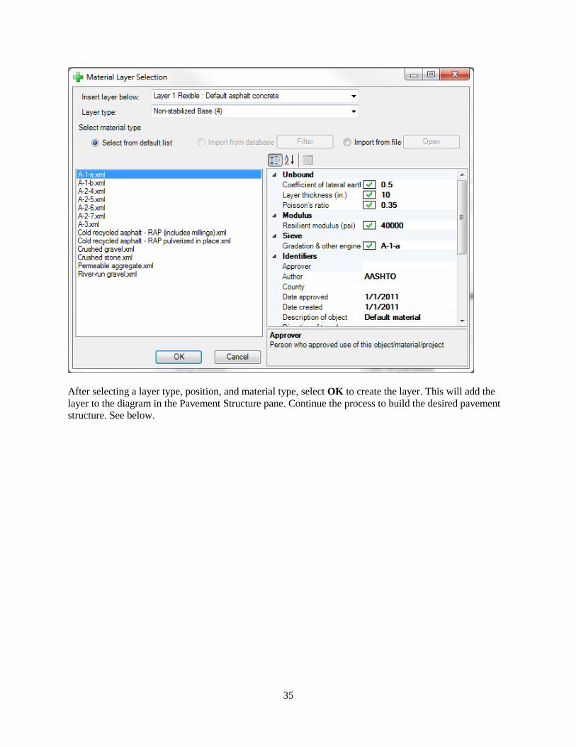
35

After selecting a layer type, position, and material type, select OK to create the layer. This will add the

layer to the diagram in the Pavement Structure pane. Continue the process to build the desired pavement

structure. See below.

36

5.4.1 Property Grid

Once the desired structure has been established, it is necessary to define layer-specific material inputs.

Open the asphalt concrete layer in the Property Grid by either left-clicking the layer in the Pavement

Structure pane or by selecting it from the Property Grid dropdown menu:

The Property Grid dropdown menu allows the user to select several input parameter sets, including layer

properties, project-specific calibration factors, and project identifiers. This example will focus on the

entry of layer properties which would be required for a new flexible pavement design.

37

Asphalt layer input parameters are shown in the figure above. Note that the dynamic modulus parameter,

which has been demonstrated to have significant impact on performance predictions (see Section 4 in this

document), requires different inputs at its different hierarchical input levels. At Level 1, MEPDG

dynamic modulus requires actual laboratory data at several temperatures and frequencies in order to

construct a master curve for the asphalt concrete. Levels 2 and 3 require only gradation test results for the

asphalt mixture.

38

Binder inputs are dependent on the input Level selection for asphalt dynamic modulus. At Levels 1 and 2,

ME Design requires binder properties in the form of laboratory test data for either binder grading system,

Superpave or Penetration/Viscosity Grade.

At Level 3 dynamic modulus, the user need only select (1) binder grading system and (2) binder grade.

Creep compliance inputs are also level-dependent. At Level 1, laboratory test results are required at

temperatures -4, 14, and 32°F. At Level 2, laboratory test results are only required at 14°F. At the lowest

level, ME Design internally calculates creep compliance at various temperatures and loading times based

on relationships with other inputs.

After entering surface layer data, continue through the Property Grid dropdown menu, defining the

necessary input data for each layer. See below for chemically stabilized, unbound base, and subgrade

layer properties.

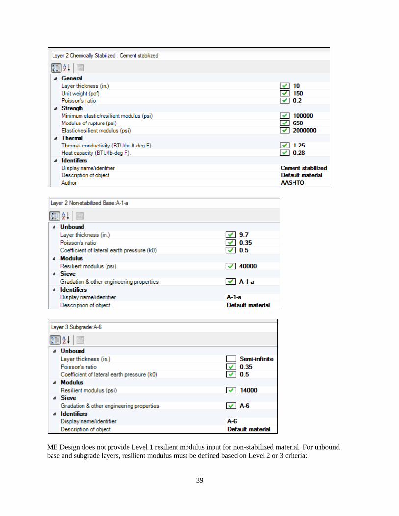
39

ME Design does not provide Level 1 resilient modulus input for non-stabilized material. For unbound

base and subgrade layers, resilient modulus must be defined based on Level 2 or 3 criteria:

40

At Level 2, resilient modulus can be defined directly or using correlations with other soil

properties. Level 2 input also supports the use of monthly average resilient modulus values. See

figure below.

At Level 3, default resilient modulus of the material can be overwritten manually.

5.5 Traffic

Traffic data in ME Design are accessed either by left-clicking the tire icon in the Pavement Structure

Definition area or via the Explorer tab > Project tree > Traffic node. This opens the Traffic tab, which

includes many of the traffic inputs described earlier in this document. These inputs can be divided into the

following general sections, as shown in the following figure.

Base Year Truck Volume and Speed

Traffic Capacity

Axle Configuration

Lateral Wander

Wheel Base

Vehicle Class Distribution

Axles Per Truck

Monthly Adjustment

Hourly Adjustment

Identifiers

41

Traffic capacity is an optional setting which allows a cap on forecasted traffic volume based on ME

Design’s internal Highway Capacity Manual (HCM) 2000 capacity calculations. This prevents

unrealistically high volumes from negatively impacting predicted pavement performance. The following

figure shows the capacity input dialog, which contains the necessary inputs for HCM calculations.

42

Vehicle class distribution can be defined with varying accuracy according to hierarchical input level. At

Level 3, predefined class distributions (or Truck Traffic Classification Groups) can be loaded from ME

Design which represent average values for a variety of selectable traffic stream types. See below. At

higher input levels, class distribution must be entered manually based on regional (Level 2) or local

(Level 1) values.

Axle load distributions are defined via a separate tab for each axle type: single, tandem, tridem and quad.

From the Explorer pane, open the Project tree > Traffic node and select the desired axle type to open the

associated Axle Load Distribution tab. These tabs contain axle load distribution factors, which represent

the total axle load applications within each load interval by vehicle class. Each axle type uses a separate

sheet. A single axle load distribution tab is shown below.

43

5.6 Climate

Climatic input parameters are accessible in two ways, similar to the Traffic tab:

1. From the Explorer tab, expand Project tree and double-left-click the Climate node, or

2. Left-click the white area (left of the tire) in the Pavement Structure Definition diagram.

The Climate tab contains all necessary climate inputs as outlined earlier in this document. These are

displayed below.

Average depth of water table can be defined on an annual or seasonal basis. This value is measured from

the top of subgrade surface to the ground water level. The view in the input entry window for this

parameter changes depending on the radio button selection. See below:

The Climate Station dialog allows two options for weather station selection. First, the user can choose a

single station from the list included in the station.dat file (stored by default in the

C:\...\AASHTOWare\ME Design\Defaults directory). Choosing a single station will also update latitude

and longitude fields accordingly.

44

Alternatively, a virtual weather station can be built by selecting multiple weather stations from the list.

This allows ME Design to build a composite set of weather conditions based on data from all the selected

sites. For each station, the Climate Station dialog displays distance from current project location (i.e.,

based on latitude/longitude), city, state, latitude and longitude, elevation, a brief description, and first and

last months of available data for that station. Climate data can be downloaded from the AASHTOWare

website (http://www.darwinme.org/MEDesign/ClimaticData.html) and loaded to the software by placing

the files in the C:\...\AASHTOWare\ME Design\HCD\ directory.

Once a weather station or virtual weather station is defined, the Summary tab displays a summary of

climatic input data, including annual and monthly average air temperature, annual precipitation, number

of wet days, freezing index, and average number of freeze/thaw cycles.

45

The Hourly Climate Data tab contains hourly data for the selected weather station. It is important to error-

check this data before attempting to run an analysis. Select the Verify Weather button to generate a list of

potential data errors in the Error List pane. These errors can include:

Missing or blank data

Data which are outside an acceptable range

The difference between the values of two consecutive hourly records is outside an acceptable

range

Any listed errors must be resolved by changing the offending values before ME Design can run analysis.

5.7 Analysis

Once inputs are completed, it is time to run analysis. To begin a model run, from the Menu toolbar select

Run. If a batch run is desired, select Batch Run.

During a model run, the Progress pane will display the status of any currently running analyses. Each step

in the model run process will be appear next to a color-coded status icon:

Green circle: The analysis is complete

Yellow triangle: The analysis is in progress

Red square: The analysis has not yet been run

To terminate analysis at any point, select Stop All Analysis from the Progress pane

Analysis steps are logged, with timestamps, in the Output pane.

46

5.8 Reporting

After completing an analysis run or batch run, a PDF report containing an input summary and output

reports will appear. This report is saved to the project directory (i.e., where the project *.dgpx file is

saved) and can also be accessed via the PDF Output Report item in the project tree of the Explorer pane.

The report is also available in Excel format if the corresponding option has been selected. To generate

Excel reports, go to the Explorer Pane > Tools > Options to open the Options tab. In the tab, set Generate

Excel Reports to True. After running analysis, select the item Excel Output Report in the project tree of

the Explorer Pane.

5.9 Optimization

ME Design includes an Optimization feature that allows the user to optimize the thickness of any one

layer at a time, in 0.5 inch increments, between user-defined minimum and maximum thicknesses. To

access the Optimization tab, go to the Explorer pane, expand the Project tree, and double-left-click the

Optimization node.

To perform optimization, select a layer in the Use column of the Design Layers field and define minimum

and maximum thicknesses. Then select the Optimize Thickness button at the bottom of the tab to run the

optimization process. ME Design displays the results of the optimization process in real time. When the

process has completed, the lowest satisfactory thickness will be displayed in the Last Optimized

Thickness field.

47

6. RECOMMENDATIONS FOR FUTURE RESEARCH

This document introduces the Mechanistic-Empirical Pavement Design Guide, including its conceptual

framework and methodology. It compares the design guide with the other major pavement design guide,

AASHTO’s Guide for Design of Pavement Structures, 1993 edition. It also introduces considerations

relevant for agencies considering implementation, including local calibration and sensitivity analysis.

Future research will continue to focus on factors relevant to a potential North Dakota MEPDG

implementation. First, MEPDG transfer functions must be locally calibrated using North Dakota

historical distress data. Local calibration is an important step toward implementation, which was

discussed above in detail. A calibrated set of MEPDG distress functions must be achieved before any

further investigations of region-specific MEPDG behavior can occur.

Local calibration requires agencies to initially select hierarchical input level for each parameter based on

the understanding that higher level inputs generally contribute to more accurate pavement performance

predictions. However, relatively little literature exists to quantify the expected impact of input level on

model accuracy. This information could be useful to an agency interested in the most cost-effective

implementation and data collection plan.

The move toward MEPDG implementation is predicated on the understanding that MEPDG yields more

cost-effective pavement structures than the 1993 AASHTO method does. Many agencies, however, have

been interested in testing this assertion under local material, traffic, climate, and policy conditions. A

comparison between the 1993 AASHTO empirical model and a locally calibrated set of MEPDG

performance models could either confirm or cast doubt on the usefulness of the new design method on

North Dakota roads. Cost-effective pavement design is, of course, of particular interest to the oil-

impacted region of western North Dakota.

While MEPDG is a more theoretically sound pavement design procedure than the AASHTO method, its

implementation must ultimately offer long-term financial benefits to each adopting agency in terms of

better pavement designs. It is not enough, particularly in the current climate of shrinking financial

resources, for a pavement design procedure to be solely based on sound engineering principles. The

method must be demonstrated to be cost-effective in implementation and in practice. The research needs

identified above will help satisfy these needs for the state of North Dakota.

48

REFERENCES

ARA. Applied Research Associates Inc. Guide for Mechanistic-Empirical Design of New and

Rehabilitated Pavement Structures (NCHRP 1-37A report). ERES Consultants Division, Champaign, IL,

2004.

AASHTO. 1972. AASHTO Interim Guide for Design of Pavement Structure. Washington, DC.

AASHTO. 1986. AASHTO Guide for Design of Pavement Structures. Washington, DC.

AASHTO. 1993. AASHTO Guide for Design of Pavement Structures. Washington, DC.

Banerjee, A., J. Pablo, A.F. Smit, and J.A. Prozzi. 2008. Development of the Texas Flexible Pavements

Database. FHWA/TX-10/0-5513-2. Texas DOT, Austin, TX.

Ceylan, H., S. Kim, K. Gopalakrishnan, and D. Ma. 2013. Iowa Calibration of MEPDG Performance

Prediction Models. InTrans Project 11-401, TS13-002. Ames, IA.

Darter, M.I., L. Titus-Glover, and H.L. Von. (2009). Implementation of the Mechanistic-Empirical

Pavement Design Guide in Utah: Validation, Calibration, and Development of the UDOT MEPDG User’s

Guide. UT-09.11. UDOT, Salt Lake City, UT.

FHWA. 2007. Updates on Mechanistic Empirical Pavement Design Guide (MEPDG).

http://www.google.com/url?sa=t&rct=j&q=mepdg+implementation+states+survey&source=web&cd=2&

cad=rja&ved=0CDgQFjAB&url=http%3A%2F%2Fitd.idaho.gov%2Fpdc09%2Fpresentations%2FMEPD

G%2520Update%2520-

%2520tyu.ppt&ei=gPZ6UYH8AcS_qgHrx4HIBA&usg=AFQjCNE7e10_g8g9NDoDoLRCN52iukVy2w

&bvm=bv.45645796,d.b2I. access: April. 15, 2013.

Hall, K.D., D.X. Xiao, and K.C.P. Wang. 2011. Calibration of the MEPDG for Flexible Pavement Design

in Arkansas. Transportation Research Board 2011 Annual Meeting Proceeding, Washington, DC.

Highway Research Board (HRB) 1961. The AASHO Road Test: Report 1, Highway and Description of

the Project (Special Report 61A). National Academy of Sciences, Washington, DC.

Kang, M. and T. Adams. 2007. Local Calibration for Fatigue Cracking Models used in the Mechanistic-

Empirical Pavement Design Guide. Proceedings of the 2007 Mid-Continent Transportation Research

Symposium, Ames, IA, August 2007.

Kim, Y.R., F.M. Jadoun, T. Hou, and N. Muthadi. 2011. Local Calibration of the MEPDG for Flexible

Pavement Design. HWY\NC\2007-07. NCDOT, Raleigh, NC.

Kim, S., H. Ceylan, K. Copalakrishan, O. Smadi, C. Brakke, and F. Behnami. (2010). Verification of

Mechanistic-Empirical Pavement Design Guide (MEPDG) Performance Predictions Using Pavement

Management Information System (PMIS). Transportation Research Board 2010 Annual Meeting, TRB

Paper 10-2395, p.20. Washington, DC.

Li, J., Uhlmeyer, J.S., Mahoney, J.P., and Muench, S.T., 2011. Use of the 1993 AASHTO Guide,

MEPDG and Historical Performance to Update the WSDOT Pavement Design Catalog, report no. WA-

RD 779.1, the state of Washington DOT.

49

Li, Q., D. Xiao, K. Wang, K. Hall, and Y. Qiu. 2011, Mechanistic-empirical pavement design guide

(MEPDG): a bird’s-eye view, Journal of Modern Transportation, V.19, P. 114-133

NCHRP. 2004. Design of New and Rehabilitated Pavement Structures. NCHRP Study 1-37A. National

Cooperative Highway Research Program. Washington DC, July 2004.

Schroer, J. 2012. Local Calibration of the MEPDG for HMA Pavement in Missouri. Proceedings of the

2012 NCAUPG annual meeting, Indianapolis, IN, February 2012.

Schwartz, C.W. and R.L. Carvalho. Implementation of the NCHRP 1-37A Design Guide Final Report

Volume 2: Evaluation of Mechanistic-Empirical Design Procedure. MDSHA Project No. SP0077B41,

Maryland State Highway Administration, Lutherville, MD, 2007.

Tarefder, R.A., N. Sumee, J.I. Rodriguez, S. Abbina, and K. Benedict. 2012. Development of a flexible

pavement database for local calibration of MEPDG. NM08MSC-02. New Mexico DOT, Albuquerque,

NM.

Velasquez, R., K. Hoegh, I. Yut, N. Funk, G. Cochran, M. Marasteanu, and L. Khazanovich. (2009).

Implementation of the MEPDG for New and Rehabilitated Pavement Structures for Design of Concrete

and Asphalt Pavement in Minnesota. MN/RC 2009-06. MnDOT, Minneapolis, MN.

Zhang, Z., J.P. Leidy, I. Kawa, and W.R. Hudson. 2000. “Impact of Changing Traffic Characteristics and

Environmental Conditions on Flexible Pavement.” Transportation Research Record No. 1730,

Washington, DC, 2000, pp. 125-131.

Zhou, C., B. Huang, X. Shu, and Q. Dong. (2013). Validating MEPDG with Tennessee Pavement

Performance Data. Journal of Transportation Engineering. 2013.139:306-312.

Quintus, H.L. and J.S. Moulthrop. 2007. Mechanistic-Empirical Pavement Design Guide Flexible

Pavement Performance Prediction Models for Montana. FHWA/MT-07-008/8158-1.

NCHRP, 2010. Guide for the Local Calibration of the Mechanistic-Empirical Pavement Design.

Aguiar-Moya, J.P., Banerjee, A., and Prozzi, J.A. (2009). “Sensitivity analysis of the MEPDG using

measured probability distributions of pavement layer thickness,” Annual Meeting of Transportation

Research Board (CD-ROM), National Research Council, Washington, DC

(http://pubsindex.trb.org/view.aspx?id=880657)

Ahn, S., Kandala, S., Uzan, J., and El-Basyouny, M. (2009). “Comparative Analysis of Input Traffic Data

and MEPDG Output for Flexible Pavements in State of Arizona,” Annual Meeting of Transportation

Research Board (CD-ROM), National Research Council, Washington, DC

(http://pubsindex.trb.org/view.aspx?id=881969)

Ayyala, D., Chehab, G. R., and Daniel, J. S. (2010). “Sensitivity of MEPDG Level 2 and 3 Inputs using

Statistical Analysis Techniques for New England States,” Annual Meetings of the Transportation

Research Board (CD-ROM), National Research Council, Washington DC, Paper 10- 3694.

50

Buch, N., Chatti, K., Haider, S. W., and Manik, A. (2008). “Evaluation of the 1-37A Design Process for

New and Rehabilitated JPCP and HMA Pavements,” Research Report RC-1516, Michigan State

University, East Lansing, MI; June.

Buch, N., Chatti, K., Haider, S., Baladi, G., Brink, W., and Harsini, I. (2013). “Preparation for

Implementation of the Mechanistic-Empirical Pavement Design Guide in Michigan Part 2: Evaluation of

Rehabilitation Fixes. Final Report,” Research Report RC-1594, Michigan State University, East Lansing,

MI.

Darter, M. I., Khazanovich, L., Witczak, M., and Zapata, C. (2006). NCHRP Research Results Digest

308: Changes to the Mechanistic-Empirical Pavement Design Guide Software Through Version 0.900.

Transportation Research Board, National Research Council, Washington, DC.

(http://www.trb.org/news/blurb_detail.asp?id=7070) [Versions 0.7/0.8/0.9]

Hall, K. D., Xiao, X. D., and Wang, K. C. P. (2010). “Thickness Estimation of Existing Pavements Using

Nondestructive Techniques: Matching Accuracy to Application,” Annual Meeting of Transportation

Research Board (CD-ROM), National Research Council, Washington, DC.

Hoerner, T. E., Zimmerman, K. A., Smith, K. D., and Cooley, L. A. (2007). Mechanistic-Empirical

Pavement Design Guide Implementation Plan, Report No. SD2005-01, South Dakota Department of

Transportation, Pierre, SD.

Khazanovich. L., Wojtkiewicz. S. F. and Velasquez. R. (2008). “MEPDG-RED: A Framework for

Reliability Analysis with the Mechanistic-Empirical Pavement Design Procedure,” Transportation

Research Board 87th Annual Meeting, Washington DC.

Kim, Y. R., King, M., and Momen, M. (2005). “Typical Dynamic Moduli for North Carolina Asphalt

Concrete Mixes.” Research Report FHWA/NC/2005-03, North Carolina Department of Transportation,

Raleigh, NC.

Kim, Y., Im, S., and Ban, H. (2010). “Layer Moduli of Nebraska Pavements for the New Mechanistic-

Empirical Pavement Design Guide (MEPDG),” Research Report MPM-08, University of Nebraska-

Lincoln, Lincoln, NE.

McCracken, J. K., Vandenbossche J.M., and Asbahan, R.E. (2008). “Effect of the MEPDG Hierarchal

Levels on the Predicted Performance of a Jointed Plain Concrete Pavement,” Proc., 9th International

Conference on Concrete Pavements, San Francisco, CA.

National Cooperative Highway Research Program (2004). Guide for Mechanistic-Empirical Design of

New and Rehabilitated Pavement Structures. Final Report, NCHRP Project 1-37A, Transportation

Research Board, National Research Council, Washington, DC

Schwartz, C. W. (2009). “Influence of Unbound Materials on Flexible Pavement Performance: A

Comparison of the AASHTO and MEPDG Methods,” Eighth International Conference on the Bearing

Capacity of Roads, Railways, and Airfields, Urbana-Champaign IL, July, p. 951 – 959.

Schwartz, C. W. and Li, R., (2010). “Sensitivity of Predicted Flexible Pavement Performance to Unbound

Material Hydraulic Properties,” Advances in Analysis, Modeling, and Design (GeoFlorida 2010),

American Society of Civil Engineers, Reston, VA.

51

Schwartz, C.W. and Carvalho, R.L. (2006). “Implementation of the NCHRP 1-37A Design Guide, Final

Report Volume 2: Evaluation of Mechanistic-Empirical Design Procedure,” MDSHA Project No.

SP0077B41, Maryland State Highway Administration, Lutherville, MD.

Schwartz, C.W., Li, R., Kim, S., Ceylan, H., and Gopalakrishnan, K. (2011). Sensitivity Evaluation of

MEPDG Performance Prediction. Final Report, NCHRP Project 1-47, University of Maryland, College

Park, MD.

Thyagarajan, S., Sivaneswaran, N., Muhunthan, B., and Petros, K. (2010). “Statistical Analysis of Critical

Input Parameters in Mechanistic Empirical Pavement Design Guide,” Journal of the Association of

Asphalt Paving Technologists, Vol. 79, p. 635-662. Asphalt Paving Technology 2010, Sacramento, CA,

March 7-10.

Velasquez, R., Hoegh, K., Yut, I., Funk, N., Cochran, G., Marasteanu, M. O., and Khazanovich, L.

(2009). “Implementation of the MEPDG for New and Rehabilitated Pavement Structures for Design of

Concrete and Asphalt Pavements in Minnesota,” Research Report Mn/DOT 2009-06, University of

Minnesota, Minneapolis, Minnesota, January.

Yin, H., Chehab, G. R., Stoffels, S. M., Kumar, T., and Premkumar, L. (2010). “Use of Creep

Compliance Interconverted from Complex Modulus for Thermal Cracking Prediction Using the M-E

Pavement Design Guide,” International Journal of Pavement Engineering, Vol. 11, No. 2, April, p. 95-

105.

ILLI-PAVE PC Version User’s Manual (1990). NCHRP Project 1-26, Transportation Facilities Group,

University of Illinois, Urbana-Champaign, IL.

Ayres, M. and M. Witczak. (1998). “AYMA – A Mechanistic Probabilistic System to Evaluate Flexible

Pavement Performance,” Transportation Research Board 77th Annual Meeting, Paper No. 980738,

Washington, DC.

Carey, W.N. and P.E. Irick (1990). The Pavement Serviceability-Performance Concept. Highway

Research Bulletin 250. Washington, DC: Highway Research Board.

AASHTO (2008). Mechanistic-Empirical Pavement Design Guide: A Manual of Practice, AASHTO,

Washington, DC.

Ceylan, M., Kim, S., Gopalakrishnan, K. and D. Ma. (2013). Iowa Calibration of MEPDG Performance

Prediction Models. Iowa State University, Ames, IA.

Pierce, L., K. Zimmerman, and N. Saadatmand. (2011). Use of Pavement Management Data for

Calibration of the Mechanistic-Empirical Pavement Design Guide, unpublished report

Hudson, W.R., W. Visser, C. Monismith, C. Dougan. (2008). “Using State PMS Data to Validate the New

Mechanistic/Empirical Pavement Design Guide (MEPDG),” Seventh International Conference on

Managing Pavement Assets, Washington, DC.

Williams, C. and R. Shaidur. (2013). Mechanistic-Empirical Pavement Design Guide Calibration for

Pavement Rehabilitation. Iowa State University, Ames, IA.

52

Federal Highway Administration (2010). “Local Calibration of the MEPDG Using Pavement

Management Systems,” FHWA-HIF-11-026, Federal Highway Administration, Washington, DC.