North Atlantic Mesoscale Eddy Detection and Marine Species

1

North Atlantic Mesoscale Eddy Detection and Marine Species Distribution

by

Ango Chen-Tien Hsu

Date: May 2010

Approved:

_______________________________________

Patrick N. Halpin, Advisor

Masters project submitted in partial fulfillment of the requirements for

the Master of Environmental Management degree in

the Nicholas School of the Environment of

Duke University

2

ABSTRACT

An eddy detection workflow was developed and applied to reference series of delayed

time maps of sea level anomaly (Ref DT-MSLA) published by Aviso Altimetry, France

in the North Atlantic region between 30-55° N and 30-80° W. The eddy detection

parameters, maximum/minimum Okubo-Weiss parameter to assign to the eddy core/ring,

minimum eddy core area, minimum eddy core area to perimeter ratio, and minimum eddy

duration, were set to -0.2/0.2 standard deviation, 5 cells (6869 km2), 0.4, and 10 images

(70 days), respectively. Using these parameters, 635 anticyclonic eddies and 930 cyclonic

eddies were detected between October 14, 1992 and December 31, 2005. The eddy

structure of the 62103 pelagic longline fishery catch records in The Logbook System

maintained by Southeast Fisheries Science Center was sampled. One-way ANOVA and t-

test were conducted to compare the mean catch-per-unit-effort (CPUE) of bluefin tuna

(Thunnus thynnus), yellowfin tuna (Thunnus albacores), bigeye tuna (Thunnus obesus),

and swordfish (Xiphius gladius) at different eddy structures. For bluefin tuna and bigeye

tuna, the mean CPUE is higher in the eddy area than in the non-eddy area. For yellowfin

tuna and swordfish, the mean CPUE is higher in the non-eddy area than in the eddy area.

For all three species of tuna, the mean CPUE is higher in the anticyclonic eddies than in

the cyclonic eddies. For swordfish, the mean CPUE is higher in the cyclonic eddies than

in the anticyclonic eddies. The results suggest different eddy structures make different

habitats for large marine predators and eddy activities contribute to marine species

distribution.

3

ACKNOWLEDGEMENT

The project would not have succeeded without the extensive support and help I received

from many people. My thanks to all of you and to those I forgot to mention. Thanks to Dr.

Pat Halpin, my research advisor, for supporting this project, introducing me to the world

of GIS, and many opportunities he offered in the past two years. I learned a lot through

those opportunities and I feel that somehow changed my life. Thanks to Jason Roberts for

spending countless hours talking to me on Skype and patiently teaching me all kinds of

knowledge in remotely sensed oceanographic data, different software packages, and

programming in the past two years. Jason is a significant part of my Nicholas School

experience. Thanks to Dr. Andre Boustany for sharing the fishery catch data and his

knowledge in marine biology. Thanks to Dr. Paul Baker, my academic advisor, for being

in charge of me since the first day I switched to GEC which is my second day at the

Nicholas School. Thanks to Dr. Susan Lozier for a great class in fluid dynamics which

helped the progress of this project. Thanks to John Fay for his help in geoprocessing

scripts using Python. Thanks to all my colleagues and friends and administrative staffs in

the Nicholas School for making me two great years. Thanks to Janice for her

encouragement and the happiness she brings to my life. A special thank to my family,

especially my parents, for their nonstop support, both financial and spiritual. They are, to

most extent, the most important part of my life.

4

Table of Contents

Abstract……………………………………………………………...……………………2

Acknowledgement……..….…………………………………………...…………………3

Introduction……………………………………………………………………………....5

Methods…………………………………………………………………………………...9

Sea Level Anomaly Maps……...………….……………………………………….…9

Eddy Detection………………………...……………………………………………11

Pelagic Longline Fishery Catch Data....…………………………………...………..14

Sampling...………………………………………...…………………………...……16

Analysis…………………………...…………………..…………………………….17

Results and Discussion…………………………………………………………….……18

Eddy Detection…………………..,…………………………………………...……18

Sampling…………………………………………………………………………....19

Marine Species Distribution…………………………………………….………….20

Future Research…………………………………………………………….………26

Literature Cited………………………………………...………………………………27

5

Introduction

Eddies, or vortices, are nonlinear ocean mesoscale (scales of tens to hundreds of

kilometers and tens to hundreds of days) variability. At the eddy center, the eddy core,

vorticity dominates. The eddy ring, which surrounds the eddy core, experiences high rate

of strain. According to oceanographers, eddy core is often comprises 50% to 60%

diameter of the entire eddy (Henson and Thomas 2008). Eddies occur in every ocean on

Earth, including Arctic and Antarctic regions. Mesoscale eddies occur when there is a

balance between two major forces, horizontal pressure gradient force arising from

differences in water density and the Coriolis force associated with the Earth’s rotation

(University of Hawaii website, www.geol.sc.edu/cbnelson/Eddy/index.htm). Other eddy

formation mechanisms include currents moving vertically or flowing over seamounts,

Rossby waves which travel westward over planetary scale, and spatial variation of water

temperature. In the study area of this project, the North Atlantic region, the flow

instabilities of the Gulf Stream pinches off relatively warm or cool waters that act as

seeds for eddies. Eddies are generated at both sides of the current as the filaments of the

current deform. Convergence and divergence of upper ocean waters produced by winds

can also create eddies. The diameters of eddies vary from a few centimeters to hundreds

of kilometers. Some eddies disappear soon after its generation while some can last

months to years. Depending on the direction of rotation, eddy has two polarities,

anticyclonic and cyclonic. In the northern hemisphere, anticyclonic eddy rotate clockwise

and cyclonic eddy rotates counter-clockwise. The rotation directions of both anticyclonic

eddy and cyclonic eddy reverse in the southern hemisphere. For both anticyclonic eddy

and cyclonic eddy, centrifugal force points outward. The Coriolis force, which usually

6

outweighs centrifugal force, points inward in the anticyclonic eddy and outward in the

cyclonic eddy. In the anticyclonic eddy, excess inward directed force drives water toward

the interior of the eddy, increases the hydrostatic pressure, and creates downwelling at the

eddy core. The eddy core of anticyclonic eddy appears as clustered positive cells on sea

level anomaly maps since high hydrostatic pressure is created. We refer anticyclonic

eddy as the warm ring because its downwelling at the eddy core which often traps warm

water. In contrast, in the cyclonic eddy, excess outward directed force drives water

outward the interior of the eddy, decreases the hydrostatic pressure, and forces the eddy

core to upwell. The eddy core of cyclonic appears as clustered negative cells on sea level

anomaly maps since low hydrostatic pressure is created. We refer cyclonic eddy as the

cold ring because it upwells at the eddy core and brings relatively cool water from bottom

of the ocean. The downwelling and upwelling characteristics at the eddy core of

anticyclonic eddy (warm ring) and cyclonic eddy (cold ring) apply to both hemispheres

(Bakun 2006).

The kinetic energy of mesoscale variability is more than an order of magnitude greater

than the mean kinetic energy over most of the ocean (Wyrtki et al. 1976; Richardson

1983). Eddies are rotating water masses that contribute to the general circulation,

large-scale water mass distributions, and ocean biology because of their effectiveness in

transporting momentum, heat, mass, chemical constituents, and nutrients and their impact

on mixing (Olson 1991; Chelton et al. 2007). At the center of a cyclonic eddy, freshly

upwelled cool, nutrient-rich waters are a feast for phytoplankton. On the other hand, the

anticyclonic eddy draws and aggregates water and materials from the ambient

environment to form a highly concentrated area of these materials at its center. Many

7

research had shown that eddy activities affect water temperature (Gasca 2003a), nutrient

cycling (McGillicuddy et al. 2003), phytoplankton and zooplankton assemblage (Paterson

et al. 2007), the distribution and abundance of hyperiid amphipods (Gasca 2003b),

sardine larvae survival (Logerwell et al. 2001), and fish distribution (Brandt 1981). The

above facts led me to assume eddy activities affect the distribution of large predators in

the marine ecosystem and these predators consider different eddy structures (eddy core;

eddy ring) and different eddy polarities (anticyclonic eddy; cyclonic eddy) different

habitats.

The project has two objectives. The first objective is to develop a workflow to detect

eddy structures on time series sea level anomaly maps with the help of software packages

such as Matlab, ArcGIS, and Python. An existing eddy core detection tool was applied in

the North Atlantic region looking for eddy cores on 14 year (Oct. 1992 to Dec. 2005)

time series sea level anomaly maps. The detected eddy cores were then buffered

proportionally and eddy rings were searched within the buffer with a Python script that I

composed. The second objective is to determine if eddy activities affect marine species

distribution. I analyze a pelagic longline fishery catch dataset presented in The Logbook

System with the detected eddy structures. I calculated catch-per-unit-effort (CPUE) of

four large marine predator species, bluefin tuna (Thunnus thynnus), yellowfin tuna

(Thunnus albacores), bigeye tuna (Thunnus obesus), and swordfish (Xiphius gladius), by

dividing the number of fish caught of each species by the number of hook set at each

catch point and conducted one-way ANOVA and t-test to compare if mean CPUE of each

species is significantly different at different eddy structures or at eddy structure with

different polarities. In this project, I focused on eddies which have a diameter of hundreds

8

of kilometers and last for months because those small and short lived eddies are not likely

to be important to marine species distribution.

9

Methods

Sea Level Anomaly Maps

The remotely sensed dataset I worked with to detect eddies is delayed time map of sea

level anomaly (DT-MSLA) published by Aviso Altimetry, France. The Doris System

accurately tracks the position of an altimetry satellite based on the Doppler Effect. With

position information of the satellite, the height of the satellite to a reference ellipsoid can

be determined. By transmitting radar pulse to earth and measuring satellite-to-surface

round-trip time of the pulse, the distance between satellite and sea surface is calculated.

Sea surface height is derived by subtracting the distance between satellite and sea surface

from height of the satellite. The dataset is accurate to a degree of a few centimeters. The

dataset is ongoing and the earliest data goes back to September 1992. The spatial

resolution and time resolution of the dataset are 37 kilometers and 7 days, respectively.

For every seven days, we have a gridded sea level anomaly computed with respect to a

seven-year mean covering the entire globe. DT-MSLA sea level anomalies have two sub-

datasets, reference series (Ref) and updated series (Upd). I worked with reference series

sub-dataset since it always averages measurements of two satellites with the same ground

track, hence the reference series sub-dataset set is homogeneous through time. Depending

on different time periods, the two satellites could be Topex/Poseidon/ERS, Jason-

1/Envisat, or Jason-2/Envisat. In contrast, update series keeps adding measurements of up

to four different satellites whenever a new satellite becomes available. Although update

series provides more and more accurate measurements with increased satellite number, it

would give non-homogeneous information of sea level anomaly throughout the images I

detect eddy structures on. One advantage of sea level anomaly maps is radar pulse isn’t

10

affected by clouds. I needn’t to deal with clouds in this project since there won’t be cloud

contamination on the satellite images.

I downloaded reference series delayed time map of sea level anomaly (Ref DT-MSLA)

between October 1992 and December 2005, clipped the downloaded images to an extent

of the study area, the North Atlantic region between 30-55° N and 30-80° W, and fed the

clipped images as the inputs of the workflow of detecting eddy structures on time series

sea level anomaly maps. Figure 1 is an example of global extent sea level anomaly map

on January 3rd

, 2007. The black box on the figure depicts the extent of the study area.

Figure 2 is the same image clipped to the North Atlantic region which has the extent

within which I detected eddies in this project. Both images are in a Mercator projection

with geographic coordinate system, datum, and spheroid defined by Aviso Altimetry.

Figure 1. Global extent sea level anomaly map on January 3rd

, 2007. The black box on

the figure depicts the extent of the study area, the North Atlantic region.

11

Figure 2. The same image as Figure 1 clipped to the extent of the study area, the North

Atlantic region.

Eddy Detection

The Okubo-Weiss parameter, W, is often used to identify eddies in two-dimension sea

level anomaly maps. The Okubo-Weiss parameter is defined as the normal component of

strain (sn2) plus the shear component of strain (ss

2) minus vorticity (ω

2), W = sn

2 ＋ ss

2 －

ω2. Dominated by vorticity, eddy core has large negative Okubo-Weiss parameter. In

contrast, eddy ring, which is dominated by strain, has large positive Okubo-Weiss

parameter. Henson and Thomas (2008) showed this relationship between eddy core, eddy

ring, and the Okubo-Weiss parameter with a transect which runs through a mesoscale

marine eddy (Figure 3; Henson and Thomas 2008).

12

Figure 3. Plot of a transect which runs through an eddy against the Okubo-Weiss

parameter (solid line in the right panel). The plot shows the eddy core has large negative

Okubo-Weiss parameter while the eddy ring has the large positive Okubo-Weiss

parameter.

Along with some other 200 tools, an existing eddy core detection tool is contained in

Marine Geospatial Ecology Tools (MGET). Also known as GeoEco python package,

MGET is an open source geoprocessing toolbox designed for coastal and marine

researchers and GIS analysts who work with spatially-explicit ecological and

oceanographic data (Roberts et al.). The eddy core detection tool MGET contains is a

Matlab code which is able to detect eddy cores on time series sea level anomaly maps.

Current eddy core detection tool walks through a few steps on sea level anomaly maps

before it is able to compute the Okubo-Weiss parameter and assign cells with large

negative Okubo-Weiss parameter to eddy core. It starts with deriving the u component

and the v component of the velocity field from sea level anomalies based on two

equations, and , in which is sea level anomaly, is acceleration

due to gravity, and is Coriolis parameter. The tool further computes the normal

component and the shear component of strain and vorticity from the u component and the

13

v component of the velocity field with the following equations: sn = ∂xu － ∂yv, ss = ∂xv

＋ ∂yu, and ω = ∂xv － ∂yu, to calculate the Okubo-Weiss parameter. Scientists have not

reached a consensus on the threshold Okubo-Weiss parameter to assign to the eddy core

and the eddy ring in the eddy identification research. Some oceanographers set maximum

Okubo-Weiss parameter to 0.2σω to assign to the eddy core, where σω is the spatial

standard deviation of the Okubo-Weiss parameter (Isern-Fontanet et al. 2006). Henson

and Thomas set maximum Okubo-Weiss parameter to 0.2σω to assign to the eddy core

as well as minimum Okubo-Weiss parameter to 0.2σω to assign to the eddy ring (Henson

and Thomas 2008). Chelton et al. (2007) picked -2*10-12

s-2

as maximum Okubo-Weiss

parameter to assign to the eddy core (Chelton et al. 2007). In this project, I set maximum

Okubo-Weiss parameter to 0.2σω to assign to the eddy core and minimum Okubo-Weiss

parameter to 0.2σω to assign to the eddy ring.

Other than the maximum Okubo-Weiss parameter to assign to the eddy core, the eddy

core detection tool takes another three input parameters, minimum eddy core area,

minimum eddy core area to perimeter ratio (scaled such that perfect circular has a value

of 1.0), and minimum eddy duration. To detect large, long lived eddies (hundreds of

kilometers in diameter, lasting for months) which are likely to be important to marine

species distribution, I tried different combinations of input parameters and compared the

detected eddy cores to sea surface temperature images prepared by GOES 11 Satellite

and GOES 12 Satellite to make sure the eddy core detection tool captures most of the

eddy-like structures on the sea surface temperature images. I set the thresholds listed in

Table 1 for the tool’s input parameters to detect eddy cores in the North Atlantic region.

14

Table 1. Thresholds for input parameters set in the eddy core detection tool.

Tool input parameter Threshold

Maximum Okubo-Weiss parameter to assign to eddy core 0.2σω

Minimum eddy core area 5 cells = 6869 km2

Minimum eddy core area to perimeter ratio 0.4

Minimum eddy duration 10 images = 70 days

The tool outputs detected eddy cores with metadata such as the polarity, whether the

detected eddy cores are anticyclonic eddies or cyclonic eddies, and the age of the

detected eddy cores on a particular image.

With a Python script that I composed, I buffered the detected eddy cores proportionally

so the detected eddy cores comprise roughly 50% diameter of the buffers and search large

positive Okubo-Weiss parameter, 0.2σω, within the buffers to assign to the eddy ring. At

the end of the eddy detection process, for every 7 days, I have polygon layers of

anticyclonic eddy core, cyclonic eddy core, anticyclonic eddy ring, and cyclonic eddy

ring that I used the catch points presented in the pelagic longline fishery catch dataset to

sample with.

Pelagic Longline Fishery Catch Data

The pelagic longline fishery catch data I worked with is presented in The Logbook

System and maintained by Southeast Fisheries Science Center. The data is ongoing and

goes back to 1992. I used the data between October 1992 and December 2005 to match

the start date of the sea level anomaly dataset. The data after 2005 of the fishery data

hasn’t been processed and cleaned, hence is hard to work with. The fishery catch data has

some 160,000 catch points in between October 1992 and December 2005. After parsing

out all the catch points which are outside the study area, the North Atlantic region

between 30-55° N and 30-80° W, I was left with 62,121 catch points (Figure 4). At every

15

catch point, I have information of date, location (latitude and longitude), number of fish

caught of each species, and number of hooks set. Table 2 is an example of a few rows of

the fishery data. At each catch point, I calculated catch-per-unit-effort (CPUE) of each

species by dividing the number of fish caught of each species by the number of hooks set.

The reason that I must normalize number of fish caught by the number of hooks and

analyze mean CPUE of each species with respect to different eddy structures is, if I see a

high mean CPUE of a species at a particular eddy structure, I wouldn’t know it’s because

of the eddy activities or it’s because there is more fishing in the area.

Figure 4. The 62,121 catch points presented in The Logbook System within the study

area, the North Atlantic region.

16

Table 2. A few rows of the fishery catch data. At every catch point, I have information of

date, latitude, longitude, number of swordfish (SWO), bigeye tuna (BET), bluefin tuna

(BFT), and yellowfin tuna (YFT) caught, and number of hooks set.

Sampling

I sampled the distances each catch point to anticyclonic eddy core, to cyclonic eddy core,

to anticyclonic eddy ring, and to cyclonic eddy ring with the help of the “Find Nearest

Features Listed in Field” tool presented in MGET. I then determined the distance each

catch point to eddy core by looking at the minimum distance between distance to

anticyclonic eddy core and distance to cyclonic eddy core. Similarly, I determined the

distance each catch point to eddy ring by looking at the minimum distance between

distance to anticyclonic eddy ring and distance to cyclonic eddy ring. Finally I

determined what eddy structure each catch point locates based on the information of

these distances each catch point to different eddy structures that I sampled. Table 3 is a

fictitious table which illustrates the sampling process.

17

Table 3. A fictitious table which illustrates the sampling process. Distance to anticyclonic

eddy core (column M), to cyclonic eddy core (column N), to anticyclonic eddy ring

(column O), to cyclonic eddy ring (column P) of each catch point were sampled. Distance

of each catch point to eddy core (column Q) is determined by looking at the minimum

between column M and N and distance of each catch point to eddy ring (column R) is

determined by looking at the minimum between column O and P. Finally, which eddy

structure each catch point locates was categorized.

Analysis

I compared the mean CPUE of the four marine species, bluefin tuna, yellowfin tuna,

bigeye tuna, and swordfish, at different eddy structures and at eddy structure with

different polarities. When more than two groups are involved, one-way ANOVA was

conducted followed by a Bonferroni test to determine the mean CPUE of which two

groups are significantly different at 95% confidence level. When the comparison involves

only two groups, t-test was conducted.

18

Results and Discussion

Eddy Detection

With the input parameters of the eddy detection workflow setting to the thresholds

described in the Methods session, 1565 eddy cores were detected between October 1992

and December 2005 in the North Atlantic region. Among which, 635 detected eddy cores

are anticyclonic eddy cores and 930 detected eddy cores are cyclonic eddy cores. The

eddy which has the longest duration survives 81 images (567 days). The image which has

the most detected eddy cores has 47 detected eddy cores. Figure 5 is an example of

detected eddy cores. All the detected anticyclonic eddy cores locate within the area of

large positive sea level anomaly and all the detected cyclonic eddy cores locate within the

area of large negative sea level anomaly. When overlapping with the direction and

magnitude of the geostrophic current, clockwise rotation of the anticyclonic eddy core

and counter-clockwise rotation of the cyclonic eddy core were observed.

19

Figure 5. An example of detected eddy cores. Anticyclonic eddy cores locate within the

area of large positive sea level anomaly and all cyclonic eddy cores locate within the area

of large negative sea level anomaly. Anticyclonic eddy cores rotate clockwise and

cyclonic eddy cores rotate counter-clockwise.

Sampling

I categorized the 62,121 catch points to the eddy structure they locate by looking at the

information of their distances to different eddy structures that I sampled. 18 catch points

20

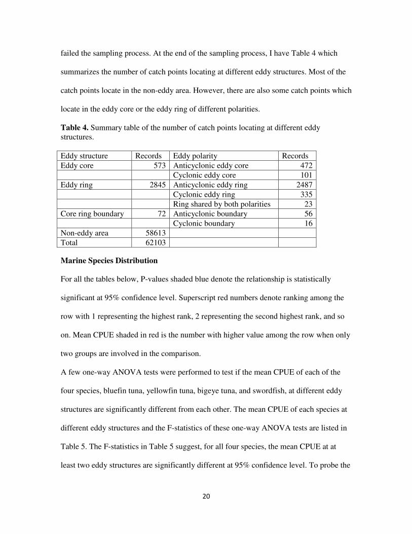
failed the sampling process. At the end of the sampling process, I have Table 4 which

summarizes the number of catch points locating at different eddy structures. Most of the

catch points locate in the non-eddy area. However, there are also some catch points which

locate in the eddy core or the eddy ring of different polarities.

Table 4. Summary table of the number of catch points locating at different eddy

structures.

Eddy structure Records Eddy polarity Records

Eddy core 573 Anticyclonic eddy core 472

Cyclonic eddy core 101

Eddy ring 2845 Anticyclonic eddy ring 2487

Cyclonic eddy ring 335

Ring shared by both polarities 23

Core ring boundary 72 Anticyclonic boundary 56

Cyclonic boundary 16

Non-eddy area 58613

Total 62103

Marine Species Distribution

For all the tables below, P-values shaded blue denote the relationship is statistically

significant at 95% confidence level. Superscript red numbers denote ranking among the

row with 1 representing the highest rank, 2 representing the second highest rank, and so

on. Mean CPUE shaded in red is the number with higher value among the row when only

two groups are involved in the comparison.

A few one-way ANOVA tests were performed to test if the mean CPUE of each of the

four species, bluefin tuna, yellowfin tuna, bigeye tuna, and swordfish, at different eddy

structures are significantly different from each other. The mean CPUE of each species at

different eddy structures and the F-statistics of these one-way ANOVA tests are listed in

Table 5. The F-statistics in Table 5 suggest, for all four species, the mean CPUE at at

least two eddy structures are significantly different at 95% confidence level. To probe the

21

mean CPUE of these species at which eddy structures are different, I conducted

Bonferroni tests on each one-way ANOVA test and listed P-values of these tests in Table

6.

Table 5. Mean CPUE of different species at different eddy structures and the F-statistics

of one-way ANOVA tests.

Eddy core Eddy ring Core ring boundary Non-eddy area Pr(>F)

Mean CPUE bluefin 41.735*10

-4

14.988*10

-4

32.905*10

-4

23.111*10

-4 0.0109

Mean CPUE yellowfin 26.001*10

-3

35.948*10

-3

45.700*10

-3

17.794*10

-3 0.0000

Mean CPUE bigeye 35.311*10

-3

25.756*10

-3

15.883*10

-3

43.279*10

-3 0.0000

Mean CPUE swordfish 211.71*10

-3

39.183*10

-3

48.765*10

-3

114.03*10

-3 0.0000

Table 6. P-values of Bonferroni tests on one-way ANOVA tests in Table 5.

P-value Eddy ring Core ring boundary Non-eddy area

Eddy core

Mean CPUE bluefin

Mean CPUE yellowfin

Mean CPUE bigeye

Mean CPUE swordfish

0.133

1.000

1.000

0.019

1.000

1.000

1.000

1.000

1.000

0.071

0.000

0.018

Eddy ring

Mean CPUE bluefin

Mean CPUE yellowfin

Mean CPUE bigeye

Mean CPUE swordfish

1.000

1.000

1.000

1.000

0.010

0.000

0.000

0.000

Core ring boundary

Mean CPUE bluefin

Mean CPUE yellowfin

Mean CPUE bigeye

Mean CPUE swordfish

1.000

1.000

0.059

0.101

According to Table 6, for all four species, the mean CPUE at the core ring boundary is

not significantly different from the mean CPUE at any other eddy structures at 95%

confidence level. I then removed the catch records at the core ring boundary (72 records)

from the following analyses. Notice that even before the removal of the boundary records,

the mean CPUE at the eddy ring of all four species is considered statistically different

from the mean CPUE at the non-eddy area. For bigeye tuna and swordfish, the mean

CPUE at the eddy core is statistically different from the mean CPUE at the non-eddy area.

22

For swordfish, the mean CPUE at the eddy core is statistically different from the mean

CPUE at the eddy ring which makes the mean CPUE of swordfish at the eddy core, at the

eddy ring, and at the non-eddy area all different at 95% confidence level.

I conducted one-way ANOVA and Bonferroni tests on the mean CPUE of the four

species at different eddy structures after the removal of the boundary records. The F-

statistics and P-values of these tests are provided in Table 7 and Table 8. The difference

of the mean CPUE at the eddy core and at the non-eddy area became statistically

significant at 95% confidence level for yellowfin tuna after the boundary records were

removed. Besides the differences in the mean CPUEs at the eddy ring and at the non-

eddy area, which are statistically significant for all four species, the differences in the

mean CPUE at the eddy core and at the non-eddy area are considered significant for

almost all the species (except for bluefin tuna). For bluefin tuna and bigeye tuna, the

mean CPUE is higher within the eddy area (at the eddy ring for bluefin tuna; both at the

eddy core and at the eddy ring for bigeye tuna) than at the non-eddy area. For yellowfin

tuna and swordfish, the mean CPUE is higher at the non-eddy area than within the eddy

area. For swordfish, the mean CPUE is the highest at the non-eddy area followed by at

the eddy core and is the lowest at the eddy ring.

Table 7. Mean CPUE of different species at different eddy structures and the F-statistics

of one-way ANOVA tests after the boundary records were removed.

Eddy core Eddy ring Non-eddy area Pr(>F)

Mean CPUE bluefin 31.735*10

-4

14.988*10

-4

23.111*10

-4 0.0038

Mean CPUE yellowfin 26.001*10

-3

35.948*10

-3

17.794*10

-3 0.0000

Mean CPUE bigeye 25.311*10

-3

15.756*10

-3

33.279*10

-3 0.0000

Mean CPUE swordfish 211.71*10

-3

39.183*10

-3

114.03*10

-3 0.0000

23

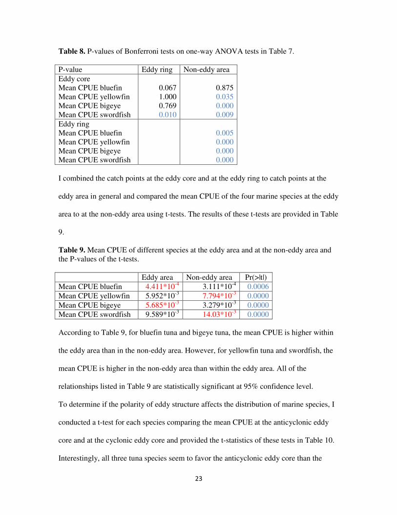
Table 8. P-values of Bonferroni tests on one-way ANOVA tests in Table 7.

P-value Eddy ring Non-eddy area

Eddy core

Mean CPUE bluefin

Mean CPUE yellowfin

Mean CPUE bigeye

Mean CPUE swordfish

0.067

1.000

0.769

0.010

0.875

0.035

0.000

0.009

Eddy ring

Mean CPUE bluefin

Mean CPUE yellowfin

Mean CPUE bigeye

Mean CPUE swordfish

0.005

0.000

0.000

0.000

I combined the catch points at the eddy core and at the eddy ring to catch points at the

eddy area in general and compared the mean CPUE of the four marine species at the eddy

area to at the non-eddy area using t-tests. The results of these t-tests are provided in Table

9.

Table 9. Mean CPUE of different species at the eddy area and at the non-eddy area and

the P-values of the t-tests.

Eddy area Non-eddy area Pr(>|t|)

Mean CPUE bluefin 4.411*10-4

3.111*10-4

0.0006

Mean CPUE yellowfin 5.952*10-3

7.794*10-3

0.0000

Mean CPUE bigeye 5.685*10-3

3.279*10-3

0.0000

Mean CPUE swordfish 9.589*10-3

14.03*10-3

0.0000

According to Table 9, for bluefin tuna and bigeye tuna, the mean CPUE is higher within

the eddy area than in the non-eddy area. However, for yellowfin tuna and swordfish, the

mean CPUE is higher in the non-eddy area than within the eddy area. All of the

relationships listed in Table 9 are statistically significant at 95% confidence level.

To determine if the polarity of eddy structure affects the distribution of marine species, I

conducted a t-test for each species comparing the mean CPUE at the anticyclonic eddy

core and at the cyclonic eddy core and provided the t-statistics of these tests in Table 10.

Interestingly, all three tuna species seem to favor the anticyclonic eddy core than the

24

cyclonic eddy core while the swordfish’s case appears to be the opposite. The difference

in mean CPUE at eddy cores with different polarities is considered statistically significant

at 95% confidence level for all four species.

Table 10. Mean CPUE of different species at eddy cores with different polarities and the

P-values of the t-tests.

Anticyclonic eddy core Cyclonic eddy core Pr(>|t|)


4.970*10-5

0.0152


3.432*10-3

0.0107


3.795*10-3

0.0436


1.655*10-2

0.0004

I conducted similar t-tests to compare the difference in mean CPUE of these four marine

species at eddy rings with different polarities and summarized the results and the P-

values of these t-tests in Table 11.

Table 11. Mean CPUE of different species at eddy rings with different polarities and the

P-values of the t-tests.

Anticyclonic eddy ring Cyclonic eddy ring Pr(>|t|)


2.562*10-4

0.0003


4.727*10-3

0.0942


4.600*10-3

0.0046


18.67*10-3

0.0000

Similar patterns were observed that all the tuna species favor anticyclonic eddy ring over

cyclonic eddy ring while swordfish favors cyclonic eddy ring over anticyclonic eddy ring.

All the differences in mean CPUE between eddy rings with different polarities are

statistically significant at 95% confidence level except for the difference for yellowfin

tuna, which is close to significant. If considering 90% confidence level, it would become

significant.

I then combined the catch points at the anticyclonic eddy core and at the anticyclonic

eddy ring to the catch points at the anticyclonic eddy in general as well as the catch

25

points at the cyclonic eddy core and at the cyclonic eddy ring to the catch points at the

cyclonic eddy in general and compared mean CPUE of the four marine species at eddy

area with different polarities using t-tests and provided the results and the P-values of

these t-tests in Table 12. According to Table 12, all three tuna species favor anticyclonic

eddy over cyclonic eddy while swordfish favors cyclonic eddy over anticyclonic eddy

and all of these relationships are statistically significant at 95% confidence level.

Table 12. Mean CPUE of different species at eddies with different polarities and the P-

values of the t-tests.

Anticyclonic eddy Cyclonic eddy Pr(>|t|)


2.084*10-4

0.0000


4.427*10-3

0.0173


4.413*10-3

0.0007


18.18*10-3

0.0000

In summary, comparing mean CPUE at the eddy area and at the non-eddy area, bluefin

tuna and bigeye tuna favor eddy area over non-eddy area while yellowfin tuna and

swordfish favor non-eddy area over eddy area. Comparing eddy area with different

polarities, all three tuna species favor anticyclonic eddy over cyclonic eddy while

swordfish favors cyclonic eddy over anticyclonic eddy. The marine species distribution

patterns we observed could be potentially explained by looking at the animals’

physiological limitation, cold tolerance for example, as well as their foraging behavior.

The animal’s cold tolerance depends on the size of the animal. Among these four species,

bluefin tuna has the greatest cold tolerance followed by swordfish followed by bigeye

tuna. Yellowfin tuna has the least cold tolerance. Also, bluefin tuna and yellowfin tuna

are shallow feeder while bigeye tuna and swordfish are deep feeder. More literature

review on marine biology is needed to hypothesize a more complete explanation of the

species distribution patterns I observed in this project.

26

Future Research

I could change the combination of the input parameters of the eddy detection workflow.

When the input parameters are changed, the workflow detects different eddy structures. If

the marine species distribution patterns remain the same when I analyze them with

different structures, we can further confirm that the patterns we observed are actually

happening. If the distribution patterns changed, then we need to be very careful in

defining eddies using different combinations of input parameters.

I can also use higher spatial resolution sea level anomaly maps to detect finer scale eddy

structure. Hycom provides 3 time higher spatial resolution sea level anomaly maps than

the Aviso images I worked with in this project. The disadvantage of using Hycom images

is, instead of 14 years, it only provides 2 years of overlap with the fishery catch we

currently have.

I could expand the study area to the southeast coast of the United States and Gulf Maxico.

We have adequate sea level anomaly maps and fishery catch data to support such extent

of studies.

27

Literature Cited

Bakun, A., 2006: Fronts and eddies as key structures in the habitat of marine fish larvae:

opportunity, adaptive response and competitive advantage. Scientia Marina, 70S2,

105-122.

Brandt, S. B., 1981: Effects of a warm-core eddy on fish distributions in the Tasman Sea

off East Australia. Marine Ecology, 6, 19-33.

Chelton, D. B., M. G. Schlax, R. M. Samelson, and R. A. de Szoeke, 2007: Global

observations of large oceanic eddies. Geophysical Research Letters, 34, L15606,

doi:10.1029/2007GL030812.

Gasca, R., 2003a: Hyperiid amphipods (Crustacea: Peracarida) in relation to a cold-core

ring in the Gulf of Mexico. Hydrobiologia, 510, 115-124.

Gasca, R., 2003b: Hyperiid amphipods (Crustacea: Peracarida) and spring mesoscale

features in the Gulf of Mexico. Marine Ecology, 24(4), 303-317.

Henson, S. A. and A. C. Thomas, 2008: A census of oceanic anticyclonic eddies in the

Gulf of Alaska. Deep Sea Research I, 66, 163–176.

Isern-Fontanet, J., E. Garcia-Ladona, and J. Font, 2006: Vortices of the Mediterranean

Sea: An altimetric perspective. Journal of Physical Oceanography, 36, 87-103.

Logerwell, E.A., and P. E. Smith, 2001: Mesoscale eddies and survival of late stage

Pacific sardine (Sardinops sagax) larvae. Fisheries Oceanography, 10, 13-25.

McGillicuddy, D. J., and A. R. Robinson, 1997: Eddy induced nutrientsupply and new

production in the Sargasso Sea. Deep Sea Research I, 44, 1427-1450.

Olson, D., 1991: Rings in the ocean. Annual Review of Earth and Planetary Sciences, 19,

283-311.

28

Paterson, H. L., B. Knott, and A. M. Waite, 2007: Microzooplankton community

structure and grazing on phytoplankton, in an eddy pair in the Indian Ocean off

Western Australia. Deep Sea Research II, 54, 1076-1093.

Richardson, P. L., 1983: Eddy kinetic energy in the North Atlantic Ocean from surface

drifters. Journal of Geophysical Research, 88, 4355-4367.

Roberts, J. J., B. D. Best, D. C. Dunn, E. A. Treml, and P. N. Halpin, in press: Marine

Geospatial Ecology Tools: An integrated framework for ecological

geoprocessing with ArcGIS, Python, R, MATLAB, and C++. Environmental

Modelling & Software.

Wyrtki, K., L. Magaard, and J. Hager, 1976: Eddy energy in the oceans. Journal of

Geophysical Research, 81, 2641-2646.

Documents

North Atlantic Mesoscale Eddy Detection and Marine Species