Embed Size (px)
Citation preview

NORC Methodological Research to Support the Redesign of the
National Crime Victimization Survey
Fall 2009

NORC Methodological Research to Support the Redesign of the National Crime Victimization Survey: Analysis of Possible NonResponse Bias (Competitive ID Number 2008‐BJS‐1834D)
Presented to: U.S. Department of Justice
e Programs tatistics
Office of JusticBureau of Justice S
er Erika Harrell rogram Manag02‐307‐0758 P2
enter (NORC) Presented by:
arch Cicago
National Opinion Resef Cheet
at the University otr1155 East 60th S
Chicago, IL 60603 (773) 256‐6000 (773) 753‐7886 (Fax)
Fall 2009

i. | P a g e
Table of Contents
Chapter 1. Background and Study Scope ..................................................................................... 1
1.1 Background ........................................................................................................................................... 1 1.2 Types of Nonresponse ...................................................................................................................... 2 1.3 Working Hypotheses ......................................................................................................................... 5
........................................................................... 8 1.4 Working Tools ...........................................................Chapter 2. Capture‐Recapture Model of Potential Bias ........................................................... 11
2.1 Introduction ....................................................................................................................................... 11 2.2 NCVS Longitudinal Data and Interview Status across Waves ...................................... 12 2.3 Fraction of Nonresponse That Is Ignorable ......................................................................... 14 2.4 Ignorable Nonresponses and Returning Interviews by Subgroups .......................... 15 2.5 Discussion ........................................................................................................................................... 19
le Cohort .......................... 20 2.6 Imputation and Its Impact on the 2002 NCVS New SampChapter 3. Response Analysis of Early vs. Late and Key Subgroups ....................................... 24
3.1 Introduction ....................................................................................................................................... 24 3.2 Early vs. Late and Easy vs. Hard Responder Comparisons ............................................ 25 3.3 Modeling Continued Response and Characteristics of Drop Outs .............................. 29 3.4 Differential Response Rates and Dispositions by Subgroups ...................................... 31
............................................. 34 3.5 More on Responder Differences ..................................................Chapter 4. R Crime Statistics at the An Analysis of the NCVS and UC
at the County‐Level, 2003‐2006............................................................................... 38
4.1 Introduction ....................................................................................................................................... 38 4.2 Data Sources ...................................................................................................................................... 39 4.3 Measurement ..................................................................................................................................... 40 4.4 Results .................................................................................................................................................. 41 4.5 Outliers ................................................................................................................................................. 43
d UCR ............................................................................. 44 4.6 Relationship between the NCVS anChapter 5. Summary and Recommendations ............................................................................ 47
5.1 Summary ............................................................................................................................................. 47 ecommendations for Immediate Action ............................................................................. 47 5.2 R ................................................................................................................................... 50 Appendix A
Appendix B ................................................................................................................................... 54

i. | P a g e
Appendix C .............................................................................................................................. ................................................................................................................................... 75
..... 61
Appendix D ................................................................................................................................... 90 Appendix E................................................................................................................................... 97 Appendix F
Appendix G ................................................................................................................................. 113
Introduction ...................................................................................................................................................... 113 Ideas for Implementation over the Coming Months ....................................................................... 113 Conclusion ......................................................................................................................................................... 120

1 | P a g e N O R C — A n a l y s i s o f P o s s i b l e N o n ‐ R e s p o n s e B i a s
Chapter 1
Background and Study Scope
This Report is divided into 4 main chapters, plus a summary (Chapter 5) and several
appendices that contain details about the work NORC did on NCVS nonresponse issues.
Included, too, is supporting information that can be used to broaden interpretations by
NVCS experts beyond the conclusions offered here.
We have chosen, for the most part, to footnote technical details and references, as
the report proceeds. But to those who want to approach this material in a nonsequential
fashion we will also provide a glossary separately, on request.
1.1 Background
The measurement of crime and the validity and reliability of crime statistics have
long been of concern to social scientists.1 For much of the twentieth century the Uniform
Crime Reports (UCR) produced by the Federal Bureau of Investigation (FBI) were
considered “almost sacrosanct” as a source of official crime statistics in the United States.2
However, by the late twentieth century there were a large number of studies questioning
the extent to which UCR statistics can be treated as an accurate and adequate measure of
crime.
To address these concerns, in 1973 the Bureau of Justice Statistics (BJS) introduced
the National Crime Victimization Survey (NCVS, formerly NCS), which is fielded by the US
Census Bureau. The purpose of that survey was “to learn more about crimes and the
victims of crime [and] to measure crimes not reported to police as well as those that are
reported.3” Data are collected twice a year from a nationally representative sample to
obtain information about incidents of crime, victimization, and trends involving victims 12
1 For example, see Biderman, A. 1967. “Surveys of Population Samples for Estimating Crime Incidence,”
Anna n Academy of Political an and Biderman, A. 1981. “Sou The Journal
ls of the America d Social Science, 374 (1967): 16‐33; r of Criminal Law and Crimino
logy (New York: McGraw Hill, 196ces of Data for Victimology,” logy, 72 (1981): 789‐817.
2 Savitz, L. 1967. Dilemmas in Crimino 7), 31. 3 Bureau of Justice Statistics, Report to the Nation on Crime and Justice, 2nd ed., NCJ‐105506 (Washington,
DC: US Department of Justice, 1988), 11.
2 | P a g e N O R C — A n a l y s i s o f P o s s i b l e N o n ‐ R e s p o n s e B i a s
years of age and older and their households. The survey has long been considered a leader
in making methodological advances.4 The survey underwent an “intensive methodological
redesign” in 1993 to “improve the questions used to uncover crime, update the survey
methods, and broaden the scope of the crimes measured.5”
The UCR and the NCVS differ in that they “are conducted for different purposes, use
different methods, and focus on somewhat different aspects of crime” (BJS 2004:1). So
inevitably there are discrepancies between estimates derived from these two different
measures of crime. Nonetheless, “long‐term [NCVS and UCR] trends can be brought into
close concordance” by analysts familiar with the programs and data sets.6 This is not
surprising in that the NCVS was designed “to complement the UCR program.7” So while the
NCVS and UCR programs each were designed to collect different data, each offers data that
are criminologically relevant, together they “provide a more complete assessment of crime
in the U 8nited States. ”
The conclusion is that both programs are essential to the measurement of crime in
the United States. So, while we will concentrate mainly on the NCVS, we make a modest
parallel effort involving the UCR and highlight the possible joint use of both of these
statistical series, in a manner that parallels the use by the Bureau of Labor Statistics (BLS)
of employment and unemployment data, from the Current Population Survey and the
Current Employment Program.
1.2 Types of Nonresponse
Operationally, two major components of survey nonresponse are conventionally
considered – nonresponse due to noncontact and nonresponse due to refusal. The
literature demonstrates that both noncontact rates and refusal rates have been on the rise
4 Scheuren, F., What Is a Survey? 2000. www.whatisasurvey.info (accessed Sept 9). ember 30, 2005 reau of Justice Statistics, The Nation’s Two Crime Measures, NCJ‐122705
(Wa artment of Justice, 2004), 1. For example, see Bus ephington, D.C.: US D6 BJS 2004:2. Ibid., 2. 7 BJS 2004:2. Ibid. 8 Lauritsen, J.L. and Schaum, R.J. 2005. “Crime and Victimization in the Three Largest Metropolitan Areas,
198098,” NCJ 208075 (Washington, D.C.: Bureau of Justice Statistics), http://www.ojp.usdoj.gov/bjs/pub/pdf/cv3lma98.pdf (accessed September 30, 2009).

3 | P a g e N O R C — A n a l y s i s o f P o s s i b l e N o n ‐ R e s p o n s e B i a s
in the recent decade and that, in face‐to‐face surveys, refusals can now be a larger
component of nonresponse than noncontacts.9 “Uncorrectable” nonresponse bias may
arise mainly from noncontact nonresponse, since typically in such settings‐‐ like the first
wave of the NCVS‐‐we have very little to go on in adjusting for the nonresponse.10 Refusal
nonresponse, on the other hand, often rises after a first contact, when some information is
known about the respondents. What we know about the nonrespondents allows us to
usefully distinguish among three models, first proposed by Rubin:11
Ignorable nonresponse: If the probability that a household or a within‐household
individual selected for the NCVS sample does not depend on the vector of information
known about the sampling unit (such as geographic region, household income, race,
gender, age, etc.), the response of interest (such as variables about victimization status), or
the survey design, then the nonresponses are ignorable and can be treated as “missing
completely at random” (MCAR). These nonresponses would be essentially selected at
random from the sample and, therefore, can be ignored as a source of bias. They do,
however, increase costs and raise concerns about the credibility of survey estimates.12
Conditional ignorable nonresponse: If the probability that a household or a within‐
household individual selected for the NCVS sample depends on the vector of
information known about the sampling unit but not on the response of interest, the
nonresponse can be treated as missing at random (MAR), given covariates. The
nonresponse can be conditionally ignorable since we may use models to explain the
9 See Atrostic, B. K. et al. 2001. “Nonresponse in U.S. Government Household Surveys: Consistent
Measures, Recent Trends, and New Insights,” Journal of Official Statistics 17: 209‐226. 10 Also, in some surveys like the CPS, a household that was not at home may be an indicator that the
household members could be working. Temporary absent nonresponders in the CPS might, on the other hand, be on vacation.
11 Rubin, D. 1978. “Multiple Imputations in Sample Surveys: A Phenomenological Bayesian Approach to Nonresponse,” Proceedings of the Survey Research Methods Section, American Statistical Association (1978): 20‐28. See also D. Rubin, “Inference and Missing Data,” Biometrika 63, no. 3 (1976): 581‐592.
12 It is important to note that so far we have been talking about the bias of a single univariate variable. We will continue to do so but caution that, as mentioned in Scheuren, F. 2005. “Seven Model Motivated Rules of Thumb or Equations,” http://www.niss.org/sites/default/files/Scheuren.pdf (accessed on September 30, 2009, most of the time all forms of nonresponse are present, sometimes for different variables, sometimes for different time periods.

4 |
P a g e N O R C — A n a l y s i s o f P o s s i b l e N o n ‐ R e s p o n s e B i a s
nonresponse mechanism, and the nonresponse can be ignorable after the model
accounts for it.13
Nonignorable nonresponse: If the probability of nonresponse depends on the value
of a response variable such as victimization status and cannot be completely
explained by the value of the vector of information known about the sampling units
(household or individuals within a household), then the nonresponse is
nonignorable or not missing at random (NMAR). Theoretically, by using additional
covariates, perhaps from an augmented frame or from an earlier wave of the same
survey, models can help in this situation. Make no mistake about the NMAR case,
though; it can seldom be dealt with satisfactorily for the entire vector of survey
variables. There are many cases, however, where, relative to sampling error, the
mean square error (MSE) increase over the sampling variance (VAR) is small, i.e.,
{MSE/VAR}1/2 lies within a narrow range not much larger than if there had been no 14nonresponse, and hence confidence intervals are not unduly lengthened.
In the present Report we distinguish between the concerns about bias that a raw
response rate might engender and measuring the bias arising from nonresponse after
adjusting for it, using whatever is known about the selected units.15 Different survey
approaches may lead to a higher response rate for a similar cost. As pointed out in
13 or study, perhaps from a strong frame or
prev response may be successfully model Obviously the more we know about the unit selected fious successful contacts, the more likely this form of non ed. 14 This point is developed further in Scheuren, F, 2005. “Seven Model Motivated Rules of Thumb or
Equations.” http://www.niss.org/sites/default/files/Scheuren.pdf (accessed on September 30, 2009), in which the following related works are cited: W. G. Cochran, “Sampling Techniques”, 3rd ed. (New York: John Wiley, 1977) ew ; and M. H. Hansen, W. N. Hurwitz, and W. G. Madow, “Sample Survey Methods and Theory”, 2 vols. (NYork: Wiley, 1953).
15 In our treatment here we have largely focused on unit nonresponse concerns, as distinct from item nonresponse. In a complex survey like the NCVS, the line between these two forms of missingness gets blurry. There is a gray area where methods like multiple imputation (Rubin, D. 1978. “Multiple Imputations in Sample Surveys: A Phenomenological Bayesian Approach to Nonresponse,” Proceedings of the Survey Research Methods Section, American Statistical Association (1978): 20‐28) that grew up mainly to handle item nonresponse can be used to handle unit nonresponse just as well or do even better than weighting approaches. For a discussion of this, see the exchange between Little (Little, R. J. A. 1988. “Missing‐Data Adjustment in Large Surveys,” Journal of Business & Economic Statistics 6, no. 3 (1988): 287-296) and Scheuren. Scheuren, F. 1988. “Missing-Data Adjustments in Large Surveys: Comment,” Journal of Business & Economic Statistics 6, no. 3 (1988): 298-299.

5 | P a g e N O R C — A n a l y s i s o f P o s s i b l e N o n ‐ R e s p o n s e B i a s
Scheuren (2005), unit nonrespondents, m, can be divided up into three parts (MCAR, MAR,
nt in any given survey; that is ‐‐ and NMAR), all usually prese
m = mMCAR + mMAR + mNMAR.
For our work with the NCVS, it is important to learn the size of m overall, and,
conditional on that value, how to minimize mNMAR.
The NORC efforts carried out so far have been confined to studies of unit
nonresponse. Based on our prior work16 we have working hypotheses on the relative sizes
of the quantities mMCAR, mMAR, and especially mNMAR. Of course, we do not expect to test all of
our working hypotheses but shall state them for the record in any case.
1.3 Working Hypotheses
The challenges of nonresponse are both very hard and very common. Seldom, like
now, though do we get a chance to explore the nature of unit nonresponse in depth. Still,
because nonresponse is chronic, practitioners (like us) have had a chance to develop
working hypotheses that have proven of value in settings similar to the ones we face with
in the National Crime Victimization Survey (NCVS).
Of course, in our proposal NORC spelled out areas we thought worthy of study.
The wse ere and we paraphrase –
1. A still new modeling approach, labeled “Capture/Recapture,” that uses two or more waves of the NCVS to estimate the average propensity to respond by NCVS wave.17 We cover this in Chapter 2.
2. As an extension of this method, we will divide respondents at one wave between those who continued to remain respondents and those who later became nonrespondents. Particularly important will be differences between the first wave and later wave responders/nonresponders.18 This is covered in Chapter 3.
16 tions” (presentation, International Statistical Institute,
56th Scheuren, F. 2007. “Paradata Inference ApplicaSession, Lisbon, August 22‐29). 17 For example as set out in Scheuren, 2007. Ibid. 18 See also the ideas in Kish and Hess (Kish, L. and Hess, I. 1958. “On Noncoverage of Sample Dwellings,”
Journal of the American Statistical Association 53 (1958): 509‐524), plus the classic Hansen and Hurwitz (Hansen, M. H. and Hurwitz, W. N. 1946. “The Problem of Non‐response in Sample Surveys,” Journal of the

6 | P a g e N O R C — A n a l y s i s o f P o s s i b l e N o n ‐ R e s p o n s e B i a s
3. One standard method involves examining differences between easy and hard‐to‐get NCVS respondents – both households and individuals within selected households – using, say, the 2002‐2006 or other available. We will do this primarily by looking at the survey by wave – also covered in Chapter 3.
4. Another common method we employ is to compare response rates and dispositions among key subgroups. To implement this analysis, we will use the log linear models. Again we will use two or more completed panels of 2002‐2006 NCVS data. See also Chapter 3
5. The final method that NORC proposed compares respondents and nonrespondents directly by using sample frame variables or external data that can be matched to the survey (In particular from the Uniform Crime Reports.19 This is dealt with in Chapter 4.
NORC’s results for each of these areas are detailed in separate later chapters of this
Report. But, first, let us set out our “priors” ‐‐ maybe a better phrase would be our points of
view o, r working hypotheses regarding unit nonresponse:
1. Survey practice regarding nonresponse, including in the NCVS, continues to use methods that grew up in an era of low unit and item nonresponse (the 1940/50s). This is a mistake. These methods need now to be augmented.
2. Organizations, like the US Census Bureau, that pioneered these earlier approaches, notably the application of implicit quasi‐randomization methods20 have stayed with them too long.
3. Costs of attempting to patch these older approaches (e.g., as by refusal conversion) have continued to grow and with no satisfactory way of measurably assessing whether or not they remain effective.
4. There is a very general belief that in a survey setting we need to use more modern methods. But where to start? And how to preserve the many good approaches that still seem to work.
American Statistical Association, 41, no. 236 (1946): 517‐529, republished (in part) in The American Statistician 58, no. 4 (2004): 292‐294.) paper on nonresponse, including the reprint by Scheuren (2004) in the American Statistician. (“with Introduction by Fritz Scheuren on the Topic of Nonresponse or "Missingness").
19 If the frame variables or external data are related both to respondents’ decisions to participate in a survey and to the survey variables of interest, then they are ideal as covariates in that they all researchers to lower rmation on the natu
both the survey variance and bias. This method, thus, yields potentially useful infore of nonresponse and the potential size of nonresponse bias. 20 Oh, H.L. and Scheuren, F. 1983. “Weighting Adjustment for Unit Nonresponse,” in Incomplete Data in
Sample Surveys: Vol. 2, Theory and Bibliographies, eds. W. G. Madow, I. Olkin, and D. B. Rubin (New York: Academic Press).

7 |
P a g e N O R C — A n a l y s i s o f P o s s i b l e N o n ‐ R e s p o n s e B i a s
5. The NCVS has many aspects that offer “handles” to pull existing Census practice up to a more cost effective and inferentially supportive paradigm. We have partially explored some of these, to the extent our scope allowed.
6. The idea of using paradata more in making estimates has been growing but the actual paradata being obtained has not kept pace with the rhetoric. In fact, paradata remains an area that is “underdesigned” for inference.21
7. No surprise, then, that this would be true for the NCVS too! The Census collected paradata in the NCVS were designed to measure or monitor various survey subsystems and we found them very hard to use for addressing broader inference questions.
8. Why? The existing NCVS paradata created by the Census Bureau, have not adhered fully to Deming’s dictum of being designed to “do systems thinking.” In any case,
rall. right now in the NCVS, the Census Bureau is not looking enough at inference ove
9. Perhaps the best example of this failure is that the Census Bureau has really not used the excellent longitudinal structure of the NCVS to improve cross‐section estimates, which seem to be the main focus currently for BJS
10. Another idea that cannot be directly examined for the NCVS is the use of more frame data. The only exception, and this is a big one, is that we have explored augmenting the frame by linking in the Uniform Crime Reports by county. But more on this below (in Chapter 4).
11. Augmenting the NCVS frame might be of special use in reducing the mean square error of the first wave impact of the NCVS nonresponse. This is an especially important problem, given the nonresponse at the first survey wave of the NCVS is quite sizable and may well be nonignorable to an important degree.22
12. We can only speculate that, because of the weak frame variables now being used in the adjustment of first wave nonresponse, a number of other approaches might lead to improvements. Key here is finding a way to add new variables in an affordable way.
13. Which improvements to try requires serious modeling, not simply extending the quasi‐randomization approach to a larger set of covariates, as useful as that might be.
21 The Recent FCSM session (a copy of the papers provided earlier to BJS) bears this out. 22 A special study, not in our scope, would have been required to examine this directly in the NCVS, but
the work of other researchers supports our conjecture (e.g., Sisto, J. and Rendtel, U., “Nonresponse and Attrition Effects on Design‐Based Estimates of Household Income,” in Harmonisation of Panel Surveys and Data Quality: CHINTEX: The Change from Input Harmonisation to Ex‐Post Harmonisation in National Samples of the European Community Household Panel, Implications on Data Quality, M. Ehling et al. (Wiesbaden: Statistisches Bundesamt, 2004).

8 | P a g e N O R C — A n a l y s i s o f P o s s i b l e N o n ‐ R e s p o n s e B i a s
14. NORC cannot offer a modeling approach to nonresponse, without reminding the reader that we are not believers in the notion that a “best model exists and can be found. “
15. Rather, we have become believers in providing multiple estimates (e.g., as with a Bayesian approach) – indeed, in providing a distribution of answers. This approach is still new to Census surveys, although quite common when, say, making demographic (e.g., population) projections (as in the Census P‐20 Series).
16. Much more is to be said about the value of making models explicit, defending them and offering ways for BJS customers, including BJS staffers, to link up their analysis models with the models that data producers, like the Census Bureau, might come up with.23
17. Usually, though, the biggest challenge, especially when a program is operational, is coming up with a way to make changes continuously and affordably.
18. Deming, again, tells us that perhaps the most important quality attribute is “constancy of purpose” or the ability for leaders to stay focused and work for the long run improvements.
19. Deming does not think well of managers, as distinct from leaders. Perhaps he attributes short run thinking to managers, not leaders.
20. Frankly and perhaps too bluntly the NORC recommendations made here are for leaders, not managers. What NORC recommends BJS try are small, affordable yet continuous changes (a Kaisen approach). This would allow them to operate adaptively ‐‐ making a revolution, one small step at a time! In the summary chapter, Chapter 5, NORC highlights some items that we recommend BJS began doing right away.
1.4 Working Tools
The tools NORC recommends are of several types. Some are implied already in our
discussion of working hypotheses above. Some others will allow us to move the focus onto
the implementation process we have in mind. It is very apparent to us and we began with
this observation that the NVCS nonresponse problem is very complex, cannot be separated
from other survey‐ going activities and will require novel use of new tools or old tools used
in new ways. A sampling is given below:
23 For example, see Scheuren, F. 2005. “Seven Model Motivated Rules of Thumb or Equations,”
ttp://www.niss.org/sites/default/files/Scheuren.pdfh (accessed on September 30, 2009).
9 |
P a g e N O R C — A n a l y s i s o f P o s s i b l e N o n ‐ R e s p o n s e B i a s
First, we talked about the need for more use of a redesigned paradata system for the
survey as a whole. This might be of most importance to second and subsequent
waves.
Second, we mentioned an augmented frame for the survey, to the extent affordable.
This might be particularly valuable for first wave nonresponse, where so little else is
known.
Third, any proposed modern “solution” would need explicit use of nonresponse
models and the display of alternative estimates that allow survey analysts to look at
sensitivity issues routinely.
Fourth, we recommend that there be a direct use of earlier survey waves in making
inferences at later waves. Familiar examples here might be the use of multiple
survey weights and, for some variables; multiple imputation might be tried too.
Fifth, a redesigned data collection strategy that cuts way down on the reliance that
now exists in the NCVS on callbacks. Callbacks implicitly assume all nonresponse is
nonignorable when, as our work suggests (See Chapter 2) for the NCVS this may be
far from true.
Sixth, we do not advocate eliminating callbacks but replacing by a focused but
smaller, more intensive field effort to address the interpretation that nonignorable
nonresponse poses.
Seventh, we strongly suggest the collection of more data about interviewers and a
direct use of the interviewer‐to‐interviewer variability for inference. This is
arguably paradata but so important that it deserves special mention.
Eighth, we would also look at the existing reinterview program (a look we were not
commissioned to do). It might be integrated into the main NCVS estimates, partly for
interpretative reasons and partly for improvement reasons.

10 | P a g e N O R C — A n a l y s i s o f P o s s i b l e N o n ‐ R e s p o n s e B i a s
Ninth, we believe the greatest value NORC will offer here is our ability to triangulate
or borrow insights from each method to create an overall view of the nonresponse
surface in the recent rounds of the NCVS.
Tenth, we expect to make recommendations about how to better measure the
biasing portion of nonresponse in the NCVS. With these measures it may be possible
to redirect resources to better target future survey efforts and to better measure
biases and their effect on survey inference. The results will be used to inform better
post‐survey adjustment procedures.
Eleventh, Little and Zhang in the new book edited by Peter Lynn makes four
recommendations which we see as key to a redirected nonresponse program. 24
At the design stage, record values of covariates that are predictive of nonresponse, and condition on these in imputing the missing values
Consider following up a subsample of nonrespondents to recover at least the key missing information on these cases. These data can then be used to multiply‐impute the information on incomplete cases that are not followed up.
When there are various mechanisms of missingness, attempt to determine which of the missing values of a variable are likely to be MAR and which are likely not to be MAR, and then use MAR methods to multiply‐impute the former. This reduces the scope of the NMAR problem for this variable, as compared with an analysis that fits a NMAR model to all the missing values.
In a separate appendix we provide still other improvement suggestions that were
provided earlier but, for the most part, will not be developed here, accept on a limited basis
in the summary Chapter 5
24 Lynn, P. 2009. “Methodology of Longitudinal Surveys,” (New York: Wiley).
11 | P a g e N O R C — A n a l y s i s o f P o s s i b l e N o n ‐ R e s p o n s e B i a s
Chapter 2
CaptureRecapture Model of Potential Bias
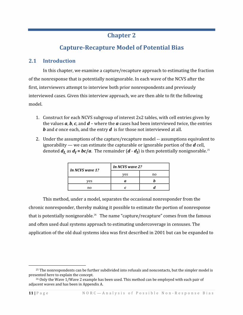
2.1 Introduction
In this chapter, we examine a capture/recapture approach to estimating the fraction
of the nonresponse that is potentially nonignorable. In each wave of the NCVS after the
first, interviewers attempt to interview both prior nonrespondents and previously
interviewed cases. Given this interview approach, we are then able to fit the following
model.
1. Construct for each NCVS subgroup of interest 2x2 tables, with cell entries given by the values a, b, c, and d – where the a cases had been interviewed twice, the entries b and c once each, and the entry d is for those not interviewed at all.
2. Under the assumptions of the capture/recapture model ‐‐ assumptions equivalent to ignorability — we can estimate the capturable or ignorable portion of the d cell, denoted dI, as dI = bc/a. The remainder (d ‐ dI) is then potentially nonignorable.25
In NCVS w 1? aveIn NC ave 2? VS w
yes no yes a b
no c d
This method, under a model, separates the occasional nonresponder from the
chronic nonresponder, thereby making it possible to estimate the portion of nonresponse
that is potentially nonignorable.26 The name “capture/recapture” comes from the famous
and often used dual systems approach to estimating undercoverage in censuses. The
application of the old dual systems idea was first described in 2001 but can be expanded to
25 el is The nonrespondents can be further subdivided into refusals and noncontacts, but the simpler mod
presented here to explain the concept. 26 Only the Wave 1/Wave 2 example has been used. This method can be employed with each pair of
adjacent waves and has been in Appendix A.

cover a survey, like the NCVS, that has 7 waves.27 Now, of course, there may be dependency
across waves that would need to be modeled before the results were used. We do not
believe, based on earlier applications28 that this will be an insurmountable barrier, if
handled properly.
What we are doing is treating those households29 that respond on some occasion(s)
but not others as missing at random (MCAR or MAR), while the “never responders” are
more likely to be nonignorable (NMAR). The base and follow‐up interviews for NCVS can,
thus, be used under this model to estimate the portion of nonresponse that is potentially
nonignorable. 30 Typically, in longitudinal surveys, and the NCVS would seem to be no
different, attrition or chronic nonresponse becomes more and more common in later
waves. In some longitudinal surveys, once a refusal occurred in an earlier wave, no further
attempts were made in later waves. This is not the case with the NCVS, and we have used
that fact in a manner similar to that used in Vaughan and Scheuren.31
2.2 NCVS Longitudinal Data and Interview Status across Waves
Each month the U.S. Census Bureau selects respondents for the NCVS using a
“rotating panel” sample design. Households are randomly selected and all age‐eligible
individuals become part of the panel. Once in the sample, respondents are interviewed
P a g e N O R C — A n a l y s i s o n ‐ R e s p o n s e B i a s o f P o s s i b l e N
27 Scheuren, F. 2001. “Macro and Micro Paradata for Survey Assessment,” in 1999 NSAF Collection of
Papers, by Tamara Black et al. and J. Michael Brick et al., 2C‐1 – 2C‐15 Washington, D.C.: Urban Institute, ethodology_7.pdfhttp://anfdata.urban.org/nsaf/methodology_rpts/1999_M . See also
http://www.unece.org/stats/documents/2000/11/metis/crp.10.e.pdf (both accessed on October 2, 2009). Assessing the New Federalism Methodology Report No. 7.
28 Scheuren, F. 2007. “Paradata Inference Applications,” presented at the 56th Session of the InternationalStatistical Institute, Lisbon, August 22‐29.
29 We do not know enough about the use of this model for the sampling of individuals within households, so we have not offered it for use here. A future study of this would be recommended, if enough resources were available. There are other priorities that would be placed higher, however. See Chapter 6.
30 The fact that a household never responds does not mean that it is biasing and nonignorable. It could have characteristics very similar to those of respondents; hence we have characterized this group as only poten n a rate which treats all of the n
12 |
tially nonignorable. Still, it is better that we use this unit nonresponse rate thaonrespondents as potentially nonignorable. 31 Vaughan, D. and Scheuren, F. 2002. “Longitudinal Attrition in SIPP and SPD,” Proceedings of the Survey
Research Methods Section, American Statistical Association (2002): 3559‐3564.

13 |
P a g e N O R C — A n a l y s i s o f P o s s i b l e N o n ‐ R e s p o n s e B i a s
every six months for a total of seven interviews over a three‐year period.32 For example, we
constructed a longitudinal file for the households that came into the NCVS sample as the
new incoming units to be interviewed for the first time in 2003. Two cohorts of NCVS
households were setup, with first cohort containing households starting to be approached
for interviews for the first time within the first six months of 2003, and the second cohort
containing households starting to be interviewed for the first time within the second six
months of 2003. Each of the households in these two cohorts can stay in the sample to be
interviewed seven times for seven waves, till the first half of 2006 and the second half of
2006 respectively.
Noninterviews may occur at any of the waves for any of the households approached
for interviews. A sample unit for which an interview could not be obtained is classified as
one of 33three non‐interview types, namely, Type A, Type B, and Type C noninterviews .
Tables 2.1 and 2.2 summarize the statuses of the households in the two cohorts
across the seven waves starting from 2003. Take table 1 for example, among the 9,363
“incoming” households in the first cohort of 2003; there were 6,898 interviewed in the first
wave, 1,372 were Type B non‐interviews, 416 were Type C non‐interviews, and the rest
were Type A non‐interviews (336 refusals, 236 with no one at home, and 105 for other
Type A reasons). In each of the subsequent waves, some households were not linked for
reasons such as their moving out of the sample. These, so called “not matched” cases were
excluded from this analysis and excluded in the paired 2x2 capture/recapture analysis.
32National Crime Victimization Survey, 2007 [RecordType Files]: Codebook (Ann Arbor, MI: Inter‐
university Consortium for Political and Social Research, 2009), http://www.icpsr.umich.edu/cgi‐bin/bob/archive2?study=25141&path=NACJD&docsonly=yes (accessed on October 5, 2009).
33 Type A non‐interviews consist of households occupied by persons eligible for interviews but from whom non interviews were obtained because, for example, no one was found at home in spite of repeated visits, the household refused to give any information, the unit cannot be reached due to Type B non‐interviews are for units which are unoccupied or which are occupied solely by persons who have a usual residence elsewhere (URE). Type C cases are ineligible addresses arising because of impassable roads, serious illness or death in the family, or the interviewer is unable to locate the sample unit. Because Type A non‐interviews are considered avoidable, every effort is made to convert them to interviews. The “every effort” is extremely conservative and expensive strategy, especially given that much of the missingness may be ignorable.

14 |
P a g e N O R C — A n a l y s i s o f P o s s i b l e N o n ‐ R e s p o n s e B i a s
Table 2.1: Summary of Interview Status of Households Starting in the First SixMonths of 2003
Wave Not
Matched Interviewed Type A
Type B T Cy pe
R edefus No O omene H O r the Total 1 . 6,898 336 236 105 1,372 4 16 9,3632 641 6,806 330 205 104 1,230 47 9,3633 667 6,789 363 181 91 1,245 27 9,3634 703 6,783 383 164 87 1,224 1 9 9,3635 1,276 6,226 423 169 87 1 ,169 1 3 9,3636 1,662 5,903 385 155 65 1 ,185 8 9,3637 4,266 4,043 250 117 37 643 7 9,363
Note: The period from Wave 1 to Wave 7 spans from 2003Q1Q2 to 2006 Q1Q2. Source: NCVS 2003‐2006
Table 2.2: Summary of Interview Status of Households Starting in the Second SixMonths of 2003
Wave Not
Matched Interviewed Type A
T ype B T y Cpe Total Re d fuse No O ome ne H Other 1 . 6,924 339 275 108 1,383 4 68 9,4972 740 6,881 306 183 92 1,250 45 9,4973 803 6,748 352 192 86 1,287 29 9,4974 1,306 6,307 370 216 73 1 ,201 24 9,4975 1,694 5,964 359 1 74 84 1 ,199 23 9,4976 4,485 3,861 290 1 21 35 692 13 9,4977 4,446 3,964 232 82 55 698 20 9,497
N
ote: The period from Wave 1 to Wave 7 spans from 2003Q3Q4 to 2006 Q3Q4.
2.3 Fraction of Nonresponse That Is Ignorable
A key promising feature of the capture‐recapture method for NCVS nonresponse
analysis is its capacity to estimate the fraction of nonresponse that is ignorable and how
the fractions of ignorable nonresponse can vary for various subgroups. To test the fraction
of nonresponse that is ignorable, we examined the interview statuses for the whole range
of the pairs of 2x2 waves, with the current wave tabulated by each of all the subsequent
waves.
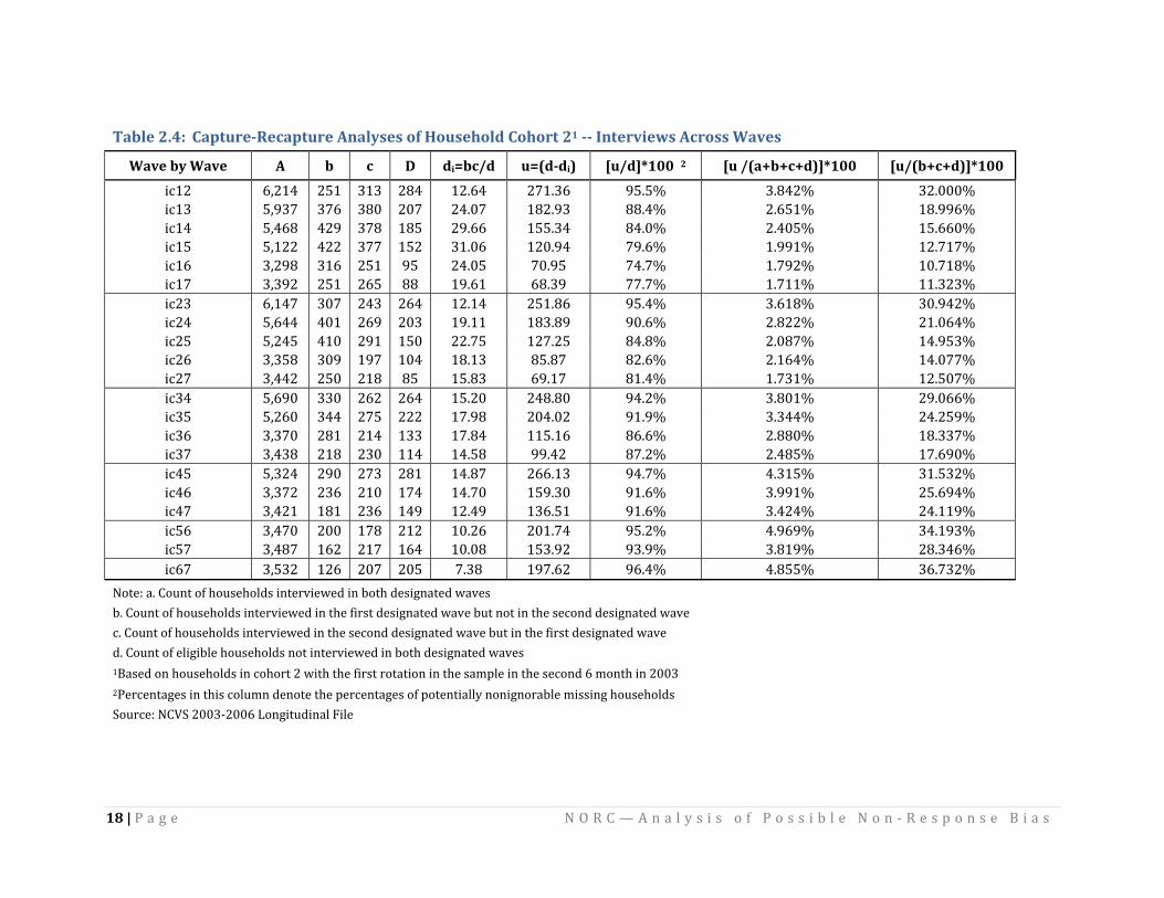
Table 2.3 and Table 2.4 show the capture‐recapture analysis results on the
interview status across waves among cohort 1 and cohort 2 households respectively. The
last columns under [u/(b+c+d)]*100 calculate the fractions of nonresponses that may not

15 |
P a g e N O R C — A n a l y s i s o f P o s s i b l e N o n ‐ R e s p o n s e B i a s
be ignorable. For any of the 2x2 pair of the waves, the fraction of nonresponse that is not
ignorable falls into the range between about 10% to slightly less than 40%. That is, the
majority of the nonresponses can be treated as ignorable. The results also reveal that the
farther apart the two waves were the proportion of nonignorable nonresponses would be
smaller.
The capture/recapture approach separates nonresponse cases into two forms of
missingness ‐‐ ignorable and potentially nonignorable. This is, of course, under an
independence model. The ignorable portion, by definition, is not biasing but does increase
the sampling error because the number of respondents is reduced. It also raises the
average cost per usable respondent too. The balance of the missingness is only potentially
nonignorable. The balance, too, could be ignorable, if a more refined model were used. The
interpretation of the capture/recapture results is based on the notion that some
nonresponse is chronic, coming from units that never respond and some nonresponse is or
behaves as if it were “random,” coming from units that would respond or even do respond
another time. In our treatment here we are using the model results as a lower bound on
the ignorable nonresponse.
2.4 Ignorable Nonresponses and Returning Interviews by Subgroups
As an extension of the capture/recapture method, we divide respondents at one
wave between those who continued to remain respondents and those who later became
nonrespondents. The panel data of NCVS have considerable information about
nonrespondents who participated in some earlier wave. There are data available on
demographic and victimization characteristics; therefore, it is possible to discern
differences between these individuals and those who continued to respond. In addition,
study of later wave nonrespondents helps not only to develop nonresponse weighting
adjustments34 but also to gain an understanding of the causes of panel attrition35 Tables
34 Oh, L. and Scheuren, F. 1983. “Weighting Adjustment for Unit Nonresponse,” in Incomplete Data in
Sampl ol. 2 ork: Acad
e Surveys: V , Theory and Bibliographies, eds. W. G. Madow, I. Olkin, and D. B. Rubin (New Yemic Press. 1983). 35 Kalton, G. et al.. 1992. “Characteristics of Second Wave Nonrespondents in a Panel Survey,” Proceedings
of the Survey Research Methods Section, American Statistical Association: 462‐467.
16 | P a g e N O R C — A n a l y s i s o f P o s s i b l e N o n ‐ R e s p o n s e B i a s
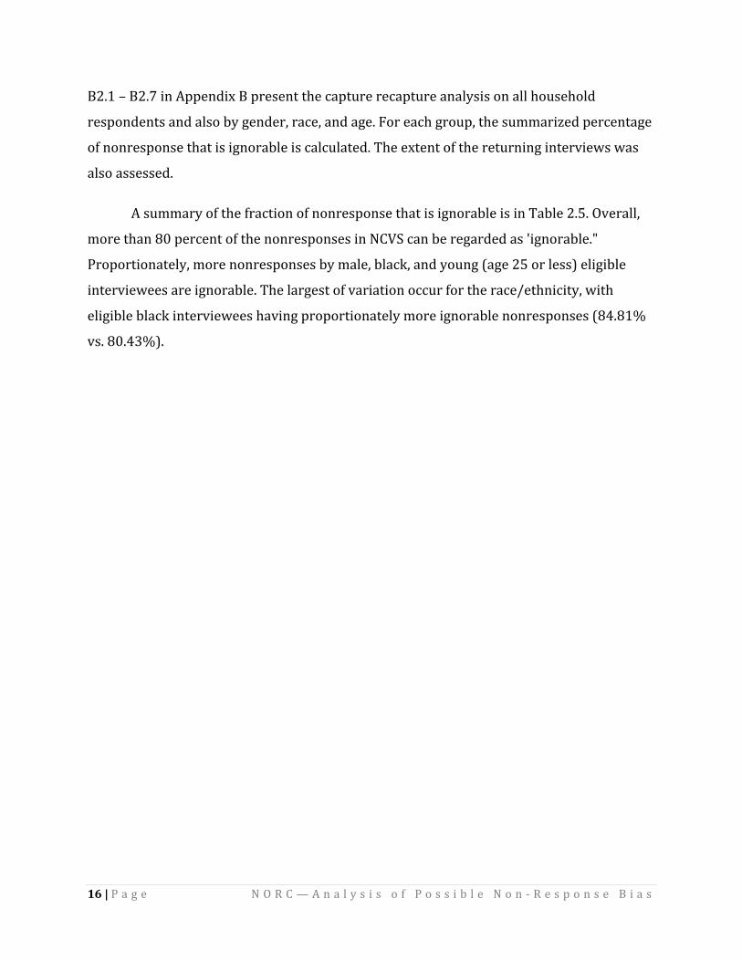
B2.1 – B2.7 in Appendix B present the capture recapture analysis on all household
respondents and also by gender, race, and age. For each group, the summarized percentage
of nonresponse that is ignorable is calculated. The extent of the returning interviews was
also assessed.
A summary of the fraction of nonresponse that is ignorable is in Table 2.5. Overall,
more than 80 percent of the nonresponses in NCVS can be regarded as 'ignorable."
Proportionately, more nonresponses by male, black, and young (age 25 or less) eligible
interviewees are ignorable. The largest of variation occur for the race/ethnicity, with
eligible black interviewees having proportionately more ignorable nonresponses (84.81%
vs. 80.43%).

Table 2.3 CaptureRecapture Analyses of Household Cohort 11 Interviews Across Waves
Wave Wave by A b c D di a=bc/ u )=(ddi [u 2 /d]*100 [u /(a+b+c+d)]*100 [u/(b+c+d)]*100 ic12 6,156 304 294 275 14.52 260.48 94.7% 3.706% 29.838% ic13 6,013 355 344 218 20.31 197.69 90.7% 2.853% 21.558% ic14 5,912 404 384 178 26.24 151.76 85.3% 2.206% 15.710% ic15 5,419 452 350 163 29.19 133.81 82.1% 2.096% 13.866% ic16 5,086 411 354 143 28.61 114.39 80.0% 1.908% 12.598% ic17 3,473 288 264 80 21.89 58.11 72.6% 1.416% 9.194% ic23 6,134 289 291 279 13.71 265.29 95.1% 3.794% 30.884% ic24 6,008 358 321 236 19.13 216.87 91.9% 3.133% 23.702% ic25 5,457 420 304 201 23.40 177.60 88.4% 2.783% 19.200% ic26 5,111 390 332 169 25.33 143.67 85.0% 2.394% 16.124% ic27 3,491 256 242 109 17.75 91.25 83.7% 2.227% 15.034% ic34 6,142 288 268 291 12.57 278.43 95.7% 3.984% 32.873% ic35 5,559 382 272 237 18.69 218.31 92.1% 3.385% 24.502% ic36 5,183 354 294 192 20.08 171.92 89.5% 2.854% 20.467% ic37 3,548 238 216 130 14.49 115.51 88.9% 2.796% 19.779% ic45 5,685 329 214 298 12.38 285.62 95.8% 4.377% 33.961% ic46 5,276 313 240 246 14.24 231.76 94.2% 3.815% 29.007% ic47 3,589 217 186 150 11.25 138.75 92.5% 3.350% 25.091% ic56 5,250 251 275 297 13.15 283.85 95.6% 4.674% 34.490% ic57 3,571 187 218 176 11.42 164.58 93.5% 3.964% 28.328% ic67 3,646 156 163 206 6.97 199.03 96.6% 4.772% 37.910%
Note: a. Count of households interviewed in both designated waves b. Count of households interviewed in the first designated wave but not in the second designated wave c. Count of households interviewed in the second designated wave but in the first designated wave d. Count of eligible households not interviewed in both designated waves 1Based on households in cohort 1 with the first rotation in the sample in the first 6 month in 2003 2Percentages in this column denote the percentages of potentially nonignorable missing households Source: NCVS 2003‐2006 Longitudinal File
17 | P a g e N O R C — A n a l y s i s o f P o s s i b l e N o n ‐ R e s p o n s e B i a s
18 | P a g e N O R C — A n a l y s i s o f P o s s i b l e N o n ‐ R e s p o n s e B i a s
Table 2.4: CaptureRecapture Analyses of Household Cohort 21 Interviews Across Waves
Wave Wave by A b c D d i=bc/d u =(ddi) [u/d]*100 2 [u /(a+b+c+d)]*100 [u/( 100 b+c+d)]*
ic12 6,214 251 313 284 12.64 271.36 95.5% 3.842% 32.000% ic13 5,937 376 380 207 24.07 182.93 88.4% 2.651% 18.996% ic14 5,468 429 378 185 29.66 155.34 84.0% 2.405% 15.660% ic15 5,122 422 377 152 31.06 120.94 79.6% 1.991% 12.717% ic16 3,298 316 251 95 24.05 70.95 74.7% 1.792% 10.718% ic17 3,392 251 265 88 19.61 68.39 77.7% 1.711% 11.323% ic23 6,147 307 243 264 12.14 251.86 95.4% 3.618% 30.942% ic24 5,644 401 269 203 19.11 183.89 90.6% 2.822% 21.064% ic25 5,245 410 291 150 22.75 127.25 84.8% 2.087% 14.953% ic26 3,358 309 197 104 18.13 85.87 82.6% 2.164% 14.077% ic27 3,442 250 218 85 15.83 69.17 81.4% 1.731% 12.507% ic34 5,690 330 262 264 15.20 248.80 94.2% 3.801% 29.066% ic35 5,260 344 275 222 17.98 204.02 91.9% 3.344% 24.259% ic36 3,370 281 214 133 17.84 115.16 86.6% 2.880% 18.337% ic37 3,438 218 230 114 14.58 99.42 87.2% 2.485% 17.690% ic45 5,324 290 273 281 14.87 266.13 94.7% 4.315% 31.532% ic46 3,372 236 210 174 14.70 159.30 91.6% 3.991% 25.694% ic47 3,421 181 236 149 12.49 136.51 91.6% 3.424% 24.119% ic56 3,470 200 178 212 10.26 201.74 95.2% 4.969% 34.193% ic57 3,487 162 217 164 10.08 153.92 93.9% 3.819% 28.346% ic67 3,532 126 207 205 7.38 197.62 96.4% 4.855% 36.732%
Note: a. Count of households interviewed in both designated waves b. Count of households interviewed in the first designated wave but not in the second designated wave c. Count of households interviewed in the second designated wave but in the first designated wave d. Count of eligible households not interviewed in both designated waves 1Based on households in cohort 2 with the first rotation in the sample in the second 6 month in 2003 2Percentages in this column denote the percentages of potentially nonignorable missing households Source: NCVS 2003‐2006 Longitudinal File

Table 2.5 Ignorable Nonresponses by Subgroups
Percent of Nonresponses
that ar rable e IgnoTotal Counts of Ignorable
Nonresponses All 81.10 2762 Male 84.04 1327 Female 83.43 1 435Black 84.81 469 Other 80.43 2 294Age 25 or Younger 84.11 323 Age 26 or Older 83.74 2441
2.5 Discussion
The longitudinal approach has been regarded as essential to study the performance
of the justice system as a whole and it has been recommended that strategies for improving
longitudinal structures, including improving the linkage capacity of existing data to fielding
panel surveys of crime victims.36 NORC heartily concurs, as we found at many points in our
analyse s where some research objectives had to be accomplished only indirectly, if at all.
The capture‐recapture method proposed for NCVS has implications for the survey
sponsor in that it can test whether there is evidence for a potentially serious nonresponse
bias arising from the unobserved fraction of the refusals. It also has implications for the
expensive refusal conversion process and the extent to which that process should be
pursued based on its seemingly small bias reduction potential. Finally, the raw weighted
nonresponse rate measure in NCVS could be recalibrated to reflect only the potentially
nonignorable portion of the nonresponse. Like most surveys, the raw NCVS nonresponse
rate continues to be used as a quality and credibility measure when, in fact, matters are far
more nuanced. This one simple change could allow BJS to focus resources elsewhere, for
example at the fall‐off in reported crime incidences as the survey proceeds, wave by wave.
P a g o f P o s s i b l e N o n ‐ R e s p o n s e B i a s e N O R C — A n a l y s i s19 |
36 Groves, R.M. and Cork, D.L. 2009. “Ensuring the Quality, Credibility, and Relevance of U.S. Justice
Statistics.” Washington, D.C.: National Academies Press.

20 |
P a g e N O R C — A n a l y s i s o f P o s s i b l e N o n ‐ R e s p o n s e B i a s
2.6 rt Imputation and Its Impact on the 2002 NCVS New Sample Coho
In a separate analysis, we constructed a longitudinal file using the “incoming”
household cohort starting in the first half of 2002 and assess the impact of imputations of
the nonresponses. During the first 6 months of 2002, a total of 9,484 households were
selected in the NCVS sample. As part of the NORC’s study on the possible nonresponse bias,
we keep track of the changes of the interview status each time when the same households
were in the subsequent surveys in the next three years, through the constructions of the
longitudinal file which was based on the 2002‐2005 NCVS. Table 2.6 shows the detailed
survey response status by the waves.
Table 2.6: Tracking the Interview Status of the Same Sampled Household Respondents from 20022005
SurveyS Response tatus
Wave 1 Wave 2 Wa e 3 v Wave 4 Wave 5 Wave 6 Wave 7
Type A Interviewed 7004 6 827 6 745 6 671 6 658 6597 6 131 Refused 348 290 329 381 388 397 365 No One at Home 232 1 63 1 56 1 60 1 56 1 85 1 53 Other Type A 114 96 84 94 88 83 58 Type A Subtotal 7698 7376 7314 7306 7290 7262 6707
Refusal Rate* 4 .52% 3.93% 4.50% 5.21% 5.32% 5 .47% 5.44%
Type B 1298 1223 1249 1251 1252 1246 1176 Type C 488 32 27 22 21 28 18 Total 9484 8 631 8 590 8 579 8 563 8536 7901 Not Matched NA 853 894 905 921 948 1583 NS
ote: Refusal rate = Refuseource: NCVS 2002‐2005
d/Type A Subtotal. NA: Not applicable.
Indeed, some households were interviewed at an early wave but turned out to be a
type A nonresponse case in the subsequent wave. Table 2.7 shows the survey response
status for each of the waves after the initial wave, among those interviewed households in
the immediate previous wave.

21 |
P a g e N O R C — A n a l y s i s o f P o s s i b l e N o n ‐ R e s p o n s e B i a s
Table 2.7: Interview Status for Wave t by Interview Status for Wave (t+1) in a 2002 Household Cohort
Interviewed at W e t av
Interview Status at Wave (t+1)
Interviewed Re d fuse No one at H e om
Other Ty A pe
T ype B Ty C pe Total
t=1 6181 107 78 58 316 1 0 6750 t=2 6187 118 89 67 304 3 6768 t=3 6045 158 97 69 323 4 6696 t=4 6062 124 92 67 287 2 6634 t=5 6031 113 1 16 56 289 5 6610 t=6 5606 96 96 45 261 4 6108
Source: NCVS 2002‐2005
As shown, in Table 2.7, there were a total of (107+78+58) households interviewed
in wave 1, which were Type A nonrespondents later on. These households in various waves
were highlighted with bold in the appendix tables. If, as the capture/recapture model
suggests, most of the wave missingness in the NCVS is ignorable, then elaborate strategies
to address/reduce bias seem overkill and less expensive methods might be tried.
We do not have the scope in this exploratory study to do more than illustrate a
simple way to impute nonresponse at later waves by using response achieved at earlier
waves. In particular, one strategy is to have the values of survey variables of interests be
imputed with the values of the same variables from the previous waves.
Table 2.8 shows the imputation rates for wave 2 to wave 7 household respondents.
The crime incidence by the household respondents is listed, both before and after the
imputations took place. Notice how similar the results are, suggesting that an imputation
strategy, with its smaller variance, would be competitive with the current reweighting
strategy. We are just touching on this rather large subject as a way of emphasizing the
advise that is found in the work of Rod Little, mentioned in Chapter 1.

22 |
P a g e N O R C — A n a l y s i s o f P o s s i b l e N o n ‐ R e s p o n s e B i a s
Table 2.8: Characteristics of HouseholdLevel Crime Incidents Before and After the Imputations
W aveI mputation
Rate1 Incident Rate2
Befo ion re Imputat Afte on r Imputati
t=1 No d ne Use 0.1626214 0.1626214 t=2 5.96% 0.1306577 0.1333805 t=3 6.19% 0.1214233 0.1214718 t=4 6.20% 0.1178234 0.1177086 t=5 5.25% 0.1136978 0.1135273 t=6 3.31% 0.1041382 0.1054699 t= 1.64% 0.1050400 0.1050400 7
Note: 1 “imputation rateIncident #” refers to the tource: NCVS 2002‐2005.
” is calculated as (refused + no one at home + other type A). 2 otal crime incident reports filled by the household respondent. “
S
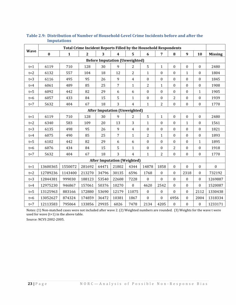
The detailed wave‐specific distributions of the number of crime incidents reported
by household respondents were listed in Table 2.9. Weighted estimations after the
imputations were also listed.
23 | P a g e N O R C — A n a l y s i s o f P o s s i b l e N o n ‐ R e s p o n s e B i a s
Table 2.9: Distribution of Number of HouseholdLevel Crime Incidents before and after the
Imputations
Wave Total Crime Incident Reports Filled by the Household Respondents
0 1 2 3 4 5 6 7 8 9 10 Missing
Before Im tation (Unwe ted) pu igh
t=1 6119 710 128 30 9 2 5 1 0 0 0 2480 t=2 6132 557 1 04 18 1 2 2 1 0 0 1 0 1804 t=3 6116 495 95 26 9 4 0 0 0 0 0 1845 t=4 6061 489 85 25 7 1 2 1 0 0 0 1908 t=5 6092 442 82 29 6 6 0 0 0 0 1 1905 t=6 6057 433 84 15 5 1 0 0 2 0 0 1939 t=7 5632 404 67 18 3 4 1 2 0 0 0 1770
After Imputation Unweighted) ( t=1 6119 710 128 30 9 2 5 1 0 0 0 2480 t=2 6340 583 1 09 20 1 3 3 1 0 0 1 0 1561 t=3 6135 498 95 26 9 4 0 0 0 0 0 1821 t=4 6075 490 85 25 7 1 2 1 0 0 0 1893 t=5 6102 442 82 29 6 6 0 0 0 0 1 1895 t=6 6076 434 84 15 5 1 0 0 2 0 0 1918 t=7 5632 404 67 18 3 4 1 2 0 0 0 1770
After ta ei ) Impu tion (W ghted t=1 13600365 1550072 281692 64471 21802 4344 14878 1858 0 0 0 0 t=2 12789236 1 143400 213270 34796 30135 6596 1768 0 0 2318 0 732192 t=3 12844381 999030 188123 53540 22608 7228 0 0 0 0 0 1269887t=4 12975230 946867 157061 50376 10270 0 4620 2542 0 0 0 1520087t=5 13125963 883166 172880 53690 12179 11075 0 0 0 0 2112 1330438t=6 13052627 874324 174859 36472 10381 1867 0 0 6956 0 2004 1318334t=7 12113583 795064 133856 29935 6026 7478 2134 4205 0 0 0 1233171Notes: (1) Non‐matched caused for wave (t+1) in the Source: NCVS 2002‐2005.
ses were not included after wave 2. (2) Weighted numbers are rounded. (3) Weights for the wave t were above table.

Chapter 3
Response Analysis of Early vs. Late and Key Subgroups
3.1 Introduction
In the proposal, the second intended method to examine bias due to nonresponse
would use a level‐of‐effort approach by contrasting respondents with different levels of
recruitment effort. NORC has applied this approach in nonresponse bias analysis37 and has
found it effective in estimating the direction and the size of nonresponse bias. For the
NCVS, we had proposed to compare survey data for 1) respondents who required less than
three contact attempts/visits vs. respondents who required three or more visits to
complete the survey, and 2) respondents who answered the survey request readily without
refusal conversion effort vs. respondents who required refusal conversion effort.
Unfortunately, the number of attempts to obtain an interview is not a data field readily
available for use – nor is the amount of effort required to convert an initial refusal. These
data may be available on a raw audit file kept by Census on a sample of the interviews.
NORC did ultimately receive a copy of a Raw Audit File, but the amount of effort to decipher
the variables and their meanings did not fit in with the requirements for this study. Thus,
as a proxy, we use differences in estimates between respondents who were amenable and
did not refuse the survey request and those who refused the survey request at least once
but were converted in a later wave.
Several years of data are used to examine stability and trends of the patterns, the
specific data used are shown in Appendix Table C.3.1. Overall, the household and person
level public use files for 2002‐2006, and 2007, as well as the linked household internally
created file for 2002‐2006 are used. Due to the longitudinal nature of the data collection,
previous responses can be used in the same way as frame data to make nonresponse or
missing data adjustments.
P a g e N O R C — A n a l y s i s o f P o s s i b l e N o n ‐ R e s p o n s e B i a s 24 |
37 See Skalland, B. et al. 2006. “A Non‐Response Bias Analysis to Inform the Use of Incentives in Multistage
RDD Telephone Surveys,” Proceedings of the Survey Research Methods Section, American Statistical Association: 3705‐3712.

25 |
P a g e N O R C — A n a l y s i s o f P o s s i b l e N o n ‐ R e s p o n s e B i a s
Throughout this Chapter, results of logistic regression models are presented. We
make no claim that the model results are any “best” predictors of nonresponse; instead, the
purpose of the logistic models is threefold: (1) determining pockets or particular
interactions of characteristics that correlate with response, (2) investigating the
correlation of crime victimization estimates and response patterns, (3) comparing
response patterns across longitudinal data versus annual collection efforts to build on the
natural structure of the data.
3.2 Early vs. Late and Easy vs. Hard Responder Comparisons
The Census Bureau employs a rotating panel longitudinal sample to use for the
NCVS interviews. Each selected household is included in the sample seven times over a
period of three and a half years. Until 2006, the first interview was used as a bounding
interview and not released on the public use file. Beginning in 2006, the first ‘unbounded’
interviews were phased in and included for release. NORC was given access to the internal
files, and created two household level longitudinal cohort files for years 2002‐2006 ‐‐
including the first or unbounded interview. Employing these data, we look at the frequency
of response, by analyzing the distribution of wave response by key demographic variables.
In particular, our exploratory analysis focuses on the panel survey response issue of
continued response and dropout issues – that is, that initial respondents do not continue to
respond through all waves of the survey. There are two issues to address – (1) which
initial respondents are most likely to drop out and (2) after all data are collected, what is
the best way to adjust for the non‐response. The exploratory analysis focuses on singling
out characteristics of drop outs. Using the cohort file NORC created, we looked at initial
responding households that entered the survey in the second half of 2002 and computed
how many waves they participated in.
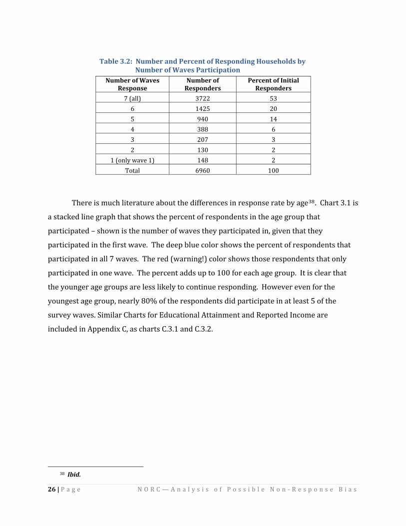
Table 3.2: Number and Percent of Responding Households by
Number of Waves Participation Numb aveser of W
Re e sponsNu ofmber Responders
Percent of Initial Responders
7 (all) 3722 53 6 1425 20 5 940 1 44 388 6 3 207 3 2 130 2
1 (only wave 1) 148 2 Total 6960 100
There is much literature about the differences in response rate by age38. Chart 3.1 is
a stacked line graph that shows the percent of respondents in the age group that
participated – shown is the number of waves they participated in, given that they
participated in the first wave. The deep blue color shows the percent of respondents that
participated in all 7 waves. The red (warning!) color shows those respondents that only
participated in one wave. The percent adds up to 100 for each age group. It is clear that
the younger age groups are less likely to continue responding. However even for the
youngest age group, nearly 80% of the respondents did participate in at least 5 of the
survey waves. Similar Charts for Educational Attainment and Reported Income are
ncluded in Appendix C, as charts C.3.1 and C.3.2. i
P g e N O R C — A n a l y s i s o f P o s s i b l e N o n ‐ R e s p o n s e B i a s a
26 |
38 Ibid.

27 |
P a g e N O R C — A n a l y s i s o f P o s s i b l e N o n ‐ R e s p o n s e B i a s
Chart 3.1: Percent of Responding Households in Age Group
by Number of Waves Participation, Internal Cohort File 20022006
Chart 3.2 below, contains the stacked chart for different categories of household structure.
Response appears higher for households with couples, versus households without couples.

Chart 3.2: Percent of Responding Households by Household Structure
by Number of Waves Participation, Internal Cohort File 20022006
In order to also investigate at the individual response level, Public Use Files (PUF) at
the individual level were downloaded from the ICPSR site managed by University of
Michigan.39 These person level files were merged together in order to look at person level
cohorts beginning in the first half of 2002. Since the first bounding interview is not
included in the Public Use Files, the analysis here focuses on the results from Waves 2
through 7 for both the person level and household cohorts. By focusing on the
panel/rotation group that was initially interviewed in the first half of 2002 (panel/rotation
in 13,23,33,43,53,63), we are able to include all possible responses from that group for the
remaining waves. The patterns are similar for the households and individual
characteristics we examined. Chart 3.3 below is a double chart that compares household
and person level stacked number of waves responded to. Similar charts for Education
Attained, Hispanic Origin, and Race are included in Appendix C, Tables C.3.3 – C.3.5.
28 | P a g e N O R C — A n a l y s i s o f P o s s i b l e N o n ‐ R e s p o n s e B i a s
39 NCVS public use data and documentation are available at http://www.icpsr.umich.edu/NACJD/NCVS/
(accessed on June ‐ September, 2009).

29 |
P a g e N O R C — A n a l y s i s o f P o s s i b l e N o n ‐ R e s p o n s e B i a s
Chart 3.3: Percent of Responding Households and Individuals in Age Group
by Number of Waves Participation, for PUF 20022006
3.3 Modeling Continued Response and Characteristics of Drop Outs
The descriptive charts are informative re overall trends, but we also developed
logistic regression models to explore interactions between the variables. For this exercise,
we use the household cohort files, representing the cohorts beginning in the second half of
2002. As in the household graphs above, we only use records that responded to the first,
bounding wave, and include their continued response. For prediction variables, indicators
and grouped variables were developed for the following variables of interest. Also,
interactions for race and Hispanic origin with the other variable groups were introduced.40
40 Since not all units responded to the first wave, the value used for the independent variable was taken from
the earliest wave response available.
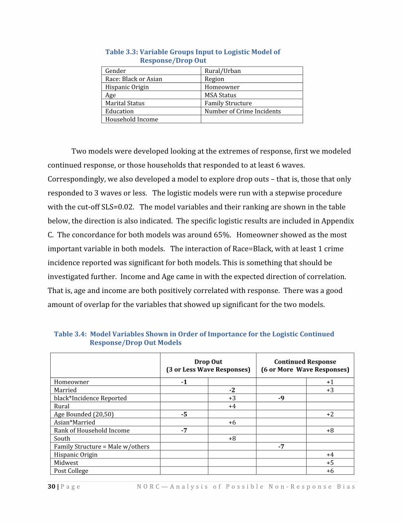
Table 3.3: Variable Groups Input to Logistic Model of Response/Drop Out
Gender Rural/UrbanRace: Black or Asian RegionHispanic Origin HomeownerAge MSA StatusMarital Status Family StructureEducation Number of Crime IncidentsHousehold Income
Two models were developed looking at the extremes of response, first we modeled
continued response, or those households that responded to at least 6 waves.
Correspondingly, we also developed a model to explore drop outs – that is, those that only
responded to 3 waves or less. The logistic models were run with a stepwise procedure
with the cut‐off SLS=0.02. The model variables and their ranking are shown in the table
below, the direction is also indicated. The specific logistic results are included in Appendix
C. The concordance for both models was around 65%. Homeowner showed as the most
important variable in both models. The interaction of Race=Black, with at least 1 crime
incidence reported was significant for both models. This is something that should be
investigated further. Income and Age came in with the expected direction of correlation.
That is, age and income are both positively correlated with response. There was a good
amount of overlap for the variables that showed up significant for the two models.
| P a g e N O R C — A n a l y s i s o f P o s s i b l e N o n ‐ R e s p o n s e B i a s 30
Table 3.4: Model Variables Shown in Order of Importance for the Logistic Continued Response/Drop Out Models
Drop Out
(3 or Less Wave Responses) Continued Response
(6 or More Wave Resp ses) on
Homeowner 1
+1Married 2 +3black*Incidence Reported +3 9 Rural +4Age Bounded (20,50) 5
+2
Asian*Married +6Rank of Household Income 7 +8South +8Family Structure = Male w/others 7
Hispanic Origin +4Midwest +5Post College +6

31 |
P a g e N O R C — A n a l y s i s o f P o s s i b l e N o n ‐ R e s p o n s e B i a s
3.4 Differential Response Rates and Dispositions by Subgroups
Although, the NCVS data collection is based on a longitudinal sample design with
the possibility of responding to the survey seven times in three and a half years, the NCVS
releases estimates and public use files with an annual focus. To reflect this we too focus on
annual response patterns. In particular, we investigate the data collected during 2002 and,
for a more recent comparison, 2007. Instead of focusing only on one cohort, which is
basically one‐sixth of the total sample, we are able to include much more data. For the
annual estimates, the selected units have the possibility of responding during January to
June, and then separately again during July to December. For analysis of patterns of
disposition outcomes, the entire annual data file is used. We also use the entire file for
general patterns of geographic41 and race for the Type A refusal nonresponse analysis. For
the more detailed socio‐crime related analysis which includes more detailed data collected
for the survey, we investigate the response pattern of those responding Jan-June and/or July-
December, for this analysis we only include the four cohorts that have the opportunity to respond
in both periods.42
We analyze the differential response by beginning at the top examining the
disposition patterns of sampled households and tunneling through to the detailed analysis
of individual respondents. At the top of the analyses is the detailing of the disposition
codes by the available geographic data – region, msa/not msa, place size, type of living
quarters and land use (rural/urban). The first level of response is at the sampled
household. As a benchmark, the resulting dispositions are compared for year 2002 and
2007 in terms of percent of total sampled units during January through December of the
respective year. There is about a 4% decrease in overall percentage of interviewed
household, almost half of this is due to an increase in the percent of vacant sampled units.
There were also small 0.5% increases in Type A reasons – No One at Home, Refusals and
Other. Overall the results appear fairly consistent for the two years. The detailed data is
included as Appendix Table C.3.8. Delving a bit deeper, we looked at disposition across
41 42 That is, we omit the cohort that is finishing up in the JanJune time frame, and the cohort that has its first
interview in the JulyDec timeframe.
Region, msa status, size of area, living quarters.

32 |
P a g e N O R C — A n a l y s i s o f P o s s i b l e N o n ‐ R e s p o n s e B i a s
geographic characteristics available on all sampled household units: region, land use, msa
status, place size code, type of living quarters. Disposition code has been collapsed to the
main categories. The results for urban/rural are shown in Table 3.5 below. There is a
pattern of higher refusals in urban areas, and more vacant units in rural areas.
Table3.5: ajor Disposition Outcomes for Sampled Units, by Urban/Rural M
Year 2002 Year 2007
Urban Rural Urban Rural
Type A No one home 2.06% 0.90% 2.33% 1.42%
Refused 4.11% 2.86% 5.01% 3.37%
Other Type A 1.05% 0.63% 1.39% 0.84%
Type B
Vacant‐regular 8.60% 14.60% 1 0.52% 1 5.95%
Other Type B 2.84% 6.73% 3.75% 6.62%
Type C
Demolished, converted to business 0.27% 0.58% 0.62% 1.11%
Interviewed Household 81.07% 73.70% 76.38% 70.68%
Dropping out the Type B and Type C units, we focus on responders and Type A non
responders. We are able to look at non response reason & responder results by these same
geographic variables with the addition of race (black/non‐black). The overall results are
shown in Table 3.6. Overall, blacks appear less responsive, with more “No One Home” and
“Refusals”.
Table 3.6: Response Outcomes for Black and Non Black for Year 2002 and 2007
Year 2002 Year 2007
Non Black Black Non Black Black Duplicate or Language problems 0% 0% 0 .08% 0 .08%No one home 1.9% 3.2% 2.4% 3.5% Temporarily absent 0.6% 0.6% 0.4% 0.3% Refused 4.4% 5.0% 5.5% 5.9% Other occupied 0.5% 0.5% 1.1% 1.3% Respond 92.6% 90.7% 90.5% 88.8% Total 100% 100% 100% 100%

33 |
P a g e N O R C — A n a l y s i s o f P o s s i b l e N o n ‐ R e s p o n s e B i a s
The response rates are shown separately for Region/black/nonblack in Table 3.7. Note
there is a lower response rate for blacks in the North East and West for the year 2002,
whereas the black response rate decreases for the Midwest region for 2007.
Table 3.7: Response Outcomes for Black/Non Black, by Region
Response Rate
2002 2007
North East Black 85% 85% No kn‐blac 90% 87%
Midwest Black 92% 86% No k n‐blac 94% 93%
South Black 93% 92% No k n‐blac 94% 92%
West Black 85% 83%
Non‐black 91% 89%
The lower response rate for the blacks in the Northeast and Midwest appears to be
mainly due to low response in urban areas for those regions, as shown in Chart 3.4 below
where response rate is graphed against percent of sample. Each point represents a group
identified by Region, Urban/Rural, and Black/nonblack. The two points in the lower left
corner, show the much lower response rate obtained for Black respondents in the
Northeast and West urban areas.

34 |
P a g e N O R C — A n a l y s i s o f P o s s i b l e N o n ‐ R e s p o n s e B i a s
Chart 3.4: Response Rate by Percent of Sample, 2002
3.5 More on Responder Differences
We now turn to look at the differences in responders, where we have more detailed
data as well as survey outcomes that allows a more intense view of the impacts of
differential nonresponse. The question at this point becomes, what differential not missing
at random non response remains that can be accounted for with models or other factors
based on prior waves response.
The Public Use Files are structured to allow analysts to compute annual estimates,
either in a collection year, or as the data year. We are working with the two waves that are
put together to compute estimates for a collection year. Sampled units have an option of

responding to either the first or second, or preferably, to both waves in a given year. To
get a feeling for the patterns, we first examine patterns of responding households for the
data collection year. Response pattern per wave 1 and wave 2 by income is shown below in
Chart 3.5, the corresponding graph by Education is included as Appendix Table C.3.11.
Chart 3.5: Percent Responding Households by Income, 2002
One method to examine the response impact, is to compute the restricted estimates
by the response pattern (Jan‐June only, both Jan‐June & July‐Dec, and July – Dec only)
results, shown in Table 3.8 below, are based only on those households with the possibility
of responding in both Jan‐June and July‐Dec 2002. That is, like the above graphs, the panels
that were being rotated out or rotated in are not included.43 There is not a noticeable
difference in the restricted estimates for the different groups of responders.
35 | P a g e N O R C — A n a l y s i s o f P o s s i b l e N o n ‐ R e s p o n s e B i a s
43 The population percentages, and the proportion of crime reported are weighted estimates, using the
collection year weight available on the public use file.

36 | P a g e N O R C — A n a l y s i s o f P o s s i b l e N o n ‐ R e s p o n s e B i a s
Table 3.8: Restricted Results for Annual 2002 Estimates: Proportion of Households Reporting Crime Incident
Nonresponse Respond July‐Dec July‐Dec
Nonresponse % population 2% Jan‐June
Crime Incident 0 .0867R esponse 3% 94% Jan‐June
0.0920 0.0842
Using the more detailed data on the responders, we develop logistic regression
models to predict nonresponse. In this situation, we separate the annual file into
responders (responded in both time periods) and nonresponders (did not respond in one
time period). We develop models for both 2002 and 2007. The results are similar as those
where we used all of the wave responses to predict drop outs, or loyal responders. The
concordance for the 2002 model is 62.7, for the 2007 model it is slightly higher at 68.7.
One must note that there are 8% nonresponders in the 2002 data, and 14.5% for 2007.
This difference is because the first (the unbounded) interview is included for analysis on
the later public use file.44 The logistic regression results are shown in Appendix Tables
C.3.10 and 45C.3.11.
Stepping back from the detailed file, we consider broader patterns of nonresponse,
including the Type A refusals, and their relationship to victimization estimates. The
pattern in Chart 3.6 suggests something we already saw in our modeling work in Chapter 2;
that it is plausible to believe that much of the nonresponse is not biasing. In Chapter 2 we
assessed this from a process perspective. Here we are looking at refusal rates by crime
rates and see little pattern. Again we caution against overpromising relative to low bias for
the NCVS but consider the outcome encouraging. One last point: The nonresponse rate
from the first round is not included for the 2002 results, but in the later public use files
44 Beginning in 2006, the first bounding interviews are included on the Public Use Files. 45 Another possible method for addressing nonresponse is to impute missing units using their prior
survey data. Such an analysis was performed, the results are shown in Appendix Table C.3.12.
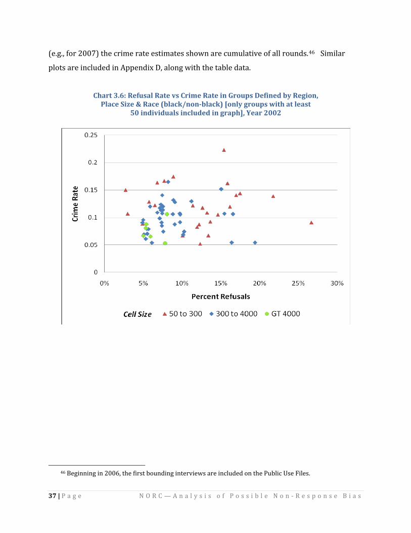
(e.g., for 2007) the crime rate estimates shown are cumulative of all rounds.46 Similar
lots are included in Appendix D, along with the table data. p
Chart 3.6: Refusal Rate vs Crime Rate in Groups Defined by Region, Place Size & Race (black/nonblack) [only groups with at least
50 individuals included in graph], Year 2002
37 | P a g e N O R C — A n a l y s i s o f P o s s i b l e N o n ‐ R e s p o n s e B i a s
46 Beginning in 2006, the first bounding interviews are included on the Public Use Files.

38 |
P a g e N O R C — A n a l y s i s o f P o s s i b l e N o n ‐ R e s p o n s e B i a s
Chapter 4
An Analysis of the NCVS and UCR Crime Statistics
at the CountyLevel, 20032006
4.1 Introduction
The U.S. Department of Justice administers two statistical programs to measure the
magnitude, nature, and impact of crime in the Nation: the Uniform Crime Reporting (UCR)
Program and the National Crime Victimization Survey (NCVS). The UCR and the NCVS differ
in that they “are conducted for different purposes, use different methods, and focus on
somewhat different aspects of crime.”47 So inevitably there are discrepancies between
estimates derived from these two different measures of crime. Nonetheless, “long‐term
[NCVS and UCR] trends can This is not surprising in be brought into close concordance” by
analysts familiar with the programs and data sets48 that the NCVS was designed “to
complement the UCR program.”49 So while the NCVS and UCR programs each were
designed to collect different data, each offers data that are criminologically relevant, and
together they “provide a more complete assessment of crime in the United States” 50 than
either c 51ould produce alone.
The conclusion that both surveys are essential to the measurement of crime in the
United States underscores the importance of the current request by BJS for proposals to
conduct methodological research to support a present‐day redesign of the NCVS.52 More
broadly, these are challenging times for survey research generally given dramatic and fast‐
47 BJS 2004:1. Bureau of Justice Statistics. 2007. National Crime Victimization Survey: MSA Data, 1979
2004 om uter fi e]. Ann Arbor, MI: Inter‐University Consortium for Political and Social Research. [ lC p48 BJS 20042 49 ibid. 50 Lauritsen, J.L. and Schaum, R.J. 2005. “Crime and Victimization in the Three Largest Metropolitan Areas,
198098.” Washington, D.C.: Bureau of Justice Statistics, http://www.ojp.usdoj.gov/bjs/pub/pdf/cv3lma98.pdf (accessed September 30, 2009).
51 on, 2008.” Washington, D.C.: U.S. Bureau of Justice Statistics, Rand, M. R. 2009.” Criminal Victimizati//www.ojp.usdoj.gov/bjs/pub/pdf/cv08.pdfhttp: (acce52 Federal Bureau of Investigation. 2008. The Nation’s Two Crime Measures. Uniform Crime Report, Crime
in the United States, 2007.” Washington, D.C.: U.S.,
ssed on October 4, 2009).
http://www.fbi.gov/ucr/cius2007/documents/crime_measures.pdf (accessed on October 4, 2009).

39 | P a g e N O R C — A n a l y s i s o f P o s s i b l e N o n ‐ R e s p o n s e B i a s
paced technological, social, and cultural change. It is also challenging how the UCR data
may fac 53ilitate in improving the NCVS estimation counts at the local level.
In order to better understand and utilize the relationship between the NCVS and
UCR at the sub‐national level, we examined the NCVS crime victimization estimates and the
UCR arrest. Specifically, we attempted to estimate the victimization totals at the county
level and compare all the NCVS county estimates with the count records from the UCR. For
illustration, we focused on the 2003‐2006 period, used four‐year pooled NCVS and UCR,
and examined summated measures of victimizations and crimes so that the NCVS and UCR
measures can be better comparable.
The National Crime Victimization Survey (NCVS) Series, previously called the
National Crime Surveys (NCS), has been collecting data on personal and household
victimization through an ongoing survey of a nationally‐representative sample of
residential addresses since 1973. During the 2003‐2006, household residents from all the
50 states plus the Districtrict of Columbia participated in the surveys. There are wide
variations in terms of the numbers of the counties that were in the NCVS samples in this
period. The top five states with the largest number of counties involved in the NCVS data
collections were Texas (52 Counties), Virginia (47 counties), Ohio (44 counties), Georgia
(39 counties), and New York (37 counties). Only one county within the following states had
residents participating in NCVS during 2003‐2006: Hawaii, New Hampshire, Vermont, and
Wyoming.
4.2 Data Sources
This analysis examined the differences and the relationships at the county level
between the National Crime Victimization Surveys and the Uniform Crime Reports (UCR) in
the period of 2003‐2006. New weights were developed for this analyses so that the
county‐level annual NCVS estimations of the totals can be produced. UCR information were
53 McDowall, D. and C. Loftin, C. 2007. “What Is Convergence and What Do We Know About It?” in
Understanding Crime Statistics: Revisiting the Divergence of the NCVS and UCR, eds. J. P. Lynch and L. A. Addingtion. New York: Cambridge University Press.

40 | P a g e N O R C — A n a l y s i s o f P o s s i b l e N o n ‐ R e s p o n s e B i a s
retrieved from the annualized county‐level UCR data only for those counties in the NCVS
samples in the same year. (See Appendix E, tables E4.1‐E4.4.)
Because the BJS designed the NCVS to complement the UCR Program, the two
programs share many similarities. As much as their different collection methods permit,
the two measure the same subset of serious crimes, defined alike. Both programs cover
rape, robbery, aggravated assault, burglary, theft, and motor vehicle theft. Rape, robbery,
theft, and motor vehicle theft are defined virtually identically by both the UCR and the
NCVS. (Although rape is defined analogously, the UCR Program measures the crime against
women only, and the NCVS measures it against both sexes.)
There are significant differences between the two programs: (1) the two programs
were created to serve different purposes; (2) the two programs measure an overlapping
but nonidentical set of crimes; (3) The NCVS includes crimes both reported and not
reported to law enforcement. The NCVS excludes, but the UCR includes, homicide, arson,
commercial crimes, and crimes against children under age 12. The UCR captures crimes
reported to law enforcement but collects only arrest data for simple assault and sexual
assault other than forcible rape. (3) the NCVS and UCR definitions of some crime differ. For
example, the UCR defines burglary as the unlawful entry or attempted entry of a structure
to commit a felony or theft. The NCVS, not wanting to ask victims to ascertain offender
motives, defines burglary as the entry or attempted entry of a residence by a person who
had no right to be there. 54
4.3 Measurement
The National Crime Victimization Survey covers all of the index offenses covered by
the Uniform Crime Reports, except for homicide and arson. Therefore, when comparing the
total counts of crime victimizations and arrests, we exclude murder and arson from the
UCR total count measure.
54 Federal Bureau of Investigation. 2008. “Crime in the United States, 2008 .” Washington, D.C.: U.S. Federal
Bureau of Investigation, 2008, http://www.fbi.gov/ucr/cius2008/about/index.html (accessed on October 4, 2009).

41 |
P a g e N O R C — A n a l y s i s o f P o s s i b l e N o n ‐ R e s p o n s e B i a s
Due to skewed distributions of the untransformed raw counts and “outliers” found
in the scatterplots, separate alternative scatterplots were made using the logarithm
transformations of the crime totals (log(counts +1)). Further scatterplots were shown with
some peculiar counties (i.e., counties with no crime victimization reported, that is, NCVS
county level crime incident count=0, and counties with no arrest reported, that is, UCR
county level arrest count=0 for the 2003‐2006 period) excluded.
In this analysis, the crimes included in the totals from the NCVS included: Rape,
Robbery, Assault, Burglary, Motor Vehicle Theft, Purse Snatching, and Theft; and the crimes
included in the totals from the UCR included: Rape, Robbery, Assault, Burglary, Motor
Vehicle Theft, and Larceny.
During 2003‐2006, of all the counties where NCVS data were collected, a total of 46
counties showed zero number of arrests. All these 46 counties had considerable large
amount of crime victimization incident reports in the same time period (see Table E4.5). A
total of 56 counties had zero crime victimization incidents reported during 2003‐2006,
although many of them made many arrests for criminal offenses (see Table E4.6).
4.4 Results
Estimations and counts were obtained for each of the four years in 2003‐2006. The
combined totals at the county level were thereafter obtained through the summations of
the year‐specific totals in NCVS and UCR respectively. Only the results for the combined
2003‐2006 are shown here. The year‐specific scatter plots are also available in the NORC
workpapers and appendices.
Figure 1 shows the scatter plot of the total victimizations in NCVS by the total
crimes in UCR. Significant positive relationship was observed. The R2 of the linear
regression model was 0.80.

42 |
P a g e N O R C — A n a l y s i s o f P o s s i b l e N o n ‐ R e s p o n s e B i a s
As the distribution of the victimization counts at the county level appears to be
skewed, we made a logarithmic transformation on the outcomes without dropping any
ases. Figure 2 shows the scatter plot. c
Because of the logarithm transformations of the crime totals (log(counts +1)),
counties with zero count of victimizations could still be shown; actually, the scatter plot in
Figure 2 demonstrated that there were quite a few zero‐type of counties from both NCVS

43 |
P a g e N O R C — A n a l y s i s o f P o s s i b l e N o n ‐ R e s p o n s e B i a s
and UCR. Not surprisingly, the R2 as a fit statistics of the regression model dropped
dramatically due to these outliers.
4.5 Outliers
The counties with either victimization counts being zero or crime arrest counts
being zero – were carefully examined next. Of course, these zero‐counties are only an
example of the data problems that a careful analysis might find
1. UCR “zerotype “counties. Among all the counties where NCVS data were collected during 2003‐2006, a total of 46 counties were found to have “zero” number of arrests for any of the six major index crimes (murder was excluded). As shown in Table 4.1, 3/5 of these counties were located in the State of Florida, and 1/3 of hese counties were located in the State of Illinois. Minnesota and Virginia each ad one “zero‐type” countth y.
2. NCVS “zerotype” counties. During 2003‐2006, there existed 55 counties where NCVS data were collected but there were no victimization incidents reported. Virginia had the largest number of “zero‐type” of counties (n=12), followed by Texas (n=6), Louisiana (n=4). Table 4.2 list all states which had at least one “zero‐type” county.
Table 4.1: Distribution of Counties Where UCR Crime Counts During 2003 – 2006 Were Zero
State Frequency Pe nt rce
Florida 28 61 Illinois 1 6 35 Minnesota 1 2 Virginia 1 2 ALL 46 100
Table 4.2: Number of Counties Where NCVS Crime Counts During 2003 – 2006 Were Zero, by State
State Frequency Number of Total nties C uo
Virginia 1 2 1 2Texas 6 6Louisiana 4 4Colorado, Georgia, Missouri, Tennessee 3 12Iowa, Kentucky, Mississippi, Wisconsin 2 8AlaMe
bama, Illinois, Indiana, Michigan, Minnesota, Nebraska, Nevada, New xico, New York, North Carolina, Oklahoma, Pennsylvania, Utah 1 14
All 56

44 |
P a g e N O R C — A n a l y s i s o f P o s s i b l e N o n ‐ R e s p o n s e B i a s
Did the UCR “zero‐type” counties have larger than 0 amount of victimization
incidents reported in NCVS? or vice versa? The answer is yes to both. Details, including the
counties involved are shown in the Appendix Tables E4.5 and E4.6, whereas the
inconsistencies found between the UCR and NCVS may need further investigations, we
excluded these “zero‐type” counties from the subsequent analyses.
4.6 Relationship between the NCVS and UCR
Figure 4.3 shows the scatter plot of the total victimizations in NCVS by the total
crimes in UCR among the counties which had non‐zero amount of victimization incidents
and criminal offense arrests.
Figure 4.3: Scatterplot of the Total Crime Counts, NCVS by UCR, for Counties
Which Had At Least One Victimmization Incident and One Official Arrest,
at the County Level, 20032006
Figure 3a: Raw Totals Figure 3b: Logarithm of Raw Total

Figure 4.4: Logarithms of Total Counts of Crime Incidents – NCVS by UCR,
in 2003 – 2006, By Region
Excluding counties where total victimization incident count =0 or arrest count =0
Figure 4.4 shows the scatter plots of the log transformations of the NCVS
victimization incident count by UCR arrest count for each of the four regions separately.55
Strong positive significant relationships were observed for each of the four regions.
Table 4.3 shows a summary of the R‐squares in the linear regression models with
the weighted estimations of the total counts of the crime victimization incidents reported
in NCVS as the dependent variable and the total counts of arrests reported by the county‐
level UCR as the independent variable.
45 | P a g e N O R C — A n a l y s i s o f P o s s i b l e N o n ‐ R e s p o n s e B i a s
55 Region‐specific scatter plots on raw totals, region‐specific scatter plots on raw totals with zero‐type
outliers excluded, and region‐specific scatter plots on log transformations with raw totals are listed in the Appendix B, Tables B4.1‐B4.3.

46 | P a g e N O R C — A n a l y s i s o f P o s s i b l e N o n ‐ R e s p o n s e B i a s
Table 4.3: Rsquares in the regression analysis of the Arrests Reported by UCR and the Crime
Victimizations Captured by the NCVS
Crimes ALL Region
No strthea M tidwes South West Total crime 0.80 0.660 0.898 0.653 0.929Logarithm of total crime counts 0.283 0.602 0.338 0.132 0.694Total crime with restrictions to Total Victimization and Crime > 0 0.821 0.658 0.903 0.747 0.928
Logarithm of total crime counts with restrictions to Total Victimization and Crime > 0
0.828 0.815 0.827 0.765 0.945
Note: In the regression models depicted by the scatter plots, the square root of R‐square is the same as the correlation coefficients. Overall, and across each of the census regions, the correlations (r) between the NCVS estimates and the UCR estimates are very high. The R2 was 0.828 (r=.9+) at the national level, and ranged from 0.765 (r= +.8) to 0.945 (r= +.95) at the regional level.
There are variations across the four census regions in terms of the extent the
magnitudes of the UCR arrest counts can explain the variability of the crime victimizations
reported by householders. Regardless whether we transformed the crime and victimization
counts or whether we eliminated the outliers such as those counties which had no or
extremely high level of victimizations, the West Region had the highest level of R2. (i.e., R2 =
.929 before any transformation and truncation; R2 = .945 after the exclusion of outliers and
the transformation).
In the past, the UCR and the NCVS have been used at the national level to assess
their correlations on specific index crimes (BJS, 2007; Lauritsen and Schaum, 2005;
McDowall and Loftin, 2007). Both high and low correlations have been observed. A high
correlation between UCR and NCVS trends would suggest that either data series would
serve as a reasonable proxy for some analytical purposes (NRC, 2008:72). In addition to
definitional difference on certain crimes (FBI, 2008), there are conjectures on what would
make the UCR and NCVS differ such as the matters concerning the public’s willingness to
report crime to the police and the way police departments record crime, how these factors
may vary across regions or other geographic units remains an important questions that
hall need further investigation which is beyond the scope this study. s

47 | P a g e N O R C — A n a l y s i s o f P o s s i b l e N o n ‐ R e s p o n s e B i a s
Chapter 5
Summary and Recommendations
5.1 Summary
In this report we stated a number of working hypotheses about unit nonresponse
(Chapter 1) and then set out to test some of them (Chapters 2 and 3). Chapter 4 was
devoted mainly to the possible joint use of the NCVS, with the uniform crime reports (UCR).
Scope limitations restricted us mainly to exploratory methods on NCVS rounds after
the first. We could not analyze nonresponse in the first round directly. Confirmatory results
were not obtained but several results were suggestive of what a fuller analysis might find.
Bottom line, there was little evidence for nonresponse bias after the first round of
the survey. Chapters 2 and 3 had information suggestive of this at the household level. In
an appendix to Chapter 3, we display a logistic regression to characterize the person level
nonresponse. Here, in this regression, we do find some evidence of differential
nonresponse that might be biasing, if not addressed. However, the person level
nonresponse is weight adjusted to age and race controls in the NCVS and these seem to be
the categories that are the main drivers in any potential nonresponse bias.
5.2 Recommendations for Immediate Action
We have repeatedly expressed concerns about the first round being potentially
biasing. A discussion of this and two other process recommendations are highlighted
elow.b
56
56 We have, however, yet to address systematically the suggestions BJS wanted us to look at. These will be
covered in our briefing later this month.

48 |
P a g e N O R C — A n a l y s i s o f P o s s i b l e N o n ‐ R e s p o n s e B i a s
Nonresponse during first attempted contact. The literature on panel surveys
cited earlier suggests that the first round is where the potential for
nonresponse bias is the most severe, largely because there are so few
covariates to model and adjust with.57 Doing more here in the NCVS,
especially adding to the frame seems an obvious action step. Bringing
forward additional data from the UCR or the previous census would be good.
A close examination of the paradata picked up when there is a noncontact or
a refusal in the first round outcome might be made. In NORC’s Survey of
Consumer Finances, for example, neighborhood information is obtained.
Some pairing of cases ahead of time, e.g., having two linked interviews in the
same ultimate cluster could be a sensible precaution for household, person,
and item nonresponse.
Reinterviews to check on response quality and nonresponse bias. The scope of
the NORC proposal kept us from looking at the Census Bureau’s reinterview
program. We would recommend time be spent studying how successful this
effort is and whether it could be harnessed to study a small sample of
nonresponse cases from each round of the NCVS, especially but not
exclusively the first round.58 Since the focus will be on bias examination a
very high response rate will be needed for these reinterviews, making this an
expensive undertaking in time and money. To limit the effort, a real‐time MIS
might be set up and results posted routinely. Stopping rules could be
developed after the program started and after efforts to optimize resources
were attempted.
Imputation Experiments. In Chapter 1 we mentioned ideas about how to plan
and carryout nonresponse adjustments that were mixtures of reweighting
and imputation. These seem to offer the best general approach to NCVS
57 With only a limited number of covariates the nonresponse may, ceteris paribus, be more often
nonignorable. 58 BJS already has staff conversant in such methods and their limitations (e.g., Sinclair, M.D. 1994.
“Evaluating Reinterview Survey Methods for Measuring Response Errors,” (Ph.D. dissertation, George Washington University).

49 | P a g e N O R C — A n a l y s i s o f P o s s i b l e N o n ‐ R e s p o n s e B i a s
missingness, whether of whole households, persons or individual items. This
too should be tried in a limited way.
In Appendix G six broad areas are covered: (1) Paradata construction and related
issues. (2) Longitudinal NCVS Constructions and Related Analyses, (3) Addressing bias and
variance reduction, (4) Bounding procedures, (7) Examining the organization of crime
event information and (6) Design Elements. These might be addressed here but will not.
Instead, they will be taken up selectively when NORC and BJS get together later this
month.59
59 The three suggestions that BJS considered useful in the short term were (1) Improving paradata
construction and related interviewer information, (2) Improving information related to contact with respondents and (3) Analyses of longitudinal cohorts.

Appendix A
P a g e N O R C — A n a l y s i s o f P o s s i b l e N o n ‐ R e s p o n s e B i a s
Table A2.1: CaptureRecapture Analyses of Household Cohort 11 Refusals across Waves
Wave Wave by a b c d di=bc/a u=(ddi) [u 2 /d]*100 [u /(a+b+c+d)]*100 [u/( 100 b+c+d)]*
ic12 150 147 157 6375 153.86 6221.14 97.6% 91.099% 93.145% ic13 122 174 219 6415 312.34 6102.66 95.1% 88.061% 89.639% ic14 108 190 252 6328 443.33 5884.67 93.0% 85.558% 86.923% ic15 101 171 287 5825 485.91 5339.09 91.7% 83.632% 84.977% ic16 82 185 279 5448 629.45 4818.55 88.4% 80.390% 81.505% ic17 41 133 188 3743 609.85 3133.15 83.7% 76.325% 77.095% ic23 169 135 170 6519 135.80 6383.20 97.9% 91.280% 93.540% ic24 150 155 216 6402 223.20 6178.80 96.5% 89.250% 91.227% ic25 127 142 265 5848 296.30 5551.70 94.9% 86.990% 88.756% ic26 110 162 253 5477 372.60 5104.40 93.2% 85.045% 86.633% ic27 60 119 175 3744 347.08 3396.92 90.7% 82.892% 84.124% ic34 193 140 168 6488 121.87 6366.13 98.1% 91.088% 93.675% ic35 156 144 237 5913 218.77 5694.23 96.3% 88.283% 90.471% ic36 129 163 232 5499 293.15 5205.85 94.7% 86.433% 88.325% ic37 81 134 153 3764 253.11 3510.89 93.3% 84.968% 86.667% ic45 209 125 192 6000 114.83 5885.17 98.1% 90.180% 93.164% ic46 174 147 190 5564 160.52 5403.48 97.1% 88.946% 91.569% ic47 94 116 137 3795 169.06 3625.94 95.5% 87.541% 89.574% ic56 218 156 143 5556 102.33 5453.67 98.2% 89.802% 93.146% ic57 118 122 107 3805 110.63 3694.37 97.1% 88.978% 91.581% ic67 144 92 85 3850 54.31 3795.69 98.6% 91.002% 94.256%
Note: a. Count of refusal households in both designated waves b. Count of households refusing in the first designated wave but not in the second designated wave c. Count of households refusing in the second designated wave but in the first designated wave d. Count of eligible households not refusing in both designated waves 1Based on households in cohort 1 with the first rotation in the sample in the first 6 month in 2003 2Percentages in this column denote the percentages of potentially nonignorable missing households Source: NCVS 2003‐2006 Longitudinal File
50 |

Table A2.2: CaptureRecapture Analyses of Household Cohort 21 Refusals across Waves
Wave by Wave a b c d di=bc/d u=(ddi) [u/d]*100 2 [u /(a+b+c+d)]*100 [u/( 100 b+c+d)]*
ic12 145 154 143 6620 151.88 6468.12 97.7% 91.591% 93.511% ic13 118 171 221 6390 320.26 6069.74 95.0% 87.967% 89.498% ic14 96 181 252 5931 475.13 5455.88 92.0% 84.456% 85.730% ic15 80 176 255 5562 561.00 5001.00 89.9% 82.348% 83.447% ic16 58 115 218 3569 432.24 3136.76 87.9% 79.211% 80.388% ic17 45 131 177 3643 515.27 3127.73 85.9% 78.272% 79.163% ic23 158 118 172 6513 128.46 6384.54 98.0% 91.719% 93.849% ic24 118 147 223 6029 277.81 5751.19 95.4% 88.249% 89.876% ic25 94 150 236 5616 376.60 5239.40 93.3% 85.948% 87.294% ic26 67 95 205 3600 290.67 3309.33 91.9% 83.421% 84.855% ic27 50 111 165 3669 366.30 3302.70 90.0% 82.671% 83.719% ic34 170 138 171 6067 138.81 5928.19 97.7% 90.562% 92.977% ic35 136 143 195 5627 205.04 5421.96 96.4% 88.870% 90.896% ic36 92 105 178 3623 203.15 3419.85 94.4% 85.539% 87.554% ic37 69 119 149 3663 256.97 3406.03 93.0% 85.151% 86.645% ic45 183 133 152 5700 110.47 5589.53 98.1% 90.621% 93.392% ic46 111 105 158 3618 149.46 3468.54 95.9% 86.887% 89.372% ic47 92 124 126 3645 169.83 3475.17 95.3% 87.163% 89.221% ic56 148 82 126 3704 69.81 3634.19 98.1% 89.512% 92.898% ic57 108 112 105 3705 108.89 3596.11 97.1% 89.234% 91.691% ic67 144 130 72 3724 65.00 3659.00 98.3% 89.902% 93.199%
Note: a. Count of refusal households in both designated waves b. Count of households refusing in the first designated wave but not in the second designated wave c. Count of households refusing in the second designated wave but in the first designated wave d. Count of eligible households not refusing in both designated waves 1Based on households in cohort 2 with the first rotation in the sample in the second 6 month in 2003 2Percentages in this column denote the percentages of potentially nonignorable missing households Source: NCVS 2003‐2006 Longitudinal File
51 | P a g e N O R C — A n a l y s i s o f P o s s i b l e N o n ‐ R e s p o n s e B i a s

Table A2.3: CaptureRecapture Analyses of Household Cohort 11 Other Type A across Waves
Wave Wave by a b c d di=bc/a u=(ddi) [u 2 /d]*100 [u /(a+b+c+d)]*100 [u/( 100 b+c+d)]*
ic12 24 273 248 6484 2821.00 3663.00 56.5% 52.113% 52.291% ic13 22 274 210 6424 2615.45 3808.55 59.3% 54.957% 55.132% ic14 20 278 202 6378 2807.80 3570.20 56.0% 51.908% 52.059% ic15 15 257 212 5900 3632.27 2267.73 38.4% 35.522% 35.606% ic16 12 255 181 5546 3846.25 1699.75 30.6% 28.358% 28.414% ic17 13 161 126 3805 1560.46 2244.54 59.0% 54.678% 54.852% ic23 22 282 207 6482 2653.36 3828.64 59.1% 54.750% 54.922% ic24 28 277 200 6418 1978.57 4439.43 69.2% 64.126% 64.386% ic25 14 255 215 5898 3916.07 1981.93 33.6% 31.055% 31.123% ic26 13 259 183 5547 3645.92 1901.08 34.3% 31.674% 31.743% ic27 13 166 117 3802 1494.00 2308.00 60.7% 56.320% 56.499% ic34 18 315 200 6456 3500.00 2956.00 45.8% 42.295% 42.404% ic35 13 287 213 5937 4702.38 1234.62 20.8% 19.141% 19.180% ic36 16 276 169 5562 2915.25 2646.75 47.6% 43.944% 44.061% ic37 20 195 114 3803 1111.50 2691.50 70.8% 65.138% 65.455% ic45 17 317 209 5983 3897.24 2085.76 34.9% 31.961% 32.044% ic46 12 309 183 5571 4712.25 858.75 15.4% 14.136% 14.164% ic47 17 193 119 3813 1351.00 2462.00 64.6% 59.440% 59.685% ic56 24 350 163 5536 2377.08 3158.92 57.1% 52.016% 52.222% ic57 19 128 119 3793 801.68 2991.32 78.9% 73.696% 74.042% ic67 18 218 115 3820 1392.78 2427.22 63.5% 58.193% 58.445%
Note: a. Count of other type A households in both designated waves b. Count of households being other type A in the first designated wave but not in the second designated wave c. Count of households being other type A in the second designated wave but in the first designated wave d. Count of eligible households not being type A in both designated waves 1Based on households in cohort 1 with the first rotation in the sample in the first 6 month in 2003 2Percentages in this column denote the percentages of potentially nonignorable missing households Source: NCVS 2003‐2006 Longitudinal File
52 | P a g e N O R C — A n a l y s i s o f P o s s i b l e N o n ‐ R e s p o n s e B i a s

Table A2.4: CaptureRecapture Analyses of Household Cohort 21 Other Type A across Waves
Wave Wave by a b c d di=bc/d u=(ddi) [u/d]*100 2 [u /(a+b+c+d)]*100 [u/( 100 b+c+d)]*
ic12 30 269 217 6546 1945.77 4600.23 70.3% 65.141% 65.419% ic13 21 268 223 6388 2845.90 3542.10 55.4% 51.335% 51.491% ic14 19 258 247 5936 3354.00 2582.00 43.5% 39.969% 40.087% ic15 17 239 222 5595 3121.06 2473.94 44.2% 40.737% 40.851% ic16 6 167 129 3658 3590.50 67.50 1.8% 1.705% 1.707% ic17 10 166 107 3713 1776.20 1936.80 52.2% 48.468% 48.590% ic23 22 254 219 6466 2528.45 3937.55 60.9% 56.566% 56.745% ic24 21 244 242 6010 2811.81 3198.19 53.2% 49.075% 49.233% ic25 15 229 215 5637 3282.33 2354.67 41.8% 38.626% 38.722% ic26 5 157 135 3671 4239.00 ‐568.00 ‐15.5% ‐14.315% ‐14.333% ic27 10 151 110 3724 1661.00 2063.00 55.4% 51.640% 51.769% ic34 28 280 225 6013 2250.00 3763.00 62.6% 57.485% 57.732% ic35 24 255 211 5611 2241.88 3369.13 60.0% 55.223% 55.441% ic36 8 189 136 3665 3213.00 452.00 12.3% 11.306% 11.328% ic37 14 174 100 3712 1242.86 2469.14 66.5% 61.729% 61.945% ic45 20 296 216 5636 3196.80 2439.20 43.3% 39.546% 39.675% ic46 11 205 130 3646 2422.73 1223.27 33.6% 30.643% 30.728% ic47 14 202 98 3673 1414.00 2259.00 61.5% 56.659% 56.859% ic56 15 215 123 3707 1763.00 1944.00 52.4% 47.882% 48.059% ic57 13 207 100 4058 1592.31 2465.69 60.8% 56.320% 56.488% ic67 22 252 93 3703 1065.27 2637.73 71.2% 64.809% 65.161%
Note: a. Count of other type A households in both designated waves b. Count of households being other type A in the first designated wave but not in the second designated wave c. Count of households being other type A in the second designated wave but in the first designated wave d. Count of eligible households not being type A in both designated waves 1Based on households in cohort 2 with the first rotation in the sample in the second 6 month in 2003 2Percentages in this column denote the percentages of potentially nonignorable missing households Source: NCVS 2003‐2006 Longitudinal File.
53 | P a g e N O R C — A n a l y s i s o f P o s s i b l e N o n ‐ R e s p o n s e B i a s

Appendix B
Table B2.1: Capture – Recapture Analysis of the NCVS NonResponses Among 2003 Cohort 1 ALL Household Respondents
W 1)aves (t by t+ Interviewed at Bo avesth W
Interviewed at Wave t but not Wa +1 ve t
Interviewed at Wave t+1 bu t t t No
Type A Nonresponses at Both t and
t+1 Expected (Modeled) Value of
Type A sponse NonreActual > Mo d? dele
Percent Di ce fferen
t=1 by t+1=2 6156 294 304 275 14.52 yes 94.72 t=2 by t+1=3 6134 185 289 92 8.72 yes 90.53 t=3 by t+1=4 6142 171 288 97 8.02 yes 91.73 t=4 by t+1=5 5685 138 329 95 7.99 yes 91.59 t=5 by t+1=6 5250 193 251 86 9.23 yes 89.27 t=6 by t+1=7 3646 111 156 51 4.75 yes 90.69 All t by (t+1) 33013 1092 1617 696 53.22 yes 92.35
Total ignorable (1092+1617+53)=2762
% of nonresponse that is ignorable 2762/(1092+1617+696)=81.1%
Waves
(t by t+1)
t=1 by t+1=2
Type A Nonresponses at Bot nd t+1 h t a
275
Never
Interviewed Again
Interviewed
at Le Once ast
96
Percent Returned to be Interviewed
34.9 179 t=2 by t+1=3 92 39 53 57.6 t=3 by t+1=4 97 48 49 50.5 t=4 by t+1=5 95 61 34 35.8 t=5 by t+1=6 86 70 16 18.6 All t by (t+1) 645 397 248 38.4
54 | P a g e N O R C — A n a l y s i s o f P o s s i b l e N o n ‐ R e s p o n s e B i a s

Table B2.2: Capture – Recapture Analysis of the NCVS NonResponses Among 2003 Cohort 1 MALE Household Respondents
Waves
(t by t+1) Interviewed at b ves oth wa
Interviewed at wave t but not
e t+1 wav
Interviewed at wave t+1 ut not t b
Type A Nonresponses at bo and t+1 th t
Expected (modeled) value of Type A
Nonresponse
Actual > Mo d? dele
Percent Di ce fferen
t=1 by t+1=2 3288 105 166 71 5.30 yes 92.53 t=2 by t+1=3 3223 100 130 50 4.03 yes 91.93 t=3 by t+1=4 3212 75 147 48 3.43 yes 92.85 t=4 by t+1=5 2967 78 161 42 4.23 yes 89.92 t=5 by t+1=6 2747 94 122 41 4.17 yes 89.82 t=6 by t+1=7 1855 49 77 23 2.03 yes 91.16 All t by (t+1) 17292 501 803 275 23.21 yes 91.56
Total ignorable (501+803+23)=1327
% of nonresponse that is ignorable (501+803+23)/(501+803+275)=84.04%
Waves
(t by t+1)
t=1 by t+1=2
Type A Nonresponses at Both t d t+1 an
71
Never
Interviewed Again
Interviewed
at Le Once ast
42
Percent Returned to be Interviewed
59.2 29 t=2 by t+1=3 50 26 24 48.0 t=3 by t+1=4 48 26 22 45.8 t=4 by t+1=5 42 27 15 35.7 t=5 by t+1=6 41 38 3 7.3 All t by (t+1) 252 146 106 42.1
55 | P a g e N O R C — A n a l y s i s o f P o s s i b l e N o n ‐ R e s p o n s e B i a s

Table B2.3: Capture – Recapture Analysis of the NCVS NonResponses Among 2003 Cohort 1 FEMALE Household Respondents
Waves
(t by t+1) Interviewed at Both waves
Interviewed at Wave t but not Wa +1 ve t
Interviewed at Wave t+1 bu t t t no
Type A Nonresponses at Both t and
t+1
Expected (modeled) Value of Type A
Nonresponse
Actual > Modeled?
Percent Difference
t=1 by t+1=2 2868 189 138 98 9.09 yes 90.72 t=2 by t+1=3 2911 85 159 42 4.64 yes 88.95 t=3 by t+1=4 2930 96 141 49 4.62 yes 90.57 t=4 by t+1=5 2718 60 168 53 3.71 yes 93.00 t=5 by t+1=6 2503 99 129 45 5.10 yes 88.66 t=6 by t+1=7 1791 62 79 28 2.73 yes 90.23 All t by (t+1) 15721 591 814 315 29.90 yes 90.51
Total ignorable (591+814+30)=1435
% of nonresponse that is ignorable (591+814+30)/(591+814+315)=83.43%
Waves
(t by t+1)
t=1 by t+1=2
Type A Nonresponses at both nd t+1 t a
98
Never
intervie d again we
44
Interviewed
at lea once st
54
Percent Returned to be Interviewed
55.1 t=2 by t+1=3 42 13 29 69.0 t=3 by t+1=4 49 22 27 55.1 t=4 by t+1=5 53 34 19 35.8 t=5 by t+1=6 45 32 13 28.9 All t by (t+1) 287 145 142 49.5
56 | P a g e N O R C — A n a l y s i s o f P o s s i b l e N o n ‐ R e s p o n s e B i a s

Table B2.4: Capture – Recapture Analysis of the NCVS NonResponses Among 2003 Cohort 1 BLACK Household Respondents
Waves
(t by t+1)
Interviewed at Both W s ave
Interviewed at Wave t but not Wa +1 ve t
Interviewed at Wave t+1 bu t t t no
Type A Nonresponses at Both t d t+1 an
Expected (modeled) value of Type A
Nonresponse
Actual > d? Modele
Percent Di ce fferen
t=1 by t+1=2 786 53 50 35 3.37 yes 90.37 t=2 by t+1=3 793 35 52 12 2.30 yes 80.87 t=3 by t+1=4 791 31 47 15 1.84 yes 87.72 t=4 by t+1=5 738 27 50 15 1.83 yes 87.80 t=5 by t+1=6 677 31 40 11 1.83 yes 83.35 t=6 by t+1=7 532 15 26 8 0.73 yes 90.84 All t by (t+1) 4317 192 265 96 11.90 yes 87.60
Total ignorable (192+265+12)=469
% of nonresponse that is ignorable (192+265+12)/(192+265+96)=84.81%
Waves
(t by t+1)
t=1 by t+1=2
Type A Nonresponses at Both t d t+1 an
35
Never
Interviewed Again
Interviewed
at Le Once ast
10
Percent Returned to be Interviewed
28.6 25 t=2 by t+1=3 12 7 5 41.7 t=3 by t+1=4 15 7 8 53.3 t=4 by t+1=5 15 10 5 33.3 t=5 by t+1=6 11 9 2 18.2 All t by (t+1) 88 58 30 34.1
57 | P a g e N O R C — A n a l y s i s o f P o s s i b l e N o n ‐ R e s p o n s e B i a s

Table B2.5: Capture – Recapture Analysis of the NCVS NonResponses Among 2003 Cohort 1 OTHER Household Respondents
Waves
(t by t+1)
Interviewed at Both
Waves
Interviewed at Wave t but not Wa +1 ve t
Interviewed at Wave t+1 bu t t t no
Type A Nonresponses at Both d t+1 t an
Expected (Modeled) Value of Type A
Nonresponse
Actual > Mo d? dele
Percent Di ce fferen
t=1 by t+1=2 5370 241 254 240 11.40 yes 95.25 t=2 by t+1=3 5341 150 237 80 6.66 yes 91.68 t=3 by t+1=4 5351 140 241 82 6.31 yes 92.31 t=4 by t+1=5 4947 111 279 80 6.26 yes 92.17 t=5 by t+1=6 4573 162 211 75 7.47 yes 90.03 t=6 by t+1=7 3114 96 130 43 4.01 yes 90.68 All t by (t+1) 28696 900 1352 600 42.10 yes 92.98
Total ignorable (900+1352+42)=2294
% of nonresponse that is ignorable (900+1352+42)/(900+1352+600)=80.43%
Waves
(t by t+1)
t=1 by t+1=2
Type A Nonresponses at bot nd t+1 h t a
240
Never
intervi d again ewe
154
Interviewed
at le once ast
86
Percent Returned to be Interviewed
35.8 t=2 by t+1=3 80 32 48 60.0 t=3 by t+1=4 82 41 41 50.0 t=4 by t+1=5 80 51 29 36.3 t=5 by t+1=6 75 61 14 18.7 All t by (t+1) 557 339 218 39.1
58 | P a g e N O R C — A n a l y s i s o f P o s s i b l e N o n ‐ R e s p o n s e B i a s

Table B2.6: Capture – Recapture Analysis of the NCVS NonResponses Among 2003 Cohort 1 Household Respondents Who
Were 25 or Younger
Waves
(t by t+1)
Interviewed at Both W s ave
Interviewed at Wave t but not Wa +1 ve t
Interviewed at Wave t+1 bu t t t no
Type A Nonresponses at Both t and
t +1
Expected (modeled) Value of Type A
Nonresponse
Actual > Modeled?
Percent Difference
t=1 by t+1=2 412 45 36 28 3.93 yes 85.96 t=2 by t+1=3 453 20 33 10 1.46 yes 85.43 t=3 by t+1=4 471 18 25 11 0.96 yes 91.31 t=4 by t+1=5 442 15 45 4 1.53 yes 61.82 t=5 by t+1=6 407 22 26 13 1.41 yes 89.19 t=6 by t+1=7 289 7 21 5 0.51 yes 89.83 All t by (t+1) 2474 127 186 71 9.79 yes 86.22
Total ignorable (127+186+10)=323
% of nonresponse that is ignorable (127+186+10)/(127+186+71)=84.11%
Waves
(t by t+1)
t=1 by t+1=2
Type A Nonresponses at both nd t+1 t a
28
Never
intervie d again we
15
Interviewed
at lea once st
13
Percent Returned to be Interviewed
46.4 t=2 by t+1=3 10 5 5 50.0 t=3 by t+1=4 11 5 6 54.5 t=4 by t+1=5 4 3 1 25.0 t=5 by t+1=6 13 7 6 46.2 All t by (t+1) 66 35 31 47.0
59 | P a g e N O R C — A n a l y s i s o f P o s s i b l e N o n ‐ R e s p o n s e B i a s
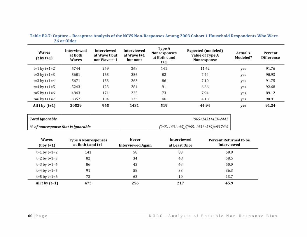
60 | P a g e N O R C — A n a l y s i s o f P o s s i b l e N o n ‐ R e s p o n s e B i a s
Table B2.7: Capture – Recapture Analysis of the NCVS NonResponses Among 2003 Cohort 1 Household Respondents Who Were
26 or Older
Waves
(t by t+1)
Interviewed at Both
Waves
Interviewed at Wave t but not t+1 Wave
Interviewed at Wave t+1 bu t t t no
Type A Nonresponses at Both t and
t+1
Expected (modeled) Value of Type A
Nonresponse
Actual > Modeled?
Percent Difference
t=1 by t+1=2 5744 249 268 141 11.62 yes 91.76 t=2 by t+1=3 5681 165 256 82 7.44 yes 90.93 t=3 by t+1=4 5671 153 263 86 7.10 yes 91.75 t=4 by t+1=5 5243 123 284 91 6.66 yes 92.68 t=5 by t+1=6 4843 171 225 73 7.94 yes 89.12 t=6 by t+1=7 3357 104 135 46 4.18 yes 90.91 All t by (t+1) 30539 965 1431 519 44.94 yes 91.34
Total ignorable (965+1431+45)=2441
% of nonresponse that is ignorable (965+1431+45)/(965+1431+519)=83.74%
Waves
(t by t+1)
t=1 by t+1=2
Type A Nonresponses at Bot nd t+1 h t a
141
Never
Interviewed Again
Interviewed
at Le Once ast
83
Percent Returned to be Interviewed
58.9 58 t=2 by t+1=3 82 34 48 58.5 t=3 by t+1=4 86 43 43 50.0 t=4 by t+1=5 91 58 33 36.3 t=5 by t+1=6 73 63 10 13.7 All t by (t+1) 473 256 217 45.9

61 |
P a g e N O R C — A n a l y s i s o f P o s s i b l e N o n ‐ R e s p o n s e B i a s
Appendix C
Table C.3. 1: Data Level, Analyses Performed and Data Used
Level Basic Analyses Data Used
All Sample Households Disposition by geographic detail Public Use Files: 2002, 2007
All Contacted Households Type A Nonresponse and response by geographic detail and Race
Public Use Files: 2002, 2007
Interviewed Households for Annual Analyses
Response to collection year by geographic, socio‐demographic and victimization responses
Public Use Files: 2002, 2007
Interviewed Individuals for Annual Analyses
Response to collection year by socio‐demographic and crime incidents
Public Use Files: 2002, 2007
Interviewed Cohort Households
1) nt
Wave Response to collection year bysocio‐demographic and crime incide
nicle s
2) Logistic Model predicting chroresponders
3) Factors reflecting differential nonresponse
Linked Household Public Use Files: 2003 ‐ 2006: Internal Created File 2002‐2005
Interviewed Cohort Individuals Wave Response to collection year by socio‐demographic and crime incidents
Linked Individual Public Use Files: 2003 – 2006
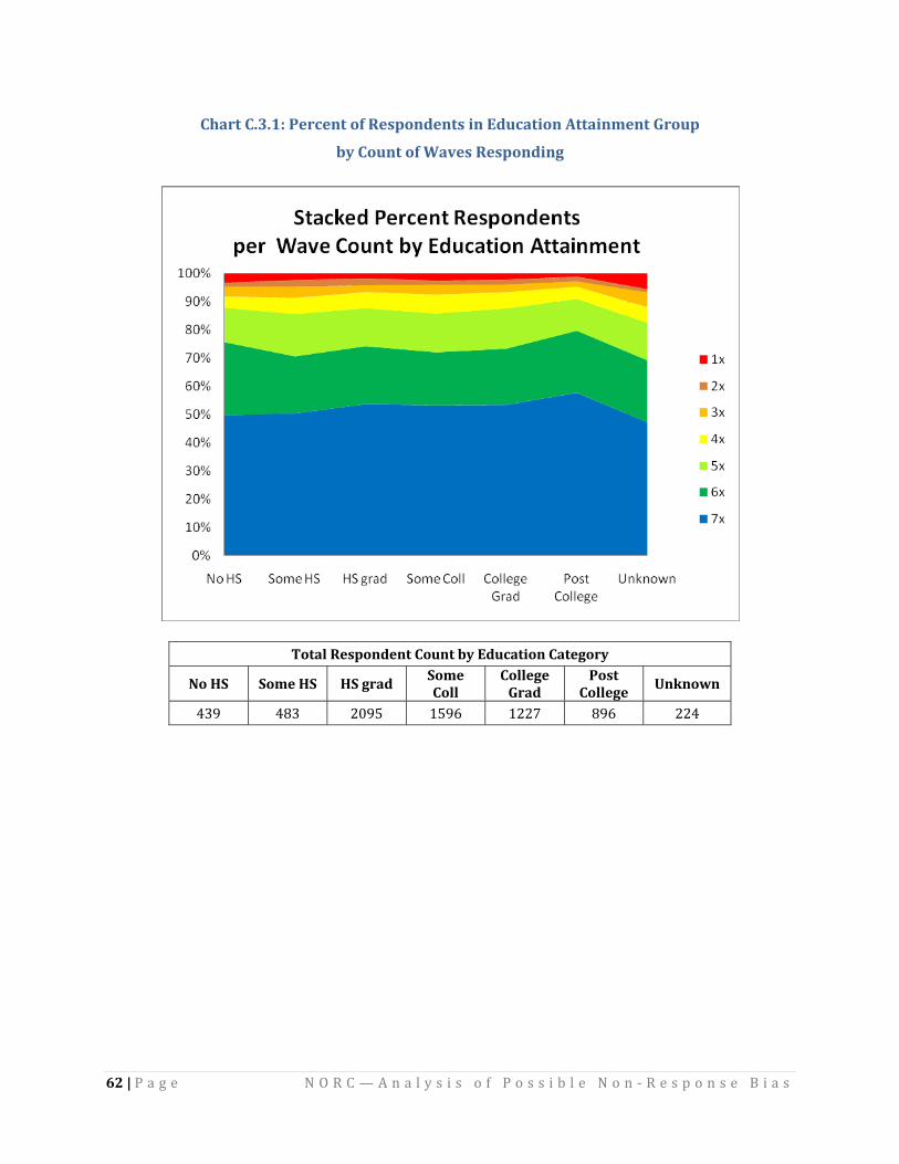
62 |
P a g e N O R C — A n a l y s i s o f P o s s i b l e N o n ‐ R e s p o n s e B i a s
Chart C.3.1: Percent of Respondents in Education Attainment Group
by Count of Waves Responding
Total Respondent Count by Education Category
N o HS So S me H H S gradSome Coll
College Grad
Post College
Un n know
439 483 2095 1596 1227 896 224

63 |
P a g e N O R C — A n a l y s i s o f P o s s i b l e N o n ‐ R e s p o n s e B i a s
Chart C.3.2: Percent of Respondents by Household Income Group
by Count of Waves Responding
Total Respondent Count by Household Income Category
m issing <=$ 0015,0 $15,000 <= $30,000
$30,000 <=$ 50,000
$50,000 <=$ 00 75,0
>$ 075,00
1942 848 1054 1129 880 1107

64 |
P a g e N O R C — A n a l y s i s o f P o s s i b l e N o n ‐ R e s p o n s e B i a s
Chart C.3.3: Percent of Respondents by Education Attainment Group
by Count of Waves Responding
Chart C.3.4: Percent of Respondents by Hispanic Origin by Count of Waves

65 |
P a g e N O R C — A n a l y s i s o f P o s s i b l e N o n ‐ R e s p o n s e B i a s
Chart C.3.5: Percent of Respondents by Race by Count of Waves

66 |
P a g e N O R C — A n a l y s i s o f P o s s i b l e N o n ‐ R e s p o n s e B i a s
Tables C.3.2 – C.3.4: Household Logistic Regression Results Modeling Response to 6 or more Waves of Survey
Tables C.3.2: Response Profile Response Profile
Response to 6 or More Waves
Frequency
1 5147 0 1813
Tables C.3.3: Results Table
E stimate S td Error Wald Chi
Sqr PR q > ChiS
Intercept ‐0.6873 0.1242 30.6106 <.0001 Age Bounded (20,50) 0.0244 0 .00265 84.7242 <.0001 Hispanic Origin 0.3618 0.0968 13.9637 0.0002 Married 0 .2291 0.0656 1 2.1943 0 .0005Post College 0.259 0 .0924 7.8659 0.005 Rank of HH Income 0.0429 0.017 6.3592 0 .0117Black*Incidence Reported ‐0.4826 0.2021 5.6998 0.017 Midwest 0.2367 0.0689 11.8113 0.0006 Homeowner 0.6351 0.0658 9 3.2682 < .0001Family Structure = Male w/others ‐0.2278 0.0811 7.8839 0.005
Tables C.3.2: Association of Predicted Probabilities and Observed Responses
% Concordant 66 S omers' D 0.328 % Discordant 33.2 Gamma 0.331 Pairs 9331511 c 0.664

67 |
P a g e N O R C — A n a l y s i s o f P o s s i b l e N o n ‐ R e s p o n s e B i a s
Tables C.3.5 – C.3.7: Household Logistic Regression Results Modeling Drop Outs (Responded to 3 or Less Waves of Survey)
Tables C.3.5: Response Profile Response Profile
Drop Out Frequency
1 4850 6475
Tables C.3.6: Results Table
E stimate S r td Erro W iald Ch
Sqr PR q > ChiS
Intercept ‐1.4041 0.1879 55.85 <.0001 Age Bounded (20,50) ‐ 0.0177 0 .00435 16.62 <.0001 Married ‐0.563 0.1082 27.09 <.0001 Rank of HH Income ‐0.0795 0.0295 7.25 0.0071 black*Incidence Reported 0.9018 0.2581 12.21 0.0005 Asian*Married 0.8144 0.2875 8.02 0.0046 Rural 0.4311 0 .1151 14.02 0.0002 South 0.2574 0.098 6.89 0.0086 Homeowner ‐0.4362 0.1118 15.22 <.0001
Tables C.3.7: Association of Predicted Probabilities and Observed Responses
% Concordant 65.3 S omers' D 0.323 % Discordant 33.2 Gamma 0.328 Pairs 3140375 c 0.662
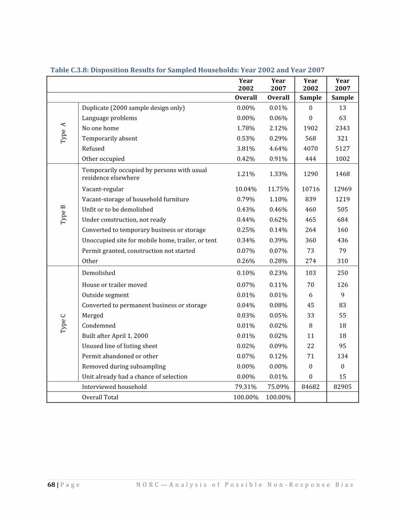
68 |
P a g e N O R C — A n a l y s i s o f P o s s i b l e N o n ‐ R e s p o n s e B i a s
Table C.3.8: Disposition Results for Sampled Households: Year 2002 and Year 2007
Year 2002
Year 2007
Year 2002
Year 2007
O verall O verall Sample Sample
Type A
Duplicate (2000 sample design only) 0.00% 0.01% 0 13 Language problems 0.00% 0.06% 0 63 No one home 1.78% 2.12% 1 902 2 343Temporarily absent 0.53% 0.29% 568 321 Refused 3.81% 4.64% 4 070 5127 Other occupied 0.42% 0.91% 444 1002
Type B
Temporarily occupied by persons with usual here residence elsew 1.21% 1.33% 1290 1468
Vacant‐regular 1 0.04% 1 1.75% 10716 12969 Vacant‐storage of household furniture 0.79% 1.10% 839 1 219Unfit or to be demolished 0.43% 0.46% 460 505 Under construction, not ready 0.44% 0.62% 465 684 Converted to temporary business or storage 0.25% 0.14% 264 160 Unoccupied site for mobile home, trailer, or tent 0.34% 0.39% 3 60 4 36Permit granted, construction not started 0.07% 0.07% 73 79 Other 0.26% 0.28% 274 310
Type C
Demolished 0.10% 0.23% 103 250
House or trailer moved 0.07% 0.11% 7 0 126 Outside segment 0.01% 0.01% 6 9 Converted to permanent business or storage 0.04% 0.08% 45 83 Merged 0.03% 0.05% 3 3 55 Condemned 0.01% 0.02% 8 18 Built after April 1, 2000 0.01% 0.02% 11 18 Unused line of listing sheet 0.02% 0.09% 22 95 Permit abandoned or other 0.07% 0.12% 7 1 134 Removed during subsampling 0.00% 0.00% 0 0 Unit already had a chance of selection 0.00% 0.01% 0 15
Interviewed household 79.31% 75.09% 84682 82905
Overall Total 100.00% 100.00%

69 |
P a g e N O R C — A n a l y s i s o f P o s s i b l e N o n ‐ R e s p o n s e B i a s
Chart C.3.6: Percent Responding Households by Education, 2002

70 |
P a g e N O R C — A n a l y s i s o f P o s s i b l e N o n ‐ R e s p o n s e B i a s
Table C.3.10: Logistic Regression: Year 2002 – Predicting Household NonResponse to One of the First Two Interviews. (Respondents = 29,381, Nonrespondents = 3,492)
Analysis of Maximum Likelihood Estimates
Parameter DF Estimate Standard Error
Wald C hiSquare Pr > ChiSq
Intercept 1 ‐1.3188 0.0890 2 19.5131 <.0001
Black 1 0.2448 0.0520 22.1376 <.0001
Age 1 ‐0.0165 0 .00211 60.9230 <.0001
Age > 60 1 ‐0.1808 0.0557 10.5345 0.0012
No High School 1 ‐0.3449 0.0912 1 4.3111 0.0002
Some College 1 ‐0.1261 0.0440 8.2266 0.0041
Unknown Household Income 1 0.3350 0.0395 71.8170 <.0001
Midwest 1 ‐0.2213 0.0453 23.8861 <.0001
Homeowner 1 ‐0.3518 0.0411 73.2911 <.0001
Family Structure: male with others 1 0.4922 0.0508 93.8105 <.0001
Family Structure: female with relatives 1 0.1696 0.0590 8.2728 0.0040
Family Structure: female with others 1 0.3724 0.0508 53.7224 <.0001
Not MSA 1 ‐0.1875 0.0576 10.5904 0.0011
Association of Pred Probabilities and Observed Responses icted
Percent Concordant 62.5 Somers' D 0.264
Percent Discordant 3 6.1 Gamma 0.268
Percent Tied 1.5 Taua 0.050
Pairs 102598452 c 0.632

71 |
P a g e N O R C — A n a l y s i s o f P o s s i b l e N o n ‐ R e s p o n s e B i a s
Table C.3.11: Logistic Regression – Year 2007 Predicting Household NonResponse to One of the First Two Interviews (Respondents = 28,378 Nonrespondents = 4,799)
Analysis of Maximum Likelihood Estimates
Parameter DF E stimateStandard Error
Wald Ch e iSquar Pr q > ChiS
Intercept 1 ‐0.2155 0.1027 4.3987 0.0360
Age 1 ‐0.0297 0.001 94 2 32.8924 <.0001
Young: Age 2535 1 ‐0.1188 0.0478 6.1910 0.0128
Hispanic Origin 1 ‐0.2638 0.0630 17.5553 <.0001
Married 1 ‐0.2248 0.0501 20.1593 <.0001
Widowed 1 ‐0.4027 0.0694 33.6292 <.0001
Never married 1 ‐0.1910 0.0517 13.6182 0.0002
Unknown Household Income 1 0.8210 0.0362 5 15.5699 <.0001
Household Income < $20,000 1 0.1478 0.0490 9.0893 0.0026
Number of Crime Incidents 1 0.1173 0.0301 15.2213 <.0001
Hispanic Origin, south & urban 1 0.4626 0.0965 23.0001 <.0001
Black, Midwest, & urban 1 0.3989 0.1034 14.8838 0.0001
Midwest 1 ‐0.2162 0.0426 25.7871 <.0001
Homeowner 1 ‐0.6664 0.0374 317.6972 <.0001
Family Structure:
Male with others 1 0.2840 0.0503 31.8971 <.0001
Family Structure: female with others 1 0.1657 0.0524 9.9810 0.0016
Association of Pred Probabilities and Observed Responses icted
Percent Concordant 68.7 Somers' D 0.386
Percent Discordant 3 0.2 Gamma 0.390
Percent Tied 1.1 Taua 0.095
Pairs 136186022 c 0.693

72 |
P a g e N O R C — A n a l y s i s o f P o s s i b l e N o n ‐ R e s p o n s e B i a s
Table C.3.12: Proportion of Individuals Reporting at Least One Crime Incidence, Using Data from the Public Use File, at the Person Level, from Quarters 3 and 4 of 2002 and Quarters 1 and 2 of 2003
Missi uted ng ImpPercent Difference:
(im d respondents espondents
pute)/r
Respo Only ndents
Overall 0.0438 ‐10 0.0486
Nonblack 0.0426 ‐ 12 0.0483 Black 0.0525 0 0.0526 ratio 1.2329 Female 0.0448 7 0.0420 Male 0.0429 ‐18 0.0523
0.9569 Hispanic Origin 0.0492 ‐2 0.0502 Non‐Hispanic 0.0431 ‐11 0.0485
0.8769 Age LT 25 0.0637 0 0.0637 Age 25‐35 0.0522 1 0 0.0474 Age 35‐45 0.0445 1 0.0442 Age 45‐55 0.0396 1 0.0391 Age 55‐65 0.0283 1 0.0281 Age GT 65 0.0145 ‐2 0.0148
Black ‐ Age LT 25 0.0678 ‐6 0.0725 Nonblack ‐ Age LT 25 0.0629 ‐1 0.0633
Black ‐ Age 25‐35 0.0598 2 1 0.0492 Nonblack ‐ Age 25‐35 0.0510 8 0.0472
Black ‐ Age 35‐45 0.0436 ‐2 0.0444 Nonblack ‐ Age 35‐45 0.0505 18 0.0428
Black ‐ Age 45‐55 0.0429 11 0.0384 Nonblack ‐ Age 45‐55 0.0392 ‐12 0.0444
Black ‐ Age 55‐65 0.0393 ‐ 11 0.0443 Nonblack ‐ Age 55‐65 0.0271 2 0.0265
Black ‐ Age GT 65 0.0204 ‐11 0.0230 Nonblack ‐ Age GT 65 0.0139 ‐1 0.0141

73 |
P a g e N O R C — A n a l y s i s o f P o s s i b l e N o n ‐ R e s p o n s e B i a s
Table C.3.13: Logistic Regression – Year 2002 Predicting Individual NonResponse to Wave 3 Given Response to Wave 2 (Respondents = 12,205 Nonrespondents = 2336)
Analysis of Maximum Likelihood Estimates
Parameter D F E stimateStandard Error
Wald Ch iSquare Pr q > ChiS
Intercept 1 ‐2.2967 0.0502 2 092.8849 <.0001
Age < 25 1 0.9020 0.0611 218.1104 <.0001
Age 25 to 35 1 0.8840 0.0644 188.1 504 <.0001
Age 35 to 45 1 0.3051 0.0686 19.77 07 <.0001
Black 1 0.1711 0.0670 6.5207 0.0107
High School Graduate 1 0.2737 0.0540 25.6782 <.0001
Some College 1 0.2753 0.0592 21.6153 <.0001
Crime Incidence for Age < 25
1 0.7326 0.1462 25.1125 <.0001
Association of Predicte bilities and Observed Responses d Proba
Percent Concordant 57.7 Somers' D 0.249
Percent Discordant 3 2.8 Gamma 0.275
Percent Tied 9.5 Taua 0.067
Pairs 28510880 c 0.625
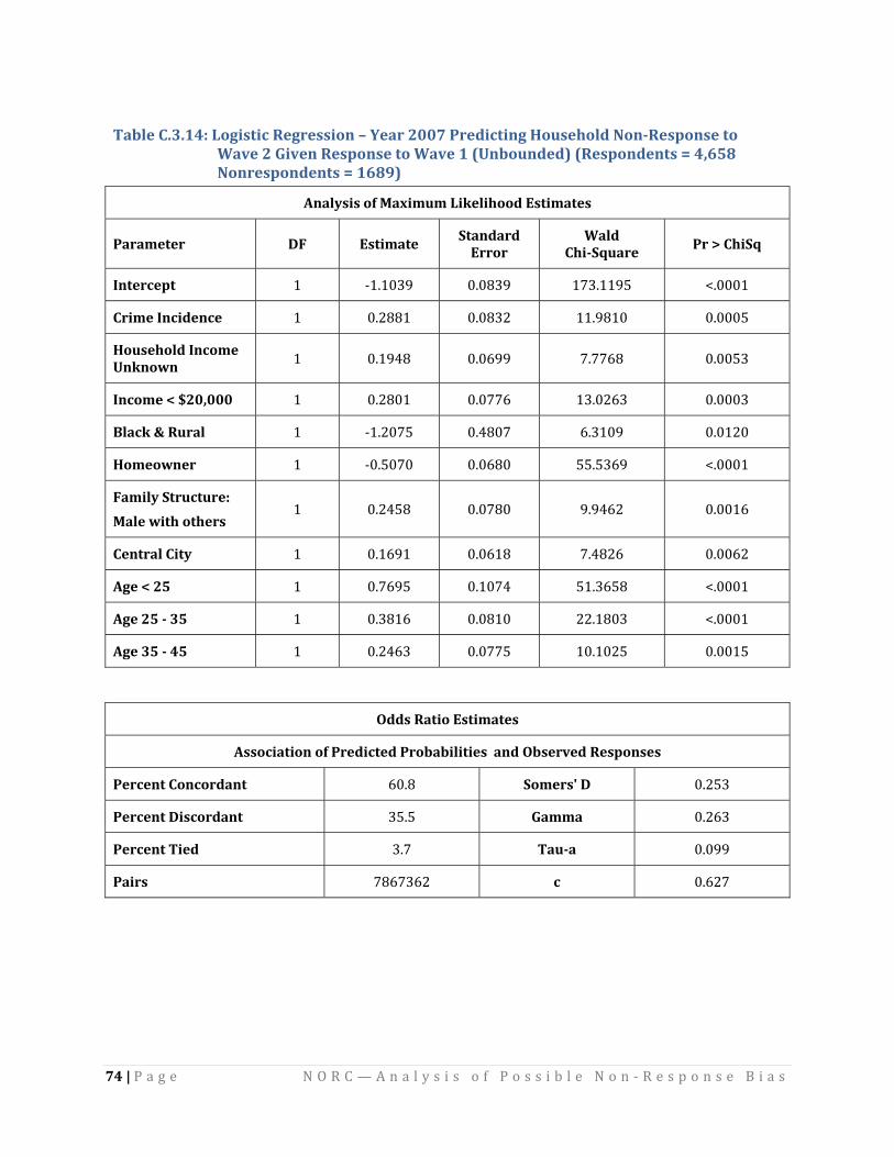
74 | P a g e N O R C — A n a l y s i s o f P o s s i b l e N o n ‐ R e s p o n s e B i a s
Table C.3.14: Logistic Regression – Year 2007 Predicting Household NonResponse to
Wave 2 Given Response to Wave 1 (Unbounded) (Respondents = 4,658 Nonrespondents = 1689)
Analysis of Maximum Likelihood Estimates
Parameter DF Estimate Standard Error
Wald C hiSquare Pr > ChiSq
Intercept 1 ‐1.1039 0.0839 173.1 195 <.0001
Crime Incidence 1 0.2881 0.0832 1 1.9810 0.0005
Household Income Unknown 1 0.1948 0.0699 7.7768 0.0053
Income < $20,000 1 0.2801 0.0776 1 3.0263 0.0003
Black & Rural 1 ‐1.2075 0.4807 6.3109 0.0120
Homeowner 1 ‐0.5070 0.0680 55.5369 <.0001
Family Structure:
Male with others 1 0.2458 0.0780 9.9462 0.0016
Central City 1 0.1691 0.0618 7.4826 0.0062
Age < 25 1 0.7695 0.1074 51.3658 <.0001
Age 25 35 1 0.3816 0.0810 22.1803 <.0001
Age 35 45 1 0.2463 0.0775 10.1025 0.0015
Odds Ratio Estimates
Association of Predicte babilities and Observed Responses d Pro
Percent Concordant 60.8 Somers' D 0.253
Percent Discordant 3 5.5 Gamma 0.263
Percent Tied 3.7 Taua 0.099
Pairs 7867362 c 0.627

75 |
P a g e N O R C — A n a l y s i s o f P o s s i b l e N o n ‐ R e s p o n s e B i a s
Appendix D
Table D.3.1a: Refusal and Crime Rate by Region, Place Size and Race, Year =2002, Northeast
Region Place Size Race Sample Size
Number Resp nts onde
Number Re lsfusa
Refusal R ate
Crime Rate
Northeast Not in a place Nonblack 5 271 4 860 4 11 8% 0.0533 Northeast Not in a place Black 151 133 18 1 2% 0.0827 Northeast Under 10,000 Nonblack 2599 2402 1 97 8% 0.0745 Northeast Under 10,000 Black 89 76 13 15% 0.1053 Northeast 10,000‐49,999 Nonblack 3 525 3 168 3 57 10% 0.0688 Northeast 10,000‐49,999 Black 284 249 35 12% 0.0522 Northeast 50,000‐99,999 Nonblack 1 423 1 277 1 46 10% 0.0744 Northeast 50,000‐99,999 Black 176 156 20 11% 0.1218 Northeast 100,000‐249,999 Nonblack 732 661 71 10% 0.1074 Northeast 100,000‐249,999 Black 213 184 29 14% 0.0924 Northeast 250,000‐499,999 Nonblack 229 192 37 16% 0.1198 Northeast 250,000‐499,999 Black 138 108 30 22% 0.1389 Northeast 500,000‐999,999 Nonblack 172 1 49 23 13% 0.0671 Northeast 500,000‐999,999 Black 60 44 16 2 7% 0.0909 Northeast 1,000,000‐2,499,999 Nonblack 341 324 17 5% 0.0957 Northeast 1,000,000‐2,499,999 Black 225 214 11 5% 0.0888 Northeast 2,500,000‐4,999,999 Nonblack 2 033 1 700 333 16% 0.0547 Northeast 2,500,000‐4,999,999 Black 727 586 141 19% 0.0546

76 |
P a g e N O R C — A n a l y s i s o f P o s s i b l e N o n ‐ R e s p o n s e B i a s
Table D.3.1b: Refusal and Crime Rate by Region, Place Size and Race, Year =2002, Midwest
Region Place Size Race Sample Size
Number Resp nts onde
Number Re ls fusa
Refusal R ate
Crime Rate
Midwest Not in a place Nonblack 4 980 4 731 2 49 5% 0.0668 Midwest Not in a place Black 156 137 19 1 2% 0.0876 Midwest Under 10,000 Nonblack 3 503 3 325 178 5% 0.0695 Midwest Under 10,000 Black 135 131 4 3% 0.1069 Midwest 10,000‐49,999 Nonblack 5 127 4 854 2 73 5% 0.0806 Midwest 10,000‐49,999 Black 345 326 19 6% 0.0706 Midwest 50,000‐99,999 Nonblack 1 798 1 710 88 5% 0.0906 Midwest 50,000‐99,999 Black 199 179 20 1 0% 0.0670 Midwest 100,000‐249,999 Nonblack 1 363 1 283 80 6% 0.1200 Midwest 100,000‐249,999 Black 201 188 13 6% 0.1223 Midwest 250,000‐499,999 Nonblack 758 703 55 7% 0.1238 Midwest 250,000‐499,999 Black 208 192 16 8% 0.1667 Midwest 500,000‐999,999 Nonblack 686 636 50 7% 0.1132 Midwest 500,000‐999,999 Black 332 3 07 2 5 8% 0.1140 Midwest 1,000,000‐2,499,999 Nonblack 59 55 4 7% 0.1636 Midwest 1,000,000‐2,499,999 Black 260 253 7 3% 0.1502 Midwest 2,500,000‐4,999,999 Nonblack 641 542 99 15% 0.1070 Midwest 2,500,000‐4,999,999 Black 326 277 49 15% 0.1516

77 |
P a g e N O R C — A n a l y s i s o f P o s s i b l e N o n ‐ R e s p o n s e B i a s
Table D.3.1c: Refusal and Crime Rate by Region, Place Size and Race, Year =2002, South
Region Place Size Race Sample Size
Number Respondents
Number Re ls fusa
Refusal R ate
Crime Rate
South Not in a place Nonblack 9913 9326 5 87 6% 0.0655 South Not in a place Black 1491 1400 91 6% 0.0543 South Under 10,000 Nonblack 3 657 3 457 2 00 5% 0.0793 South Under 10,000 Black 846 801 45 5% 0.0612 South 10,000‐49,999 Nonblack 5362 5 074 2 88 5% 0.0877 South 10,000‐49,999 Black 1006 949 57 6% 0.0790 South 50,000‐99,999 Nonblack 1 440 1 337 1 03 7% 0.1174 South 50,000‐99,999 Black 406 376 30 7% 0.0851 South 100,000‐249,999 Nonblack 2 144 1 998 1 46 7% 0.1091 South 100,000‐249,999 Black 633 588 45 7% 0.0986 South 250,000‐499,999 Nonblack 1 856 1 716 1 40 8% 0.1200 South 250,000‐499,999 Black 652 593 59 9% 0.0877 South 500,000‐999,999 Nonblack 831 750 81 10% 0.1053 South 500,000‐999,999 Black 545 492 53 10% 0.0915 South 1,000,000‐2,499,999 Nonblack 807 747 60 7% 0.1406 South 1,000,000‐2,499,999 Black 280 264 16 6% 0.1288
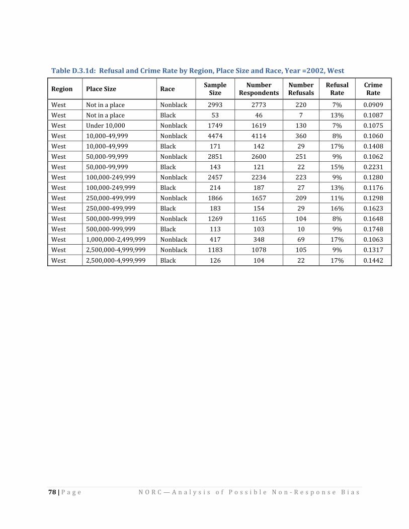
78 |
P a g e N O R C — A n a l y s i s o f P o s s i b l e N o n ‐ R e s p o n s e B i a s
Table D.3.1d: Refusal and Crime Rate by Region, Place Size and Race, Year =2002, West
Region Place Size Race Sample Size
Number Resp nts onde
Number Re ls fusa
Refusal R ate
Crime Rate
West Not in a place Nonblack 2993 2773 220 7% 0.0909 West Not in a place Black 53 46 7 1 3% 0.1087 West Under 10,000 Nonblack 1749 1619 130 7% 0.1075 West 10,000‐49,999 Nonblack 4 474 4 114 3 60 8% 0.1060 West 10,000‐49,999 Black 171 142 29 1 7% 0.1408 West 50,000‐99,999 Nonblack 2 851 2 600 2 51 9% 0.1062 West 50,000‐99,999 Black 143 121 22 1 5% 0.2231 West 100,000‐249,999 Nonblack 2 457 2 234 2 23 9% 0.1280 West 100,000‐249,999 Black 214 187 27 13% 0.1176 West 250,000‐499,999 Nonblack 1 866 1 657 2 09 11% 0.1298 West 250,000‐499,999 Black 183 154 29 1 6% 0.1623 West 500,000‐999,999 Nonblack 1 269 1 165 1 04 8% 0.1648 West 500,000‐999,999 Black 113 103 10 9% 0.1748 West 1,000,000‐2,499,999 Nonblack 417 348 69 1 7% 0.1063 West 2,500,000‐4,999,999 Nonblack 1 183 1 078 1 05 9% 0.1317 West 2,500,000‐4,999,999 Black 126 104 22 17% 0.1442

79 |
P a g e N O R C — A n a l y s i s o f P o s s i b l e N o n ‐ R e s p o n s e B i a s
Figure D.3.2: Refusal and Crime Rate by Region, Place Size and Race, Year =2007
[only groups with at least 50 households included in graph]

80 |
P a g e N O R C — A n a l y s i s o f P o s s i b l e N o n ‐ R e s p o n s e B i a s
Table D.3.2a: Refusal and Crime Rate by Region, Place Size and Race, Year =2002, Northeast
Region Place Size Race Sample Size
Number Resp nts onde
Number Re ls fusa
Refusal Rate
Crime Rate
Northeast Not in a place Nonblack 5 150 4 585 5 65 11% 0.0635 Northeast Not in a place Black 142 108 34 24% 0.1204 Northeast Under 10,000 Nonblack 2451 2223 2 28 9% 0.0625 Northeast Under 10,000 Black 101 86 15 15% 0.1163 Northeast 10,000‐49,999 Nonblack 3524 3045 4 79 14% 0.0631 Northeast 10,000‐49,999 Black 301 261 40 13% 0.1226 Northeast 50,000‐99,999 Nonblack 1212 1053 1 59 13% 0.0665 Northeast 50,000‐99,999 Black 110 90 20 18% 0.0889 Northeast 100,000‐249,999 Nonblack 587 516 71 12% 0.0736 Northeast 100,000‐249,999 Black 114 101 13 11% 0.0792 Northeast 250,000‐499,999 Nonblack 1 64 1 26 38 23% 0.0556 Northeast 250,000‐499,999 Black 98 83 15 15% 0.0723 Northeast 500,000‐999,999 Nonblack 1 40 1 00 40 29% 0.1300 Northeast 500,000‐999,999 Black 48 36 12 25% 0.1111 Northeast 1,000,000‐2,499,999 Nonblack 273 262 1 1 4% 0.1260 Northeast 1,000,000‐2,499,999 Black 194 190 4 2% 0.1053 Northeast 5,000,000 or more Nonblack 1 791 1 423 368 21% 0.0485 Northeast 5,000,000 or more Black 661 557 104 16% 0.0521

81 |
P a g e N O R C — A n a l y s i s o f P o s s i b l e N o n ‐ R e s p o n s e B i a s
Table D.3.2b: Refusal and Crime Rate by Region, Place Size and Race, Year =2002, Midwest
Region Place Size Race Sample Size
Number Resp nts onde
Number Re ls fusa
Refusal R ate
Crime Rate
Midwest Not in a place Nonblack 5 951 5620 331 6% 0.0653 Midwest Not in a place Black 105 78 27 2 6% 0.0513 Midwest Under 10,000 Nonblack 3613 3379 234 6% 0.0636 Midwest Under 10,000 Black 143 117 26 1 8% 0.0855 Midwest 10,000‐49,999 Nonblack 4849 4506 343 7% 0.0728 Midwest 10,000‐49,999 Black 448 392 56 1 3% 0.1173 Midwest 50,000‐99,999 Nonblack 2049 1891 158 8% 0.0989 Midwest 50,000‐99,999 Black 197 181 16 8% 0.0829 Midwest 100,000‐249,999 Nonblack 1284 1170 114 9% 0.0718 Midwest 100,000‐249,999 Black 188 178 10 5% 0.1236 Midwest 250,000‐499,999 Nonblack 564 497 67 12% 0.1368 Midwest 250,000‐499,999 Black 263 232 31 1 2% 0.0948 Midwest 500,000‐999,999 Nonblack 481 436 45 9% 0.0963 Midwest 500,000‐999,999 Black 407 364 43 11% 0.1264 Midwest 2,500,000‐4,999,999 Nonblack 565 446 119 21% 0.0852 Midwest 2,500,000‐4,999,999 Black 219 162 57 26% 0.1420

82 |
P a g e N O R C — A n a l y s i s o f P o s s i b l e N o n ‐ R e s p o n s e B i a s
Table D.3.2c: Refusal and Crime Rate by Region, Place Size and Race, Year =2002, South
Region Place Size Race Sample Size
Number Respondents
Number Re ls fusa
Refusal R ate
Crime Rate
South Not in a place Nonblack 1 0241 9471 770 8% 0.0624 South Not in a place Black 1404 1291 113 8% 0.0790 South Under 10,000 Nonblack 3 871 3 615 2 56 7% 0.0786 South Under 10,000 Black 780 725 55 7% 0.0634 South 10,000‐49,999 Nonblack 5316 4876 4 40 8% 0.0810 South 10,000‐49,999 Black 1133 1044 89 8% 0.0805 South 50,000‐99,999 Nonblack 2 203 2 033 1 70 8% 0.0969 South 50,000‐99,999 Black 484 461 23 5% 0.1106 South 100,000‐249,999 Nonblack 2 152 1 964 1 88 9% 0.0860 South 100,000‐249,999 Black 797 726 71 9% 0.0937 South 250,000‐499,999 Nonblack 1 136 1 053 83 7% 0.0959 South 250,000‐499,999 Black 270 256 14 5% 0.0977 South 500,000‐999,999 Nonblack 1 427 1 278 1 49 1 0% 0.1221 South 500,000‐999,999 Black 659 600 59 9% 0.1117 South 1,000,000‐2,499,999 Nonblack 1 058 905 1 53 14% 0.1492 South 1,000,000‐2,499,999 Black 274 226 48 18% 0.1593

83 |
P a g e N O R C — A n a l y s i s o f P o s s i b l e N o n ‐ R e s p o n s e B i a s
Table D.3.2d: Refusal and Crime Rate by Region, Place Size and Race, Year =2002, West
Region Place Size Race Sample Size
Number Respondents
Number Re ls fusa
Refusal Rate
Crime Rate
West Not in a place Nonblack 2342 2103 239 10% 0.0780 West Not in a place Black 39 31 8 2 1% 0.1935 West Under 10,000 Nonblack 2303 2086 217 9% 0.0820 West Under 10,000 Black 28 21 7 25% 0.0000 West 10,000‐49,999 Nonblack 4 148 3 704 444 11% 0.0940 West 10,000‐49,999 Black 160 135 25 16% 0.1111 West 50,000‐99,999 Nonblack 2 315 2 066 249 11% 0.1016 West 50,000‐99,999 Black 178 141 37 21% 0.0993 West 100,000‐249,999 Nonblack 3 489 3 091 398 11% 0.1081 West 100,000‐249,999 Black 269 231 38 14% 0.1212 West 250,000‐499,999 Nonblack 1 735 1 505 230 13% 0.1076 West 250,000‐499,999 Black 185 152 33 18% 0.1316 West 500,000‐999,999 Nonblack 1046 934 112 11% 0.1103 West 500,000‐999,999 Black 70 54 16 23% 0.0926 West 1,000,000‐2,499,999 Nonblack 775 691 8 4 1 1% 0.0999 West 1,000,000‐2,499,999 Black 43 42 1 2% 0.1905 West 2,500,000‐4,999,999 Nonblack 920 791 129 14% 0.0847 West 2,500,000‐4,999,999 Black 137 109 28 20% 0.0367

Figure D.3.3 – Refusal and Crime Rate by Region, MSA Status, Land Use and Race, Year =2002
[only groups with at least 50 households included in graph]
84 | P a g e N O R C — A n a l y s i s o f P o s s i b l e N o n ‐ R e s p o n s e B i a s

Table D.3.3a: Refusal and Crime Rate by Region, MSA Status, Land Use and Race, Year =2002, Northeast & Midwest
Region MSA Status Land Use Race Sample Size
Number Re nts sponde
Number Re ls fusa
Ref ate usal R Cr teime Ra
Northeast Central city Urban Nonblack 4451 3903 548 12% 0.0764 Northeast Central city Urban Black 1440 1211 229 16% 0.0801 Northeast MSA but not central city Urban Nonblack 7952 7213 739 9% 0.0641 Northeast MSA but not central city Urban Black 574 495 79 14% 0.0788 Northeast MSA but not central city Rural Nonblack 2556 2354 202 8% 0.0497 Northeast MSA but not central city Rural Black 42 37 5 12% 0.0541 Northeast Not MSA Urban Nonblack 323 297 26 8% 0.0976 Northeast Not MSA Urban Black 1 1 0 0% 0.0000 Northeast Not MSA Rural Nonblack 1043 966 77 7% 0.0756 Northeast Not MSA Rural Black 6 6 0 0% 0.0000 Midwest Central city Urban Nonblack 4742 4401 341 7% 0.1122 Midwest Central city Urban Black 1471 1350 121 8% 0.1304 Midwest MSA but not central city Urban Nonblack 7785 7319 466 6% 0.0761 Midwest MSA but not central city Urban Black 596 551 45 8% 0.0835 Midwest MSA but not central city Rural Nonblack 2750 2610 140 5% 0.0640 Midwest MSA but not central city Rural Black 33 30 3 9% 0.1000 Midwest Not MSA Urban Nonblack 1409 1375 34 2% 0.0931 Midwest Not MSA Urban Black 53 50 3 6% 0.0800 Midwest Not MSA Rural Nonblack 2229 2134 95 4% 0.0595 Midwest Not MSA Rural Black 9 9 0 0% 0.2222
85 | P a g e N O R C — A n a l y s i s o f P o s s i b l e N o n ‐ R e s p o n s e B i a s

86 | P a g e N O R C — A n a l y s i s o f P o s s i b l e N o n ‐ R e s p o n s e B i a s
Table D.3.3b: Refusal and Crime Rate by Region, MSA Status, Land Use and Race, Year =2002, South and West
Region MSA Status Land Use Race Sample Size
Number Re nts sponde
Number Re ls fusa
Refusal Rate Crime Rate
South Central city Urban Nonblack 6742 6252 490 7% 0.1190 South Central city Urban Black 2519 2336 183 7% 0.0967 South MSA but not central city Urban Nonblack 10160 9515 645 6% 0.0846 South MSA but not central city Urban Black 1748 1588 160 9% 0.0781 South MSA but not central city Rural Nonblack 4919 4622 297 6% 0.0699 South MSA but not central city Rural Black 395 367 28 7% 0.0545 South Not MSA Urban Nonblack 1118 1065 53 5% 0.0610 South Not MSA Urban Black 454 442 12 3% 0.0498 South Not MSA Rural Nonblack 3071 2951 120 4% 0.0535 South Not MSA Rural Black 743 730 13 2% 0.0397 West Central city Urban Nonblack 7418 6699 719 10% 0.1373 West Central city Urban Black 576 498 78 14% 0.1687 West MSA but not central city Urban Nonblack 8915 8156 759 9% 0.1038 West MSA but not central city Urban Black 482 402 80 17% 0.1343 West MSA but not central city Rural Nonblack 1168 1072 96 8% 0.1035 West MSA but not central city Rural Black 8 7 1 13% 0.0000 West Not MSA Urban Nonblack 828 773 55 7% 0.1061 West Not MSA Urban Black 4 4 0 0% 0.5000 West Not MSA Rural Nonblack 930 888 42 5% 0.0563 West Not MSA Rural Black 3 3 0 0% 0.3333

Figure D.3.4: Refusal and Crime Rate by Region, MSA Status, Land Use and Race, Year =2007
[only groups with at least 50 households included in graph]
87 | P a g e N O R C — A n a l y s i s o f P o s s i b l e N o n ‐ R e s p o n s e B i a s

Table D.3.4a: Refusal and Crime Rate by Region, MSA Status, Land Use and Race, Year =2007, Northeast & Midwest
Region MSA Status Land Use Race Sample Size
Number Re nts sponde
Number Re ls fusa
Ref ate usal R Cr te ime Ra
Northeast Central city Urban Nonblack 3944 3289 655 17% 0.0696 Northeast Central city Urban Black 1202 1049 153 13% 0.0753 Northeast MSA but not central city Urban Nonblack 8161 7182 979 12% 0.0596 Northeast MSA but not central city Urban Black 541 446 95 18% 0.1054 Northeast MSA but not central city Rural Nonblack 1704 1509 195 11% 0.0663 Northeast MSA but not central city Rural Black 8 3 5 63% 0.0000 Northeast Not MSA Urban Nonblack 525 481 44 8% 0.0873 Northeast Not MSA Urban Black 11 9 2 18% 0.2222 Northeast Not MSA Rural Nonblack 958 872 86 9% 0.0608 Northeast Not MSA Rural Black 7 5 2 29% 0.4000 Midwest Central city Urban Nonblack 4541 4082 459 10% 0.0980 Midwest Central city Urban Black 1271 1112 159 13% 0.1124 Midwest MSA but not central city Urban Nonblack 7174 6605 569 8% 0.0636 Midwest MSA but not central city Urban Black 542 464 78 14% 0.1056 Midwest MSA but not central city Rural Nonblack 2241 2113 128 6% 0.0487 Midwest MSA but not central city Rural Black 13 7 6 46% 0.1429 Midwest Not MSA Urban Nonblack 1857 1763 94 5% 0.0930 Midwest Not MSA Urban Black 116 108 8 7% 0.1111 Midwest Not MSA Rural Nonblack 3543 3382 161 5% 0.0716 Midwest Not MSA Rural Black 28 13 15 54% 0.0769
88 | P a g e N O R C — A n a l y s i s o f P o s s i b l e N o n ‐ R e s p o n s e B i a s
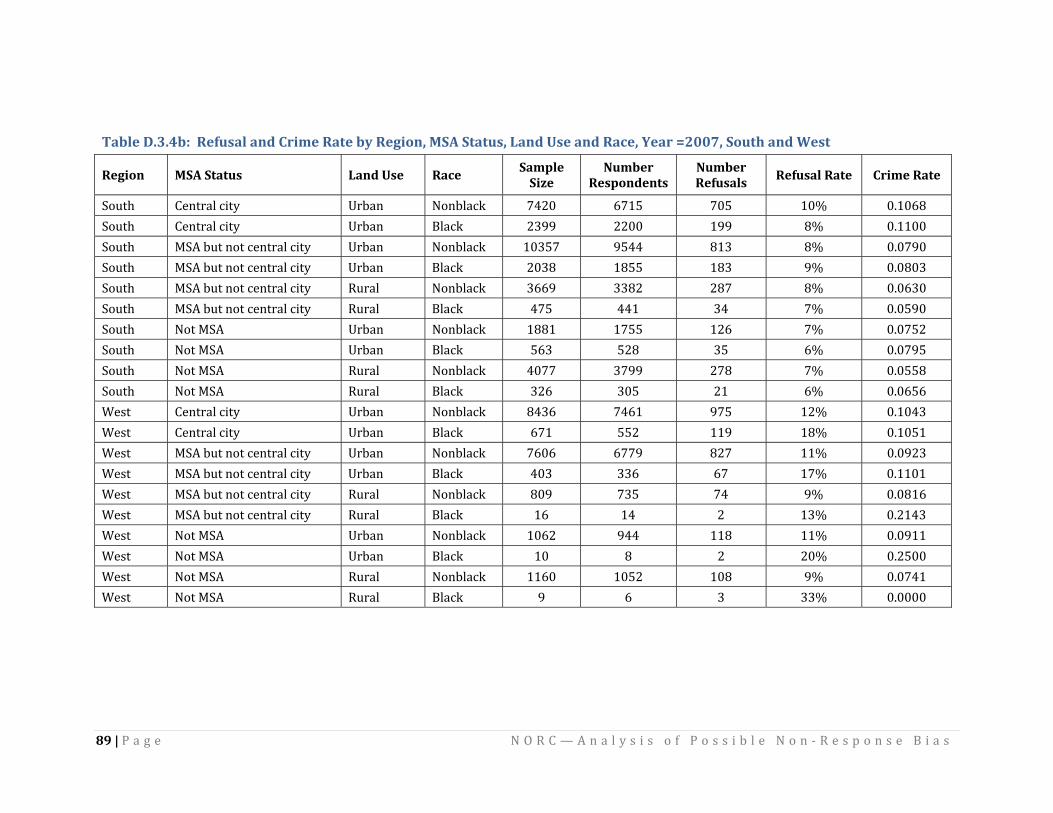
89 | P a g e N O R C — A n a l y s i s o f P o s s i b l e N o n ‐ R e s p o n s e B i a s
Table D.3.4b: Refusal and Crime Rate by Region, MSA Status, Land Use and Race, Year =2007, South and West
Region MSA Status Land Use Race Sample Size
Number Re nts sponde
Number Re ls fusa Ref ate usal R Cr te ime Ra
South Central city Urban Nonblack 7420 6715 705 10% 0.1068 South Central city Urban Black 2399 2200 199 8% 0.1100 South MSA but not central city Urban Nonblack 10357 9544 813 8% 0.0790 South MSA but not central city Urban Black 2038 1855 183 9% 0.0803 South MSA but not central city Rural Nonblack 3669 3382 287 8% 0.0630 South MSA but not central city Rural Black 475 441 34 7% 0.0590 South Not MSA Urban Nonblack 1881 1755 126 7% 0.0752 South Not MSA Urban Black 563 528 35 6% 0.0795 South Not MSA Rural Nonblack 4077 3799 278 7% 0.0558 South Not MSA Rural Black 326 305 21 6% 0.0656 West Central city Urban Nonblack 8436 7461 975 12% 0.1043 West Central city Urban Black 671 552 119 18% 0.1051 West MSA but not central city Urban Nonblack 7606 6779 827 11% 0.0923 West MSA but not central city Urban Black 403 336 67 17% 0.1101 West MSA but not central city Rural Nonblack 809 735 74 9% 0.0816 West MSA but not central city Rural Black 16 14 2 13% 0.2143 West Not MSA Urban Nonblack 1062 944 118 11% 0.0911 West Not MSA Urban Black 10 8 2 20% 0.2500 West Not MSA Rural Nonblack 1160 1052 108 9% 0.0741 West Not MSA Rural Black 9 6 3 33% 0.0000

Appendix E
Appendix E4.1: Crime Victimization Rates by Census Divisions, in Year 2006
Crime Victimization
ALL Rates by Census Division
Count All
Divisions
New England (1)
Middle Atlantic (2)
East North Central (3)
West North Central (4)
South Atlantic (5)
East South Central (6)
West South Central (7)
Mountain (8)
Pacific (9)
Assault 3308527 1.338% 1.185% 1.099% 1.247% 0.918% 0.966% 0.905% 2.055% 1.682% 1.876% Burglary 2433133 0.984% 0.520% 0.783% 1.177% 0.787% 0.709% 0.856% 1.484% 1.252% 1.124% Motor Vehicle Theft 801504 0.324% 0.052% 0.142% 0.386% 0.250% 0.256% 0.204% 0.321% 0.590% 0.549% Purse Snatching 148124 0.060% 0.097% 0.069% 0.042% 0.002% 0.035% 0.009% 0.083% 0.091% 0.107% Rape 185893 0.075% 0.028% 0.048% 0.058% 0.039% 0.070% 0.101% 0.133% 0.120% 0.085% Robbery 512377 0.207% 0.190% 0.180% 0.202% 0.151% 0.182% 0.053% 0.279% 0.245% 0.296% Theft 10502638 4.248% 3.555% 3.016% 3.891% 3.248% 3.236% 2.525% 6.269% 5.832% 6.224% All Crime 17892196 7.237% 5.626% 5.338% 7.002% 5.395% 5.454% 4.652% 10.625% 9.812% 10.262% Total Persons 247244481 11575994 33630342 39861140 18144654 46877523 15433425 25649354 17413243 38658806 Source: NCVS, 2006
90 | P a g e N O R C — A n a l y s i s o f P o s s i b l e N o n ‐ R e s p o n s e B i a s

Appendix E4.2: Arrests Reported in the Uniform Crime Reports (UCR) in Counties where the National Crime Victimization Survey (NCVS) Data Were Collected, in Year 2006
Crime Arrest All
Census Division
New England (1)
Middle Atlantic (2)
East North Central (3)
West North Central (4)
South Atlantic (5)
East South Central (6)
West South Central (7)
Mountain (8)
Pacific (9)
Aggravated Assaults 285453 14742 53632 25691 14297 31547 9957 31591 12783 91213Burglaries 178766 6818 30041 18177 8227 23467 9589 20984 9493 51970Larcenies 664528 28140 124780 86123 48684 81174 35728 95032 53070 111797Murders 9359 226 2085 1146 396 1259 597 1158 524 1968Motor Vehicle Thefts 95238 2012 16675 15021 5348 8158 2942 7920 7991 29171Rapes 13826 735 2968 1602 843 1384 610 2182 846 2656Robberies 94235 3736 24871 11833 3835 11462 4178 8535 4354 21431Combined except Murder 1332046 56183 252967 158447 81234 157192 63004 166244 88537 308238All Combined 1341405 56409 255052 159593 81630 158451 63601 167402 89061 310206Total County Population Where Agencies Report Arrests 197426932 10135367 32027981 29064515 9149697 34997248 7709295 22548902 12275104 39518823
Source: UCR, 2006
91 | P a g e N O R C — A n a l y s i s o f P o s s i b l e N o n ‐ R e s p o n s e B i a s

Appendix E4.3: Crime Victimization Rates by Census Divisions, in Year 2005
Crime Victimization
ALL Rates by Census Division
Count All
Divisions
New England (1)
Middle Atlantic (2)
East North Central (3)
West North Central (4)
South Atlantic (5)
East South Central (6)
West South Central (7)
Mountain (8)
Pacific (9)
Assault 3211231 1.313% 1.124% 1.404% 1.387% 0.707% 0.967% 0.579% 1.699% 1.820% 1.748% Burglary 2413114 0.987% 0.894% 0.603% 1.079% 0.783% 0.848% 0.575% 1.716% 1.476% 1.015% Motor Vehicle Theft 861993 0.353% 0.278% 0.238% 0.336% 0.225% 0.249% 0.158% 0.536% 0.582% 0.530% Purse Snatching 165341 0.068% 0.018% 0.101% 0.059% 0.053% 0.052% 0.016% 0.160% 0.031% 0.065% Rape 140607 0.058% 0.018% 0.080% 0.026% 0.084% 0.034% 0.024% 0.115% 0.101% 0.058% Robbery 544742 0.223% 0.061% 0.345% 0.294% 0.151% 0.217% 0.086% 0.238% 0.293% 0.174% Theft 10390651 4.250% 3.260% 3.450% 3.948% 2.874% 3.511% 2.077% 6.424% 6.738% 5.496% All Crime 17727679 7.250% 5.653% 6.223% 7.129% 4.877% 5.877% 3.515% 10.889% 11.040% 9.086% Total Persons 244504326 12917601 31587129 37522638 19583401 46137495 17626940 24590162 13091564 41447396 Source: NCVS, 2005
92 | P a g e N O R C — A n a l y s i s o f P o s s i b l e N o n ‐ R e s p o n s e B i a s

93 | P a g e N O R C — A n a l y s i s o f P o s s i b l e N o n ‐ R e s p o n s e B i a s
Appendix E4.4: Arrests Reported in the Uniform Crime Reports (UCR) in Counties where the National Crime Victimization Survey (NCVS) Data Were Collected, in Year 2005
Crime Arrest All
Census Division
New England (1)
Middle Atlantic (2)
East North Central (3)
West North Central (4)
South Atlantic (5)
East South Central (6)
West South Central (7)
Mountain (8)
Pacific (9)
Aggravated Assaults 277205 11835 51281 27498 13699 33970 11379 24299 11458 91786Burglaries 170587 6307 28133 17460 7330 24985 8199 17560 10788 49825Larcenies 686897 25504 131468 83408 47457 94373 33244 94308 60892 116243Murders 9155 196 1852 1281 377 1347 570 1118 463 1951Motor Vehicle Thefts 103310 2255 17914 16795 5985 9444 3148 7684 8314 31771Rapes 14272 635 3034 2276 1060 1662 519 1861 746 2479Robberies 86434 3111 23740 11017 3932 11549 3834 6988 3494 18769Combined except Murder 1338705 49647 255570 158454 79463 175983 60323 152700 95692 310873All Combined 1347860 49843 257422 159735 79840 177330 60893 153818 96155 312824Total County Population Where Agencies Report Arrests 191800897 10061367 32989936 27386916 8831912 35592394 6803765 20327739 11335722 38471146
Source: UCR, 2005

94 |
P a g e N O R C — A n a l y s i s o f P o s s i b l e N o n ‐ R e s p o n s e B i a s
Appendix E4.5: List of Counties Where the UCR Crime Counts Were Zero
Stat IPSe F C ode
stcnty U_TOT_CRIME U_CPOPARST N_Tot_Crime N_Total_Persons
12 12001 0 227627 32149 680570 12 12005 0 6 39119 7 3363 2 19383512 12007 0 28592 2643 84798 12 12011 0 7 112336 5 21811 6 63143012 12013 0 13514 1266 224326 12 12019 0 657963 28948 560490 12 12025 0 2375298 226252 3873287 12 12031 0 3 336768 3 20539 2 99155712 12041 0 47355 4622 764319 12 12045 0 14211 1519 283774 12 12053 0 441405 6064 263190 12 12057 0 4 447774 3 97454 3695300 12 12061 0 500985 30002 3843254 12 12071 0 2 067339 2 18434 4198683 12 12075 0 111860 11803 1 42031712 12083 0 308560 32425 841905 12 12086 0 4 833033 2 06209 4 32765812 12089 0 255081 4055 135314 12 12091 0 546541 22105 1600441 12 12095 0 4 002656 1 05496 2 73923512 12097 0 864096 27350 869680 12 12099 0 5016717 316203 4368781 12 12101 0 1628891 172185 1297853 12 12103 0 3783580 382554 2892441 12 12105 0 2 117942 1 85779 2 67332312 12109 0 604735 11950 249382 12 12115 0 1446896 2 56446 4206164 12 12117 0 1 592307 5 6428 1 41060517 17007 0 50637 7867 136840 17 17023 0 51070 5483 1 10910317 17027 0 1 33360 2468 152920 17 17045 0 58184 6237 1 52116017 17063 0 46051 0 31053 17 17083 0 88108 4524 76068 17 17093 0 257714 10687 421130 17 17097 0 710486 65361 618147 17 17111 0 1220427 106435 959169

Appendix E4.5: List of Counties Where the UCR Crime Counts Were Zero
P a g e N O R C — A n a l y s i s o f P o s s i b l e N o n ‐ R e s p o n s e B i a s
Stat IPSe F C ode
stcnty U_TOT_CRIME U_CPOPARST N_Tot_Crime N_Total_Persons
17 17115 0 1 10759 21696 7 7706417 17117 0 49769 11658 71664 17 17119 0 1 068433 1 16289 1 00025917 17133 0 121077 7829 124619 17 17163 0 1 027004 1 40007 882645 17 17179 0 517644 1 5427 847377 17 17203 0 1 47407 2522 214663 27 27101 0 8911 79 217353 51 51780 0 0 1418 285360
95 |
Appendix E4.6: List of Counties Where the NCVS Crime Counts Were Zero
State IPS F Co e d
stcnt y U_TOT_CRIME U_CPOPARST N_Tot_Crime N_Total_Persons
1 1007 85 21662 0 21858 8 8039 20 2 3219 0 24285 8 8047 68 5025 0 13157 8 8093 29 17269 0 0 13 13015 619 92095 0 84969 13 13083 205 48449 0 35402 13 13227 245 29705 0 6597 17 17063 0 46051 0 31053 18 18013 14 15254 0 17316 19 19085 20 15968 0 30999 19 19129 53 1 5365 0 27260 21 21077 49 8198 0 9371 21 21211 740 1 08950 0 68035 22 22037 185 19737 0 9651 22 22047 301 30697 0 32487 22 22075 1 34 2 7483 0 0 22 22091 83 9724 0 10734 26 26037 8 4 6 8387 0 124808 27 27077 4 4451 0 1 5571828 28093 276 35530 0 23021 28 28137 1 34 26452 0 17129 29 29049 86 25421 0 13510 29 29177 491 96439 0 112691

96 |
P a g e N O R C — A n a l y s i s o f P o s s i b l e N o n ‐ R e s p o n s e B i a s
Appendix E4.6: List of Counties Where the NCVS Crime Counts Were Zero
Stat IPSe F C ode
stcnty U_TO IME T_CR U_CPOPARST N_Tot_Crime N_Total_Persons
29 29219 1 93 28939 0 24272 31 31025 18 25874 0 22980 32 32023 3 78 41830 0 55396 35 35057 83 17739 0 18570 36 36041 52 15826 0 1 6798537 37053 1 39 23573 0 7490 40 40117 49 17004 0 0 42 42025 815 1 81474 0 1 2845047 47047 148 34896 0 17436 47 47057 2 89 65091 0 43104 47 47173 51 19319 0 14568 48 48019 53 20554 0 20324 48 48055 128 36502 0 15982 48 48221 187 49288 0 44933 48 48259 137 28482 0 11254 48 48325 195 43880 0 33614 48 48473 705 1 38583 0 31630 49 49043 186 36142 0 2797 51 51033 112 25818 0 12288 51 51075 1 77 74641 0 86437 51 51093 89 33750 0 11502 51 51099 67 20843 0 14680 51 51101 55 14879 0 15541 51 51109 50 30307 0 2523 51 51145 28 2 6863 0 32010 51 51181 37 7083 0 11340 51 51187 93 35910 0 9206 51 51630 260 20939 0 5476 51 51683 394 1 13456 0 22192 51 51830 2 12 35192 0 36913 55 55047 97 19330 0 1 1813355 55093 216 41853 0 21941

97 |
P a g e N O R C — A n a l y s i s o f P o s s i b l e N o n ‐ R e s p o n s e B i a s
Appendix F
Figure F4.1: Total Counts of Crime Incidents – NCVS by UCR, in 2003 – 2006, By Region

98 |
P a g e N O R C — A n a l y s i s o f P o s s i b l e N o n ‐ R e s p o n s e B i a s
Figure F4.2: Logarithms of Total Counts of Crime ncidents–NCVS I
by UCR, in 2003–2006, By Region

99 |
P a g e N O R C — A n a l y s i s o f P o s s i b l e N o n ‐ R e s p o n s e B i a s
Figure F4.3: Total Counts of Crime Incidents – NCVS by UCR, in 2003 – 2006, by Region
Excluding counties where total victimization incident count =0 and arrest count =0

100 |
P a g e N O R C — A n a l y s i s o f P o s s i b l e N o n ‐ R e s p o n s e B i a s
Figure F4.4: Countylevel Burglary Crime Victimization Estimates
in NCVS by Burglary Offense Arrests in UCR, 2006

101 |
P a g e N O R C — A n a l y s i s o f P o s s i b l e N o n ‐ R e s p o n s e B i a s
Appendix F4.1: Crime Victimization Incidents at Selected Areas – Unweighted
Table F4.1.1: Crime Victimization by YEAR
Bronx, NY YEAR
Total 2003 2004 2005 2006
Rape/ sault Sexual As 0 0 2 0 2 Robbery 1 1 4 3 9 Assault 8 5 1 1 9 3 3
Purse Snatc ket Picking hing/Poc 0 1 0 0 1
Burglary 3 5 3 1 1 2Motor Vehicle Theft 1 0 0 1 2
Theft 19 9 14 11 53 Total 32 21 34 25 112
Frequency Missing = 2938
Table F4.1.2: Crime Victimization by YEAR
Cook County
YEAR Total
2003 2004 2005 2006 Rape/ sault Sexual As 2 0 1 0 3
Robbery 16 4 11 1 32 Assault 2 0 3 1 2 6 1 7 94
Purse Snatc ket Picking hing/Poc 9 8 3 1 21
Burglary 36 49 2 3 3 8 1 46Motor Vehicle Theft 15 12 9 8 44
Theft 135 118 103 91 447 Total 233 222 176 156 787
Frequency Missing = 13630

102 |
P a g e N O R C — A n a l y s i s o f P o s s i b l e N o n ‐ R e s p o n s e B i a s
Table F4.1.3: Crime Victimization by YEAR
Kings (Brooklyn), NY)
YEAR Total
2003 2004 2005 2006 Rape/ sault Sexual As 0 0 0 0 0
Robbery 2 7 3 2 14 Assault 9 6 8 9 3 2
Purse Snatc ket Picking hing/Poc 2 0 3 0 5
Burglary 1 2 6 2 4 2 4Motor Vehicle Theft 2 2 1 1 6
Theft 25 24 21 21 91 Total 52 45 38 37 172
Frequency Missing = 6152
Table F4.1.4: Crime Victimization by YEAR
Manhattan
YEAR Total
2003 2004 2005 2006 Rape/ sault Sexual As 0 0 0 0 0
Robbery 2 2 0 0 4 Assault 1 1 7 5 4 2 7
Purse Snatc ket Picking hing/Poc 0 1 0 0 1
Burglary 2 1 3 4 1 0Motor Vehicle Theft 1 0 0 1 2
Theft 32 25 18 14 89 Total 48 36 26 23 133
Frequency Missing = 3215

103 |
P a g e N O R C — A n a l y s i s o f P o s s i b l e N o n ‐ R e s p o n s e B i a s
Table 4.1.5: Crime Victimization by YEAR
Other
YEAR T otal
2003 2004 2005 2006 Rape/ sault Sexual As 84 73 61 94 312
Robbery 200 175 170 219 764 Assault 1686 1571 1319 1720 6 296
Purse Snatc ket Picking hing/Poc 70 75 68 59 272
Burglary 1 493 1 481 1 324 1 477 5775 Motor Vehicle Theft 451 462 386 363 1662
Theft 6308 6227 5309 6054 23898 Total 10292 10064 8637 9986 38979
Frequency Missing = 698734
Table F4.1.6: Crime Victimization by YEAR
Queens, NY
YEAR Total
2003 2004 2005 2006 Rape/ sault Sexual As 0 0 0 0 0
Robbery 2 1 1 0 4 Assault 5 4 8 6 2 3
Purse Snatc ket Picking hing/Poc 1 2 0 1 4
Burglary 2 0 5 5 1 2Motor Vehicle Theft 2 1 3 0 6
Theft 28 15 19 21 83 Total 40 23 36 33 132
Frequency Missing = 5122

104 |
P a g e N O R C — A n a l y s i s o f P o s s i b l e N o n ‐ R e s p o n s e B i a s
Table F4.1.7: Crime Victimization by YEAR
Richmond (Staten Island), NY
YEAR Total
2003 2004 2005 2006 Rape/ sault Sexual As 0 0 0 0 0
Robbery 0 0 0 0 0 Assault 0 5 1 0 6
Purse Snatc ket Picking hing/Poc 0 0 1 0 1
Burglary 0 0 0 0 0 Motor Vehicle Theft 1 0 0 0 1
Theft 6 3 9 3 21 Total 7 8 11 3 29
Frequency Missing = 1290

105 |
P a g e N O R C — A n a l y s i s o f P o s s i b l e N o n ‐ R e s p o n s e B i a s
Appendix F4.2: Crime Victimization Incidents at Selected Areas Weighted
Table F4.2.1: Crime Victimization by YEAR Bronx, NY
YEAR Total
2003 2004 2005 2006 Rape/ sault Sexual As 0 0 11222 0 11222
Robbery 3525.3 3964 16988 7444.2 31921 Assault 30720 12467 34407 28506 106100
Purse Snatc ket Picking hing/Poc 0 2009.2 0 0 2009.2 Burglary 7013.2 10088 7246.1 3176.6 27524
Motor Vehicle Theft 2455.7 0 0 2953.6 5409.3 Theft 44469 20990 37510 32604 135573 Total 88183.2 49518.3 107373 74684.7 319759
Table F4.2.2: Crime Victimization by YEAR
Cook County
YEAR Total
2003 2004 2005 2006 Rape/ sault Sexual As 4741.7 0 2293.6 0 7035.3
Robbery 43937 11369 41296 3887.6 100489 Assault 53439 80658 83334 62013 27944 4
Purse Snatc ket Picking hing/Poc 23123 21021 10195 2514.5 56854
Burglary 78417 1 05845 62576 1 09027 355865 Motor Vehicle Theft 34186 28637 26864 23395 113082
Theft 310313 252023 256998 255492 1074826 Total 548157 499553 483557 456328 1987595

106 |
P a g e N O R C — A n a l y s i s o f P o s s i b l e N o n ‐ R e s p o n s e B i a s
Table F4.2.3: Crime Victimizatio by YEAR n
Kings (Brooklyn), NY) YEAR
Total 2003 2004 2005 2006
Rape/ sault Sexual As 0 0 0 0 0 Robbery 6626.1 19072 9269.3 11135 46103 Assault 25948 15127 28418 27758 97251
Purse Snatc ket Picking hing/Poc 7302.4 0 8386.1 0 15689
Burglary 32397 13283 4984.5 11821 62485 Motor Vehicle Theft 5263.9 4826.6 2779.8 2379.8 15250
Theft 58896 49130 54896 57826 220747 Total 136433 101439 108734 110920 457525
Table F4.2.4: Crime Victimization by YEAR
Manhattan YEAR
Total 2003 2004 2005 2006 Rape/ sault Sexual As 0 0 0 0 0
Robbery 5514.6 5894.7 0 0 11409 Assault 37628 17266 13651 10696 79240
Purse Snatc ket Picking hing/Poc 0 2514.6 0 0 2514.6
Burglary 4835.8 2235.3 7675.2 11560 26306 Motor Vehicle Theft 2226.6 0 0 2557.7 4784.3
Theft 73614 52602 46664 38686 211566 Total 123819 80512.6 67990.2 63498.6 335820

107 |
P a g e N O R C — A n a l y s i s o f P o s s i b l e N o n ‐ R e s p o n s e B i a s
Table F4.2.5: Crime Victimization by YEAR
Other
YEAR Total
2003 2004 2005 2006 Rape/ sault Sexual As 243632 197019 187509 322314 950473
Robbery 546659 461567 536933 714888 2260046 Assault 4 430054 42672 94 4 180266 55604 62 1 .84E+07
Purse Snatc ket Picking hing/Poc 185342 221487 247161 198477 852466
Burglary 3582029 3478690 3647753 4130200 1.48E+07 Motor Vehicle Theft 1019022 1040342 1039877 1061089 4160330
Theft 1.46E+07 1.46E+07 1.41E+07 1.67E+07 6.00E+07 Total 2.46E+07 2.42E+07 2.39E+07 2.87E+07 1.02E+08
Frequency Missing = 396010.16212
Table F4.2.6: Crime Victim zation by YEAR i
Queens, NY YEAR
Total 2003 2004 2005 2006
Rape/ sault Sexual As 0 0 0 0 0 Robbery 5565.5 2213.6 2576 0 10355 Assault 14143 1 0620 24858 22763 72384
Purse Snatc ket Picking hing/Poc 2178.9 5958 0 3386.8 11524 Burglary 4481.2 0 9333.3 13282 27097
Motor Vehicle Theft 4398.7 1908.5 8006.4 0 14314 Theft 67595 33809 46238 60097 207739 Total 98362.7 54509.4 91011.3 99528.4 343412
Frequency Missing = 4654.9130483

108 | P a g e N O R C — A n a l y s i s o f P o s s i b l e N o n ‐ R e s p o n s e B i a s
Table F4.2.7: Crime Victimization by YEAR
Richmond (Staten Island), NY
YEAR Total
2003 2004 2005 2006 Rape/ sault Sexual As 0 0 0 0 0
Robbery 0 0 0 0 0 Assault 0 12009 1281.6 0 13291
Purse Snatc ket Picking hing/Poc 0 0 2368.2 0 2368.2
Burglary 0 0 0 0 0 Motor Vehicle Theft 2589.4 0 0 0 2589.4
Theft 13437 6623.5 21230 8262.5 49553 Total 16026.4 18632.7 24879.5 8262.48 67801.1

Appendix F4.3: UCR Arrest Rates for Selected Areas, 2003 (per 1,000)
Area Murder Rape Robbery Aggressive Assault
Burglary Larceny Motor Vehicle Theft
Cook County, IL 0.087909 0.11231 0.54179 1.04038 0.61927 3.21165 1.56485 Bronx, NY 0.078519 0.12915 1.12127 1.85803 1.07064 4.76175 1.29225 Kings (Brooklyn), NY 0.078641 0.12865 1.12114 1.85714 1.06952 4.76201 1.29173 New York (Manhattan), NY 0.081683 0.12928 1.13648 1.89028 1.07924 4.80192 1.29599 Queens, NY 0.078535 0.12896 1.1218 1.86833 1.07182 4.78394 1.29226 Richmond (Staten Island), NY 0.078282 0.1283 1.13074 1.8592 1.07203 4.77305 1.29166
Appendix F4.4: UCR Arrest Rates for Selected Areas, 2004 (per 1,000)
Area Murder Rape Robbery Aggressive Assault Burglary Larceny
Motor Vehicle Theft
Cook County, IL 0.080988 0.10493 0.54503 1.0506 0.55887 3.0076 1.38578 Bronx, NY 0.074887 0.13289 1.13431 2.13867 1.13211 5.24794 1.40449 Kings (Brooklyn), NY 0.07529 0.13336 1.13656 2.13856 1.13215 5.24748 1.40488 New York (Manhattan), NY 0.075454 0.13393 1.14816 2.17685 1.15005 5.38365 1.40533 Queens, NY 0.075113 0.13334 1.13736 2.15382 1.13469 5.26456 1.40536 Richmond (Staten Island), NY 0.075669 0.13404 1.14801 2.14036 1.1372 5.25795 1.40529
109 | P a g e N O R C — A n a l y s i s o f P o s s i b l e N o n ‐ R e s p o n s e B i a s

Appendix F4.5: UCR Arrest Rates for Selected Areas, 2005 (per 1,000)
Area Murder Rape Robbery Aggressive Assault
Burglary Larceny Motor Vehicle Theft
Cook County, IL 0.072 0.10209 0.57924 1.06917 0.5281 2.80048 1.31808 Bronx, NY 0.10458 0.13573 1.21267 2.54031 1.27646 5.94989 1.30316 Kings (Brooklyn), NY 0.10438 0.13621 1.20738 2.5401 1.2763 5.94866 1.30289 New York (Manhattan), NY 0.10522 0.13862 1.223 2.56887 1.28475 6.04506 1.30428 Queens, NY 0.1045 0.1359 1.20918 2.54753 1.27735 5.97952 1.30337 Richmond (Staten Island), NY 0.1044 0.13636 1.21874 2.54401 1.27627 5.95094 1.30183
Appendix F4.6: UCR Arrest Rates for Selected Areas, 2006 (per 1,000)
Area Murder Rape Robbery Aggressive Assault
Burglary Larceny Motor Vehicle Theft
Cook County, IL 0.05846 0 0.60328 0.94216 0.52275 2.51796 1.0902 Bronx, NY 0.14074 0.14442 1.29612 2.80076 1.43022 5.70173 1.17748 Kings (Brooklyn), NY 0.14098 0.14418 1.29762 2.79949 1.42978 5.69871 1.17747 New York (Manhattan), NY 0.14099 0.14537 1.30897 2.84165 1.44996 5.7848 1.17739 Queens, NY 0.141 0.14412 1.29709 2.80656 1.43005 5.73003 1.18063 Richmond (Staten Island), NY 0.14138 0.14349 1.30616 2.80644 1.43065 5.69939 1.17744
110 | P a g e N O R C — A n a l y s i s o f P o s s i b l e N o n ‐ R e s p o n s e B i a s

Appendix F4.7: UCR Arrest Counts for Selected Areas, 2003
Area Murder Rape Robbery Aggressive A t ssaul Burglary Larceny
Motor Vehicle Theft
Cook County, IL 472 603 2909 5586 3325 17244 8402 Bronx, NY 107 176 1528 2532 1459 6489 1761 Kings (Brooklyn), NY 195 319 2780 4605 2652 11808 3203 New York (Manhattan), NY 127 201 1767 2939 1678 7466 2015 Queens, NY 176 289 2514 4187 2402 10721 2896 Richmond (Staten Island), NY 36 59 520 855 493 2195 594
Appendix F4.8: UCR Arrest Counts for Selected Areas, 2004
Area Murder Rape Robbery Aggressive A t ssaul
Burglary Larceny Motor Vehicle
Theft
Cook County, IL 433 561 2914 5617 2988 16080 7409 Bronx, NY 102 181 1545 2913 1542 7148 1913 Kings (Brooklyn), NY 188 333 2838 5340 2827 13103 3508 New York (Manhattan), NY 120 213 1826 3462 1829 8562 2235 Queens, NY 169 300 2559 4846 2553 11845 3162 Richmond (Staten Island), NY 35 62 531 990 526 2432 650
111 | P a g e N O R C — A n a l y s i s o f P o s s i b l e N o n ‐ R e s p o n s e B i a s

112 | P a g e N O R C — A n a l y s i s o f P o s s i b l e N o n ‐ R e s p o n s e B i a s
Appendix F4.9: UCR Arrest Counts for Selected Areas, 2005
Area Murder Rape Robbery Aggressive A t ssaul Burglary Larceny
Motor Vehicle Theft
Cook County, IL 383 543 3081 5687 2809 14896 7011 Bronx, NY 141 183 1635 3425 1721 8022 1757 Kings (Brooklyn), NY 259 338 2996 6303 3167 14761 3233 New York (Manhattan), NY 167 220 1941 4077 2039 9594 2070 Queens, NY 233 303 2696 5680 2848 13332 2906 Richmond (Staten Island), NY 49 64 572 1194 599 2793 611
Appendix F4.10: UCR Arrest Counts for Selected Areas, 2006
Area Murder Rape Robbery Aggressive A t ssaul Burglary Larceny
Motor Vehicle Theft
Cook County, IL 310 0 3199 4996 2772 13352 5781 Bronx, NY 191 196 1759 3801 1941 7738 1598 Kings (Brooklyn), NY 352 360 3240 6990 3570 14229 2940 New York (Manhattan), NY 225 232 2089 4535 2314 9232 1879 Queens, NY 316 323 2907 6290 3205 12842 2646 Richmond (Staten Island), NY 67 68 619 1330 678 2701 558

113 |
P a g e N O R C — A n a l y s i s o f P o s s i b l e N o n ‐ R e s p o n s e B i a s
Appendix G
ORC at the University of Chicago deas for the NCVS July 24, 2009 NI
Introduction
It is important to establish valid measures of crime, and it is also important to be able to observe changes in trends and patterns of crime. So naturally as lessons are learned from the experience of implementation and as new data collection methods and technologies are developed there have been and will continue to be recommendations to modify or redesign the NCVS to improve the quality of the data and data collection. However, for a program like this to be able to continue to contribute to policy and practice, ny modification or redesign needs to be cognizant of and attentive to impacts on trends nd treaa nd analysis from changes in design or methodology.
Based on extensive study and review by a consortium of experts and a report issued by the NAS, in 1992 the NCS was redesigned and became the NCVS. In 2008 the National Research Council of the NAS issued a report with new recommendations for a redesign of the NCVS. Naturally any such redesign is a long term process. As part of the longer term process BJS has been supporting methodological studies of the NCVS. Currently NORC is conducting two such studies: The Analysis of Possible NonResponse Bias in the National rime Victimization Survey (2008‐BJ‐CX‐K062) and An Examination of a Twelve Month eferenCR ce Period in the National Crime Victimization Survey (2008‐BJ‐CX‐K071).
At a meeting between the NORC team working on the non‐response bias study and the BJS staff working on the project, the question was raised about what could be done over the next 12 to 18 months that could immediately be implemented for the NCVS without a break in the current series. On July 23 a meeting was held at NORC including members of the teams working on the two NCVS methodological studies. The meeting was attended by Chet Bowie, Fritz Scheuren, Norman Bradburn, Zhiwei Zhang, James Carr, Lisa Lee, and Henry Brownstein. We discussed this question and our response follows.
Ideas for Implementation over the Coming Months
1: Paradata Constructions and Related Issues
a. Interviewer Information
ID: Work with the census bureau staff to ensure the analytic utility of the interviewer IDs and make immediate suggestions on how the interview IDs should be assigned, organized, stored during the survey cycles.

Demographic information: work with the Census Bureau DSD to formulate an operational plan to get the data; assess the data; and make recommendations on data coding and storing and database management.
Interviewer experience information: work with the Census Bureau to figure out the reliability and the validity of this measure and how the existing coding can be transformed into useful information such as experience in NCVS and experience in all surveys overall, and make suggestions how it may be coded in the future.
Information unavailable but potentially useful for consideration in future paradata collection: interviewers’ attitudes and confidence (“can convince almost anyone to respond”); interviewers’ education, occupational aspiration; use of cultural knowledge and local knowledge of the sample neighborhood; way of adapting to the NORC at the University of Chicago 2 Ideas for the NCVS July 24, 2009 situation at the doorstep; behaviors during the interviewer‐respondent interactions such as any intentional or unintentional departure by interviewers from the designed guidelines or instructions, observed respondents’ burden during the face‐to‐face interviews (is the respondent in a hurry to do something else?)
b. Frame Information
Current NCVS internal files contain some geographic information which were originally used for sample design such as PSU, county, and tract identifiers. A number of census tract level characteristics such as median age, median housing value, percent Hispanic, etc. were available in the existing NCVS internal files. These variables are very helpful for the study of the possible nonresponse bias and other victimization‐related researches but not all pertinent and influential variables that may affect the survey processes are included. One example of such variables is the “percentage of residents who moved in the past five years” which may influence the local pattern of the mobility and the percentage of movers in the NCVS. It is recommended to make a systematic effort to add variables by using the geographic identifiers. Practically, it is relatively convenient to do so because the analysis will be conducted at the Census Bureau and almost all of the variables to be added will come from the Census Bureau’s database and many of hich are publically available. This merging effort can be made smoother because f th able staff on the site. wo
e knowledge
Immediate: Assess the level of geographic units and prepare a list of socio‐
phic variables from the Census and merge them into the existing demogra
Lon
P a g e s p o n s e B i a s N O R C — A n a l y s i s o f P o s s i b l e N o n ‐ R e
NCVS internal files. g‐term:
facilitating and Assess the utility of the American Community Survey in improving the survey process. Merge the 2010 NCVS with the 2010 decennial Census.
114 |

P a g e N O R C — A n a l y s i s o f P o s s i b l e N o n ‐ R e s p o n s e B i a s
c. Cleaning the Survey History Record Information for Better Use
The Census Bureau has internal paradata association with the NCVS. These include (1) the Call‐history Data for CATI (i.e., for NCVS till June 2007); and (2) Audit Trail Data for CAPI which is currently used in the NCVS in July 2007 and onward. These data are probably extremely under‐utilized. The data were also not designed special for the formal paradata analytic. We recommend the follo
wing steps:
these data.
Assess and document fully the availability and coverage of
Assess the variables codings and the extent of the recodes
Perform recodes so that the data can be used as paradata to support
methodological studies of NCVS
Perform special analyses and recommend further analyses using these data.
Recommend how the future paradata in this area should be recorded and how the data should be collected and managed.
d. Contact Information
Other than Call‐history and Audit Trail Data, further information on the detailed ways of approaching and contacting the households and respondents are lacking. We recommend NORC at the University of Chicago 3 Ideas for the NCVS July 24, 009 collaborating with the Census staff to develop a list of interesting nformation that future paradata collections may use. 2i
2: Longitudinal NCVS Constructions and Related Analyses
The purpose of this effort would be to build upon what has been done by NORC and o convert NCVS Cross‐sectional Files into Longitudinal Files for the full 2003‐2009 period, hereby increasing the analytic utility of the surveys. tt
a. Immediate
Handle the limitations and contingencies such as movers.
Revise a previous data structure plan to cover the major contingencies (cases not matched, movers) and document the method and process of how the
longitudinal files are created
Conduct disclosure analysis to assess the feasibility of making the longitudinal cohort files as (i) PUF and (ii) as internal files for other staff to use and make recommendations for NJS to review.
115 |

116 |
P a g e N O R C — A n a l y s i s o f P o s s i b l e N o n ‐ R e s p o n s e B i a s
b. Shortterm
Apply the updated program to create the 2007 July‐Dec ember NCVS Cohort
Longitudinal file.
Collaborate with the Census Bureau in the file creation process and have the linkage variables double checked for each year to ensure quality control which will be necessary due to survey redesign or possible internal program
modifications and changes.
Create codebooks for the longitudinal files
Revise the program to make them as macro engines for multiple year NCVS processing and can be readily applied to any cohorts after the 2007 July‐December.
c. Related Analyses
Mak
e the followings comparisons:
• Compare the 2003 Jan‐June Cohort to 2003 July‐Dec Cohort Dec cohort to 2007 July‐Dec Cohort • Compare the 2003 July‐
On the following domains:
• Type A N
•
onresponses • onresponses Type Z n
• Crimes
• Movers Unbounded wave vs. all other waves
• ictimizations >2 in the three years in the repeated victimizations (i.e., # of v
• survey) Spatial distributions of the above
• • HLM model in the causal relationship
Latent class analysis of the status changes • NORC at the University of Chicago 4 Ideas for the NCVS July 24, 2009
117 | P a g e N O R C — A n a l y s i s o f P o s s i b l e N o n ‐ R e s p o n s e B i a s
3: Addressing Bias and Variance Reduction
a. Immediate Implementation
Routine housekeeping could be conducted to be able to successfully match waves over time in order to do any of the other ideas recommended.
Earlier interviews could be used to longitudinally impute (not reweight) data for
later NCVS wave nonresponse.
UCR data could be used, after light editing and longitudinal imputation, for ratio estimation of the NCVS.
b. Implementation Following Some Research
The screener could be further examined to increase interviewer compliance with BJS goals for the survey.
The NCVS paradata system could be redesigned to aim it simultaneously at continued successful survey departmental success, while also instrumenting it more fully for inference.
Processing could be sped up so analysis comes more closely, almost simultaneously, with data collection.
4: Bounding Procedures
As part of the NCVS 12‐month reference period contract, NORC examined the percentage of crime incidents reported for each month of the 6‐month reference period. The data showed that for the first few months of the reference period, the percentage of crimes reported drops as time between the interview and the incident increases. However, there is a slight increase in the percentage of crimes reported for the final two months of the reference period. This pattern suggests that telescoping is occurring. That is, some incidents that occurred outside the reference period are being reported as having occurred within the reference period.
To address problems of telescoping, many panel surveys employ bounding
procedures. The interviewer typically reminds the respondent of the information he/she reported in the prior round of the survey before conducting the current interview. However, in the NCVS, respondents are not reminded of incidents that were reported in prior interviews. Rather, the interviewer compares reports from the current and prior rounds and, if the interviewer feels there may be a duplicate report, s/he must ask the respondent questions to determine whether the incidents are duplicates. This procedure elies on the interviewer’s judgment on whether to ask the respondent about a possible uplicate report. rd

118 |
P a g e N O R C — A n a l y s i s o f P o s s i b l e N o n ‐ R e s p o n s e B i a s
The current procedures for bounding interviews in the NCVS could be revised. A procedure that involves the respondent in de‐duplicating reports may be more effective in limiting forward telescoping. NORC at the University of Chicago 5 Ideas for the NCVS July 24, 2009.

119 |
P a g e N O R C — A n a l y s i s o f P o s s i b l e N o n ‐ R e s p o n s e B i a s
5: Examining the Organization of Crime Event Information
Relatively little is known about how people store and organize information about crime events in memory. One way of studying this issue is through respondents’ verbal descriptions of the crimes they have experienced. These verbal protocols could be analyzed ith a focus on the types of event information that are spontaneously reported, and the rder awo nd organization of the crime event information.
The NCVS screener provides an opportunity to collect verbal protocols on crime events. For each crime elicited by a screener question, the respondent is asked to describe what happened. Although respondents might typically provide only a brief description of the incident, selected respondents could be asked to describe their crime experience in reater detail. This information may be useful in deciding what kinds of retrieval cues are ost effective and help inform future modifications to the screener.
gm 6 : Q esu tions about Design Elements Suggesting Possible Adjustments
a. A move to a 12‐month reference period will have implications for the survey beyond the question of incident reporting. With a longer reference period, telescoping will be more important. At present we understand very little about how the adjustment for using the first (unbounded) interview was arrived at or how it will have to be adjusted with a 12‐month reference period. Also, we have not been able to get a clear idea about how much information the interviewer has to use in deciding whether an incident reported in the current period has been reported in the last period. Apparently the determination as to whether it is a new or old incident is made by the interviewer at the end of the interview rather than by directly asking the respondent. The wording of the question also poses a problem because reporting incidents that occurred in the last 12‐months is different than reporting “since the last interview.” Not all respondents are interviewed at the same report in the fixed reporting period. We know from our analysis that there are patterns of reporting influenced by how far from the calendar date of the reporting period the interview is actually taking place. This problem will be greater when the reference period is 12‐months. A 12‐month reporting period will have implications for other aspects of the survey such as series crimes. The number of crimes in a specified period to qualify as a series crime will have to be adjusted. What is the proper number?
b. With a 12‐month reference period, more incidents will be reported thus triggering
more incident reports and increasing the burden on the respondent. It may reduce the willingness to cooperate in later rounds of the survey. One way to reduce the burden is to subsample the frequent crimes and get incident reports on only a sample of them. Research should be done on how to do this. What crimes incidents should be subsampled? What should the sampling rate be? Can one use the UCR to supplement the data on the types of crimes that are subsampled?
120 | P a g e N O R C — A n a l y s i s o f P o s s i b l e N o n ‐ R e s p o n s e B i a s
c. There is little research on the incident forms. Is all of the information there necessary? Is it necessary for all incidents? Reducing the detail or number of incident forms for NORC at the University of Chicago 6 Ideas for the NCVS July 24, 2009 respondents would reduce the respondent burden and should lead to better cooperation and better reporting of incidents.
d. The NCVS is one of the major sources of data on the cost of crime, at least of direct costs to victims. With a longer reference period, costs that were not reported with a 6‐month reference period because they fell outside the reporting period may now be reported. Some research is needed to know how to disentangle greater reported costs due to the increased number of incidents reported from those due to the longer period during which costs for a particular crime, e.g. prolonged health care expenses.
Conclusion
We thank you for this opportunity to present our ideas to you. The ideas presented above are suggestions and do not all necessarily rise to the level of recommendations. They are firmly rooted in a long history of involvement with the NCVS and ongoing interest and work in the methodological and operational aspects of the survey. But they were conceived as ideas for this particular purpose within a 24 hour period. So if BJS is interested, any or all of these are things we could develop further for or with BJS.
The redesign of NCS in the 1980s was lead by Al Biderman with a scientific advisory
group that was constituted to set the research addenda. Different groups such as NORC, SRC at Michigan, and individual scholars in different universities, worked with them to conduct a number of studies and experiments covering all aspects of the survey from sampling to questionnaire to reporting. The result was a coordinated comprehensive set of recommendations for the redesign. If BJS is planning such a coordinated approach to the current redesign NORC would be honored to be able to participate in that effort and to contribute in any way we can.