Report Number 11/71

Nonuniqueness in a minimal model for cell motility

by

L.S. Gallimore, J.P. Whiteley, S.L. Waters, J.R. King, J.M. Oliver

Oxford Centre for Collaborative Applied Mathematics

Mathematical Institute

24 - 29 St Giles’

Oxford

OX1 3LB

England

Mathematical Medicine and BiologyPage 1 of 31doi:10.1093/imammb/dqnxxx

Non–uniqueness in a minimal model for cell motility

L.S. GALLIMORE 1, J.P. WHITELEY2, S.L. WATERS3, J.R. KING4, J.M. OLIVER3

1. OCCAM, Mathematical Institute, University of Oxford,24-29 St. Giles’, Oxford, OX1 3LB, UK.

2. Department of Computer Science, University of Oxford,Wolfson Building, Parks Road, Oxford, OX1 3QD, UK

3. OCIAM, Mathematical Institute, University of Oxford,24-29 St. Giles’, Oxford, OX1 3LB, UK

4. School of Mathematical Sciences, University of Nottingham,University Park, Nottingham, NG7 2RD, UK

[Received on 23rd November 2011]

Two–phase flow models have been used previously to model cellmotility, however these have rapidlybecome very complicated, including many physical processes, and are opaque. Here we demonstrate thateven the simplest one–dimensional, two–phase, poroviscous, reactive flow model displays a number ofbehaviours relevant to cell crawling. We present stabilityanalyses that show that an asymmetric pertur-bation is required to cause a spatially uniform, stationarystrip of cytoplasm to move, which is relevantto cell polarization. Our numerical simulations identify qualitatively distinct families of travelling–wavesolution that co–exist at certain parameter values. Withineach family, the crawling speed of the striphas a bell–shaped dependence on the adhesion strength. The model captures the experimentally observedbehaviour that cells crawl quickest at intermediate adhesion strengths, when the substrate is neither toosticky nor too slippy.

Keywords: Cell crawling, cell adhesion, two–phase, reactive, poroviscous.

1. Introduction

The ability of cells to crawl through their surroundings is crucial to many biological processes, includ-ing wound healing, immunity and embryonic development (Bray, 2001). The interplay of mechanicalforces and biochemical control mechanisms, coupled with thefundamental nature of cell motility, hascaught the attention of many experimentalists and mathematical modellers alike. Yet despite consider-able efforts, how cells achieve motility is still only partially understood and consensus remains elusive(Mogilner, 2009).

1.1 Biological description of cell motility

Experimental observations of cell crawling have revealed key features common to different cell types.Cells form protrusions at their front which adhere to the substrate, the bulk of the cell is pulled forwardsand adhesions at the rear of the cell weaken and detach (Bray,2001; Mogilner, 2009). The degree towhich these steps occur simultaneously or sequentially andthe shape of the protrusion can vary consid-erably with cell type and environment (Bray, 2001). Examples of protrusion shapes include finger-likepseudopodia, “bulbous” lobopodia, flat sheet–like lamellipodia and small “hair–like” filopodia (Bray,2001).

It is widely accepted that a cell’s actin network is the main generator of protrusive force. Actin

c© The author 2008. Published by Oxford University Press on behalf of the Institute of Mathematics and its Applications. All rights reserved.

2 of 31 L.S. GALLIMORE et.al.

monomers polymerize into filaments that form the actin network. Filament ends are chemically distinct,denoted barbed and pointed, and have different polymerization rates. It has been shownin vitro thatat intermediate monomer concentrations, actin filaments grow and shrink at their barbed and pointedends respectively, a phenomenon termed treadmilling (Bray, 2001). A considerable step forward in theunderstanding of cell motility was provided by quantitative observations of actin dynamicsin vivo, fromfluorescent speckle microscopy (Waterman-Storeret al., 1998). This technique provided evidence ofstrong polymerization of the actin network at the leading edge and flow of the actin network backwards,away from the leading edge in the lamellipodium of a locomoting cell (Schaubet al., 2007; Vallottonetal., 2004, 2005).

The actin network is highly regulatedin vivo and we refer the interested reader to Pollard & Borisy(2003) for a clear description of the mechanisms and molecules involved, with the cautionary note thatrecent evidence is calling into question whether actin filaments branch in lamellipodia as was previ-ously thought (Small, 2010, 2011; Higgs, 2011; Insall, 2011). Svitkinaet al. (1997) presented imagesof steadily locomoting keratocytes that show the density ofthe actin network to be highest at the lead-ing edge of the cell and to decrease across the lamellapodia until the density peaks again where thelamellipodia join the cell body. The density of the actin network is much lower in the cell body. Thetransition between the near symmetric, ring–like actin distributions in a stationary cell and the polariseddistribution in a travelling cell can be triggered mechanically in fragments of keratocyte lamellipodia(Verkhovskyet al., 1999). Another mathematically interesting phenomenon attributed to actin networkdynamics is “ruffling”, where actin–containing folds in thecell membrane form periodically at the lead-ing edge of the cell and travel backwards over the lamellipodium (Hinzet al., 1999).

Having discussed protrusion and organisation of the actin network, we turn our attention to howthe cell anchors onto the substrate and generates the force required to haul its rear forwards. The actinnetwork is able to contract due to myosins, small motor proteins that use energy in the form of ATP toslide actin filaments past each other (Bray, 2001). In order for a cell to move forward it must adhere morestrongly at its front than at its rear. Cells adhere to the substrate via integrins, a class of transmembraneprotein; these get anchored into the actin network by other auxiliary proteins. These adhesions areweaker towards the rear of the cell, possibly a consequence of being older (Mogilner, 2009).

1.2 Mathematical modelling of cell motility

In this paper we shall present a one–dimensional model applicable to cell crawling. Before proceedingto formulate our model, we discuss other such models available in the literature. A more comprehensivereview, including higher dimensional models, can be found in Mogilner (2009). The actin network isdescribed as a viscoelastic gel in both Gracheva & Othmer (2004) and Larripa & Mogilner (2006). Themodel in the former displays the experimentally observed ‘bell–shaped’ dependence of the cell speed onsubstrate adhesion strength. In the latter the gel’s elastic modulus, viscous coefficient and adhesion to thesubstrate depend linearly on the actin concentration. The model exhibits a travelling–wave solution withqualitatively plausible distributions of actin and myosin. This model has been extended in Sarvestani& Jabbari (2009) to model a cell crawling over a substrate with an adhesion gradient. An alternativeviscoelastic model of a crawling cell, which also captures the biphasic dependence of the cell speedon adhesion strength, was proposed by DiMillaet al. (1991). The cell is treated as six connected Voigtelements coupled to a model for integrin dynamics, through which the polarization of the cell is imposed.Other mathematical models have focused on attempts to quantify the role of auxiliary proteins in theregulation and polarization of the actin network. These models have exhibited travelling–wave solutions(Daweset al., 2006) and polarization in response to an external stimulusthat persists after the stimulus

NON–UNIQUENESS IN A MINIMAL MODEL FOR CELL MOTILITY 3 of 31

is removed (Dawes & Edelstein-Keshet, 2007).In order to progress to a more comprehensive understanding of cell motility it will be necessary to

develop a framework that allows for the incorporation of both biophysical and biochemical mechanisms,both in the bulk and on the cell membrane, and naturally handles the free boundary inherent in cellmotility. We believe a very promising framework is the two–phase, poroviscous, reactive flow (TPRF)formulation, established by Demboet al.(1984) and further developed ine.g.Dembo & Harlow (1986),Alt & Dembo (1999), Herantet al. (2003), Oliveret al. (2005), Kuusela & Alt (2009). The two–phasemixture consists of a ‘network’ phase and a ‘solution’ phase. The network phase consists of the actin–myosin network, which generates actively the forces responsible for motion. The solution phase lumpstogether the aqueous solvent and actin monomers, which flow passively through the porous network.No explicit account is taken of the other intracellular constituents and structures. ‘Reactive’ refers tothe polymerization and depolymerization of the network.

Early successes of this approach have included the prediction of ruffling dynamics in the actinnetwork for a one–dimensional model (Alt & Dembo, 1999) and onset of polarization for a two–dimensional cell fragment (Kuusela & Alt, 2009). However, the models have quickly become verysophisticated and with so many biological unknowns it seemspertinent to study in more detail a min-imal model to gain a better understanding of the TPRF framework. With this philosophy in mind, weinvestigate the idealised situation of a one–dimensional strip of cytoplasm, free to crawl on a flat surface.We do not impose a front and back on the strip, so that we are able to investigate how the direction ofmotion depends on the initial conditions.

1.3 Paper outline

The model formulation is set out in§2. Exploration of the stability of a spatially uniform steady state,in §3, uncovers both that the growth rate plateaus for perturbations with large wavenumber and that theinitial crawling velocity of the strip is highly sensitive to the initial perturbation. Combined with theclassification of the system found in Appendix A, these results indicate the system to be a mathemati-cally interesting one, with the potential for a very rich variety of behaviour. Next in§4, we present someanalysis in a small–growth–rate limit, which enables us to say more about the initial direction of motionof the crawling strip. Finally, in§5, we consider numerical solutions for the system and demonstratethat for a given set of parameters there exist multiple, qualitatively distinct, travelling–wave solutions.Within each family of solutions the steady crawling speed has the desired ‘bell–shaped’ dependence onthe strength of network–substrate adhesion.

2. Model formulation

2.1 Mass and momentum conservation

We follow the framework used in Alt & Dembo (1999) and consider a one–dimensional model in whichx measures the distance along a strip of cytoplasm, andθ(x, t) and 1−θ(x, t) denote respectively thevolume fractions of network and solution at timet. Assuming each phase to be incompressible and, forsimplicity, of the same density, the conservation of mass equations are given by

∂θ∂ t

+∂∂x

(

θu)

=−J,∂∂ t

(

1−θ)

+∂∂x

(

(1−θ)v)

= J, (2.1a,b)

whereu(x, t) andv(x, t) are the network and solution velocities, respectively, andJ is the net rate atwhich mass is transferred from the solution phase into the network phase by microscopic polymerization

4 of 31 L.S. GALLIMORE et.al.

(J < 0) and depolymerization (J > 0) processes.The time–scale of motion for a crawling cell is typically much longer than the elastic relaxation

time–scale, which is of the order of one second in a pure actin–myosin network at physiological actinconcentrations (Humphreyet al., 2002). Hence we neglect elastic behaviour and model the actin net-work as a very viscous fluid. As a direct consequence of this modelling assumption, contraction ofthe network is expressed as flow of the network up its concentration gradient. Swelling of the networkis modelled as flow of network down its concentration gradient, which since there are no voids in thematerial, corresponds to flow of the solution up the network concentration gradient. The force balanceson the network and solution phases are given by

−θ∂ p∂x

−∂Ψ∂x

+∂∂x

(

µ∂u∂x

)

= D(u−v)+βu, −(1−θ)∂ p∂x

= D(v−u), (2.2a,b)

where p(x, t) is the hydrodynamic pressure,Ψ is the swelling/contractile pressure in the network,µis the (effective) network viscosity,D is the network–solution drag coefficient andβ is the adhesion ornetwork–substrate drag coefficient. The force balance on the (isotropic) network phase (2.2a) representsa balance between hydrodynamic pressure, swelling and contraction of the network, network–solutiondrag and adhesive forces. The solution phase is modelled as inviscid, which is consistent with thenetwork viscosity being at least three orders of magnitude larger than that of water (Dembo & Harlow,1986). So the force balance (2.2b) that we obtain describes Darcy flow of the aqueous solution throughthe porous network.

Summing (2.2a,b) we obtain the total force balance on the mixture

∂σ∂x

= βu, (2.3)

where the total-mixture stress is given by

σ =−p−Ψ +µ∂u∂x

. (2.4)

We note that (2.1)–(2.3) is Galilean invariant if and only ifβ ≡ 0. In the absence of adhesion to thesubstrate, the strip is free to crawl at any speed: to see thisadd a constant to both the network andsolution velocities.

2.2 Constitutive laws

To close the system (2.1)–(2.2) for the cell–scale–continuum variablesθ, u, v and p it is necessaryto model the averaged macroscopic effect of a significant amount of sub–cell scale biophysics andbiochemistry by prescribing constitutive laws forJ,Ψ, µ , D andβ . These may in general depend on anyof the variables in the two-phase model and on any number of additional features,e.g.chemical species,bundling, cross–linking, membrane-binding, severing, sequestering, capping and motor proteins (Bray,2001; Lauffenburger & Horwitz, 1996; Mitchison & Cramer, 1996). For simplicity we take them tovary with the network volume fractionθ only and this is the only assumption used in the analysis in§3and§4, unless explicitly stated. Where definiteness is needed for numerical simulations in§5, we shalladopt the following prescriptions.

We assume first–order kinetics, with

J(θ) =θ −θE

T, (2.5)

NON–UNIQUENESS IN A MINIMAL MODEL FOR CELL MOTILITY 5 of 31

whereθE is the equilibrium network volume fraction andT is the time–scale for relaxation, via poly-merization and depolymerization, to this equilibrium value.

There are two approaches to prescribing the swelling/contractile pressureΨ. As described ine.g.Wolgemuthet al. (2004), the first is phenomenological (seee.g.He & Dembo (1997), Herantetal. (2006), Oliveret al. (2005) and references therein), while the second definesΨ to be the functionalderivative of the free energy of the network, the free energybeing derived from the statistical physics ofpolymer networks (seee.g.Cogan & Keener (2004), Wolgemuthet al. (2004) and references therein).Although the second approach has certain advantages and mathematical models of polymer solutions(e.g.Flory–Huggins) do exist, unravelling fully the statistical physics of the actin–myosin network re-mains a highly complex open problem. Here, we combine elements from both of these approaches. Weassume that myosin motors are uniformly distributed throughout the network (so that their concentrationper unit volume of mixture is proportional toθ), and that myosin–driven contractile forces are (i) smallat low network concentrations (due to a lack of myosin), (ii)small at high network volume fractions (dueto contact between the fibres in the polymer network, even at high myosin concentrations) and (iii) ef-fective at intermediate network volume fractions. Thus we assume that the actin–myosin network swellsat low and high concentrations, but contracts at intermediate ones. We summarise the key features ofthe constitutive law used in Alt & Dembo (1999), Kuusela & Alt(2009) and Altet al. (2010) as beingan increasing function of the network volume fraction for small and large volume fractions, decreasingfor intermediate volume fractions and tending to infinity asthe network volume fraction tends to one.We choose the simplest law that satisfies these criteria, namely

Ψ ′(θ) =Ψ0(θ −θL)(θ −θR)

(1−θ). (2.6)

whereΨ0, θL andθR are positive constants withθL < θR. We are able to specify straightforwardly theboundaries to the swelling regime in whichΨ ′(θ)> 0 andΨ drives the transport of network down itsgradient (θ < θL or θ > θR), and the contractile regime in whichΨ ′(θ)< 0 andΨ drives the transport ofnetwork up its concentration gradient (θL < θ < θR). The denominator(1−θ) ensures that dense pack-ing of the network,i.e. θ approaching unity, is counteracted by a large swelling pressure. IntegratingΨ ′(θ) w.r.t. θ to obtain the swelling/contractile pressure in the form

Ψ(θ) =−Ψ0(

(1−θL)(1−θR) ln(1−θ)+(1−θL −θR)θ +θ2/2)

, (2.7)

it is possible to identify combinations of our coefficients with the constants in the Flory–Huggins func-tional (see,e.g.Cogan & Keener (2004).) One of the main aims of this paper is toinvestigate the be-haviour of the system (2.1)–(2.2), together with appropriate boundary conditions described below, whenthe mass transfer kinetics conspire to drive the network into the contractile regime,i.e. we consider theregime in whichθL < θE < θR, as illustrated in Figure 1.

For the effective network viscosity, network–solution andnetwork–substrate drag coefficients, weadopt the simplest physically plausible constitutive laws, namely

µ(θ) = µ0θ, D(θ) = D0θ(1−θ), β(θ) = β0θ, (2.8a–c)

whereµ0, D0 andβ0 are positive constants;µ0 andD0 are the network viscosity and hydraulic resistance,respectively.

2.3 Boundary and initial conditions

We consider the configuration in which the moving stripa(t) < x< b(t) corresponds to the interior ofa moving cell aligned in the principal direction of motion. The locations of the left– and right–hand

6 of 31 L.S. GALLIMORE et.al.

0θR

Ψ(θ)

J(θ)

θEθL1

θ

FIG. 1. Schematic of the swelling/contractile pressureΨ(θ) and of the mass transfer rateJ(θ) for the constitutive laws (2.5)and (2.7). The shading indicates network volume fractions at which the network: swells and depolymerizes, white; contracts anddepolymerizes, light grey; contracts and polymerizes, midgrey; swells and polymerizes, dark grey.

edges of the strip,a(t) andb(t), are to be determined as part of the solution. In this paper weprescribethe simplest set of biologically plausible boundary conditions that do not distinguish between the left–and right–hand ends of the strip, the idea being that the solution itself identifies the leading and trailingedges of the cell, rather than them (and hence the envisaged direction of motion) being prescribedapriori . The moving boundary conditions are given by

at x= a(t), u= a, v= a, σ = 0, (2.9a–c)

at x= b(t), u= b, v= b, σ = 0, (2.10a–c)

reflecting the assumptions that there is no flux of network or solution through each end of the strip;here and hereafter, a dot˙on a variable denotes a derivativewith respect tot. The zero stress boundarycondition models the simplest situation in which the crawling strip feels no stress from the medium itmoves into. Since the boundariesx= a(t) andx= b(t) move with the network velocity, characteristicsto the hyperbolic equation (2.1a) trace the edge of the domain, meaning that no boundary conditions arerequired forθ. The system (2.1)–(2.2) and (2.9)–(2.10) is closed by the initial conditions

a(0) = 0, b(0) = L; for 0< x< L, θ(x,0) = θ∗(x); (2.11a–c)

whereL is the initial length of the strip andθ∗ the initial network volume fraction.

2.4 Reduced system

Here we present manipulations that simplify our system of governing equations. Summing (2.1a,b) andintegratingw.r.t. xyields the volume–averaged–mixture velocity

V(t) = θu+(1−θ)v, (2.12)

which depends only on time. Using (2.12) to eliminatev from the Darcy–flow law (2.2b) implies thatthe hydrodynamic pressure gradient is given by

∂ p∂x

= α (u−V), (2.13)

NON–UNIQUENESS IN A MINIMAL MODEL FOR CELL MOTILITY 7 of 31

whereα (θ) =D(θ)/(1−θ)2, which we shall work with from now on. Using (2.12)–(2.13) toeliminatev and∂ p/∂x from (2.3), reduces (2.1)–(2.2) forθ, u, v andp to the second–order system

∂θ∂ t

+∂∂x

(

θu)

=−J, −∂Ψ∂x

+∂∂x

(

µ∂u∂x

)

= α (u−V)+βu, (2.14a,b)

for θ and u. (V(t), a(t) and b(t) are further unknowns, the manner in which they are specified isdescribed below.) We can consider (2.14a) a hyperbolic equation forθ if u is known. If θ andV areknown we can consider (2.14b) a second–order ordinary differential equation foru.

For the moving–strip problem, the reduced system (2.14) is to be solved ona(t) < x < b(t), with(2.9a,b), (2.10a,b) and (2.12) implying that

V(t) = a(t) = b(t). (2.15)

It follows that length of the cell is fixed by the initial conditions (2.11a,b) to be of lengthL, i.e. b(t)−a(t)≡ L, and that the mixture velocity is equal to that of the strip. By (2.15), the location of the leftmostedge of the strip is given by

a(t) =∫ t

0V(τ )dτ . (2.16)

The boundary conditions for the reduced system (2.14) become

u(a(t), t) =V(t), u(b(t), t) =V(t), (2.17a,b)

and it remains to determineV. Integrating the mixture–force balance (2.3) fromx= a(t) to x= b(t) andusing the fact that the mixture stress is equal to zero at the ends of the strip by (2.9c) and (2.10c), wefind that the global force balance is given by

∫ b(t)

a(t)β(θ(x, t))u(x, t)dx= 0, (2.18)

which provides the solvability condition forV(t), the stress within the cell being given by

σ(x, t) =∫ x

a(t)β(θ(x′, t))u(x′, t)dx′. (2.19)

2.5 Nondimensionalization

Scaling distance, time and the dependent variables by setting

x= Lx†, t =1T

t†, u=LT

u†, V =LT

V†, a= La†, b= Lb†, (2.20)

the reduced system (2.14) is unchanged only if we scale the constitutive laws by setting

J =1T

J†, Ψ =µ0

TΨ†, µ = µ0µ†, α =

µ0

L2 α †, β =µ0

L2 β†. (2.21)

The corresponding scalings forv and p are L/T and µ0/T, respectively, and the daggers representdimensionless quantities.

8 of 31 L.S. GALLIMORE et.al.

2.6 Travelling frame

Since the length of the strip is constant and the network velocity is equal to that of the strip at its ends,it is convenient to move into a frame moving with the strip by setting

x† =

∫ t†

0V†(τ )dτ + x, θ†(x†, t†) = θ(x, t†), u†(x†, t†) =V†(t†)+ u(x, t†). (2.22a–c)

Making the transformation (2.22) for the nondimensional versions of (2.14)–(2.18) gives (dropping thehats and daggers) the governing equations we shall work withfrom now on, namely

∂θ∂ t

+∂∂x

(

θu)

=−J, −∂Ψ∂x

+ ∂∂x

(

µ ∂u∂x

)

= αu+β(u+V), (2.23a,b)

for t > 0, 0< x< 1, subject to the boundary and initial conditions

for t > 0, u(0, t) = 0, u(1, t) = 0; for 0< x< 1, θ(x,0) = θ∗(x). (2.24a–c)

We also require the solvability condition

〈β(u+V)〉= 0, (2.25)

for t > 0 where, here and hereafter,〈·〉=∫ 1

0 ·dx is the average of a quantity over the strip. Rearranging(2.25) we see that

V =−〈βu〉〈β〉

, (2.26)

so this model will display treadmilling on the scale of the strip, in the sense that the cell moves forwardswhen on average the network flows backwards. The equation forthe cell position in the travelling frameis still given by (2.16) fort > 0. The dimensionless versions of the constitutive laws (2.5)–(2.8) aregiven by

J(θ) = θ −θE, Ψ(θ) =−Ψ∗(

(1−θL)(1−θR) ln(1−θ)+(1−θL −θR)θ +θ2/2)

, (2.27a,b)

together withµ(θ) = θ, α (θ) = α ∗θ/(1−θ), β(θ) = β∗θ. (2.28a–c)

The three dimensionless parameters in addition toθL, θE andθR are given by

Ψ∗ =Ψ0Tµ0

, α ∗ =D0L2

µ0, β∗ =

β0L2

µ0, (2.29a–c)

which quantify the typical ratios of swelling/contractilepressure, network–solution drag and network–substrate drag to network viscous forces, respectively.

2.7 Dimensionless parameters

The parameter estimates in Table 1 forL, T, µ0, D0,Ψ0 andθE were obtained from experimental results,but the estimate forβ0 is based on values used in a previous mathematical model, so we consider asuitable range forβ0 to be 0.01−1kPamin/µm2. We will useθE = 0.02 in our numerical simulationsand have setθL and θR accordingly. If we fix the estimates in which we have most confidence at

NON–UNIQUENESS IN A MINIMAL MODEL FOR CELL MOTILITY 9 of 31

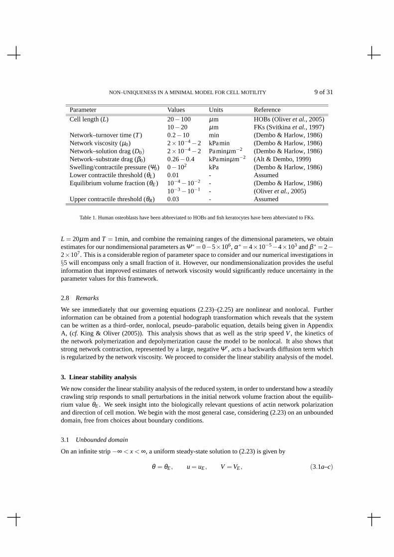
Parameter Values Units Reference

Cell length (L) 20−100 µm HOBs (Oliveret al., 2005)10−20 µm FKs (Svitkinaet al., 1997)

Network–turnover time (T) 0.2−10 min (Dembo & Harlow, 1986)Network viscosity (µ0) 2×10−4−2 kPamin (Dembo & Harlow, 1986)Network–solution drag (D0) 2×10−4−2 Paminµm−2 (Dembo & Harlow, 1986)Network–substrate drag (β0) 0.26−0.4 kPaminµm−2 (Alt & Dembo, 1999)Swelling/contractile pressure (Ψ0) 0−102 kPa (Dembo & Harlow, 1986)Lower contractile threshold (θL) 0.01 - AssumedEquilibrium volume fraction (θE) 10−4−10−2 - (Dembo & Harlow, 1986)

10−3−10−1 - (Oliver et al., 2005)Upper contractile threshold (θR) 0.03 - Assumed

Table 1. Human osteoblasts have been abbreviated to HOBs andfish keratocytes have been abbreviated to FKs.

L = 20µm andT = 1min, and combine the remaining ranges of the dimensional parameters, we obtainestimates for our nondimensional parameters asΨ∗ = 0−5×106, α ∗ = 4×10−5−4×103 andβ∗ = 2−2×107. This is a considerable region of parameter space to consider and our numerical investigations in§5 will encompass only a small fraction of it. However, our nondimensionalization provides the usefulinformation that improved estimates of network viscosity would significantly reduce uncertainty in theparameter values for this framework.

2.8 Remarks

We see immediately that our governing equations (2.23)–(2.25) are nonlinear and nonlocal. Furtherinformation can be obtained from a potential hodograph transformation which reveals that the systemcan be written as a third–order, nonlocal, pseudo–parabolic equation, details being given in AppendixA, (cf. King & Oliver (2005)). This analysis shows that as well as thestrip speedV, the kinetics ofthe network polymerization and depolymerization cause themodel to be nonlocal. It also shows thatstrong network contraction, represented by a large, negativeΨ ′, acts a backwards diffusion term whichis regularized by the network viscosity. We proceed to consider the linear stability analysis of the model.

3. Linear stability analysis

We now consider the linear stability analysis of the reducedsystem, in order to understand how a steadilycrawling strip responds to small perturbations in the initial network volume fraction about the equilib-rium valueθE. We seek insight into the biologically relevant questions of actin network polarizationand direction of cell motion. We begin with the most general case, considering (2.23) on an unboundeddomain, free from choices about boundary conditions.

3.1 Unbounded domain

On an infinite strip−∞ < x< ∞, a uniform steady-state solution to (2.23) is given by

θ = θE, u= uE, V =VE, (3.1a–c)

10 of 31 L.S. GALLIMORE et.al.

for any positive constantVE, provided

J(θE) = 0, uE =−β(θE)VE

α (θE)+β(θE); (3.2a,b)

hereafter we will use a subscriptE on a constitutive law to indicate that it is evaluated at the equilibriumnetwork volume fractionθE, i.e. αE = α (θE) and so on. Note the constraint placed onJ is satisfied by(2.5). In the usual way we seek a solution to (2.23) by linearizing about (3.1) as follows

θ ∼ θE + εθ1+ · · · , u∼ uE + εu1+ · · · , V ∼VE + εV1+ · · · , (3.3a–c)

whereε ≪ 1 is a small parameter associated with small prescribed variations in the initial networkvolume fraction. We obtain atO(ε) the linearized system

∂θ1

∂ t+uE

∂θ1

∂x+θE

∂u1

∂x=−J′Eθ1, (3.4)

−Ψ ′E

∂θ1

∂x+µE

∂ 2u1

∂x2 = αEu1+βE(u1+V1)+(α ′EuE +β ′

E(uE +VE))θ1, (3.5)

where a prime′ on a constitutive law indicates its derivative with respectto θ, so thatα ′E = dα/dθ(θE)

and so on. Differentiating (3.5) oncew.r.t. x, then eliminatingu1 using (3.4) shows that small distur-bances in the network volume fraction are governed by the linear partial differential equation

(

∂∂ t

+uE∂∂x

+J′E

)(

θ1−µE

(αE +βE)

∂ 2θ1

∂x2

)

+γEuE∂θ1

∂x=

θEΨ ′E

(αE +βE)

∂ 2θ1

∂x2 , (3.6)

for θ1, where

γE =−θE

(αE +βE)

(

α ′E +β ′

E

(

1+VE

uE

))

=−θEβE

(αE +βE)

(

αβ

)′

E. (3.7)

Equation (3.6) has pseudo–parabolic character through the∂ 3θ1/∂x2∂ t and also contains a third spatialderivative. Thus the network is convected with velocity(1+ γE)uE, where the parameterγE capturesthe net effect on the linearized problem of network–solution drag and adhesion. Seeking a solution to(3.6) of the formθ1(x, t) = Re[θ1exp(ikx+Ω (k)t)], whereθ1 is a complex constant, leads immediatelyto the dispersion relation (cf. Demboet al. (1984))

Ω (k) =−J′E −θEΨ ′

Ek2

αE +βE +µEk2 − ikuE

(

1+(αE +βE)γE

αE +βE +µEk2

)

, (3.8)

for Ω (k), the growth rate of a small, spatially periodic perturbation of wavenumberk (wherek is takento be non-negative without loss of generality). The corresponding perturbation in the network velocityis given by

u1 =θ1

θE

(

(αE +βE)γEuE −θEΨ ′Eik

αE +βE +µEk2

)

exp(ikx+Ω (k)t). (3.9)

Thus, in general small perturbations inθ andu have different amplitudes and are not in phase.

NON–UNIQUENESS IN A MINIMAL MODEL FOR CELL MOTILITY 11 of 31

0kc

k

−J′

E

k

(a) J ′

E = 0 (b) J ′

E > 0

0

Ω∞ > 0

Ω∞ = 0

Ω∞ < 0

Re(Ω(k))

Ω∞ > 0

Ω∞ = 0

Ω∞ < 0

Re(Ω(k))

FIG. 2. Plots of the typical growth rates given by (3.8) in the cases (a)J′E = 0 and (b)J′E > 0, whereΩ∞ andkc are given by (3.10)and (3.11); see text for details.

We consider separately the two cases (a)J′E = 0 and (b)J′E > 0, the first being relevant to the specialcase in which there is no mass transfer (i.e. J≡ 0) and the second to the constitutive law (2.27a) (forwhichJ′E = 1). We begin by noting that (i)Re(Ω (0)) =−J′E, (ii) Re(Ω (k))→ Ω∞ ask→ ∞, where

Ω∞ :=−

(

J′E +θEΨ ′

E

µE

)

(3.10)

and (iii) Re(Ω (k)) is monotonic increasing (decreasing) forΩ∞ >−J′E (Ω∞ <−J′E). Linear instabilityensues if and only if Re(Ω (k)) > 0 for some wavenumberk > 0. We identify three regimes in bothcases (a) and (b) depending on the sign ofΩ∞, as illustrated in Figure 2. In case (a), perturbations withk> 0 are linearly stable (unstable) forΩ∞ < 0 (Ω∞ > 0); the neutral-stability point lies atk= 0 in bothof these regimes, which are separated by the borderline regime (Ω∞ = 0) in which all perturbations areneutrally stable. In case (b), all perturbations are stablefor Ω∞ < 0; in the borderline regime in whichΩ∞ = 0, the point of neutral stability lies atk= ∞ and finite wavenumber perturbations are stable; in thethird regime, which pertains forΩ∞ > 0, the point of neutral stability is given by

k= kc :=

(

(αE +βE)J′EµEΩ∞

)1/2

, (3.11)

so perturbations grow (decay) for all wavenumbersk> kc (k< kc).We note that the mass transfer term stabilizes long wavelength perturbations forJ′E > 0. The

swelling/contractile pressure is the only destabilizing term, withΩ∞ being positive for sufficiently largeand negativeΨ ′

E, i.e. for Ψ ′E <−µEJ′E/θE. The phase speed is independent ofJ′E and given by

c(k) :=−Im(Ω (k))

k= uE

(

1+(αE +βE)γE

αE +βE +µEk2

)

, (3.12)

so modes propagate downstream (upstream) forγE > 0 (γE < 0) at a speed that decreases with thewavenumber, a property that may be pertinent to the ruffling behaviour of pseudopodia. We note thatγE < 0 for the constitutive laws (2.28d,e). We also note that the swelling/contractile pressure featuresin the growth rate (3.8), but not in the phase speed (3.12), because it drives diffusive transport of thenetwork up and down its density gradient.

12 of 31 L.S. GALLIMORE et.al.

3.2 Effect of boundary conditions

We now consider the effect of imposing the boundary conditionsu(0, t) = u(1, t) = 0 and see that aftersubstituting (3.3) into (2.23) we obtain, atO(ε), (3.4) and (3.5) withuE = VE = 0. Thus the speed atwhich the strip travels is now of the same order as the initialperturbation in network volume fractionaboutθE. We seek solutions of the formθ1 = θ1(x)eωt , u1 = u1(x)eωt , V1 = V1eωt , which after droppingthe hats and eliminatingθ1 gives

(

θEΨ ′E

J′E +ω+µE

)

d2u1

dx2 − (αE +βE)u1 = βEV1, (3.13)

for J′E +ω 6= 0. (ForθE 6= 0 andΨ ′E 6= 0, J′E +ω = 0 only atk = 0.) ForV1 = 0 this becomes a linear,

homogeneous, second-order system, leading to solutions ofthe form

u1 = Asin(nπx)eωnt , θ1 =−AnπθE

J′E +ωncos(nπx)eωnt , (3.14a,b)

for n an integer, where the growth rate is in agreement with (3.8),so thatωn = Ω (nπ) with uE = 0; A isa constant and the linearized form of (2.25), namely

〈βE(u1+V1)〉= 0, (3.15)

implies thatn is even. Thus, small perturbations to the network volume fraction aboutθE, that aresymmetric aboutx= 1/2 do not cause the strip to move. ForV1 6= 0 in (3.13) the solutions are given by

u1 =V1βE

αE +βE

(

cos(λn(x−1/2))cos(λn/2)

−1

)

eω(λn)t , θ1 =V1βEθEλn

(αE +βE)(J′E +ω(λn))

sin(λn(x−1/2))cos(λn/2)

eω(λn)t ,

(3.16a,b)where again the growth rates are in agreement with (3.8) andω(λn) = Ω (λn) for uE = 0. It remains todetermineλn, by substitutingu1 from (3.16a) into the linearized version of (2.25). We find thatλn is theroot of

αE

βE+

2λn

tan

(

λn

2

)

= 0, (3.17)

such that(2n− 1)π < λn < 2πn. We note that the boundary conditions do not alter the growthratecurves depicted in Figure 2 – they simply identify a discreteset of points on these curves. The growthrate curve plateaus and remains in the unstable regime for large wavenumbers, whenΩ∞ > 0, so thesolution leaving the linear regime depends on how the coefficients of the short wavelength modes in theinitial perturbation depend on the wavenumber. The fact that small perturbations to the network, aboutits equilibrium volume fraction, only cause the strip to move if they break the symmetry of the networkis an interesting insight into the polarization of the network in crawling cells.

3.3 Solution of the linearized initial value problem

It is possible to show by direct calculation, using (3.17), that theθ1 modes in (3.14b) and (3.16b) areorthogonal. Working with these modes we seek to understand how the strip travels in response to ageneral small perturbation of the network about the equilibrium volume fraction. We seek a solution ofthe form

θ1(x, t) =a0(t)

2+ ∑

nevenan(t)cos(nπx)+

∞

∑n=1

bn(t)sin(λn(x−1/2))

cos(λn/2), (3.18)

NON–UNIQUENESS IN A MINIMAL MODEL FOR CELL MOTILITY 13 of 31

where theλn are given by (3.17) and following (3.3a) we expand the initial conditionθ∗ ∼ θE + εθ∗1 +

· · · so that

an(0) = 2∫ 1

0θ∗

1 (ξ )cos(nπξ)dξ , bn(0) =2λncos(λn/2)λn−sin(λn)

∫ 1

0θ∗

1 (ξ )sin(λn(ξ −1/2))dξ .

(3.19a,b)Substituting (3.18) into (3.6) withuE = 0 and using orthogonality to equate the coefficients of like terms,we find that

a0+J′Ea0 = 0, (3.20)

for n even(αE +βE +µEn2π2)an+J′E(αE +βE +µEn2π2)an =−θEΨ ′

En2π2an, (3.21)

and forn an integer

(αE +βE +µEλ 2n π2)bn+J′E(αE +βE +µEλ 2

n π2)bn =−θEΨ ′Eλ 2

n π2bn. (3.22)

After some manipulation we see that

for n even, an(t) = an(0)eωnt ; for integern, bn(t) = bn(0)e

ω(λn)t , (3.23a,b)

where of course, in agreement with (3.8),ωn = Ω (nπ) andω(λn) = Ω (λn), both with uE = 0. Nowwe substitute (3.18) into (3.4) withuE = 0, integrate and apply the boundary conditions thatu1 = 0 atx= 0,1 to find

u1 =∞

∑n=1

J′E +ωλn

λnθEbn(t)

(

cos(λn(x−1/2))cos(λn/2)

−1

)

− ∑neven

J′E +ωn

nπθEan(t)sin(nπx), (3.24)

which we substitute into (3.5) along with (3.18) to obtain, after some manipulation, the linear predictionfor the crawling speed of the strip in terms of the initial conditions and the model parameters in the form

V1 =−Ψ ′

E(αE +βE)

βE

∞

∑n=1

λnbn(0)eω(λn)t

αE +βE +µEλ 2n. (3.25)

This expression is verified against our numerics in§5. We again see that only the perturbations tothe network that are asymmetric aboutx = 1/2 contribute, viabn, to the speed of the crawling strip.Having found an expression for the moving–strip speed in terms of a small perturbation to the networkequilibrium volume fractionθE, one might anticipate we could make some general statement about thedirection in which a stationary strip of cytoplasm starts tocrawl when disturbed. However, the flatteningof the growth rate curve for large wavenumber leads to an expression forV1 that depends on how thelarge wavenumber modes are excited. All the large wavenumber modes grow at a comparable rate, sothe initial amplitude of each mode is important in determining which mode dominates as the solutionexits the linear regime. The implication for modelling cellcrawling is that the perturbation responsedisplayed by this deterministic model is rich and depends onboth the modes that are excited, theirrelative amplitudes and the symmetry of the perturbation.

An alternative approach is to write the initial conditionθ∗1 as a Fourier cosine series, which is

advantageous because completeness of the Fourier modes is well known. The resulting calculation forV1 is presented in Appendix B. It is somewhat more involved, dueto the coupling of the Fourier modes

14 of 31 L.S. GALLIMORE et.al.

that are asymmetric aboutx = 1/2. For example, an initial perturbationθ∗1 = cos(nπx), for n odd,

corresponds to the following infinite sum for the travelling–strip speed

V1(t) =−2Ψ ′

E(αE +βE)

βE(αE +βE +µEn2π2)

eωnt

f (ωn)+

∞

∑k=1

eω(λk)t

(ω(λk)−ωn) f ′(ω(λk))

, (3.26)

where f is defined in Appendix B. It can be shown (see Appendix B) that (3.25) agrees with the Fourierseries expression derived forV1 and so we claim that the modes used to construct (3.18) are complete.

4. Small growth rate limit

We now consider a parameter limit in which we can say a little more about the early response of themodel to a small perturbation to the stationary steady state, namely the parameter regime in which themaximum growth rate is small and positivei.e.0<Ω∞ ≪ 1. Note this is different to a traditional weaklynonlinear analysis, because we are unable to isolate and excite only the fastest growing mode. We tacklethis regime in general, without prescribingΨ explicitly, by parametrizingΨ with Ω∞. Now, definingε = Ω∞ for convenience, (3.10) pertains provided

∂Ψ∂θ

(θE;ε) =−µE

θE

(

J′E + ε)

. (4.1)

We fix kc = O(1), so assumingJ′E = O(1), (3.11) shows we must rescale

α = εα , β = εβ , (4.2a,b)

so we consider a small network–solution drag and small adhesion limit. Hereafter, we drop the hats.

4.1 Small time problem t= O(1)

We begin by considering the early evolution on the time–scale t = O(1), substituting (4.2) into thegoverning equations (2.23) and dropping the hats we obtain

θt +(θu)x =−J, −Ψx(θ;ε)+(

µux)

x = ε(

αu+β(u+V))

. (4.3a,b)

We Taylor expand the swelling/contractile pressure,Ψ, and use asymptotic series expansionsθ ∼ θE +εθ1+ ε2θ2+ · · · , u∼ εu1+ ε2u2+ · · · andV ∼ εV1+ ε2V2+ · · · , to obtain at O(ε)

∂θ1

∂ t+θE

∂u1

∂x=−J′Eθ1,

µEJ′EθE

∂θ1

∂x+µE

∂ 2u1

∂x2 = 0. (4.4a,b)

Integrating the first equation once and the second twicew.r.t. x (usingu1 = 0 atx= 0,1) then manipu-lating and integratingw.r.t. t reveals that

θ1(x, t)−〈θ1〉(t) = θ∗1 (x)−〈θ∗

1〉, 〈θ1〉(t) = 〈θ∗1 〉e

−J′Et . (4.5a,b)

Hence we see our choice of nondimensional time–scale (2.20)returned as the time–scale over whichrelaxation of the network, via polymerization and depolymerization, occurs. There is no leading order

NON–UNIQUENESS IN A MINIMAL MODEL FOR CELL MOTILITY 15 of 31

change in shape of the network profile. Moreover, the networkvelocity is independent oft, as is themoving-strip velocity

u1(x, t) =−J′EθE

(

∫ x

0θ∗

1 (ξ )dξ −x〈θ∗1 〉

)

, V1(t) = V (θ∗1) =

J′EθE

(

〈〈θ∗1〉〉−

12〈θ∗

1 〉

)

, (4.6a,b)

where, here and hereafter

〈〈θ∗1〉〉 :=

∫ 1

0

∫ x

0θ∗

1 (ξ )dξ dx. (4.7)

In this parameter regime the initial speed of the moving strip is constant and depends only on howθ∗

varies along the strip from the mean ofθ∗. Loosely speaking, if one side of the strip has a higher thanmean network volume fraction and the other side of the strip has a lower than mean volume fraction,then the side with the higher volume fraction becomes the rear of the strip.

4.2 Large time problem t= O(1/ε)

By our choice of parameter regime the growth rate is of O(ε), so perturbations to the network evolveslowly. Here we investigate them on the long time–scalet = τ/ε, with τ =O(1), for which the governingequations (2.23) become

εθτ +(θu)x =−J, −Ψx(θ;ε)+(

µux)

x = ε(

αu+β(u+V))

. (4.8a,b)

We expandθ ∼ θE+εθ1+ε2θ2+ · · · , u∼ εu1+ε2u2+ · · · andV ∼ εV1+ε2V2+ · · · , as in the previoussection and obtain at O(ε), after rearranging

θ1 =−θE

J′E

∂ u1

∂x, (4.9)

as well as the derivative of this equation with respect tox. In this form it reflects how the flow ofthe network changes the local network volume fraction. The derivative represents a balance betweenswelling/contractile forces and viscous forces. Since thesolution remains incompletely specified, wemust proceed to second order to determine the second solvability condition for θ1 andu1.

At second-order, after some manipulation, we obtain the expressions

−

(

J′Eθ2+θE∂ u2

∂x

)

=∂ θ1

∂τ+

∂∂x

(

θ1u1)

+12

J′′Eθ 21 , (4.10)

−µE∂∂x

(

J′Eθ2+θE∂ u2

∂x

)

=∂∂x

(

µEθ1−12

θEΨ ′′E θ 2

1 +θEµ ′Eθ1

∂ u1

∂x

)

−θE(

αEu1+βE(u1+V1))

,

(4.11)

whereΨ ′′E =Ψθθ(θE;0). Differentiating the first of these expressions with respect to x and substituting

it into the second, we obtain the second solvability condition

µE∂∂x

(

∂ θ1

∂τ+

∂∂x

(

θ1u1)

+12

J′′Eθ 21

)

=

∂∂x

(

µEθ1−12

θEΨ ′′E θ 2

1 +θEµ ′Eθ1

∂ u1

∂x

)

−θE(

αEu1+βE(u1+V1))

, (4.12)

16 of 31 L.S. GALLIMORE et.al.

for θ1 andu1. Using (4.9) to eliminateθ1 from (4.12), we obtain the pseudo–parabolic equation

∂∂x

∂∂x

(

∂ u1

∂τ+ u1

∂ u1

∂x− u1

)

−aE

(

∂ u1

∂x

)2

= bE(

αEu1+βE(u1+V1))

, (4.13)

for u1(x,τ ), where

aE =θE

2µEJ′E

(

θEΨ ′′E +µEJ′′E +2µ ′

EJ′E)

, bE =J′EµE

. (4.14a,b)

For the moving–strip problem, matching with the small time solutions in the previous section yieldsthe initial condition

limτ→0

θ1(x,τ ) = limt→∞

θ1(x, t) = θ∗1 (x)−〈θ∗

1〉. (4.15)

We note that (4.9) is consistent with the homogeneous Dirichlet conditions for ˆu1 if and only if 〈θ1〉= 0,a condition that is satisfied by the initial conditions (4.15), but not by arbitrary initial conditions withnonzero mean, which highlights the need for thet =O(1) analysis. The corresponding ‘initial condition’for (4.13) is given by (4.6a). The solvability condition (2.25) implies that〈u1+V1〉= 0, and hence, by(4.9), that

V1(τ ) =−〈u1(x,τ )〉=J′EθE

〈〈θ1(ξ ,τ )〉〉; (4.16)

this expression is consistent with the small-time analysisbecauseV1(τ ) ∼ V (θ∗) asτ → 0 by (4.15),whereV (θ∗) is given by (4.6b). We see that the moving–strip speed is no longer constant and dependson the network velocity. Unfortunately the nonlinear, pseudo–parabolic equation (4.13) controllingu1 does not represent a significant simplification of the full problem, so making predictions about themotion of the travelling strip and the evolution of its network, without simulating numerically, would beinvolved. We also note that in that if we setaE = bE = 0, (4.13) reduces to the forced, inviscid Burgers’equation. This small growth rate analysis is verified against numerical solutions in the appropriateparameter regime in Appendix C.

5. Numerical simulations

5.1 Description of the scheme

We obtain numerical solutions to (2.23)–(2.25) with a fullycoupled finite element scheme (see, forexample, Eriksson (1996)), with the resulting discretisedsystem of nonlinear algebraic equations solvedusing the PETSc libraries, (Balayet al., 1997, 2010, 2011). The scheme uses a piecewise linear basisfor the spatial approximations and on each time step the solution at the previous time step is used as aninitial guess for the Newton iteration used to solve the nonlinear system. The scheme is fully implicitin time. We prescribe initial conditions for network distribution, such that〈θ∗〉 = θE and solve theunsteady problem on the interval[0,1] for the network profile, network velocity and strip speed. Afterdemonstrating the code’s convergence in both space and time(see Appendix D), we also validated itagainst our linear stability analysis.

5.2 Results

We first consider the solution to the initial value problem (2.23)–(2.25), with parameter valuesΨ∗ =15,000, α ∗ = 0.4 andβ∗ = 3. The initial conditions are a small perturbation to the uniform steady

NON–UNIQUENESS IN A MINIMAL MODEL FOR CELL MOTILITY 17 of 31

state, such thatθ∗(x) = θE + ε cos(πx) with ε = 10−4. Figure 3 shows how the speed of the travellingstrip increases from near stationary and oscillates, before settling to a constant speed. We also plot thelinear stability prediction, (3.25), which holds for smalltimes (i.e. until the perturbation to the steadystate grows and exceeds the linear regime). The initial conditions have an elevated network volume

0 20 40 600

0.02

0.04

0.06

0.08

0.1

Numerical solution

Linear prediction

V

t

FIG. 3. Speed of the travelling strip and comparison to linear stability predictions. The parameters used areΨ∗ = 15,000,α ∗ = 0.4andβ∗ = 3 and the initial condition is a perturbation to the equilibrium volume fraction: see text. Network volume fraction andvelocity are plotted for the boxed times in Figure 4.

fraction atx= 0 and the network is in the contractile regime (θL < θ < θR) so the network flows up theconcentration gradient towardsx= 0. The strip starts to crawl in the direction opposite to thatin whichthe network is flowing, so the model displays the biologically observed behaviour of treadmilling on thescale of the strip. The peak in network volume fraction is thus located at the rear of the travelling strip.The network dips at the front of the travelling strip. We plotsnapshots of the network volume fractionand velocity in Figure 4, at the times indicated by the boxes in Figure 3. Once the travelling strip ineffect attains a constant speed the network volume fractionand velocity are also constant in time and ourunsteady code has found a steady travelling–wave solution as the large–time attractor. We shall proceedto consider when such travelling waves can be found and how they depend on the model parameters.

5.3 Effect of adhesion strength

Our numerical experiments have indicated that the travelling strip attains a steady travelling wave for awide range of parameters, although there are a number of qualitatively distinct forms the travelling wavecan take. The top three rows of Figure 5 show travelling–wavesolutions with one, two and three peaksin the network volume fraction. These peaks are regions where substantial flow of the network up itsconcentration gradient has formed a large gradient in network volume fraction. The peak is preventedfrom growing further once the volume fraction exceeds the contractile regime (θ > θR) and networkswelling resists contraction. The bottom row of Figure 5 contains a slightly different travelling–wave

18 of 31 L.S. GALLIMORE et.al.

0 0.2 0.4 0.6 0.8 1−0.14

−0.12

−0.1

−0.08

−0.06

−0.04

−0.02

0

0 0.2 0.4 0.6 0.8 1

0.015

0.02

0.025

0.03

t=3t=6t=9t=12t=24t=60 uθ

x x(a) (b)

FIG. 4. Snapshots of the network volume fraction (a) and velocity (b) at the times indicated by the boxes in Figure 3. Theparameters used areΨ∗ = 15,000,α ∗ = 0.4 andβ∗ = 3.

solution which has a peak at both ends of the travelling strip. The first column displays the networkvolume fraction, colour coded to identify swelling or contracting and polymerizing or depolymerizingregions of the strip. The central column shows variation in hydrodynamic pressure and mixture stressacross the strip. We note that for all four travelling–wave solutions the pressure is largest at the rear ofthe strip and decreases towards the front. The mixture stress oscillates, with a local maximum just infront of each of the network volume fraction peaks. The final column shows the network and solutionvelocities, in the frame that travels with the strip. The network flows backwards displaying treadmilling,whilst the solution flows forwards much more slowly. At each of the interior peaks in network volumefraction and at the front of the split peak solution, there isa small region where the network flowsforwards.

Some of the numerical simulations generated travelling–wave solutions with a negative crawlingspeedV. We note that for any solution the transformation(θ(x),u(x),V)→ (θ(1−x),−u(1−x),−V)yields another solution. Since, in this section, we are concerned with travelling–wave solutions andnot transient behaviour, any numerical solution obtained with negativeV has been transformed to thecorresponding positiveV solution before plotting it in either Figure 5 or Figure 6.

The effect of adhesion strengthβ∗ on the speed of the travelling stripV is shown in Figure 6 forfixed contractile strengthΨ∗ = 15,000 and network–solution dragα ∗ = 0.4. To reduce the time takenfor a simulation to attain a steady state, we have employed continuation. The steady state network pro-file obtained in Figure 4 was used as the first point on the one peak curve and the initial condition forthe problems with a slightly smaller and largerβ∗. The first solutions in each of the other qualitativelydistinct families were obtained when the continuation failed,i.e. the final network profile from a simula-tion that had not settled to a steady state was used as the initial condition to the problem with a differentβ∗. The solutions plotted in Figure 6 were all calculated on grids with five thousand and ten thousandelements and the largest relative error in steady strip speed was 7.1×10−3.

We notice first that the qualitatively distinct families of solutions overlap in parameter space, so fora given set of parameters different initial conditions can yield different, non–trivial, steady, travellingsolutions. We also note the bell–shaped dependence of speedon adhesion strength displayed withineach family. As the number of peaks increases, the speed drops and the bell–shaped curve flattens for

NON–UNIQUENESS IN A MINIMAL MODEL FOR CELL MOTILITY 19 of 31

0 0.2 0.4 0.6 0.8 1

0.015

0.02

0.025

0.03

0.035

0 0.2 0.4 0.6 0.8 1−0.06

−0.05

−0.04

−0.03

−0.02

−0.01

0

0.01

0 0.2 0.4 0.6 0.8 1

0.015

0.02

0.025

0.03

0.035

0 0.2 0.4 0.6 0.8 1−0.04

−0.03

−0.02

−0.01

0

0.01

0 0.2 0.4 0.6 0.8 1

0.015

0.02

0.025

0.03

0.035

0 0.2 0.4 0.6 0.8 1

−0.1

−0.08

−0.06

−0.04

−0.02

0

0 0.2 0.4 0.6 0.8 1−0.1

−0.08

−0.06

−0.04

−0.02

0

0 0.2 0.4 0.6 0.8 1

0.015

0.02

0.025

0.03

0.035

0 0.2 0.4 0.6 0.8 1−0.012

−0.0118

−0.0116

−0.0114

0 0.2 0.4 0.6 0.8 1−5

0

5

10x 10

−4

0 0.2 0.4 0.6 0.8 1−0.012

−0.0119

−0.0118

−0.0117

0 0.2 0.4 0.6 0.8 1−1

0

1

2x 10

−3

0 0.2 0.4 0.6 0.8 1−0.0116

−0.0114

−0.0112

−0.011

0 0.2 0.4 0.6 0.8 1−1

0

1

2x 10

−3

0 0.2 0.4 0.6 0.8 1−0.012

−0.0119

−0.0118

−0.0117

−0.0116

0 0.2 0.4 0.6 0.8 1−5

0

5

10

15x 10

−4

One peak β∗ = 4, V = 0.0661

Two peaks β∗ = 21, V = 0.0320

Three peaks β∗ = 44, V = 0.0208

Split peak β∗ = 9, V = 0.0581

x x x

xxx

x

x

x x

xx

u, v

u, v

u, v

u, v

σ

σ

σ

σ

p

p

p

p

4

4

3

3

θ

θ

θ

θ

FIG. 5. Steady state plots for a range of differentβ∗ values withΨ∗ = 15,000,α ∗ = 0.4. The speedV is stated to three significantfigures. For all these simulationsV > 0, sox= 0 is the rear of the travelling strip. The first column displays the network volumefraction (shading: white is swelling and depolymerizing; light grey is contracting and depolymerizing; mid grey is contractingand polymerizing: see (2.5), (2.6) and Figure 1.) The middlecolumn displays the hydrodynamic pressurep (continuous, left axis)and mixture stressσ (dashed, right axis). The final column shows the network velocity u (continuous) and the solution velocityv (dashed), both in a frame that travels with the strip. The boxon the peak in network volume fraction forβ∗ = 21 indicates thezoomed region (not to scale) displayed in Figure 10 in Appendix D.

20 of 31 L.S. GALLIMORE et.al.

10−2

100

102

0.01

0.02

0.03

0.04

0.05

0.06

0.07

One peak

Two peaks

Three peaks

Split peaks

Adhesion β∗

SpeedV

FIG. 6. Travelling speed of steady states as a function of adhesion strength, typical solutions for each family of points canbe seenin Figure 5. The parameters used areΨ∗ = 15,000 andα ∗ = 0.4.

the one, two and three peak families. Within the family of split peaks, as we increase cell–substrateadhesion,β∗, the actin peak at the front narrows substantially. For smaller, decreasingβ∗ values thespeed of the split peak solution decreases rapidly as the profile becomes more symmetric. This may beinterpreted as cells that do not have a strongly defined polarity travelling more slowly.

5.4 Remarks

Finding numerical solutions to (2.23)–(2.25) has proved more computationally expensive than one mightanticipate for a one–dimensional problem, not least because of sharp peaks in network volume fractionthat dance in the transient solutions, before settling to a steady state. Preliminary numerical investiga-tions found some steady travelling–wave solutions with more than three peaks in the network profile,for different parameter values and initial conditions of a small perturbation to the equilibrium networkvolume fraction. We are confident that the results of numerical simulations displayed here have suf-ficient resolution to capture the actin peaks – see Appendix D. Moving actin peaks have previouslybeen seen in other models within this framework, (e.g.Demboet al. (1984); Alt & Dembo (1999)) andmay be relevant to the ruffling phenomena observed in cells. Many of the transient solutions displayedoscillations inV around a constant. We took great care to understand whether these oscillations werea numerical artefact (amplitude reduced by spatial refinement), a slowly decaying transient (amplitudedecreases with time) or a true oscillation (amplitude persists when the simulation is run for longer andis unaffected by spatial and temporal refinement.) Only whenthe relative amplitude of the oscillation isless than 9.1×10−4 for at least the final twenty nondimensional time units of thesimulation have weaccepted the solution as settled to a steady state.

Since all our solutions are obtained with an unsteady code, we reason that they must be stable tosufficiently small perturbations. Our intuitive understanding based on running simulations is for moreextremeβ∗ values within a given family, smaller steps in the continuation parameterβ∗ are requiredin order for the simulation to settle to a steady state in a reasonable amount of time. In some of the

NON–UNIQUENESS IN A MINIMAL MODEL FOR CELL MOTILITY 21 of 31

overlap regions, too large a step inβ∗ causes the code to settle on a steady state solution belonging to adifferent family. In some cases the transient solution is sosensitive to the initial conditions that simplytruncating theθ values associated with the steady state (to say, five significant figures) and feeding themback in as initial conditions causes the moving–strip velocity to grow away from its steady velocity, aftera short lag, and then oscillate before returning to the original steady state. For some of the split peaktravelling–wave solutions, a steady state, withV positive, generated on the coarser grid (5000 elements)and used as initial conditions on the finer grid (10,000 elements) results in a simulation which changesdirection and settles to the corresponding steady state withV negative. These simulations were includedas converged in Figure 6 as discussed in§5.3.

6. Discussion

We have presented stability analyses and numerical simulations for a stripped–down, two–phase, poro-viscous, reactive flow model applicable to cell crawling. The linear stability analysis about a uniform,stationary state predicts an initial crawling direction that depends both which modes are excited and therelative amplitude of these modes in the initial perturbation. It also provides a mechanism by whichan asymmetric perturbation is required to cause the strip totravel, suggesting this framework could beuseful in explaining the polarization of crawling cells. This analysis was done for general constitutivelaws and the positive plateauing growth rate for large wavenumbers is obtained as long asΨ ′

E < 0, so wewould expect similar results for different constitutive laws in this class. Numerical investigations intothe effect of adhesion strength on cell speed found familiesof travelling–wave solutions, with each fam-ily displaying the bell–shaped dependence of speed on adhesion strength that has been experimentallyobserved, (seee.g.Paleceket al. (1997)). To our knowledge this has not previously been demonstratedin the two–phase flow framework for such a simple model, although it has been found in viscoelasticmodels for crawling cells (DiMillaet al., 1991; Gracheva & Othmer, 2004) and in a more complicatedmodel that uses the two–phase flow framework (Altet al., 2010).

The network velocities associated with our travelling states also display the experimentally observedphenomenon of treadmilling. Whilst we have not explicitly modelled the transport of actin monomers,the flow of solution carries them forwards, making them available for network polymerization. Acrossthe one, two and three peak solutions the actin volume fraction dips at the front of the cell. By con-struction, the network undergoes net polymerization wherever the network volume fraction is below theequilibrium valueθE. Therefore whilst these solutions display strong polymerization at the cell front inagreement with experiments, they cannot also capture the high actin densities observed at the front oftravelling cells. This could be corrected in subsequent models by allowing a mass transfer between thenetwork and solution phases to occur on the boundary. The actin distribution in the split peak familyof solutions is very interesting: this solution could be biologically relevant to modelling cell motility,specifically the lamellipodium, which has a high actin density both at the leading edge and the transitionto the cell body (Svitkinaet al., 1997). That the actin profile declines so sharply behind thefront peakallows polymerization to take place close to the front of thetravelling strip.

Due to the increased computational cost of resolving more peaks we limited our study of the effectof adhesion strength to three peak solutions. However, it isprobable that families of travelling–wavesolutions with more than three peaks exist. It also remains to determine whether the families of stablesolutions displayed in Figure 6 extend further and could be found by allowing the code more time toreach steady state, or whether there are some bifurcation points for the parameterβ∗ beyond which thestable steady solutions become unstable or do not exist. A complete characterisation of the steady statesolutions, including unstable solutions and the domains ofattraction for the stable solutions remains an

22 of 31 L.S. GALLIMORE et.al.

open problem.Previous studies of similar systems have suggested the system may be chaotic. We have some

simulations in which many peaks in the network volume fraction emerge, grow, move, merge and displaywhat appears to be very complicated behaviour, particularly asΨ∗ increases. However, when we havepursued these simulations we have found that the complicated behaviour is an artefact of a poorlyconverged simulation. Of course this does not preclude the existence of chaos in the system, we simplyhave not found good evidence for it. This paper provides a fewnumerical examples to demonstrate thestructure of some steady state solutions in parameter space, future work might attempt a more thoroughinvestigation of parameter space and a characterisation ofthe transient solutions, in particular lookingfor any periodic in time solutions which may exist.

It would also be interesting to consider a two–dimensional version of this model. We believe that theplateauing growth rate is responsible for many of the exciting features of this model and it remains aninteresting open problem to understand how this growth rateis modified by the inclusion of additionalphysical or biological phenomena. We know for instance thatcoupling a reaction, advection, diffusionequation to the model, for some species, say myosin, that is advected with the network, stabilises largewavenumbers. How different network rheologies would alterthe growth rate is something we intend toinvestigate further. In short, two–phase flow models have many intrinsic features relevant to cell motilitydescribed here, and surely many more surprises yet to be uncovered.

Acknowledgements

We would like to thank Jonathan Ratcliffe, Colin Scotchfordand David Grant at the University of Not-tingham and Hans Othmer at the University of Minnesota for very helpful discussions. This publicationis based on work supported in part by Award No. KUK-C1-013-04, made by King Abdullah Universityof Science and Technology (KAUST). SLW is grateful for funding from the EPSRC in the form of anAdvanced Research Fellowship and JRK for that of the WolfsonFoundation and Royal Society.

A. Potential hodograph transformation

In the travelling frame, the amount of network in the strip between the origin and the pointx> 0 is givenby

m(x, t) =∫ x

0θ(ξ , t)dξ . (A.1)

If θ(x, t) is continuous and strictly positive,m(x, t) is strictly increasing and continuous, which guaran-tees the existence of its inverse,x= χ(m, t) say. The idea behind the potential hodograph transformationis to use this expression to replace the independent variable x in the governing equations with the newindependent variablem. As we shall see this leads to some useful insight.

A.1 Formulation

For concreteness we define the integrated mass variablem for the network phase by setting

m=

∫ χ(m,t)

0θ(ξ , t)dξ , χ(0, t) = 0, (A.2a,b)

and make the change of variables fromx to m by writing

θ(χ(m, t), t) =Θ(m, t), u(χ(m, t), t) =U(m, t). (A.3a,b)

NON–UNIQUENESS IN A MINIMAL MODEL FOR CELL MOTILITY 23 of 31

Sinceθ is continuous and strictly positive,χ(m, t) is differentiable and (A.2a) gives

1= θ(χ(m, t), t)∂ χ∂m

(m, t), 0=

∫ χ(m,t)

0

∂θ∂ t

(ξ , t)dξ +θ(χ(m, t), t)∂ χ∂ t

(m, t). (A.4a,b)

Substituting (2.23a) into (A.4b) and integrating gives

U =∂ χ∂ t

+ I , (A.5)

and hence, by (A.4a),∂U∂m

=∂φ∂ t

+∂ I∂m

, (A.6)

where, after using the boundary conditionU(0, t) = 0,

φ(m, t) =1

Θ(m, t), I(m, t) =−φ(m, t)

∫ m

0φ(η , t)J(1/φ(η , t))dη . (A.7a,b)

We notem is not a Lagrangian variable because of the nonzero termI(m, t) on the right-hand side of(A.5), which is nonlocal in the sense that it depends on the integral of a dependent variable. We notealso thatχ(m, t) is given in terms ofφ(m, t) by

χ(m, t) =∫ m

0φ(η , t)dη . (A.8)

Transforming (2.23b) and using (A.6) we obtainU in terms ofφ, I andV (for α +β 6= 0)

U = A(φ)∂φ∂m

+B(φ)∂∂m

(

C(φ)(

∂φ∂ t

+∂ I∂m

))

−V(t)D(φ), (A.9)

where

A(φ) =Ψ ′(1/φ)

φ3(α (1/φ)+β(1/φ)), B(φ) =

1φ(α (1/φ)+β(1/φ))

,

C(φ) =µ(1/φ)

φ, D(φ) =

β(1/φ)α (1/φ)+β(1/φ)

. (A.10)

The final step is to eliminateU by substituting (A.9) back into (A.6), which shows thatφ(m, t) satisfiesthe equation

∂φ∂ t

=∂∂m

A∂φ∂m

+B∂∂m

(

C

(

∂φ∂ t

+∂ I∂m

))

−VD− I

. (A.11)

Thus, in spite of the nonlinearities present in the governing equations (2.23a,b), a potential hodographtransformation allows them to be written in terms of the third–order, nonlocal, pseudo–parabolic equa-tion (A.11) forφ(m, t) in whichV(t) is the only additional dependent variable.

We may use (A.9) to write the boundary and solvability conditions in terms ofφ andV, so that theproblem can be formulated for these variables on a moving domain 0< m< M(t), where, by (A.8),M(t) is determined by the condition

1= χ(M(t), t) =∫ M(t)

0φ(η , t)dη . (A.12)

The initial condition (2.24b) becomesφ(m,0)=φ∗(m) for 0<m<M(0), with φ∗(m)= 1/θ∗(χ(m,0)).

24 of 31 L.S. GALLIMORE et.al.

A.2 Remarks

In the special case in which the mass transfer rateJ(θ) is zero and there is no net flux of network throughthe ends of the strip, global conservation of mass guarantees thatM(t) ≡ M(0), and hence thatm is aLagrangian coordinate. If in additionV is identically zero (such as for a stationary strip) the partialdifferential equation (A.11) becomes

∂φ∂ t

=∂∂m

A∂φ∂m

+B∂∂m

(

C∂φ∂ t

)

, (A.13)

which is a local pseudo–parabolic one,cf. King & Oliver (2005), and thus in effect corresponds to alimit case of a viscous Cahn–Hilliard equation. The presence in general of the nonlocal termI (i.e. ofmass transfer) and of the nonlinearities in (A.11) are the major differences between (A.11) and suchpreviously–studied equations, notwithstanding the formulation involving the unusual spatial coordinatem. Beyond pointing out this relationship, the merits of the formulation (A.11) for nonzeroJ are far fromclear, except in those special cases where network mass is conserved globally, such as for steady–statetravelling–wave solutions (in which solutions of the formθ(x, t) = θ(x− ct) correspond to a similarreduction in (A.11)). It is immediately apparent from (A.13), however, that backward diffusion (whichoccurs forA(1/φ)< 0, i.e. for sufficiently large and negativeΨ ′(θ)) is regularized by network viscosity,becauseB(1/φ)C(1/φ)> 0.

The most severe difficulty with the potential hodograph formulation (A.11) is that for nonzeroJ it ingeneral maps a fixed boundary problem inx-space to a moving one inm-space. We emphasize that thisdifficulty should in fact be resolved naturally as part of a more realistic model that conserves globallysome strictly positive variable (for example, the total amount of actin in both monomeric and polymericforms), though we do not pursue such issues here.

B. Linear prediction for strip speed in terms of Fourier coefficients

We can consider the linearized problem (3.4), (3.5) and (3.15), with uE = VE = 0, subject tou1 = 0 atx= 0, 1. Instead of working with the eigenmodes we seek to understand how the strip travels in responseto a small perturbation of the network expressed as a Fourierseries. In the usual way we seek a seriessolution that satisfies the boundary conditions foru1 as follows

θ1(x, t) =a0(t)

2+

∞

∑n=1

an(t)cos(nπx), u1(x, t) =∞

∑n=1

bn(t)sin(nπx), (B.1a,b)

where the initial condition forθ1 gives

for n∈ 0, 1, . . ., an(0) = 2∫ 1

0θ∗

1 (ξ )cos(nπξ)dξ . (B.2)

Substituting (B.1) into the linearized equations (3.4) and(3.5), withuE =VE = 0, and equating coeffi-cients of sin(nπx) and cos(nπx) gives

a0(t)+J′Ea0(t) = 0; for n∈ 1, 2, . . ., an(t)+J′Ean(t) =−θEnπbn(t), bn =Ψ ′

Enπan(t)−βEcn(t)αE +βE +µEn2π2 ,

(B.3a–c)where thecn(t) are the Fourier coefficients in the series

V1(t) =∞

∑n=1

cn(t)sin(nπx), (B.4)

NON–UNIQUENESS IN A MINIMAL MODEL FOR CELL MOTILITY 25 of 31

and are related toV1(t) by

for n∈ 1, 2, . . ., cn(t) =2(1− (−1)n)

nπV1(t). (B.5)

It follows from these expressions and (B.5) that

an(t)−ωnan(t) =

0 for n∈ 0, 2, 4, . . .,(

4βEθEµE

)

V1(t)ν 2+n2π2 for n∈ 1, 3, 5, . . .,

(B.6a,b)

where the growth ratesωn = Re(Ω (nπ)), for Ω (k) given by (3.8), and we rewriteωn and define theparameterν as

ωn =−J′E −

(

θEΨ ′E

µE

)

n2π2

ν2+n2π2 , ν =

(

αE +βE

µE

)1/2

. (B.7a,b)

The solvability condition (3.15) implies that

∑nodd

bn(t)+cn(t)nπ

= 0. (B.8)

Substituting (B.5) and (B.3c) into (B.8), we find thatV1(t) is given by

V1(t) = 2

αE +βE

αE +βE2ν tanhν

2

(

−Ψ ′

E

µE

)

∑nodd

an(t)ν2+n2π2 . (B.9)

Thus, while modes that are symmetric aboutx= 1/2 evolve independently asan(t) = an(0)exp(ωnt),modes that are asymmetric aboutx = 1/2 are coupled together and governed by the infinite set ofordinary differential equations

for n∈ 1, 3, 5, . . ., an(t)−ωnan(t) =A

ν2+n2π2 ∑modd

am(t)ν2+m2π2 , (B.10)

where the parameterA is given by

A= 8

αE +βE

αE +βE2ν tanhν

2

(

−Ψ ′

E

µE

)(

βEθE

µE

)

. (B.11)

Using an integrating factor in (B.6b) we obtain an integral expression foran(t), which we substitute into(B.9) to get

V1(t) = ∑nodd

Aν2+n2π2

(

µE

4βEθEan(0)e

ωnt +1

ν2+n2π2

∫ t

0V1(s)e

ωn(t−s)ds

)

. (B.12)

Denoting by

V1(ρ) =∫ ∞

0e−ρtV1(t)dt,

26 of 31 L.S. GALLIMORE et.al.

the Laplace transform ofV1(t), we obtain from (B.12) the expression

V1(ρ) = ∑nodd

A(ν2+n2π2)(ρ −ωn)

(

µEan(0)4βEθE

+V1(ρ)

ν2+n2π2

)

. (B.13)

Summing the series involvingV(ρ) on the right-hand side of (B.13) and rearranging shows that

V1(ρ) =−2Ψ ′

E

βE∑

nodd

ν2an(0)(ν2+n2π2) f (ρ)(ρ−ωn)

, (B.14)

where

f (ρ) =αE

βE+

2ν

(

ρ −Ω∞

ρ −ω0

)1/2

tanhν2

(

ρ −ω0

ρ −Ω∞

)1/2

. (B.15)

The expressions (B.13) and (B.14) are consistent provided we use the branch of((ρ−ω0)/(ρ−Ω∞))1/2

that is real and positive on the real axis away from the branchcut (ω0,Ω∞). The function 1/ f (ρ) isanalytic except at the branch pointsρ = ω0,Ω∞ and at the simple poles

ρ = ω(λk) = Ω∞ +

(

θEΨ ′E

µE

)

ν2

ν2+λ 2k

, (B.16)

for k = 1, 2, 3, . . . , whereλk is defined as thekth positive root of (3.17) andω(λk) = Ω (λk) as in (3.8)with uE = 0. Note thatΩ∞ is an accumulation point of the family of polesω(λk). However, the sum ofcontributions from these poles is convergent, so a careful choice of contour (see Figure 7) enables us to

ωnω0 Ω∞

Re(ρ)

Im(ρ)

FIG. 7. Schematic diagram of the contour used to invert (B.14), poles atω0, ωn andΩ∞ are labelled, crosses depict the first fewω(λk)

poles.

NON–UNIQUENESS IN A MINIMAL MODEL FOR CELL MOTILITY 27 of 31

invert (B.14) to obtain

V1(t) =−2Ψ ′

E

βE∑

nodd

ν2an(0)ν2+n2π2

eωnt

f (ωn)+

∞

∑k=1

eω(λk)t

(ω(λk)−ωn) f ′(ω(λk))

. (B.17)

It is perhaps worth noting that this result can be verified by an alternative method. We can formulate thelinearized problem in terms of Laplace transforms ofw1 = exp(J′Et)u1 andW1 = exp(J′Et)V1, and employa Green’s function to solve the resulting governing equation (details not shown). It is also possible toshow that the Laplace transforms of (B.17) and (3.25) agree.We first calculate the Fourier cosine seriescoefficients of (3.18) and substitute for thean(0) in (B.13), then manipulate the expression to findV isthe Laplace transform of (3.25).

C. Numerical verification of the small growth rate analysis

In order to check the predictions made in the small growth rate analysis in§4 we calculate numericalsolutions for the parameter valuesΨ∗ = 9,800,α ∗ = 10−5 andβ∗ = 8.98×10−5 to three significantfigures. These values correspond tokc = 1 andΩ∞ = ε = 10−4. The initial conditions are given byθ∗= θE +10−4cos(πx). The numerical solution agrees well with (4.9) as shown in Figure 8a. We alsocompare the prediction for the travelling speedV1 as a function of the network velocity ˆu1 in (4.16) tothe full numerical solution in Figure 8b.

0 0.2 0.4 0.6 0.8 1−0.5

0

0.5

1

1.5

2

0 100 200 300 400 5002

4

6

8

10

12

(a)x

(b)t

FIG. 8. Figure (a) displaysθ1 (continuous) and the right hand side of (4.9) (dots), both attime t = 500. Figure (b) displaysV/ε(continuous) from the numerical solution to the full problem andV1 (dots) calculated from the numerical solution foru accordingto (4.16). The dotted curves are sparsely sampled to aid visualization.

D. Validating the code

In order to ensure that the code converges with respect to thegrid size we take the same initial conditions,namely a small perturbation to the uniform steady state, andrun the code for a series of different uniformdiscretisations in both space and time. First, to check spatial convergence, we select a time step of5×10−3 and a sequence of six nested grids ranging from 500 to 16000 elements, where each successivegrid is obtained by doubling the number of elements in the previous grid. We find that the maximum

28 of 31 L.S. GALLIMORE et.al.

absolute difference inV over time decreases as the number of elements increases, seeFigure 9(a). Thento check the temporal convergence we compute the same difference inV over a sequence of grids with4000 elements and a time step that halves each time starting with 8×10−2 until 5×10−3. Demonstrationof temporal convergence is shown in Figure 9(b). It should benoted that theθ profile obtained withthese parameters has only one peak.

10−4

10−3

10−3.9

10−3.7

10−3.5

10−3.3

10−2

10−1

10−4

10−3

1

1

1

2

∆x ∆t

difference

inV

difference

inV

(a) (b)

FIG. 9. Graphs showing how differences between successive simulations decrease on increasingly fine grids. The parametersareΨ∗ = 14,700,α ∗ = 0.00495 andβ∗ = 0.495 to three significant figures.

We have taken care to ensure that the sharp peaks are well resolved by our numerics. Figure 10shows a zoomed in view of the peak in network volume fraction near the centre of the domain for thetwo peak solution shown in Figure 5. It shows that the peak is well resolved.

0.494 0.495 0.496 0.497 0.4980.02

0.022

0.024

0.026

0.028

0.03

0.032

θ

x

FIG. 10. A zoomed in view of the peak in network volume fraction near the centre of the domain, forβ∗ = 21 in Figure 5. Thedots show the discretisation used, which was 10,000 elements. The other parameters used wereΨ∗ = 15,000,α ∗ = 0.4.

REFERENCES 29 of 31

References

ALT, W. & DEMBO, M. (1999) Cytoplasm dynamics and cell motion: two–phase flow models.Math.Biosci.,156, 207–228.

ALT, W., BOCK, M. & M OHL, C. (2010) Coupling of cytoplasm and adhesion dynamics determinescell polarization and locomotion.Cell Mechanics: From Single-Scale Based Models to MultiscaleModeling,Eds. Chauviere, A., Preziosi, L. & Verdier, C., USA, Chapman and Hall/CRC.

BALAY , S., GROPP, W. D., CURFMAN MCINNES, L. & SMITH , B. F. (1997) Efficient Managementof Parallelism in Object Oriented Numerical Software Libraries.Modern Software Tools for ScientificComputing,Eds. Arge, E., Bruaset, A. M. & Langtangen, H. P., USA, Birkhauser Press.

BALAY , S., BROWN, J., BUSCHELMAN, K., EIJKHOUT, V., GROPP, W. D., KAUSHIK , D., KNEPLEY,M. G., CURFMAN MCINNES, L., SMITH , B. F. & ZHANG, H. (2010) PETSc Users Manual. ANL-95/11 - Revision 3.1. Argonne National Laboratory.

BALAY , S., BROWN, J., BUSCHELMAN, K., GROPP, W. D., KAUSHIK , D., KNEPLEY, M.G., CURFMAN MCINNES, L., SMITH , B. F. & ZHANG, H. (2011) PETSc Web page.http://www.mcs.anl.gov/petsc.

BRAY, D. (2001)Cell Movements: From molecules to motility.New York, Garland Science.

COGAN, N. G. & KEENER, J. P. (2004) The role of the biofilm matrix in structural development.Math.Med. Biol.,21, 147–166.

DAWES, A. T., BARD ERMENTROUT, G., CYTRYNBAUM , E. N., & EDELSTEIN-KESHET, L. (2006)Actin filament branching and protrusion velocity in a simple1D model of a motile cell.J. Theoret.Biol., 242, 265–279.

DAWES, A. T. & EDELSTEIN-KESHET, L. (2007) Phosphoinositides and Rho proteins spatially regu-late actin polymerization to initiate and maintain directed movement in a one-dimensional model ofa motile cell.Biophys. J.,92, 744–768.

DEMBO, M., HARLOW, F., & ALT, W. (1984) The biophysics of cell surface motility.Cell SurfaceDynamics: Concepts and ModelsEds. Perelson, A. S., Delisi, C., & Wiegel, F. W., New York, MarcelDeckker.

DEMBO, M. & H ARLOW, F. (1986) Cell motion, contractile networks, and the physics of interpenetrat-ing reactive flow.Biophys. J.,50, 109–121.

DIM ILLA , P. A., BARBEE, K., & L AUFFENBURGER, D. A. (1991) Mathematical model for the effectsof adhesion and mechanics on cell migration speed.Biophys. J.,60, 15–37.

ERIKSSON, K. (1996)Computational Differential Equations.Cambridge, UK: Cambridge UniversityPress.

GRACHEVA, M. E. & OTHMER, H. G. (2004) A continuum model of motility in ameboid cells.Bull.Math. Biol.,66, 167–193.

HE, X. & D EMBO, M. (1997) On the mechanics of the first cleavage division of the sea urchin egg.Exp. Cell. Res.,233, 252–273.

30 of 31 L.S. GALLIMORE et.al.

HERANT, M., MARGANSKI, W. A., & DEMBO, M. (2003) The mechanics of neutrophils: syntheticmodeling of three experiments.Biophys. J.84, 3389–3413.

HERANT, M., HEINRICH, V. & D EMBO, M. (2006) Mechanics of neutrophil phagocytosis: experi-ments and quantitative models.J. Cell Sci.,119, 1903–1913.

HIGGS, H. N. (2011) Discussing the morphology of actin filaments inlamellipodia.Trends Cell Biol.,21, 2–4.

HINZ , B., ALT, W., JOHNEN, C., HERZOG, V., & K AISER, H. W. (1999) Quantifying lamella dy-namics of cultured cells by SACED, a new computer-assisted motion analysis.Exp. Cell Res.,251,234–243.

HUMPHREY, D., DUGGAN, C., SAHA , D., SMITH , D., & K AS, J. (2002) Active fluidization of poly-mer networks through molecular motors.Nature,416, 413–416.

INSALL , R. H. (2011) Dogma bites back-the evidence for branched actin. Trends Cell Biol.,21, 2.

K ING, J. R. & OLIVER , J. M. (2005) Thin-film modelling of poroviscous free surface flowsEuro. J.Appl. Math.15, 519–553.

KUUSELA, E. & ALT, W. (2009) Continuum model of cell adhesion and migration.J. Math. Biol.,58,135–161.

LARRIPA, K. & M OGILNER, A. (2006) Transport of a 1D viscoelastic actin-myosin strip of gel as amodel of a crawling cell.Physica A,372, 113–123.

LAUFFENBURGER, D. A. & H ORWITZ, A. F. (1996) Cell migration: a physically integrated molecularprocess.Cell, 84, 359–369.

M ITCHISON, T. J. & CRAMER, L. P. (1996) Actin-based cell motility and cell locomotion. Cell, 84,371–379.

MOGILNER, A. (2009) Mathematics of cell motility: have we got its number? J. Math. Biol.,58,105–134.

OLIVER , J. M., KING, J. R., MCK INLAY , K. J., BROWN, P. D., GRANT, D. M., SCOTCHFORD,C. A. & WOOD, J. V. (2005) Thin-film theories for two-phase reactive flow models of active cellmotionMath. Med. Biol.22, 53–98.

PALECEK, S. P., LOFTUS, J. C., GINSBERG, M. H., LAUFFENBURGER, D. A., & HORWITZ, A. F.(1997) Integrin-ligand binding properties govern cell migration speed through cell-substratum adhe-sivenessNature385, 537–540.

POLLARD , T. D. & BORISY, G. G. (2003) Cellular motility driven by assembly and disassembly ofactin filaments.Cell, 112, 453–465.

SARVESTANI, A. S. & JABBARI , E. (2009) Analysis of cell locomotion on ligand gradient substrates.Biotechnol. Bioeng.,103, 424–429.

NON–UNIQUENESS IN A MINIMAL MODEL FOR CELL MOTILITY 31 of 31

SCHAUB, S., BOHNET, S., LAURENT, V. M., MEISTER, J.–J., & VERKHOVSKY, A. B. (2007) Com-parative maps of motion and assembly of filamentous actin andmyosin II in migrating cells.Mol.Biol. Cell,18, 3723–3732.

SMALL , J. V. (2010) Dicing with dogma: de-branching the lamellipodium.Trends Cell Biol.,20, 628–633.

SMALL , J. V. (2011) Actin networking in lamellipodia and beyond.Trends Cell Biol.,21, 4–5.

SVITKINA , T. M., VERKHOVSKY, A. B., MCQUADE, K. M., & B ORISY, G. G. (1997) Analysis ofthe actin–myosin II system in fish epidermal keratocytes: mechanism of cell body translocation.J.Cell Biol. 139, 397–415.

VALLOTTON , P., GUPTON, S. L., WATERMAN-STORER, C. M. & DANUSER, G. (2004) Simultaneousmapping of filamentous actin flow and turnover in migrating cells by quantitative fluorescent specklemicroscopy.PNAS,101, 9660–9665.

VALLOTTON , P., DANUSER, G., BOHNET, S., MEISTER, J.-J. & VERKHOVSKY, A. B. (2005) Track-ing retrograde flow in keratocytes: news from the front.Mol. Biol. Cell,16, 1223–1231.

VERKHOVSKY, A. B., SVITKINA , T. M. & B ORISY, G. G. (1999) Self–polarization and directionalmotility of cytoplasm.Curr. Biol., 9, 11–20.

WATERMAN-STORER, C. M., DESAI, A., CHLOE BULINSKI , J., & SALMON , E. D. (1998) Fluores-cent speckle microscopy, a method to visualize the dynamicsof protein assemblies in living cells.Curr. Biol., 8, 1227–1230.

WOLGEMUTH, C. W., MOGILNER, A., & OSTER, G. (2004) The hydration dynamics of polyelec-trolyte gels with applications to cell motility and drug delivery. Eur. Biophys. J.,33, 146–158.

RECENT REPORTS48/11 High order weak methods for stochastic differential equations

based on modified equationsAbdulleCohenVilmartZygalakis

49/11 The kinetics of ice-lens growth in porous media StylePeppin

50/11 Wound healing angiogenesis: the clinical implications of a simplemathematical model

FleggByrneFleggMcElwain

51/11 Wound healing angiogenesis: the clinical implications of a simplemathematical model

DuGunzburgerLehoucqZhou

52/11 Image Inpainting based on coherence transport with Adapted dis-tance functions

Marz

53/11 Surface growth kinematics via local curve evolution MoultonGoriely

54/11 A multiple scales approach to evaporation induced Marangoniconvection

HennesseyMunch

55/11 The dynamics of bistable liquid crystal wells LuoMajumdarErban

56/11 Real-Time Fluid Effects on Surfaces using the Closest PointMethod

AuerMacdonaldTreibSchneiderWestermann

57/11 Isolating intrinsic noise sources in a stochastic genetic switch Newby

58/11 Riemann-Cartan Geometry of Nonlinear Dislocation Mechanics YavariGoriely

59/11 Helices through 3 or 4 points? GorielyNeukirchHausrath

60/11 Bayesian data assimilation in shape registration CotterCotterVialard

61/11 Asymptotic solution of a model for bilayer organic diodes andsolar cells

RichardsonPleaseKirkpatrick

62/11 Neural field model of binocular rivalry waves BressloffWebber

63/11 Front propagation in stochastic neural fields BressloffWebber

64/11 Stability estimates for a twisted rod under terminal loads: a three-dimensional study

MajumdarPriorGoriely

65/11 Adaptive Finite Element Method Assisted by Stochastic Simula-tion of Chemical Systems

CotterVejchodskyErban

66/11 On the shape of force–free field lines in the solar corona PriorBerger

67/11 Tear film thickness variations and the role of the tear meniscus PleaseFulfordFulfordCollins

68/11 Comment on “Frequency-dependent dispersion in porous media” DavitQuintard

69/11 Molecular Tilt on Monolayer-Protected Nanoparticles GiomiBowickMaMajumdar

70/11 The Capillary Interaction Between Two Vertical Cylinders CoorayCicutaVella

Copies of these, and any other OCCAM reports can be obtainedfrom:

Oxford Centre for Collaborative Applied MathematicsMathematical Institute

24 - 29 St Giles’Oxford

OX1 3LBEngland

www.maths.ox.ac.uk/occam