Embed Size (px)
Citation preview
Sociedad de Estads e h~vestigacidn Operativa Test (2004) Vol. 13, No. 2, pp. 263 312
Nonstationary Multivariate Process Modeling through Spatially Varying Coregionalization
A l a n E . G e l f a n d *
Instit~*te of Statistics and Decision Sciences Duke University, U.S.A.
A l e x a n d r a M . S c h m i d t
Tnstit~tto de Matemdtiea Universidade F~deral do Rio de Janeiro, Brazil.
S u d i p t o B a n e r j e e
Division of B iostatisties, School of Public Health University of Minnesota, U.S.A.
C. F. S i r r n a n s
Center fur Real Estate and Urban Economic Studies University of Connectic*~t, U.S.A.
A b s t r a c t
Models for the analysis of mult ivariate spatial da t a are receiving increased a t t en
t ion these days. In many appl icat ions it will be preferable to work wi th mult ivariate spatial processes to specify- such models. A critical specification in providing these models is the cross covariance function. Cons t ruc t ive approaches for developing valid cross covariance funct ions offer the most pract ical s t ra tegy for doing this. These approaches include separabili ty, kernel convolut ion or moving average me th
ods, and convolut ion of covariance functions. We review these approaches but take as our main focus the computa t iona l ly manageable class referred to as the l inear model of coregionalizat ion (LMC). We in t roduce a fully Bayesian developmelt t of
the L MC. We offer clarification of the connect io~ betweerL joint a~d condit ional approaches to fi t t ing such models includiltg prior specifications. However, to sub- s tant ial ly enhance the usefulness of such modelliltg we propose the notion of a spatially varyi~tg LMC (SVLMC) providing a very rich class of mult ivariate no~tsta- t ionary processes with simple in te rpre ta t ion . We il lustrate t he use of our proposed SVLMC with appl icat ion to more t h a n 600 commercia l p roper ty t r ansac t ions in three quite different real es ta te markets , Chicago, Dallas and San Diego. Bivariate
nons ta t ionary process models are developed for income from and selling price of the property.
K e y W o r d s : Cross covariance function; linear model of coregionalization, mat r ic variate Wishart, spatial process, prior paramet r iza t ion , spatial range, spatially vary- ing process mo dek
A M S s u b j e c t c l a s s i f i c a t i o n : 62M30, 62F15.
The work of the first and second au thors was suppor t ed in par t by NIH grant R01ES07750 06.
*Correspondence to: Alan E. Gelfand, h l s t i t u t e of Sta t is t ics and Decision Sciences,
Duke University, U.S.A. E-maihalan(@stat .duke.edu
Received: Sep tember 2004; Accepted: Sep tember 2004
264 A. E. Gelfand, A. M. Schmidt, S. Banerjee and C. F. Sirrnans
1 I n t r o d u c t i o n
Increasingly in spatial da ta settings there is need for analyzing multivariate measurements obtained at spatial locations. For instance, with meteoro-
logical da ta we may record temperature and precipitation at a monitoring location, with enviromnental da ta we may record levels of several pollu- tants at a monitoring site. For real estate transactions associated with
single family homes we may record selling price and tin, e-on-market. For commercial property transactions we may record income and selling price. In each of these illustrations there is association between the measurements at a given location. In addition, we anticipate association between measure- ments across locations. This association is anticipated to become weaker
as locations become farther apart but not necessarily as a function of the (Euclidean) distance between the locations.
V~.~ seek to build classes of models t ha t are both rich in structure and feasible in computat ion in order to capture such dependence and enable analysis of the multivariate measurement data. Anticipating the locations
to be irregularly spaced across the region of interest and preferring to model association directly, we choose to work with multivariate spatial process models rather than say multivariate random field models. For the latter,
there exists recent literature on multivariate conditionally autoregressive models building on the work of Mardia (1988). See, e.g., Gelfand and
Vounatsou (2002) %r a current discussion.
To develop multivariate spatial process models requires specification of either a valid cross-covariogram or a valid cross-covariance function. V~.~
seek full and exact inference, including prediction, from such models. This can be obtained within a Bayesian framework but a full distributional spec- ification is required and, in particular, a full sampling distribution for the data. We take this to be a multivariate Caussian process and so the issue becomes specification of the cross covariance function.
Such functions are not routine to specify since they demand that for any number of locations and any choice of these locations the resulting covariance matrix for the associated da ta be positive definite. Often the easiest approach is through construction. Various constructions are possi- ble. For instance, in a series of papers, Le, Sun and Zidek ( B r o ~ et al.,
1994, Sun et al., 1998) obtain nonstat ionary multivariate spatial models in a hierarchical fashion. They assume an unknown joint covariance matr ix
Nonstationary Multivariate Process 265
for the observed multivariate da ta which, a priori, is a random realization from an inverse Wishart distribution centered about a separable covariance function. (See Section 2 for definition of separable covariance functions.)
Another possibility is the moving average approach of Ver Hoef and Barry (1998). The technique is also called kernel convolution and is a well- known approach for creating rich classes of stat ionary spatial processes. A primary objective of Vet Hoef and Barry (1998) is to lye able to compute the covariances in closed form while recent work of Vet Hoef et al. (2004) foregoes concern ~i th analytic integration. Extension of the approach to allow spatially varying kernels yields nonst~tionary processes. Only the one dimensional case has received at tention in the statistics literature, as discussed in Higdon et al. (1999) and Higdon et al. (2002) with further references therein. V~.% note tha t this work abandons explicit integration in favor of discrete approximation. Yet another possibility would a t t empt a multivariate version of local stationarity, extending ideas in Fuentes and Smith (2001). Finally, building upon ideas in Gaspari and Cohn (1999), l~fajumdar and Celfand (2004) use convolution of covariance functions to produce valid multivariate cross-covariance functions.
Our primary interest is in versions of the so-called linear model of core- gionalization (LMC) as in, e.g., Crzebyk and U."ackernagel (1994), U."acker- nagel (2003), Schmidt and Gelfand (2003) or Banerjee et al. (2004). The LMC has historically been used as a dimension reduction method, seeking to approximate a given multivariate process through a lower dimensional representation. Banerjee et al. (2004) propose its use in multivariate pro- cess construction. That is, dependent multivariate processes are obtained by linear t ransformation of independent processes. V~:e review the proper- ties of such models below.
Both from a computat ional and an interpretive perspective there can lye advantages to working ~qth specification of the multivariate process through conditional distributions rather than the joint distributions. This strategy is well discussed in Royle and Berliner (1999) and Berliner (2000) who argue for its value in so-called kriging with external drift, extending Gotway and Hartford (1996). More generally, it is useful with misaligned data, i.e., situations where at least some components of the multivariate da ta vectors are observed at only a subset of the sampled locations. V~.Grk-
ing ~ t h the LMC, we note two potentially discouraging limitations of the conditioning approach. First, we align the parametrizat ion between the
266 A. E. Gelfand, A. M. Schmidt, S. Banerjee and C. F. S'irrnans
conditional and joint versions. This enables suitable t ransformation of prior specifications from one parametrizat ion to the other. However, it reveals restriction on the covariance specification which arises through condition- ing. Second, we clarify" the inability of the conditioning approach to achieve
general mean specifications and nugget effects for the joint modelling spec- ification.
Perhaps our most novel contribution is the introduct ion of a spatially varying LhIC (SVLMC). This model is defined through locally varying linear t ransformation of the independent processes and results in a nonsta-
t ionary process specification. Modelling the locally varying transformation can be done in various ways. V~:e suggest that it is most natural to inter- pret such transformation through the local process covariance and examine t ~ ) resulting possibilities. The first is a multivariate analogue of modelling heterogeneity of variance using an explanatory variable (or variables) as- sociated ~qth the response vector at location s. The second is to define a spatial process which produces random but spatially associated covariance matrices for each s leading to what we have defined as a matric-variate spatial Wishart process. Some discussion of the computat ional issues asso- ciated with the fitting of such SVLMC's is provided.
Finally, we present an illustration using commercial property trans- actions in three markets, Chicago, Dallas, and San Diego. Roughly 200 transactions are considered from each of these three very different markets. Income from and selling price of the property are the response variables; explanatory variables include age of the building, average square feet per unit in the building, and number of units in the building. Of particular interest is the so-called risk-adjusted discount rate, i.e., the discount on price relative to income. This rate is customarily est imated at the regional level. In fact, it is anticipated to vary spatially across any commercial real estate market bu t a risk surface has not been previously obtained in the literature. An advantage to the Bayesian model fitting approach is that , in
addition to an income surface adjusted for property characteristics and a similarly adjusted price surface, we can also obtain an adjusted risk surface.
The format of the paper is as follows. In Section 2 we review the various constructions mentioned above. Coregionalization models are introduced in Section 3 ~qth properties of these models presented in Subsection 3.1 and a discussion of the conditional modeling approach for this setting occupying Subsections 3.2 and 3.3. Section 4 introduces a spatially varying LMC.
Nonstationary Multivariate Process 267
Section 5 discusses computat ional issues with regard to the fitting of the proposed models. The following section gives an example using commercial property transactions in three different markets. Finally, Section 7 discusses the paper and some possible extensions.
2 R e v i e w o f m u l t i v a r i a t e s p a t i a l p r o c e s s m o d e l c o n s t r u c -
t i o n s
Suppose our da ta consists of p• 1 vectors Y(s i ) observed at spatial locations s i, i 1 ,- . . ,n in a region of interest D. For our purposes D will be a subset of t772. V~:e seek flexible, interpretable and computat ional ly t ractable multivariate models for the Y(s i ) which capture association both ~ t h i n measurements at a given site and across the sites. A further objective is to lye fully inferential which we take to mean tha t a likelihood, i.e., the joint
sampling distribution of {Y(s i ) , i = 1 , . . . ,n} is required. In fact, we will adopt a Bayesian perspective, adding a prior specification for the unknown parameters in this likelihood. Full inference will proceed from the resultant posterior. We obtain the likelihood through multivariate spatial process models.
The crucial issue is to ensure that , for any n and choices s l , . . . , s , , ,
the resultant ~p • ~p covariance matrix, Ey i8 positive definite. The vital notion for doing this is the prescription of a valid cross-covariance func- tion, C(s , s ' ) , i.e., C( s , s ' ) is the p • p matrix with entries (C(s , s ' ) ) U, = co,;(Y,(s), Y,,
In the ensuing three subsections we briefly review three approaches that are well suited for such implementation: separable models, kernel convolu- tion or moving average models, and convolution of covariance models.
2.1 S e p a r a b l e m o d e l s
Arguably, the most straightforward form for achieving a valid cross- covariance matrix is a separable one. Let T lye a p • p positive definite matrix and let p lye a valid univariate correlation function. Then
C(s, s') = p(s, s ' )T, (2.1)
is a valid cross-covariance function. See, e.g., l\iardia and Goodall (1993) or Banerjee and Gelfand (2002). This form sep~rates the spatial association
268 A. E. Gelfand, A. M. Schmidt, S. Banerjee and C. F. S'irrnans
from the within site association. In fact, if p is stationary, then (2.1) implies tha t component variables are associated and that association between them is a t tenuated as their respective locations become more separated. It also implies that , if [9 is isotropic, we have a common range for all components
of Y and if p is stationary, we, have a common range in any specified direction for all components of Y. The resulting covariance matrix for Y is 2 y = R | T where R is the .n x n matrix with (R)~j = p(s ,s ' ) and | denotes the Kronecker product. This form clearly reveals tha t Gy is positive defiNte.
V~.% note that, in a series of papers, Le, Sun and Zidek (Brown et al., 1994, Sun et al., 1998, etc.) employed a separable specification to create nonstat ionary multivariate spatial models in a hierarchical fashion. In their setting, they t rea ted the covariance matrix for Y, Gy, as a random real- ization from an inverse Wishar t distribution centered a round/ / : | T. The result of this specification is tha t Eu is immediately positive definite. It is also nonstat ionary since its entries are not even a function of the loca- tions. In fact, 2 y is not associated with a spatial process but rather with
a multivariate distribution.
2,2 K e r n e l c o n v o l u t i o n m e t h o d s
Ver Hoef and Barry (1998) describe what they refer to as a mox4ng average approach for creating valid stat ionary cross-covariograms. The techmque is also called kernel convolution and is a well-kno~al approach for creat- ing general classes of s tat ionary processes. The one-dimensional case is discussed in Higdon et al. (1999) and in Higdon et al. (2002). For the nml- tivariate case, suppose k/('), t 1, ..., p is a set of p square integrable kernel functions on /~2 and, without loss of generality, assume k/(0) = 1.
Let w(s) be a mean 0, variance 1 Caussian process with correlation function p. Define the p-variate spatial process Y(s ) by
Y~(s) = ~ f k ~ ( s t )w( t )d t , I = 1 , , , . ,p. (2.2)
Y(s ) is obviously a mean 0 Gaussian process with associated cross- covariance function C ( s , s 0 having (t ,I ') entry
= ~/~/, [ [ ;~-l(s t);q,(s' t')e(t t')dtdt'. (9.a) (C(s, Y J
Nonstationary Multivariate Process 269
extending (2.2). entries
By construction, is valid. By transforn, ation in (2.3) can see t h a t (C(s,s')),c, depends only o,1 s s', i.e., Y(s) is a stationary process. Note tha t (C(s s'))l/~ need not equal (C(s s'))/,l. If the kt depend upon s - s' only through I Is - s'll and r is isotropic then Banerjee et al. (2004) show that C(s - s') is isotropic.
An objective in Vet Hoef and Barry (1998) is to be able to compute C(s s') in (2.3) explicitly. For instance, with kernels that are functions taking the form of a constant height over a bounded rectangle, zero out- side, this is the case and an anisotropic form results. More recent work of Vet Hoef et al. (2004) no longer worries about this.
An alternative, as in Higdon et al. (1999), employs discrete approxima- tion. Choosing a fimte set of locations t l , . . . , t , , we define
Y/(s) c ~ / ~ kl(s-- t j )w( t j ) . (2.4) j 1
Now, (C(s,s'))l/, is such that
(C(s, s'))l/, alC~/, ~ ~ k l ( s - t j)kl ,(s ' -- t y ) p ( t j - ty ) . (2.5) j = l j~ 1
The form in (2.5) is easy to work with but note that the resulting process is no longer stationary.
Higdon et al. (1999) consider the univariate version of (2.2) but with k now a spatially varying kernel, in particular, one that varies slowly in s. This would replace k ( s - t) with k ( s - t ; s ) . The multivariate analogue would choose p square integrable (in the first argument) spatially varying kernel functions, kl(s t ;s) and define Y(s) through
~ ( s ) ~ , f k ~ ( s - t ; s )w( t )d t (2.6)
The cross-covariance matrix associated with (2.6) has
p (C(s, s')),,, =~l~r,,Jkl(s t;s)k,,(s' t;s')dt. (2.7)
Higdon et al. (1999) employ only Gaussian, arguably, imparting too much smoothness to the Y(s) process. In very recent work, Paciorek and
270 A. E. Gelfand, A. M. S'chmidt, S. Banerjee and C. F. S'irrnans
Schervish (2004) suggests alternative kernels using, e.g., l\[at6,rn forms to ameliorate this concern.
Fuentes and Smith (2001) introduce a class of mxivariate locally sta- t ionary models by defining Y(s) fb (s , t )wo( t ) ( s )d t where we is a sta- t ionary spatial process having parameters 0 with we1 and Woe independent if 0~ r 02, and b(s , t ) is some choice of inverse distance function. Here, analogous to Higdon et al. (1999), the parameter 0(t) varies slowly in t. In practice, the integral is discretized to a sum, i.e., Y(s) = 2~=~ b(s, t j )wj (s). This approach does define essentially locally stationary models in the sense that if s is close to t, Y(s) ~ wo(t)(s). The multivariate extension of Fuentes and Smith (2001) would introduce p inverse distance functions, b/(s, t j ) , / = 1 , . . . ,p and define
= / t)w,+(s)at. (2.s)
Straight%rward calculation reveals tha t
/ (C(s, s ) ) / * ' bl ( s , t )b l , ( s ' , t ) c ( s - s ' ;O( t ) )d t . (29)
2.3 C o n v o l u t i o n of c o v a r i a n c e f u n c t i o n s a p p r o a c h e s
Motivated by work of Gaspari and Cohn (1999) and Majumdar and Gelf~nd (2004) discuss convolving k stat ionary one-dimensional covariance functions with each other to generate cross-covariance structures %r a multivariate spatial process specification. Two remarks are appropriate. First, this approach convolves covariance functions as opposed to kernel convolution of processes as in the previous subsection. Second, the linear model of coregionalization, developed in Section 3, also begins with k stationary one-dimensional covariance functions, creating the cross covariance func- tion associated with an arbi t rary linear t rans%rmation of k independent processes having these respective covariance functions. Here the approach is to cross convolve these functions to obtain a cross covariance function.
Suppose tha t C1 , . . . , Ck are valid stat ionary covariance functions de- fined on /~d. Define functions on /~d
Cio(s ) (C.i �9 C~)(s) / C.i(s - t )C j ( t ) d t , i 7/J
Nonstationary Multivariate Process 2 7"1
and
<,.(s) (<* <)(s) f<(s-t)O.i(t)dt i, j 1, .- . ,k,
Majumdm" and Celfand (2004) show that , under fairly weak assumptions, the Ci/ and C~'s provide a valid cross-covariance structure for a k dimen- sional multivariate spatial process, i.e., Cov(Y~(s),Yj(s')) = C~a(s s'). If all cove~riance functions in question are stat ionary and isotropic we redefine C(r) as c(l l r l l ) . Theorem 3.a.1 in gaspar i and Cohn (1999, pp. 739) shows tha t if Ci and Cj are isotropic functions, then so is Ci * Cj.
Next, if p~ are correlation functions, i.e., p~(0) = l, p , (0 ) = f p~(t)2dt need not equal 1. In fact, if Pi. is a parametr ic function, then Var(Y.i(s)) depends on these parameters. However~ if one defines p~j by the following relation
eij(s) C,j(s) 1, (2.10) ( c ~ ( o ) c ~ ( 0 ) ) ~
then, pi..i(O) = i. Let
q , ( 0 ) . . . 0
P c = �9 . . �9 ) ,
0 . . .
and set R(s) = Dc t '2O(s)Dc t'2. Then R(s) is a valid cross-correlation functiou aud, iu fact, if D~ t'2 diag(~l, . . . , ~ ) , we, can take, as a valid cross-covariance function C~ D~UeR(s)D~ t~2. In this parametrization, Var(Y/(s)) cri2. However, it is still the c,se that Cov(Y/(s),Yj(s))
c~j(o) and will depend on the parameters in Ci and C). But ~rir x/c. (o)cjj (o)
~[ajumdar and Celfand (2004) show that pii(s) ~nay be looked upon as
a "correlation function" and p.ij(s) as a "cross-correlation function" since, under mild conditions, if the C~.'s are stationary, then ]p.~j(s) _< 1 with equality if i j and s 0.
3 C o r e g i o n a l i z a t i o n m o d e l s
3.1 Propert ies of coregional izat ion models
Coregionalization is introduced as a tool for dimension reduction in e.g., Grzebyk and V~:ackernagel (1994). It is reviewed in V~.~&ckernagel (2003)

272 A. E. Gelfand, A. M. Schrnidt, S. Banerjee and C. F. Sirrnans
and offered as a mulitvariate process modelling strategy in Schmidt and Celfand (2003) and in Sanerjee et al. (2004). The most basic coregional- ization model, the so-called intrinsic specification dates at least to Math- eron (1985). It arises as Y(s) A w ( s ) where for our purposes, A is
p x p full rank and the components of w(s) are i.i.d, spatial processes. If the wj(s) have mean 0 and are stat ionary with variance 1 and corre- lation function p(h) then E ( Y ( s ) ) i s 0 and the cross covariance matrix, Ey(~),y(~,) ~ C(s s') = p(s s 0 A A T. Lett ing A A w = T this imme- diately reveals the equivalence between the intrinsic specification and the separable covariance specification in subsection 5.1.
The term :intrinsic' is often taken to mean tha t the specification only requires the first and second moments of differences in measurement vectors and that the first moment difference is 0 and the second moments depend on the locations only through the separation vector s s ~. In fact here
' C(s C(h) C(0) E ( Y ( s ) - Y ( s 0 ) 0 and fY]y(u)_y(#) - - s ' ) w h e r e - C(h) T - p(s - s ' )T 7 ( s - s ' )T Mth 7 being a valid variogram. Of course, as in the p = 1 case, we need not begin with a covariance function
but rather just specify the process through 7 and T. A more insightful interpretat ion of 'intrinsic' is tha t
cov(Y)(s), Y),(s + h)) T)y
+ + h))
regardless of h.
For future reference, we note that A can be assumed to be lower tri- angular, i.e., the Cholesky decomposit ion of T which is readily computed as in e.g., Harville (1997, p. 235). (T and A are 1 to 1; no additional richness accrues to a more general A.) It is also worth noting that if y T = ( Y ( s , ) , . . . , Y ( s , ) ) , under the above structure, ~ - ] y = R @ T where R is n • n with Rii, p(Si -- Si/).
A more general LMC arises if again Y( s ) = A w ( s ) but now the wj(s) are independent bu t no longer identically distributed. In fact, let the wj(s) process have mean 0, variance 1, and stat ionary correlation function pj(h) .
Then E ( Y ( s ) ) = 0 but the cross-covariance matrix associated with Y ( s ) i s n o Vv"
P
Zy(~),y(~,) - C(s s') = ~ & ( s s')Tj, (a.L) 3"=1
Nonstationary Multivariate Process 2 Y3
where T j a j a r with aj the jth column of A. Note tha t the T j have rank 1 and ~ i T j = T. More importantly, we note tha t such linear t ransformation maintains stationarity for the joint spatial process.
Again we can work with a covariogram representation, i.e., ~qth
EY(s) Y(s') ---- G(S-- S'),
where G(s s') = E j 7J( s s ' )Tj , where q~(s s') = pj(0) pj(s d) . This specification for G is referred to as a nested cross covariogram model (Coulard and Voltz, 1992; Wackernagel, 2003) dating again to 2~fatheron (1982).
V~.~ also note that all of the prexdous work employing the LMC assmnes A is p • r, r < p. The objective is dimension reduction, a representation of the process in a lower dimensional space. Our objective is to obtain a rich, constructive class of multivariate spatial process models; we set r = p and assume A is full rank.
Extending in a different fashion, we can define a process having a general nested covariance model (see, e.g., Wackernagel, 2oo3) as
u=l
where the Y(~) are independent intrinsic LMC specifications with the com- ponents of w (~) having correlation function p~. The cross-covariance matrix associated with (3.2) takes the form
P
C ( s - s') y p ~ ( s - s ' )T (=), (3.3) t g = l
with T (~) = A(~)(A(~)) T. The T (~) are full rank and are referred to as coregionalization matrices. Expression (3.3) can be compared to (3.1). Note tha t r need not be equal p but Ey(s) = ~ T (~). Also, recent work of
Vargas-Cuzmgn et al. (2002) allows the w(~)(s) hence the Y(~) ( s ) in (3.2) to be dependent.
Lastly, if we introduce monotonic isotropic correlation functions, there win be, a r ange a s soc ia t ed w i th each ,omponent of t he process ,
1, 2, ...,p. We take, as the definition of the range for Yj(s), the distance at
274 A. E. Gelfand, A. M. Schmidt, S. Banerjee and C. F. Sirrnans
which the correle~tion bel, ween Yj(s) and Yj(s ') becomes 0.05. In the in- trinsic case there is only one correla t ion funct ion, hence the YJ (s) processes share a c o m m o n range arising from this function. An advantage of (3.1) is t ha t each Yj(s) has its own range. Detai ls on how to ob ta in these ranges
are suppl ied in Append ix 8.
In appl icat ion, we would in t roduce (3.1) as a componen t of a general mul t ivar ia te spat ia l model for the data. Tha t is, we assume
Y(s) = . ( s ) + v(s) + (a.4)
where e(s) is a whi te noise vecl, or, i.e., e(s) ~ N ( 0 , D ) , where D is a p x p diagonal ma t r ix wi th (D) i a- = r~. In (3.4), v ( s ) = A w ( s ) following (3.1) as above. In pract ice, we, ~ypically assume ~ ( s ) arises l inearly in the covariates, i.e., f rom # j ( s ) X T (s)fl j . Each componen t can have its own set of cove~riates wi th its own coefficient vector.
Note Chat (3.4) can be viewed as a hierarchical model . At the first s tage, given { / 3 j , j = 1 , . . . ,p} and {v(s i )} , the Y(s i ) , i = 1 , . . . ,.n are condi t ional ly independent, wi~h Y(s~) ~ 2 , : ( , ( s i ) + v ( s i ) , D ) . A~ ~he sec- ond stage the joint d i s t r ibu t ion of v (where v ( v ( s l ) , - . - , v ( s , , ) ) ) is N ( 0 , ~j=lP R j O T j ) , where R j is n • n wi th (Rj)ii , /gj(si -- s i, ). Con- ca tena t ing the Y ( s i ) into an up • 1 vector Y, similarly /*(si) into , , we can marginal ize over v to ob ta in
(p ) f ( Y I { t 3 j } , D , { p j } , T ) N ~ , ~ - ~ ( R j | 1 7 4 . (3.5) j=l
Pr iors on {fl j}, {ry}, T and the pm'ameters of 1,he pj comple te a Bayes ian hierarchical model specification.
3.2 U n c o n d i t i o n a l a n d c o n d i t i o n a l s p e c i f i c a t i o n of t h e L M C
For the process v ( s ) A w ( s ) as above, t he L M C can be deve loped th rough a condi t ional approach ra ther t han a jo in t model l ing approach. This idea has been e l abora ted in, e.g., Royle and Berliner (1999) and in Berliner (2000) who refer to it as a hierarchical model l ing approach to mul t ivar ia te spat ial model l ing and predict ion. It is p roposed to handle difficulties arising in cokriging and kriging wi th external drift.
Nonstationary Multivariate Process 2 75
Vv'e first clarify the equivalence of conditional and unconditional spec- ifications in this special case where again, v(s) = Aw(s ) with the wj(s) independent mean 0, variance 1 Gaussian processes. By taking A to be lower triangular the equivalence and associated reparametrizat ion will be easy to see. Upon pernmtat ion of the components of v(s) we, can, without loss of generality, write
f(v(s)) f(v~(s))f(v2(s)lv~(s)).., f(v~(s)lv,(s),-.-,v~ ,(s)).
In the case of p 2, f(v~ (s)) is clearly N(0, Tu) , i.e. v~ (s) v / ~ w ~ (s) a ~ , ~ ( s ) , a n > 0. Bu~
/ - T~2
T . ' T , , / ' \
i.e. N ~ 'iksd, a22 ) . hl fact, from the previous section we have Ev =
p ( v O ) ) ~ j = l Pry @ Tj . If we permute the rows of v to -~ v(2) where v (OT
(~',(sl), ~',(s,,)), I 1,2 then r ~ P ' " , = = Z j = ~ T j | Again w i t h p =
2 vv'e can calculate ~(V(2) IV(1)) alla21V(1) ~,[]d ~V(2)IV(1) a222t~2, t~ut this is exactly the mean and eovariance structure associated with variables {ve(si)} given {v~(si)}, i.e. with ve(si) = ~77~(s,) + aeewe(si). Note that there is no notion of a conditional process here, i.e., a process v2(s)lvl(s ) is not well defined. What is the q-algebra of sets being conditioned upon? Again there is only a joint distribution for v(1),v (2) given any n and any s~, . . . , s,,, hence a conditional distribution for v (2) given v0) .
Suppose we write v~(s) = q~ztq(s) where q~ > 0 and w~(s) is a mean 0 spatial process with variance 1 and correlation function Pl and we write z'2(s)lvl (s) = avl (s) + q2w2(s) where q2 > 0 and we(s) i s a mean 0 spatial process with ve~riance 1 and correlation function P2- The parameterizat ion (a, cry, ~r 2) is obviously equivalent to (a~ , am, a22), i.e., a n = cry, a2~ = a q~, a22 ~2 and hence to T, i.e., Tu ~ , T~2 ac~, T22 a2q~ + ~ . For general p, we introduce the following notation. Let vl(s) = q lwl(s )
and given vl(s), ..., v, l(s), v,(s) Ej=I'-~ a}0vj(s) + r t 2,.. . ,p. Unconditionally, T introduces p(p + 1)/2 parameters. Conditionally, we introduce p(p 1)/2 a.'s and p a's. Straightforward recursion shows the equivalence of the T parameterizat ion and, in obvious notation, the (G, c~) parametrization.
276 A. E. Gelfand, A. M. Schmidt, S. Banerjee and C. F. Sirrnans
Advantages to working with the conditional form of the model are cer- tainly computat ional and possibly mechanistic or interpretive. For the former, with the (r c~) parametrization, the likelihood factors and thus, with a matching prior factorization, models can be fitted componentwise.
R~ther t han the pn x pr~ covariance matrix involved in working ~ t h v we obtain p n • n covariance matrices, one for v (1), one for v(2)lv (1), etc. Since likelihood evaluation with spatial processes is more than an order n 2 calculation, there can be substantial computat ional savings in using the conditional model. Mechanistic or interpretive advantages arise in model specification. If there is some natural chronology or perhaps causality in events then this would determine a natural order for conditioning and hence suggest natural conditional specifications. For example, in the illustrative commercial real estate example of Section 6 we have the income (I) gen- erated by an apar tment block and the selling price (P) for the block. A natural modeling order here is I then P given I .
3 .3 L i m i t a t i o n s of t h e c o n d i t i o n a l a p p r o a c h
V~orking in a Bayesian context, it is appropriate to ask about choice of parametrizat ion with regard to prior specification. Suppose we let Cj be the parameters associated with the correlation function pj. In the hlathrn family p j ( s - s') oc (61 I s - s ' l l ) ' / 2 ~ , ( r s'll ) where ~, is a modified Bessel function of order 7/ (see Stein, 1999) so ~bj = (@,7/j). For the powered exponential family p(s - s') exp { - (r s - s'l I)"}, 0 < r /< 2, so Oj = (@, r/y). Let CT = ( ~ , . . . , Cp). Then the distribution of v depends upon T and ~b. Suppose we assume tha t a priori f ( T , 0) - f ( T ) f ( 0 ) - f ( T ) [ I j f ( r Then reparametrizat ion to the (r space results in a prior f @ r ~, 0) f @ r c~) ~Ij f(q~j) -
Standard prior specification for T would be an inverse Wishart (see, e.g., Box and Tiao, 1992). Standard prior modelling for (G 2, c~) would be a product inverse Gamma by normal form. In the present situation, when will they agree? Appendix 9 addresses this question. It reveals that if and only if the Inverse Wishart distribution for T has a diagonal centering matrix, then the distribution for (r72, ~ ) ~ill take the inverse Gamma/norma l form. In particular, we have the following theorem which generalizes a result in Banerjee et al. (2004, p. 235)
Nonstationary Multivariate Process 2 Y7
T h e o r e m 3 . 1 .
T ~ / I ' K p ( u , ( A ) 1), i.e., f ( T ) ~ ] T ] "+'+lexp{- l t r ( A T 1)}
wh.ere & is ghtgonal, ~ki.i. Ai. i.f.f, f(or2, o~) talzes th.e form.
p
l=2 ./
~h.gyg
J A ~ "
Note that the prior in (~, ~) space factors to match the likelihood fac- torization. Note further that this result is obviously order dependent. If we condition in a different order the cr's and a 's no longer have the same meanings. An hnportant point is that~ though there is a 1 - 1 transforma- tion from T space to (~r cQ space, a V~qshart prior with non diagonal D implies a nonstandard prior on (~r c~) space. Moreover, it implies that the prior in (~, c~) space will not factor to match the likelihood factorization. Hence, to employ the conditional approach advantageously, the scope of priors for T is linfited.
V~.~ further note tha t the conditional approach cannot be applied to the model in (a.4). Consider again the p 2 case. If
~(~) x f (~ )~ + v~(~) + q(~),
~(~) x~ (~)~ + v2(~) + ~(~), (3.6)
then the conditional form of the model ~ ' i tes
xT(s)~l + ~,~(s) + ~ ( ~ ) ,
x~(~)~2 + ~ (~)+ ~2~,~(~)+ ~ ( ~ ) (3.7)
In (3.7), wj(s) and w2(s) are as above ~qth uj(s) , ~2(s) N(0, 1), inde-
278 A. E. Gelfand, A. M. Schmidt, S. Banerjee and C. F. Sirrnans
pendent of each other and the w,(s), t 1, 2. But then, unconditionally,
= +
+ ( a . s )
In a t tempt ing to align (3.8) with (3.6) we, require X2(s) - Xt (s) whence f2 f i 2 - - a f l . Vv'e also see that v2(s) acrlwt (S)--cr2w2(S). But, perhaps most importantly, <2(s) = a r ]u] (s ) + r2u2(s). Hence, q ( s ) and e2(s) are not independent, violating the white noise modeling assumption associated with (3.6). If we have a white noise component in the model for Yl(s) and also in the conditional model for Y2(s)lYl(s) we do not have a white noise component in the unconditional model specification. Obviously the converse is t rue as well.
If a~(s) = 0, i.e., the Yl(s) process is purely spatial then again with Xt ( s ) = X2(s) the conditional and marginal specifications agree up to reparametrization. More precisely~ the parameters for the unconditional model are fit, f2 , r~ with T11, T12, T22, 01 and 02- For the conditional model we have i t , f2 , r~ ~qth ~], ~2, a, 01 and 02. V~.% can appeal to the equivalence of (T,t, T,2, T22) and (~rt, ~r2, a) as above. Also note tha t if we extend (3.6) to p > 2, in order to enable conditional and marginal specifications to agree, we will require a common covariate vector and tha t ~ ( s ) = u~(s) . . . . . ~ , t(s) = 0, i.e, that all but one of the processes is purely spatial. The foregoing limitations encourage us to abandon the conditional approach in the sequel.
Lastly, we conclude by returning to (3.6), supposing we have da ta Y(si.) T (Yl(si), Y2(si)), i 1 ,2 . - - ,n. U:e can ,,a'ite (3.6) using obvious notation as
Y(s.i) X(s~.)f + v(s.i) + e(s.i).
Then, with Y and v as above, we can marginalize over v to obtain
j = l
where f~ is diagonal with alternating entries T] and r,~. Such marginaliza- tion is routinely done in the case of p 1 to reduce model ctimension and
Nonstationary Multivariate Process 2 79
pernfit more efficient simulation-based model fitting. The v~ (s) can be re- trieved one-for-one with the posterior samples. See Agarwaal and Celfand (2004) for details. In the present case marginalization reduces model di- mension by 2n. This computat ional advantage may be offset by the need to work with a 2n • 2n cov~riance m~trix. Is it possible to work with (:3.6) and yet take advantage of conditioning to enable working with two .n • .n covariances matrices? Suppose, as in Section 3.2, tha t we permute the rows of v to ~ ~ t h corresponding permutat ion of Y to Y and X to IK. Then, we can re'ire the unmarginalized likelihood as
f (g0) I r v 0) , r~)
• f ( v(1) l~, 4~])f(Y(2) I~=, v(Z), rff)f(v(z) I v(a), o, or2, 4~2) (3.9)
where the nmrginal and conditional distributions for v 0) and v(2)lv (a) in (3.9) are as above while f ( Y ( J ) l f l j , v(J), ~ ) = N(x(J ) f l j + v (j), ~ I ) , j =
1, 2. V~.% can marginalize over v (2) in (3.9) replacing the third and fourth terms by f(Y(2)lf32,v0) , r~,a ,c~2,02) N(X(2)r + c~vO),o-gR2 + r~I). In the resulting factorized form we have two n • n matrices but retain the additional .n components of v 0) in the likelihood. This compromise is the most we can derive from conditioning; marginalization over v (2) returns us to the joint distribution of Y.
4 A spatially varying LMC
We now turn to a useful extension of the LMC replacing A by A(s) and thus defining
v(s) A(s)w(s) (4.1)
for insertion into (3.4). We refer to the model in (4.1) as a spatially varying L ic (svL c). ollo<ngthe notation in Section a, let Again A(s) can be taken to be lower triangular for convmfience. Now C(s, s') is such that
c(s,s') = Zp (s J
with a j (s ) tile flh colmnn of A(s). Lett ing Tj ( s ) a j ( s )ay ( s ) , again, E j T j ( s ) T(s) . V~"e see from (4.2) that v(s) is no longer a stat ionary
280 A. E. Gelfand, A. M. Schrnidt, S. Banerjee and C. F. Sirrnans
process. Let t ing O, the co,rariance ,natr ix for which is a multivariate version of the case of a spatial process with a spatially varying variance.
This suggests modeling A(s) through its one-to-one correspondence ~ i th T(s) . In the univariate case, choices for cr2(s)include: c~2(s, 0 ) i . e . a parametr ic function or t rend surface in location; cr2(a:(s)) g(z(s ) )~ 2 where x ( s ) i s some covariate used to explain Y(s) and 9(') > 0 ( then 9(x(s)) is typically x(s) or .z2(s)); or ~r2(s) is itself a spatial process (e.g., log ~2(s) might be a Gaussian process). Extending the second possibility, we take T(s ) = 9(~:(s))T. In fact, below we take g(~:(s)) = (~:(s)) ~' with ~, > 0, but unknown. This allows homogeneity of variance as a special case. Particularly, if, say, p = 2 with (Tu, T~2, T22) r (~r~, ~r2, a), we oh-
Extending the third possibility, we generalize to define T(s) to be a metric-variate spatial process. An elementary way to induce a spatial pro- tess for T(s) is to work with A(s), specifying independent mean 0 Caussian processes for bjj,(s), i <_ j ' <_ j <_ p and setting ajj,(s) = bjj,(s), j # f , jj(s) = Ibjj(s)l. However, such specification yields a nonstandard and computat ionally intractable distribution for Z(s).
Suppose, instead, tha t we seek a spatial process for T(s) such that , as in Section 3.3, marginally, T(s) has an inverse V~rishart distribution. Tha t is, we would like to induce what we ,night call a matric-variate inverse Wishart spatial process for T(s) . Equivalently, we seek a matric-variate V~ishart spatial process for T - ] ( s ) .
Vv'e can build such a process constructively following the definition of a V~ishart distribution. In particular, recall tha t f~ r z z r r r
r r i fZ = ( Z 1 , . . . , Z ~ ) i s p • 7J with Z/j i.i.d. 2~r(0, 1), I = 1,...,TJ, j = 1 , . . . , p . Suppose, we have 7/p independent mean 0 stat ionary Gaus- siem spatiM processes such that Z/j(s) has correlation function p j ( s - s').
Tha t is, we have p different spatial processes and 1/ replications of each one. Defining f~(s) FZ(s)Z T (s)P T, we will say tha t f~(s) is a matric- variate stat ionary spatial Wishart process, SI'Vp(TJ, FF r , p ] , . . . , pp). The association structure for this process is provided on Appendix 10.
In either of the above cases, since T(s) is random, v(s) A(s )w(s ) is not only nonstat ionary but nonGaussian. In our application in Section 6 we assume T(s) to be a spatial V~rishart process. V~.5 take r to be diagonal
Nonstationary Multivariate Process 281
and a common p for all j . Regardless, the correlation functions in the spatial Wishar t process are apart from those associated with w(s) . In our application we have p = 2 and take 7J = 3, a total of 6 latent Gaussian processes.
5 M o d e l f i t t i n g i s sues
Previously, only least squares techniques have been used in order to make inference abou t the parameters of the LMC (e.g., Wackernagel, 2003). Here, within the Bayesian framework, we use l\iarkov chain Monte Carlo methods to obtain samples from the posterior distribution of interest. This section starts by discussing the computat ional issues in fitting the joint multivari- ate model presented in Section 3. Then, we briefly consider fitting the conditional model (of interest when we have the equivalence of the joint and conditional models) as discussed in Section 3.3. Then we turn to issues in fitting the SVLMC.
5.1 F i t t ing the joint LMC mode l
Under the Bayesian paradigm, the model specification is complete only after assigning prior distributions to all unknown quantities in the model. The posterior distribution of the set of parameters is obtained after combiNng the information about them in the likelihood (see equation (3.5)) with their prior distributions.
Observing equation (3.5), we see that the parameter vector defined as 0 consists of {~j}, D, {p/}, T, j 1,-.. ,p. Adopting a prior which assumes independence across j we take 7r(0) = l-[dp(~d)p(pj)p(Tf)p(T). Hence 7r(0lY), is given by
w(0[Y) oc f (g [{~} , D, {pj}, T) w(0).
For the elements of ~j a normal 0 mean prior distribution with large vari- ance can be assigned resulting in a full conditional distr ibution which ~ill also be normal. Inverse Gamma distributions can be assigned to the ele- ments of D, the variances of the p white noise processes. If there is no in- formation about such variances, the means of these inverse Gammas could be based on the least square estimates of the independent models with

282 A. E. Gelfand, A. M. Schmidt, S. Banerjee and C. F. Sirrnans
large variances. Assigning inverse Gamma distributions to Tj 2 will result in inverse Gamma full conditionals. The parameters of concern are those associated with the pj and T. Regardless of what prior distributions we assign, the full conditional distributions will not have a s tandard form. For example, if we, assume that pj is the exponential correlation function, pj(h) e x p ( - a j h ) , a Galmna prior distr ibution can be assigned to tile Cj's. In order to obtain samples of the Cj's we can use the Metropolis- Hastings algorithm with, for instance, log-normal proposals centered at the current log Cj.
V% now discuss how to sanlple T, the cov~riance matrix anlong the responses at each location s. Due to the one-to-one relationship between T and the lower triangular A one can assign a prior to the elements of A or set a prior on the matrix T. The latter seems to be more natural, since T is interpreted as the covariance matrix of the elements of Y(s ) . An inverse Wishart prio L as in Subsection 3.3, would be adopted~ likely taking ~ diagonal, obtaining rough estimates of the diagonal elements using ordinary least squares estimates based on the independent spatial models
for each Yj(s), j = 1 , . , . ,p. A small value of 7~(> p + 1) would be assigned to provide high uncertainty in the prior distribution.
To sample from the full conditional of T Metropolis-Hastings updates are a place to start . It is necessary to guarantee tha t the proposals are positive definite, therefore we suggest to use an inverse Wishar t proposal. From our experience, it is not advisable to employ a random walk proposal, i.e., a proposal centered at the current value of T. We have observed severe aul, ocorrelation and very slow convergence. This runs counter to suggestions in, e.g., Browne et al. (2002), Section 3, but may be due to the way tha t T enters in the likelihood in (3.5). In fact, since we use a rather non-informative prior for T, it seems necessary to use a proposal which incorporates an approximation for the likelihood. In this way, we tend to make proposals which fall in the region where there is consequential
posterior density. More specifically, letting E y Ej=I (Hi | +I,• D, from (3.5) the likelihood is proportional to
{ 1 ( Y - tt)T EY~ (Y - i t ) } ' I exp - 5
i.e. tha t
7r(Tl{flj}, D, {Pj}, Y)
Nonstationary Multivariate Process 283
oc ] E y ] n P / 2 e x p { l ( y ~ ) T E y l ( y N)}Tr(T). (5.1)
If we can approximate the likelihood contribution on the right side of (5.1) by an inverse Wishar t form, then, combined with the inverse Wishart prior for 7r(T), an inverse Wishart proposal results.
Suppose we set D 0, i.e. assume a purely spatial model for the Y(si ) .
If we further set all of the Cj to o% i.e. the Y(s i ) become independent then E y I | T and (5.1) is an inverse V~qshart distribution. This proposal is too crude in practice so instead we could assume all @ are equal, say to whence E y has the separable form R(4~)| In (.5.1) a more refined inverse Wishar t results. As a choice for the common r we could take some sort of nlean of ~he currenl, ~j's. Unfortunately, this proposal has not worked well. The parameters Cj and the elements of T tend to be highly correlated a posteriori . Therefore, the scale matrix of the inverse Wishart proposal
for T will be strongly affected by the values that we use for r Hence, the Metropolis-Hastings algorithm does not move much. This problem is exacerbated when the dimension of Y( s ) is increased. It is easier to work in the unconstrained space of the components of A and so we reparametrize (5.1) accordingly. Random walk normal proposals for the a's with suitably tuned variances will move well. For the case of p = 2 or 3 this strategy has proven successful. Indeed, we employ a more general version to fit the SVLMC as we describe below.
Another alternative to build a Markov Chain Monte Carlo algorithm, is to use a slice sampler procedure (Neal, 2002; Agarwaal and Gelfand, 2004), by introducing a uniform latent variable U, such that
U ~ U I0, f ( Y ] { ~ j } , D, {pj} , T)] .
In introducing this latent variable U all the other full conditionals will natural ly be affected by this constraint, as the posterior becomes
7r(0, UIY ) oc I (U < f(YI{~9}, D, {69}, T)) J
Metropolis proposals are no longer needed. To update the components of 8 we merely sample fl'om their priors subject to the indicator restriction. The full conditionals are sampled directly; this is a pure Gibbs sampler.

284 A. E. Gelfand, A. M. Schmidt, S. Banerjee and C. F. 5'irrnans
5.2 F i t t i n g t h e c o n d i t i o n a l m o d e l
In cases where it is applicable, working with the conditional specification provides easier model-fitting. In particular, following the discussion in Sub- section 3.3, for a general p, assuming no pure error terms, the conditional parametrizat ion is given by
~(~) Y~(~)l~(~)
= x T (S)/~1 @ 0-17s (S)
x~ (~)~ + ~ f , ( ~ ) + ~.,~(~)
: (5.2) ~(~)1~(~),. .-, ~(~) x~(~)& + ~ ( ~ ) +.- .
+o.~l~ ~ ~ (~) + ~,~(~).
In (5.2), the set of parameters to lye est imated is O~ {]3, c~, ~ 2 ~b}, where
and ~b is as defined in Subsection 3.3. The likelihood is given by
fc(YlO~) f ( Y ~ l O < ) f ( Y l l Y ~ , O ~ 2 ) . . , f (Yp lY~ , . . . ,Yp_~,o~) . (5.3)
If ~(0~) is taken to be P [Ij=~ 7r(0~5 ) t h e n (5.3)implies tha t the conditioning yields a factorization into p models each of which can lye fitted separately. Prior specification of the parameters was discussed in subsection 3.3. With those forms, s tandard univariate spatial models arise which can be fitted using, for instance, the software GeoBugs Spiegelhalter et al. (1996).
5.3 F i t t i n g t h e S V L M C
Fitting the SVL~IC, working,,~th T(~) - g(x(~))T with g(~:(~))- (x(~)F can proceed as in Subsection 5.1. Again, we update the a's using random walk normal proposals. We adopt a mfiform prior for 0, e.g., on [0,2] and do Metropolis updating. When T(s) arises from an inverse Wishart spatial process, we now work in the Z(s) space ~ t h I/ independent replications of each of p independent spatial processes. Each process is updated using Metropolis steps with normal proposals. For convenience, in the example below, all pj were taken to lye the same - exponential with decay parameter roughly 1/4 th of the maximum inter-site distance.
Nonstationary Multivariate Process 285
6 A c o m m e r c i a l r e a l e s t a t e e x a m p l e
The selling price of commercial real estate, for example an apar tment prop- erty, is theoretically the expected income capitalized at some (risk-adjusted) discount rate. (See Kinnard, 1971, and Lusht, 1997, for general discussions of the basics of commercial property valuation theory and practice). Since an indi~ddual property is fixed in location, upon transaction, both selling price and income (rent) are jointly determined at tha t loce~tion. A sub- stantial body of real estate economics literature has examined the (mean) variation in both selling price and rent. (See Geltner and Miller, 2001, for a rexdew of the empirical l i terature on variations in selling price.) Benjamin and Sirmans (1991) provide a survey of the empirical l i terature on the de- terminants of rent of apartments) . While location is generally included as an explanatory variable in the empirical estimation, none of the current lit- erature has examined the spatial processes in selling prices and rents using a joint modelling framework. From a practical perspective, understanding the spatial nature of commercial real estate selling prices and rents has important implications for real estate finance and investment analysis. For example, default rates on mortgages backed by commercial real estate are highly sensitive to variations in prices and income. (See T i tman et al., 2001, for a discussion).
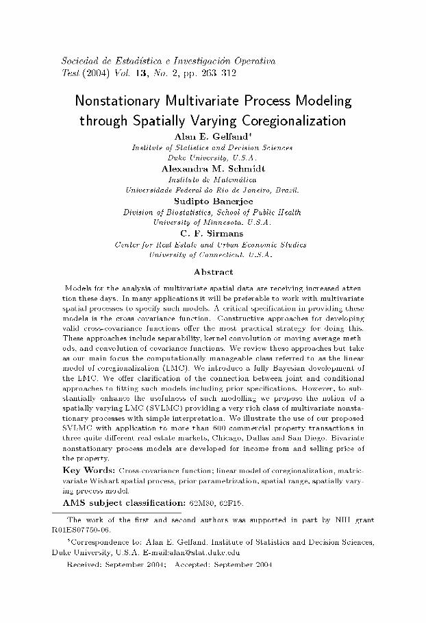
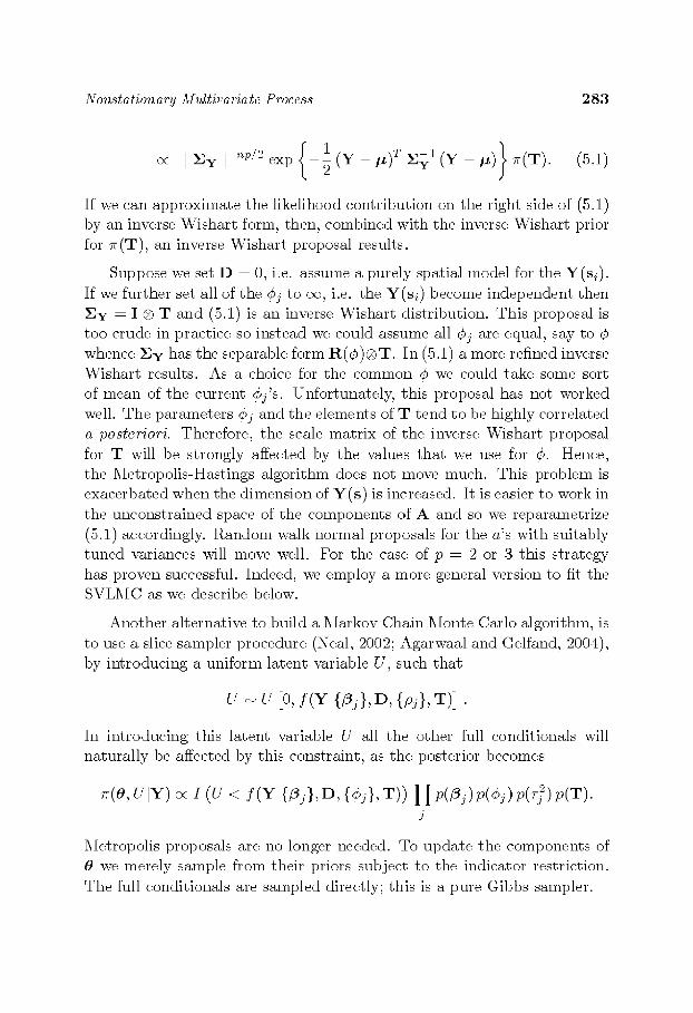
V~ consider a dataset consisting of apar tment buildings in three very distinct markets, Chicago, Dallas, and San Diego. The data were purchased from the CoStar Croup, Inc. (w~r~. c o s t a r g r o u p , corn). We have 252 build- ings in Chicago, 177 in Dallas, and 224 in San Diego. In each market, 20 additional transactions are held out for prediction of the selling price. The locations of the buildings in each market are sho~u~ in Figure 1. Note tha t the locations are very irregularly spaced across the respective markets. In fact, the locations were reprojected using UTM projections to correct for the difference in distance between a degree of latitude and a degree of longitude. All of the models noted below were then fitted using distance between locations in kilometers.
Our objective is to fit a joint model for selling price and net income and obtain a spatial surface associated with the risk, which, for any building, is given by net income/price. For this purpose we fit a model using the follow, Jag covariates: average square feet of a utfit within the building (sqft), the age of the building (age) and number of units ~ t h i n the building (unit)
286 A. E. Ge/fand, A. M. Schmidt, S. Baner]ee and C. F. Sirrnans
_ d
Chicago Dallas
- %
=
-88' 2
= .
�9 . == =- - ~ == =
= =
-88' ~ -87' 8 -87' 6
Longitude
a
0
- 1 1 7 4
e ! , . - a g.
0 c,
-E ca
oq ~
= -"
i - "'" ~ : = , . a -
i =
-97' 4 - 97 2
San Diego
=
1 ~ ' i o
= ~
|
- I 1 7 3 - I 1 7 2 - 1 1 7 1 - I 1 7 0 - I 1 6 9
Longitude
a =
o;
=
-" 2>
= ~ , ! ~ .
= a =
-~ ~ -9~ 8 -9~ 6
Longitude
F/gm'e 1: Sa.nlpling loca.tions fol" the thl'ee nial'kets in Chicago. Da.Ila.s a.nd San Diego.
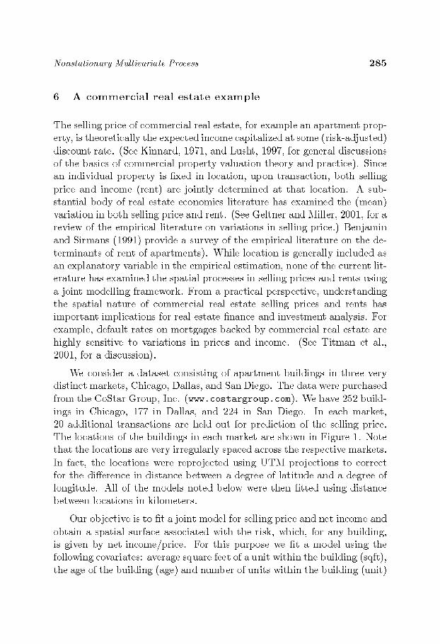
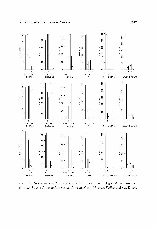
and the array. As is customary, we work with the logselling price of the transaction (P) and the lognet income (I). Figure 2 shows the histograms of these ve~riables. Note tha t they vary considerably across markets. The model is
I(s) sqa(s)..~,~ + age(~)..~,2 + u,~t(~).&3 + v~ (~) + q (~) (0.1)
Nonstatfonary Multivariate Process 2 8 7
o
N ~
nlt~ ~ unit
~ ~ N N
o
. 0 . (?
n ts Square II per unit
o
I I I I I
. . 0 2 .
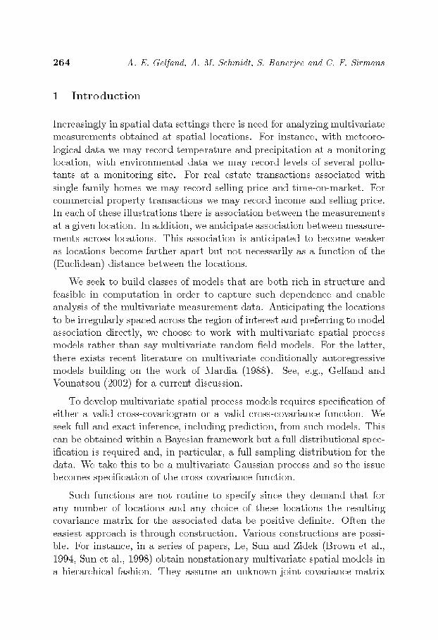
log Price log Incor'e log risk Age Number of Units Square It per unit
Figts'e 2: Histogra.ms of the ~,a.ria.bles log Price. log Income. lug Risk. age, number
of units. Squa.re ft per unit fur ea.ch of the ma.rkets. Chicago. Dalla.s and San Diego.
288 A. E. Gelfand, A. M. Schmidt, S. Banerjee and C. F. Sirrnans
I I C h i c a g o D a l l a s San Diego
M o d e l G P D G P D G P D
M o d e l 1 0.179;3 0 .7299 0.9092 0 .1126 0.51:38 0.62,64 0 .0886 0 .4842 0 .5728
M o d e l 2 0.1772 0 .6416 0 .8188 0 .0709 0 .4767 0 .5476 0.08;39 0 .4478 0 .5317
M o d e l ;3 0.1794 0.6;368 0.8162 0 .0715 0 .4798 0 .5513 0 .0802 0 .4513 0 .5315
M o d e l 4 0.1574 0 .6928 0.8497 0 .0486 0.498.5 0..5421 0.071;3 0 .4588 0.5:301
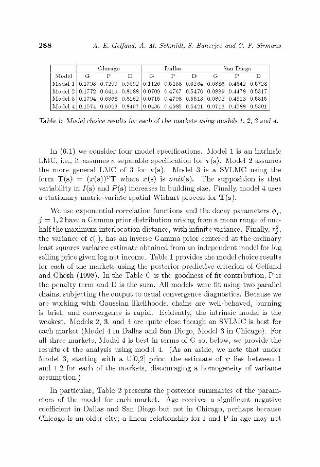
Table 1: %,Iodel choice resuIts for each of the markets using models 1, 2, 3 and 4,
In (6.1) we consider four model specifications. Model 1 is an intrinsic LMC, i.e., it assumes a separable specification for v(s) . Model 2 assumes the more general LMC of 3 for v(s). ikiodel 3 is a SVLMC using the form T(s ) = (a:(s))~"T where a:(s) is a n i t ( @ The supposit ion is tha t variability in I(s) and P ( s ) increases in building size. Finally, model 4 uses a s tat ionary matric-variate spatial Wishart process for T(s) .
Vv'e use exponential correlation functions and the decay parameters Oj, j = 1, 2 have a Gamma prior distribution arising from a mean range of one- half the maximum interlocation distance, with infinite variance. Finally, r~,
the variance of e(.), has an inverse Gamma prior centered at the ordinary least squares variance estimate obtained from an independent model for log
selling price given log ne~ income. Table 1 prox4des ~he model choice results for each of the markets using the posterior predictive criterion of Gelfand and Ghosh (1998). In the Table g is the goodness of fit contribution, P is the penalty term and D is the sum. All models were fit using two parallel chains, subjecting the output to usual convergence diagnostics. Because we are working with Gaussian likelihoods, chains are well-behaved, burning is brief, and convergence is rapid. Evidently, the intrinsic model is the weakest. Models 2, 3, and 4 are quite close though an SVLMC is best for
each market (Model 4 in Dallas and San Diego, Model 3 in Chicago). For all three markets, Model 4 is best in terms of g so, below, we provide the results of the analysis using model 4. (As an aside, we note that under Model 3, starting with a U[0,2] prior, the est imate of ~/, lies between 1 and 1.2 for each of the markets, discouraging a homogeneity of variance assumption.)
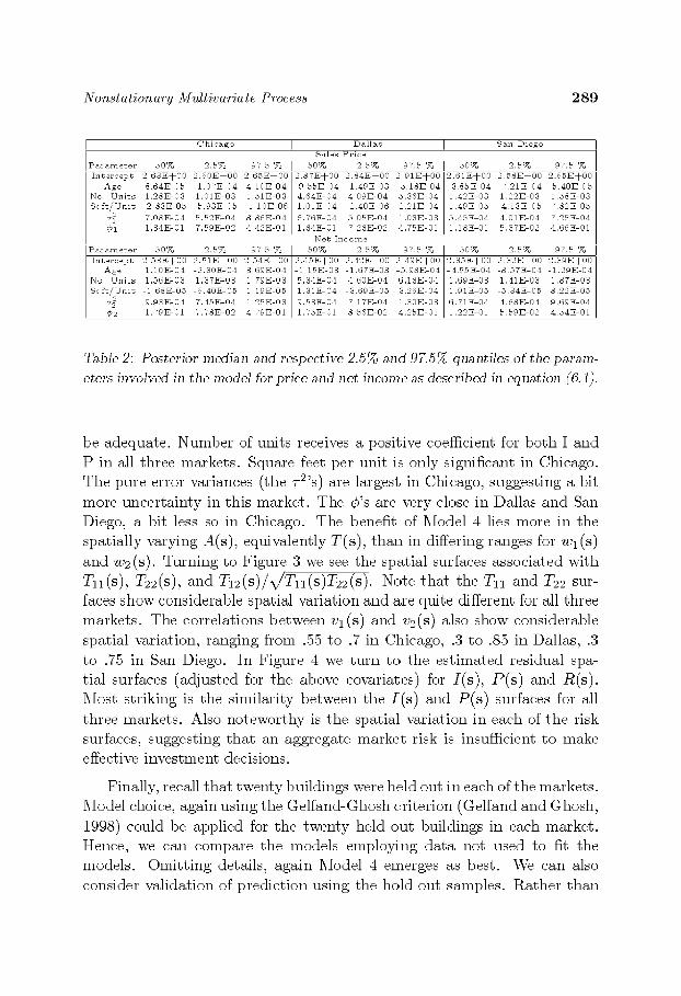
In particular, Table 2 presents the posterior summaries of the param- eters of the model for each nmrket. Age receives a significant negative coefficient in Dallas and San Diego but not in Chicago, perhaps because Chicago is an older city; a linear relationship for I and P in age may not
Nonstationary Multivariate Process 289
I I (-'. hic ~go I D ~ l l ~ s I S~n D i e g o S~les P r'ice
5OCTu 2 5 % 97.5 % 5OCTu 2.5c7u 97.5 % 5OCTu 2.5c7u 97.5 % I n t e r c e p t 2 6 3 E J - O O 2.6O]EJ-00 2 6 ~ E J - O O 2.871EJ-OO 2.841EJ-00 2 9J. EJ-OO 2.611EJ-00 2 ~8EJ-OO 2.6~EJ-OO
A g e 8.641E 05 1.071E 04 4 1 0 E 0 4 9 5 5 E 04 1 . 4 9 E 03 5 1 8 E 0 4 3.851E 04 7 . 2 1 E 04 5 4 0 E 05 N o U n i t s 1.28]{-03 1 .01E.-03 1 5 1 E - 0 S 4 .64]{-04 4 0 9 E - 0 4 5 . 3 6 E - 0 4 1.42]{.-03 1 2 2 E - 0 3 1.58]{-03 S q f t / U n i t 2 8 3 E 0 5 5.93]E 05 1 1 0 E 0 6 1.0lIE 04 2 . 4 0 E 06 2 . 2 1 E 04 1 . 4 9 E 05 4 . 1 3 E 05 7.82]E 05
w 1 7.081E 04 5 . 5 2 E 04 8 8 6 E 0 4 6.761E 04 5 0 5 E 04 1 . 0 3 E 03 5 . 4 5 E 04 4 0 1 E 04 7.251E 04 r 1 , 8 4 E - 0 1 7 ,59E.-02 4 , 4 2 E - 0 1 1,84]E-01 7 , 2 8 E - 0 2 4 , 7 5 E - 0 1 1,18]E.-Ol 5 , 8 7 E - 0 2 4.,~,~,E-01
N e t I n c o m e Pazameter 5 0 ~ 255~ 97.5 5~ 50~ 2 .5~ 97.5 5~ 50~ 2 .5~ 97.5 5~ I n t e z c e p t 2 5 3 E + 0 0 2.51]{.@00 2 5 4 E @ 0 0 2.45]{.+00 2 . 4 2 E @ 0 0 2 4 9 E + 0 0 2 . 8 5 E + 0 0 2 3 2 E @ 0 0 2 . 3 9 E + 0 0
A g e 1.10]E 04 2 . S 0 E 04 3 6 9 E 0 4 l l S E 03 1.67]E 03 5 9 8 E 0 4 4.55]E 04 8.57]E 04 1 2 9 E 0 4 No, Unit,~ 1,50]E-08 1,87]~-08 1 ,79G-08 b,34]E-04 4 , 0 0 E - 0 4 0 , 1 8 E - 0 4 1,~,9]~-08 1 , 4 1 E - 0 8 1,87]E-08 S q f t / U n i t - 1 6 8 E - 0 5 -o .40]{-05 1 1 9 E - 0 5 1 .31]{-04 -3.O9]E-05 3 . 2 6 E - 0 4 1 . 9 1 E - 0 5 - 5 . 3 4 E - 0 5 8 .22]{-05
~ 9 .93]{-04 7 . 4 5 E - 0 4 1 2 5 E - 0 3 9 .53]{-04 7 1 7 E - 0 4 1 . 3 0 E - 0 S 6 . 7 1 E - 0 4 4 6 8 E - 0 4 9 .o9]{-04 ~2 1.79]E 01 7.78]E 02 4 7 9 E 01 1.75]E 01 8 5 6 E 02 4 . 2 5 E 01 1.22]E 01 5 5 9 E 02 &.54]E 01
Table 2: Posterior media.n a.nd respective 2.5% and 97.5% quantiles of the pa.ra.m- eters involved in the model for price and net income as described in equation (6.1).
be adequate. Number of uuits receives a positive coefficient for both I and P in all three markets. Square feet per refit is only significant in Chicago. The pure error variances (the r2's) are largest in Chicago, suggesting a hit
more uncertainty in this market. The ~'s are very close in Dallas and San Diego, a bit less so in Chicago. The benefit of Model 4 lies more in the spatially varying A(s), equivalently T(s), than in differing ranges for w 1 (s)
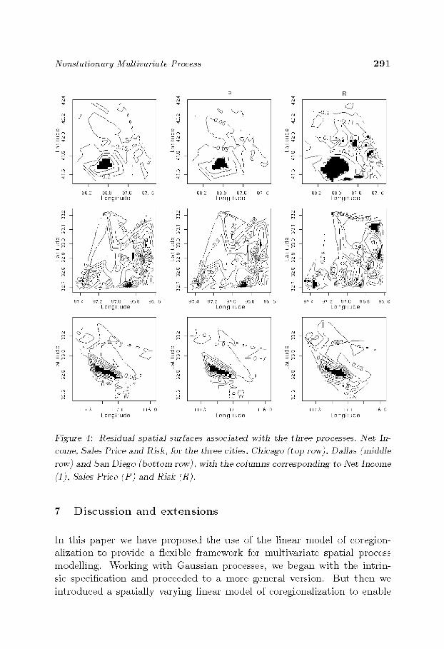
and w2 (s). Turning to Figure 3 we see the spatial surfaces associated with T~(s), T..(s), and T~.(s)/x/Tn(s)T:2(s ). Note that the Tn and T.. sur- faces show considerable spatial variation and are quite different for all three markets. The correlations between vl (s) and v2(s) also show considerable spatial variation, ranging from .55 to .7 in Chicago, .3 to .85 in Dallas, .3 to .75 in San Diego. In Figure 4 we turn to the est imated residual spa- tial surfaces (adjusted for the above covariates) for I(s) , P ( s ) and R(s). Most striking is the similarity between the I ( s ) and P ( s ) surfaces for all
three markets. Also noteworthy is the spatial variation in each of the risk surfaces, suggesting that an aggregate market risk is insufficient to make effective investment decisions.
Finally, recall tha t twenty buildings were held out in each of the markets. Model choic% again using the Gelfand-Ghosh criterion (Gelfand and Ghosh,
1998) could be applied for the twenty held out buildings in each market. Hence, we can compare the models employing da ta not used to fit the models. Omitt ing details, again Model 4 emerges as best. We can also consider validation of prediction using the hold out samples. Rather than

2 9 0 A. E. Gelfand, A. M. Schmidt, S. Baner3ee and C. F. Sirrnans
~q
;I
T1 l ( s ) T Z Z ( s ) T c o r r ( s )
i i i i
138.2 BBO BTB 137. 6 L o n g i t u d e
i i i i
974 972 97.0 96.13 96. L o n g i t u d e
I I I I
1173 1171 116 O L o n g i t u d e
ca
813.2 BBO B7.13 137. 6 L o n g i t u d e
x:Jm
974 97.2 97.0 96B 96 L o n g i t u d e
l l 7 3 l l 7 l L o n g i t u d e
/
I
118 9
m o
m
~q
m
i i i i
138.2 8130 87.13 137 6 L o n g i t u d e
i i i i
97.4 97.2 970 96B 96. L o n g i t u d e
I I I I I
1175 1171 116 o L o n g i t u d e
Figts'e 3: Spatial surfa.ces associated with the spatiaIly varying T(s) for the three cities, Chicago (top row), Dallas (,,fiddle rosy) and San Diego (bottom row), with the colu,,ms correspo,~di,~g to T:~ (s), T:2 (s) a,~d %o~ (s).
detailing all of the predictive intervals for each I and P in each market, we summarize by noting that for P, in Chicago 18 of 20 9.5% predictive intervals contained the observed value, 20/20 in Dallas and 20/20 in San Diego. For I, we have 19/20 in each market. It appears that Model 4 is providing claimed predictive performance.
Nonstationary Multivariate Process 291
o )
o ) o
~3
m
~S
I P R 2
o )
. % �9 ( ~ 0 . 0 G
i i i i i i i i
88 2 88 0 87 8 87 6 88 2 88 o 87 8 87 6 L o n g i t u d e L o n g i t u d e
o o
~3 c~
i i i i i i i i
974 97.2 97.0 95B 95 5 97.4 97.2 970 95B 96. 5 L o n g i H 4 d e L 0 n g i t u d e
i i i i
117 3 117 1 115 LongiH4de
m i : so
I I I I
1173 1171 116 9 Longitude
~3 c~
m
88 2 88 0 87 8 87 5 L o n g i t u d e
i i i i
974 9 7 2 970 96.8 96. 6 L o n g i t u d e
I I I I
1173 l l T 1 l l 6 9 Longitude
Fi~,Ln'e 4: Residua.l spatia.l sm'fa.ces associated with the three processes, Wet h~-
come, Sales Price a.nd Risk, for the three cities, Chicago (top row), Da.llas (middle
row) a.nd San Diego (bottom rosy), with the columns corresponding to Net Income
(t), Sa.los Price (P) a.,,d Risk (R).
7 D i s c u s s i o n a n d e x t e n s i o n s
In this paper we have proposed the use of the linear model of coregion- alization to provide a flexible framework for multix;ariate spatial process modelling. Working with Gaussian processes, we began with the intrin- sic specification and proceeded to a more general version. But then we introduced a spatially varying linear model of coregionalization to enable
292 A. E. Gelfand, A. M. Schmidt, S. Banerjee and C. F. Sirrnans
nonstat ionary multivariate spatial process models. Here we offered a ver- sion which allowed for heterogeneity to vary as a function of a covariate and then a more general version, introducing heterogeneity through a spatially varying Vs process.
Future effort will consider non Gaussian models for the data, e.g., ex- ponential family models for the components of Y(s ) . Dependence ~qll be introduced through components of a vector of spatially dependent random effects modeled as above. Also of interest are spatio-temp oral versions mod- eling v ( s , t ) A ( s , t ) w ( s , t ) where the components of w, w/(s , t ) are inde- pendent spatio-temporal processes. Depending upon the context, A(s , t) may be simplified to A(s) , A( t ) or A. Convetflent choices for the w,(s , t ) would be space-time separable specifications.
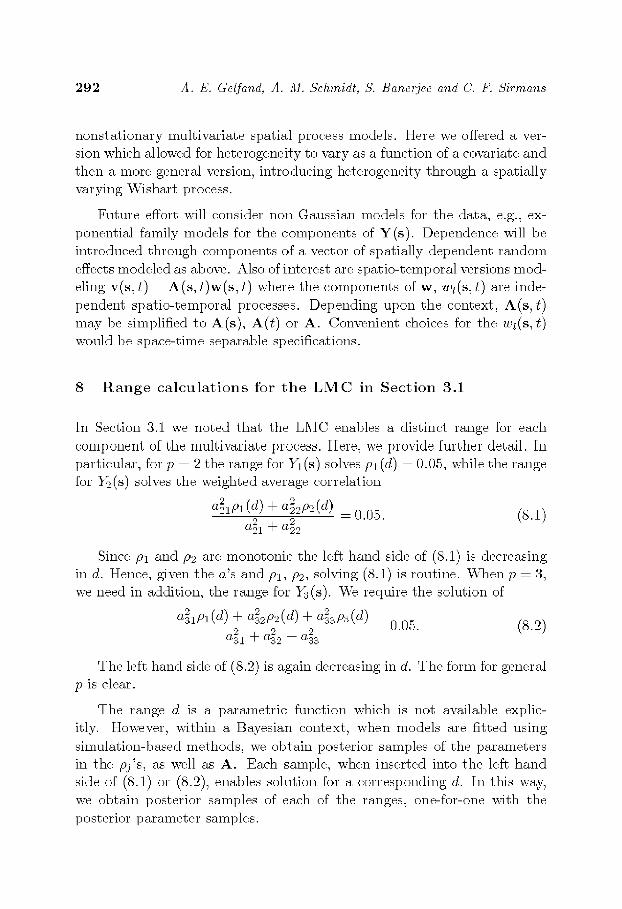
8 R a n g e c a l c u l a t i o n s for t h e L M C in S e c t i o n 3.1
In Section 3.1 we noted that the LMC enables a distinct range for each component of the nmltiv~riate process. Her% we provide further detail. In particular, for p 2 the range for Y~(s) solves p~(d) 0.05, while the range for Y2(s) solves the weighted average correlation
2 G e , (d)+ = O.OS. (8.1)
Since pl and p2 are monotonic the left hand side of (8.1) is decreasing in d. Hence, given the a's and Pl, P2, solving (8.1) is routine. When p 3, we need in addition, the range for ~ ( s ) . We require the solution of
+ Gp (d) + o.os. (s.2) + G +
The left hand side of (8.2) is again decreasing in d. The form for general /) is clear.
The range d is a parametric function which is not available explic- itly. However, ~i thin a Bayesian context, when models are fit ted using simulation-based methods, we obtain posterior samples of the parameters in the p f s , as well as A. Each sample, when inserted into the left hand side of (8.1) or (8.2), enables solution for a corresponding d. In this way, we obtain posterior samples of each of the ranges, one-for-one with the posterior parameter samples.
Nonstationary Multivariate Process 293
9 A l i g n i n g priors for u n c o n d i t i o n a l and cond i t i ona l process specif icat ions
Here we prove l, he result stated in Secl, ion 3.3. Again, we h a v e / ( T I A , v) oc
ITI ~+~+~ exp { } t r A T -1 }. Part i t ion T as T Tpp and zX as Tp 1,p ( A(p 1) 0 )
0 ZXp . Since v ( s ) ~ A'~(0, T), given ~'l(s), ...,~'~ l(s),
vp(s) ~ N(T~_I ,p(T@-I)) - Iv( p) ,Tpp- T~_I,p(T@-I))- ITp 1.p),
where v ~ (v l (~) , . . . , v~ 1(~). hence, using the notation of Section 3.2, C~p (T(p 1))1Tp_I,p and o-p 2 ~pp_ ~/_l,p(T(p 1))1Tp_I,p where
r (a~p) @) ' So, given T (p 1) the mapping from (Tp_l,p, Tpp) to O~p . , . . . ,Ctp 1}" (ctp, cr~) has Jgcobian IT+-1) I.
Standard results (see e.g. Harville, 1997, Section 8.5) yield ITI -- ~ Ir (p 1) I and
T 1 = T(p 1)+ T 2 __Otp/O-2 - ~ / ~ 1 / ~ �9
Making the change of variable,
we immediately have tha t cr~ .~ IG@/2 , As/2) and given cry,
,~ ~ n (0 ,~ (A(~ 1)) 1).
e the (P) Moreover, since A(p-1) is diagonal, given ~r, a 5 are conditionally
independent with ct.i crp .
More importantly, we see tha t ( ~ , c~p) are independent of T (p-l). Pro- ceeding backwards, we have for each t, (~r~,c~l) is independent of T (l-1), I 2 , . . . , p and thus T 0) Tn cry, (Crg, C~2),..., (Crp2,C~p) are indepen- dent. Also, setting p 2 in the above calculation reveals tha t f (TO)) oc
IT(~)I"T* exp{_~_trA(D(T(1)) 1}, i.e. /(or 2) oc g2 @+* exp{-~-(A1/s~)}, i.e., ~ ~ : C ( " ~ 1, ~ ) . Hence the result is proved.
294 A. E. Gelfand, A. M. Schmidt, S. Banerjee and C. F. Sirrnans
10 A s s o c i a t i o n s t r u c t u r e for t h e spa t ia l W i s h a r t p r o c e s s
Here we develop the spatial association s t ructure for a general SI'Vp (7/, F F T, p~, , pp process First, let S(s) Z(~)Z~(~) What can we say about the association between S(s) and E(s ')? In fact, we t~ave tt~e following simple results:
cov(SZ (s), Sj j (s'))
co~,(sjj, (s ), s z , (s') )
cov(Zj (s), zk~., (s') )
= 2,~g(~ ~')
= ,/pj(s s ')pj,(s s'), j r
= O, if either j ~ k or j ' ~ k'.
So S(s) is SI~ p(tJ, I, P1, - . - , Pp) and is comprised of 2
lated processes.
To prove these results we note that .~.jj(s) = E[--~ Z~(s ) and ~:jj,(s) = E L ~ z , j (s)Z~j , (s) . So, c o ~ . ( S A ( s ) , S z ( s ' ) ) = ,.,co~,(z~j(s),Z~j(s')). But z(z~j(~)) 1 and
whence
E E(zfj(s)Z~j(s')lZlj(S')) Z 2 j ( s ' ) ( 1 - 192(s - s t ) Jr- 102(s - st)Zlj(S2 1)
1 + 2pf(~- ~')
Similar calculations yield the other results. Re turn ing to f t(s) we have a ( . ) E , r z , ( . ) ( r z , ( @ ~ so we can imitate the above calculations re- placing Z,(s) by Z,(s) = F(Z,(s) . It, particular, when F is diagonal we obtain cov(a.ij(s),f2jj(s')) 2 , ,FJ jp j ( s - s'), cov(f2jy(s),f2jj,(s')) ,~r ~. .F ~. .,pj (~ - ~')p~, (~ - ~'), j r j ' and ~o~'(~, (~), ~Z~.~,, (~')) 0 i f j r ~-
33 33
or j ' # k'.
Finally, note Chat we can not explicitly compute the association struc- ture of the associated inverse Wishar t spatial process. Tha t is, ft -~ (s) F I (Z(s )ZT(s ) ) -~F 1 and association calculations require working with z ~(~).
Nonstationary Multivariate Process 295
D I S C U S S I O N
M o n t s e r r a t F u e n t e s Statistics Department.
North Carolina State University, U.S.A.
I congratulate the authors for presenting a comprehensive Bayesian t rea tment to the problem of multivariate spatial process modelling and estimation. The authors introduce an extension of linear coregionalization models (LCM) to handle lack of stat ionari ty by allowing the LCM coeffi- cients to be space-dependent. Their formulation of the problem is clean, their parameterizat ion is natural, and their conditional and unconditional algorithms elegant.
I certainly agree that the Bayesian perspective on the coregionalization models is a natural way of xdewing this multivariate spatial modelling and est imation problem. Overall, my main concern about this paper is the lack of motivation and insight for the different frameworks presented. The the- ory is beautiful. But, it is not clear how useful or in what situations and under what assumptions about the nature of the underlying spatial pro- cesses, one should implement the multivariate approaches presented here. Furthermore, very often in multivariate spatial problems, the main objec- tive is prediction rather than estimation. It is not clear if the multivariate
framework presented here would perform better for prediction than just a simple separable model or the traditional LCM. The application in the paper focuses on estimation, and there are not clear comparisons between models in terms of prediction.
My specific comments are of two types: First, regarding the extensions
of kernel-based nonstat ionary models to a multivariate case, and secondly regarding the application presented in the paper.
The multivariate version presented by the authors of the kernel- convolution nonstat ionary approach (Vet Hoef and Barry, 1998; Higdon et al., 1999), assumes that all the spatial processes ~ for I 1 , . . . , p , are generated by the same underlying w process. This is very restrictive, not so nmch in terms of explaining the spatial s tructure of the different
2 9 6 M. Fuer~tes
Y/ processes, since the kernel can be different for each process. However, the problem is tha t this multivariate model imposes a strong dependency between all the Yl processes, since all of them are generated by the same underlying cv process. Can this approach handle scenarios in which the Y,
are spatial processes, ~ i th spatial dependency-, but some of them are un- correlated with each other (or ahnost uncorrelated)? I am also concerned about the multivariate extension introduced by the authors of the convolu- tion approach of Fuentes (2001, 2002b,a) and Fuentes and Smith (2001), to handle nonstat ionari ty by representing the process in terms of local station- ary processes. In this case it is unrealistic to assume tha t each Y/ spatial process can be represented in terms of the same {Wo(0} t underlying local s tat ionary processes. These underlying {w0(t)}t processes determine the subregions of local stationarity. Thus, it is too restrictive to assume that all Y/ processes have the same underlying local s tat ionary behavior. It is true that the weights b, can be different for each Y/, but in this model the
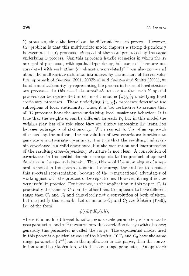
weights play less of a role since they are simply smoothing the transition between subregions of stationarity. Wi th respect to the other approach discussed by the authors, the convolution of two covariance functions to generate a multivariate covariance, it is true tha t the resulting multivari- ate covariance is a valid covariance, but the motivation and interpretat ion of the resulting cross-dependency structure is not clear. A convolution of covariances in the spatial domain corresponds to the product of spectral densities in the spectral domain. Thus, this would be an analogue of a sep- arable model in the spectral domain. I encourage the authors to consider this spectral representation, because of the computat ional advantages of working just with the product of two spectrmns. However, it might not be very useful in practice. For instance, in the application in this paper, C1 is practically the same as C2; on the other hand C~2 appears to have different range than C1 and C2 and thus clearly not a convolution of both of them. Let me justify this remark. Let us assume C~ and C2 are Ma%rn (1986), i.e. of the form
~(a-h)~K~(ah),
where K a modified Bessel function, 6 is a scale parameter, 1/is a smooth- ness parameter, and a -~ measures how the correlation decays wRh distance; generally this parameter is called the ra~.ge. The exponential model used in this paper is a particular case of the l~[a%rn. If C1 and C2 have the same range parameter ( a - l ) , as in the application in tixis paper, then the convo- lution would be l~iat~,rn too, with the same range parameter. An approach
Nonstationary Multivariate Process 297
like this one would be quite unrealistic in many settings.
This type of interpretation of the different proposed multivariate models is missing in the paper, and it would have been very helpful to gain some more insight and motivation about the proposed multivariate modeling frameworks.
A more flexible fl'amework could be achieved by writing the multivariate spatial process as
v(s) = a w ( s ) ,
with w(s ) - ( w l ( s ) , . . . , wp(s)), and treating each wi(s) for i - 1 , . . . , p , not as a s tat ionary process as the authors do, but as a nonstat ionary random field modeled using a kernel-based nonstat ionary covariance function (e.g. Higdon, 1998, Fuentes, 2002a). This might be easier to handle and imple- ment in practice than allowing the A components to change with space, as proposed by the authors to handle the lack of stat ionarity of v.
In terms of the application, it would have been helpful to clearly deter- mine the meaning of "estimated" parameter (e.g., the t..', parameter) and "estimated" residual spatial surfaces. I assume that refers to the mean, me- dian or mode of the posterior density or of the predictive posterior density. It is also important to discuss and interpret carefully the relevant parame- ter % tha t determines if the spatially varying version of the LCM approach presented by the authors is needed or not. The posterior distr ibution for this parameter, or some indication about the uncertainty associated to it, is needed to make this type of inference. If g, is not sigmficantly different from zero, then the proposed spatially varying coregionalization model reduces
to the LCM (with a s tat ionary covariance).
The authors present a calibration analysis to s tudy the performance in terms of prediction of the most complex model presented in the paper, with T(s ) = a ( s ) a ( s y modeled as a spatial process with an inverse Wishart distribution. However, it is not clear if a simple approach (LCM) would perform as well as this complex model. Calibration and/or cross-validation analysis to evaluate the perfornmnce in terms of prediction of the LCM are not presented. Therefore, the need and the advantages in terms of prediction of using these more complex models is not clear. The same comment applies to estimation. A criterion is presented to compare models. However, a clear gain in terms of esl, imation by using the most complex models is not evident, and the results could be different using a different
2 9 8 D. Hig don
criterion. Maybe a simulation s tudy or using other criteria (e.g. BIC) would help to make more clear the need for these models.
In view of the authors ' intention to implement their multivariate model in a space-time setting, I encourage them to consider the space-time ex- tension of LCM provided by De Iaco et al. (2003), using marginal semi- variograms. A Bayesian framework for De Iaco's approach could be a nice contribution to the space-time multivariate modeling literature.
D a v e H i g d o n Los Alam.os National Laboratory, U.S.A.
Thanks to the authors for an interesting paper on a difficult and im- por tant topic. The difficulty of this modeling effort is apparent in the fact tha t the invention of an inverse Wishart spatial process was required. The
use of nonstat ionary models is particularly appealing in the multivariate setting where the dependencies between spatial fields cannot be expected to be constant over large spatial domains.
R e l a t i o n t o o t h e r n o n - s t a t i o n a r y m o d e l s
It 's worth pointing out tha t particular variants of the SVLMC formula- tion will yield something very close to the non-stat ionary models of Higdon et al. (1999) and Fuentes and Smith (2001). I'll describe a very simple univariate example over a two-dimensional space. Take wl (s) to be a ge- ometrically anisotropic Gaussian process M t h strong dependence in the East-V~:est (E-W) direction; take w2(s) to be an geometrically anisotropic Gaussian process with strong dependence in the NNW-SSE direction; take
wa (s) to be an geometrically anisotropic Gaussian process with strong de- pendence in the NNE-SSW direction. Wi th these three "basis" processes, almost any direction of maximal dependence can be specified by taking the appropriate mixture. Here the univariate surface v(s) is modeled according to
where c(s) is a white noise process. One could specify the processes
(4,
Nonstationary Multivariate Process 2 9 9
to be dependent as in Higdon (1998) where each we(s) depends on a com- mon white noise process ~(s)
f t) (t)dt, e 1,...,a.
Alternatively, Fuentes and Smith (2001) specify the we(s)'s 1,o be indepen- dent of one another.
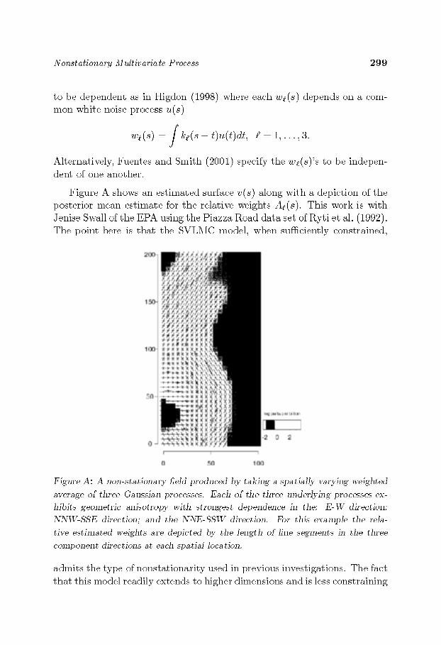
Figure A shows an est imated surface v(s) along with a depiction of the posterior mean estimate for the relative weights Ae(s). This work is ~ i th Jenise Swall of the EPA using the Piazza Road data se~ of RyCi e~ al. (1992). The point here is tha t the SVLMC model, when sufl%iently constrained,
I I
O 50
ItN [Jarle. [J ar bi li~1
II -2 0 2
I
10Q
Figm'e A: A non-sta.tionmT fidd produced by taking a. spa.tially var)~ng weighted
a.vera.ge of three Ga.ussia.n processes. Each of the three underlying processes ex- hibits geometric a~2isotropy with strongest dependence in the; E - W direction;
~,\~\qIuSSE direction; a.nd the . \WE-SSW direction. For this exa.mple the rela-
tive estfma.ted ~veights a.re depicted by the length of line segments in the three
component directions a.t ea.ch spa.tiaJ location.
admits the type of nonstat ionari ty used in previous investigations. The fact tha t this model readily extends to higher dimensions and is less constraining
300 D. Hig don
than previous nonstat ionary approaches is encouraging and suggests such a modelling specification may find use in a broad base of applications.
S m o o t h n e s s
In thinking about constructing nonstettionary spatial models I have always had in mind a decomposit ion of the spatial field into a smooth piece with appreciable spatial dependence plus a rough piece with a very limited range spatial dependence (often, a white noise model is sufficient for this rough component) . I've focused on imparting the nonstat ionary modeling into the smooth component of the field. Hence I've been happy to consider very smooth processes even though I may not expect the actual spatial field to exhibit such smoothness. I suspect this means I 'm predisposed to using very smooth specifications for latent model components which control nonstationarity. This predisposition can lead to lower dimensional models which can simplify computing, but I know of no general principles here.
In contrast, the authors allow a fair bit of local spatial variation in the inverse Wishart spatial process by using an exponential correlation function to control the dependence in the pTe independent gauss ian processes models from which the spatial process is constructed. Hence T(s) and T(s + d ) - with 5 small - will be far less similar when the underlying spatial correlation functions are exponential as compared to Gaussian. To get an idea of the difference between these two alternatives, Figure B shows the process of constructing a component of the SVLMC model v~ (s) when the exponential correlation model is used for the spatial Wishar t process for T-~(s) :
,/ge(d , I / �9
p (d) e• 1,2.
The large value of lJ is used to make the distr ibution less diffuse as it
would be in the posterior. Figure C shows analogous realizations for the case where T(s) is constructed from smoother Gaussian process realizations which are governed by a gauss ian covariance function pc(d) e x p { - (4d)2}. In both figures, the resulting surface v~(s) is constructed from a linear combination of two smooth processes w~ (s) and w2(s).
A potential difficulty with the rougher inverse spatial Wishart process of Figure B is tha t it doesn ' t allow a smooth vA~(s) field. If snmll scale
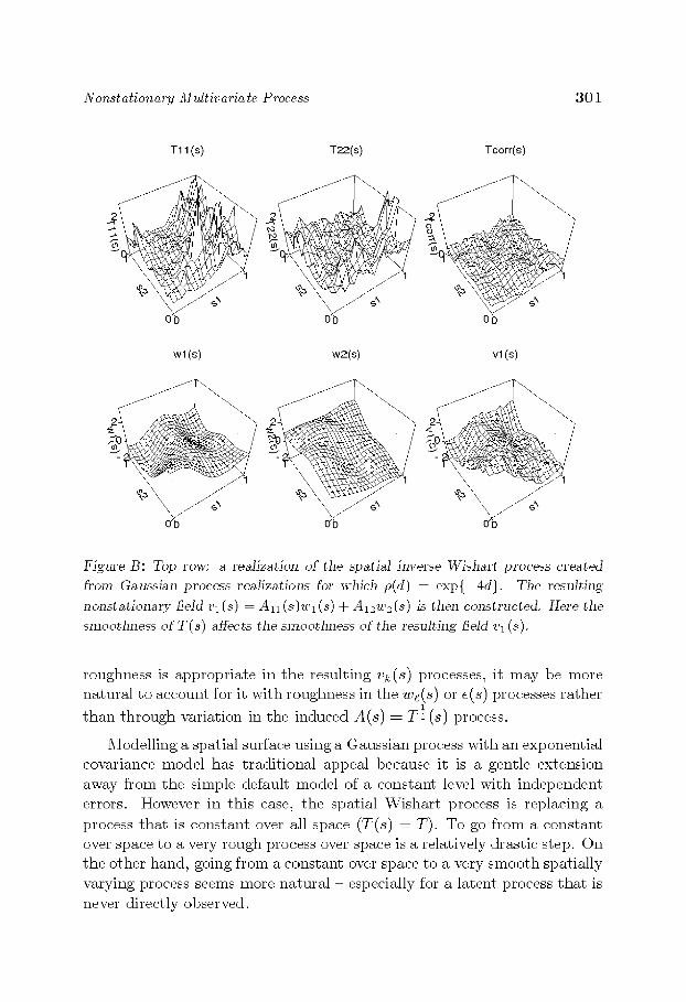
Nonstationary Multivariate Process 301
T11 (s) T22(s) Tcorr(s)
. .L
wl (s) w2(s) vl (s)
Figm'e B: Top row: a realization of the spa.tial fnverse I.t.Tshart process crea.ted
nonsta.tiona.ry field v: (s) - A ~ (.s-)w~ (s) + A~awa (.s-) is then constructed, Here the
smoothness of T(s) affects the smoothness of the resulting field v: (s).
roughness is a pp rop r i a t e in the resul t ing vk(s) processes, it may be more na tu ra l to accoun t for it wi th roughness in the we(s) or e(s) processes ra the r
t h a n t h r o u g h var ia t ion in the induced A ( s ) = T ~ ( s ) process.
Model l ing a spatial surface using a Gauss ian process wi th an exponen t ia l
covar iance model has t r ad i t iona l appea l because it is a gent le ex tens ion
away f rom the simple defaul t model of a cons tan t level wi th i ndependen t
errors. However in this case, the spat ia l W ish a r t process is replac ing a
process t h a t is cons t an t over all space (T(s ) = T) . To go f rom a cons tan t over space to a very rough process over space is a re la t ively dras t ic step. On
the o the r hand , going f rom a cons tan t over space to a very s m o o t h spat ia l ly
vary ing process seems more na tu ra l - especial ly for a la tent process t h a t is
never d i rec t ly observed.
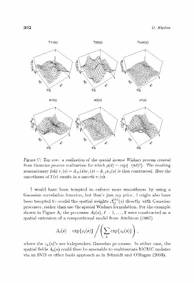
3 0 2 D. Higdon
T1 l(s) T22(s) Tcorr(s)
,....
g
wl (s) w2(s) v l (s)
Figm'e C: Top row: a realization of the spatia.l h~verse ~.Yishart process crea.ted
fi'om Ga.ussian process reaYzatfons for which p(d) -- exp{ (4d)2). The result ing
nonsta.tionary tidal ~': (s) - Az: (s)~': (s) + A:~'~(s) is then constructed. 1-1ere the
I would have been tempted to enforce more smoothness by using a Gaussian correlation function, but that 's just my prior. I might also have
been t empted to model the spatial weights A!. ~) (s) directly ~ t h Gaussian t . /
processes, rather than use the spatial Wishart formulation. For the example shown in Figure A, the processes A s ( s ) , f = 1 , . . . , 3 were constructed as a spatial extension of a compositional model from Aitchison (1987)
where the zk (s)'s are independent Gaussian processes. In either case, the spatial fields A s ( s ) could then be amenable to multivariate iXICiXIC updates via an SVD or other basis approach as in Schnfidt and O'Hagan (2003).
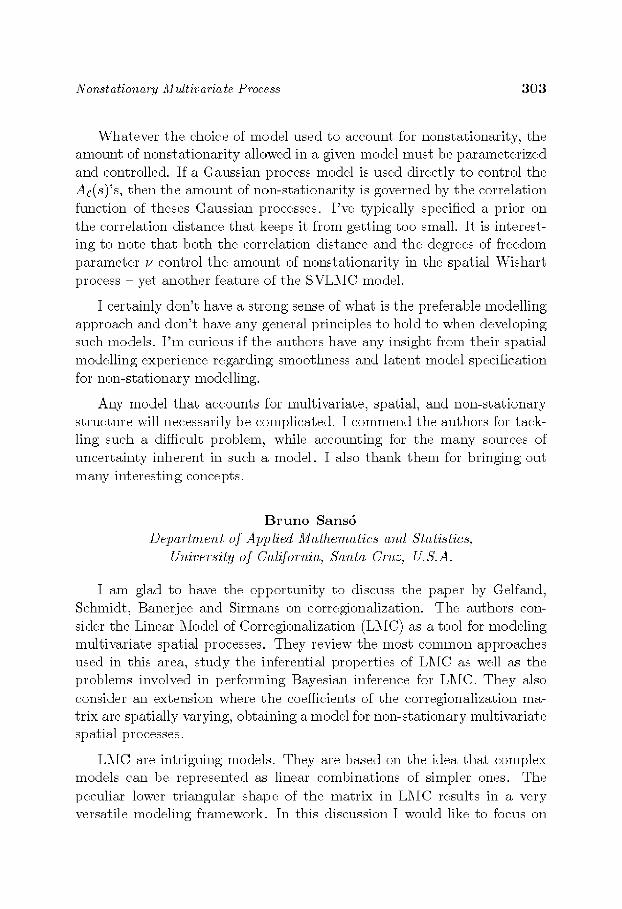
Nonstationary Multivariate Process 303
Whatever the choice of model used to account for nonstationarity, the amount of nonstat ionari ty allowed in a given model must be parameterized and controlled. If a Caussian process model is used directly to control the Ae(s)'s, then the amount of non-stat ionari ty is governed by the correlation
function of theses Gaussian processes. I've typically specified a prior on the correlation distance that keeps it from getting too small. It is interest- ing to note tha t both the correlation distance and the degrees of freedom parameter 7/control the amount of nonstat ionari ty in the spatial Wishart process - yet another feature of the SVLMC model.
I certainly don ' t have a strong sense of what is the preferable modelling approach and don' t have any general principles to hold to when developing such models. I 'm curious if the authors have any insight from their spatial modelling experience regarding smoothness and latent model specification for non-stat ionary modelling.
Any model that accounts for nmltivariate, spatial, and non-stat ionary structure will necessarily be complicated. I commend the authors for tack- ling such a difficult problem, while accounting for the many sources of uncertainty inherent in such a model. I also thank them for bringing out many interesting concepts.
B r u n o Sansd Department of Applied M~thematies and Statistics,
University of California, Santa Cruz, U.S.A.
I am glad to have the oppor tuni ty to discuss the paper by Gelfand, Schmidt, Banerjee and Sirmans on corregionalization. The authors con- sider the Linear Model of Corregionalization (LMC) as a tool for modeling multivariate spatial processes. They review the most common approaches used in this area, s tudy the inferential properties of LMC as well as the problems involved in performing Bayesian inference for LMC. They also consider an extension where the coefficients of the corregionalization ma- trix are spatially varying, obtaining a model for non-stat ionary multivariate spatial processes.
LMC are intriguing models. They are based on the idea that complex models can be represented as linear combinations of simpler ones. The peculiar lower triangular shape of the matrix in LMC results in a very versatile modeling framework. In this discussion I would like to focus on
304 B. Sansd
one of the extensions proposed in the last section of the paper, regarding spatio-temporal processes.
LIXIC can be used to consider mfivariate spatio-temporal models in t~D different ways. Vv'e can fix a location and stack the observations
obtained for all times in one vector per location. Or, we can fix t ime and stack spatial observation in one vector per time. iX[ore precisely, let ~/,(s) be a univariate process observed at times * = 1 , . . . , T and locations s = s~ , . . . , s , , . Then we can consider a LMC based on Yes) = Awes) where We can also consider a LIX C by assun ing
tha t Y t -- Awe, where Yt - (y , ( s l ) , . . . ,y , ( s , , . ) ) . In both ceases A ~ill be triangular matrices and w(s) and we suitable latent processes. These approaches are developed in Sans5 and Schmidt (2004) where the authors explore a whole range of possibilities with varying levels of sophistication.
An approach to multivariate space-time modeling tha t uses linear con>
binations of latent processes is presented in C~lder (2003). The work is based on the use of process convolutions embedded in a dynamic linear model (see, for example, V~.~st and Harrison, 1989). One of the devel-
opments in Calder's thesis is t ime-varying factor analysis for multivariate spatio-temporal random fields. This provides an exploration of the behav- ior of the most influential latent components. It would be interesting to know if the exploration of the latent process to of the LikIC can provide an alternative way of factoring the variability in the data.
To obtain a multivariate space-time model we can build a t ime varying extension of the LMC. One possibility is to consider a t ime varying matr ix
A, using methods developed in ~he literature for stochastic vol~ili~y (see, for example, Liu, 2000). Denote Ye(s) the multivariate process at t ime �9 and location .s. Then we assume tha t Ye(s) = Aew(.s). Let AeA', = ~ - 1 . We obtain a temporal structure by imposing a temporal evolution on e , . rol lo,~ng the results in Liu (2000), let L ( e t 1) denote the (lower triangular) Cholesky factor of flit 2- Then, for 0 < 8 <1 we define
g'e L(ffxe 2)H,L(g ' , 1)'/a where H , ~ B e p ( & z , 1 / 2 , ( 1 - a ) , z , 2/2).
Here B%(-,-) denotes a matr ix-beta distribution as defined, for exam- pie, in Muirhead (1982). a can be regarded as a discount factor for the evolution equation. Denote D, the information proxdded by the da ta up to time t. If we assume tha t p(~I'e_llD,_~) = I'Vv(rte_~, &_ l ) , a Wishart
Nonstationary Multivariate Process 305
distr ibution of dimension p • p and parameters he-1 and S t - l , then
; (<l>e 1)=%(a~, 1,~/ase 1).
Let Yt (Yt (s l ) , . . . , Y t ( s , , ) ) the p • n matr ix of observations. Then
Yt follows a matr ix-normal distr ibution (see, for example, V~:est and Harri- son, 1989), with row covariance matr ix ~Pe 1 and column cove~riance matr ix
R. Then
v(~lDe, R) ~ v(Vel~,,R)v(~eIDe 1) Im, l"/2exp{ t,-(v,~ 1v'e~,O/2 } • ~''~-~ -~-1)/2 exp{-t,-(as~11%)/2} I~t l (&'~-*+"-v-*) /2exp{- tr(6821 + YeR-*Y'e) ' .~e/2 }
n re) %(,~e, s,)
with .nt = 6.nt 1 + n and St = 5 S~11 + Y t R lyre. This provides a conjugate
evolution model for ~Pt, conditional on R. This conjugacy can be used to
simplify and possibly optimize iterative sampling methods. Since R is a
matr ix of spatial covariances it is cus tomary to consider a parameter ized
version, say R = R(A), where A is a low dimensional parameter .
An alternative model would be to consider ~Pt fixed in t ime and let Rt
vary in time. Under a Wishar t -Beta evolution, such model would produce
results similar to the one obtained above. Alternatively, if Re = R(At), we
can assume an evolution on At. This would be a more natural assumption, given the spatial nature of the covariances in Re, but it ~Jll eliminate the
conditional conjugacy. V~.~ notice tha t in either cases the models are assum-
ing tha t the spatial covariance s t ructure is common to all the components
of the random field. It would interesting to explore how tractable would be
a model where this assumption is dropped.
Rejo inder by A. E. Ge l fand , A. M. S c h m i d t , S. Baner jee and C. F. S i rmans
It is delightful to have had three knowledgeable, thoughtful and insight-
ful discussants comment on our contribution. Fuentes offers a demanding
306 A. E. Gelfand, A. M. Schmidt, S. Banerjee and C. F. Sirrnans
evaluation covering nmch territory, seeking a high standard, as she demands in her o~1 work. Higdon provides some lovely clar ifcat ion with regard to the inherent smoothness properties of our model specification. Sans6 fo- cuses on spatio-temporal extensions of our work, connecting to new work
he has just completed with one of us (Schnfidt). The discussants were gen- erous in their remarks, sett ing primary emphasis on comparison with other mechanisms for generating multivariate spatial models and on space-time versions of such models. In this rejoinder we ~11 confine ourselves to these t~D issues.
Before doing so, we note tha t we are not necessarily- advocating the use of coregionalization over, say, kernel methods to develop multivariate spatial process models. V~e are more concerned with trying to reveal tha t coregionalization can be viewed as a flexible, easily interpreted modeling tool rather than its customary use in the l i terature as a dimension reduction technique. We also feel tha t the spatially varying version offers a very rich, nonstat ionary class of specifications while again retaining ease of interpre- tat ion as well as computat ional tractability. V~e also note that our example and the associated analysis are primarily illustrative. V~'e believe that the modeling is appropriate for the price and income data we have collected on commercial real estate but readily acknowledge, as Fuentes observes, tha t our analysis is far from definitive. As for Higdon's point regarding modeling the components of A(s) through Gaussian processes rather than through the spatial Wishar t formulation, this was our natural starting point. In the end, we preferred the interpretation (particularly with regard to prior specification) tha t arises ~-ith A t s ) A t s ) T = r t s ) being marginally Wishart.
With regard to multivariate spatial process modeling using kernels, we were struck by the fact tha t the only readily-discovered work was that of Vet" Hoef and Barry (1998)and Vet' Hoef et al. (2004). In this work, a c o m - mon umvariate process is mixed to create all components of Y(s ) with the choice of kernel de termiNng the marginal process for each ~ ( s ) . So, exten- sions of the "Higdon" and the "Fuentes" approaches were presented in this spirit. But , Fuentes is correct in noting the limitations of such extension and she also makes the keen observation that , within the LMC, nonstation-
arity can be achieved by having the independent processes be nonstation- ary, rather than introducing a spatially varying A(s). Higdon is certainly correct in noting that the SVLMC formulation can well-approximate the nonstat ionary kernel approaches of both Higdon and Fuentes.
Nonstationary Multivariate Process 307
To remedy the limitations of a common univariate process in the case of the Higdon approach we can extend (6) (subsuming (2)) from out" paper to
Y(s) = . / K ( s t ; s ) v ( t ) d t
where K is a p • p diagonal matrix of kernel functions and v( t ) arises through a L),[C, i.e., v ( t ) Aw( t ) . By requiring p different kernels we may find it difficult to identify the parameters in the kl and also in A. If the kernel functions decrease very rapidly away from 0, the above model behaves like a LMC.
As a way to create a corresponding remedy for the Fuentes approach, we might return to the nested covariance model given in (13) of our paper. An integral version of (13) yields Y(s ) Since U is arbi trary we could let it be R 2 so tha t u indexes locations. In fact, we could write Y(s ) f A(t)wo(t)(s)dt. Continuing, if we replace A(t) with B(s; t) where B(s; t) is a p • p matrix of weight (inverse distance) functions, we obtain a different extension of the Fuentes model. This will become even more satisfying if we introduce both a weight matrix and intrinsic LI\IC's writing
r ~
Y(s) = j B(s;t)A(t)v(s,t)dt.
Hence, w0(t)(s) A ( t ) v ( s , t ) . In practice, we would use a finite sum approximation and might set B(s; t) = b(s; t) /p.
Turning to the space-time setting, when the the da ta takes the form Y(si, t) for locations s i , i 1, 2, ...,n and times t 1,2, ...T, then we can
concatenate the measurements over locations at t ime t to a vector Yt or we can concatenate the measurements over t ime at location si to a vector Y(si ) . This is the setting that Sansd considers and, in particular, the latter form naturally leads to a T-dimensional coregionalization model for Y(s) . The basic coregionalization model may be quite helpful here, allowing us to work ~_th T independent processes but the spatially varying version would introduce A as a T • T matrix and would yield a considerable increase in dimension as T grows large. The former suggests the possibility of core- gionalization using independent temporal models though a more natural formulation might lead to modeling through the use of a dynamic model where second stage random effects, say wt, are upda ted using random in- novations of a spatial process.
Arguably, the more interesting spatio-temporal extension would con- sider multivariate da ta at locations in space and in time, i.e., Y(s , t) where Y ' s are p • 1. This leads to the forms we suggested in our Section 7, i.e., we would write w(s , t) - Av(s , t) where the v's consist of p independent
308 A. E. Gelfand, A. M. Schmidt, S. Banerjee and C. F. Sirrnans
space-time processes. To add space, time, or space-time coregionalization we would introduce A(s), A(t) or A(s,t) , respectively. Modeling for the space time processes can be introduced using separable forms, the more general product-sum covariance specifications proposed in De Iaco et al. (2003) (as noted by Fuentes) or using nonseparable models as offered in e.g., Cressie and Huang (1999) or in Gneiting (2002). In fact, if time is viewed as discrete, then we might again employ a dynamic model, now introducing multivariate second stage spatial random effects, evolving through inde- pendent innovations of a multivariate spatial process. An illustration was provided in Gelfand et al. (2004).
R e f e r e n c e s
AGARWAAL, D. and GELFAND, A. E. (2004). Slice Gibbs sampling for simulation based fitting of spatial data models. Statistics and Computing. To appear.
AITCHISON, J. (1987). The Statistical Analysis of Compositional Data. Chapman & Hall, London.
BANERJEE, S., CARLIN, B. P., and GELFAND, A. E. (2004). Hierarchical Modeling and Analysis for Spatial Data. Chapman-Hall CRC Press, Boca Raton.
BANERJEE, S. and GELFAND, A. E. (2002). Prediction, interpolation and regression for spatial misaligned data points. Sankhya, 64:227-245.
BENJAMIN, J. and SIRMANS, G. S. (1991). Determinants of apartment rent. Journal of Real Estate Research, 6:357 379.
BERLINER, L. M. (2000). Hierarchical bayesian modeling in the environ- mental sciences. Allgerneine Statistiche Archly (Journal of the German Statistical Society), 84:141-153.
Box, S. E. P. and TIAO, S. C. (1992). Bayesian l~f~rence in Statistical Analysis. John Wiley ~nd Sons, New York.
BROWN, P. J., LE, N. D., and ZIDEK, J. V. (1994). Multivariate spatial hlterpolation and exposure to air pollutants. The C~nadian ,]ourn~d of Statistics, 22(4):489 509.
Nonstationary Multivariate Process 309
BROWNE, W., DRAPER, D., and GOLDSTEIN, H. (2002). Bayesian and likelihood methods for fitting multilevel models with complex level-1 vari- ation. Computatio~al Statistics a~d Data Analysis. To appear.
CALDER, C. A. (2003). Ezploring Latent Structure in Spatial Temporal Processes Using Process Convolutions. Ph.D. thesis, Institute of Statis- tics and Decision Sciences, Duke Umversity, Durham, North Carolina, USA.
CRESSIE, N. A. C. and HUANG, H. C. (1999). Classes of nonseparable spatio-temporal stationary covariance functions. Journal of th.e America~ Statistical Association, 94:1330 1340.
DE IAC;O, S., MYERs, D. E., and POSA, D. (2003). The linear coregional- ization model and the product-sum space-time variogram. Math.em.atical Geology, 35(14):25 38.
FUENTES, M. (2001). A new high frequency kriging approach for nonsta- tionary environmental processes. Envirometrics, 12:469-483.
FUENTES, M. (2002a). Modeling and prediction of nonstationary spatial processes. Biometrika, 2:281 298.
FUENTES, M. (2002b). Spectral methods for nonstationary spatial pro- cesses. Biometrika, 89:197-210.
FUENTES, M. and SMITH, PL. L. (2001). A new class of nonstationary spatial models. Tech report, North Carolina State University, Raleigh.
GASPARI, G. and COHN, S. E. (1999). Construction of correlation func- tions in two and three dimensions. Quarterly Journal of th.e Royal Me- tereological Society, 125:723 757.
CELFAND, A. E., BANERJEE, S., and CAMERMAN, D. (2004). Spatial process modelling for univariate and multivariate dynanfic spatial data. Em~ironmetrics. Forthcoming.
GELFAND, A. E. and GHOSH, S. K. (1998). Model choice: A minimum posterior predictive loss approach. Biometrika, 85:1 11.
GELFAND, A. E. and VOUNATSOU~ P. (2002). Proper multivariate con- ditional autoregressive models for spatial data analysis. Biostatistics, 4:11 25.
310 A. E. Gelfand, A. M. Schmidt, S. Banerjee and C. F. 5'irrnans
GEL'TNER, D. and MILLER, N. G. (2001). Comm.ercial Real Estate Analysis and Investments. South-V~.)stern, Cincinnati.
GNEITING, T. (2002). Nonseparable, stationary covariance functions for space-time data. Journal of th.e American Statistical Association, 97:590 600.
GOTWAY, C. A. and HARTFORD, A. H. (1996). Geostatistical methods for incorporating auxiliary information in the prediction of spatial vari- ables. Journal of Agricultural, Biological, and Environmental Statistics, 1(1) :17-39.
GOULARD, M. and VOLXZ, M. (1992). Linear coregionalization model: Tools for estimation and choice of cross-variogram matrix. JlJath.em.atical Geology, 24:269 286.
GRZEBYK, M. and \u H. (1994). Multivariate analysis and spatial/ temporal scales: Real and complex models. In Proceedings of the XVIIth International Biometrics Co~@rence, pp. 19-33. Hamilton, Ontario.
HARVILLE, D. A. (1997). Matrix Algebra from. a Statistician's Perspective. Springer, New York.
HIGDON, D. (1998). A process-convolution approach to modeling tem- peratures in the North Atlantic Ocean. Journal of Environmental and Ecological Statistics, 5:173 190.
HIGDON, D., LEE., H., and HOLLOMAN, C. (2002). 5[arkov chain Monte Carlo based ap-proaches for inference in computational intensive prob- lems. In J. M. Bernardo and 3. O. Berger, ads., Bayesian Statistics Z Proceedings of the Seventh. �88 M~eting.
HIGDON, D., SWALL, J., and KERN, J. (1999). Non-stationary spatial modeling. In J. M. Bernardo and J. O. Berger, ads., Bayesia~ Statistics 6, Proceedings of the Sixth �88 Meeting, pp. 761 768.
KINNARD, W. N. (1971). Income Property Valuations. Lexington Press, Lexing~con, MA.
LIu, F. (2000). Bayesian Time Series: Analysis Methods Using Simulation Based Comput(ttion. Ph.D. thesis, Institute of Statistics and Decision Sciences, Duke University, Durham, North Carolina, USA.
Nonstationary Multivaria te Process 311
LUSH'r, K. M. (1997). Real Estate �88 Irwin, Chicago.
MAJUMDAR, A. and GELFAND, A. E. (2004). Multivariate spatial model- ing using convolved covariance functions. Tech report, Institute of Statis- tics and Decision Sciences, Duke University, USA. Submited.
MARDIA, K. V. (1988). Multi-dimensional multivariate Gaussian Markov random fields ~ith application to image processing. ,Journal of Multi- vari~te Analysis, 24:265 284.
MARDIA, K. V. and GOODALL, C. R. (1993). Spatial-temporal analysis of multivariate emdromnental monitoring data. In G. P. Patil and C. R. Rao, eds., Multivariate Enviro~me~tal Statistics, pp. 347-386. Elsevier Science Publishers.
MATt~RN, B. (1986). @atial variation, vol. 36 of Lecture Notes i~ Statistics. Springer-Verlag, Berlin, 2nd ed.
MATHERON, G. (1982). Pour une analyse krigeante des donn~,es r~gionaligees. Tech report, Ecole Nationale Sup~rieure des Mines de Paris, Paris.
MUIRHEAD, P~. J. (1982). Aspects of Multivariate Statistica Theory. John Wiley and Sons, New York.
NEAL, i~. (2002). Slice sampling. A~znals of Statistics. To appear.
PACIOREK, C. J. and SCHERVISH, M. J. (2004). Nonstationary covariance functions for gaussian process regression. Advances in Neural I~iforma- tio~z Processing Systems, 16:1-8.
ROYLE, J. A. and BERLINER, L. M. (1999). A hierarchical approach to multivariate spatial modeling and prediction. Journal of Agricultural, Biological a~d Em~iro~mental Statistics, 4:29-56.
RYTI, 1%. T., NEPTUNE, B., and GROSKINSKY, B. (1992). Superfund soil cleanup: Applying the Piazza Road remediation plan. Environmental testing and Analysis, 1:26-31.
SANSd, B. and SCHMIDT, A. M. (2004). Spatio-temporal models based on discrete convolutions. Tech. Rep. ares2004-06, Department of Applied Mathematics and Statistics, University of California Santa Cruz.
312 A. E. Gelfand, A. M. 5'chmidt, S. Banerjee and C. F. 5'irrnans
SC;HMIDT, A. and GELFAND, A. E. (2003). A Bayesian coregionalization model for multivariate pollutant data. Yournal of Geophysics Research - Atmospheres, 108(D24):8783.
SCHMIDT, A. M. and O'HAGAN, A. (2003). Bayesian inference for non- stationary spatial covariance structure via spatial deformations. Yournal of the Royal Statistical Society, 65:745-758.
SPIEGELHALTER, D., THOMAS, A., BEST, N., and GILKS, W. (1996). Bugs 0.5 Bayesian inference using Gibbs sampling. Manual, version ii, 5IRC Biostatistics Unit, nstitute of Public Health, Cambridge, UK.
STEIN, M. L. (1999). Interpolation of Spatial Data. Springer-Verlag, New York.
SUN, W., LE, N. D., ZIDEK, J. V., and BURNETT, R. (1998). Assess- ment of a Bayesian muRivariate interpolation approach for health impact studies. Environmetrics, 9:565-586.
TITMAN, S., TOMPAIDIS, S., and TSYPLAKOV, S. (2001). Market imper- fections, investment optionality and default spreads. Technical report, University of Texas, Austin.
VARGAS-GUZMXN, J. A., \u A. W., and MYERS, D. (2002). Core- gionalization by linear combination of nonorthogonal components. M~th- ematical Geology, 84:405-419.
VER HOEF, J. M. and BARRY, t{. D. (1998). Constructing and fitting models for cokriging and multivariable spatial prediction. Journal of Statistical Planning and Inference, 69:275 294.
VER HOEF, J. M. C., C., N. A., and BARRY, R. P. (2004). Flexible spatial models based on the fast Fourier transform (FFT) for cokriging. .Journal of Computational and Graphical Statistics. To appear.
\u H. (2003). Multivariate Geostatistics - An Introduction with Applications. Springer-Verlag, New York, 3rd ed.
WEST, M. and HARRISON, J. (1989). Bayesian Forecasting and Dynamic Models. Springer Verlag, New York.