BAYESIAN STATISTICS 9,J. M. Bernardo, M. J. Bayarri, J. O. Berger, A. P. Dawid,D. Heckerman, A. F. M. Smith and M. West (Eds.)c! Oxford University Press, 2010

Nonparametric Bayesian Networks

Katja Ickstadt1, Bjorn Bornkamp1, Marco Grzegorczyk1, Jakob Wieczorek1

M. Rahuman Sheriff2, Hernan E. Grecco2 & Eli Zamir2

1TU Dortmund University, Germany2Max-Planck Institute of Molecular Physiology, Dortmund, Germany

ickstadt@statistik.tu-dortmund.de

Summary

A convenient way of modelling complex interactions is by employing graphsor networks which correspond to conditional independence structures in anunderlying statistical model. One main class of models in this regard areBayesian networks, which have the drawback of making parametric assump-tions. Bayesian nonparametric mixture models o!er a possibility to overcomethis limitation, but have hardly been used in combination with networks. Thismanuscript brigdes this gap by introducing nonparametric Bayesian networkmodels. We review (parametric) Bayesian networks, in particular GaussianBayesian networks, from a Bayesian perspective as well as nonparametricBayesian mixture models. Afterwards these two modelling approaches arecombined into nonparametric Bayesian networks. The new models are com-pared both to Gaussian Bayesian networks and to mixture models in a simula-tion study, where it turns out that the nonparametric network models performfavorably in non Gaussian situations. The new models are also applied to anexample from systems biology.

Keywords and Phrases: Gaussian Bayesian networks; Systems Biology;Nonparametric Mixture Models; Species Sampling Models

1. INTRODUCTION

Complex interactions are of increasing importance in many research areas like in-formation retrieval, engineering, decision support systems and systems biology. Aconvenient way of modelling such complex interactions are graphs, which correspondto conditional independence structures in the underlying statistical model. In thiscontext graphs appear in two main flavors: graphs containing only undirected or only

This work has been supported by the German Federal Ministry of Education and Research(Bundesministerium fur Bildung und Forschung) in the project ”Spatially resolved reverseengineering of protein networks in cell-matrix adhesions” as well as by the Research TrainingGroup ”Statistical modelling” of the German Research Foundation (Deutsche Forschungs-gemeinschaft).

2 Ickstadt et al.

directed edges. The most prominent Bayesian statistical models based on undirectedgraph structures are Gaussian graphical models (see, for example, Giudici (1996)or more recently Carvalho and Scott (2010)). A limitation of undirected modelsis the fact that is not possible to learn the direction of dependencies (i.e. causaldependencies), which is of major importance, for example, in systems biology.

Prominent statistical models based on directed graphs are Bayesian networks.The underlying graph is a so-called directed acyclic graph (DAG) with nodes repre-senting random variables and edges coding the conditional independence structure.Bayesian network methodology was proposed and developed by Pearl (1985), andfollowing Pearl’s book (Pearl (1988)) Bayesian networks have been used for mod-elling complex conditional (in-)dependencies among variables in various fields ofresearch. Bayesian networks are interpretable and fairly flexible models for repre-senting probabilistic relationships among interacting variables. In the seminal paperby Friedman et al. (2000) Bayesian networks were applied to infer gene regulatorynetworks from gene expression data in systems biology research. Since then Bayesiannetwork models have been developed further, and nowadays Bayesian networks canbe seen as one of the most popular tools in systems biology research for reverseengineering regulatory networks and cellular signalling pathways from a variety oftypes of postgenomic data. Fast Markov Chain Monte Carlo (MCMC) algorithms,like those developed in Friedman and Koller (2003) or Grzegorczyk and Husmeier(2008), can be applied to systematically search the space of network structuresfor those that are most consistent with the data. A closed-form expression of themarginal likelihood can be obtained for two probabilistic models with their respec-tive conjugate prior distributions: the multinomial distribution with the Dirichletprior (BDe) (Cooper and Herskovits (1992)) and the linear Gaussian distributionwith the normal-Wishart prior (BGe) (Geiger and Heckerman, 1994)). Howeverthese two standard approaches are restricted in that they either require the data tobe discretized (BDe) or can only capture linear regulatory relationships (BGe). TheBGe model makes an implicit assumption of multivariate normality for the dataand in real-world applications this assumption is often violated. On the other hand,data discretisation always incurs an information loss so that the discrete BDe modelcannot be seen a su!cient remedy. One extension to overcome these limitationsof the BGe model is the mixture model of Grzegorczyk et al. (2008). In this pa-per we generalize this model and consider it in a broader framework of Bayesiannonparametric mixture models.

Interest in Bayesian nonparametric mixture models started with the publica-tion of Ferguson (1973) on the Dirichlet process. While early literature was mainlyconfined to relatively simple conjugate models, the advent of MCMC (see, amongothers, Escobar and West (1995)) and positive asymptotic properties (Ghosh andRamamoorthi, 2003), renewed practical and theoretical interest in the field. Non-parametric, i.e. infinite, mixture models employ discrete random probability mea-sures (i.e. stochastic processes) for the mixing distribution, see, for example, Ongaroand Cattaneo (2004) or James, Lijoi and Prunster (2009). When interest does notfocus on probability measures, random measures, for example Levy processes, areoften used as a prior for the mixing distribution. These priors are also employed fornonparametric regression, see among others, Clyde and Wolpert (2007) or Bornkampand Ickstadt (2009). However, graphical model structures are hardly used up to nowin the context of nonparametric mixture modelling with the exception of the recentmanuscript by Rodriguez, Lenkoski and Dobra (2010), which focusses on undirectedgraph models.

Nonparametric Bayesian Networks 3

However, these models could be useful for applications in which graphs or moregenerally network inference is of interest, like e.g. systems biology. Since causaldependencies are of main importance to biologists, Bayesian networks are preferredover Gaussian graphical models in this field. We suggest to model such systemsusing nonparametric Bayesian networks and the main goal of our analysis is tofind modules, i.e. a subset of components strongly connected within itself but onlyloosely connected to the rest of a system. Modules might refer to specific functionsof the system, whereas the connectivity between them is important to understandhigher order functions of the system.

Bayesian networks were developed and are applied mainly by researchers inartificial intelligence and machine learning, while certainly Bayesians should alsobe interested in this type of model. On the other hand Bayesian nonparametricsmight have an important contribution to make in the field of network inference. Onegoal of this paper is to bring closer together the research communities of Bayesiannetworks and nonparametric Bayesian statistics.

We begin our paper in Section 2.1 with a wrap of the Bayesian network literatureboth on directed acyclic graphs and the Gaussian Bayesian network. Section 2.2then discusses Bayesian nonparametric mixture models based on random probabilitymeasures and Section 3 then extends the Gaussian Bayesian network model by usinga nonparametric mixture model. In Section 4 we use data simulated from a smallbiochemical system to test our nonparametric Bayesian network methodology. Wefurther investigate the suitability of our approach for a realistic biological system,the widely studied MAPK (mitogen-activated protein kinase) cascade in section 5(Kholodenko (2000)). This consists of eight species suggested to be organized inthree modules, that we want to confirm in our analysis.

2. METHODS

2.1. Bayesian Networks

This section briefly introduces the necessary graph theory and notations; for detailsor additional material see Jordan (1999), Koller and Friedmann (2009) and Koskiand Noble (2009). A graph G = (V,E) consists of a finite set of nodes V correspond-ing to random variables x1, ..., xd, i.e. V = {x1, ..., xd}, and an edge set E ! V "V .If !," # V are two distinct nodes, the ordered pair (!,") # E denotes a directededge from ! to " and D the set of all directed edges. $!,"% # E is an undirectededge and U the corresponding set of undirected edges with E = D & U . If all edgesof G are directed (undirected) then G is said to be directed (undirected). The undi-rected version of G is obtained by replacing all directed edges of G by undirectedones and is called skeleton. Moreover, for any node ! # V of a given graph G theset paG(!) = {" # V |(",!) # D} defines the set of parents.

Definition 1A graph G = (V,E) is called a directed acyclic graph (DAG) if each edge is directedand for any node ! # V there are no cycles, i.e. there does not exist any set ofdistinct nodes #1, ..., #m such that ! '= #j, j = 1, ..., m and (!, #1, ..., #m,!) forms adirected path.

In general, we can represent the joint distribution of the x1, ..., xd by

p(x1, ..., xd) = p(x1) · p(x2|x1) · ... · p(xd|x1, ..., xd!1).

4 Ickstadt et al.

For any ordering $ of (1, ..., d) we can replace this expression by

p(x1, ..., xd) = p(x!(1)) · p(x!(2)|x!(1)) · ... · p(x!(d)|x!(1), ..., x!(d!1));

this representation is called factorization.For a DAG the factorization can be simplified in the following way. A probabilitydistribution p over x1, ..., xd factorizes according to a DAG G if there exists an order-ing with paG(x!(1)) = (, i.e. x!(1) has no parents, paG(x!(j)) )

!

x!(1), ..., x!(j!1)

"

and

p(x1, ..., xd) =d#

j=1

p(x!(j)|paG(x!(j))).

The individual p(x!(j)|paG(x!(j))) are called conditional probability distributions(CPDs).

Definition 2A Bayesian network (BN) is a pair (G, p) where p factorizes according to G and pis specified as a set of CPDs associated with the nodes of G. The factorization isminimal in the sense that for an ordering of x1, ..., xd the parent set paG(x!(j)) is thesmallest set of variables such that x!(j) * pac(x!(j))|paG(x!(j)) where ”*” denotesconditional independence.

To simplify notation we assume in the following that the DAGs (and Bayesiannetworks) are ordered.

For a given set of variables V = {x1, ..., xd} di"erent DAGs may exist thatrepresent the same independence structure. Two such DAGs are called Markovequivalent. Necessary and su!cient features of a DAG that determine its Markovstructure are its skeleton and its immoralities (or v-structures), where an immoralityin a graph G with E = D & U is defined as a triple of nodes (!, ", %) such that(!,") # D and (%,") # D, but (!, %) /# D, (%,!) /# D and $!, %% /# U .

Theorem 1Two DAGs are Markov equivalent if and only if they have the same skeleton and thesame immoralities. For a proof see Verma and Pearl (1992).

When a Bayesian network is inferred from data, all Markov equivalent DAGsshould fit the data equally well as they imply the same conditional independencestatements. If additional causal (directional) information exists, only those DAGsfrom the equivalence class that reflect the causal dependencies should be chosen.

When inferring a Bayesian network from data, it is convenient to assume a para-metric model for the CPDs. In the Bayesian networks literature there are two dom-inant approaches: The first, based on the multinomial distribution with Dirichletprior, has the advantage that only few assumptions about the form of the depen-dence structure are made (Koller and Friedmann, 2009), however one disadvantageis that continuous variables can only be handled by discretization (this model is typ-ically called BDe in the Bayesian network literature). The second approach, whichwe will describe in more detail, is based on the multivariate Gaussian distributionwith a normal Wishart prior (typically abbreviated BGe). This approach is rela-tively restrictive, as it makes a strong parametric assumption. We will, however,present a generalization based on nonparametric mixture models later.

We start with a model for the CPDs p(xj |paG(xj)) for a given G and generalizethis to inference about the DAG G itself later.

Nonparametric Bayesian Networks 5

Definition 3A Bayesian network (G, p) is called a Gaussian Bayesian network, when the con-ditional distributions p(xj|paG(xj)) are given by normal distributions of the form:xj |paG(xj) + N(µj +

$

Kj

"j,k(xk,µk),$2j ), where Kj = {k|xk # paG(xj)}, the µj are

the unconditional means of xj and "j,k are real coe!cients determining the influenceof xk on xj.

In a Gaussian Bayesian network, the variable xj is hence modelled as a linearfunction of its parents plus normally distributed random noise. Due to the prop-erties of the normal distribution the joint distribution, specified by the CPDs ismultivariate Gaussian: Shachter and Kenley (1989) describe an algorithm that ex-tracts the underlying multivariate normal distribution with mean µ = (µ1, . . . , µd)and precision matrix M from the specification of the CPDs. Hence the parametersµ, ! = ($2

1 , . . . ,$2d)

" and B = ("2, . . . ,"d) with "k = ("j,1, . . . ,"j,k), j < k codingthe conditional independencies, are an alternative parametrization of the multivari-ate Gaussian distribution.Of main interest in inferring a Bayesian network from data is the underlying DAGstructure rather than the posterior distributions of µ,! and B. For computationalreasons it is hence desirable to integrate out these parameters analytically. Onetypically chooses the conjugate prior for the multivariate normal distribution, thenormal Wishart distribution given by p(µ|M)p(M), where p(µ|M) is a multivariatenormal distribution and p(M) is the Wishart distribution. The distribution p(M)can also be transformed to the parametrization in terms of ! and B, p(!,B). Aconvenient feature of the Wishart distribution is that it factorizes in the same way asthe distribution for x1, . . . , xd under a given DAG G, i.e. p(!,B) =

%dj=1 p($

2j ,"j)

(this property is called parameter independence in the Bayesian networks literature,see Geiger and Heckerman (1994)).

With xi = (xi1, . . . , xid)", the likelihood for an iid sample x1, . . . ,xn of a mul-

tivariate Gaussian distribution with underlying DAG G is hence given by

L(µ,MG |x1, . . . ,xn) =n#

i=1

p(xi|µ,MG),

where MG is chosen so that the conditional independence statements under G hold.The prior distribution is given by p(µ|M)p(M). Now one can first perform theintegration with respect to µ,

&

L(µ,MG |x1, . . . ,xn)p(µ|MG)p(MG)dµ, resultingin the integrated likelihood L(MG |x1, . . . ,xn). Now let X be the matrix with rowsx"

1, . . . ,x"n, and X(I) denote the columns of X with indices in I.

Geiger and Heckerman (1994) (Theorem 2) show that L(MG |X) factorizes ac-cording to the DAG G, when switching to the alternative parameterization so thatL(MG |X) = L(!,B|X) =

%dj=1 L($

2j ,"j |X(j#Kj)). In addition the same factor-

ization holds for the Wishart prior distribution, so that the marginal (or integrated)likelihood for G can be calculated as

L(G|X) =

'

L(!,B|X)p(!,B)d!dB

=d#

j=1

'

L($2j ,"j |X

(j#Kj))p($2j ,"j)d$jd"j . (1)

6 Ickstadt et al.

After performing each of the d integrations in (1) each factor is thus the likeli-hood of the j,th variable given its parents, which we will write as &(X(j)|X(Kj))so that L(G|X) =:

%dj=1 &(X(j)|X(Kj)). By the product rule this is equal to

%dj=1

"(X(j!Kj )

)

"(X(Kj))and the numerator and denominator of each of these terms can

be calculated explicitly as the involved integrals are over multivariate t distributionkernels. In addition Geiger and Heckerman (1994) (Theorem 3) show that Markovequivalent graphs receive the same integrated likelihood L(G|X), so that a majorrequirement from graph theory is met.

Combining expression L(G|X) with a prior distribution p(G) on DAG space thendetermines the posterior probability p(G|X) for the DAG up to proportionality, i.e.

p(G|X) - L(G|X)p(G). (2)

In the absence of prior information, the prior distribution for the DAG is often cho-sen as a uniform distribution, although alternative prior distributions are possible.Friedman and Koller (2003), for example, describe a prior that is uniform over thecardinalities of parent sets, so that complex DAGs are penalized; Mukherjee andSpeed (2008) describe an approach for informative prior selection. Inference on theDAG G, that determines the conditional independence statements can in theory beperformed analytically as the normalization constant can be obtained by summingup L(G|X)p(G) for all possible DAGs. As the space of DAGs increases exponentiallywith the number of variables d, analytic inference is, however, practically infeasible.A way out of this situation is to run a Markov chain Monte Carlo algorithm in DAGspace based on the posterior given above, see e.g. Madigan and York (1995) orGrzegorczyk and Husmeier (2008) for details.

Gaussian Bayesian networks hence have the advantage of being computationallytractable as the involved integrations can be performed analytically. However, aGaussian Bayesian network also involves two crucial assumptions: (i) the CPDs areall normal distributions, and (ii) the relationships between the variables are given bylinear functions. In the following section we present nonparametric mixture modelsas a generic tool to extend general parametric models to obtain more flexible mod-els, while still being able to exploit some of the analytic tractability of parametricmodels.

2.2. Nonparametric Mixture Models

Suppose the data model is p(x|#), where p(x|#) is a probability density, # # ! is anunknown parameter and ! a general space. In some cases the modelling situationsuggests that there is heterogeneity in the data with respect to #, so that one valuefor # is not adequate for the full data set, but there are groups in the data for whichdi"erent values of # are adequate.

This leads to the idea of (discrete) mixture models that model the data as(

whp(x|#h), (3)

where #h # !, wh . 0 and$

wh = 1. The probability distributions generated by(3) allow for multiple #h and are considerably more flexible than just one p(x|#h)alone.

For what follows, it is useful to note that the parameters wh and #h in (3) de-scribe a discrete probability distribution P , so that the mixture model can be writ-ten as

&

p(x|#)dP (#). Statistical inference hence focuses on the discrete probability

Nonparametric Bayesian Networks 7

measure P . If the prior for P is chosen with support over an infinite dimensionalspace (for example, the space of continuous probability densities on R) the namenonparametric mixture model is justified. This situation appears when the mixturemodel is flexible enough to approximate any probability density on the underlyingspace, see Ghosh and Ramamoorthi (2003) or Wu and Ghosal (2008) for detailsregarding the support of nonparametric mixture priors.

In the last decades a variety of distributions, called discrete random probabilitymeasures have been developed, which can be used as nonparametric priors for P . Aunifying class is given by Ongaro and Cattaneo (2004), which we will describe fromtwo di"erent viewpoints. We will start with a definition.

Definition 4A random probability measure P belongs to the Ongaro-Cattaneo class when its re-alizations can be represented as

P (#) =N(

h=1

wh'!h(#), (4)

where #h, wh and N are random variables specified as follows: The #h are inde-pendent and identically distributed realizations of a non-atomic distribution P0 on! (i.e. P0({#}) = 0, /# # !) and are independent from wh, h = 1, . . . , N andN . The weights w1, . . . , wN conditional on N have a distribution QN on the N , 1dimensional probability simplex {(w1, w2, . . . , wN )" # R

N+ :

$Nh=1 wh = 1} and N

is a random variable with support {N+ & 0}. When N = 0 the weights have adistribution on {(w1, w2, . . .) : wh # R+,

$wh = 1}.

Several random probability measures in the literature can be identified as specialcases of this framework. Stick-breaking priors, described in the work by Ishwaranand James (2001) can be obtained by havingN = 0 orN = Nmax and weights wh =

vh%

l<h(1,vl) with vhiid+ Beta(ah, bh). To ensure

$

h wh = 1, one imposes vNmax =1 (when N = Nmax) or

$$h=1 log(1 + ah/bh) = 0 (when N = 0) (Ishwaran and

James, 2001). The stick-breaking class covers, for example, the Dirichlet process(with ah = 1 and bh = M , where M is the mass parameter of the Dirichlet process)and the Poisson-Dirichlet (or Pitman-Yor) process (with ah = 1,a and bh = b+hawith a # [0, 1) and b . ,a). Another famous subclass of models are finite mixturemodels (Fruhwirth-Schnatter, 2006). Here one typically fixes N or uses a priordistribution on N+ for N that has positive support on all integers and the priorfor the weights wh is typically chosen as a symmetric Dirichlet distribution. Thegeneral class of James, Lijoi and Prunster (2009) obtained by normalizing randommeasures with independent increments, is a special case of the above class, whenthe corresponding intensity of the random measure is homogeneous (i.e. the wh areindependent of the #h).

From a practical viewpoint it is di!cult to decide, which of the prior modelsin Definition 4 is suitable for the particular modelling situation at hand. A firststep would be to calculate the prior mean of P, and adjust the parameters in theprior distribution so that a particular prior mean is achieved with a suitable vari-ability around this mean. The prior mean for the probability of an event A isE(P (A)) = P0(A) and the covariance of the probability between two events A1

and A2 is given by Cov(P (A1), P (A2)) = k0(P0(A1 1 A2) , P0(A1)P0(A2)), where

8 Ickstadt et al.

k0 = E($

w2h) is the expected value of the squared weights (Ongaro and Cattaneo,

2004). The distribution P0 hence determines prior mean and prior correlation of therandom probability measure, while the prior distribution for the wh mainly deter-mines its variability. When focusing only on the first two moments of the randomprobability measure, the prior for the weights hence only enters into the calculationof the covariance (via k0). However, the prior for the weights also contains infor-mation about how total probability is distributed to the di"erent atoms and thusmakes important assumptions about the clustering structure. The following sec-ond viewpoint on random probability measures of form (4) makes these clusteringassumptions underlying a random probability measure more apparent.

Suppose you observe an exchangeable sequence #1,#2, . . . and this evolves ac-cording to the rule

#1 + P0, #n+1|#1, . . . , #n +k(

h=1

ph(n)'!h+ pk+1(n)P0, (5)

where #1, #2, . . . , #k are the k = k(n) unique values in the sequence #1,#2, . . . ,#n

and n = (n1, n2, . . . , nk) are the number of allocations to the unique values in thesequence. The ph(n) are the probabilities (conditional on n) of allocating #n+1 to#h, h = 1, . . . , k, or to a new value simulated from P0 (for h = k + 1).

The conditional probabilities ph(.) are called predictive probability function(PPF). The probability distribution p(.) of n, from which the PPF can be cal-culated, is called the exchangeable probability function (EPPF), and is defined onN

% =)$

k=1 Nk, where N

k is the k-fold Cartesian product of N. Due to exchange-ability p(.) needs to be symmetric in its arguments and additionally needs to fulfillp(1) = 1 and p(n) =

$k+1h=1 p(n

(h+)), where n(h+) = (n1, . . . , nh + 1, . . . , nk) and

n((k+1)+) = (n1, . . . , nk, 1). This ensures a sum of 1 for a given total sample size$k

h=1 nh. The PPF can be recovered from the EPPF via ph(n) = p(n(h+))/p(n).(Pitman, 1996, Section 3) called exchangeable sequences generated according

to (5) a species sampling sequence (due to the analogy of collecting species, forexample, in ecology or population genetics). He showed that a sequence is a speciessampling sequence if and only if it is a sample from a random distribution of form

(

h

wh'!h(#) + (1,

(

h

wh)dP0(#),

where$

h wh 2 1, wh . 0, the #h are iid from a non-atomic P0 and the wh aredistributed independently of the #h. When

$

h wh = 1, which is the case we areinterested in, Pitman (1996) called the sequence proper species sampling sequence,which thus coincides with the Ongaro-Cattaneo class from Definition 4. In fact (5)can be seen as a generalization of the Polya urn (or Blackwell-MacQueen) scheme,underlying the Dirichlet process. Species sampling models hence provide an equiv-alent but very di"erent viewpoint on discrete random probability measures (seeIshwaran and James (2003) for more on the species sampling viewpoint on nonpara-metric mixture models).

Of particular use is the PPF, as it intuitively describes how the random prob-ability measure allocates its probability mass. For example the Dirichlet processwith mass parameter M has the PPF ph(n) = nh!k

h=1 nh+Mfor h = 1, . . . , k and

Nonparametric Bayesian Networks 9

pk+1(n) =M!

kh=1 nh+M

leading to the Polya urn scheme. This shows that the prob-

ability of attaching #n+1 to a particular value #h grows linearly with nh, and thusoften results in a relatively small number of large clusters and a large number of smallclusters. This is undesirable in some situations, see Lee et al. (2008) for a detaileddiscussion of this topic. Lee et al. (2008) also propose a Monte Carlo technique toderive the PPF from the information given in Definition 4, which potentially resultin PPFs, where the increase is slower than linear. An alternative way of calculatingthe PPF from a random probability measure is via the EPPF. (Pitman, 2002, p.44) derives the EPPF for a proper species sampling sequence

p(n) =(

(j1,...,jk)

E

*k#

h=1

wnhjh

+

, (6)

where (j1, . . . , jk) ranges over all ordered k-tuples of distinct positive integers, andthe expectation is with respect to the distribution of the weights. An alternativerepresentation, from which one can also obtain the PPF and which is better suitedfor Monte Carlo computation is given by

p(n) = E

,k#

h=1

wnh!1h

k!1#

h=1

*

1,h(

j=1

wj

+-

,

see (Pitman, 2002, Theorem 3.1).PPF and EPPF hence more clearly display the assumptions about the clustering

behaviour imposed by the random probability measure. This can be used for settingup the prior distribution for the weights. When one focus of the analysis is toinfer a complex clustering structure from the data, as in graph-based problems, onewould typically use a model with a flexible EPPF, in which more parameters can beadjusted to the data, while simpler structures (such as the Dirichlet process, whereonly one parameter determines the clustering structure) may be adequate in othersituations.

3. NONPARAMETRIC BAYESIAN NETWORK MODELS

In this section we will combine ideas from graphical and general nonparametricmixture modelling to extend the Gaussian Bayesian network model described in2.1. For undirected graph modelling a similar approach has been taken recently inthe preprint Rodriguez, Lenkoski and Dobra (2010).

From the mixture modelling perspective it is important to decide for which as-pects of the graphical model we would like to allow for heterogeneity modelledthrough a nonparametric mixture model. The Gaussian Bayesian network de-scribed in Section 2.1 depends on the unknown parameters µ, ! and B of themultivariate normal distribution as well as on the DAG G, so that the parameter# = (µ,!,B,G) in the notation of the last section. When taking the mixture withrespect to all components of #, the base measure P0 described in the last sectionis built on the product space for (µ,!,B,G), and the model for the data is hencep(x) =

&

p(x|µ,!,B,G)dP (µ,!,B,G) with P + P, where P is a discrete mix-ing measure, P a random probability measure and p(x|µ,!,B,G) a multivariatenormal distribution that fulfills the conditional independence statements made by

10 Ickstadt et al.

G. As P is a discrete probability measure with support points µh,!h,Bh,Gh andprobabilities wh, this can be rewritten as

p(x) =(

whp(x|µh,!h,Bh,Gh), (7)

where the prior distribution for the mixing weights wh is determined by P andthe prior for µh,!h,Bh,Gh is, given by the base measure P0 of P, for all h. Thedata are hence modelled to come from a number of di"erent Gaussian Bayesiannetworks, rather than just one. This overcomes two of the limitations of GaussianBayesian network models: (i) We no longer make a normality assumption for theunderlying data, but assume a mixture of multivariate normal distributions for thedensity. It is well known that mixtures of multivariate Gaussians can approximateany density on R

d, provided the number of components can get arbitrarily large (seee.g. Wu and Ghosal (2008)). (ii) We no longer assume that the variables xj are inlinear relationships, which is the assumption underlying multivariate normality (seeDefinition 3). Instead a mixture of multivariate normals leads to a mixture of linearrelationships, which is considerably more general.

By assuming a mixture model we split the population into a number of clus-ters, where each cluster has a weight wh and a DAG Gh with network parametersµh,!h,Bh. All clusters share the same prior distribution P0 for these parameters.When the clusters are assumed to be similar in some aspects, one can also assumehyperprior distributions for hyper-parameters in P0, so that a shrinkage betweenclusters can be exploited. An even stronger restriction would be to exclude part ofthe parameters from the mixture, when the population is not heterogeneous withrespect to these parameters. In what follows we will constrain our focus on mixturemodelling with respect to µ,!,B, while one DAG G will be assumed for the wholepopulation, so that we model

p(x|G) ='

p(x|µ,!,B,G)dP (µ,!,B) with P + P. (8)

It would not pose a serious problem to also include the graph into the mixture:Computations would get slightly more involved, and the implementation would bedi"erent from the one described below. However, in the application we consider inthis paper it is of interest to learn one DAG with di"erent network parameters in dif-ferent components for the whole population of observations, rather than completelydi"erent DAGs in the subgroups.

In addition, main interest is in the DAG structure and the clustering structure ofthe population rather than the network parameters µ,! and B. Hence as suggestedin Section 2.1, we integrate out these parameters from the likelihood. A way of writ-ing the integrated likelihood for a mixture model is by introducing latent indicatorvariables l = (l1, . . . , ln)

" for each observation xi, with values li # {1, 2, 3, . . . , k}corresponding to the k mixture components and probabilities w1, w2, w3, . . . , wk.So that for a data set X we obtain the integrated likelihood

L(w, l, G|X) =#

h

L(G|X(Ih))#

h

wnhh , (9)

where L(G|X) is as defined in (1), Ih = {i # {1, . . . , n}|li = h} and X(Ih) isthe matrix consisting of the subset of rows of X corresponding to Ih. Here nh

Nonparametric Bayesian Networks 11

denotes the cardinality of Ih. Now integrating%

h wnhh with respect to the prior

distribution for w implicit in P one obtains a function depending only on the priordistribution and n = (n1, . . . , nk). From the discussion in Section 2.2 it followsthat this is proportional to the EPPF associated with the random measure P. Atable of EPPFs for di"erent choices of the random probability measure P is given forexample in Lau and Green (2007). Hence we obtain a once more integrated likeli-hood

%

h L(G|X(Ih))p(n), where p(n) is the EPPF corresponding to the underlyingrandom measure P.

The computational implementation of the proposed model hence needs to berun only on the space of DAGs G and the latent allocation vector l. The marginalposterior distribution for these quantities is given by

p(l,G|X) =#

h

L(G|X(Ih))p(n)p(G). (10)

The MCMC scheme can thus alter between updating the DAG given the allocationand updating the allocation given the DAG. Well developed algorithms exist for up-dating the DAG, where for the allocation vector one can use algorithms in which therandom probability measure is marginalized out. One example of such an algorithmis described by Nobile and Fearnside (2007) (see also Grzegorczyk et al. (2008)),who describe di"erent Gibbs or Metropolis Hastings moves for the allocations. Avariety of other samplers primarily run on the space of allocations, see for exampleNeal (2000) for an earlier reference with focus on the Dirichlet process. When theEPPF contains unknown parameters so that p(n) = p"(n) one can use an additionalprior p($) and introduce additional MCMC moves to update $.

A recent alternative MCMC approach for (rather general) random probabilitymeasures is described by Kalli, Gri!n and Walker (2010), based on earlier workon the blocked Gibbs sampler by Ishwaran and James (2001). This type of algo-rithm has become quite popular recently and does not marginalize out parametersbut simulates from the corresponding conditionals and is therefore more closelyrelated to the traditional data augmentation algorithm for finite mixture models(Fruhwirth-Schnatter, 2006), with an adaption to deal with potentially infinitelymany components. In our situation, there is no need to use these algorithms, sincecomponent specific parameters are not of main interest. Determining, whether con-ditional algorithms improve upon marginal algorithms for network models in termsof computational e!ciency for general models is a question of future research.

4. SIMULATIONS

In order to evaluate the performance of the nonparametric Bayesian network model(NPBN) from Section 3 we compared it in a simulation study with two alternativemodels. For this purpose we used the Gaussian Bayesian network (BGe), whichdoes not include a mixture component and a nonparametric mixture model (NPM)without a network structure. Specifically we compare the posterior predictive prob-ability for all models on the test data set and the quality of the estimated graphfor the network based BGe and NPBN. We will consider an example from systemsbiology.

For generating a controllable reference data set corresponding to a realistic bio-chemical system, we simulated a mixture of four proteins A, B, C and D. In thissystem, proteins A and B can bind each other, forming the complex AB, and C and

12 Ickstadt et al.

D can bind forming the complex CD

A+BkonAB

!

koffAB

AB and C +DkonCD

!

koffCD

CD.

These reversible processes can be described by mass-action kinetics with correspond-ing association and dissociation rate constants kon and koff . The resulting systemof di"erential equations describing the rate of change in the concentration ([.]) ofeach component is:

d[A]dt

=d[B]dt

= ,konAB[A][B] + koff

AB [AB]

d[AB]dt

= konAB [AB], koff

AB [A][B]

d[C]dt

=d[D]dt

= ,konCD[C][D] + koff

CD [CD]

d[CD]dt

= konCD[CD], koff

CD [CD]

from which it can be also observed that the total concentration of each protein (e.g.[A] + [AB] for protein A) is a conserved quantity.

In steady state, the concentrations of all species are constant, implying that thebinding and dissociation rates of each interaction are equal:

konAB [A][B] = koff

AB [AB] (11a)

konCD[C][D] = koff

CD [CD]. (11b)

In order to reveal the correlations between all species, we independently sampledtheir total concentrations and calculated the steady state using Equation (11). Inour simulation, all quantities are considered dimensionless as only their relation andnot their absolute value is revealed. The values for the initial total concentrationswere drawn from a normal N(3.5, 1) distribution. Such variability in total proteinconcentration simulates, for example, the typically observed stochastic cell-to-cellvariations in the expression levels of proteins. The values for the rate constants werechosen to be kon

AB = 10, koffAB = 1, kon

CD = 1, koffCD = 1 to simulate binding reactions

with di"erent bias towards the bound state. Our final data set consisted of 1000concentrations of the six species. In systems biology such simulated data generationprocesses are commonly used, see for example, Kholodenko (2000).

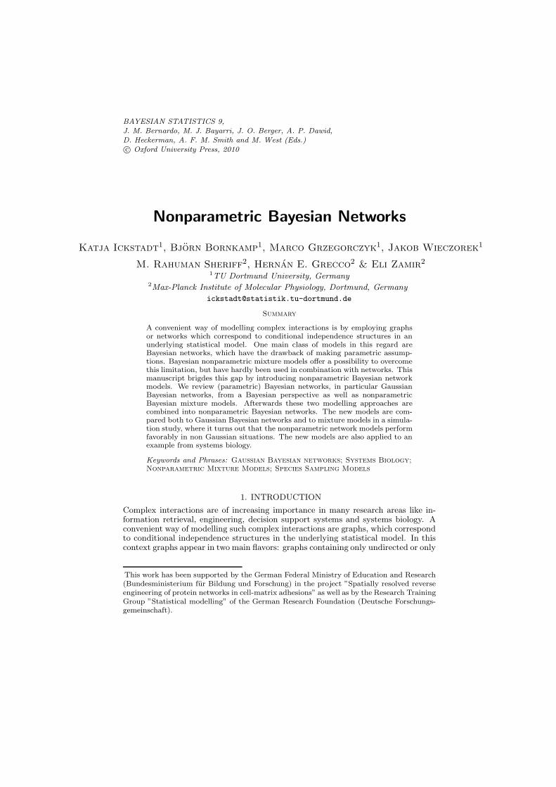
Since sample sizes in experimental data are often limited we consider only sam-ples of 50 and 100 observations. The rest is used for test/validation. Figure 1shows a representative subsample of the data; the nonlinear, hyperbolic pattern ofthe relationships is clearly visible, for example, the relationship of A and B. Datasimulation was done with Mathematica 7.0 (Research, 2008).

For specifying the NPBN model, we applied the general methodology describedin Section 3, by using a random probability measure specified as follows. We useda Poisson distribution with parameter ( = 1 for the number of components N ; con-ditional on N , a symmetric Dirichlet distribution was used for the weights wh withan N dimensional parameter vector (', . . . , '), where we chose ' = 1. The EPPF of

Nonparametric Bayesian Networks 13

A

0.0 1.0 2.0 3.0 1 2 3 4 1.0 2.0 3.0

0.0

1.5

3.0

0.0

1.5

3.0

B

AB

12

34

12

34

C

D

0.5

2.0

3.5

0.0 1.0 2.0 3.0

1.0

2.0

3.0

1 2 3 4 0.5 1.5 2.5 3.5

CD

Figure 1: Scatterplots of the generated data, representative subsample of size100.

14 Ickstadt et al.

such a random probability measure is proportional to N!(N!k(n))!

%k(n)h=1

!(#+nh)!(#) (Lau

and Green, 2007). Note that the EPPF depends on both the unknown parameterN and ', so that essentially two parameters control the flexibility of the clusteringbehavior. While we fixed ' in the simulations, we used a prior distribution for N .For the normal Wishart prior distribution we used the identity matrix for the priorprecision matrix and chose the degrees of freedom parameter equal to d + 2 to en-sure propriety of the prior distribution. The mean vector of the multivariate normaldistribution was chosen as a vector of zeros. The prior distribution on the space ofDAGs was chosen as the prior by Friedman and Koller (2003), which is uniform overthe cardinalities of parent sets. The overall posterior distribution for the allocationvector and the target for MCMC simulations is hence given by

p(l,G, N |X) =#

h

L(G|X(Ih))pN(n)p(N)p(G), (12)

where p(N) is a Poisson distribution with parameter 1.The BGe algorithm was applied using the same normal Wishart prior distri-

bution, while the NPM algorithm was applied using the same specification for therandom probability measure, with the DAG assumed to be fixed and completelyconnected.

To analyze the data we used the MCMC algorithm outlined in Section 3 anddescribed in more detail in the Appendix. We conducted several runs for the NPBNmodel and the reference models BGe and NPM, for both sample sizes 50 and 100.We present in detail a run with 4 · 106 iterations with thinning of 2000 and a burnin of 1 ·106 iterations. We initialized the allocation vector with allocations obtainedfrom the k-means algorithm with 10 components. This has two advantages: (i)The algorithm starts in a region of the posterior distribution with potentially largeposterior mass and (ii) using a larger number of components as initialization isbeneficial as the merge step of the algorithm is more e"ective (see Appendix). Forboth NPBN and NPM the same clusterings were used.

In order to compare the performance of the three di"erent approaches we com-puted the posterior predictive probability (ppp) for the simulated data which hasnot been used to train the system. For one data point xtest the ppp is calculatedby

p(xtest) =

'

p(xtest|#m). /0 1

likelihood

p(#m|xtrain1 , . . . ,xtrain

n )d#m

with m # {BGe, NPM, NPBN}. The overall ppp on log scale for all test data equals

log

2

3

ntest#

i=1

p(xtesti )

4

5 =ntest(

i=1

log p(xtesti )

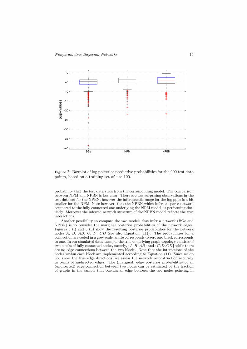
with higher values corresponding to a better model.Figure 2 shows the results of the log ppp for the test data. The training data

consisted of 100 observations. It can be seen that the NPM and NPBN performbetter than the BGe model. This is possibly due to the non-linearity in the rela-tionship between the variables (see also Figure 1). Both the mean of the log ppp inTable 1 and the quantiles visible in Figure 2 are larger for NPBN and NPM. Thisis also indicated by the probabilities in Table 1, which can be interpreted as the

Nonparametric Bayesian Networks 15

BGe NPM NPBN−40

−35

−30

−25

−20

−15

−10

−5

0

ppp−values

Figure 2: Boxplot of log posterior predictive probabilities for the 900 test datapoints, based on a training set of size 100.

probability that the test data stem from the corresponding model. The comparisonbetween NPM and NPBN is less clear: There are less surprising observations in thetest data set for the NPBN, however the interquartile range for the log ppps is a bitsmaller for the NPM. Note however, that the NPBN which infers a sparse networkcompared to the fully connected one underlying the NPM model, is performing sim-ilarly. Moreover the inferred network structure of the NPBN model reflects the trueinteractions.

Another possibility to compare the two models that infer a network (BGe andNPBN) is to consider the marginal posterior probabilities of the network edges.Figures 3 (i) and 3 (ii) show the resulting posterior probabilities for the networknodes A, B, AB, C, D, CD (see also Equation (11)). The probabilities for aconnection are coded in a grey scale, white corresponds to zero and black correspondsto one. In our simulated data example the true underlying graph topology consists oftwo blocks of fully connected nodes, namely, {A,B,AB} and {C,D,CD} while thereare no edge connections between the two blocks. Note that the interactions of thenodes within each block are implemented according to Equation (11). Since we donot know the true edge directions, we assess the network reconstruction accuracyin terms of undirected edges. The (marginal) edge posterior probabilities of an(undirected) edge connection between two nodes can be estimated by the fractionof graphs in the sample that contain an edge between the two nodes pointing in

16 Ickstadt et al.

Sample Size BGe NPM NPBN

50 mean -5.5943 -5.0128 -5.0245model probability 0.22 0.39 0.39

100 mean -5.5512 -4.4677 -4.3971model probability 0.13 0.41 0.46

Table 1: Predictive probabilities for both samples (50 and 100 observations).

either direction. For our 6-node network example the posterior probabilities of allpossible undirected edge connections leads to a symmetric 6 " 6 matrix. Figure 3shows heatmaps for this matrix for BGe (panel (i)) and NPBN (panel (ii)). Itcan be seen that the NPBN model, overall, assigns higher posterior probabilitiesto the edges within the two blocks than the BGe model. For the standard BGemodel the node AB is neither connected with node A nor with node B. Moreover,the posterior probability of the edge connection D , CD is only of moderate size(medium grey).The more sophisticated NPBN model assigns the highest posteriorprobability to four of the six true gold standard edge connections (black elementsin Figure 3). Furthermore, the true edge A, AB at least appears in medium grey.Its posterior probabiliy is comparable to the posterior probability of two falses edgeconnections: C,AB and D,AB. Overall, the heatmaps indicate that NPBN givesa better network reconstruction accuracy than the standard BGe model.

(i)

A B AB C D CD

A

B

AB

C

D

CD

(ii)

A B AB C D CD

A

B

AB

C

D

CD

Figure 3: Heatmap inferred from the data set with 50 observations; represen-tations of the (marginal) posterior probabilities of undirected edges, panel (i)BGe and panel (ii) NPBN. In both panels columns and rows represent thenodes A, B, AB, C, D, and CD, and a grey shading is used to indicate theposterior probabilities (black corresponds to 1, and white corresponds to 0).

Nonparametric Bayesian Networks 17

REFERENCES

Bornkamp, B. and Ickstadt, K. (2009) Bayesian nonparametric estimation ofcontinuous monotone functions with applications to dose-response analysis, Bio-metrics 65, 198–205.

Carvalho, C. M. and Scott, J. G. (2010) Objective Bayesian model selection inGaussian graphical models, Biometrika xx, xx–xx.

Clyde, M. A. and Wolpert, R. L. (2007) Nonparametric function estimationusing overcomplete dictionaries, in J. M. Bernardo, M. J. Bayarri, J. O. Berger,A. P. Dawid, D. Heckerman, A. F. M. Smith and M. West (eds.), Bayesian Statis-tics 8, Oxford University Press, pp. 91–114.

Cooper, G. F. and Herskovits, E. (1992) A Bayesian method for the inductionof probabilistic networks from data, Machine Learning 9, 309–347.

Escobar, M. D. and West, M. (1995) Bayesian density estimation using mixtures,Journal of the American Statistical Association 90, 577–588.

Ferguson, T. S. (1973) A Bayesian analysis of some nonparametric problems,Annals of Statistics 1, 209–230.

Friedman, N. and Koller, D. (2003) Being Bayesian about network structure,Machine Learning 50, 95–126.

Friedman, N., Linial, M., Nachman, I. and Pe’er, D. (2000) Using Bayesiannetworks to analyze expression data, Journal of Computational Biology 7, 601–620.

Fruhwirth-Schnatter, S. (2006) Finite Mixture and Markov Switching Models,Springer, Berlin.

Geiger, D. and Heckerman, D. (1994) Learning Gaussian networks, in R. L. deMantaras and D. Poole (eds.), Uncertainty in Artificial Intelligence Proceedingsof the Tenth Conference, pp. 235–243.

Ghosh, J. K. and Ramamoorthi, R. V. (2003) Bayesian Nonparametrics,Springer, New York.

Giudici, P. (1996) Learning in graphical Gaussian models, in J. M. Bernardo, J. O.Berger, A. P. Dawid and A. F. M. Smith (eds.), Bayesian Statistics 5, OxfordUniversity Press, Oxford, pp. 621–628.

Grzegorczyk, M. and Husmeier, D. (2008) Improving the structure MCMCsampler for Bayesian networks by introducing a new edge reversal move, MachineLearning 71, 265–305.

Grzegorczyk, M., Husmeier, D., Edwards, K., Ghazal, P. and Mil-lar, A. (2008) Modelling non-stationary gene regulatory processes with anon-homogeneous Bayesian network and the allocation sampler, Bioinformatics24(18), 2071–2078.

Ishwaran, H. and James, L. F. (2001) Gibbs sampling methods for stick-breakingpriors, Journal of the American Statistical Association 96, 161–173.

18 Ickstadt et al.

Ishwaran, H. and James, L. F. (2003) Generalized weighted Chinese restaurantprocesses for species sampling mixture models, Statistica Sinica 13, 1211–1235.

James, L. F., Lijoi, A. and Prunster, I. (2009) Posterior analysis for normalizedrandom measures with independent increments, Scandinavian Journal of Statis-tics 36, 76–97.

Jordan, M. I. (1999) Learning in Graphical Models, MIT Press.

Kalli, M., Griffin, J. E. and Walker, S. G. (2010) Slice sampling mixturemodels, Statistics and Computing 00, 00–00.

Kholodenko, B. (2000) Negative feedback and ultrasensitivity can bring aboutoscillations in the mitogen-activated protein kinase cascades, European Journalof Biochemistry 267, 1583–1588.

Koller, D. and Friedmann, N. (2009) Probabilistic Graphical Models - Principlesand Techniques, MIT press.

Koski, T. and Noble, J. M. (2009) Bayesian Networks - An Introduction, Wiley.

Lau, J. W. and Green, P. J. (2007) Bayesian model based clustering procedures,Journal of Computational and Graphical Statistics 16, 526–558.

Lee, J., Quintana, F. A., Muller, P. and Trippa, L. (2008) Defining predictiveprobability functions for species sampling models, Technical report, MD AndersonCancer Center.

Madigan, D. and York, J. (1995) Bayesian graphical models for discrete data,International Statistical Review 63, 215–232.

Mukherjee, S. and Speed, T. P. (2008) Network inference using informativepriors, Proceedings of the National Academy of Sciences 105, 14313–14318.

Neal, R. (2000) Markov chain sampling methods for Dirichlet process mixturemodels, Journal of Computational and Graphical Statistics 9, 249–265.

Nobile, A. and Fearnside, A. T. (2007) Bayesian finite mixtures with an un-known number of components, Statistics and Computing 17, 147–162.

Ongaro, A. and Cattaneo, C. (2004) Discrete random probability measures: Ageneral framework for nonparametric Bayesian inference, Statistics and Probabil-ity Letters 67, 33–45.

Pearl, J. (1985) A model of self-activated memory for evidential reasoning, inProceedings of the 7th Conference of the Cognitive Science Society, University ofCalifornia, Irvine, CA, pp. 329–334.

Pearl, J. (1988) Probabilistic Reasoning in Intelligent Systems: Networks of Plau-sible Inference, Morgan Kaufmann, San Francisco, CA, USA.

Pitman, J. (1996) Some developments of the Blackwell-MacQueen urn scheme, inT. S. Ferguson, L. S. Shapley and J. B. MacQueen (eds.), Statistics, Probabilityand Game Theory: Papers in Honor of David Blackwell, Institute of Mathemat-ical Statistics, pp. 245–268.

Nonparametric Bayesian Networks 19

Pitman, J. (2002) Combinatorial Stochastic Processes, Springer.

Research, W. (2008) Mathematica Edition: Version 7.0.

Rodriguez, A., Lenkoski, A. and Dobra, A. (2010) Sparse covariance estimationin heterogeneous samples.URL: http://arxiv.org/abs/1001.4208

Shachter, R. and Kenley, C. (1989) Gaussian influence diagrams, ManagementScience 35, 527–550.

Verma, P. and Pearl, J. (1992) An algorithm for deciding if a set of observed in-dependencies has a causal explanation, in D. Dubois, M. Welman, B. D’Ambrosioand P. Smets (eds.), Uncertainty in Artificial Intelligence Proceedings of theEighth Conference, pp. 323–330.

Wu, Y. and Ghosal, S. (2008) Kullback Leibler property of kernel mixture priorsin Bayesian density estimation, Electronic Journal of Statistics 2, 298–331.

APPENDIX

Appendix: MCMC-Sampler

Here we describe the MCMC sampler used for analysing the NPBN model pro-posed in this paper. The BGe and the NPM model are analysed with the samealgorithm, by only updating the graph (with all observations allocated to one com-ponent) or only updating the allocations (with a completely connected DAG). TheAppendix is based on Grzegorczyk et al. (2008) and Nobile and Fearnside (2007),where a more detailed description can be found.

The MCMC sampler generates a sample from the joint posterior distributionof l,G, N given in Equation (12) and comprises six di"erent types of moves inthe state-space [l,G, N ]. Before the MCMC simulation is started, probabilitiespi (i = 1, . . . , 6) with p1 + · · · + p6 = 1 must be predefined with which one ofthese move types is selected. The moves consist of a structure move, that proposesa change in the graph (abbreviated by DAG move) and five moves that change theallocations (abbreviated by Gibbs, M1, M2 , split and merge). Below we will de-scribe these di"erent move types in some detail.

DAG moveThe first move type is a classical structure MCMC single edge operation on the graphG while the number of components N and the allocation vector l are left unchanged(Madigan and York, 1995). According to the transition probability distribution

q(G|G) =

61

|N (G)| , G # N (G)

0 , G /# N (G)(13)

a new graph G is proposed, and the new state [G, N, l] is accepted according to

A(G|G) =p(G|X)p(G|X)

·q(G|G)

q(G|G)

20 Ickstadt et al.

where |N (G)| is the number of neighbors of the DAG G, that can be reached fromthe current graph by one single edge operation and p(G|X) is defined in (2) for theBGe model and by (12) for the NPBN model.

Allocation movesThe five other move types are adapted from Nobile and Fearnside (2007) and oper-ate on l or on N and l. If there are N > 2 mixture components, then moves of thetype M1 and M2 can be used to re-allocate some observations from one componenth to another one h. That is, a new allocation vector l is proposed while G andN are left unchanged. The split and merge moves change N and l. A split moveproposes to increase the number of mixture components by 1 and simultaneouslytries to re-allocate some observations to fill the new component. The merge move iscomplementary to the split move and decreases the number of mixture componentsby 1. The acceptance probabilities for M1, M2, split and merge are of the samefunctional form

A(l|l) =

7

1,p(l,G, N |X)p(l,G, N |X)

q(l|l)

q(l|l),

8

, (14)

where the proposal probabilities q(.|.) depend on the move type (M1, M2, split,merge). Finally, the Gibbs move re-allocates only one single observation by sam-pling its new allocation from the corresponding full conditional distribution (seeNobile and Fearnside (2007)) while leaving N and l unchanged. In the following wegive an idea how the allocation moves work, for a detailed description including thecorresponding Metropolis-Hastings acceptance probabilities, see Nobile and Fearn-side (2007).

Gibbs move on the allocation vector lIf there is one component only, symbolically N = 1, select another move type.Otherwise randomly select an observation i among the n available and determineto which component h (1 2 h 2 N) this observation currently belongs. For eachmixture component h = 1, . . . , N replace the i-th entry of the allocation vector l bycomponent h to obtain l(i 3, h). We note that l(i 3, h) is equal to the currentallocation vector l. Subsequently, sample the i,th entry of the new allocation vectorl from the corresponding multinomial full conditional distribution.

The M1 move on the allocation vector lIf there is one component only, symbolically N = 1, select a di"erent type of move.Otherwise randomly select two mixture components h and h among the N avail-able. Draw a random number p from a Beta distribution with parameters equal tothe corresponding hyperparameters of the Dirichlet prior on the mixture weights.Re-allocating each observation currently belonging to the h-th or h-th componentto component h with probability p or to component h with probability 1, p givesthe proposed allocation vector l.

The M2 move on the allocation vector lIf there is one component only, symbolically N = 1, select a di"erent move type.Otherwise randomly select two mixture components h and h among the N availableand then randomly select a group of observations allocated to component h and at-tempt to re-allocate them to component h. If the h-th component is empty the move

Nonparametric Bayesian Networks 21

fails outright. Otherwise draw a random number u from a uniform distribution on1, . . . , nh where nh is the number of observations allocated to the h-th component.Subsequently, randomly select u observations from the nh in component h and al-locate the selected observations to component h to obtain the proposed allocationvector l.

The split moveRandomly select a mixture component h (1 2 h < N) as the ejecting component.Draw pE from a Beta(a, a) distribution with a > 0 and re-allocate each observationcurrently allocated to component h in the vector l with probability pE to a newcomponent with label N + 1. Subsequently swap the labels of the new mixturecomponent N +1 with a randomly chosen mixture component label h including thelabel N +1 of the ejected component itself (1 2 h 2 N +1) to obtain the proposedallocation vector l.

The merge moveRandomly select a mixture component h (1 2 h 2 N) as the absorbing componentand another component h (1 2 h 2 N) with h '= h as the disappearing component.Re-allocate all observations currently allocated to the disappearing component h byl to component h to obtain the new allocation vector l. Then delete the (empty)component h to obtain the new number of components N = N , 1.

A disadvantage of the split move is the fact that allocations are chosen randomlyto form the new mixture component. A way to partially overcome this problem isto use informative starting values of the algorithm. One approach with which wehave made good experience is to start the sampler based on the result of a k-meansclustering with a large number of components. The merge move then rather quicklyfinds a good allocation of the mixture components.