Embed Size (px)
Citation preview

arX
iv:1
611.
0931
1v2
[nu
cl-t
h] 1
1 Fe
b 20
17
Nonlocal energy density functionals for pairing and
beyond-mean-field calculations
K. Bennaceur1,2,3, A. Idini2,4, J. Dobaczewski2,3,5,6,
P. Dobaczewski7, M. Kortelainen2,3, and F. Raimondi2,4
1Univ Lyon, Universite Lyon 1, CNRS/IN2P3, IPNL, F-69622 Villeurbanne, France2Department of Physics, PO Box 35 (YFL), FI-40014 University of Jyvaskyla,
Finland3Helsinki Institute of Physics, P.O. Box 64, FI-00014 University of Helsinki, Finland4Department of Physics, University of Surrey, Guildford GU2 7XH, United Kingdom5Department of Physics, University of York, Heslington, York YO10 5DD, United
Kingdom6Institute of Theoretical Physics, Faculty of Physics, University of Warsaw, ul.
Pasteura 5, PL-02-093 Warsaw, Poland7ul. Obozowa 85 m. 5, PL-01425 Warsaw, Poland
Abstract. We propose to use two-body regularized finite-range pseudopotential to
generate nuclear energy density functional (EDF) in both particle-hole and particle-
particle channels, which makes it free from self-interaction and self-pairing, and
also free from singularities when used beyond mean field. We derive a sequence of
pseudopotentials regularized up to next-to-leading order (NLO) and next-to-next-to-
leading order (N2LO), which fairly well describe infinite-nuclear-matter properties and
finite open-shell paired and/or deformed nuclei. Since pure two-body pseudopotentials
cannot generate sufficiently large effective mass, the obtained solutions constitute a
preliminary step towards future implementations, which will include, e.g., EDF terms
generated by three-body pseudopotentials.

Nonlocal energy density functionals for pairing and beyond-mean-field calculations 2
1. Introduction
The two most widely used families of non-relativistic nuclear energy density functionals
(EDFs) are based on the Skyrme [1, 2] and Gogny [3] functional generators. The main
difference between them is that the Skyrme-type generators are built as sums of contact
terms with nonlocal gradient corrections, whereas the Gogny-type ones are built as
sums of local finite-range Gaussians. In Gogny and most Skyrme parametrizations, to
conveniently reproduce properties of homogeneous nuclear matter, a two-body density-
dependent generator is usually used, most often with a fractional power of the density.
Unfortunately, such an approach leads to non-analytic properties of beyond-mean-field
EDF in the complex plane [4], compromises symmetry-restoration procedures [5, 4, 6],
and introduces self-interaction contributions in the particle-vibration coupling vertex [7].
Thus, to gain progress in the development of a consistent description of atomic
nucleus, there clearly appears a need to build EDFs that are free from the above
spuriousities. Such functionals can be obtained by defining their potential parts
as Hartree-Fock-Bogolyubov (HFB) expectation values of genuine pseudopotential
operators. In fact, this was the original idea of Skyrme who first introduced the name
pseudopotential in this context [8]. Without density-dependent terms and taking all
exchange and pairing terms into account, this gives EDFs for which the Pauli principle
is strictly obeyed and removes all spurious contributions. Following Refs. [9, 10], also
here we call such pseudopotentials EDF generators.
In Refs. [11, 12, 13, 9], we have already fully developed the formalism that uses
contact and regularized higher-order pseudopotentials to generate the most general
terms in the EDF compatible with symmetries. There were several recent attempts
to use such EDFs, like the development of the Skyrme–inspired family of functionals
SLyMR which include 3- and 4-body terms [14], our previous parametrization of
the regularized finite-range pseudopotential REG2 [15], or functional VLyB, which
implemented higher-order contact terms [16]. However none of the previous attempts
managed to reproduce both bulk and pairing properties of finite nuclei, while ensuring
at the same time stability of homogeneous nuclear matter.
The aim of this article is thus to present a further step in the construction
of a predictive pseudopotential-based EDF. We present an adjustment of a
parametrization of the regularized finite-range higher-order local and density-
independent pseudopotential, which achieves an acceptable qualitative description both
in the particle-hole and particle-particle channels without leading to infinite-matter
instabilities. With the limitation of the current implementation being only purely two-
body and local, a sufficiently high value of the infinite-matter effective mass could not
be obtained. However, reasonably good results obtained for bulk and pairing properties
of finite nuclei demonstrate proof-of-principle feasibility of such program.
The article is organized as follows. In section 2 we briefly recall the form of the
pseudopotential and present the corresponding EDF terms in particle-hole and particle-
particle channels. The numerical implementation of the mean-field equations in the
Nonlocal energy density functionals for pairing and beyond-mean-field calculations 3
new HFB spherical solver finres4 is briefly discussed in section 3. The strategy used to
adjust the parameters is given in section 4. In section 5 we discuss statistical errors of
the resulting parameters and observables, and present selected results for infinite nuclear
matter and finite nuclei. Conclusions are given in section 6.
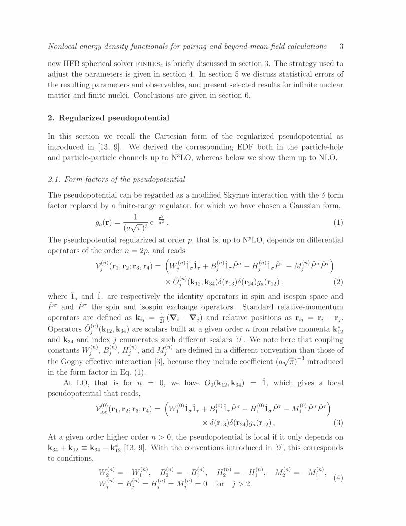
2. Regularized pseudopotential
In this section we recall the Cartesian form of the regularized pseudopotential as
introduced in [13, 9]. We derived the corresponding EDF both in the particle-hole
and particle-particle channels up to N3LO, whereas below we show them up to NLO.
2.1. Form factors of the pseudopotential
The pseudopotential can be regarded as a modified Skyrme interaction with the δ form
factor replaced by a finite-range regulator, for which we have chosen a Gaussian form,
ga(r) =1
(a√π)3
e−r2
a2 . (1)
The pseudopotential regularized at order p, that is, up to NpLO, depends on differential
operators of the order n = 2p, and reads
V(n)j (r1, r2; r3, r4) =
(
W(n)j 1σ1τ +B
(n)j 1τ P
σ −H(n)j 1σP
τ −M(n)j P σP τ
)
× O(n)j (k12,k34)δ(r13)δ(r24)ga(r12) . (2)
where 1σ and 1τ are respectively the identity operators in spin and isospin space and
P σ and P τ the spin and isospin exchange operators. Standard relative-momentum
operators are defined as kij = 12i(∇i −∇j) and relative positions as rij = ri − rj.
Operators O(n)j (k12,k34) are scalars built at a given order n from relative momenta k∗
12
and k34 and index j enumerates such different scalars [9]. We note here that coupling
constants W(n)j , B
(n)j , H
(n)j , and M
(n)j are defined in a different convention than those of
the Gogny effective interaction [3], because they include coefficient (a√π)
−3introduced
in the form factor in Eq. (1).
At LO, that is for n = 0, we have O0(k12,k34) = 1, which gives a local
pseudopotential that reads,
V(0)loc (r1, r2; r3, r4) =
(
W(0)1 1σ1τ +B
(0)1 1τ P
σ −H(0)1 1σP
τ −M(0)1 P σP τ
)
× δ(r13)δ(r24)ga(r12) , (3)
At a given order higher order n > 0, the pseudopotential is local if it only depends on
k34 + k12 ≡ k34 − k∗12 [13, 9]. With the conventions introduced in [9], this corresponds
to conditions,
W(n)2 = −W
(n)1 , B
(n)2 = −B
(n)1 , H
(n)2 = −H
(n)1 , M
(n)2 = −M
(n)1 ,
W(n)j = B
(n)j = H
(n)j = M
(n)j = 0 for j > 2.
(4)
Nonlocal energy density functionals for pairing and beyond-mean-field calculations 4
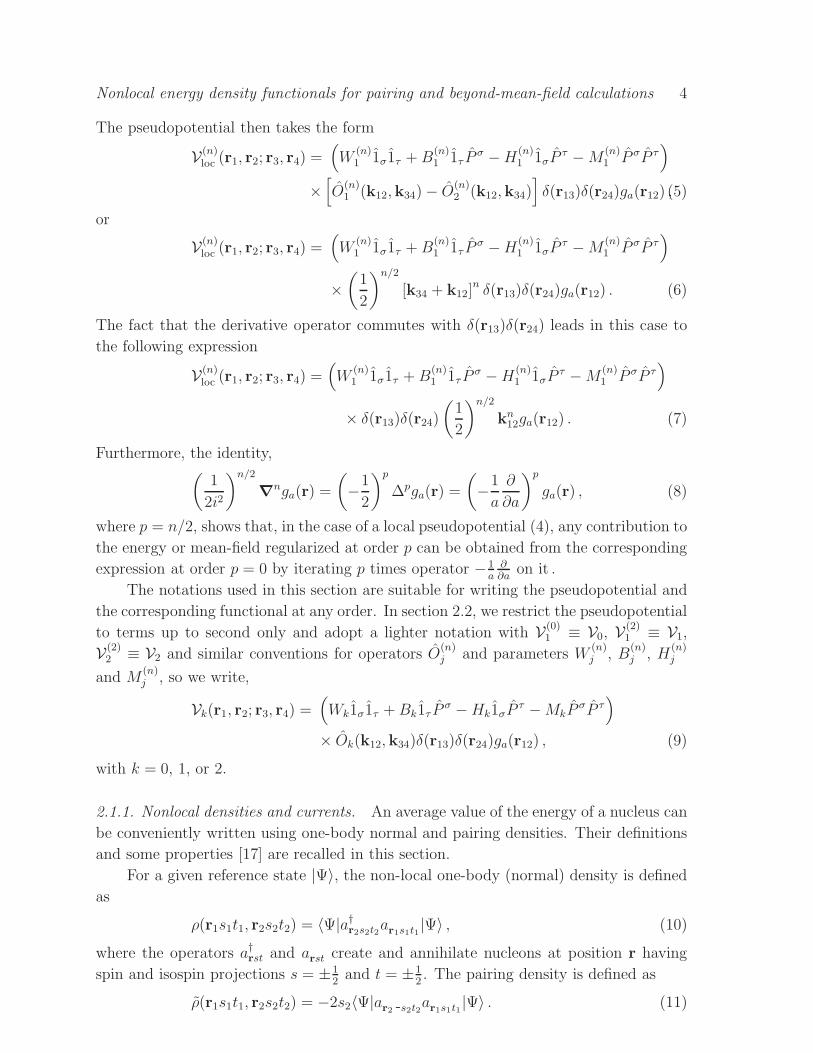
The pseudopotential then takes the form
V(n)loc (r1, r2; r3, r4) =
(
W(n)1 1σ1τ +B
(n)1 1τ P
σ −H(n)1 1σP
τ −M(n)1 P σP τ
)
×[
O(n)1 (k12,k34)− O
(n)2 (k12,k34)
]
δ(r13)δ(r24)ga(r12) ,(5)
or
V(n)loc (r1, r2; r3, r4) =
(
W(n)1 1σ1τ +B
(n)1 1τ P
σ −H(n)1 1σP
τ −M(n)1 P σP τ
)
×(
1
2
)n/2
[k34 + k12]n δ(r13)δ(r24)ga(r12) . (6)
The fact that the derivative operator commutes with δ(r13)δ(r24) leads in this case to
the following expression
V(n)loc (r1, r2; r3, r4) =
(
W(n)1 1σ1τ +B
(n)1 1τ P
σ −H(n)1 1σP
τ −M(n)1 P σP τ
)
× δ(r13)δ(r24)
(
1
2
)n/2
kn12ga(r12) . (7)
Furthermore, the identity,(
1
2i2
)n/2
∇nga(r) =
(
−1
2
)p
∆pga(r) =
(
−1
a
∂
∂a
)p
ga(r) , (8)
where p = n/2, shows that, in the case of a local pseudopotential (4), any contribution to
the energy or mean-field regularized at order p can be obtained from the corresponding
expression at order p = 0 by iterating p times operator − 1a
∂∂a
on it .
The notations used in this section are suitable for writing the pseudopotential and
the corresponding functional at any order. In section 2.2, we restrict the pseudopotential
to terms up to second only and adopt a lighter notation with V(0)1 ≡ V0, V(2)
1 ≡ V1,
V(2)2 ≡ V2 and similar conventions for operators O
(n)j and parameters W
(n)j , B
(n)j , H
(n)j
and M(n)j , so we write,
Vk(r1, r2; r3, r4) =(
Wk1σ1τ +Bk1τ Pσ −Hk1σP
τ −MkPσP τ
)
× Ok(k12,k34)δ(r13)δ(r24)ga(r12) , (9)
with k = 0, 1, or 2.
2.1.1. Nonlocal densities and currents. An average value of the energy of a nucleus can
be conveniently written using one-body normal and pairing densities. Their definitions
and some properties [17] are recalled in this section.
For a given reference state |Ψ〉, the non-local one-body (normal) density is defined
as
ρ(r1s1t1, r2s2t2) = 〈Ψ|a†r2s2t2ar1s1t1 |Ψ〉 , (10)
where the operators a†rst and a
rst create and annihilate nucleons at position r having
spin and isospin projections s = ±12and t = ±1
2. The pairing density is defined as
ρ(r1s1t1, r2s2t2) = −2s2〈Ψ|ar2 -s2t2ar1s1t1 |Ψ〉 . (11)

Nonlocal energy density functionals for pairing and beyond-mean-field calculations 5
These two densities satisfy the properties
ρ(r1s1t1, r2s2t2) = ρ∗(r2s2t2, r1s1t1) , (12)
ρ(r1s1t1, r2s2t2) = 4s1s2 ρ(r2 -s2t2, r1 -s1t1) . (13)
In the present article, we do not consider the possibility to mix protons and
neutrons. This restriction has the consequence that the normal and pairing densities
are diagonal in the neutron-proton space. In this situation, the normal density can be
expanded in (iso)scalar/(iso)vector parts using identity and Pauli matrices as
ρ(r1s1t1, r2s2t2) =14ρ0(r1, r2)δs1s2δt1t2 +
14ρ1(r1, r2)δs1s2τ
(3)t1t2
+ 14s0(r1, r2) · σs1s2δt1t2 +
14s1(r1, r2) · σs1s2τ
(3)t1t2 , (14)
and the pairing density as
ρ(r1s1t, r2s2t) =12ρt(r1, r2)δs1s2 +
12st(r1, r2) · σs1s2 . (15)
In the latter expression, index t = n or p stands for neutrons or protons, respectively.
Since the pseudopotential may contain derivative terms, we introduce the following
nonlocal densities
τT (r1, r2) = ∇1 ·∇2 ρT (r1, r2) , (16)
TT (r1, r2) = ∇1 ·∇2 sT (r1, r2) , (17)
jT (r1, r2) =12i(∇1 −∇2) ρT (r1, r2) , (18)
JTµν(r1, r2) =12i(∇1 −∇2)µ sTν(r1, r2) (19)
which are respectively the nonlocal scalar kinetic, pseudo-vector spin-kinetic, vector
current and spin-orbit tensor densities. In these expressions, index T = 0 or 1 stands
for isoscalar or isovector densities, respectively and µ and ν represent the Cartesian
coordinates in directions x, y and z. In a similar manner, we introduce the following
non-local pairing densities
τt(r1, r2) = ∇1 ·∇2 ρt(r1, r2) , (20)
Tt(r1, r2) = ∇1 ·∇2 st(r1, r2) , (21)
t(r1, r2) =12i(∇1 −∇2) ρt(r1, r2) , (22)
Jtµν(r1, r2) =12i(∇1 −∇2)µ stν(r1, r2) . (23)
2.2. Structure of the nonlocal energy density functional
By summing over spin and isospin indices, one obtains contributions to the energy that
come from different terms of the regularized pseudopotential, as given in equation (9).
For given values of k, this energy contains the local part,
〈V Lk 〉 =
∑
T=0,1
∫
d3r1 d3r2 d
3r3 d3r4
[
Ok(k12,k34)δ(r13)δ(r24)ga(r12)]
×[
AρTk ρT (r3, r1)ρT (r4, r2) + AsT
k sT (r3, r1) · sT (r4, r2)]
, (24)
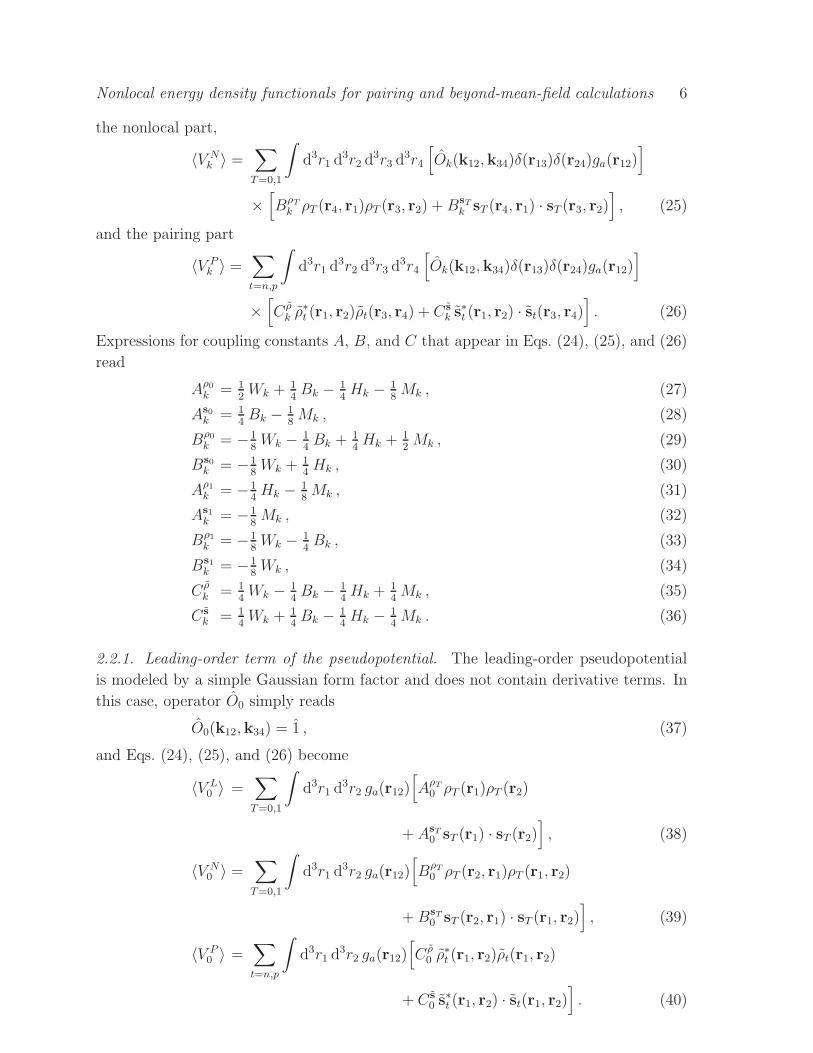
Nonlocal energy density functionals for pairing and beyond-mean-field calculations 6
the nonlocal part,
〈V Nk 〉 =
∑
T=0,1
∫
d3r1 d3r2 d
3r3 d3r4
[
Ok(k12,k34)δ(r13)δ(r24)ga(r12)]
×[
BρTk ρT (r4, r1)ρT (r3, r2) +BsT
k sT (r4, r1) · sT (r3, r2)]
, (25)
and the pairing part
〈V Pk 〉 =
∑
t=n,p
∫
d3r1 d3r2 d
3r3 d3r4
[
Ok(k12,k34)δ(r13)δ(r24)ga(r12)]
×[
C ρk ρ
∗t (r1, r2)ρt(r3, r4) + C s
k s∗t (r1, r2) · st(r3, r4)
]
. (26)
Expressions for coupling constants A, B, and C that appear in Eqs. (24), (25), and (26)
read
Aρ0k = 1
2Wk +
14Bk − 1
4Hk − 1
8Mk , (27)
As0
k = 14Bk − 1
8Mk , (28)
Bρ0k = −1
8Wk − 1
4Bk +
14Hk +
12Mk , (29)
Bs0
k = −18Wk +
14Hk , (30)
Aρ1k = −1
4Hk − 1
8Mk , (31)
As1
k = −18Mk , (32)
Bρ1k = −1
8Wk − 1
4Bk , (33)
Bs1
k = −18Wk , (34)
C ρk = 1
4Wk − 1
4Bk − 1
4Hk +
14Mk , (35)
C s
k = 14Wk +
14Bk − 1
4Hk − 1
4Mk . (36)
2.2.1. Leading-order term of the pseudopotential. The leading-order pseudopotential
is modeled by a simple Gaussian form factor and does not contain derivative terms. In
this case, operator O0 simply reads
O0(k12,k34) = 1 , (37)
and Eqs. (24), (25), and (26) become
〈V L0 〉 =
∑
T=0,1
∫
d3r1 d3r2 ga(r12)
[
AρT0 ρT (r1)ρT (r2)
+ AsT
0 sT (r1) · sT (r2)]
, (38)
〈V N0 〉 =
∑
T=0,1
∫
d3r1 d3r2 ga(r12)
[
BρT0 ρT (r2, r1)ρT (r1, r2)
+BsT
0 sT (r2, r1) · sT (r1, r2)]
, (39)
〈V P0 〉 =
∑
t=n,p
∫
d3r1 d3r2 ga(r12)
[
C ρ0 ρ
∗t (r1, r2)ρt(r1, r2)
+ C s
0 s∗t (r1, r2) · st(r1, r2)
]
. (40)

Nonlocal energy density functionals for pairing and beyond-mean-field calculations 7
2.2.2. Next-to-leading order term of the pseudopotential At NLO, the two derivative
operators are
O1(k12,k34) =12
(
k∗212 + k2
34
)
, (41)
and
O2(k12,k34) = k∗12 · k34 , (42)
The contribution from the first one to the EDF is given by
〈V L1 〉 = 1
2
∑
T=0,1
∫
d3r1 d3r2 ga(r12)
×{
AρT1
[
τT (r1)ρT (r2)− 34ρT (r1)∆2ρT (r2)− jT (r1) · jT (r2)
]
+ AsT
1
[
TT (r1) · sT (r2)− 34sT (r2) ·∆1sT (r1)
−∑
µν
JTµν(r1)JTµν(r2)]}
, (43)
〈V N1 〉 = − 1
2
∑
T=0,1
∫
d3r1 d3r2
×{1
2∆ga(r12) [B
ρT1 ρT (r2, r1)ρT (r1, r2) +BsT
1 sT (r2, r1) · sT (r1, r2)]
+ BρT1 ga(r12)
[
ρT (r2, r1)τT (r1, r2) + ρT (r2, r1)∆1ρT (r1, r2)]
+ BsT
1 ga(r12)[
sT (r2, r1) ·TT (r1, r2) + sT (r2, r1) ·∆1sT (r1, r2)]}
,(44)
and
〈V P1 〉 = 1
2
∑
t=n,p
∫
d3r1 d3r2 ga(r12)
×{
C ρ1
[
ρ∗t (r1, r2)τt(r1, r2)− ρ∗t (r1, r2)∆1ρt(r1, r2)]
+ C s
1
[
s∗t (r1, r2) · Tt(r1, r2)− s∗t (r1, r2) ·∆1st(r1, r2)]}
, (45)
and in turn the contribution from the second one is
〈V L2 〉 = 1
2
∑
T=0,1
∫
d3r1 d3r2 ga(r12)
×{
AρT2
[
ρT (r1)τT (r2) +14ρT (r1)∆2ρT (r2)− jT (r1) · jT (r2)
]
+ AsT
2
[
sT (r1) ·TT (r2) +14sT (r2) ·∆1sT (r1)
−∑
µν
JTµν(r1)JTµν(r2)]}
, (46)
〈V N2 〉 = 1
2
∑
T=0,1
∫
d3r1 d3r2

Nonlocal energy density functionals for pairing and beyond-mean-field calculations 8
×{1
2∆ga(r12) [B
ρT2 ρT (r2, r1)ρT (r1, r2) +BsT
2 sT (r2, r1) · sT (r1, r2)]
− BρT2 ga(r12)
[
ρT (r2, r1)∆1ρT (r1, r2) + ρT (r2, r1)τT (r1, r2)]
− BsT
2 ga(r12)[
sT (r2, r1) ·∆1sT (r1, r2) + sT (r2, r1) ·TT (r1, r2)]}
,(47)
and
〈V P2 〉 = 1
2
∑
t=n,p
∫
d3r1 d3r2
×{
∆ga(r12)[
C ρ2 ρ
∗t (r1, r2)ρt(r1, r2) + C s
2 s∗t (r1, r2) · st(r1, r2)
]
+ C ρ2ga(r12)
[
ρ∗t (r1, r2)τt(r1, r2)− ρ∗t (r1, r2)∆1ρt(r1, r2)]
+ C s
2ga(r12)[
s∗t (r1, r2) · Tt(r1, r2)− s∗t (r1, r2) ·∆1st(r1, r2)]}
. (48)
2.2.3. Sum of pseudopotential terms at NLO. The sum of the terms at NLO leads to the
expression where contributions from the local and nonlocal parts of the pseudopotential
can be explicitly separated. This leads to a form where we can take advantage of
property (8), and which is therefore simpler to implement numerically.
Before we write down the sum of terms given by the two NLO pseudopotential
terms, it is convenient to introduce the following notation for half sum and half difference
of the NLO coupling constants, for example
Aρ012 =
1
2(Aρ0
1 + Aρ02 ) , (49)
Aρ012
=1
2(Aρ0
1 − Aρ02 ) . (50)
This notation allows us to separate terms of the functional that come from the local
part of the pseudopotential (parameterized by terms with indices 12) from those that
come from the nonlocal part of pseudopotential (parameterized by terms with indices
12). The sum of NLO terms shown in section 2.2.2 then reads
〈V L1 〉+ 〈V L
2 〉 =∑
T=0,1
∫
d3r1 d3r2
×{
AρT12 ga(r12)
[
τT (r1)ρT (r2)− 14ρT (r1)∆2ρT (r2)− jT (r1) · jT (r2)
]
+ AsT
12 ga(r12)[
TT (r1) · sT (r2)− 14sT (r2) ·∆1sT (r1)− JT (r1) · JT (r2)
]
− 1
2∆ga(r12)
[
AρT12ρT (r1)ρT (r2) + AsT
12sT (r1) · sT (r2)
]
}
, (51)
〈V N1 〉+ 〈V N
2 〉 = −∑
T=0,1
∫
d3r1 d3r2
×{
BρT12 ga(r12)
[
ρT (r2, r1)∆1ρT (r1, r2) + ρT (r2, r1)τT (r1, r2)]
+ BsT
12 ga(r12)[
sT (r2, r1) ·∆1sT (r1, r2) + sT (r2, r1) ·TT (r1, r2)]
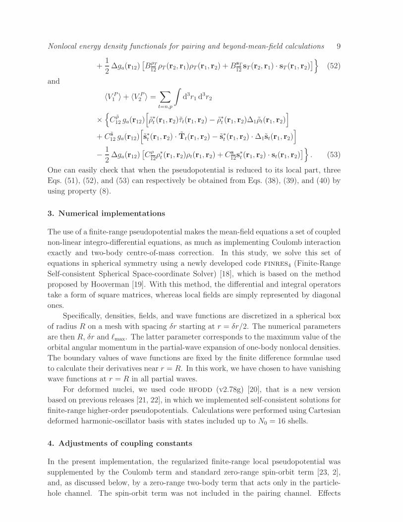
Nonlocal energy density functionals for pairing and beyond-mean-field calculations 9
+1
2∆ga(r12)
[
BρT12ρT (r2, r1)ρT (r1, r2) +BsT
12sT (r2, r1) · sT (r1, r2)
]
}
(52)
and
〈V P1 〉+ 〈V P
2 〉 =∑
t=n,p
∫
d3r1 d3r2
×{
C ρ12 ga(r12)
[
ρ∗t (r1, r2)τt(r1, r2)− ρ∗t (r1, r2)∆1ρt(r1, r2)]
+ C s
12 ga(r12)[
s∗t (r1, r2) · Tt(r1, r2)− s∗t (r1, r2) ·∆1st(r1, r2)]
− 1
2∆ga(r12)
[
Cρ
12ρ∗t (r1, r2)ρt(r1, r2) + Cs
12s∗t (r1, r2) · st(r1, r2)
]
}
. (53)
One can easily check that when the pseudopotential is reduced to its local part, three
Eqs. (51), (52), and (53) can respectively be obtained from Eqs. (38), (39), and (40) by
using property (8).
3. Numerical implementations
The use of a finite-range pseudopotential makes the mean-field equations a set of coupled
non-linear integro-differential equations, as much as implementing Coulomb interaction
exactly and two-body centre-of-mass correction. In this study, we solve this set of
equations in spherical symmetry using a newly developed code finres4 (Finite-Range
Self-consistent Spherical Space-coordinate Solver) [18], which is based on the method
proposed by Hooverman [19]. With this method, the differential and integral operators
take a form of square matrices, whereas local fields are simply represented by diagonal
ones.
Specifically, densities, fields, and wave functions are discretized in a spherical box
of radius R on a mesh with spacing δr starting at r = δr/2. The numerical parameters
are then R, δr and ℓmax. The latter parameter corresponds to the maximum value of the
orbital angular momentum in the partial-wave expansion of one-body nonlocal densities.
The boundary values of wave functions are fixed by the finite difference formulae used
to calculate their derivatives near r = R. In this work, we have chosen to have vanishing
wave functions at r = R in all partial waves.
For deformed nuclei, we used code hfodd (v2.78g) [20], that is a new version
based on previous releases [21, 22], in which we implemented self-consistent solutions for
finite-range higher-order pseudopotentials. Calculations were performed using Cartesian
deformed harmonic-oscillator basis with states included up to N0 = 16 shells.
4. Adjustments of coupling constants
In the present implementation, the regularized finite-range local pseudopotential was
supplemented by the Coulomb term and standard zero-range spin-orbit term [23, 2],
and, as discussed below, by a zero-range two-body term that acts only in the particle-
hole channel. The spin-orbit term was not included in the pairing channel. Effects
Nonlocal energy density functionals for pairing and beyond-mean-field calculations 10
of the spurious centre-of-mass motion were approximately removed by the standard
technique consisting in subtracting from the functional (before variation and without
the one-body approximation) the average value of the momentum squared divided by
twice total mass [24]. Adjustments of coupling constants were performed in spherical
symmetry. For simplicity, small contributions to pairing terms that come from the
spin-orbit interaction were neglected. In addition, for deformed nuclei calculations were
performed with contributions to pairing terms that come from the Coulomb term also
neglected. These two latter restrictions will be released in future implementations.
Coupling constants of the regularized pseudopotential were determined by building
and minimizing a penalty function whose content is discussed below. For a given value
of the regularization range a, the regularized finite-range local pseudopotential (4),
depends on 8 independent parameters at NLO and on 12 at N2LO. The strength of the
spin-orbit interaction makes one additional parameter WSO.
After performing several preliminary adjustments, we noted that pairing fields were
strongly peaked at the nuclear surface. This feature has two unwanted consequences.
Firstly, pairing energies and average gaps were becoming unreasonably strong in neutron
rich isotopes, where a neutron skin develops. Secondly, proton pairing gaps were much
too weak compared to typical expected values. This was due to the fact that the
Coulomb barrier shifts the proton density from the surface to the nuclear interior.
As a solution to these problems, we considered adding to the functional a term
that makes pairing stronger in the volume without increasing its strength at the surface.
Equivalently, the one which balances the finite-range pseudopotential, so that it can be
stronger in the pairing channel, without letting the particle-hole channel becoming too
attractive. This can be achieved by adding a zero-range term of the standard Skyrme
type,
Vδ(r1, r2; r3, r4) = t0
(
1 + x0Pσ)
δ(r13)δ(r24)δ(r12) , (54)
with x0 = 1. This zero-range term indeed allows us to de-correlate the behaviour of
the LO terms in the particle-hole and T = 1 particle-particle channels. Since this term
does not act in the pairing channel, no pairing cut-off is needed. However, when used in
beyond-mean-field applications, this term may still lead to ultra-violet divergence. In
principle, it would be very easy to avoid this by regularizing this term with a short-range
regulator. This route may be exploited in future developments.
A series of tests performed at NLO showed that for regularization ranges between
a = 1.1 and 1.3 fm, the value of t0 = 1000 MeV fm3 leads to a pairing field which is not
too strongly peaked at the surface. In order to limit the number of free parameters, this
value for t0 was fixed and kept constant for all pseudopotentials at NLO and N2LO. We
note that by adopting a fixed value of parameter t0, we removed its influence on the
error budget discussed in section 5.2.

Nonlocal energy density functionals for pairing and beyond-mean-field calculations 11
4.1. The penalty function
The penalty function [25] depends on the vector of parameters of the model p,
χ2(p) =
Nd∑
i=1
(
Oi(p)−Otargeti
)2
∆O2i
, (55)
and measures quadratic deviation between calculated Oi(p) and target Otargeti values
for a set of observables or pseudo-observables with given adopted uncertainties ∆Oi. In
our implementation, we built the penalty function as a sum of six different components,
χ2 = χ2inm + χ2
pol + χ2BE + χ2
rad + χ2gap + χ2
ρ1, (56)
which are defined as follows:
• We constrained the following properties of the saturation point of the infinite
nuclear matter, see [15] for definitions, with their adopted uncertainties: saturation
density ρsat = 0.160 ± 0.0005 fm−3, binding energy per nucleon E/A = −16.00 ±0.05MeV, incompressibility modulus K∞ = 230 ± 1MeV, symmetry energy J =
32.0±0.1MeV and its slope L = 50±10MeV. The sum of contributions from these
properties to the penalty function is denoted χ2inm.
• One value for the energy per nucleon in polarized matter B↑(0.16) = 35 ± 1MeV.
This value does not correspond to the result from a microscopic calculation and
is only considered to prevent the collapse of polarized matter near the saturation
point. We denote the contribution from this constraint to the penalty function as
χ2pol.
• Binding energies and proton radii of several doubly magic and semi-magic nuclei as
summarized in Table 1. Contributions to the penalty function from theses quantities
are denoted χ2BE and χ2
rad, respectively.
• The zero-range term (54) turned out to be useful but not sufficient to guarantee that
the pairing field would not be too strong at the nuclear surface. For that purpose,
we used an additional scheme when constraining average pairing gaps. Since all
our densities are expended in partial waves up to a given value ℓmax, a pairing field
strong at the surface is expected to give a significant change of the results if the
maximum value of ℓ is changed from ℓmax = ℓ0 to ℓmax = ℓ0 + 2. Reciprocally,
an average neutron pairing gap in a given nucleus, which is constrained to give
approximately the same value for calculations with ℓmax = ℓ0 and ℓmax = ℓ0+2 can
prevent the pairing field from being too strong near the surface.
In practice, we constrained the average neutron pairing gap 〈∆n〉 in 120Sn calculated
at ℓmax = 9 and ℓmax = 11. Pseudopotentials considered here lead to a low effective
mass and thus a low density of states. In order to avoid too frequent collapses of
pairing correlations in nuclei with subshells closure or with the opening of gaps for
deformed nuclei, we decided to largely overshoot the value of the average pairing
gap compared to what can be extracted from experimental mass staggering, and
we used the target value of 〈∆n〉 = 2.8MeV for the two values of ℓmax with a small
Nonlocal energy density functionals for pairing and beyond-mean-field calculations 12
uncertainty of 0.002MeV. This ensures that the average pairing gap is almost the
same for the two truncations and therefore the pairing field does not significantly
change when more partial waves are added. The contribution from these constraints
to the penalty function is denoted χ2gap.
• We have observed that the fit of the parameters can easily drive the pseudopotential
into regions of the parameter space that lead to finite-size instabilities similar
to those already identified for Skyrme functionals [26]. For this latter type of
functionals, a tool based on the linear response theory was developed to characterize
and avoid these finite-size instabilities. Such a tool does not yet exist for the
pseudopotentials considered here, so we had to rely on an empirical criterion.
We noticed that before the parameters of a pseudopotential get close to a region
where finite-size isovector instabilities develop, strong oscillations can be seen in
the isovector density ρ1(r) of heavy nuclei. Specifically, those oscillations lead to
a decrease of the density of neutrons and increase of density of the protons at
the centre of 208Pb so that ρ1(0) < 0. To avoid the appearance of the finite-size
isovector instabilities, we introduced a constraint from the central isovector density
ρ1(0) in208Pb to enforce ρ1(0) > 0, that is, we have calculated the quantity,
C = exp
[
−ρ1(0)
α
]
, (57)
which contributes to the penalty function as
χ2ρ1 =
(
C − Ctarget
∆C
)2
, (58)
with the targeted value of Ctarget = 0 and the uncertainty ∆C = 1. Parameter α
was here empirically set to 0.006 fm−3.
We note that the adopted structure of the penalty function mixes real experimental
data and metadata, the latter certainly introducing some poorly controlled bias to the
fit. Unfortunately, the use of metadata seems to be unavoidable, in the sense that the
real experimental data do not alone constrain the model parameters sufficiently. As a
result, without constraints on metadata, the fits easily drift towards clearly unphysical
regions of the parameter space, and thus become useless. These aspects must become a
centrepiece of future investigations in this domain.
5. Results and discussion
For the regularization ranges fixed at values between a = 1.1 and 1.3 fm, we minimised
the penalty function defined in section 4.1. At NLO and N2LO, this corresponds to a
minimisation in 9- and 13-dimensional parameter space, respectively. In Fig. 1, we show
the obtained values of the NLO and N2LO penalty functions (56) as functions of a. As
one could expect, the N2LO penalty function is always lower than that at NLO. If we
split different contributions to the penalty function, as defined in Eq. (56), we observe

Nonlocal energy density functionals for pairing and beyond-mean-field calculations 13
Nucleus Eexp [MeV] ∆Eexp [MeV] rp [fm] ∆rp [fm]40Ca -342.034 1.000 3.382 0.02048Ca -415.981 1.000 3.390 0.02056Ni -483.954 1.000 3.661 0.02078Ni -641.743 2.000100Sn -824.775 1.000120Sn -1020.375 3.000132Sn -1102.680 1.000208Pb -1635.893 1.000 5.450 0.020
Table 1. Binding energies and proton radii used in the partial penalty functions χ2BE
and χ2rad
, respectively. The binding energy of 78Ni and the proton radius of 56Ni are
extrapolated values.
45
50
55
60
65
70
75
80
1.1 1.15 1.2 1.25 1.3
χ2
a (fm)
NLO
N2LO
Figure 1. (Color online) The NLO and N2LO penalty functions as functions of the
regularization range a.
that the main improvement comes from the properties of the saturation point and from
the gap in 120Sn, see Table 2.
Table 2. Contributions to the penalty function, as defined in Eq. (56), along with its
total value, shown at the regularization range of a = 1.15 fm.
χ2inm χ2
pol χ2BE χ2
rad χ2gap χ2
ρ1 χ2
NLO 14.413 0.158 43.752 0.905 3.757 1.153 64.138
N2LO 5.374 0.134 44.491 2.884 1.840 0.336 55.059

Nonlocal energy density functionals for pairing and beyond-mean-field calculations 14
In the interval 1.1–1.3 fm, the NLO penalty function shows a significant dependence
on the regularization range, whereas at N2LO it is almost flat. This means that already
at N2LO, a change of the regularization range can be absorbed in the readjustment of
coupling constants, as prescribed by the effective-theory approach [13].
At NLO, we were able to continue the minimisation to values of a well outside the
interval 1.1–1.3 fm. However, at N2LO, near a = 1.1 fm, we observe a sudden decrease
of the penalty function. This decrease is accompanied by a strong readjustment of
the coupling constants and a dramatic increase of the number of iterations needed to
converge the HFB iterations for all nuclei. This trend becomes more pronounced for a <
1.1 fm, and sometimes leads to impossibility to converge some of the HFB calculations
defining the penalty function. We tentatively attribute these feature to the development
of finite-size instabilities, which were not kept under control by the constraint on
the isovector density in 208Pb. We decided to leave any further investigation of this
feature till when a linear response code is developed for finite-range EDF generators.
Consequently, we did not continue to adjust the N2LO pseudopotentials for shorter
regularization ranges. We note here, that the appearance of instabilities at short
regularization ranges may simply be the result of the parameter space being restricted
by conditions (4), that is, by using local generators. Indeed, owing to these conditions,
the Skyrme generators cannot be obtained by bringing to zero the regularization ranges
of local generators (5) or (6). Therefore, studies in this limit are deferred till when
restrictions to local generators are released.
Table 3. The NLO and N2LO coupling constants of local pseudopotentials (3) and
(7) regularized at a = 1.15 fm. (in MeV fmn+3) shown together with their statistical
errors.
Order Coupling NLO N2LO
Constant REG2c.161026 REG4c.161026
n = 0 W(0)1 41.678375±0.6 3121.637124±1.5
B(0)1 −1405.790048±4.3 −4884.029523±1.8
H(0)1 202.879894±4.1 3688.310059±2.9
M(0)1 −2460.684507±6.7 −5661.028710±2.8
n = 2 W(2)1 −79.747992±4.2 547.802973±1.9
B(2)1 73.112729±1.4 −319.513120±1.3
H(2)1 −681.295790±3.2 −134.164127±0.3
M(2)1 −48.161707±5.1 −318.407541±0.6
n = 4 W(4)1 2019.945667±2.2
B(4)1 −2365.956384±1.6
H(4)1 2310.445509±1.8
M(4)1 −2117.509518±4.0
WSO 177.076480±4.7 174.786236±5.1

Nonlocal energy density functionals for pairing and beyond-mean-field calculations 15
The NLO and N2LO coupling constants as functions of the regularization range a
are plotted in the supplemental material [URL]. In the rest of this article, we discuss
results obtained for a = 1.15 fm, which approximately corresponds to the minimum of
the penalty function for the pseudopotential at NLO. Numerical unrounded values of the
coupling constants at a = 1.15 fm are listed in Table 3. Following the naming convention
introduced in [15], we call parameter sets of regularized potentials as REGnx.DATE,
where n = 2p is the maximum order of higher-order differential operators used at NpLO,
letter “x” distinguishes different versions of the implementation, and “DATE” is a time
stamp. In this study, we put x→c to mark the fact that the regularized potential is
local, it is accompanied by zero-range two-body central and spin-orbit forces, and it is
evaluated along with two-body centre-of-mass correction and exact direct and exchange
Coulomb terms.
5.1. Infinite nuclear matter
-20
0
20
40
60
80
100
0.1 0.2 0.3 0.4
E /
A (
MeV
)
ρ (fm-3)
(a)NLO
0.1 0.2 0.3 0.4
(b)N2LO
sym. mat.neut. mat.
pol. mat.pol. neut. mat.
Figure 2. (Color online) Infinite-nuclear-matter equations of state for the NLO and
N2LO pseudopotentials at the regularization range of a = 1.15 fm.
Figure 2 shows the energy per nucleon for different states of infinite nuclear matter
obtained with the pseudopotentials at NLO and N2LO regularized at a = 1.15 fm.
Near the saturation point, the two resulting equations of state are qualitatively similar.
Nonetheless, for pure neutron matter and polarized symmetric matter, one can observe
a trend that is significantly different for the high density part of the equations of state,
where at N2LO the energy per particle increases less rapidly. This high density region
was not constrained, and it is not expected to have a sizable impact on properties of
Nonlocal energy density functionals for pairing and beyond-mean-field calculations 16
0
10
20
30
40E
/ A
(M
eV)
(a)S=0, T=0
BHFD1SNLO
N2LO
(b)S=1, T=1
-40
-30
-20
-10
0
0.2 0.4 0.6 0.8
ρ (fm-3)
(c)S=1, T=0
0.2 0.4 0.6 0.8
(d)S=0, T=1
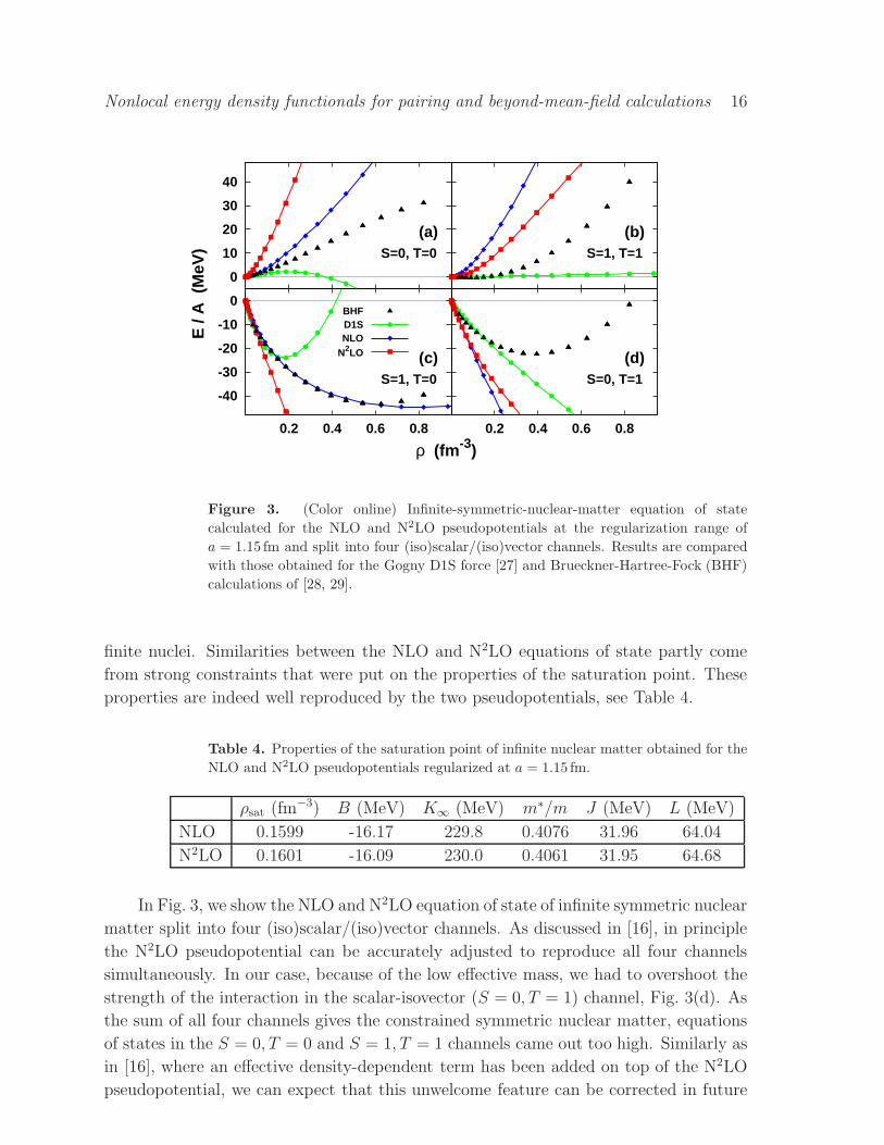
Figure 3. (Color online) Infinite-symmetric-nuclear-matter equation of state
calculated for the NLO and N2LO pseudopotentials at the regularization range of
a = 1.15 fm and split into four (iso)scalar/(iso)vector channels. Results are compared
with those obtained for the Gogny D1S force [27] and Brueckner-Hartree-Fock (BHF)
calculations of [28, 29].
finite nuclei. Similarities between the NLO and N2LO equations of state partly come
from strong constraints that were put on the properties of the saturation point. These
properties are indeed well reproduced by the two pseudopotentials, see Table 4.
Table 4. Properties of the saturation point of infinite nuclear matter obtained for the
NLO and N2LO pseudopotentials regularized at a = 1.15 fm.
ρsat (fm−3) B (MeV) K∞ (MeV) m∗/m J (MeV) L (MeV)
NLO 0.1599 -16.17 229.8 0.4076 31.96 64.04
N2LO 0.1601 -16.09 230.0 0.4061 31.95 64.68
In Fig. 3, we show the NLO and N2LO equation of state of infinite symmetric nuclear
matter split into four (iso)scalar/(iso)vector channels. As discussed in [16], in principle
the N2LO pseudopotential can be accurately adjusted to reproduce all four channels
simultaneously. In our case, because of the low effective mass, we had to overshoot the
strength of the interaction in the scalar-isovector (S = 0, T = 1) channel, Fig. 3(d). As
the sum of all four channels gives the constrained symmetric nuclear matter, equations
of states in the S = 0, T = 0 and S = 1, T = 1 channels came out too high. Similarly as
in [16], where an effective density-dependent term has been added on top of the N2LO
pseudopotential, we can expect that this unwelcome feature can be corrected in future

Nonlocal energy density functionals for pairing and beyond-mean-field calculations 17
implementations involving a three-body force.
5.2. Statistical error analysis
10-8
10-6
10-4
10-2
100
102
NLO
N2LO
2 4 6 8 10 12
Hessia
n-m
atr
ix e
igen
valu
es
Index of eigenvalue
Figure 4. (Color online) Eigenvalues of the Hessian matrices calculated from
the normalized penalty function for pseudopotentials at NLO and N2LO with the
regularization range of a = 1.15 fm.
For the two pseudopotentials built at NLO and N2LO with regularization range
a = 1.15 fm, we performed the analysis of statistical errors along the lines presented
in [25]. For that purpose, we considered the scaled penalty function χ2norm, for which we
calculated the Hessian matrix. Its eigenvalues are shown in Fig. 4. The total number
of eigenvalues corresponds to the number of parameters allowed to vary during the fit,
that is, to 9 for the pseudopotential at NLO and to 13 at N2LO.
Eigenvalues of the Hessian matrix are indicative of how well the penalty function is
constrained in those directions of the parameter space that are given by its eigenvectors.
From the gap between the second and third eigenvalue it clearly appears that,
irrespective of the order at which the pseudopotential is built, two such directions are
well constrained. Beyond this second eigenvalue, the eigenvalues decrease in a fairly
regular manner, and it is not possible to unambiguously define a dividing point between
relevant and irrelevant eigenvalues. Furthermore, we have checked that the directions
given by the eigenvectors of the Hessian matrix mix all the terms of the pseudopotential,
so that no coupling constant (for the parametrization we have adopted) can be removed
or frozen to get rid of a specific small eigenvalue.
The covariance matrix is the inverse of the Hessian matrix with a given number of
its eigenvalues kept [25]. Its average value, calculated for a vector of derivatives of a
given observable with respect to the parameters of the model, is called propagated error
of the observable. In Fig. 5, we show such propagated errors determined for several
observables in 120Sn and 166Er as functions of the number of largest eigenvalues kept in
the spectrum of the Hessian matrix.
Nonlocal energy density functionals for pairing and beyond-mean-field calculations 18
166ErN2LO
2 4 6 8 10 12
Number of kept eigenvalues
N2LO 120Sn
10-2
10-1
100
101
102
Pro
pa
gate
d e
rro
r in
%
NLO 166Er
10-2
10-1
100
2 4 6 8
NLO 120Sn
∆N ∆P E RP QP
(a) (b)
(c) (d)
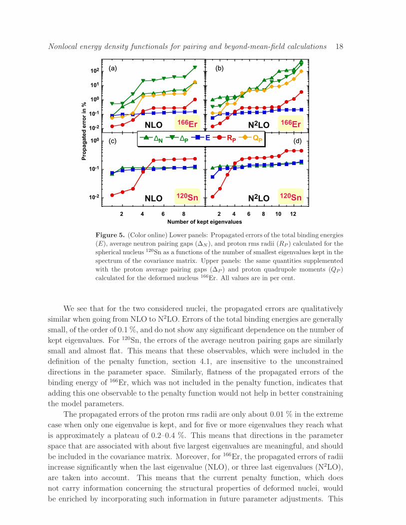
Figure 5. (Color online) Lower panels: Propagated errors of the total binding energies
(E), average neutron pairing gaps (∆N ), and proton rms radii (RP ) calculated for the
spherical nucleus 120Sn as a functions of the number of smallest eigenvalues kept in the
spectrum of the covariance matrix. Upper panels: the same quantities supplemented
with the proton average pairing gaps (∆P ) and proton quadrupole moments (QP )
calculated for the deformed nucleus 166Er. All values are in per cent.
We see that for the two considered nuclei, the propagated errors are qualitatively
similar when going from NLO to N2LO. Errors of the total binding energies are generally
small, of the order of 0.1 %, and do not show any significant dependence on the number of
kept eigenvalues. For 120Sn, the errors of the average neutron pairing gaps are similarly
small and almost flat. This means that these observables, which were included in the
definition of the penalty function, section 4.1, are insensitive to the unconstrained
directions in the parameter space. Similarly, flatness of the propagated errors of the
binding energy of 166Er, which was not included in the penalty function, indicates that
adding this one observable to the penalty function would not help in better constraining
the model parameters.
The propagated errors of the proton rms radii are only about 0.01 % in the extreme
case when only one eigenvalue is kept, and for five or more eigenvalues they reach what
is approximately a plateau of 0.2–0.4 %. This means that directions in the parameter
space that are associated with about five largest eigenvalues are meaningful, and should
be included in the covariance matrix. Moreover, for 166Er, the propagated errors of radii
increase significantly when the last eigenvalue (NLO), or three last eigenvalues (N2LO),
are taken into account. This means that the current penalty function, which does
not carry information concerning the structural properties of deformed nuclei, would
be enriched by incorporating such information in future parameter adjustments. This

Nonlocal energy density functionals for pairing and beyond-mean-field calculations 19
conclusion is substantiated by the propagated errors of quadrupole moments, which
increase from 0.1 % to even 100 %.
The main, and striking, difference between the results obtained for 120Sn and 166Er
concerns the average pairing gaps. As we already said, in 120Sn, the propagated errors
of the neutron gap are small and almost flat. However, in 166Er, one sees a clear
gradual increase of errors of pairing gaps with the number of kept eigenvalues. These
large propagated errors are likely associated with the sensitivity of gaps to deformation.
Indeed, changes of coupling constants induce changes of shape of the 166Er ground state,
and thus changes of its single-particle spectrum. This, in turn, can significantly modify
the average pairing gaps and lead to large calculated propagated errors. Altogether,
we conclude that adding to the penalty function data on spectroscopic properties of
deformed nuclei may be more interesting from the point of view of constraining the
model parameters than adding those related to their bulk properties like masses or
radii.
For the following part of this article, to calculate the propagated errors, we
chose to keep five largest eigenvalues of the Hessian matrices. This choice is based
on the observation that beyond this point, several propagated errors, like those of
radii, stop changing in a significant way. The corresponding covariance matrices are
provided in the supplemental material [URL]. In Table 3 we show statistical errors
of the coupling constants, which are equal to square roots of diagonal elements of
the covariance matrices [25]. Note that in Table 3 we show unrounded values of the
coupling constants, with several more digits beyond the statistically significant ones.
Nevertheless, performing calculations with properly rounded values does change results,
and significantly increases values of the penalty functions that move away from their
minima. These changes are, of course, within bounds of propagated errors and thus are
statistically insignificant, however, they also spoil smooth behaviour of observables and
parameters as functions of the regularization range a. Therefore, in all calculations we
recommend using the unrounded values of the coupling constants. Note also, that errors
of parameters serve to illustrate the overall uncertainty of parameters only, whereas
proper propagated errors of observables must be obtained by using the full covariance
matrices.
5.3. Finite nuclei
In Fig. 6, we show ground-state energies of selected spherical nuclei obtained for the
NLO and N2LO pseudopotentials regularized at a = 1.15 fm. In addition to nuclei that
were used to build the penalty function, results are shown for 44Ca, 90Zr, and 186Pb.
Apart from 48Ca, 120Sn, and 186Pb, the agreement of the calculated binding energies
with the experimental data is compatible with the calculated propagated errors. Large
deviations obtained for two outliers, 120Sn and 186Pb, can most probably be related to
the low effective mass and the resulting unrealistically small density of single-particle
states. This is illustrated in Fig. 7, where we show proton and neutron single-particle

Nonlocal energy density functionals for pairing and beyond-mean-field calculations 20
-4
0
4
8
12NLO
N2LO
40Ca
44Ca
48Ca
56Ni
78Ni
90Zr
100Sn
120Sn
132Sn
186Pb208
Pb
E -
EE
XP (
MeV
)
Figure 6. (Color online) Ground-state energies of selected spherical nuclei and their
propagated errors calculated for the NLO and N2LO pseudopotentials regularized at
a = 1.15 fm, relative to experiment. The two open-shell outliers 120Sn and 186Pb
(discussed in the text) are highlighted by the orange ellipse.
energies calculated in 208Pb in comparison with the empirical values taken from Ref. [30].
EXP NLO
-20
-15
-10
-5
0
5
3p1/23p3/22f5/21i13/2
2f7/2
1h9/2
3s1/2
2d3/2
1h11/2
2d5/2
1g7/2
N2LO (a)
Sin
gle
-pa
rtic
le e
nerg
ies (
Me
V)
Protons
-15
-10
-5
0
3p1/2
3p3/22f5/21i13/2
2f7/2
1h9/2
4s1/2
3d3/2
3d5/2
2g7/2
(b)
1j15/2
1i11/22g9/2
Neutrons
N2LONLOEXP
Figure 7. (Color online) Proton (left) and neutron (right) single-particle energies
calculated in 208Pb in comparison with the empirical values taken from Ref. [30]
Note that states appearing at positive energies rather correspond to single-particle
resonanses estimated by using the finite harmonic-oscillator basis.
As can be seen in Figs. 6 and 7, results obtained for both pseudopotentials are
fairly similar, and we do not see any significant improvement when going from NLO
to N2LO. This is also visible in Table 2, where the decrease of the penalty function is
Nonlocal energy density functionals for pairing and beyond-mean-field calculations 21
mostly related to the improvement of nuclear-matter properties.
-4
-2
0
2
4
6
8 NLO
N2LO
44Ca
44Cr46Ti
54Cr150Ce
160Gd166Er
208Pb252Cf
E -
EG
og
ny
D1
S (
MeV
)
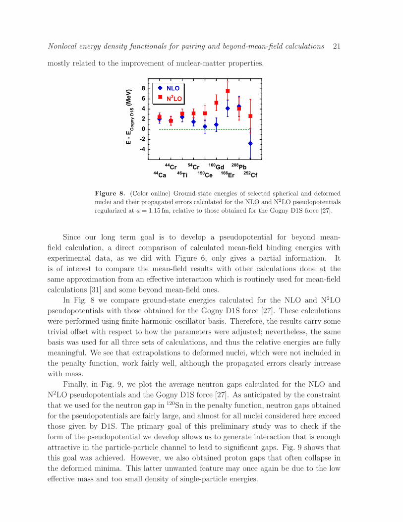
Figure 8. (Color online) Ground-state energies of selected spherical and deformed
nuclei and their propagated errors calculated for the NLO and N2LO pseudopotentials
regularized at a = 1.15 fm, relative to those obtained for the Gogny D1S force [27].
Since our long term goal is to develop a pseudopotential for beyond mean-
field calculation, a direct comparison of calculated mean-field binding energies with
experimental data, as we did with Figure 6, only gives a partial information. It
is of interest to compare the mean-field results with other calculations done at the
same approximation from an effective interaction which is routinely used for mean-field
calculations [31] and some beyond mean-field ones.
In Fig. 8 we compare ground-state energies calculated for the NLO and N2LO
pseudopotentials with those obtained for the Gogny D1S force [27]. These calculations
were performed using finite harmonic-oscillator basis. Therefore, the results carry some
trivial offset with respect to how the parameters were adjusted; nevertheless, the same
basis was used for all three sets of calculations, and thus the relative energies are fully
meaningful. We see that extrapolations to deformed nuclei, which were not included in
the penalty function, work fairly well, although the propagated errors clearly increase
with mass.
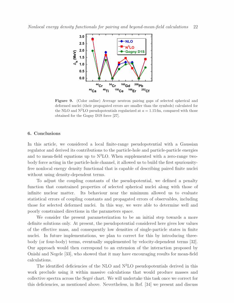
Finally, in Fig. 9, we plot the average neutron gaps calculated for the NLO and
N2LO pseudopotentials and the Gogny D1S force [27]. As anticipated by the constraint
that we used for the neutron gap in 120Sn in the penalty function, neutron gaps obtained
for the pseudopotentials are fairly large, and almost for all nuclei considered here exceed
those given by D1S. The primary goal of this preliminary study was to check if the
form of the pseudopotential we develop allows us to generate interaction that is enough
attractive in the particle-particle channel to lead to significant gaps. Fig. 9 shows that
this goal was achieved. However, we also obtained proton gaps that often collapse in
the deformed minima. This latter unwanted feature may once again be due to the low
effective mass and too small density of single-particle energies.
Nonlocal energy density functionals for pairing and beyond-mean-field calculations 22
0.0
0.5
1.0
1.5
2.0
2.5
3.0
NLO
N2LO
Gogny D1S
44Ca
44Cr
46Ti
54Cr
150Ce
160Gd
166Er
208Pb
252Cf
∆ N (
MeV
)
Figure 9. (Color online) Average neutron pairing gaps of selected spherical and
deformed nuclei (their propagated errors are smaller than the symbols) calculated for
the NLO and N2LO pseudopotentials regularized at a = 1.15 fm, compared with those
obtained for the Gogny D1S force [27].
6. Conclusions
In this article, we considered a local finite-range pseudopotential with a Gaussian
regulator and derived its contributions to the particle-hole and particle-particle energies
and to mean-field equations up to N2LO. When supplemented with a zero-range two-
body force acting in the particle-hole channel, it allowed us to build the first spuriousity-
free nonlocal energy density functional that is capable of describing paired finite nuclei
without using density-dependent terms.
To adjust the coupling constants of the pseudopotential, we defined a penalty
function that constrained properties of selected spherical nuclei along with those of
infinite nuclear matter. Its behaviour near the minimum allowed us to evaluate
statistical errors of coupling constants and propagated errors of observables, including
those for selected deformed nuclei. In this way, we were able to determine well and
poorly constrained directions in the parameters space.
We consider the present parameterization to be an initial step towards a more
definite solutions only. At present, the pseudopotential considered here gives low values
of the effective mass, and consequently low densities of single-particle states in finite
nuclei. In future implementations, we plan to correct for this by introducing three-
body (or four-body) terms, eventually supplemented by velocity-dependent terms [32].
Our approach would then correspond to an extension of the interaction proposed by
Onishi and Negele [33], who showed that it may have encouraging results for mean-field
calculations.
The identified deficiencies of the NLO and N2LO pseudopotentials derived in this
work preclude using it within massive calculations that would produce masses and
collective spectra across the Segre chart. We will undertake this task once we correct for
this deficiencies, as mentioned above. Nevertheless, in Ref. [34] we present and discuss
Nonlocal energy density functionals for pairing and beyond-mean-field calculations 23
results of calculations performed in semi-magic nuclei, and we refer the Reader to this
publication for further information.
Acknowledgments
We wish to thank Marcello Baldo for providing us with his results from Brueckner-
Hartree-Fock calculations of infinite nuclear matter and Michael Bender for a careful
reading of this manuscript and helpful comments. K.B. thanks Tomas Rodriguez
and Nicolas Schunck for useful discussions and benchmark calculations during the
development of the code finres4. This work was supported by the Academy of
Finland and University of Jyvaskyla within the FIDIPRO program, by the Royal
Society and Newton Fund under the Newton International Fellowship scheme, by the
CNRS/IN2P3 through PICS No. 6949, by the Polish National Science Center under
Contract No. 2012/07/B/ST2/03907, and by the Academy of Finland under the Centre
of Excellence Program 20122017 (Nuclear and Accelerator-Based Physics Program at
JYFL). We acknowledge the CSC-IT Center for Science Ltd., Finland, for the allocation
of computational resources.
References
[1] Skyrme T H R 1956 Philosophical Magazine 1 1043–1054
[2] Skyrme T H R 1959 Nuclear Physics 9 615 – 634 ISSN 0029-5582 URL
http://www.sciencedirect.com/science/article/pii/0029558258903456
[3] Decharge J and Gogny D 1980 Phys. Rev. C 21(4) 1568–1593 URL
http://link.aps.org/doi/10.1103/PhysRevC.21.1568
[4] Dobaczewski J, Stoitsov M V, Nazarewicz W and Reinhard P G 2007 Phys. Rev. C 76(5) 054315
URL http://link.aps.org/doi/10.1103/PhysRevC.76.054315
[5] Anguiano M, Egido J and Robledo L 2001 Nuclear Physics A 696 467 – 493 ISSN 0375-9474 URL
http://www.sciencedirect.com/science/article/pii/S0375947401012192
[6] Bender M, Duguet T and Lacroix D 2009 Phys. Rev. C 79(4) 044319 URL
http://link.aps.org/doi/10.1103/PhysRevC.79.044319
[7] Tarpanov D, Toivanen J, Dobaczewski J and Carlsson B G 2014 Phys. Rev. C 89(1) 014307 URL
http://link.aps.org/doi/10.1103/PhysRevC.89.014307
[8] Skyrme T H R 1957 A nuclear pseudo-potential Proc. of the Rehovot conference on nuclear
structure ed Lipkin H (North-Holland, Amsterdam, 1958) pp 20 – 25
[9] Raimondi F, Bennaceur K and Dobaczewski J 2014 Journal of Physics G: Nuclear and Particle
Physics 41 055112 URL http://stacks.iop.org/0954-3899/41/i=5/a=055112
[10] Dobaczewski J 2016 Journal of Physics G: Nuclear and Particle Physics 43 04LT01 URL
http://stacks.iop.org/0954-3899/43/i=4/a=04LT01
[11] Carlsson B G, Dobaczewski J and Kortelainen M 2008 Phys. Rev. C 78(4) 044326 URL
http://link.aps.org/doi/10.1103/PhysRevC.78.044326
[12] Raimondi F, Carlsson B G and Dobaczewski J 2011 Phys. Rev. C 83(5) 054311 URL
http://link.aps.org/doi/10.1103/PhysRevC.83.054311
[13] Dobaczewski J, Bennaceur K and Raimondi F 2012 Journal of Physics G: Nuclear and Particle
Physics 39 125103 URL http://stacks.iop.org/0954-3899/39/i=12/a=125103
[14] Sadoudi J, Bender M, Bennaceur K, Davesne D, Jodon R and Duguet T 2013 Phys. Scr. T154
014013 URL http://stacks.iop.org/1402-4896/2013/i=T154/a=014013

Nonlocal energy density functionals for pairing and beyond-mean-field calculations 24
[15] Bennaceur, K, Dobaczewski, J and Raimondi, F 2014 EPJ Web of Conferences 66 02031 URL
http://dx.doi.org/10.1051/epjconf/20146602031
[16] Davesne D, Navarro J, Becker P, Jodon R, Meyer J and Pastore A 2015 Phys. Rev. C 91(6) 064303
URL http://link.aps.org/doi/10.1103/PhysRevC.91.064303
[17] Perlinska E, Rohozinski S G, Dobaczewski J and Nazarewicz W 2004 Phys. Rev. C 69(1) 014316
URL http://link.aps.org/doi/10.1103/PhysRevC.69.014316
[18] Bennaceur K et al 2017, to be submitted to Computer Physics Communications
[19] Hooverman R 1972 Nuclear Physics A 189 155 – 160 ISSN 0375-9474 URL
http://www.sciencedirect.com/science/article/pii/0375947472906501
[20] Dobaczewski J et al 2017, to be submitted to Computer Physics Communications
[21] Schunck N, Dobaczewski J, McDonnell J, Satua W, Sheikh J, Staszczak A, Stoitsov M and
Toivanen P 2012 Computer Physics Communications 183 166 – 192 ISSN 0010-4655 URL
http://www.sciencedirect.com/science/article/pii/S0010465511002852
[22] Schunck N, Dobaczewski J, Satu la W, Baczyk P, Dudek J, Gao Y, Konieczka M, Sato K,
Shi Y, Wang X B and Werner T R 2017 Submitted to Computer Physics Communications,
arXiv:1612.05314v2 URL http://arxiv.org/abs/1612.05314v2
[23] JS Bell and THR Skyrme Phil Mag 1, 1055 (1956)
[24] M Bender, K Rutz, P-G Reinhard and JA Maruhn 2000 Eur. Phys. J. A 7 467–478 URL
http://dx.doi.org/epja/v7/p467(epja219)
[25] Dobaczewski J, Nazarewicz W and Reinhard P G 2014 Journal of Physics G: Nuclear and Particle
Physics 41 074001 URL http://stacks.iop.org/0954-3899/41/i=7/a=074001
[26] Hellemans V, Pastore A, Duguet T, Bennaceur K, Davesne D, Meyer J,
Bender M and Heenen P H 2013 Phys. Rev. C 88(6) 064323 URL
http://link.aps.org/doi/10.1103/PhysRevC.88.064323
[27] Berger J, Girod M and Gogny D 1991 Computer Physics Communications 63 365 – 374 ISSN
0010-4655 URL http://www.sciencedirect.com/science/article/pii/001046559190263K
[28] Baldo M, Bombaci I and Burgio G F 1997 Astron. Astrophys. 328 274–282
[29] Baldo M private communication
[30] Schwierz N, Wiedenhover I and Volya A 2007 arXiv:0709.3525 URL
http://arxiv.org/abs/0709.3525
[31] Hilaire S and Girod M URL http://www-phynu.cea.fr/science_en_ligne/carte_potentiels_\microscopiques/cart
[32] Sadoudi J, Duguet T, Meyer J and Bender M 2013 Phys. Rev. C 88(6) 064326 URL
http://link.aps.org/doi/10.1103/PhysRevC.88.064326
[33] Onishi N and Negele J 1978 Nuclear Physics A 301 336 – 348 ISSN 0375-9474 URL
http://www.sciencedirect.com/science/article/pii/037594747890266X
[34] Bennaceur K, Dobaczewski J and Gao Y 2017 arXiv:1701.08062 URL
http://arxiv.org/abs/1701.08062