engineering Costs and subduction E~~~omi~s, 20 ( 1990) 8 l-9 1 Elsevier

NONLlNEAR MULTIPRODUCT CVP ANALYSIS WITH O-1 MIXED INTEGER PROGRAMMING

Wen-Hsien Tsai Depa~ment of Business Administration, National Central University, Chung-ii, Taiwan

Tsong-Ming Lin Department of Industrial Management, National Taiwan Institute of Technology, Taipei, Taiwan

ABSTRACT

This paper presents O-l Mixed Integer Pro- gramming model for the nonlinear multiprod- uct Cost- Volume-Profit analysis, which re- laxes the assumptions of linear revenue-cost functions and constant~xed cost. In this model, nonlinear revenue and cost functions are ap- proximated by piecewise linear functions, and the joint fixed cost function is represented by a

step-increment function. With these features, the required capacity level and the optimal product mix could be determined simultaneously. A hy- pathetical example, illustrating the model, is presented together with the profit-maximiza- tion solution, the breakeven solution, and the target-profit solutions.

1. INTRODUCTION

Cost-Volume-Profit (CVP) analysis is a technique used to analyze the impact on prof- its of various decisions that affect revenues and costs. One of the limiting assumptions of tra- ditional CVP analysis is that there is only one product or a constant mix of products. In 196 1, Jaedicke [ 1 ] applied Linear Programming (LP) techniques to construct a CVP model, called a “Product Mix” model in many man- agement accounting or LP texts, which could aid management to determine the optimal product mix, maximizing total profit under some limits (constraints} to production or sales in the case of multiproduct firrn8. By sen- sitivity analysis techniques of LP, manage- ment could evaluate the impact on profits or

product mixes of changing product prices, unit variable costs, resource restrictions, or combi- nations of these factors [ 21. This model could be slightly modified into a linear goal pro- gramming model, which could determine the product mix under the breakeven condition or specific profit levels [ 3 1.

LP applications have extensively appeared in the accounting literature; for instance, Hartley [ 4 ] applies LP techniques to the joint product decision problem, which is another kind of multiproduct CVP analysis problem. How- ever, the LP approach of CVP analysis still re- tains the following two simplifying assump- tions: ( 1) unit prices and unit variable costs are constant, i.e., the contribution functions are linear within the relevant range, and (2) the fixed cost, which is not divided into specific

0167-I 88X/90/$03.50 0 1990 - Elsevier Science Publishers B.V.

82

fixed cost and joint fixed cost, is constant within the relevant range.

To relax these two assumptions, Sheshai et al. [ 5 ] utilize Integer Goal Programming (which is O-l Mixed Integer Programming strictly speaking) to construct a nonlinear CVP model which expresses each product’s contri- bution as a piecewise linear function and spe- cific fixed cost as a step-increment function. Nevertheless, the model Sheshai et al. present needs the special observance of the association between the contribution function and the varying levels of fixed costs. This special ob- servance becomes unwieldy when there are many kinds of products in the model.

The purpose of this paper is to present a sim- pler nonlinear CVP model with 0- 1 Mixed In- teger Programming (0- 1 MIP ) , which relaxes the assumptions mentioned above and consid- ers the discrete capacity extensions. In Section 2, the general form of the nonlinear CVP model is explained in detail; in Section 3, some solu- tion techniques in the literature are discussed; in Section 4, an illustrative example is pre- sented together with the profit-maximization solution, the breakeven solution, and the tar- get-profit solutions.

2. NONLINEAR CVP MODEL

2.1 Assumptions

The nonlinear CVP model presented in this paper is subject to the following assumptions:

( 1) In a multiproduct manufacturing firm, total cost is divided into total joint fixed cost, total direct material cost, total direct labor cost, and total other cost.

( 2 ) Joint fixed cost can be measured by ma- chine hours, and is assumed to be a step-incre- ment function, i.e., the acquisition of machine hours comes in indivisible chunks.

(3) The cost functions of total direct mate- rial and total direct labor are piecewise linear functions, which approximate the nonlinear

cost behaviors, due to quantity discount and higher overtime wage rate.

(4) For each product, “other cost” is the sum of the cost of production and the expenses of administration and marketing except direct material and direct labor costs, and its behav- ior is a mixed cost pattern.

(5) For each product, its revenue is as- sumed to be a piecewise linear function which approximates the nonlinear revenue behavior due to the law of diminishing return.

2.2 Presentation of a piecewise linear function

In real life the revenue and cost functions are nonlinear functions, which are approximated by piecewise linear functions in this model. Figure 1 shows an illustration of the piecewise linear function. In Fig. 1, the piecewise linear curve is composed of k successive segments, each with a different slope, indicating differ- ent marginal revenue or marginal cost over a different range of volume. Points labeled as P ,,...,Pk are called “bend points” in this paper, whose coordinates are ( vl,Y, ) ,..., ( I& Yk), respectively. Let si be the slope of the ith seg- ment; then the formula for calculating Yi is

where YO= 0 and I’,= 0. Besides, note that V, is the upper limit of volume. The function value and the associated constraints for this il- lustration are as follows: Function value:

YE* 2 y,aj (1.1) j=l

Constraints:

&J--s, co

,I,-6,-S,+, <O j=I,...,k-1

&-&GO

c:=J, = 1

c:,lSj= 1

(1.2)

( 1:.3 1

(1.4)

(1.5)

(1.6)

Fig. I. A piecewise Iinear function.

v-~;~lv,a,=o

aj=o,l j= l,..., k; LjaO j=O,...,k

(1.7)

The term ( 1.1) will be positive for revenue and negative for cost. (6,,&,...,&) is an SOS1 set of O-l variables within which exactly one variable must be nonzero; (&,121,...,&) is an SOS2 set of nonnegative variables within which at most two adjacent variables, in the ordering given to the set, can be nonzero [ 6,7 1. By eqn. ( 1.5 ) , we know that at most two adjacent non- zero /zj”s sum up to 1. Thus, the values of Y and V will be the linear combinations of two adja- cent Yj’s and two adjacent Vj’s, respectively, by eqns. (1.1) and (1.7). For example, if (r3= 1, then /12 and a 3 sum up to 1, other n;s are zero, Y is equal to Y2A2 + Yd3, and V is equal to v,n,+ v,n,.

2.3 Description of the model

The complete model this paper presents is as follows:

(2.1)

Constraints:

for i= l,...,y1

cfa-ei, ~0

ajj-9,-e,,+, ~0 j=l,_.., k,-1

ffiktr - @rki, 6 0

C$&jj = 1

c;:,e,j= i

x~-~$,uijaij=o

Xi - uik,,& Q 0

f3q =O,l i= l,..., ?Z;j= I,...) k,+ <i =O,l i=l,...,n %j =Opl s= m,h; j= l,...,k, f!Lj =O,l j=O,...,g other variables are nonnegative.

83

(2.2)

(2.3)

(2.4)

(2.5)

(2.6)

(2.7)

(2.8)

(2.9)

(2.10)

(2.11)

(2.12)

(2.13)

(2.14)

(2.15)

(2.16)

Equation (2.1) represents the total profit function 2, and eqns. (2.2)-(2.16) are the constr~nts associated with revenue functions and various cost functions. The discussion which follows explains the elements in the model.

23.1 Total revenue

Assume that there are n products and that the revenue function of each product is a pie- cewise linear function due to price reduction for additional sales. For product i, let the num- ber of units of product i be Xi and let the coor- dinates of the kir bend points of its revenue

84

function be (U,, Rij, j= l,..., ki,. Thus, the UP- per limit of the volume of product i is Uik,,.

To express the associated constraints of the piecewise linear revenue function, we intro- duce some nonnegative variables aii and some O-l variables 8,, j= I ,..., ,r, k * these constraints are represented by eqns. (2.2)-(2.7). Just like the description in Section 2.2, (aiO, ai, ,..., (Yiki,) is an SOS2 set, (&,Biz ,..., &,,) is an SOS1 set, the revenue of product i is 27; IR,o, and the number of units of product i is Xf:, U+Q. Because we have y1 products, there are y1 sets of eqns. (2.2)-(2.7), and the total revenue is C:= 1 1:: IRuaij as shown in the first term of eqn. (2.1).

2.3.2 Total direct material cost

This model assumes that all products utilize the same direct material, whose cost function is a piecewise linear function due to quantity discount. Let the requirement of direct mate- rial for one unit of product i be a,i units and the coordinates of the km bend points of the total direct material cost function be ( W’mj,Cmj) J= 1 ,..., k,. Thus u/nzk, is the avail- able volume of direct material.

To express the associated constraints of the piecewise linear function of total direct mate- rial cost, we introduce some nonnegative vari- ables /3mj and some O-l variables tlt,ij= 1 ,...,k,; these constraints are represented by eqns. (2.9)-(2,14), where the subscript s is re- placed by m. Just like the description in Sec- tion 2.2., (/?m,,fimZ ,..., /Imk,) is an SOS2 set, (%nlJlm2,*.*9 &&,, ) is an SOS 1 set, the total di- rect material cost is Cik_“lC,,$mj, shown in the second term of eqn. (2.1) and the total re- quirement of direct material is Z$:, Wmjfimj, as in eqn. (2.14).

2.3.3 Total direct labor cost

This model assumes that the total direct la- bor cost function is also a piecewise linear function due to overtime premium. Let the re-

quirement of direct labor for one unit of prod- uct i be ahi hours. The representation of the to- tal direct labor cost function, shown in the third term of eqn. (2.1) and eqns. (2.7)-(2.14), is the same as that of the total direct material cost function, except the subscript s is replaced by h. Thus, total direct labor cost isC:L, C/gjphj and total requirement of direct labor is 1;; ~‘u/;ljfi~~

2.3.4 Total other cost

For each product, other cost is assumed to be the sum of the cost of production and the expenses of administration and marketing, ex- cluding direct material cost and direct labor cost. Other cost includes the specitic fixed cost for each product, so it can be divided into vari- able and fixed components. This model as- sumes its behavior is a mixed cost pattern and can be estimated by statistical regression anal- ysis. The representation of total other cost is shown in eqn. (2.8 ) and the forth term of eqn. (2.1), where Foi stands for the specific fixed cost for product i and Coi is the increment of other cost for producing one more unit of product i, The specific fixed cost Foi can be avoided if we decide not to produce product i. Here, O-l variables &,i= l,...,n, are introduced to express this cost phenomenon. When & = 0, it means that Xi=0 by eqn. (2.8) and that Foi and Coi vanish from the objective function.

2.3.5 Total joint fixed cost

Joint fixed cost is the capacity cost incurred for the common benefit of all products. It usu- ally cannot be specifically identified with a particular product. However, this model as- sumes that this kind of capacity cost can be measured by the machine hours in a machine- intensive manufactu~ng company and that its cost function is a ste~increment fun~ion as shown in Fig. 2. This cost behavior pattern means the capacity extensions in finite jumps, e.g., buying in whole new machines when pro- duction is expanded beyond a certain level.

85

The joint fixed cost is F,, under the current capacity bO. If the capacity is successively ex- panded to b b 1, 2 ,..., bg, then the joint fixed cost increases to F 1, F 2 ,..., Fg, respectively. Thus, the joint fixed cost function can be expressed by eqns. (2.15), (2.16) and the last term of eqn. (2.1)) where U,i is the requirement of machine hours for producing one unit of product i and (~,~r,...,~ug) is an SOS1 set of O-l variables. When pj= 1, we know that the capacity needs to be expanded to thejth level, i.e., bj machine hours.

2.4 Remarks

For the model we present, there are some re- marks which should be mentioned here. First of all, the piecewise linear function can ap- proximate nonlinear revenue or cost behavior

Ez! I Fg t----- ;

Fig. 2. Total joint fixed cost function.

$zk E

- Real function

--- - - piecewise tinear appmximat’bn

lblume Fig. 3. An illustration of a piecewise linear approximation.

in real world which is estimated either by en- gineering analysis or by curve-fitting tech- nique. For example, the solid curve in Fig. 3 can be approximated by the dotted lines com- posed of four segments. If the nonlinear curve is approximated by more segments, this will improve the accuracy of the approximation. It, nevertheless, will increase the numbers of vari- ables and constraints.

Second, one can divide total cost into more items than this model does. Our model has demonstrated the mathematical expressions of various patterns of cost behavior, so the addi- tional cost items can be represented in terms of a linear or nonlinear function according to their behaviors.

Third, product mix solutions are not always in integer units. If an integer solution is re- quired, then we should let X, be integer and solve the problem by another kind of 0- 1 MIP.

Finally, note that the model should be slightly modi fed in order to acquire the break- even solution or target-profit solutions. The model described in Section 2.3 is the profit- maximization model, where the objective function .is to maximize total profit whose function is shown in eqn. (2.1) . To acquire the product mix solution under specific profit level Z,, the following constraint should be added:

Z-e++e-=Z

where Z is the total profit function, and e+ and e- are, respectively, positive and negative de- viations from Z,. Thus the objective function is to minimize e+ +e-. In addition, let Z, be zero, then the breakeven solution could be acquired.

3. SOLUTION TECHNIQUES

The nonlinear CVP model presented in this paper is a 0- 1 MIP model, which involves 0- 1 variables and nonnegative variables. There are three 0- 1 implicit enumeration algorithms for solving the O-l MIP model: the penalty algo- rithm [ 8 1, the partitioning algorithm [ 9 1, and

86

the modified partitioning algorithm [ 10 J. A fourth method is the Branch-and-Bound {B&B) algorithm [ 111, In fact, the O-l im- plicit enumeration algorithm can be classified as a B&B method. The B&B method has thus far proven to be the most reliable among the various methods for solving the O-l MIP model, and all commercial integer program- ming codes use this method.

The nonlinear CVP model employs special order sets of variables, SOS 1 and SOS2 sets, to approximate nonlinear functions by piecewise linear functions. The way in which the B&B al- gorithm can be modified to deal with SOS 1 and SOS2 sets is described in [ 6, 12 1. This kind of approximation will increase the size of the model as well as the computational difficulty. However, Martin and Schrage [ 13 ] have de- veloped a subset coefficient reduction method for generating cuts to tighten the O-l MIP model prior to implementing an LP based B&B algorithm, in order to reduce the size of the coefficients of the 0- 1 variables.

Although the various methods mentioned above can be used to solve the nonlinear CVP model, it will take a long time for practicians to convert the algorithms into computer codes. Fortunately, several ready-made computer codes f 14, 15 1, e.g., the software LINDO [ 16, 17 1, are available to solve the nonlinear CVP model. Hence, the practicians could focus their attentions on model building rather than programming.

4. ILLUSTRATION

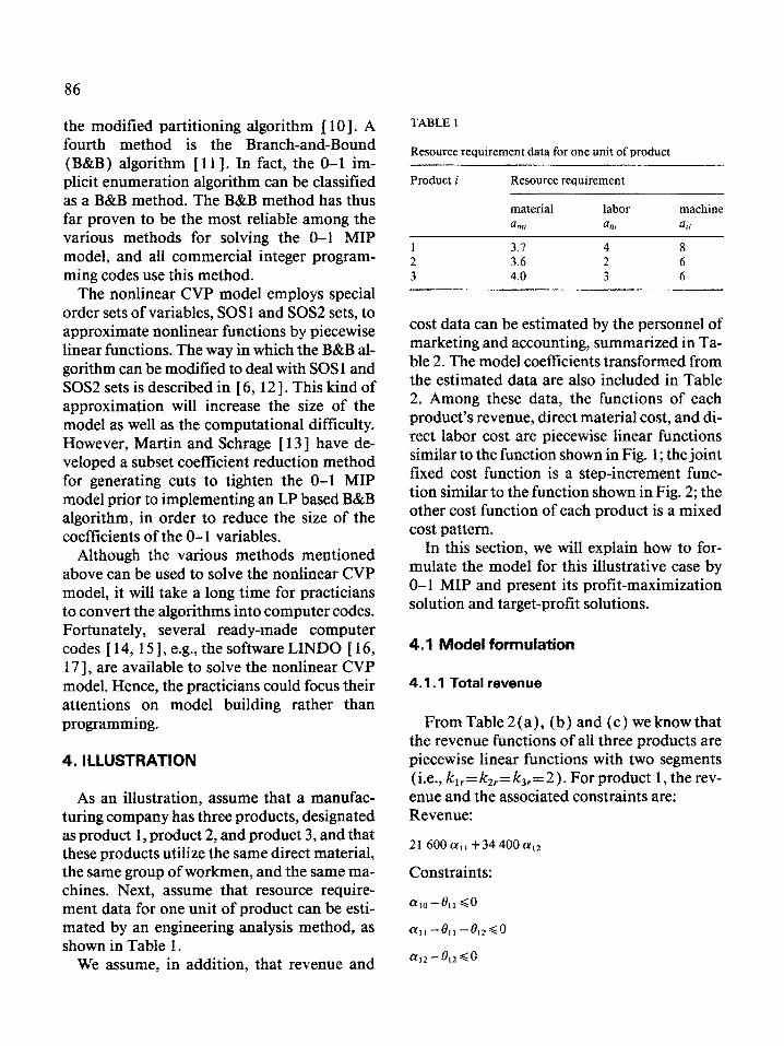
As an illustration, assume that a manufac- turing company has three products, designated as product 1, product 2, and product 3, and that these products utilize the same direct material, the same group of workmen, and the same ma- chines. Next, assume that resource require- ment data for one unit of product can be esti- mated by an engineering analysis method, as shown in Table 1.

We assume, in addition, that revenue and

TABLE 1

Resource requirement data for one unit of product

Product i Resource requirement

material labor am, ahr

machine

ali

1 3.7 4 8 2 3.6 2 6 3 4.0 3 6

cost data can be estimated by the personnel of marketing and accounting, summarized in Ta- ble 2. The model coefficients transformed from the estimated data are also included in Table 2. Among these data, the functions of each product’s revenue, direct material cost, and di- rect labor cost are piecewise linear functions similar to the function shown in Fig. 1; the joint fixed cost function is a step-increment func- tion similar to the function shown in Fig. 2; the other cost function of each product is a mixed cost pattern.

In this section, we will explain how to for- mulate the model for this illustrative case by O-l MIP and present its profit-maximization solution and target-profit solutions.

4.1 Model formulation

4.1 .l Total revenue

From Table 2(a), (b) and (c) we know that the revenue functions of all three products are piecewise linear functions with two segments (i.e., kl,= kzr= k,,=2). For product 1, the rev- enue and the associated constraints are: Revenue:

21 6OOff,,+34400~,*

Constraints:

87

TABLE 2 a,*Sal, +a,,l=1

e,, f&2= 1

~~-60o~,~-loooff,~=o.

Next, the analogous expressions for product 2 are: Revenue:

Constraints:

Revenue and cost data of illustrative case

(a f Revenue data of product 1 (i = 1)

j volume marginal model coeff. revenue ($ )

fJtj Rtj ($)

1 l- 600 36 600 21 600 2 601-1000 32 1000 34 400

( b ) R~vmzre data o~~~~~~t Z fi = .?,I

j v&me marginal model coeff. revenue ($ )

u2j hj ($)

1 l-600 28 600 16 800 2 601-900 25 900 24 300

( c ) ~~v~~ue data u_f product 3 {i = 3)

i volume marginal model coeff. revenue ($ )

hi R3j ($)

1 I-500 30 2 501-800 26

(d ) D~FCTC~ ~~t~~ia~ cmt data

.i volume marginal cost ($)

500 15 000 800 23 400

model coeff.

w,i c, ($)

1 l- 5000 1.0 2 5001- 8000 0.8 3 8001-10000 0.7

(e ) Direct Labor cosi data

i volume marginal cost ($)

5 000 5000 8 000 7400

10000 8800

model coeff,

bv,, chj ($1

1 l-4000 2 2 4~0~-6~00 3

( f ) U&r ~osb data Product i components

4of.H 8 000 6000 14 000

fixed variable F,, (S) coi ($1

1 1800 6 2 2100 5 3 2200 4

(g) Joint fixed cost data

i increment increment model coeff. of machine of joint hOtES fixed cost ($1 bj Fi ($1

0 8000 8000 8000 8 000 1 2000 2000 10 000 10 000 2 4000 4000 12 000 12 000

a20-021 60

a21 - u 7.1 -022go

Q 22-@22<0

cr,,+-cl!21 +a22=1

$2, +t?22=1

x2 - 600 CqYj - 900 A!*2 =a

Finally, the analogous expressions for product 3 are: Revenue:

15 000 cY3, f 23 400 (Y32

am-&, 60

4.12 Total direct material cost

From Table 2 (d ), we know that the direct material cost function is a piecewise linear function with three segments (i.e., k,= 3). It is because of quantity discount; the marginal cost of material is $1 under 5000 units, $0.8 between 5001 and 8000 units, and $0.7 be- tween 8001 and 10 000 units. Furthermore, the

88

material requirements to produce one unit of product 1, product 2 and product 3 are 3.7, 3.6 and 4 units, respectively. Therefore, total di- rect material cost and the associated con- straints are: Total direct material cost:

Pho+Phl +Ph2= 1

vhl+nz2=1

4X, •k 2X, +3X, - 4000 j?,,, - 6000 /?,,I = 0.

4.1.4 Total other cost

5ooop,,+74oop,,+88oop,~

Constraints:

Lo-)l???, GO

am, -)lml -%&GO

Pm2-)Im2-%?3~O

Pd--G13<0

Pmo+Pml +Dm2+Pm3=1

%nl+%72+%n3=1

3.7X, +3.6X2 +4X, - 5000 /3,,,,

Other cost data of the three products are shown in Table 2 ( f ). Total other cost and the associated constraints are: Total other cost:

1800~,+6X,+2100~,+5X,+2200~~+4X,

Constraints:

x,-1000~,<0

x,-!?oo<~,<o

xx-800&<0.

4.1.5 Joint fixed cost

From Table 2 (g), we know that the current capacity is 8000 machine hours and that it can be expanded to 10 000 or 12 000 machine hours with the additional cost of $2000 or $4000. Besides, the machine hours require- ments to produce one unit of product 1, prod- uct 2 and product 3 are 8, 6 and 6 hours, re- spectively. Thus, total joint fixed cost and the associated constraints are: Total joint fixed cost:

8000~+10000,u,+12000p2

Constraints:

4.1.3 Total direct labor cost

From Table 2 (e), we know that the direct labor cost function is a piecewise linear func- tion with two segments (i.e., kh=2). Here, we assume that this company executes the time- work wage system; the available normal labor hours are 4000 hours with the hourly rate of $2, and the available overtime labor hours are 2000 hours with the hourly rate of $3. More- over, the labor requirements to produce one unit of product 1, product 2 and product 3 are 4, 3 and 3 hours, respectively. Thus, total di- rect labor cost and the associated constraints are: Total direct labor cost:

4.2 Solution 8000/$, , + 14 000 phz

Constraints:

ph2-&2<0

4.2.1 Profit-maximization solution

If the goal of management is to achieve the maximum profit, then the objective function is to maximize the following function:

Z= (total revenue) - (total direct material cost)

- (total direct labor cost)

- (total other cost) - (total joint fixed cost)

=(21 600~,,+34400~~,~+16800a~,

$24 300 CY** + 15 000 LYE, +23 400 czj2)

- (SOOOP,, +7400/I,,,* +8800/I,,)

- (8000/3h, + 14 OOO&)

-(1800~,+6X,+2100~,+5X,+2200~,+4X,)

-(8000p0+10000p~+12000,uL2)

We solve this O-l MIP problem by software LINDO and obtain the following optimal solution:

x, =450, &=I, &,=l, k=O,

X,=600, 52= 1, 021 =O, &2= 1,

X, = 800, &=l, e,,=o, k= 1,

cu10=0.25, (~,,=0.75, CY,~=O, k=O,

ff20 = 0, a,,=]. ~22=0, A=&

a30=0, ~3,=0, a32= 1, P2= 1,

~,,,o=0,&,=0.325,~m2=0.675,~,,,~=0,~m~=0,~m2=1,

?m3=O,Pho=O,Ph,=0.3,Ph2=0.7, %,l=o, qh2=l.

Accordingly, the optimal product mix is (X1,X,$,= (450,600,800), which requires 7025 x (450.3.7+600-3.6+800-4) units of material, 6000x (450.4+600*3+800*3) la- bor hours, and 12 000x (450.8+600*6 + 800.6) machine hours. Total revenue, total direct material cost, total direct labor cost, to- tal other cost, and total joint fixed cost are $56 400, $6620, $12 200, $15 000, and $12 000 respectively, calculated by the expres- sions mentioned above. Thus, total profit is $10 580.

4.2.2 Target-profit solutions

As mentioned previously, the following con- straint should be added in order to acquire the product mix solution under specific profit level zc:

Z-e++e-=Z,,

and the objective function is changed into minimizing e + + e-. The product mix solu- tions under various target profit levels for the illustrative case are shown in Table 3. The breakeven product mix (when Z,=O) is

89

TABLE 3

Target-profit solutions

Target Product mix (in units) deviations profit

ZC ($) XI x2 x3 e+ e-

0 535.5192 0 0 0 0 1 000 262.2951 0 800 0 0 2 000 316.9399 0 800 0 0 3 000 371.5847 0 800 0 0 4 000 582.5137 600 0 0 0 5 000 545.4546 0 745.4545 0 0 6 000 156.2842 600 500 0 0 7 000 0 600 785.6757 0 0 8 000 0 660.0610 800 0 0 9 000 0 736.2805 800 0 0

10 000 787.3187 900 0 0 0 10 580 450 600 800 0 0 11000 450 600 800 0 420 12 000 450 600 800 0 1420

(X,,X,,X,) = (535.5192,0,0); it means that only product 1 is produced. From Table 5, we see that the achievable maximum profit is $10 580, above which the negative deviation variable e-, indicating the amount of not achieving the target profit, will be positive.

5. DISCUSSION

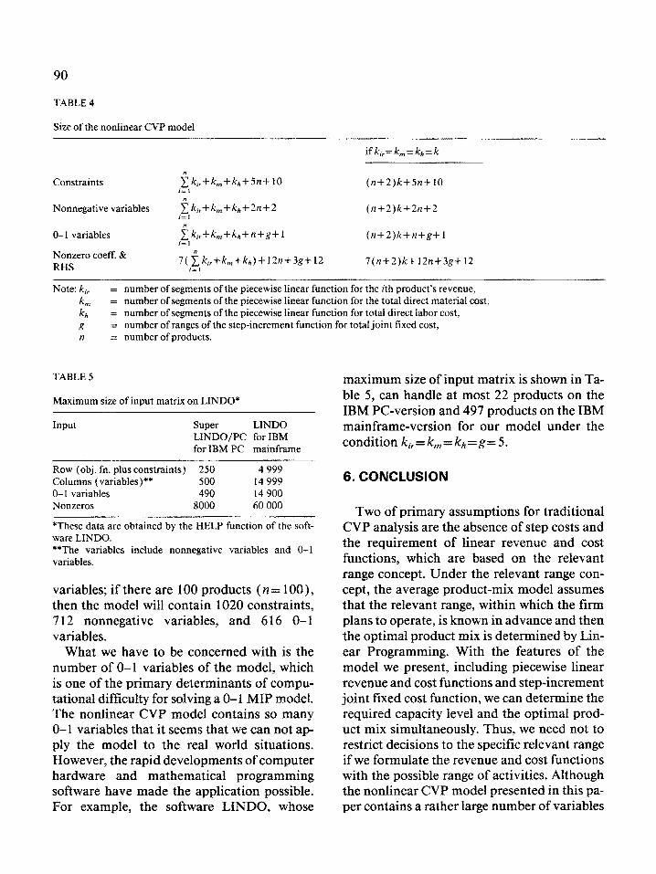
In order to approximate the nonlinear reve- nue and cost functions by the piecewise linear functions, the nonlinear CVP model involves a rather larger number of variables and con- straints as shown in Table 4. For the illustra- tive example in Section 4, y1= 3, k,,= kzr= k3r = 2, km= 3, kh= 2, and g= 2; therefore, there are 36 constraints, 19 nonnegative variables, and 17 0- 1 variables.

Accordingly, the nonlinear CVP model will become larger, when used to describe the real world problems. Suppose that all the nonlinear revenue and cost functions can be approxi- mated by a 5-segment piecewise linear func- tion (i.e., k,=k,=kh=5) and that g=5. Un- der this condition, if there are 10 products ( n = 10 ) , then the model will contain 120 con- straints, 82 nonnegative variables, and 76 O-l

90

TABLE 4

Size of the nonlinear CVP model

ifk,,=k,=k,=k

Constraints (n+2)k+Sn+ 10

Nonnegative variables i k,,+km+kh+2n+2 r=l

(n+2)k+2n+Z

O-1 variables ik,,+k,,,+k,,+n+g+i ,=I

(n+2)k+n+g+ 1

Nonzero coeff. & RHS

7(iki,+k,+kh)+12n+3g+12 iPl

7(n+2)k+ 12n+3g+ 12

Note: k,, = number of segments of the piecewise linear function for the ith product’s revenue,

k, = number of segments of the piecewise linear function for the total direct material cost,

k+, = number of segments of the piecewise linear function for total direct labor cost,

g = number of ranges of the step-increment function for total joint fixed cost, n = number of products.

TABLE 5

Maximum size of input matrix on LINDO*

Input Super LINDO LINDO/PC for IBM for IBM PC mainframe

Row (obj. fn. plus constraints) 250 4 999 Columns (variables)** 500 14 999 0- 1 variables 490 14 900 Nonzeros 8000 60 000

*These data are obtained by the HELP function of the soft- ware LINDO. **The variables include nonnegative variables and O-1 variables.

variables; if there are 100 products (y1= loo), then the model will contain 1020 constraints, 712 nonnegative variables, and 616 O-l variables.

What we have to be concerned with is the number of O-I variables of the model, which is one of the primary determinants of compu- tational difficulty for solving a O-l MIP model. The nonlinear CVP model contains so many 0- 1 variables that it seems that we can not ap- ply the model to the real world situations. However, the rapid developments of computer hardware and mathematical programming software have made the application possible. For example, the software LINDO, whose

maximum size of input matrix is shown in Ta- ble 5, can handle at most 22 products on the IBM PC-version and 497 products on the IBM mainframe-version for our model under the condition ki,= k, = kh =g= 5.

6. CONCLUSION

Two of primary assumptions for traditional CVP analysis are the absence of step costs and the requirement of linear revenue and cost functions, which are based on the relevant range concept. Under the relevant range con- cept, the average product-mix model assumes that the relevant range, within which the firm plans to operate, is known in advance and then the optimal product mix is determined by Lin- ear Programming. With the features of the model we present, including piecewise linear revenue and cost functions and step-increment joint fixed cost function, we can determine the required capacity level and the optimal prod- uct mix simultaneously. Thus, we need not to restrict decisions to the specific relevant range if we formulate the revenue and cost functions with the possible range of activities. Although the nonlinear CVP model presented in this pa- per contains a rather large number of variables

and constraints, the rapid developments of computer hardware and mathematical pro- gramming software have overcome this. In conclusion, it seems possible that the nonlin- ear CVP analysis will be adopted as exten- sively as the traditional CVP analysis was.

ACKNOWLEDGEMENT

This research was supported by the National Science Council of the Republic of China un- der grant NCS78-0415-EOl l-03.

REFERENCES

Jaedicke, R.K., 196 1. Improving breakeven analysis by linear programming techniques. NAA Bulletin, March: 5-12. Killough, L.N. and Leininger, W.E., 1984. Cost Ac- counting: Concepts and Techniques for Management. West Publishing Company, St. Paul, MN, pp. 398-405. Charnes, A., Cooper, W.W. and Ijiri, Y., 1963. Break- even budgeting and programming to goals. J. Account- ing Res., 1 ( 1): 16-43. Hartley, R.V., I97 1. Decision making when joint prod- ucts are involved. The Accounting Rev., XLVI (October): 746-755. Sheshai, K.M. El., Harwood, G.B. and Hermanson, R.H., 1977. Cost volume profit analysis with integer goal pro- gramming. Manage. Accounting, 54(4): 43-47. Beale, E.M.L. and Tomlin, J.A., 1970. Special facilities in a general mathematical programming system for non- convex problems using ordered sets of variables. In: Lawrence, J., (Ed.), Proc. 5th Int. Conf. Oper. Res., Tavistock, London, 447-454.

7

8

9

10

I1

12

13

14

15

16

17

91

Williams, H.P., 1985. Model Building in Mathematical Programming, 2nd edn. John Wiley & Sons Ltd., New York, pp. 173-l 77. Driebeek, N.J., 1966. An algorithm for the solution of mixed integer programming problems. Manage. Sci., 12(7): 576-587. Benders, J.F., 1962. Partitioning procedures for solving mixed-variables programming problems. Numer. Math., 4: 239-252. Lemke, C.E. and Spielberg, K., 1967. Direct search zero- one and mixed integer programming. Oper. Res., 15: 892-914. Davis, R.E., Kendrick, D.A. and Weitzman, M., 1971. A branch-and-bound algorithm for O-l mixed integer programming problems. Oper. Res., 19: 1036-1044. Beale, E.M.L. and Forrest, J.J.H., 1976. Global optimi- zation using special ordered sets. Math. Programming, 10: 52-69. Martin, R.K. and Schrage, L., 1985. Subset coefficient reduction cuts for 0- 1 mixed-integer programming. Oper. Res., 33(3): 505-526. Johnston, E.L. and Powell, S., 1978. Integer program- ming codes. In: Greenberg, H., ( Ed. ) , Design and Imple- mentation of Optimization Software. Sijthoff & Noor- dhoff, Alphen aan den Rijn. Land, A.H. and Powell, S., 198 1. A survey of available computer codes to solve integer linear programming problems. QSSMS Discussion Paper No. 59, Univ. Kent, Canterbury (April). Schrage, L., 1986. Linear, Integer and Quadratic Pro- gramming with LINDO, 3rd edn. The Scientific Press, Redwood City, CA. Schrage, L., 1987. Linear, Integer, and Quadratic Pro- gramming with LINDO-User’s Manual, 3rd edn. The Scientific Press, Redwood City, CA.

(Received January 3 I, 1989; accepted December 2 I, 1989)