Nonlinearities in Exchange-Rate Dynamics:

Chaos?

Vitaliy Vandrovych*

First draft: June11, 2005

This draft: March 17, 2007**

Abstract*** Deterministic chaotic systems represent an appealing new way to model an economy, especially financial markets. They allow the generation of interesting dynamics without exogenous shocks and are unpredictable in the long run. In this paper, I test the hypothesis of chaotic dynamics in exchange rates by applying tools from dynamical systems theory. I find that exchange rate returns are highly nonlinear even when a GARCH-type process is fitted to the data and this result is compatible with chaos. But the calculation of two other prerequisites of chaotic dynamics, namely the correlation dimension and the maximum Lyapunov exponent, rejects the hypothesis of chaos in the data. I emphasize the importance of the proper implementation of chaos tests, as in limited data sets there is a tendency for downward bias in estimates of correlation dimension and this might lead to an incorrect conclusion that chaos is present in the data. As pure chaotic dynamics is not observed in the data, I stress the significance of considering a dynamic noise element in theoretical chaotic asset pricing models.

Keywords: Exchange rate dynamics, chaos, correlation dimension, Lyapunov exponents, BDS test

JEL classification: C22, C49, C51, C63, F31, G12

______________________________________________________________ * Ph.D. candidate, International Business School, Brandeis University, vivandr@brandeis.edu

** Early draft of the paper was titled: “Study of Nonlinearities in the Dynamics of Exchange Rates: Is There

Any Evidence of Chaos?” In this edition of the paper I use longer data set for 4 instead of 6 exchange rates.

*** I would like to thank Blake LeBaron, Carol Osler, and the participants of the 11th International

Conference on Computing in Economics and Finance, and the 14th annual symposium of Society for

Nonlinear Dynamics and Econometrics for providing valuable comments and suggestions on the initial

drafts of the paper. All remaining mistakes are mine.

2

1. Introduction

Traditional structural models of exchange rate determination tend to perform

poorly when confronted with data, both in in-sample and out-of-sample forecasting1.

During the last two decades a number of nonstandard models of asset price determination

were developed that attempt to accommodate the diversity of the economic agents and

their limited access to information and capabilities of processing it when making

economic decisions 2. Simple models with heterogeneous agents frequently are successful

in replicating many stylized facts observed in financial data, such as a large trading

volume, volatility persistence, sudden swings in the market behavior or fat tails of return

distributions (LeBaron, 2006).

In the majority of cases these models are highly nonlinear and result in a wide

range of dynamic behavior, including chaotic dynamics, such as in De Grauwe et al

(1993), Lux (1998), Brock and Hommes (1998), Da Silva (2001), Federici and Gandolfo

(2002), De Grouwe and Grimaldi (2006) among others. The intellectual appeal of such

models is that in many cases they do not require exogenous shocks to exhibit interesting,

real- life like dynamics as it is generated endogenously through the interaction of agents,

and evolutionary change of their strategies.

The possibility of chaotic dynamics in asset prices has a number of implications.

As chaos is by definition a deterministic phenomenon, it implies that observed financial

time series which exhibit highly nonlinear and erratic behavior are in fact a product of the

deterministic system. One of the features of chaotic signals is that even if the dynamical

system generating data is known, and starting points are available, only very short term

forecasting is possible due to the sensitive dependence on the initial conditions (SDIC

thereafter), - the hallmark of chaos. Very small mistakes in the measurement of initial

conditions (and they are unavoidable in economics data) would result in completely

useless predictions of the future states of the system. This certainly would invalidate any

long term forecasting as such. At the same time, as a chaotic trajectory always stays on the

1 Refer to Sarno and Taylor (2002: chapter 4) for detailed analysis of exchange rate determination theories and their empirical performance. 2 See Cars Hommes (2006) for the excellent survey of this fast growing literature.

3

attractor3 in the long run, it is possible to make predictions about the limits in which the

economic system will evolve over time.

In this paper we single out one feature of the above mentioned literature, namely

the possibility of chaotic dynamics, and test it empirically using the exchange rate data.

Tools from dynamical systems theory, such as correlation dimension and maximum

Lyapunov exponents are used to make distinction between data produced by random and

deterministic systems 4. Our analysis indicates that although exchange rate returns are not

independently and identically distributed (iid thereafter) and contain some important

nonlinear dependence, they do not possess the features that are required to classify them

as chaotic.

As the testing procedures involve a number of subjective decisions on the selection

of parameters and interpretation of the graphical information, we elaborate also on the

importance of the proper implementation of chaos testing techniques. In particular, we

show that the omission of Theiler correction5 to the Grassberger and Procaccia algorithm

may lead to an incorrect conclusion of chaotic dynamics in some variables.

Our results do not invalidate the theoretical literature that implies a chaotic origin

of financial time series. Rather it indicates that some amount of stochastic ingredients

(dynamic noise) has to be present in a model that attempts to replicate the observed

financial data. While internal interactions of heterogeneous agents are important, and may

serve as the skeleton of the model, exogenous “news” has to be taken into account as well,

not necessarily as a driving force but as “noise”, albeit small, that has important

implications for the evolution of the economy.

The rest of the paper proceeds as following. In section 2 we provide short

background information on the notion of chaos and methods used to test it in empirical

data. Section 3 outlines the results of the previous studies on chaos in exchange rate series.

Section 4 describes the data used in the paper. Section 5 gives details on testing

methodology and results that we obtained. And section 6 concludes.

3 Bounded although topologically strange set. 4 See Brock (1986) for a rigorous mathematical introduction to the tests that help to distinguish between random and deterministic systems. 5 This correction is considered as a norm in the physics empirical studies but is not widely used in economics papers.

4

2. Detecting chaos in empirical data: methodology

There is no unique definition of chaos, and the most common way to introduce it is

by listing the important features tha t have to be present in any chaotic system. The signal

is chaotic if it has all of the following attributes: it is nonlinear, has SDIC, a strange

attractor, continuous broadband Fourier power spectrum, at least one positive Liapunov

exponent and ergodicity6. Although any chaotic signal is produced by some purely

deterministic system7, visually it is indistinguishable from the stochastic one.

In this paper we study three of the above characteristics, namely: nonlinearity, by

applying BDS test, the strange attractor, by calculating correlation dimension, and SDIC,

by estimating the maximum Lyapunov exponent. The remaining part of this section

elaborates on how to calculate these quantities using the empirical data.

2.1 General background and phase space reconstruction

Let’s assume that the dynamics of an economy is generated by some unknown

deterministic dynamical system. The set of all possible states of a system is called a phase

space. Let’s consider a finite-dimensional state space nR , in which state of the system is

characterized by a vector nR∈s . The dynamics of such a system may be represented

either by n-dimensional map:

)(1 tt F ss =+ (1)

or by a system of n first-order ordinary differential equations:

(t))((t)dtd sfs = (2)

Given some initial conditions, the solution of the system (also called the orbit or

trajectory) will be attracted to some subspace of the phase space, which is called attractor

of the system, after a sufficiently long transition period. Typically, for dissipative systems8

6 See De Grauwe et all (1993, pp.34-35), Abarbanel (1995) or Kantz and Schreiber (2004) for a detailed introduction to the subject. 7 Mathematically given by some system of nonlinear difference or differential equations. 8 Dissipative systems are systems for which volume in the phase space is usually contracted under the time evolution.

5

the volume that is filled by an attractor is much smaller than the volume of the phase

space.

For some systems, motion within an attractor is unstable. It is expressed in an

exponential separation of orbits of points that are close to each other on the attractor

(Eckmann and Ruelle (1985))9. Attractors with such an instability property are called

strange attractors, and correspondingly systems that possess them are called chaotic.

In empirical studies, the states of a dynamical system, ts , are not observed, and the

deterministic equation of motion, )(1 tt F ss =+ , is not known. What is available to the

researcher, is just some scalar time series of measurements, say N daily exchange rates Nttx 1}{ = , which are related to ts through the observer function, )( tshx t = , also not

known. The situation can be even more complicated when some random measurement

error10 is also present:

tt hx εγ *)( += ts , )1,0(IIDt ≈ε , (3)

where RRh n →: is an observer function that maps the state of the original system to

the scalar time series, γ is noise level, and tε stands for measurement error11.

Knowledge of the precise initial conditions for the variables of the original system

and knowledge of the functions F and h that represent the dynamics of the system would

enable us to predict the exact state of the system at each point in time.

The embedding theorem of Takens (1981) provides the conditions under which the

properties of original chaotic system may be reconstructed from the scalar time series of

observations. The process of rebuilding the state vectors from the observed data is called a

phase space reconstruction. This method involves creation of m-dimensional ‘histories’,

),...,,( )1( ττ −++= mtttt xxxX , where m is the embedding dimension12, and τ is the time

delay13. Takens proved that the resulting reconstructed trajectory, )',...,,( 21 MXXXX = ,

9 As an attractor normally is bounded, this special separation is evident only for short time periods until the boundary of the attractor is reached. 10 This is also called observational noise. 11 Here we follow the notations used in Bask M. (2002). 12 A theoretically sufficient condition for m to be the embedding dimension is m>2d, where d is the actual topological dimension of the attractor, but in practice it is frequently the case that much lower m will work. 13 One of the frequently used methods for the time delay is to set it equal to the first zero-crossing of the autocorrelation function. Another method uses the delay that corresponds to the first local minimum of the mutual information function (see Diks C. 1999, p.23).

6

with M = N – (m-1) τ , has topological properties that are identical to the properties of the

original system. Hence, it is possible to learn the dynamic characteristics of the unknown

system by studying the dynamics of the reconstructed orbit.

Therefore, any study of chaotic dynamics in empirical data starts with the phase

space reconstruction, followed then by application of tests that calculate the invariants of

motion, such as fractal dimensions and maximum Lyapunov exponent. Finite (and low)

fractal dimension is a necessary but not a sufficient condition for chaos. When it is

combined with a positive maximum Lyapunov exponent, it represents a strong indication

of chaotic origin of the data.

2.2 BDS test

As chaos is a nonlinear phenomenon, it is suggestive to find if any nonlinear

dependence is present in the data before proceeding to more direct chaos tests. This task

may be accomplished by the BDS test of Brock et al14 (1987), which evaluates the null

hypothesis that data is iid. Its rejection implies some kind of dependence that may come

from a number of different models, stochastic and deterministic, linear and nonlinear.

BDS statistics has an asymptotically standard normal distribution, and any dependence in

the data will result in the test statistic being larger than the critical value for the standard

normal distribution. In order to eliminate possible linear dependence, the time series is

frequently pre-filtered by an autoregressive model, and the BDS test is applied to the

residuals. If the null hypothesis is rejected even in this case, the presence of nonlinear

dependence is established in the data.

Two major invariant quantities are used for the classification of chaotic systems:

correlation dimension and the maximum Lyapunov exponent 15. These invariants do not

depend on the initial conditions or coordinate system in which the dynamics is studied,

and are preserved under smooth nonlinear changes of coordinate system.

14 See also Brock et al (1996) for the published version of the paper. 15 See Abarbanel (1996), chapter 5, for detailed description.

7

2.3 Correlation dimension

As mentioned above, chaotic dynamical systems possess strange attractors. One of

the features of strange attractors is that they have a fractal dimension which is smaller than

the number of degrees of freedom of the system (Grassberger and Procaccia 1983a) (GP

thereafter). Hausdorff dimension and information entropy used to be the most commonly

applied measures of the attractor’s structure. Papers by GP (1983a, 1983b) introduce a

new measure which was named correlation dimension, which has since been

predominantly used in empirical studies. In contrast to the old measures, correlation

dimension is sensitive to the process of coverage of the attractor (how frequently different

parts of the attractor are visited by the trajectory), and moreover it is computationally

simpler and allows characterization of the attractor even for high-dimensional dynamical

systems (GP 1983a).

Correlation dimension is based on the notion of correlation integral that measures

spatial correlation of points on the attractor. An important contribution of GP is that they

used result of Takens (1981), and showed how to calculate the correlation dimension

given only the scalar time series. This procedure is described below.

Given the scalar time series, Nttx 1}{ = , m-dimensional histories,

),...,,( )1( ττ −++= mtttt xxxX , are created. Then this reconstructed orbit,

)',...,,( 21 MXXXX = , with M = N – (m-1)τ , may be used for calculation of the

correlation integral, C(M,m,r), that is given by the following formula:16

∑ ∑−

= +=−−

−=

1

1 1||)||(

)1(2

),,(M

i

M

ijji XXr

MMrmMC θ , (4)

where r is the radius, m is the embedding dimension, Xi and Xj are m-dimensional

histories, and )(sθ is Heavyside function that is given by 1)( =sθ if 0≥s , and 0)( =sθ if

0<s . The correlation integral provides the fraction of pairs (Xi, Xj) having distance

between them smaller than a chosen radius r, and may be interpreted as the probability of

the distance between any two m-histories being smaller than r. GP show that cDrrC ∝)( ,

and define the correlation dimension as:

16 See for example, Diks (1999, p.19).

8

rrmMC

DrM

mc log

),,(loglimlim

0→∞→= . (5)

The correlation dimension may be considered as an effective number of degrees of

freedom or “a lower bound on the number of independent variables which would be

required to model the series” (Brooks, 1998, p.272).

When analyzing empirical data, the number of m-histories that can be created, M,

is finite, and correspondingly the radius r cannot be too small. In order to distinguish

between deterministic chaos and random noise, one embeds data in higher and higher

spaces (by increasing the embedding dimension m) and calculates the slope of log

C(M,m,r) against log(r) for each m. For random noise this slope will increase indefinitely

with the increase in m (slope will be approximately equal to m). For a signal that comes

from a deterministic system the slope will reach the value of correlation dimension and

then will become independent of further increases in m.

Very important modification to GP method was proposed by Theiler (1986)17. He

showed that in the limited data sets correlation dimension estimates calculated directly

from the GP formula would be biased downward due to the “temporal” correlation in the

data. Temporal correlation, as opposed to geometrical correlation (that the correlation

integral is supposed to measure), is the outcome of the fact that points on the

reconstructed orbit that are close in time, are also close in the phase space. If those points

are not excluded when calculating the correlation integral, estimates would be understated

and it is possible to obtain low estimates even for stochastic systems. In order to overcome

this problem, the GP formula has to be modified as follows:

∑ ∑−

= +=−−

−−−=

WM

i

M

Wijji XXr

WMWMrmMC

1||)||(

)1)((2

),,( θ , (6)

where 1≥W is the Theiler correction (Diks, 1999, p.20) which is recommended to be

chosen at least as high as the autocorrelation time. We believe that this correction is not

frequently used in economic empirical studies and this might be the reason for a number

of small estimates reported that are just artifacts of the dynamical correlation in the data.

GP (1983b) also notes that if there is some random noise that is imposed on an

otherwise deterministic chaotic signal, then a plot of log C(M,m,r) on log(r) will have two

17 See Kantz and Scheiber (2002, p.80) for the discussion.

9

regions. In the region with the small r, in which random noise will dominate chaotic

signal, the slope of the line will be approximately equal to the embedding dimension. In

the region with the higher r, the slope of the log C(M,m,r) against log(r) will converge to

the correlation dimension of the deterministic attractor. Eckmann and Ruelle (1985) call

such plots “curves with knees”, and their presence may indicate that an underlying chaotic

signal is contaminated with noise.

One of the limitations in the use of this indirect classification test for chaos is that

the number of data points in empirical applications is usually very small while the precise

calculation requires an almost infinite amount of data. Eckmann and Ruelle (1992)

provide the formula that allows calculating an approximate maximal possible estimate of

the correlation dimension:

)/1log(log2

max ρN

d = (7)

where maxd is the maximal possible estimate of correlation dimension for a given data set;

N is the number of data points in the scalar time series;

and Dr=ρ is relative magnitude of r used in the GP algorithm in relation to the

diameter of the reconstructed attractor. As the GP algorithms calls for r that approaches

zero, Eckmann and Ruelle (1992) argue that it is necessary to look at 1.0≤ρ . The paper

concludes that a reliable estimate of dimension has to be substantially below maxd , and it

can be calculated only when the linearity of GP plots at small log r can be verified, and

there is convergence of slopes for different embedding dimensions.

Another limitation in the use of correlation dimension as the chaos classifying tool

is the absence of a theory that would provide its distributional characteristics18. Therefore,

in this paper, we are interested not as much in the exact estimates of the dimension for

different quantities, but in the qualitative picture of the convergence or divergence of

those estimates, and also in the similarities or differences in the estimates for different

currency pairs.

18 See, for examp le, Barnett et al. (1995).

10

2.4 Maximum Lyapunov exponent

A distinguishing feature of chaotic dynamical systems is SDIC. SDIC makes

deterministic chaotic systems completely unpredictable in the long run because the

distance between two orbits that start from very close initial points grows exponentially.

Lyapunov characteristic exponents quantitatively measure the stability or instability of the

dynamical system. A necessary condition for the presence of chaotic dynamics in a time

series is a positive maximal Liapunov exponent.

One of the first methods developed to estimate the maximum Lyapunov exponent

from data was by Wolf et al (1985). However, it requires a large amount of data and is

sensitive to noise. In this paper we are using the Rosenstein et al (1993) method which is

simple compared to other methods19, and is tested to work well in small samples and with

data contaminated with noise.

This approach relies on the method of delays for the phase space reconstruction,

similar to the GP algorithm for correlation dimension. After the dynamics of the system is

reconstructed and orbit )',...,,( 21 MXXXX = obtained, the next step is to locate the

nearest neighbor for each point, and calculate the initial distance between nearest

neighbors:

pijXj XXdi

||||min)0( −= , (8)

where ||...||p denotes the norm in m-dimensional reconstructed space20. The search for the

nearest neighbor is constrained by the requirement that nearest neighbors should have a

temporal separation larger than the mean period of the time series, which can be

calculated as the reciprocal of the mean frequency of the power spectrum. This

requirement allows interpreting the nearest neighbors as two close points from different

trajectories. The largest Lyapunov exponent may be estimated as the mean rate of

separation of nearest neighbors.

Rosenstein et al (1993) method then proceeds as follows. As a maximum

Lyapunov exponent measures the speed of exponential divergence or convergence, the

19 It was used by Bask (2002) and Brzozowska and Orlowski (2004) in the context of exchange rate time series. 20 The Euclidean norm is proposed in the original paper but any other norm will work. We will use the “maximum” norm in our estimation.

11

following formula may be used to show the relation connecting initial distance between

nearest neighbors and distance after some time, t:

)*exp(*)0()( 1 tdtd jj λ≈ , (9)

where t is the number of separation steps, 1λ is the largest Lyapunov exponent, and )(td j

is the distance between nearest neighbors after t separation steps.

By taking the logs of both sides of the above formula we obtain:

tdtd jj *)0(log)(log 1λ+≈ (10)

Then averaging over all the pairs of nearest neighbors (over all j), we get

tdtd jj *)0(log)(log 1λ+≈ (11)

where ... denotes the average over all values of j. Then the largest Lyapunov exponent,

1λ , is estimated by regressing the average log distance after t separation steps on the

number of separation steps.

Rosenstein et al. (1993) shows that this method works satisfactorily even for very

small data sets, is not very sensitive to time delay, and provides good estimates even when

some small amount of observational noise is present (1-10%). What is more important, it

allows discriminating between chaotic and stochastic systems. In stochastic systems

nearest neighbors will neither diverge nor converge, and a flat plot of )(log td j versus t

is expected.

3. Previous empirical studies of chaos in exchange rates

The interest in the possibility of chaotic dynamics in economic time series

emerged in the 1980s, and it was stimulated by the theoretical possibility of explaining

seemingly random fluctuations and large movements in financial markets by means of

deterministic systems 21 (Hsieh, 1991). Major methodologies and testing procedures were

established at that time, mostly by adjusting the tools used in physics and other natural

sciences. A summary of the results of the initial empirical studies is reported in LeBaron

(1994). The main conclusion of the early literature is that empirical evidence for chaotic 21 This implies that chaotic models are able to generate nonlinear dynamics endogenously while the traditional models rely on the external shocks to have interesting dynamics.

12

dynamics in economic time series is very fragile, although most studies found some

support for the presence of nonlinear structures in the examined series. Hsieh (1991)

stresses that only low dimension chaotic behavior is of interest to economists, as high

dimensional chaotic processes are difficult to detect with limited amount of data.

Studies dedicated to the search for chaos in asset prices, and in exchange rates in

particular, may be subdivided into positive, cautiously positive and negative by their

results concerning chaos in the data. The methodological tools also differ from paper to

paper.

One of the early indirect studies of chaos in exchange rates is by Hsieh (1989).

Hsieh researches whether exchange rate returns on five major currencies contain any

nonlinearities. As the presence of nonlinearity is the important prerequisite for chaos, such

study is the necessary first step. The paper applies the BDS test, which strongly rejects the

iid hypothesis in all currency pairs, even when linear dependence is filtered out by an

autoregressive process. Trying to discriminate between stochastic and deterministic

nonlinear dependence, Hsieh fits the AR-GARCH (1, 1) model to the returns and then

applies the BDS test to the standardized residuals. While stochastic origin is confirmed for

Canadian Dollar, Japanese Yen and Swiss Franc returns, strong unexplained nonlinearity

is still present in British Pound returns and in returns of the Deutsche Mark, leaving

question of the origin of nonlinearity in those currencies open.

Among the early cautiously positive studies of empirical chaos is the paper by

Scheinkman and Lebaron (1989), which considers daily and weekly returns on the value-

weighted stock portfolio. They report correlation dimension equal to 5.7 for weekly

returns, which does not imply low-dimensionality of the studied series but suggests some

kind of nonlinear structure in the data. This result is strongly reinforced by the experiment

with the “scrambled” series that are obtained by regressing original return data on their

past values, estimating residuals, and then adding the randomly selected residuals to the

estimated linear system. Estimates of correlation dimension for scrambled data turned out

to be much higher than for the original series.

De Grauwe et al. (1993) provide mixed evidence on chaos in exchange rates. They

consider the period from 1973 to 1990 and their sub-periods and calculate the dimension

for DM/USD, BP/USD and JPY/USD returns. Absence of chaos is reported for DM/USD,

13

but rather strong indication of chaos, with the estimates of correlation dimension around 2,

are obtained for BP/USD and JPY/USD for 1973-1982 and the overall period.

A number of chaos positive papers appear in the literature. The study by Bajo-

Rubio et al. (1992) applies the correlation dimension and the Lyapunov exponents to

detect the presence of chaos in Spanish Peseta – U.S. dollar spot and forward rates, using

daily data for 1985-1991. Due to the presence of unit root in the level series, tests are

applied to first differences of the original data. The correlation dimension found ranges

from 2.7 to 3.2 for spot rates, and 1.8 to 3.3 for forward rates, suggesting the presence of

low dimensional chaotic dynamics. Lyapunov exponents, calculated using the Wolf

algorithm, are all positive, further supporting the presence of chaos.

Bask M. (2002) studies the chaos in daily Swedish Krona exchange rates against a

few major currencies using the Rosenstein et al (1993) method to calculate the maximum

Lyapunov exponent and the blockwise bootstrap procedure of Bask and Gencay (1998) to

find the critical values of the estimates. His estimates are positive in many sub-periods,

compatible with the presence of chaos. The same methodology is applied by Brzozowska-

Rup and Orlowski (2004) to daily average US Dollar against Polish Zloty exchange rates

for the period 1993-2003, and also for some embedding dimensions estimates of the

maximum Liapunov exponent are positive, which is consistent with chaos.

A few papers report a definite rejection of chaos in exchange rates. The paper by

Brooks (1998) studies ten daily sterling-denominated exchange rate returns. A few of the

series exhibit some weak saturation of the correlation dimension estimates at around 4.5-6

level when the embedding dimension is increased to 15. Then the Wolf et al. (1985)

algorithm and the Dechert and Gencay (1990) neural network technique are applied to

determine the Lyapunov exponents. Estimates produced by the Wolf algorithm are

positive in all cases, but this is invalidated by similar positive estimates obtained for

surrogate data. Estimates obtained from the second method are consistently negative and

the overall conclusion reached is strictly chaos negative.

Guillaume (1995, 2000) uses intraday exchange rates to study the possibility of

chaos in exchange rate returns and their absolute values using the GP (1983) algorithm.

The author looks at different sampling frequencies, namely 15, 30, and 60 minutes, over

the 6-year period starting at the beginning of 1987 and until the end of 1992 for four major

14

currency pairs: USD/DEM, USD/GBP, USD/JPY, and USD/FRF22. A few different

methods of the attractor reconstruction are used. Neither of the methods can produce the

convergence of the correlation dimension estimates suggesting the absence of low

dimensional chaos in the studied series.

Serletis and Shahmoradi (2004) provide convincing evidence of the absence of

chaotic dynamics in CAD/USD returns for the 1974-2002 time period. They calculate the

maximum Lyapunov exponent using the Nychka et al. (1992) method and additionally

construct the confidence intervals for the estimates using the procedure presented in

Shintani and Linton (2004). Estimates obtained for the embedding dimension up to 6 are

all negative, rejecting the low dimensional determinism in this exchange rate.

4. Data description

In order to test for evidence of chaotic dynamics in exchange rates, we consider 4

major currency pairs, namely U.S. $ to 1 British Pound (USD/BP), Japanese Yen to 1 U.S.

$ (JPY/USD), Swiss Franc to 1 U.S. $ (CHF/USD), and Canadian $ to 1 U.S. $

(CAD/USD), given by noon buying rates in New York and reported at the webpage of the

Federal Reserve Bank of St. Louis23. Our data set spans the period from January 1975

until June 2006 and contains 7897 daily observations for each currency pair.

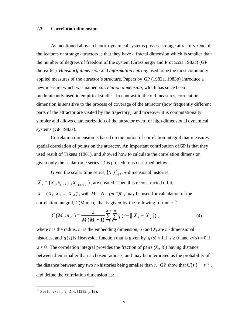
Similarly to many other papers, we study the exchange rate returns, but

additionally we include volatility and normalized exchange rates, definitions of which are

provided below. Let St denote the level of the exchange rate at time t. Exchange rate

return at time t is calculated as the log difference of consecutive exchange rate levels:

)ln()ln( 1−−= ttt SSr

We define daily volatility as the absolute value of exchange rate returns :

Vt = |rt|.

22 A small number of data points is a typical drawback of the empirical studies of chaos in economics, and the use of intraday data seemingly overcomes this problem. But, as is mentioned by Hsieh (1991), high frequency data are contaminated by artificial dependencies caused by the market microstructure effects of fore x trading. At the same time when long time series over many years are used, then there is problem of nonstationarity. 23 http://research.stlouisfed.org/fred2/categories/94

15

Normalized exchange rate is created as current exchange rate divided by a 50-day simple

moving average:

∑=

−=49

0

/i

ittt SSX ,

and it may be regarded as a technical trading signal24. As similar technical signals are

heavily used in the forecasting by technical traders we are curious to see if any

deterministic dynamics can be found in such variable.

Figures 1-4 present a graphical description of the above mentioned series; and

tables 1 (i- iv) show summary statistics. The same series, with the addition of DEM/USD

were studied in Hsieh (1989), for the shorter period of 1974-1983. We would like to note

that the returns in our sample have smaller kurtosis than in Hsieh’s sample, implying

closer approximation by the normal distribution, although fat tails are still characteristic

for these series. While the mean level of the returns is close to zero, there are instances

when daily changes in exchange rates are high, like -5.65% for JPY/USD or 5.8% for

CHF/USD. The least volatile exchange rate in our sample is CAD/USD, with lowest

volatility and smallest range of returns. The highest volatility is observed in the CHF/USD

currency pair.

An important requirement for the time series analysis is the stationarity of the

data. Augmented Dickey-Fuller and Phillips-Perron unit root tests are applied to check for

the stochastic trend in the exchange rate levels. All specifications suggest a presence of

the unit root in the level series25. Therefore in what follows we will study first differences

of exchange rates (exchange rate returns) that are stationary according to the above

mentioned tests. Normalized exchange rates and volatilities also pass the tests for

stationarity.

Figure 5 provides the description of the serial correlation in our data. Exchange

rate levels are highly persistent, with first zero of autocorrelation function ranging from

781 lags for USD/BP to 2574 lags for CHF/USD. Log-differencing removes almost all

autocorrelation, and as a result exchange rate returns are practically uncorrelated26. At the

24 I thank Blake LeBaron for suggesting me to consider this variable. 25 Except the JPY/USD exchange rate, for which the null hypothesis of unit root cannot be rejected at the 1% significance level, but is rejected at the 5% significance level. 26 Autocorrelation is considered significant with 95% confidence if it lies outside the interval [-2n-1/2, 2n-1/2], where n is the number of data points used in calculation.

16

same time, absolute values of returns (volatility variables) exhibit strong linear

dependence which differs substantially among currencies27. Normalized exchange rates

are much less persistent than exchange rate levels, and their autocorrelation declines to

zero after approximately 40-100 lags, but if the number of legs is increased further,

prolonged periods of nonzero autocorrelations are present, reflecting the dependence

structure that is imposed on this variable by including the 50-day moving average.

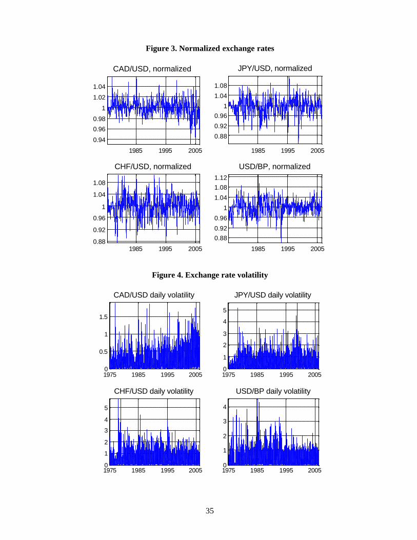
For the low-dimensional chaotic systems it is possible to provide a qualitative

information about the dynamics of the system by means of a phase portrait. It is

constructed as a plot of two or more dynamical variables against each other. For

experimental data a phase portrait is constructed by plotting the variable of interest against

the same variable but delayed in time. The time delay can be chosen similarly to the phase

space reconstruction as the first zero of ACF, first minimum of AMI or using some other

method.

Figure 6 provides phase portraits for all variables in two-dimensional space28.

Time delays are chosen to be equal to the first zero of the ACF29. Plots for exchange rate

levels look quite interesting and suggest that there is some nonlinear dependence structure

present there, implying the possibility of chaotic dynamics. But non-stationarity and very

large delays required for the elimination of the autocorrelation prevents us from applying

chaos tests directly to exchange rate levels. Plots for returns illuminate a quite different

picture: points on the reconstructed trajectory are distributed much more evenly in the

phase space, with the concentration in the region close to zero. Even if there is some

structure in these series it would require a much higher-dimensional space to see it. Phase

portraits for normalized exchange rates are visually similar to the plots for returns series,

but they exhibit more structure at the same time. And graphs for volatilities, that are the

projections of returns’ plots onto the first quadrant, do not suggest the presence of a low

dimensional strange attractor.

27 The first zero of ACF for CAD/USD volatility is observed after 1631 lags, for JPY/USD volatility – after 445 lags, for CHF/USD volatility – after 90 lags, and finally for USD/BP volatility – after 324 lags. 28 Certainly if the dimension of the attractor is much higher than 2 then phase portrait in two dimensional space will be not very informative. 29 For exchange rate levels they are as following: CAD/USD – 1588, JPY/USD - 2555, CHF/USD - 2573, and USD/BP – 780. As returns are practically uncorrelated we choose time delay 1 for them. Delays for normalized exchange rates: CAD/USD – 43, JPY/USD – 88, CHF/USD – 73, and USD/BP – 105. And finally delays for volatilities are as follows: CAD/USD – 1663, JPY/USD – 444, CHF/USD – 197, and USD/BP – 323.

17

Before proceeding to the calculation of invariants of motion we first apply the

BDS test to the return series in order to establish the presence of nonlinearity in the data.

Following Hsieh (1989), we define distance r in terms of the standard deviation of the

data, ranging from 0.5 to 1.5, while setting the maximum embedding dimension m to 10.

Table 2 (a) reports the BDS statistics for exchange rate returns 30. The null

hypothesis of iid is strongly rejected for all currency pairs. The highest degree of

dependence is observed in CAD/USD returns for which the BDS statistics is consistently

higher in all cases, which is then followed by USD/BP, JPY/USD and finally CHF/USD

returns. Rejection of the null hypothesis in our sample is slightly stronger than in Brock et

al (1991)31, where the same exchange rates but for a much shorter period (1974-1983) are

considered.

In order to remove possible linear dependence in the data we filter returns with the

autoregressive model with maximum number of lags set to 10. We use Akaike

Information Criterions (AIC thereafter) for the selection of the best model. Those are

AR(0) for all returns except USD/BP, for which AR(1) was selected. The resulting BDS

statistics for filtered returns are very close to the ones for the raw data. That confirms that

the rejection of iid in return data is due to some nonlinear dependence in the series.

The above analysis suggests that our data is generated by some nonlinear

processes, which can be stochastic or deterministic. A number of nonlinear stochastic

processes are described in the time series literature and it is impossible to test each of

them. Many empirical financial publications suggest that GARCH type models provide an

accurate description of the return data. Therefore, we fit different AR(p)-GARCH(m,n)

models to the returns32 and then apply the BDS test to the standardized residuals of the

models selected by the AIC criteria.

AIC selects the following models : CAD/USD – AR(2)-GARCH(2,2); JPY/USD –

AR(1)-GARCH(3,1); CHF/USD – AR(1)-GARCH(1,1); and USD/BP – AR(9)-

GARCH(3,1). The results of the BDS test on the standardized innovations of these models

are reported in table 2(b). We use the quantiles of the standard normal distribution to

30 For the calculation of BDS statistic we used a Matlab program provided by Blake LeBaron which is available at http://people.brandeis.edu/~blebaron/soft.html. 31 See table 4.3, page 148. 32 Maximum p is set to 10 and maximum m and n are set to 3.

18

establish the significance of the estimates, although as was noted by Hsieh (1989)33

among others, use of the standard normal distribution for GARCH standardized residuals

is rather conservative, and critical values have to be lower in absolute value.

The BDS test finds slight nonlinearity for CAD/USD and CHF/USD at high

embedding dimensions, but very strong nonlinearity for JPY/USD and USD/BP, except

cases when dimension, m, is low (2, 3, 4) and distance, r, is large (1.25 or 1.5). Therefore,

we may conclude that while CAD/USD and CHF/USD are accurately described by the

stochastic AR-GARCH model, the question of the best model for USD/BP and JPY/USD

returns remains open, and those two currency pairs are potential candidates for

representation by some deterministic model. We will continue this investigation in the

next section by applying correlation dimension and maximum Liapunov exponent criteria

to these series.

5. Empirical results

5.1 Correlation dimension estimation

Correlation dimension is estimated using the GP algorithm outlined in section 2.3.

In all cases we calculate the correlation integral using the “maximum” norm34 that

measures the distance between two vectors as the maximum of the differences between

corresponding coordinates of those vectors. Embedding dimens ion is set in the range from

2 to 12. Time delay,τ , is chosen according to the formula:

)1()/11()( ACFeACF −≤τ , where ACF is the autocorrelation function35. Given that

we have 7896 data points for exchange rate returns, the rough36 estimate of maxd for our

data set is 7.8, calculated using the Eckmann and Ruelle formula reported in section 2.3.

33 See Hsieh (1989), page 363, especially note 4 on that page. See also Brock et al (1991), Appendix F, that provides distribution and quantiles of the BDS statistic GARCH (1,1) standardized residuals for different number of observations and different distance parameter. 34 Use of the Euclidean norm does not change results qualitatively but makes it more difficult to establish scaling regions. 35 This method of choosing time delay was reported to provide the best performance of Rosenstein et al (1993) algorithm for maximum Lyapunov estimation that we use in this paper. 36 Assuming that the diameter of the attractor at the higher embedding dimensions is approximately equal to the diameter at dimension 1.

19

And finally we consider radius in the range from 0.1 to 2.5 standard deviations of the data

with the step equal to 0.05 standard deviations.

In order to evaluate the accuracy of our Matlab code we first test it on the data

produced by the Henon map, for which the true estimate of correlation dimension is

known and is approximately equal to 1.21-1.2537. The Henon map is given by the

following system of difference equations:

.*3.0

,*4.11

1

21

tt

ttt

xy

xyx

=

−+=

+

+

Using (0,0) as the initial condition, the orbit of the Henon map is characterized by chaotic

dynamics whose strange attractor is shown in figure 7. We generate 8896 data points by

the above system, discard first 1000 points as transients, and then use the last 7896 of the

x-series for the estimation of the dimension in order to see how the algorithm works on a

sample size comparable to ours.

The resulting plot of log correlation dimension against log radius for embedding

dimensions from 2 to 12 is presented in figure 8. A clear scaling region is obvious for

small values of r, on which the slope is linear and similar for different embedding

dimensions (this region corresponds roughly to the range of radius from 2.8% to 7% of the

attractor’s diameter). In the region further to the right of this range (the furthest right value

of the radius is equal to 70% of the attractor) scaling behavior is absent, and it would not

be possible to calculate a correlation dimension in this region. Hence, “small” value of

radius is an important prerequisite for obtaining good estimates. Numerical estimates in

table 3 show that the algorithm provides a very accurate approximation of the correlation

dimension for the actual chaotic data38.

5.1.1 Exchange rate returns

Correlation dimension for exchange rate returns is obtained through the following

steps. First we apply the GP algorithm with Thailer correction, W set to 100, to the raw

37 Grassberger and Procaccia (1983b, p201). 38 We still have to be cautious when applying this algorithm to the actual data, because as was mentioned by Kantz and Schreiber (2004, p.78), although correlation dimension estimation is a good tool to measure self-similarity (that can be inferred from fractal dimension) in known chaotic systems, it is less appropriate when applied to systems, the chaotic origin of which has yet to be established.

20

return series. Then we recalculate the dimension for scrambled returns, following the

procedure suggested by Scheinkman, J. & LeBaron (1989) with small modification39. The

idea behind this procedure is that if our original data has some deterministic structure, the

reshuffling should substantially destroy such dependences, and the system should be more

“random” than the original one. As a result, obtained estimates of correlation dimension

should be higher for the reshuffled data.

Similar steps are then applied to the standardized residuals of AR-GARCH models

fitted to return series. As was shown in section 4 by the BDS test, strong nonlinear

dependence is still present in the residuals of JPY/USD and USD/BP return series, and we

expect to see it in the GP plots.

Results are presented in figures 9 (a-d), and table 4 reports estimates of correlation

dimension for cases where a clear scaling region is present.

Opposite to the Henon map, the same method of choosing the radius for return

series (0.1:0.05:2.5 of standard deviation of the data) results in a relative range between

1% and 24% of the attractor’s diameter40.

The plot for CAD/USD returns (figure 9(a)) indicates a stochastic origin of the

series, as expected. This is visible from the absence of any scaling region in the plot of

local slope of the log correlation integral against log of radius, and an increase in the

estimates of correlation dimension with each subsequent embedding dimension. The plot

for CAD/USD scrambled returns looks very similar, with the only difference being that

for high embedding dimensions and small values of radius there are no sufficient data

points and the plot looks jagged in that region. The same absence of evidence for chaos is

also apparent in the graph for standardized GARCH residuals of CAD/USD.

Results for JPY/USD are noticeably different. First of all, there is a clear scaling

region for the middle range of radius (it is shown by dotted lines in fig.9 (b)), which

corresponds to the region between 2.9% and 7.48% of the diameter of attractor. The slope

shows slow tendency to saturation at around 5.3, but saturation is not complete and a

small increase in correlation dimension is still observed when the embedding dimension

39 Scheinkman and LeBaron (1989) regress the original data on past data and estimate residuals from those models. Then they sample with the replacement from the residuals and use the obtained sample for rebuilding the original data using the estimated linear models and the same initial values. We sample with replacement directly from the return series, and consider it the “scrambled” returns. 40 This is the other way to see that return series have substantial probability of extreme values as compared to the Henon map.

21

goes up. At the same time estimates for scrambled returns are substantially higher,

pointing out that some structure is present in the return series, suggesting the possibility of

chaos. But applying formula (7) for the range of radius that corresponds to the scaling

region, it is revealed that the maximum possible reasonable estimate of dimension in that

range is 5 – 6.9. Therefore, our estimate of 5-6 is too close to the critical region, and we

conclude that such a result is due to the small number of data points rather than finite

dimension of the attractor. This conclusion is reinforced by the graph for AR-GARCH

standardized residuals. When JPY/USD returns are adjusted for AR-GARCH structure,

the saturation of the slope disappears and series behaves as purely random.

The case of CHF/USD returns is definitely of stochastic origin. No saturation of

the slope is observed, and the qualitative picture is similar for pure and scrambled returns,

especially when AR-GARCH structure is removed (see fig.9 (c)).

Fig.9 (d) shows the results for USD/BP returns. Although there is a jump in the

dimension estimate when data is scrambled; there is no definite scaling region for raw

returns to calculate the dimension. But when the AR-GARCH effect is taken into account,

a comparatively good scaling region, ranging from 1.3% to 4.7% of diameter, is observed,

on which we may estimate correlation dimension as approximately 5.9 (table 4). However

formula (7) indicates that the maximum possible dimension in this region is between 4.20

and 5.86. Hence, our conclusion is chaos negative in this case.

In summary, we may conclude that there is heterogeneity in terms of data

generating systems for exchange rate returns. For CAD/USD and CHF/USD returns, a

conclusion of stochastic origin seems unquestionable, and that is what we would expect

given the results of the BDS test. At the same time, JPY/USD and USD/BP returns have

some structure with possible dimensions between 5 and 6. As was shown by Eckmann and

Ruelle (1992), with a given number of data points these estimates cannot be interpreted as

indication of finite dimension of the attractors. We think that the last two cases may be

interpreted as weak support for some finite-dimensional deterministic system with

dynamical noise.

22

5.1.2 Normalized exchange rates

Normalized exchange rates by construction have very persistent autocorrelation

structure (AIC suggests that the number of lags that has to be included in the AR models

has to be higher than 50). Although this high autocorrelation is partly accounted for when

reconstructing the phase space by including high time delays, the points on the

reconstructed trajectory are still temporarily correlated. That suggests that using Theiler

correction for the GP algorithm is critically important in this case. Omitting this

adjustment would lead to a wrong conclusion of low-dimensional attractor as is shown

below.

Figure 10 (a) reports the estimation of correlation dimension for the CAD/USD

normalized exchange rate. The Theiler adjusted GP algorithm displays stochastic

character of the normalized variable as no linear scaling region or saturation is present.

The lower panel of the figure also shows the estimation when correction for temporal

correlation is not done. For small values of radius there is a scaling region with constant

slope that changes little with the increase in embedding dimension. Numerical estimation

would incorrectly suggest the correlation dimension between 3.5 and 4.5, which can be

mistakenly taken as strong evidence of chaos in this series.

Figures 10 (b-d) show that the same conclusion applies to all other normalized

exchange rates, namely all normalized returns are the product of some stochastic system.

Failure to account for temporal correlation would result in a wrong conclusion of low

dimensional chaos in the series with minimum number of degrees of freedom around 3-4.

It is interesting that the same behavior can be observed for an artificially constructed

series of a normalized random walk.

5.1.3 Volatility

Analysis of the volatility series shown in figures 11 (a-d) indicates that they are

generated by stochastic systems as well. Once again the importance of Theiler correction

is underlined, as dimension estimates rise substantially when temporal correlation is

excluded.

23

The overall conclusion from the correlation dimension estimation exercise is that

all the series under consideration can be classified as stochastic. There is some weak

indication of some nonlinear finite-dimensional structure for JPY/USD and USD/BP

returns that could indicate the presence of deterministic origin coupled with dynamic

noise but this cannot be established with the given number of data points. In the next

section we will refer to the maximum Lyapunov exponent estimation as an ultimate test

for chaos.

5.2 Results of Rosenstein method for maximum Lyapunov exponent

Rosenstein et al (1993) suggests that it is possible to distinguish non-chaotic

stochastic systems from chaotic ones by the non- linear scaling region due to the

divergence of nearest neighbors that is not exponential and flattening of the scaling region

when embedding dimension is increased. Also for stochastic systems the graph of the

average log distance against the number of separation steps is expected to be almost flat,

implying that on average there is neither convergence nor divergence between nearest

neighbors. Stochastic systems may be also characterized by an initial jump at initial

separation steps.

For a numerical implementation of the algorithm we use the same parameters set

that was used for the correlation dimension calculation. The minimum time separation is

set to 100, and number of steps over which we try to establish the maximum Lyapunov

exponent is set to 20. According to Rosenstein et al (1993) the proper number of

separation steps corresponds to the region at which the graph of the logarithm of distances

between nearest neighbors against the number of separation steps has constant slope.

Data generated by the Henon map is used to test the performance of Matlab

implementation of the Rosenstein method. Results of this test are presented in figure 12

and table 5. As is evident from the graph, there is a sufficiently large scaling region

between steps 3 and 7 that allows very accurate estimation of MLE for the Henon map,

which is equal to 0.41841. It is best seen in the graph of the local slopes against the number

of separation steps. In the scaling region the slopes are horizontal. The horizontal region

becomes smaller and smaller with each additional embedding dimension, and 41 See, for example, Wolf et all (1985).

24

correspondingly the precision of estimates slightly deteriorates. As is argued by

Rosenstein et al (1993), satisfactory results are obtained when m is at least equal to the

topological dimension of the system (it is approximately equal to 1.22 for Henon map)

and remains accurate until it is below the Takens criteria for embedding dimension.

Estimates for even higher embedding dimensions would loose precision. The numerical

estimates are reported in table 5. As can be seen from the table, the method is very

accurate for low-dimensional chaotic system.

5.2.1 Results of Rosenstein method for exchange rate data

Plots of MLE for exchange rate returns are presented in figure 1342. The only

evident horizontal line is that for the slope of zero, for all return series, raw and

scrambled. The plots differ only in how the zero slope is approached. The exact shape of

the slope curves depends on the number of delays used in the phase space reconstruction.

For example, for the raw return series the time delay was set to 2, for AR-GARCH

residuals of JPY/USD the delay is 6, and for the scrambled data delay is 1. Graphs for the

scrambled series are the exact replica of what was obtained by Rosenstein et al (1993)

(fig.9, page 130) for white noise. Therefore, this graphical evidence suggests that all the

return series are some kind of random processes as all the prerequisite are met, such as

initial jump, nonlinear scaling region, flattening of the scaling region with increasing

embedding dimension.

Quite similar results are obtained for normalized exchange rates and volatility

series (fig. 14). Plots either exhibit dying oscillations around zero for raw data, or slow

flattening of the slope with increasing embedding dimension for scrambled series43.

The main conclusion from this exercise is that there is no evidence of sensitive

dependence on the initial conditions in any of the variables considered. The hypothesis of

chaotic dynamics in exchange rates is strongly rejected.

42 We present only JPY/USD case as all other cases are qualitatively identical. 43 Time delays used in the phase space reconstruction are equal to 15 for JPY/USD normalized ER, 12 for volatility and 1 for scrambled data. In all cases temporal separation between nearest neighbors is set to 100.

25

6. Conclusions

In this paper we evaluate the evidence for chaotic dynamics in three variables

derived from exchange rates, namely, exchange rate returns, volatility and normalized

exchange rates. Chaotic dynamics can be characterized by a number of features that has to

be observed in the data, and we concentrate on three of them: nonlinearity, low

dimensional attractor and sensitive dependence on initial conditions. All three

characteristics are required for chaos identification.

Our results suggest that exchange rates exhibit strong nonlinear dependence which

is not completely accounted for by GARCH-type models, and that different nonlinear

empirical models are required to fit the data for different currencies.

The possibility of pure chaotic dynamics in empirical data is strongly rejected by

both major chaos- identifying tools – correlation dimension and maximum Lyapunov

exponent.

We found that the correlation dimension of the signals extracted from the

exchange rates keeps increasing with the increase in the dimension in which the dynamics

is embedded. This is a clear indication of non-chaotic origin of the series. At the same

time we showed that if the GP algorithm for dimension calculation is applied directly,

without the adjustment for temporal correlation of the points on reconstructed orbit, it

could spuriously generate low estimates of the dimension. We believe that at least some of

the published results of low dimensional chaos in financial data suffer from this drawback.

The graphical procedure for calculation of maximum Lyapunov exponent

calculation suggested by Rosenstein et al (1993) reveals the absence of sensitive

dependence on initial conditions.

In order to make any strong conclusion about the possibility of low dimensional

chaos in exchange rate data it is necessary to address the question of stochastic noise. We

believe that a small amount of observational noise would not result in the rejection of the

chaos hypothesis by the tests we use. But if a small amount of dynamical noise, which is

amplified by the underlying nonlinear system, is present then chaos identification tools

would not be able to recognize the chaotic skeleton of the model. That is illuminated by

Hommes and Manzan (2006) who use the chaotic asset pricing model proposed by Brock

and Hommes (1998) that is subject to a small amount of dynamical noise. They show that

26

when the inverse signal-to-noise ratio is increased to 0.12, the estimate of the maximum

Lyapunov exponent for otherwise low dimensional chaotic model becomes almost zero.

Further increase in the level of noise results in negative maximum Lyapunov exponent

and, hence, rejection of the underlying chaotic model.

Therefore, while the question of the possibility to detect empirically low-

dimensional chaotic signals contaminated with dynamic noise remains open, we would

like to suggest that dynamical noise has to be included in theoretical models of asset price

determination if they are intended to generate series comparable with empirical data.

References

Abarbanel, H. D. I. 1995. Analysis of observed chaotic data. New York: Springer-Verlag.

Bajo-Rubio, Oscar, Fernando Fernandez-Rodriguez, & Simon Sosvilla-Rivero. 1992. Chaotic behavior in exchange-rate series: First results for the Peseta--U.S. dollar case. Economics Letters, 39(2): 207-11.

Barnett, William A., A. Ronald Gallant, Melvin J. Hinich, Jochen A. Jungeilges, Daniel T. Kaplan, & Mark J. Jensen. 1995. Robustness of nonlinearity and chaos tests to measurement error, inference method, and sample size. Journal of Economic Behavior & Organization, 27(2): 301 - 20.

Bask, Mikael. 2002. A positive Lyapunov exponent in Swedish exchange rates? Chaos, Solitons & Fractals, 14(8): 1295-304.

Bask, Mikael & Ramazan Gencay. 1998. Testing Chaotic Dynamics via Lyapunov Exponents. Physica D, 114: 1-2.

Brock, W. A. 1986. Distinguishing Random and Deterministic Systems: Abridged Version. Journal of Economic Theory, 40: 168-95.

Brock, William A. & Cars H. Hommes. 1998. Heterogeneous beliefs and routes to chaos in a simple asset pricing model. Journal of Economic Dynamics and Control, 22(8-9): 1235 -74.

Brock, W. A., W. D. Dechert, & J. A. Scheinkman. 1987. A test for independence based on the correlation dimension, Unpublished manuscript. Madison: University of Wisconsin.

Brock, W. A., W. D. Dechert, J. A. Scheinkman, & B. LeBaron. 1996. A Test for Independence Based on the Correlation Dimension. Econometric Reviews, 15(3): 197 - 235.

27

Brock, William A., Blake Dean LeBaron, & David A. Hsieh. 1991. Nonlinear dynamics, chaos, and instability: statistical theory and economic evidence. Cambridge, Mass.: MIT Press.

Brooks, Chris. 1998. Chaos in Foreign Exchange Markets: a Sceptical View. Computational Economics, 11: 265-81.

Brzozowska-Rup, Katarzyna & Arkadiusz Orlowski. 2004. Application of bootstrap to detecting chaos in financial time series. Physica A: Statistical Mechanics and its Applications, 344(1-2): 317-21.

Da Silva, Sergio. 2001. Chaotic Exchange Rate Dynamics Redux. Open Economies Review, 12: 281-304.

Dechert, W. D. & R. Gencay. 1990. Estimating Lyapunov Exponents with Multilayer Feedforward Network Learning, Manuscript. Department of Economics, University of Houston.

De Grauwe, Paul, Hans Dewachter, & Mark Embrechts. 1993. Exchange rate theory: Chaotic Models of Foreign Exchange Markets: Blackwell, Oxford.

Diks, Cees. 1999. Nonlinear Time Series Analysis: Methods and Applications: World Scientific. 209 p.

Eckmann, J. P. & D. Ruelle. 1992. Fundamental limitations for estimating dimensions and Lyapunov exponents in dynamical systems. Physica D: Nonlinear Phenomena, 56(2-3): 185-87.

Eckmann, J. P. & D. Ruelle. 1985. Ergodic theory of chaos and strange attractors. Reviews of Modern Physics, 57(3, Part 1): 617-56.

Federici, Daniela & Giancarlo Gandolfo. 2002. Chaos and Exchange Rate. The Journal of International Trade & Economic Development, 11(2): 111-42.

Grassberger, P. & I. Procaccia. 1983a. Characterization of strange attractors. Physical Review Letters, 50(5): 346-49.

Grassberger, P. & I. Procaccia. 1983b. Measuring the strangeness of strange attractors. Physica D, 9: 189-208.

De Grauwe, Paul & Marianna Grimaldi. 2006. The Exchange Rate in a Behavioral Finance Framework: Princeton University Press.

Grauwe, Paul de, Hans Dewachter, & Mark Embrechts. 1993. Exchange rate theory: chaotic models of foreign exchange markets: Blackwell.

Guillaume, Dominique M. 1995. A Low-Dimensional Fractal Attractor in the Foreign-Exchange Markets?In Trippi, Robert, editor, Chaos & Nonlinear Dynamics in the Financial Markets: IRWIN Professional Publishing. pp. 269-294.

28

Guillaume, Dominique M. 2000. Intradaily Exchange Rate Movements, chapters 3: ‘Chaos in the Foreign Exchange Market’. Boston. pp 59-79.

Hsieh, David A. 1989. Testing for Nonlinear Dependence in Daily Foreign Exchange Rates. Journal of Business, 62(3): 339-68.

Hsieh, David A. 1991. Chaos and Nonlinear Dynamics: Application to Financial Markets. Journal of Finance, 46(5): 1839-77.

Hommes, Cars H. 2006. Heterogeneous Agent Models in Economics and Finance.In L., Tesfatsion & Judd K.L., editors, Handbook of Computational Economics, Volume 2: Agent-Based Computational Economics. Elsevier Science B.V.

Hommes, Cars H. & Sebastiano Manzan. 2006. Comments on "Testing for nonlinear structure and chaos in economic time series". Journal of Macroeconomics, 28(March): 169-74.

Kantz, Holger & Thomas Schreiber. 2004. Nonlinear Time Series Analysis. Second ed: Cambridge University Press.

LeBaron, B. 2006. Agent Based Computational Finance.In L., Tesfatsion & Judd K.L., editors, Handbook of Computational Economics, Volume 2: Agent-Based Computational Economics. Elsevier Science B.V.

LeBaron, Blake. 1994. Chaos and Nonlinear Forecastability in Economics and Finance. Philosophical Transactions of the Royal Society of London, Series A, 348: 397-404.

Lux, Thomas. 1998. The socio-economic dynamics of speculative markets: interacting agents, chaos, and the fat tails of return distributions. Journal of Economic Behavior & Organization, 33(2): 143 - 65.

Nychka, D.W., S. Ellner, A.R. Gallant, & D. McCaffrey. 1992. Finding Chaos in Noisy Systems. Journal of the Royal Statistical Society B, 54: 399-426.

Rosenstein, Michael T., James J. Collins, & Carlos J. De Luca. 1993. A practical method for calculating largest Lyapunov exponents from small data sets. Physica D 65: 117-34.

Ruelle, D. 1990. Deterministic Chaos: the Science and the Fiction. Proceedings of the Royal Society of London A, 427: 241-48.

Sarno, Lucio & Taylor Mark P. 2002. The economics of exchange rates: Cambridge University Press.

Savit, Robert. 1995. When random is not random: an introduction to chaos in market place.In Trippi, Robert, editor, Chaos & Nonlinear Dynamics in the Financial Markets: IRWIN Professional Publishing. pp 39-62.

Scheinkman, J. & LeBaron B. 1989. Nonlinear Dynamics and Stock Returns. Journal of Business, 62(3): 311-37.

29

Serletis, Apostolos & Asghar Shahmoradi. 2004. Absence of Chaos and 1/f Spectra, but Evidence of TAR Nonlinearities, in the Canadian Exchange Rate. Macroeconomic Dynamics, 8: 543-51.

Shintani, Mototsugu & Oliver Linton. 2004. Nonparametric neural network estimation of Lyapunov exponents and a direct test for chaos. Journal of Econometrics, 120(1): 1-33.

Takens, F. 1981. Detecting Strange Attractors in Turbulence. In Rand, D.A. & Young L.S., editors, Dynamical Systems and Turbulence, Lecture Notes in Mathematics, Vol.898: Springer-Verlag.

Theiler, J. 1986. Spurious dimension from correlation algorithms applied to limited time series data. Physical Review A, 34(3): 2427-32.

Trippi, Robert, editor. 1995. Chaos & Nonlinear Dynamics in the Financial Markets: IRWIN Professional Publishing. 505 p.

Wolf, Alan, Jack B. Swift, Harry L. Swinney, & John A. Vastano. 1985. Determining Lyapunov exponents from a time series. Physica D: Nonlinear Phenomena, 16(3): 285-317.

Appendix

Table 1 (i): Summary statistics for daily exchange rates, January 1975 - June 2006

CAD/USD JPY/USD CHF/USD USD/BP Mean 1.2817 165.5438 1.6898 1.7023

Median 1.2640 133.4500 1.5580 1.6535 Std Dev 0.1486 63.1410 0.4123 0.2478 Kurtosis 2.4216 2.1195 2.8658 3.8011 Skewness 0.1065 0.7524 0.9387 0.8244

Min 0.9628 81.1200 1.1172 1.0520 Max 1.6128 306.8400 2.9245 2.4460

30

Table 1 (ii): Summary statistics for normalized exchange rates, January 1975 - June 2006

CAD/USD JPY/USD CHF/USD USD/BP Mean 1.0004 0.9973 0.9981 0.9994

Median 1.0004 0.9996 0.9997 0.9997 Std Dev 0.0129 0.0299 0.0315 0.0270 Kurtosis 4.3185 4.1075 3.1222 4.5648 Skewness -0.1588 -0.4425 -0.1227 -0.1752

Min 0.9309 0.8460 0.8754 0.8623 Max 1.0588 1.1163 1.1083 1.1298

Note: Normalized exchange rate is the index number, that is equal to 1 when current ER is equal to 50-days moving average. It is larger than one when current ER is higher than 50-day moving average.

Table 1 (iii): Summary statistics for exchange rate returns, January 1975 - June 2006

CAD/USD JPY/USD CHF/USD USD/BP Mean 0.0013 -0.0123 -0.0093 -0.0030

Median 0 0 0 0.0056 Std Dev 0.3195 0.6553 0.7332 0.6078 Kurtosis 6.0478 7.3341 5.8310 6.5563 Skewness 0.0278 -0.4922 -0.0190 -0.1320

Min -1.8642 -5.6302 -4.4083 -3.8427 Max 1.9029 3.5571 5.8269 4.5885

Note: Exchange rate returns are calculated by taking the logarithmic differences between successive trading days Table 1 (iv): Summary statistics for exchange rate volatility, January 1975 - June

2006 CAD/USD JPY/USD CHF/USD USD/BP

Mean 0.2276 0.4606 0.5381 0.4326 Median 0.1617 0.3253 0.3967 0.3083 Std Dev 0.2242 0.4663 0.4982 0.4270 Kurtosis 9.1629 12.7140 10.4344 10.9676 Skewness 2.1006 2.3385 1.9859 2.1606

Min 0 0 0 0 Max 1.9029 5.6302 5.8269 4.5885

Note: In this paper exchange rate volatility is calculated as absolute values of daily exchange rate return.

31

Table 2 (a). BDS test: exchange rate returns, raw data m r CAD/USD JPY/USD CHF/USD USD/BP 2 1.5 19.846 11.687 8.9955 13.142 3 1.5 24.651 14.153 11.42 16.43 4 1.5 28.348 16.373 13.722 18.581 5 1.5 31.777 18.208 15.682 20.505 6 1.5 35.238 19.882 17.603 22.816 7 1.5 38.706 21.507 19.469 24.981 8 1.5 42.439 23.012 21.151 26.913 9 1.5 46.451 24.724 22.985 28.936 10 1.5 50.673 26.558 24.872 31.23 2 1.25 20.158 11.767 8.6385 13.479 3 1.25 25.268 14.478 11.253 17.101 4 1.25 29.514 17.129 13.766 19.614 5 1.25 33.686 19.576 16.055 22.125 6 1.25 38.472 21.902 18.372 25.257 7 1.25 43.613 24.341 20.791 28.382 8 1.25 49.427 26.883 23.165 31.572 9 1.25 56.074 29.989 25.915 35.019 10 1.25 63.596 33.536 29.004 39.254 2 1 20.337 11.809 8.3075 13.751 3 1 25.823 14.965 11.188 17.928 4 1 30.929 18.378 13.98 21.187 5 1 36.24 21.963 16.735 24.712 6 1 43.089 25.778 19.739 29.258 7 1 51.051 30.135 23.169 34.187 8 1 60.801 35.349 26.987 39.962 9 1 72.875 42.239 31.853 46.777 10 1 87.927 51.049 37.906 55.871 2 0.75 20.354 12.425 8.1629 14.26 3 0.75 26.379 16.427 11.305 19.109 4 0.75 32.706 21.34 14.529 23.697 5 0.75 39.83 27.378 18.116 29.236 6 0.75 50.019 35.298 22.73 37.049 7 0.75 63.144 46.085 28.723 46.944 8 0.75 81.142 61.013 36.548 60.802 9 0.75 105.95 83.406 48.016 80.807 10 0.75 140.94 117.15 64.668 112.58 2 0.5 20.324 14.128 8.3063 15.371 3 0.5 26.836 20.176 11.817 22.289 4 0.5 34.756 28.623 15.726 30.462 5 0.5 44.566 41.845 21.031 42.603 6 0.5 60.052 64.459 29 63.123 7 0.5 82.596 104.93 42.236 96.359 8 0.5 117.92 178.45 63.079 162.51 9 0.5 173.5 322.42 100.4 302.3 10 0.5 264.17 602.91 166.56 596.41

Note: m denotes embedding dimension, r is defined in terms of standard deviation of data. BDS statistics asymptotically have the standard normal distribution. All estimates are significant at 1% significance level, implying that null hypothesis of iid is rejected in raw return data.

32

Table 2(b). BDS test: ER returns, AR-GARCH filtered standardized residuals m r CAD/USD JPY/USD CHF/USD USD/BP

2 1.5 0.6419 0.87727 -0.92708 0.43119 3 1.5 0.48505 1.7565 -1.0344 1.0354 4 1.5 0.16398 2.78** -0.74492 1.3761 5 1.5 0.13854 3.4908** -0.48979 1.5118 6 1.5 0.34081 3.8319** -0.15693 2.0064* 7 1.5 0.65996 4.1633** 0.23771 2.4265* 8 1.5 0.9761 4.297** 0.43288 2.7032** 9 1.5 1.2832 4.369** 0.76466 3.0028**

10 1.5 1.4349 4.4058** 0.98506 3.4542**

2 1.25 0.56931 1.0756 -1.0497 1.0245 3 1.25 0.44311 1.9367 -1.0483 1.8317 4 1.25 0.22446 3.0278** -0.68367 2.3022* 5 1.25 0.27725 3.899** -0.34035 2.6417** 6 1.25 0.60211 4.483** 0.11795 3.4333** 7 1.25 0.9778 5.0101** 0.65682 4.1369** 8 1.25 1.3533 5.344** 0.96243 4.7316** 9 1.25 1.7087 5.693** 1.3941 5.367**

10 1.25 1.8908 6.0283** 1.7143 6.2911**

2 1 0.55582 1.4251 -1.0983 1.8706 3 1 0.46478 2.501* -0.99348 2.9624** 4 1 0.32575 3.7505** -0.53886 3.6883** 5 1 0.37075 4.9376** -0.12642 4.4258** 6 1 0.7899 5.9887** 0.4577 5.8202** 7 1 1.2025 6.9732** 1.1141 7.2224** 8 1 1.6494 7.7562** 1.5202 8.7132** 9 1 2.0899* 8.7841** 2.0975* 10.51**

10 1 2.3608* 9.9794** 2.552* 12.999**

2 0.75 0.51676 2.0241* -1.0197 2.8989** 3 0.75 0.40516 3.4567** -0.82193 4.4374** 4 0.75 0.31871 5.0132** -0.2934 5.5733** 5 0.75 0.36807 6.7554** 0.28228 7.1955** 6 0.75 0.93333 8.7419** 0.9585 10.128** 7 0.75 1.5535 10.895** 1.8342 13.681** 8 0.75 2.1067* 13.063** 2.5027* 18.891** 9 0.75 2.6548** 16.152** 3.3321** 27.099**

10 0.75 3.1692** 20.194** 4.061** 39.848**

2 0.5 0.57964 2.9242** -0.83043 4.1239** 3 0.5 0.51216 4.8708** -0.56699 6.7124** 4 0.5 0.46025 7.0359** -0.07167 9.2376** 5 0.5 0.44559 9.8028** 0.49499 13.652** 6 0.5 1.209 13.887** 1.2106 22.506** 7 0.5 2.1979* 19.781** 2.5425* 38.577** 8 0.5 2.6535** 28.011** 3.4042** 73.037** 9 0.5 2.9484** 41.988** 4.3819** 149.14**

10 0.5 4.0107** 65.505** 5.6417** 321.82** Note: m denotes embedding dimension, r is defined in terms of standard deviation of data. Asymptotic standard normal distribution was used for the hypothesis testing. * Significant at 5% level. ** Significant at 1% level.

33

Table 3. Estimates of the correlation dimension for Henon map

Embedding dimension

Correlation dimension

2 1.1926 3 1.2872 4 1.2256 5 1.2018 6 1.2125 7 1.2157 8 1.2147 9 1.2174

10 1.2332 11 1.2254 12 1.2224

Table 4. Estimates of corre lation dimension for some exchange rate returns

Embedding dimension

JPY/USD Raw returns

USD/BP AR-GARCH residuals

2 1.6310 1.8434 3 2.3548 2.7425 4 2.9782 3.6040 5 3.4965 4.4105 6 3.9298 5.0320 7 4.2813 5.3985 8 4.5744 5.7281 9 4.8087 5.9318

10 4.9867 5.9536 11 5.1608 5.8975 12 5.2958 5.8640

Table 5. Estimates of maximum Lyapunov exponent for Henon map

Embedding dimension

Maximum Lyapunov exponent

2 0.4195 3 0.4192 4 0.4189 5 0.4185 6 0.4181 7 0.4170 8 0.4141 9 0.4089

10 0.4020 11 0.3907 12 0.3755

34

Figure 1. Daily exchange rates

1975 1985 1995 20051

1.2

1.4

1.6CAD/USD daily exchange rate

1975 1985 1995 2005

100

150

200

250

300JPY/USD daily exchange rate

1975 1985 1995 2005

1.5

2

2.5

CHF/USD daily exchange rate

1975 1985 1995 2005

1.5

2

USD/BP daily exchange rate

Figure 2. Exchange rate returns

1975 1985 1995 2005

-1.5-1

-0.50

0.51

1.5

CAD/USD daily returns

1975 1985 1995 2005

-4.5

-3

-1.5

0

1.5

3

JPY/USD daily returns

1975 1985 1995 2005

-3.5

-2

-0.5

1

2.5

4

5.5

CHF/USD daily returns

1975 1985 1995 2005

-2.5

-1

0.5

2

3.5

USD/BP daily returns

35

Figure 3. Normalized exchange rates

1985 1995 2005

0.94

0.96

0.98

1

1.02

1.04

CAD/USD, normalized

1985 1995 2005

0.88

0.92

0.96

1

1.04

1.08

JPY/USD, normalized

1985 1995 20050.88

0.92

0.96

1

1.04

1.08

CHF/USD, normalized

1985 1995 2005

0.88

0.92

0.96

1

1.04

1.08

1.12

USD/BP, normalized

Figure 4. Exchange rate volatility

1975 1985 1995 20050

0.5

1

1.5

CAD/USD daily volatility

1975 1985 1995 20050

1

2

3

4

5

JPY/USD daily volatility

1975 1985 1995 20050

1

2

3

4

5

CHF/USD daily volatility

1975 1985 1995 20050

1

2

3

4

USD/BP daily volatility

36

Figure 5 (a). Autocorrelation function, CAD/USD variables

0 500 1000-0.5

0

0.5

1ACF for CAD/USD exchange rate

Lag

Cor

r. c

oef.

0 500 1000-0.05

0

0.05ACF for CAD/USD returns

Lag

Cor

r. c

oef.

0 500 1000-0.5

0

0.5

1ACF for CAD/USD normalized ER

Lag

Cor

r. c

oef.

0 500 1000-0.1

0

0.1

0.2

0.3ACF for CAD/USD volatility

Lag

Cor

r. c

oef.

Figure 5 (b). Autocorrelation function, JPY//USD variables

0 500 1000-0.5

0

0.5

1ACF for JPY/USD exchange rate

Lag

Cor

r. co

ef.

0 500 1000-0.1

-0.05

0

0.05

0.1ACF for JPY/USD returns

Lag

Cor

r. co

ef.

0 500 1000-0.5

0

0.5

1ACF for JPY/USD normalized ER

Lag

Cor

r. c

oef.

0 500 1000-0.1

0

0.1

0.2

0.3ACF for JPY/USD volatility

Lag

Cor

r. c

oef.

37

Figure 5 (c). Autocorrelation function, CHF//USD variables

0 500 1000-0.5

0

0.5

1ACF for CHF/USD exchange rate

Lag

Cor

r. c

oef.

0 500 1000-0.05

0

0.05ACF for CHF/USD returns

Lag

Cor

r. c

oef.

0 500 1000-0.5

0

0.5

1ACF for CHF/USD normalized ER

Lag

Cor

r. c

oef.

0 500 1000-0.05

0

0.05

0.1

0.15ACF for CHF/USD volatility

Lag

Cor

r. c

oef.

Figure 5 (d). Autocorrelation function, USD/BP variables

0 500 1000-0.5

0

0.5

1ACF for USD/BP exchange rate

Lag

Cor

r. c

oef.

0 500 1000-0.05

0

0.05

0.1

0.15ACF for USD/BP returns

Lag

Cor

r. c

oef.

0 500 1000-0.5

0

0.5

1ACF for USD/BP normalized ER

Lag

Cor

r. c

oef.

0 500 1000-0.1

0

0.1

0.2

0.3ACF for USD/BP volatility

Lag

Cor

r. c

oef.

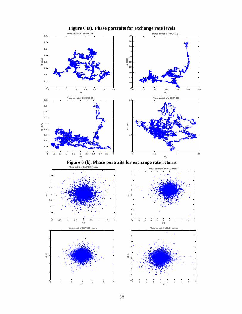
38

Figure 6 (a). Phase portraits for exchange rate levels

0.9 1 1.1 1.2 1.3 1.4 1.5 1.61

1.1

1.2

1.3

1.4

1.5

1.6

1.7

1.8Phase portrait of CAD/USD ER

x(t)

x(t+

1588

)

50 100 150 200 250 300 35080

100

120

140

160

180

200

220

240

260

280Phase portrait of JPY/USD ER

x(t)

x(t+

2555

)

1 1.2 1.4 1.6 1.8 2 2.2 2.4 2.6 2.8 31

1.2

1.4

1.6

1.8

2

2.2

2.4

2.6

2.8Phase portrait of CHF/USD ER

x(t)

x(t+

2573

)

1 1.5 2 2.51

1.5

2

2.5Phase portrait of USD/BP ER

x(t)

x(t+

780)

Figure 6 (b). Phase portraits for exchange rate returns

-2 -1.5 -1 -0.5 0 0.5 1 1.5 2-2

-1.5

-1

-0.5

0

0.5

1

1.5

2Phase portrait of CAD/USD returns

x(t)

x(t+

1)

-6 -5 -4 -3 -2 -1 0 1 2 3 4-6

-5

-4

-3

-2

-1

0

1

2

3

4Phase portrait of JPY/USD returns

x(t)

x(t+

1)

-6 -4 -2 0 2 4 6-6

-4

-2

0

2

4

6Phase portrait of CHF/USD returns

x(t)

x(t+

1)

-4 -3 -2 -1 0 1 2 3 4 5-4

-3

-2

-1

0

1

2

3

4

5Phase portrait of USD/BP returns

x(t)

x(t+

1)

39

Figure 6 (c). Phase portraits for normalized exchange rates

0.92 0.94 0.96 0.98 1 1.02 1.04 1.060.92

0.94

0.96

0.98

1

1.02

1.04

1.06Phase portrait of normalized CAD/USD ER

x(t)

x(t+

43)

0.8 0.85 0.9 0.95 1 1.05 1.1 1.15 1.20.8

0.85

0.9

0.95

1

1.05

1.1

1.15

1.2Phase portrait of normalized JPY/USD ER

x(t)

x(t+

88)

0.85 0.9 0.95 1 1.05 1.1 1.15 1.20.85

0.9

0.95

1

1.05

1.1

1.15

1.2Phase portrait of normalized CHF/USD ER

x(t)

x(t+

73)

0.85 0.9 0.95 1 1.05 1.1 1.15 1.20.85

0.9

0.95

1

1.05

1.1

1.15

1.2Phase portrait of normalized USD/BP ER

x(t)

x(t+

105)

Figure 6 (d). Phase portraits for exchange rate volatilities

0 0.2 0.4 0.6 0.8 1 1.2 1.4 1.6 1.8 20

0.2

0.4

0.6

0.8

1

1.2

1.4

1.6

1.8

2Phase portrait of CAD/USD volatility

x(t)

x(t+

1663

)

0 1 2 3 4 5 60

1

2

3

4

5

6Phase portrait of JPY/USD volatility

x(t)

x(t+

444)

0 1 2 3 4 5 60

1

2

3

4

5

6Phase portrait of CHF/USD volatility

x(t)

x(t+

19)

0 0.5 1 1.5 2 2.5 3 3.5 4 4.5 5

0

0.5

1

1.5

2

2.5

3

3.5

4

4.5

5Phase portrait of USD/BP volatility

x(t)

x(t+

323)

40

Figure 7. Henon Map

-1.5 -1 -0.5 0 0.5 1 1.5-0.4

-0.3

-0.2

-0.1

0

0.1

0.2

0.3

0.4HENON MAP

x

y

Figure 8. Estimation of correlation dimension for Henon map

-2.5 -2 -1.5 -1 -0.5 0 0.5

-7

-6

-5

-4

-3

-2

-1

Correlation dimention estimation, Henon map

log(radius)

log(

corr

elat

ion

inte

gral

)

m = 2

m = 12

-2.5 -2 -1.5 -1 -0.5 0 0.51

1.5

2

2.5

3

3.5

4

4.5

5

5.5

6

Local slopes, Henon map

log(radius)

slop

e

41

Figure 9 (a). Estimation of correlation dimension CAD/USD returns

-8.5 -8 -7.5 -7 -6.5 -6 -5.5 -5 -4.5-16

-14

-12

-10

-8

-6

-4

-2

0Correlation dimention estimation, CAD/USD returns

log(radius)

log(

corr

elat

ion

inte

gral

)

m = 2

m = 12

-8.5 -8 -7.5 -7 -6.5 -6 -5.5 -5 -4.50

2

4

6

8

10

12Local slopes, CAD/USD returns

log(radius)

slop

e

-8.5 -8 -7.5 -7 -6.5 -6 -5.5 -5 -4.5-18

-16

-14

-12

-10

-8

-6

-4

-2

0Correlation dimention estimation, CAD/USD scrambled returns

log(radius)

log(

corr

elat

ion

inte

gral

)

m = 2

m = 12

-8.5 -8 -7.5 -7 -6.5 -6 -5.5 -5 -4.50

2

4

6

8

10

12Local slopes, CAD/USD scrambled returns

log(radius)

slop

e

-2.5 -2 -1.5 -1 -0.5 0 0.5 1-18

-16

-14

-12

-10

-8

-6

-4

-2

0Correlation dimention estimation, CAD/USD returns, GARCH residuals

log(radius)

log(

corr

elat

ion

inte

gral

)

m = 2

m = 12

-2.5 -2 -1.5 -1 -0.5 0 0.5 10

2

4

6

8

10

12

14

16

18Local slopes, CAD/USD returns, GARCH residuals

log(radius)

slop

e

-2.5 -2 -1.5 -1 -0.5 0 0.5 1-18

-16

-14

-12

-10

-8

-6

-4

-2

0Correlation dimention estimation, CAD/USD returns, GARCH scrambled residuals

log(radius)

log(

corr

elat

ion

inte

gral

)

m = 2

m = 12

-2.5 -2 -1.5 -1 -0.5 0 0.5 10

2

4

6

8

10

12

14

16

18Local slopes, CAD/USD returns, GARCH scrambled residuals

log(radius)

slop

e

42

Figure 9 (b). Estimation of correlation dimension JPY/USD returns

-7.5 -7 -6.5 -6 -5.5 -5 -4.5 -4-18

-16

-14

-12

-10

-8

-6

-4

-2

0Correlation dimention estimation, JPY/USD returns

log(radius)

log(

corr

elat

ion

inte

gral

)

m = 2

m = 12

-7.5 -7 -6.5 -6 -5.5 -5 -4.5 -40

1

2

3

4

5

6

7

8

9

10Local slopes, JPY/USD returns

log(radius)

slop

e

-7.5 -7 -6.5 -6 -5.5 -5 -4.5 -4-18

-16

-14

-12

-10

-8

-6

-4

-2

0Correlation dimention estimation, JPY/USD returns, scrambled

log(radius)

log(

corr

elat

ion

inte

gral

)

m = 2

m = 12

-7.5 -7 -6.5 -6 -5.5 -5 -4.5 -40

5

10

15Local slopes, JPY/USD returns, scrambled

log(radius)

slop

e

-2 -1.5 -1 -0.5 0 0.5

-14

-12

-10

-8

-6

-4

-2

Correlation dimention estimation, JPY/USD returns, GARCH residuals

log(radius)

log(

corr

elat

ion

inte

gral

)

m = 2

m = 12

-2 -1.5 -1 -0.5 0 0.50

1

2

3

4

5

6

7

8

9

10

Local slopes, JPY/USD returns, GARCH residuals

log(radius)

slop

e

-2 -1.5 -1 -0.5 0 0.5

-14

-12

-10

-8

-6

-4

-2

Correlation dimention estimation, JPY/USD returns, GARCH residuals, scrambled

log(radius)

log(

corr

elat

ion

inte

gral

)

m = 2

m = 12

-2 -1.5 -1 -0.5 0 0.5

0

1

2

3

4

5

6

7

8

9

10

Local slopes, JPY/USD returns, GARCH residuals, scrambled

log(radius)

slop

e

43

Figure 9 (c). Estimation of correlation dimension CHF/USD returns

-7.5 -7 -6.5 -6 -5.5 -5 -4.5 -4 -3.5-18

-16

-14

-12

-10

-8

-6

-4

-2

0Correlation dimention estimation, CHF/USD returns

log(radius)

log(

corr

elat

ion

inte

gral

)

m = 2

m = 12

-7.5 -7 -6.5 -6 -5.5 -5 -4.5 -4 -3.50

2

4

6

8

10

12

14Local slopes, CHF/USD returns

log(radius)

slop

e

-7.5 -7 -6.5 -6 -5.5 -5 -4.5 -4-18

-16

-14

-12

-10

-8

-6

-4

-2

0Correlation dimention estimation, CHF/USD scrambled returns

log(radius)

log(

corr

elat

ion

inte

gral

)

m = 2

m = 12

-7.5 -7 -6.5 -6 -5.5 -5 -4.5 -40

5

10

15Local slopes, CHF/USD scrambled returns

log(radius)

slop

e

-2.5 -2 -1.5 -1 -0.5 0 0.5 1-18

-16

-14

-12

-10

-8

-6

-4

-2

0Correlation dimention estimation, CHF/USD returns, GARCH residuals

log(radius)

log(

corr

elat

ion

inte

gral

)

m = 2

m = 12

-2.5 -2 -1.5 -1 -0.5 0 0.5 10

2

4

6

8

10

12

14Local slopes, CHF/USD returns, GARCH residuals

log(radius)

slop

e

-2.5 -2 -1.5 -1 -0.5 0 0.5 1-18

-16

-14

-12

-10

-8

-6

-4

-2

0Correlation dimention estimation, CHF/USD returns, GARCH residuals, scrambled

log(radius)

log(

corr

elat

ion

inte

gral

)

m = 2

m = 12

-2.5 -2 -1.5 -1 -0.5 0 0.5 10

2

4

6

8

10

12

14Local slopes, CHF/USD returns, GARCH residuals, scrambled

log(radius)

slop

e

44

Figure 9 (d). Estimation of corre lation dimension USD/BP returns

-7 -6.5 -6 -5.5 -5 -4.5

-14

-12

-10

-8

-6

-4

-2

Correlation dimention estimation, USD/BP returns

log(radius)

log(

corr

elat

ion

inte

gral

)

m = 2

m = 12

-7 -6.5 -6 -5.5 -5 -4.5

1

2

3

4

5

6

Local slopes, USD/BP returns

log(radius)

slop

e

-7.5 -7 -6.5 -6 -5.5 -5 -4.5 -4-18

-16

-14

-12

-10

-8

-6

-4

-2

0Correlation dimention estimation, USD/BP scrambled returns

log(radius)

log(

corr

elat

ion

inte

gral

)

m = 2

m = 12

-7.5 -7 -6.5 -6 -5.5 -5 -4.5 -40

2

4

6

8

10

12Local slopes, USD/BP scrambled returns

log(radius)

slop

e

-2.5 -2 -1.5 -1 -0.5 0 0.5 1-18

-16

-14

-12

-10

-8

-6

-4

-2

0Correlation dimention estimation, USD/BP returns, GARCH residuals

log(radius)

log(

corr

elat

ion

inte

gral

)

m = 2

m = 12

-2.5 -2 -1.5 -1 -0.5 0 0.5 10

1

2

3

4

5

6

7

8Local slopes, USD/BP returns, GARCH residuals

log(radius)

slop

e

-2.5 -2 -1.5 -1 -0.5 0 0.5 1-18

-16

-14

-12

-10

-8

-6

-4

-2

0Correlation dimention estimation, USD/BP returns, GARCH residuals, scrambled

log(radius)

log(

corr

elat

ion

inte

gral

)

m = 2

m = 12

-2.5 -2 -1.5 -1 -0.5 0 0.5 10

5

10

15Local slopes, USD/BP returns, GARCH residuals, scrambled

log(radius)

slop

e

45

Figure 10 (a). Estimation of correlation dimension for CAD/USD normalized ER

-6.5 -6 -5.5 -5 -4.5 -4 -3.5

-14

-12

-10

-8

-6

-4

-2

Correlation dimention estimation, CAD/USD normalized ER

log(radius)

log(

corr

elat

ion

inte

gral

)

m = 2

m = 12

-6.5 -6 -5.5 -5 -4.5 -4 -3.50

1

2

3

4

5

6

7

8

9

10Local slopes, CAD/USD normalized ER

log(radius)

slop

e

-7 -6.5 -6 -5.5 -5 -4.5 -4 -3.5 -3-18

-16

-14

-12

-10

-8

-6

-4

-2

0Correlation dimension estimation, CAD/USD normalized ER, scrambled

log(radius)

log(

corr

elat

ion

inte

gral

)

m = 2

m = 12

-7 -6.5 -6 -5.5 -5 -4.5 -4 -3.5 -30

2

4

6

8

10

12

14

16Local slopes, CAD/USD normalized ER, scrambled

log(radius)

slop

e

-6.5 -6 -5.5 -5 -4.5 -4 -3.5 -14

-12

-10

-8

-6

-4

-2

log(radius)

log(

corr

elat

ion

inte

gral

)

-6.5 -6 -5.5 -5 -4.5 -4 -3.5 1

2

3

4

5

6

7 Local slopes, CAD/USD normalized ER, without correction

log(radius)

slop

e

Correlation dimension estimation, CAD/USD normalized ER, without correction

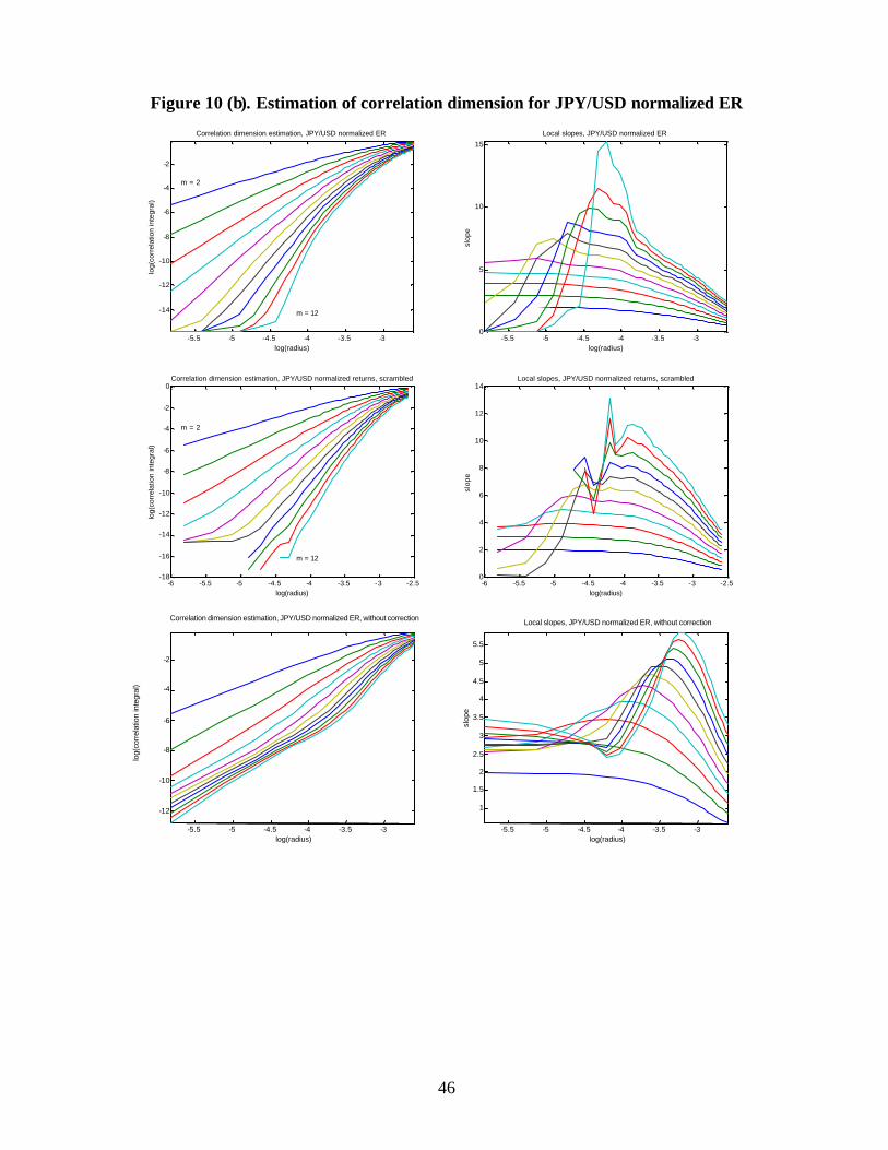
46

Figure 10 (b). Estimation of correlation dimension for JPY/USD normalized ER

-5.5 -5 -4.5 -4 -3.5 -3

-14

-12

-10

-8

-6

-4

-2

Correlation dimension estimation, JPY/USD normalized ER

log(radius)

log(

corr

elat

ion

inte

gral

)

m = 2

m = 12

-5.5 -5 -4.5 -4 -3.5 -30

5

10

15Local slopes, JPY/USD normalized ER

log(radius)

slop

e

-6 -5.5 -5 -4.5 -4 -3.5 -3 -2.5-18

-16

-14

-12

-10

-8

-6

-4

-2

0Correlation dimension estimation, JPY/USD normalized returns, scrambled

log(radius)

log(

corr

elat

ion

inte

gral

)

m = 2

m = 12

-6 -5.5 -5 -4.5 -4 -3.5 -3 -2.50

2

4

6

8

10

12

14Local slopes, JPY/USD normalized returns, scrambled

log(radius)

slop

e

-5.5 -5 -4.5 -4 -3.5 -3 -12

-10

-8

-6

-4

-2

Correlation dimension estimation, JPY/USD normalized ER, without correction

log(radius)

log(

corr

elat

ion

inte

gral

)

-5.5 -5 -4.5 -4 -3.5 -3 1

1.5 2

2.5 3

3.5 4

4.5 5

5.5 Local slopes, JPY/USD normalized ER, without correction

log(radius)

slop

e

47

Figure 10 (c). Estimation of correlation dimension for CHF/USD normalized ER

-5.5 -5 -4.5 -4 -3.5 -3

-14

-12

-10

-8

-6

-4

-2

Correlation dimension estimation, CHF/USD normalized ER

log(radius)

log(

corr

elat

ion

inte

gral

)

m = 2

m = 12

-5.5 -5 -4.5 -4 -3.5 -30

1

2

3

4

5

6

7

8

9

Local slopes, CHF/USD normalized ER

log(radius)

slop

e

-5.5 -5 -4.5 -4 -3.5 -3

-14

-12

-10

-8

-6

-4

-2

Correlation dimension estimation, CHF/USD normalized ER, scrambled

log(radius)

log(

corr

elat

ion

inte

gral

)

m = 2

m = 12

-5.5 -5 -4.5 -4 -3.5 -30

2

4

6

8

10

Local slopes, CHF/USD normalized ER, scrambled

log(radius)

slop

e

-5.5 -5 -4.5 -4 -3.5 -3

-12

-10

-8

-6

-4

-2

Correlation dimension estimation, CHF/USD normalized ER, without correction

log(radius)

log(

corr

elat

ion

inte

gral

)

-5.5 -5 -4.5 -4 -3.5 -3 1

2

3

4

5

6

Local slopes, CHF/USD normalized ER, without correction

log(radius)

slop

e

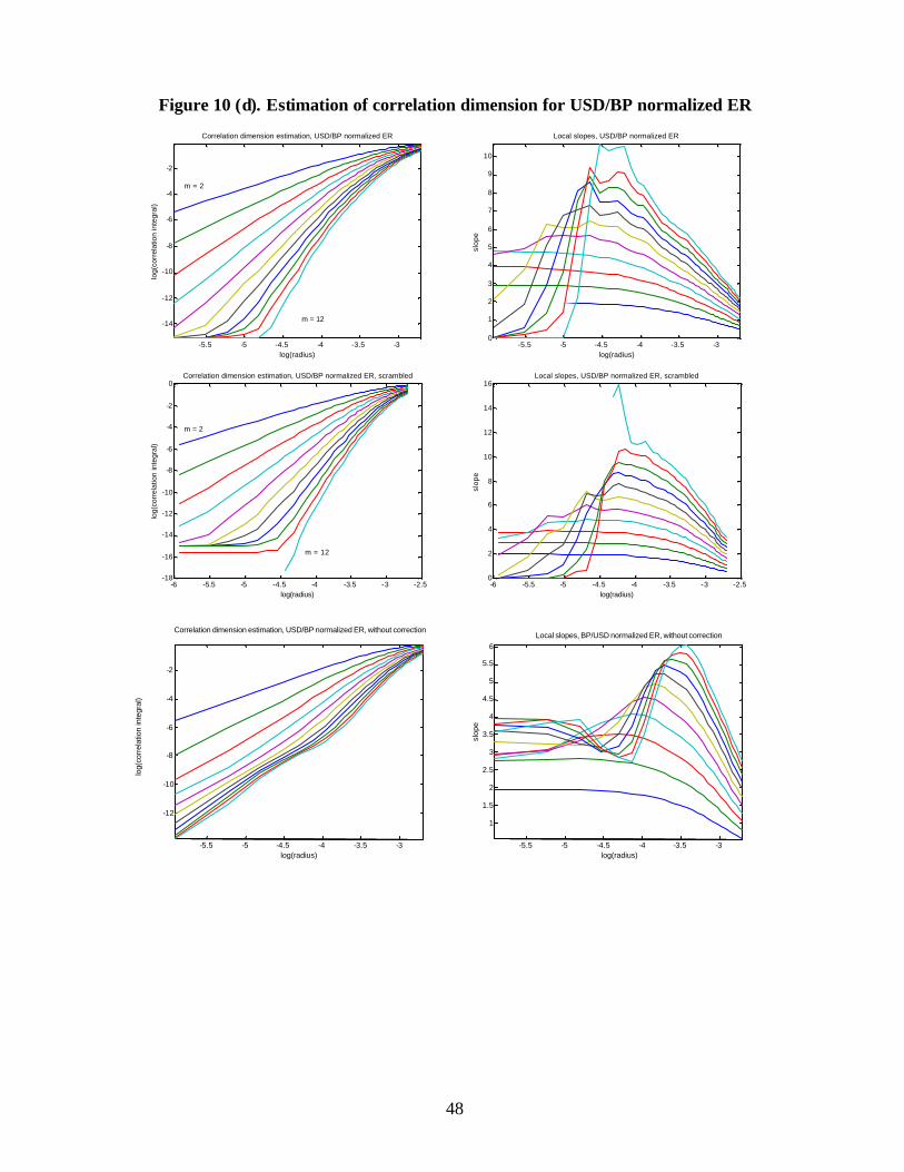
48

Figure 10 (d). Estimation of correlation dimension for USD/BP normalized ER

-5.5 -5 -4.5 -4 -3.5 -3

-14

-12

-10

-8

-6

-4

-2

Correlation dimension estimation, USD/BP normalized ER

log(radius)

log(

corr

elat

ion

inte

gral

)

m = 2

m = 12

-5.5 -5 -4.5 -4 -3.5 -30

1

2

3

4

5

6

7

8

9

10

Local slopes, USD/BP normalized ER

log(radius)

slop

e

-6 -5.5 -5 -4.5 -4 -3.5 -3 -2.5-18

-16

-14

-12

-10

-8

-6

-4

-2

0Correlation dimension estimation, USD/BP normalized ER, scrambled

log(radius)

log(

corr

elat

ion

inte

gral

)

m = 2

m = 12

-6 -5.5 -5 -4.5 -4 -3.5 -3 -2.50

2

4

6

8

10

12

14

16Local slopes, USD/BP normalized ER, scrambled

log(radius)

slop

e

-5.5 -5 -4.5 -4 -3.5 -3

-12

-10

-8

-6

-4

-2

Correlation dimension estimation, USD/BP normalized ER, without correction

log(radius)

log(

corr

elat

ion

inte

gral

)

-5.5 -5 -4.5 -4 -3.5 -3 1

1.5 2

2.5 3

3.5 4

4.5 5

5.5 6

Local slopes, BP/USD normalized ER, without correction

log(radius)

slop

e

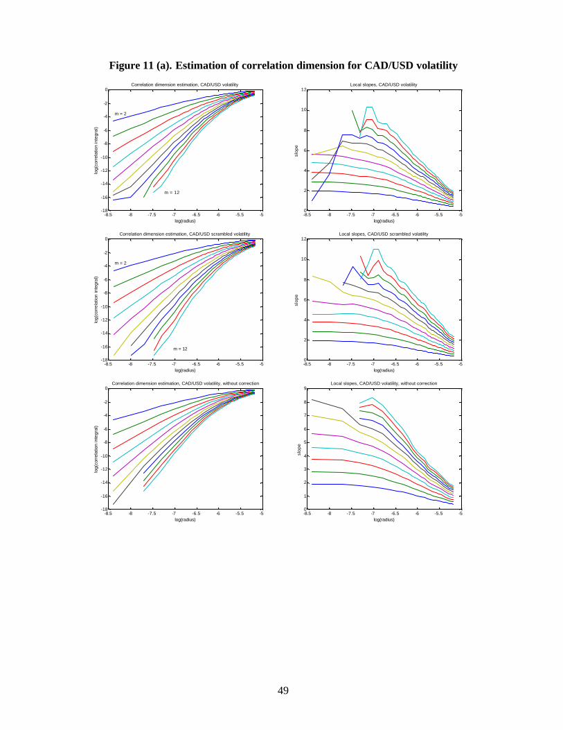
49

Figure 11 (a). Estimation of correlation dimension for CAD/USD volatility

-8.5 -8 -7.5 -7 -6.5 -6 -5.5 -5-18

-16

-14

-12

-10

-8

-6

-4

-2

0Correlation dimension estimation, CAD/USD volatility

log(radius)

log(

corr

elat

ion

inte

gral

)

m = 2

m = 12

-8.5 -8 -7.5 -7 -6.5 -6 -5.5 -50

2

4

6

8

10

12Local slopes, CAD/USD volatility

log(radius)

slop

e

-8.5 -8 -7.5 -7 -6.5 -6 -5.5 -5-18

-16

-14

-12

-10

-8

-6

-4

-2

0Correlation dimension estimation, CAD/USD scrambled volatility

log(radius)

log(

corr

elat

ion

inte

gral

)

m = 2

m = 12

-8.5 -8 -7.5 -7 -6.5 -6 -5.5 -50

2

4

6

8

10

12Local slopes, CAD/USD scrambled volatility

log(radius)

slop

e

-8.5 -8 -7.5 -7 -6.5 -6 -5.5 -5-18

-16

-14

-12

-10

-8

-6

-4

-2

0Correlation dimension estimation, CAD/USD volatility, without correction

log(radius)

log(

corr

elat

ion

inte

gral

)

-8.5 -8 -7.5 -7 -6.5 -6 -5.5 -50

1

2

3

4

5

6

7

8

9Local slopes, CAD/USD volatility, without correction

log(radius)

slop

e

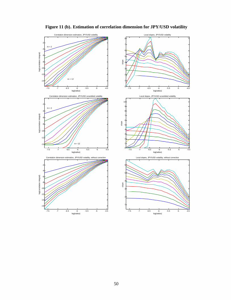
50

Figure 11 (b). Estimation of correlation dimension for JPY/USD volatility

-7.5 -7 -6.5 -6 -5.5 -5 -4.5

-14

-12

-10

-8

-6

-4

-2

Correlation dimension estimation, JPY/USD volatility

log(radius)

log(

corr

elat

ion

inte

gral

)

m = 2

m = 12

-7.5 -7 -6.5 -6 -5.5 -5 -4.50

1

2

3

4

5

6

7

8

Local slopes, JPY/USD volatility

log(radius)

slop

e

-7.5 -7 -6.5 -6 -5.5 -5 -4.5

-14

-12

-10

-8

-6

-4

-2

Correlation dimension estimation, JPY/USD scrambled volatility

log(radius)

log(

corr

elat

ion

inte

gral

)

m = 2

m = 12

-7.5 -7 -6.5 -6 -5.5 -5 -4.50

1

2

3

4

5

6

7

8

9

10

Local slopes, JPY/USD scrambled volatility

log(radius)

slop

e

-7.5 -7 -6.5 -6 -5.5 -5 -4.5

-16

-14

-12

-10

-8

-6

-4

-2

Correlation dimension estimation, JPY/USD volatility, without correction

log(radius)

log(

corr

elat

ion

inte

gral

)

-7.5 -7 -6.5 -6 -5.5 -5 -4.5

1

2

3

4

5

6

Local slopes, JPY/USD volatility, without correction

log(radius)

slop

e

51

Figure 11 (c). Estimation of correlation dimension for CHF/USD volatility

-7.5 -7 -6.5 -6 -5.5 -5 -4.5

-14

-12

-10

-8

-6

-4

-2

Correlation dimension estimation, CHF volatility

log(radius)

log(

corr

elat

ion

inte

gral

)

m = 2

m = 12

-7.5 -7 -6.5 -6 -5.5 -5 -4.50

1

2

3

4

5

6

7

8

9Local slopes, CHF volatility

log(radius)

slop

e

-7.5 -7 -6.5 -6 -5.5 -5 -4.5

-14

-12

-10

-8

-6

-4

-2

Correlation dimension estimation, CHF scrambled volatility

log(radius)

log(

corr

elat

ion

inte

gral

)

m = 2

m = 12

-7.5 -7 -6.5 -6 -5.5 -5 -4.50

1

2

3

4

5

6

7

8

9

Local slopes, CHF scrambled volatility

log(radius)

slop

e

-7.5 -7 -6.5 -6 -5.5 -5 -4.5

-14

-12

-10

-8

-6

-4

-2

Correlation dimension estimation, CHF/USD volatility, without correction

log(radius)

log(

corr

elat

ion

inte

gral

)

-7.5 -7 -6.5 -6 -5.5 -5 -4.50

1

2

3

4

5

6

7

8

Local slopes, CHF/USD volatility, without correction

log(radius)

slop

e

52

Figure 11 (d). Estimation of correlation dimension for USD/BP volatility

-7.5 -7 -6.5 -6 -5.5 -5

-16

-14

-12

-10

-8

-6

-4

-2

Correlation dimension estimation. USD/BP

log(radius)

log(

corr

elat

ion

inte

gral

)

m = 2

m = 12

-7.5 -7 -6.5 -6 -5.5 -5

1

2

3

4

5

6

7

8

9

Local slopes, USD/BP volatility

log(radius)

slop

e

-8 -7.5 -7 -6.5 -6 -5.5 -5 -4.5-18

-16

-14

-12

-10

-8

-6

-4

-2

0Correlation dimension estimation, USD/BP scrambled volatility

log(radius)

log(

corr

elat

ion

inte

gral

)

m = 2

m = 12

-8 -7.5 -7 -6.5 -6 -5.5 -5 -4.50

5

10

15Local slopes, USD/BP scrambled volatility

log(radius)

slop

e

-5.5 -5 -4.5 -4 -3.5 -3-10

-9

-8

-7

-6

-5

-4

-3

-2

-1

Correlation dimension estimation, USD/BP volatility, without correction

log(radius)

log(

corr

elat

ion

inte

gral

)

-5.5 -5 -4.5 -4 -3.5 -30.5

1

1.5

2

2.5

3

3.5

4

4.5

5

Local slopes, USD/BP volatility, without correction

log(radius)

slop

e

53

Figure 12. Maximum Lyapunov exponent estimation, Henon map

0 2 4 6 8 10 12 14 16 18 20

-7

-6

-5

-4

-3

-2

-1

0

L1 estimation, Henon map

# of separation steps

aver

. log

of d

ist.

0 2 4 6 8 10 12 14 16 18 200

0.05

0.1

0.15

0.2

0.25

0.3

0.35

0.4

0.45Local slopes, Henon map

# of separation steps

slop

e

54

Figure 13. Maximum Lyapunov exponent estimation, JPY/USD returns

0 2 4 6 8 10 12 14 16 18 20-8

-7.5

-7

-6.5

-6

-5.5

-5

-4.5

-4L1 estimation, JPY/USD returns

# of separation steps

aver

. log

of d

ist.

0 2 4 6 8 10 12 14 16 18 20-1

-0.5

0

0.5

1

1.5

2

2.5

3Local slopes, JPY/USD returns

# of separation steps

slop

e

0 2 4 6 8 10 12 14 16 18 20-8

-7.5

-7

-6.5

-6

-5.5

-5

-4.5

-4

-3.5L1 estimation, JPY/USD scrambled returns

# of separation steps

aver

. log

of d

ist.

0 2 4 6 8 10 12 14 16 18 20-0.5

0

0.5

1

1.5

2

2.5Local slopes, JPY/USD scrambled returns

# of separation steps

slop

e

0 2 4 6 8 10 12 14 16 18 20-5

-4

-3

-2

-1

0

1

2L1 estimation, JPY/USD GARCH filtered returns

# of separation steps

aver

. log

of d

ist.

0 2 4 6 8 10 12 14 16 18 20-0.5

0

0.5

1

1.5

2

2.5

3

3.5

4

4.5Local slopes, JPY/USD GARCH filtered returns

# of separation steps

slop

e

0 2 4 6 8 10 12 14 16 18 20-3

-2.5

-2

-1.5

-1

-0.5

0

0.5

1

1.5L1 estimation, JPY/USD GARCH filtered returns, scrambled

# of separation steps

aver

. log

of d

ist.

0 2 4 6 8 10 12 14 16 18 20-0.5

0

0.5

1

1.5

2

2.5Local slopes, JPY/USD GARCH filtered returns, scrambled

# of separation steps

slop

e

55

Figure 14. MLE estimation, JPY/USD normalized ER and volatility

0 2 4 6 8 10 12 14 16 18 20-8

-7

-6

-5

-4

-3

-2L1 estimation, JPY/USD normalized ER

# of separation steps

aver

. log

of d

ist.

0 2 4 6 8 10 12 14 16 18 20-0.5

0

0.5

1

1.5

2

2.5

3Local slopes, JPY/USD normalized ER

# of separation steps

slop

e

0 2 4 6 8 10 12 14 16 18 20-7.5

-7

-6.5

-6

-5.5

-5

-4.5

-4

-3.5

-3

-2.5L1 estimation, JPY/USD normalized ER, scrambled

# of separation steps

aver

. log

of d

ist.

0 2 4 6 8 10 12 14 16 18 20-0.5

0

0.5

1

1.5

2

2.5

3

3.5

4Local slopes, JPY/USD normalized ER, scrambled

# of separation steps

slop

e

0 2 4 6 8 10 12 14 16 18 20-8.5

-8

-7.5

-7

-6.5

-6

-5.5

-5

-4.5

-4L1 estimation, JPY/USD volatility

# of separation steps

aver

. log

of d

ist.

0 2 4 6 8 10 12 14 16 18 20

-1

-0.5

0

0.5

1

1.5

2

2.5

3

3.5Local slopes, JPY/USD volatility

# of separation steps

slop

e

0 2 4 6 8 10 12 14 16 18 20-8.5

-8

-7.5

-7

-6.5

-6

-5.5

-5

-4.5

-4L1 estimation, JPY/USD volatility, scrambled

# of separation steps

aver

. log

of d

ist.

0 2 4 6 8 10 12 14 16 18 20-0.5

0

0.5

1

1.5

2

2.5Local slopes, JPY/USD volatility, scrambled

# of separation steps

slop

e