Embed Size (px)
Citation preview
Nonlinear Waves Lecture Notes(G14 NWA/2)
Dr R H TewDivision of Applied Mathematics, School of Mathematical Sciences,University of Nottingham, University Park, Nottingham, NG7 2RD.
Autumn Semester 2005
Contents
1 Linear Wave Theory & Other Background 41.1 Linear wave equations . . . . . . . . . . . . . 41.2 Other equations . . . . . . . . . . . . . . . . . 41.3 Dispersion relation . . . . . . . . . . . . . . . 51.4 Group velocity . . . . . . . . . . . . . . . . . 51.5 Lagrangian mechanics . . . . . . . . . . . . . 6
1.5.1 The Euler-Lagrange equations . . . . 61.5.2 Hamiltonian mechanics . . . . . . . . 7
1.6 Nonlinearity . . . . . . . . . . . . . . . . . . . 8
2 Integrable Systems 92.1 The solitary wave solution . . . . . . . . . . . 92.2 The classic integrable systems . . . . . . . . . 10
2.2.1 KdV . . . . . . . . . . . . . . . . . . . 102.2.2 NLS . . . . . . . . . . . . . . . . . . . 102.2.3 NLS – dispersion relations . . . . . . . 102.2.4 NLS – special solutions . . . . . . . . 112.2.5 SG . . . . . . . . . . . . . . . . . . . . 122.2.6 SG – Kink solution . . . . . . . . . . . 132.2.7 SG – Breather solution . . . . . . . . 142.2.8 SG – 2-soliton solution . . . . . . . . . 142.2.9 Others . . . . . . . . . . . . . . . . . . 15
2.3 2-soliton solution - Backlund Transformation 152.3.1 KdV - History . . . . . . . . . . . . . 152.3.2 Example: (nothing→soliton) . . . . . 162.3.3 Example: (1-soliton→2-soliton) . . . . 172.3.4 Backlund Transformation for SG . . . 172.3.5 Application of BT for SG . . . . . . . 18
2.4 Lax pairs . . . . . . . . . . . . . . . . . . . . 182.4.1 Lax pair for KdV . . . . . . . . . . . . 192.4.2 NLS . . . . . . . . . . . . . . . . . . . 20
2.5 Conserved quantities . . . . . . . . . . . . . . 202.5.1 KdV - motivation . . . . . . . . . . . 202.5.2 KdV-theory . . . . . . . . . . . . . . . 212.5.3 NLS . . . . . . . . . . . . . . . . . . . 21
3 Methods – for nonintegrable systems 223.1 Easy example (NLS) . . . . . . . . . . . . . . 223.2 Harder example – collective variables (NLS) . 223.3 Forcing and damping in SG . . . . . . . . . . 24
3.3.1 Ground States . . . . . . . . . . . . . 243.3.2 Kink solution . . . . . . . . . . . . . . 25
3.3.3 Behaviour at intermediate times . . . 263.3.4 Summary – Power Balancing . . . . . 26
3.4 Nonsymmetric Klein-Gordon breather . . . . 263.5 Numerical Solution of Equations . . . . . . . 28
4 Applications 294.1 Electrical Transmission Lines . . . . . . . . . 29
4.1.1 Aside . . . . . . . . . . . . . . . . . . 304.1.2 Onto KdV . . . . . . . . . . . . . . . . 304.1.3 Regularising long wave equations . . . 314.1.4 Comparison of solitary wave solutions 33
4.2 Fibre-optic Cables . . . . . . . . . . . . . . . 344.3 Water Waves . . . . . . . . . . . . . . . . . . 35
4.3.1 Linear Theory . . . . . . . . . . . . . 364.3.2 Nonlinear Theory . . . . . . . . . . . . 374.3.3 Intepretation of Results . . . . . . . . 39
4.4 Long Josephson junctions . . . . . . . . . . . 394.4.1 Current–Voltage Characteristics . . . 41
4.5 Waves in nonlinear diffusion problems . . . . 414.5.1 Fisher-KPP equation . . . . . . . . . . 444.5.2 Multiple waves . . . . . . . . . . . . . 44
Format of Exam:G14 NW2 (15 credits): one 21
2-hour paper, attempt
3 out of 4 questionsG14 NWA (20 credits): one 3-hour paper, attempt4 out of 5 questions
Syllabus for G14 NW2 (useful for Revision)(i) Linear wave theory & background(ii) Integrable systems: 1-soliton solution, hierarchiesof conserved quantities, Lax pair, 2-soliton solution,envelope solutions (bright and dark), kink solutions,breather solutions. Examples: KdV, NLS & SG(iii) Methods for nonintegrable systems: perturbationtheory, large-time asymptotics, stability of solitons, power-balancing, numerical solution of equations(iv) Applications: electrical transmission lines, fibre-optic cables, water waves, Josephson junctions, nonlin-ear diffusion equations
1
G14 NWA/2 Nonlinear Waves 2
Module Philosophy Lesson 1
Lesson 1
Ideally the scientific process goes:
(1) physical process/scientific experiment
(2) set of mathematical equations
(3) solution of equations
(4) interpret results
However, we are mathematicians and probably most comfortable with the stage (2) → (3).
This module will also try to cover some of the processes involved in stages (1) → (2) and (3) → (4).
This module is designed to be fairly self-sufficient, no knowledge of PDEs, functional analysis, electric cir-
cuit theory, fibre-optic cables, superconductors, water waves, perturbation theory, etc., will be assumed,
(although I hope you will pick some up by the end of the module).
Lesson 2
There is a nice neat theory of constant coefficient linear ODEs–[hopefully you have met this]–solutions have
the form C0veλt. You may also have met a nice neat theory of second order linear PDEs classifying them
as elliptic, parabolic or hyperbolic.
But a nice neat theory of nonlinear PDEs does not exist. Instead this module shows some typical
behaviours which may be observed, and ways of analysing them. There are other more exotic solutions
out there being discovered all the time–this is an area of current active research.
[Not everything fits into neat categories, you set up a set of boxes and then soon find something which straddles two boxes,
or you have to keep creating new categories].
[If you are doing the 20 credit option (C) and there are things which interest you and you want to know more about, you
can do it as a project - come and talk and I’ll point you in the right direction to get started.]
G14 NWA/2 Nonlinear Waves 3
1 Linear Wave Theory & Other Background
1.1 Linear wave equations
The simplest wave equation
ut + cux = 0
has general solution u = f(x− ct) where f(·) is determined by initial conditions.
utt − c2uxx = 0
is usually referred to as ‘the wave equation’ has general solution u(x, t) = f(x− ct) + g(x+ ct)
–a linear superposition of two waves, one right-propagating and the other left-propagating.
An alternative solution method uses separation of variables, and seeks a solution in the form u(x, t) =
X(x)T (t). This leads to X ′′/X = T ′′/c2T = −k2, a constant; since X ′′/X is independent of t and T ′′/c2T
is independent of x, k must be independent of x and t. Thus we have the solution
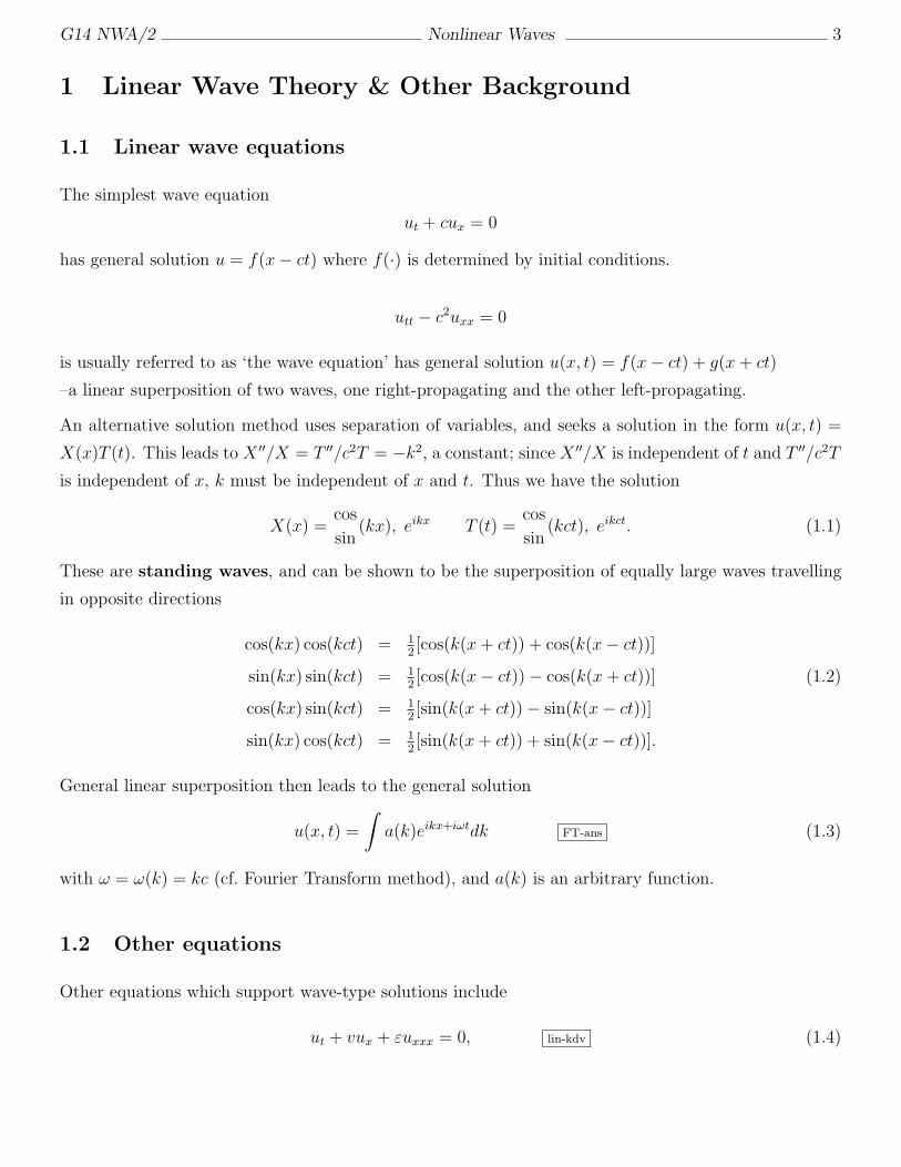
X(x) =cos
sin(kx), eikx T (t) =
cos
sin(kct), eikct. (1.1)
These are standing waves, and can be shown to be the superposition of equally large waves travelling
in opposite directions
cos(kx) cos(kct) = 12[cos(k(x+ ct)) + cos(k(x− ct))]
sin(kx) sin(kct) = 12[cos(k(x− ct))− cos(k(x+ ct))] (1.2)
cos(kx) sin(kct) = 12[sin(k(x+ ct))− sin(k(x− ct))]
sin(kx) cos(kct) = 12[sin(k(x+ ct)) + sin(k(x− ct))].
General linear superposition then leads to the general solution
u(x, t) =
∫
a(k)eikx+iωtdk FT-ans (1.3)
with ω = ω(k) = kc (cf. Fourier Transform method), and a(k) is an arbitrary function.
1.2 Other equations
Other equations which support wave-type solutions include
ut + vux + εuxxx = 0, lin-kdv (1.4)
G14 NWA/2 Nonlinear Waves 4
if we try u(x, t) = f(x− ct) = f(z) we find −cf + vf + εf ′′ = K;
in the case K = 0 this has a solution of the form f = B0 cos(z√
(v − c)/ε) +B1 sin(z√
(v − c)/ε)
or f = Aeikz with k2 = (v − c)/ε, or u = Aeikx−ikct with c = v − εk2.
An alternative approach is to try a solution of the form (1.3) then (1.4) becomes
∫
a(k)eikx+iωt[
iω + vik − ik3]
dk = 0 (1.5)
thus for the equation to be satisfied, we need ω = k3 − vk.
1.3 Dispersion relation
A standard technique to investigate the possibility of wave propagation in a system is to assume a solution
of the form u = eikx+iωt and see how the temporal frequency ω depends on the spatial wave number k.
Such a relation ω = ω(k) is called the dispersion relation.
If ω is real then this is the frequency which the spatial mode eikx oscillates at.
If ω = −iγ with γ > 0 then the solution has the form u = eikxeγt and the mode eikx is unstable, its
amplitude growing exponentially.
If ω = +iγ with γ > 0 then the solution has the form u = eikxe−γt and the mode eikx is damped out in
the system, its amplitude decaying exponentially.
Example
For the telegraph equation utt = uxx + βu, the dispersion relation is ω2 = k2 − β. However the interpre-
tation of this is the important part.
If β < 0 then waves exist for all k and waves with higher wavenumbers having higher frequencies. But
if β > 0 then waves with k <√β have real frequency, but when k >
√β, ω is purely imaginary and so
u = eikx+γt with γ = ±iω, so there is a wave whose amplitude grows exponentially–an unstable situation.
Such equations are usually termed ‘ill-posed’, although solutions with no high frequency component can
still be found.
1.4 Group velocity
In several of the examples quoted above, we have seen that the quantity ω/k gives the speed of translation
of the wave - this is known as the phase velocity.
Another important concept in more complicated waves is that of group velocity.
G14 NWA/2 Nonlinear Waves 5
Suppose we have two waves ua, ub with similar wavenumbers k = k0 ± k1 and similar frequencies ω =
ω0 ± ω1 with k1, ω1 both small since ω = ω(k) is smooth. Then
ua = eikax−iωat = ei(k0+k1)x−i(ω0+ω1)t travelling at speed ca =ωa
ka=
(ω0 + ω1)
(k0 + k1)
ub = eikbx−iωbt = ei(k0−k1)x−i(ω0−ω1)t travelling at speed cb =ωb
kb=
(ω0 − ω1)
(k0 − k1)(1.6)
then the combination u1 + u2 can be written
u1 + u2 = eik0x−iω0t(eik1x−iω1t + e−ik1x+iω1t) (1.7)
so we see a wave like ua, ub travelling at speed c = ω0/k0 modulated with a wave of small wavenumber
(long wave length k1) which is travelling at speed
vgroup =ω1
k1=
ωa − ωb
ka − kb=
dω
dk. (1.8)
This is known as the group velocity. c = ω/k is known as the phase velocity.
1.5 Lagrangian mechanics
In many examples we shall make use of the Hamiltonian/Lagrangian formulation of the equations of
motion. If {qk}Nk=1 are the coordinate variables, and the kinetic and potential energies are given by
T = T ({ Úqk}) =N∑
k=1
12Úq2k (typically), V = V ({qk}) (1.9)
then the Lagrangian is given by L( Úqk, qk) = T − V and the equations of motion are derived by applying:
1.5.1 The Euler-Lagrange equations
The Action is calculated by integrating the Lagrangian over time,
S[q] =
∫ t1
t0
L(q(t), Úq(t)) dt. (1.10)
This equations of motion can then be found by use of a variational principle, namely by setting δSδq
= 0,
determining critical points of S[q].
Formally we wish to construct the first two terms in a Taylor series for S[q]
S[q + εr] = S[q] + εrS ′[q] +O(ε2), (1.11)
G14 NWA/2 Nonlinear Waves 6
where S ′[q] = δSδq
. We can form this by
S[q + εr] =
∫ t1
t0
L(q + εr, Úq + ε Úr) dt (1.12)
=
∫ t1
t0
L(q, Úq) + εr∂L
∂q+ ε Úr
∂L
∂ Úqdt+O(ε2) dt
=
∫ t1
t0
L(q, Úq) dt+ ε
∫ t1
t0
r∂L
∂qdt+ ε
[
r∂L
∂ Úq
]t1
t0
− ε
∫ t1
t0
rd
dt
(
∂L
∂ Úq
)
dt+O(ε2)
= S[q] + ε
∫ t1
t0
r
(
∂L
∂q− d
dt
(
∂L
∂ Úq
))
dt+O(ε2)
assuming[
r ∂L∂ Úq
]t1
t0= 0; then
δS
δqr = S ′[q]r =
∫ t1
t0
(
∂L
∂q− d
dt
(
∂L
∂ Úq
))
r(t) dt.
By assuming S ′[q]r = 0 for all possible choices of r(t), we find the Euler-Lagrange equations ∂L∂q
−ddt
(
∂L∂ Úq
)
= 0.
The variational derivative δSδq
is also known as a Frechet derivative.
In systems where there are many independent variables, the above result generalises to
d
dt
(
∂L
∂ Úqk
)
=∂L
∂qk, k = 1, 2, . . . , N. (1.13)
Ex: Show that for L = L(q, Úq, q), the Euler-Lagrange equation is
∂L
∂q− d
dt
∂L
∂ Úq+
d2
dt2∂L
∂q= 0.
1.5.2 Hamiltonian mechanics
In the Hamiltonian formulation generalised momenta pk are used in place of Úqk, these are determined by
pk =∂L
∂qk. (1.14)
The Hamiltonian is then defined by
H =N∑
k=1
pk Úqk − L =N∑
k=1
Úqk∂L
∂qk− L (1.15)
(this is usually equal to the total energy in the system). The Equations of motion can then be found by
Úqk =∂H
∂pk, Úpk = −∂H
∂qk. (1.16)
G14 NWA/2 Nonlinear Waves 7
For continuous systems, all quantities are replaced by densities, for example the Lagrangian density is
L = L(qt(x, t), q(x, t)) = T (qt(x, t))− V(q(x, t)) = 12q2t − 1
2q2 (for example) (1.17)
then the Lagrangian/Hamiltonian is the integral of the corresponding density over all space,
L =
∫
L dx, H =
∫
H dx. (1.18)
The equations of motion (which are now PDEs) are then
qt(x, t) =δH
δp(x, t), pt(x, t) =
δH
δq(x, t)=
∂H
∂q− ∂
∂x
∂H
∂qx+
∂2
∂x2
∂H
∂qxx− . . . (1.19)
[see Goldstein for more details].
This formalism has been generalised to systems in which there is only one time derivative by
∂u
∂t=
∂
∂x
(
δHδu
)
. (1.20)
For example KdV can be generated by
H = u3 + 12u2x. (1.21)
Alternatively, one can introduce a new variable ψ such that ψx = u and then
L = −12ψtψx − ψ3
x +12ψ2xx (1.22)
produces ut + 6uux + uxxx = 0.
1.6 Nonlinearity
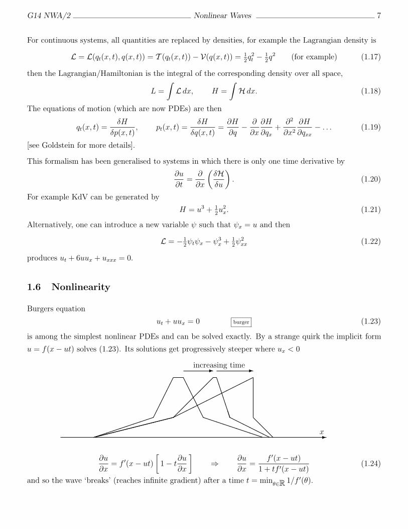
Burgers equation
ut + uux = 0 burger (1.23)
is among the simplest nonlinear PDEs and can be solved exactly. By a strange quirk the implicit form
u = f(x− ut) solves (1.23). Its solutions get progressively steeper where ux < 0
-x
increasing time
°°°°°°°°°¡¡¡¡¡¡ A
AAAAAPPPPPPPPP
-
¸¸¸¸¸¸¸¸¸¸¸¸
B
BBBBBBHHHHHH
-
¸¸¸¸¸¸¸¸¸¸¸¸¨¨¨¨¨¨¨¨¨¨¨¨
@@
@
∂u
∂x= f ′(x− ut)
[
1− t∂u
∂x
]
⇒ ∂u
∂x=
f ′(x− ut)
1 + tf ′(x− ut)(1.24)
and so the wave ‘breaks’ (reaches infinite gradient) after a time t = minθ∈R 1/f ′(θ).
G14 NWA/2 Nonlinear Waves 8
2 Integrable Systems
We have seen that linear waves often suffer from dispersion, so spread out, and that nonlinearity can
cause waves to steepen, so in systems which have both effects, there might be waves of permanent form
in which these two effects exactly balance.
This is indeed the case, and in some systems such waves pass through each other without suffering any
permanent change in form. These systems are called integrable. Integrable systems are in some sense
solvable. We would like to be able to find the solution u(x, t) of a problem, given a PDE, for an arbitrary
set of initial conditions u(x, 0) and some boundary data. For integrable systems there is a theory which
enables this to be carried out (the calculations are often hideous but technically possible).
2.1 The solitary wave solution
Simply look for a travelling wave: assume there is a solution of the form u(z) = u(x − ct) for some
constant speed c (as yet undetermined), converting the PDE into an ODE which is easier to solve
Eg: the Boussinesq equation utt = uxx + (u2)xx + uxxxx becomes
c2u′′(z) = u′′ + (u2)′′ + u′′′′ (2.1)
integrate twice
(c2 − 1)u = u2 + u′′ −K −Mz (2.2)
(assume M = 0 for simplicity),
×u′ and integrate again
(c2 − 1)uu′ = u2u′ + u′′u′ −Ku′
12(c2 − 1)u2 = 1
3u3 + 1
2(u′)2 −Ku− L (2.3)
du
dz= ±
√
2L+ 2Ku+ (c2−1)u2 − 23u3 ⇒ z − z0 = ±
∫
du√
2L+ 2Ku+ (c2−1)u2 − 23u3
.
If u, u′ → 0 as z → ±∞, then L = 0 = K and u = 32(c2−1)sech2(1
2
√c2−1 z)
Defn: a solitary wave is a localised wave that propagates along one spatial direction only, with unde-
formed shape.
Defn: a soliton is a stable solitary wave whose speed and shape are not altered by collisions with other
solitary waves.
Ex: find a solitary wave solution of the modified Boussinesq equation utt = uxx + uxxxx + (u3)xx.
Ex: find a solitary wave solution of the Korteweg-deVries equation ut = 6uux − uxxx.
G14 NWA/2 Nonlinear Waves 9
2.2 The classic integrable systems
2.2.1 KdV
Probably the most famous nonlinear wave equation is the Korteweg-deVries equation (KdV) derived by
two Dutchmen in the last century. It is often written as
ut − 6uux + uxxx = 0 (2.4)
although sometimes it is more convenient to consider it in the form (u = u+ 16)
ut − ux − 6uux + uxxx = 0, (2.5)
which we can think of as a wave equation (ut − ux = 0) at leading order, with two perturbation terms.
The uxxx is a dispersion term which causes waves to spread out, and a nonlinearity uux which has a
counterbalancing effect of causing waves to steepen.
2.2.2 NLS
The Schrodinger equation arises in quantum mechanics, where it usually written in the form
ih∂ψ
∂t= h2∇2ψ + V (·)ψ. (2.6)
In simpler cases V = V (x, y, z) and the equation is thus linear in ψ; however there are cases where
V = V (ψ) and the solution of the equation becomes more complicated. We shall study the simplest of
these nonlinear cases, namely for ψ ∈ C
i∂ψ
∂t= D
∂2ψ
∂x2+Q|ψ|2ψ, (2.7)
where we have removed h by rescaling time.
2.2.3 NLS – dispersion relations
Often a useful indication of the types of solution an equation can support is given by the dispersion
relation. In this case assuming
ψ = A0eikx+iωt
NLS-assump1 (2.8)
with A0 → 0 yields the dispersion relation
ω = Dk2 (2.9)
G14 NWA/2 Nonlinear Waves 10
so that waves with high wavenumber also have high temporal freqency. However, with a little more
thought, we realise that (2.8) is an exact solution for NLS for any A0, not just in the limit A0 → 0.
Hence
ω = Dk2 −QA20 (2.10)
so that if Q > 0 the nonlinearity causes the frequency to be lowered and if Q < 0 the nonlinearity causes
the frequency to be increased. However, such solutions may not be stable, as we shall see later.
2.2.4 NLS – special solutions
We now show that nonlinear effects can produce solutions which aren’t simply sinusoidal oscillations.
Let us seek a solution of the form ψ = A(x, t)eikx+iωt with k, ω,A ∈ R then
iAt − ωA = DAxx + 2ikDAx − k2DA+QA3 (2.11)
The imaginary part implies At = 2kDAx, so the envelope, A(x, t), is a travelling wave A = A(x+2kDt) =
A(z), and the real part implies
A′′(z) = (k2 − ωD)A− Q
DA3 ⇒ (A′)2 = P + (k2 − ω
D)A2 − Q
2DA4
nls-env (2.12)
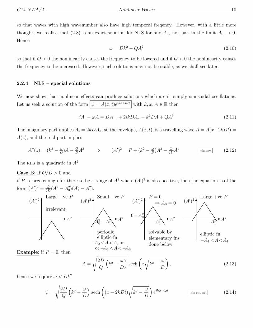
The rhs is a quadratic in A2.
Case B: If Q/D > 0 and
if P is large enough for there to be a range of A2 where (A′)2 is also positive, then the equation is of the
form (A′)2 = Q2D
(A2 − A20)(A
21 − A2).
Large −ve P
-
6
A2
(A′)2
JJ
JJJ
ªª
ªªª
irrelevant
Small −ve P
-
6
A2
(A′)2
JJ
JJJ
ªª
ªªªA2
0 A21
periodicelliptic fn
A0<A<A1 oror−A1<A<−A0
P = 0⇒ A0 = 0
-
6
A2
(A′)2
JJ
JJJ
ªª
ªªª
0=A20
A21
solvable byelementary fnsdone below
Large +ve P
-
6
A2
(A′)2J
JJ
JJ
ªª
ªªª A2
1
elliptic fn−A1<A<A1
Example: if P = 0, then
A =
√
2D
Q
(
k2 − ω
D
)
sech
(
z
√
k2 − ω
D
)
, (2.13)
hence we require ω < Dk2
ψ =
√
2D
Q
(
k2 − ω
D
)
sech
(
(x+ 2kDt)
√
k2 − ω
D
)
eikx+iωt. nls-env-sol (2.14)
G14 NWA/2 Nonlinear Waves 11
This solution is known as the bright soliton. Stability ?
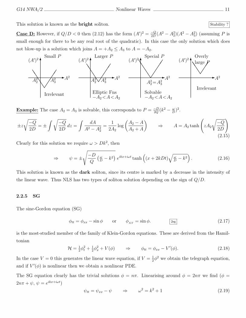
Case D: However, if Q/D < 0 then (2.12) has the form (A′)2 = −Q2D
(A2 − A22)(A
2 − A23) (assuming P is
small enough for there to be any real root of the quadratic). In this case the only solution which does
not blow-up is a solution which joins A = +A2 ≤ A3 to A = −A2.
Small P
-
6
A2
(A′)2
ªª
ªªª
JJ
JJJ
A22 A2
3
Irrelevant
Larger P
-
6
A2
(A′)2
ªª
ªªª
JJ
JJJ
A22 A2
3
Elliptic Fns−A2<A<A2
Special P
-
6
A2
(A′)2
ªª
ªªª
JJ
JJJ
A22=A2
3
Solvable−A2<A<A2
Overlylarge P
-
6
A2
(A′)2
ªª
ªª
JJ
JJ
Irrelevant
Example: The case A2 = A3 is solvable, this corresponds to P = −D2Q
(k2 − ωD)2.
±z
√
−Q
2D= ±
∫√
−Q
2Ddz =
∫
dA
A2 − A22
=1
2A2log
(
A2 − A
A2 + A
)
⇒ A = A2 tanh
(
zA2
√
−Q
2D
)
(2.15)
Clearly for this solution we require ω > Dk2, then
⇒ ψ = ±
√
−D
Q
(
ωD− k2
)
eikx+iωt tanh(
(x+ 2kDt)√
ωD− k2
)
. (2.16)
This solution is known as the dark soliton, since its centre is marked by a decrease in the intensity of
the linear wave. Thus NLS has two types of soliton solution depending on the sign of Q/D.
2.2.5 SG
The sine-Gordon equation (SG)
φtt = φxx − sinφ or φXT
= sinφ. 2sg (2.17)
is the most-studied member of the family of Klein-Gordon equations. These are derived from the Hamil-
tonian
H = 12φ2t +
12φ2x + V (φ) ⇒ φtt = φxx − V ′(φ). (2.18)
In the case V = 0 this generates the linear wave equation, if V = 12φ2 we obtain the telegraph equation,
and if V ′(φ) is nonlinear then we obtain a nonlinear PDE.
The SG equation clearly has the trivial solutions φ = nπ. Linearising around φ = 2nπ we find (φ =
2nπ + ψ, ψ = eikx+iωt)
ψtt = ψxx − ψ ⇒ ω2 = k2 + 1 (2.19)
G14 NWA/2 Nonlinear Waves 12
thus all wave numbers have real frequency. The other steady-states (φ = (2n+ 1)π + ψ) imply
ψtt = ψxx + ψ ⇒ ω2 = k2 − 1 (2.20)
so that waves with |k| < 1 have exponential growth. The steady-states φ = (2n+ 1)π are thus unstable
and those with φ = 2nπ are stable.
The SG potential V (φ) = 1− cosφ, has minima at φ = 2nπ which are sometimes referred to as ‘ground-
states’. [One problem which naturally arises is the evolution of a system which asymptotes to one ground
state as x → −∞ and another at x → +∞.]
Another commonly studied example of a Klein-Gordon equation is the ‘φ4’ model where V (φ) = −12φ2+
14φ4, which implies V ′(φ) = −φ+φ3 so that φ = ±1 are the (only) ground states. Unlike SG, this model
is not integrable.
The substitution φ = 4 tan−1 ψ in (2.17) eliminates the trig function in favour of polynomial nonlinearities1
(1 + ψ2)(ψtt − ψxx) = ψ(2ψ2t − 2ψ2
x − 1 + ψ2). (2.21)
It is possible to find separable solutions of this equation, letting ψ = X(x)T (t) we find
(
1
X2T 2+ 1
)
(
T
T− X ′′
X
)
=2 ÚT 2
T 2− 2(X ′)2
X2+ 1− 1
X2T 2, sg-reduc (2.22)
Although we cannot separate all x’s to one side and all t’s to the other, it is possible to satisfy this
equation. For example, X = eλx and T = eωt (with λ2 = 1 + ω2) [TW];
or T = cos(ωt) and X = αsech(βx) (for some α, β) [BR];
or X = cosh(λx) and T = αcsch(βt) [K-AK].
But note that since (2.22) is nonlinear, these solutions cannot be linearly combined to produce further
solutions. We shall examine each in turn.
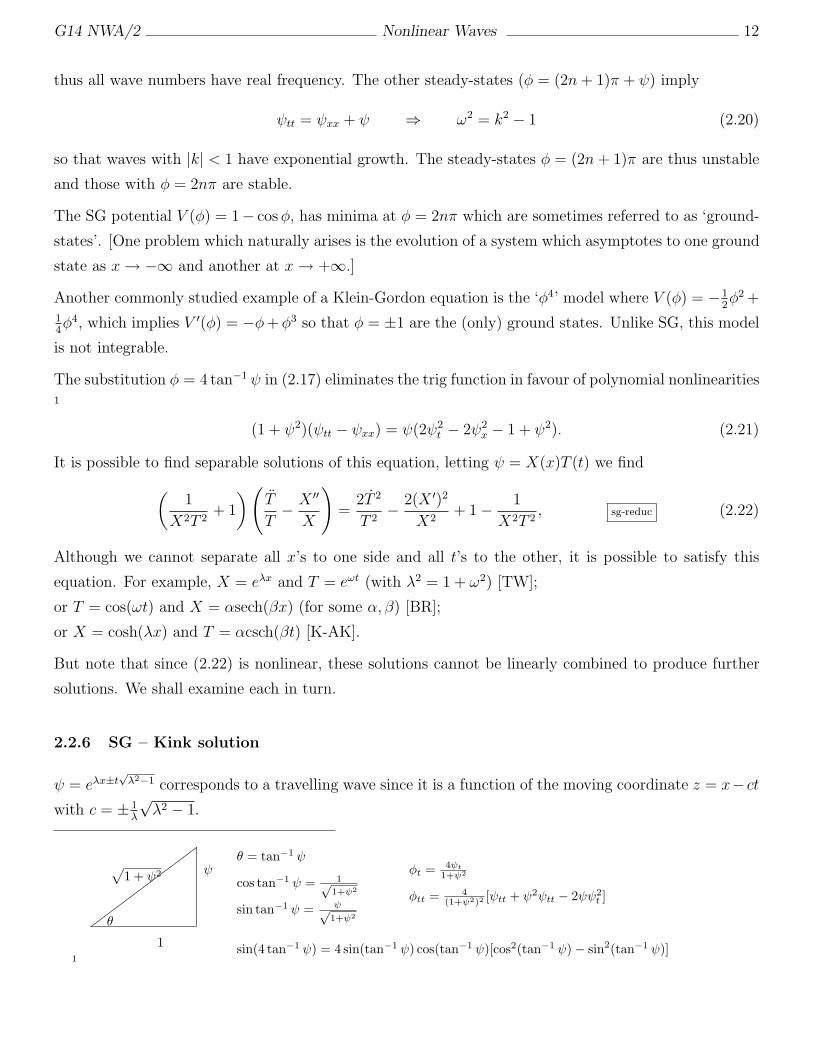
2.2.6 SG – Kink solution
ψ = eλx±t√λ2−1 corresponds to a travelling wave since it is a function of the moving coordinate z = x− ct
with c = ± 1λ
√λ2 − 1.
1
ºº
ºº
ºº
ºº
1
ψ√
1 + ψ2
θ
θ = tan−1 ψ
cos tan−1 ψ = 1√1+ψ2
sin tan−1 ψ = ψ√1+ψ2
φt =4ψt
1+ψ2
φtt =4
(1+ψ2)2 [ψtt + ψ2ψtt − 2ψψ2t ]
sin(4 tan−1 ψ) = 4 sin(tan−1 ψ) cos(tan−1 ψ)[cos2(tan−1 ψ)− sin2(tan−1 ψ)]
G14 NWA/2 Nonlinear Waves 13
Alternatively, we can seeking a travelling wave solution by assuming φ(x, t) = φ(x− ct) = φ(z), then
c2φ′′ = φ′′ − sinφ ⇒ 12(1− c2)(φ′)2 = K − cosφ. (2.23)
Assuming φ, φ′ → 0 as z → −∞ implies K = 1 and φ = 4 tan−1 eγz where γ = 1/√1− c2.
2.2.7 SG – Breather solution
ψ =√1−ω2
ωcos(ωt)sech(x
√1− ω2) yields
φ = 4 tan−1 (tan(µ) cos(t cosµ)sech(x sinµ)) (2.24)
For small values of µ this looks like a nonlinear standing wave. At larger values of µ this has the form of
a two kinks travelling in opposite directions until they reach a maximum separation at which they they
turn around and collide, passing through each other and forming a pair of negative kinks separating.
SG is invariant under the Lorentz group (cf. special relativity) x 7→ γ(x − ct), t 7→ γ(t − cx), so above
implies that
φ = 4 tan−1
(
tan(µ) cos(γ(t− cx− t0) cosµ)
cosh(γ(x− ct− x0) sinµ)
)
. (2.25)
is also a solution. We note from above that c = 1 is the maximum speed a kink can travel at. This
corresponds to the ‘speed of light’ in special relativity. Transforming to ‘light cone’ coordinates X = x+t
and T = x− t yields an alternative formulation of SG, namely
∂2φ
∂X∂T= sinφ. (2.26)
2.2.8 SG – 2-soliton solution
When X = sin(µ) cosh(x/ cosµ) and T = sinh(t tanµ) we have a kink-anti-kink collision
φ = 4 tan−1
(
sin(µ) cosh(x/ cosµ)
sinh(t tanµ)
)
(2.27)
The kinks’ positions can be described by the x-value where φ = π, giving
sinh(t tanµ) = sinµ cosh(x/ cosµ) (2.28)
As t → ∞ this asymptotes to sin(µ) exp(±x/ cosµ) = exp(t tanµ).
[Show MapleV animations here]
G14 NWA/2 Nonlinear Waves 14
2.2.9 Others
Once a couple of integrable equations had been found, the search was on, starting with generalisations
of KdV, such as the modified KdV
ut + u2ux + uxxx = 0, (2.29)
and a two-dimensional model, the Kadomtsev-Petviashvili equation (KP)
(ut + uux + uxxx)x + uyy = 0, (2.30)
and equations which allow waves to travel in both directions, such as the Boussinesq equation (Bq)
utt + (u2)xx + uxxxx = 0 (2.31)
Many systems require even symmetry, so that if u(x, t) is a solution then so is −u(x, t). Neither KdV or
Bq have this symmetry whereas mKdV, mBq (and SG) do.
Finally, there is even an example of an integrable differential–difference equation – the Toda lattice
un = (a(1− e−bun+1))− 2(a(1− e−bun)) + (a(1− e−bun−1)). (2.32)
A natural question to ask in any of these wave-bearing equations is how do waves interact ? In linear
systems we have a superposition principle whereby two solutions can be combined to produce a third by
simply adding them together, but such a procedure is not valid with nonlinear equations.
2.3 2-soliton solution - Backlund Transformation
[Recall the method of reduction of order in linear ODEs, for a second order ODE, given one solution
u1(x), can generate other by putting u2(x) = q(x)u1(x) and get a simpler problem for q(x).]
To generate more exotic solutions, it is possible to use a Backlund transformation. This typically has
the form of a pair of equations
w1,x = F (w0, w1, w0,x, w0,t;λ) BT-F (2.33)
w1,t = G(w0, w1, w0,x, w0,t;λ) BT-G (2.34)
from which we hope to generate a new solution (w1) from a known solution (w0).
2.3.1 KdV - History
In 1968 Miura showed that if v satisfies the mKdV
vt = 6v2vx − vxxx BT-mKdV (2.35)
G14 NWA/2 Nonlinear Waves 15
then u = v2 + vx solved KdV [ut = 6uux − uxxx].
By considering symmetries of mKdV and KdV we can find more ways of getting from a solution of mKdV
to a solution of KdV.
(i) KdV is invariant under x = x+ 6λt, t = t, u = u− λ:
∂∂t
= ∂∂t+ 6λ ∂
∂x∂∂x
= ∂∂x
}
ut = 6uux − uxxx
ut + 6λux = 6(u+ λ)ux − uxxx
(2.36)
so we shall work with u− λ in place of u
(ii) if v solves mKdV then so does −v, thus u = v2 − vx must also solve KdV.
Thus given a single solution v(x, t) of mKdV we have two families of solutions of KdV:
u0 = λ+ v2 + vx (2.37)
u1 = λ+ v2 − vx
Alternatively written as
u0 − u1 = 2vx (2.38)
u0 + u1 = 2λ+ 2v2
Our aim now is to eliminate v - the dependence on mKdV - so that we can go straight from one solution
of KdV to the next. Thus we shall work with w0, w1 with w0,x = u0, w1,x = u1 so that v = 12(w0 − w1),
then
w0,x + w1,x = 2λ+ 12(w1 − w0)
2 (2.39)
This has the form (2.33) and the corresponding formula (2.34) is found by requiring v = 12(w0 − w1) to
satisfy mKdV (2.35)
w1,t − w0,t = 3w21,x − 3w2
0,x − w1,xxx + w0,xxx. (2.40)
2.3.2 Example: (nothing→soliton)
To show that this method works, let us start with the trivial solution w0 = 0 and see if w1 is more
interesting. We have
w1,x = 2λ+ 12w2
1, w1,t = 3w21,x − w1,xxx (2.41)
The former is the simpler to solve, being an ODE; with λ = −k2 it gives
w1(x, t) = −2k tanh(kx+ f(t)) (2.42)
for some function f(t) to be determined.
G14 NWA/2 Nonlinear Waves 16
The former equation also implies w1,xx = w1w1,x and w1,xxx = w21w1,x + w2
1,x, so the latter equation
becomes
w1,t = 3w21,x − w2
1,x − w1,xw21 = w1,x(−4k2) ⇒ ft = −4k3. (2.43)
Thus w1 = −2k tanh(k(x− 4k2t)) and the new solution is u1 = w1,x = −4k2sech2(k(x− 4k2t)).
2.3.3 Example: (1-soliton→2-soliton)
Let us now use the method to create something new.
w2,x = 2µ+ 12(w2 − w1)
2 − w1,x (2.44)
w2,t = 3w22,x − 3w2
0,x − w2,xxx + w1,xxx + w1,t
And out of Frankenstein’s box comes forth
u=−2k21e
k1x−k31t + k22e
k2x−k32t−k0 + 2(k2 − k1)2ek1x+k2x−k31t−k32t−k0 + Aek1x+k2x−k31t−k32t−k0(k2
2ek1x−k31t + k2
1ek2x−k32t−k0)
(1 + ek1x−k31t + ek2x−k32t−k0 + Aek1x+k2x−k31t−k32t−k0)2
(2.45)
where A = (k2 − k1)2/(k2 + k1)
2, λ = −k21, µ = −k2
2.
2.3.4 Backlund Transformation for SG
Using the ‘light-cone’ formulation of SG (φXT
= sinφ) the formulae
∂θ
∂X=
∂φ
∂X+ 2λ sin(1
2(θ + φ)), (2.46)
∂θ
∂T= − ∂φ
∂T+
2
λsin(1
2(θ − φ)),
imply
θXT = φXT + λ(ΘT + φT ) cos(12(θ + φ))
= φXT + 2 sin(12(θ − φ)) cos(1
2(θ + φ)) (2.47)
θXT = −φXT +1
λ(θX − φX) cos(
12(θ − φ))
= −φXT + 2 sin(12(θ + φ)) cos(1
2(θ − φ)).
These two expressions for θXT are consistent only if φXT = sinφ, and by adding the two expressions we
find θXT = sin θ.
G14 NWA/2 Nonlinear Waves 17
2.3.5 Application of BT for SG
Using φ = 0, we use the above Backlund transformation to generate a new solution for SG, this requires
us to solve
θT = 2λ sin(12θ), θX = 2 sin(1
2θ)/λ, (2.48)
which yields the (already-known) solitary wave
θ = 4 tan−1 eλT+X/λ = 4 tan−1 ex(λ+1/λ)−t()λ−1/λ = 4 tan−1 e(x−ct)/√1−c2 (2.49)
since X = x+ t, T = x− t and λ2 = 1+c1−c
⇔ c = λ2−1λ2+1
.
2.4 Lax pairs
If we have two equations for one unknown, then in general we do not expect a solution to exist. However,
if a solution exists, then the two equations must be compatible – and there is a compatibility condition.
For example
ax+ b = 0
cx+ d = 0
}
⇔ x =−b
a=
−d
c︸ ︷︷ ︸
solution
⇔ ad− bc = 0︸ ︷︷ ︸
compatibility condition
. (2.50)
Another example: Suppose
Úx = A(t)x+B(t)
Úx = C(t)x+D(t)
}
⇔ x =D(t)−B(t)
A(t)− C(t)laxegsimp (2.51)
by equating the rhss of the two equations. However, this must actually solve the differential equation,
so substituting into Úx = Ax+B yields
(A ÚD −D ÚA) + ( ÚBC −B ÚC) + ( ÚAB − A ÚB) + ( ÚCD − C ÚD) = (A− C)(AD −BC). (2.52)
This is the compatibility condition which (A,B,C,D) must satisfy if the overdetermined linear system
(2.51) is to have a solution. Note that the compatibility condition is nonlinear even though the problem
for x is linear.
With A being a nonlinear operator not involving t-derivatives, constructing a Lax pair typically involves
rewriting the equation
ut = A(u) gen-nlop (2.53)
as
Lt = ML− LM lax (2.54)
G14 NWA/2 Nonlinear Waves 18
where L,M are linear operators in x, for example. Consider the eigenvalue problem for ψ(x, t) defined
by Lψ = λψ, then
λtψ + λψt = Ltψ + Lψt
λtψ = [ML− LM ]ψ + Lψt − λψt
λtψ = MLψ − LMψ + Lψt − λψt (2.55)
λtψ = λMψ + Lψt − LMψ − λψt
λtψ = λ(Mψ − ψt) + L(ψt −Mψ)
so if ψ evolves according to ψt = Mψ then the eigenvalue λ remains constant, so if ψ(x, 0) is an
eigenfunction then so is ψ(x, t) for all t > 0. This is a very special property of the system, and only a few
special systems (2.53) have the property of being expressible as (2.54); the quest for such decompositions
goes on.
2.4.1 Lax pair for KdV
Consider
L = − ∂2
∂x2+ u(x, t) (2.56)
then (details are not really for public consumption, but will illustrate the point)
Lψ = −ψxx + uψ
hence (Lψ)t = −ψxxt + uψt + utψ.
Note that Lψt = −ψxxt + uψt
so Ltψ = utψ ⇒ Lt = ut. (2.57)
Now to choose M : KdV has ∂xxx terms and u∂x terms, so let us try
M = βu∂
∂x+ β
∂
∂xu− α
∂3
∂x3(2.58)
then
Mψ = βuψx + βuψx + βuxψ − αψxxx
MLψ = −βuψxxx + βu2ψx + βuuxψ − βuψxxx − βuxψxx + βu2ψx + 2βuuxψ
+αψxxxxx − αuψxxx − 3αuxψxx − 3αuxxψx − αuxxxψ
LMψ = −βuψxxx − 2βuxψxx − βuxxψx − βuψxxx − 3βuxψxx − 3βuxxψx − βuxxxψ + αxxxxx
+βu2ψx + βu2ψx + βuuxψ − αuψxxx
(ML− LM)ψ = (3α− 4β)uxψxx + (3α− 4β)uxxψx + (αuxxx − βuxxx − 2βuux)ψ (2.59)
G14 NWA/2 Nonlinear Waves 19
So if we choose β = 3 and α = 4, the condition Lt = ML− LM is equivalent to ut = uxxx − 6uux.
The Lax pair enables the nonlinear problem for u to be posed as a sequence of linear problems for ψ,
which can in principle be solved and the solution can be used to determine u(x, t).
2.4.2 NLS
For NLS with Q = 2/(1− p2) and D = 1 (iut + uxx +Q|u|2u)
L = i
(
1 + p 0
0 1− p
)
∂
∂x+
(
0 u∗
u 0
)
(2.60)
A = iM = −p
(
1 0
0 1
)
∂2
∂x2+
(
|u|21+p
iu∗x
−iux−|u|21−p
)
(2.61)
where u∗ is the complex conjugate of u. The above calculation can be reworked with Lt = i(LA− AL)
and iψt = Aψ. (Exercise)
2.5 Conserved quantities
Any equation of the form∂F
∂t+
∂G
∂x= 0 cons-form (2.62)
can be thought of as a conservation law (usually neither F or G involve t-derivatives); F and G are
functions of (x, t, u, ux, uxx, uxxx, . . .). If limx→∞G = limx→−∞G then we can integrate (2.62) over all x
and find a constant of the motion,∫
F dx.
2.5.1 KdV - motivation
[Qu: Can you write KdV in the form (2.62) ?]
Ans1: F1 = u, G1 = uxx − 3u2. [Mass M =∫
u]
Ans2: F2 = u2, G2 = uuxx − 12u2x − 2u3. [Momentum P =
∫
u2]
Ans3: F3 = 2u3 + u2x, G3 = −9u4 + 6u2uxx − 12uu2
x + 2uxuxxx − u2xx. [Energy E =
∫
2u3 + u2x]
Ans4: F4 = 5u4 + 10uu2x + u2
xx [I4 =∫
5u4 + 10uu2x + u2
xx]
Ans5: F5 = 21u5 + 105u2u2x + 21uu2
xx + u2xxx
What do∫
F4 dx and∫
F5 dx correspond to ?
What is going on ?
Is there a systematic way to find Fn ?
G14 NWA/2 Nonlinear Waves 20
2.5.2 KdV-theory
Using a generalisation of the Miura transformation (see (2.35))
u = w + εvx + ε2v2 gen-miura (2.63)
the KdV equation can be written
ut−6uux+uxxx = wt+εwxt+2ε2wwt−6(w+εwx+ε2w2)(wx+εwxx+2ε2wwx)+wxxx+εwxxxx+2ε2(wwx)xx
=
(
1 + ε∂
∂x+ 2ε2w
)
(
wt − 6(w + ε2w2)wx + wxxx
)
(2.64)
So if w solves
0 = wt − 6(w + ε2w2)wx + wxxx (2.65)
then u given by (2.63) solves KdV.
Now this has the form of a conservation equation (2.62) involving the parameter ε
0 = (w)t + (wxx − 3w2 − 2ε2w3)x (2.66)
so∫
w dx is a conserved quantity.
Now we assume that w can be written as an asymptotic series in the parameter ε
w ∼∞∑
n=0
εnwn(x, t) as ε → 0, (2.67)
then each of∫
wn dx must be a conserved quantity. Substituting this expansion into (2.63) we find
u ∼∞∑
n=0
εnwn +∞∑
n=0
εn+1wn,xε2
(
∞∑
n=0
εnwn
)2
∼ w0 + εw1 + εw0,x + ε2w2 + ε2w1,x + ε2w20 + . . . (2.68)
Thus we have w0 = u as the first conserved quantity, w1 = −ux as the second (though this is trivial
since∫
w1 =∫
−ux = u(−∞, t)− u(+∞, t) and so is guaranteed simply by the BCs and tells us nothing
about the system itself); the third is w2 = −w1,x −w20 = uxx − u2 which is commonly interpreted as the
energy.
All odd n’s produce trivial conserved quantities, only the wn’s corresponding to even n’s giving useful
information.
2.5.3 NLS
For NLS, the first few conserved quantities are∫
|ψ|2 dx,∫
i(qq∗x − q∗qx) dx,
∫
|qx|2 − |q|4 dx, (2.69)
which correspond to norm, momentum and energy.
G14 NWA/2 Nonlinear Waves 21
3 Methods – for nonintegrable systems
3.1 Easy example (NLS)
We would like to check whether small additional terms in the NLS significantly affect the nature of
solutions. Suppose we perturb the NLS equation by the addition of a term
iψt = Dψxx +Q|ψ|2ψ + εψ 3p1 (3.1)
then how does ε 6= 0 influence the solution ψ(x, t) ?
Answer: (Trick): ψ(x, t) = h(t)θ(x, t)
(If |h| > 1 then solution is amplified, if |h| < 1 then solution is diminished, etc.)
If we assume |h|2 = 1 then we find
ihtθ
h+ iθt = Dθxx +Q|θ|2θ + εθ (3.2)
so that θ satisfies an unperturbed NLS equation if h = e−iεt. So the temporal frequency of the solution
is altered, while the solution’s amplitude is left unchanged. So (3.1) is integrable.
3.2 Harder example – collective variables (NLS)
Suppose we perturb the NLS equation by the addition of the term −iεψ:
iψt −Dψxx −Q|ψ|2ψ = −iεψ =: εR NLS-gen-hardeg (3.3)
then what happens to the solution ψ(x, t) ?
If ε is small we still expect the solution to have the form of a solution to NLS. For example, if D,Q are
such that there is an envelope solution we expect the perturbation to maintain this, although it may
slightly alter its height, width, speed of travel etc. [Balancing temporal derivative with perturbation
yields ψt = −εψ, so we might expect some sort of decay.]
The method of collective variables enables one to study the solution in terms of these characteristic
parameters; if ε = 0 then these quantities are all constant, but with ε 6= 0, we allow them to vary slowly.
Take the solution of the unpertubed problem (ε = 0) as
ψ = A sech(A(x− p(t)))eik(x−p(t))+iσ(t). nls-ass-sol (3.4)
By comparison with (2.14) we know that in the case D/Q > 0, (3.3) has a solution of the form p(t) = −2kt
and σ = (ω − 2k2)t. We now generate this solution by another technique.
G14 NWA/2 Nonlinear Waves 22
Assuming (3.4) is a solution for some p(t), k(t), σ(t), A(t) we determine these from
L = 12i(ψ∗ψt − ψ∗
tψ)− |ψx|2 + |ψ|4, (3.5)
hence the Lagrangian integral is
L =
∫
L dx = 23A3 − 2Ak2 + 2Ak Úp− 2A Úσ. (3.6)
In the unperturbed problem, the Euler-Lagrange equations reduce to
ddt
∂L∂ Úσ
− ∂L∂σ
= 0 ⇒ ddt(2A) = 0 ⇒ ÚA = 0 ⇒ A = A0
ddt
∂L∂ Úp
− ∂L∂p
= 0 ⇒ ddt(−2Ak) = 0 ⇒ Úk = 0 ⇒ k = k0
∂L∂k
= 0 ⇒ −4Ak + 2A Úp = 0 ⇒ Úp = 2k0 ⇒ p = 2k0t∂L∂A
= 0 ⇒ 2A2 − 2k2 + 2k Úp− 2 Úσ = 0 ⇒ Úσ =A2+k2 ⇒ σ = (A20+k2
0)t.
(3.7)
confirming what has already been obtained.
In the presence of perturbations (ε 6= 0) however, the Euler-Lagrange equations are modified.
Let y denote any one of our ‘collective coordinates’ (A, k, σ, p), then
∂L
∂y=
∫
{
∂L∂ψ
∂ψ
∂y+
∂L∂ψt
∂ψt
∂y+
∂L∂ψx
∂ ∂∂xψ
∂y
}
+
{
∂L∂ψ∗
∂ψ∗
∂y+
∂L∂ψ∗
t
∂ψ∗t
∂y+
∂L∂ψ∗
x
∂ψ∗x
∂y
}
dx
=
∫ {
∂L∂ψ
∂ψ
∂y+
∂L∂ψt
∂ψt
∂y− ∂
∂x
(
∂L∂ψx
)
∂ψ
∂y
}
+ {c.c.} dx (3.8)
and
d
dt
(
∂L
∂ Úy
)
=
∫
∂
∂t
(
∂L∂ψt
∂ψt
∂ Úy
)
+∂
∂t
(
∂L∂ψ∗
t
∂ψ∗t
∂ Úy
)
dx
=
∫
∂
∂t
(
∂L∂ψt
∂ψ
∂y
)
+ c.c. dx (3.9)
=
∫ {
∂
∂t
(
∂L∂ψt
)
∂ψ
∂y+
∂L∂ψt
∂ψt
∂y
}
+ c.c. dx
so∂L
∂y− d
dt
∂L
∂ Úy=
∫ {
∂L∂ψ
− ∂
∂t
∂L∂ψt
− ∂
∂x
∂L∂ψx
}
∂ψ
∂y+ c.c. dx EL-mod (3.10)
Now, the term in curly braces is the c.c. of the equation of motion (3.3)
{} = −iψ∗t + ψ∗
xx + 2|ψ|2ψ∗ = εR∗ = iεψ∗ in our case (3.11)
so that (3.10) becomes∂L
∂y− d
dt
∂L
∂ Úy= ε
∫
R∂ψ∗
∂ydx+ c.c. =: εRy. (3.12)
G14 NWA/2 Nonlinear Waves 23
Using (3.4) we find
∂ψ
∂k= ψi(x−p),
∂ψ
∂σ= iψ,
∂ψ
∂A= ψ[
1
A−(x−p) tanh(A(x−p))], ∂ψ
∂p= ψ[A tanh(A(x−p))−ik],
(3.13)
and thus the integrals are
Rk = i
∫
ψ∗ψk − ψψ∗k dx = i
∫
|ψ|22i(x− p) dx = 0
Rσ = i
∫
ψ∗ψσ − ψψ∗σ dx = i
∫
−2|ψ|2 dx = −4A (3.14)
RA = i
∫
ψ∗ψA − ψψ∗A dx = i
∫
|ψ|2[ 1A− (x− p) tanh()− 1
A+ (x− p) tanh()] dx = 0
Rp = i
∫
ψ∗ψk − ψψ∗k dx = i
∫
|ψ|2[A tanh()− ik − A tanh()− ik] dx = 4kA
Thus we find
∂L∂σ
− ddt
∂L∂ Úσ
= εRσ ⇒ 2 ÚA = −4εA ⇒ ÚA = −2εA ⇒ A = A0e−2εt
∂L∂p
− ddt
∂L∂ Úp
= εRp ⇒ −2 ddt(Ak) = 4εAk ⇒ Úk = 0 ⇒ k = k0
∂L∂k
= εRk ⇒ −4Ak + 2A Úp = 0 ⇒ Úp = 2k ⇒ p = 2k0t∂L∂A
= εRA ⇒ 2A2 − 2k2 + 2k Úp− 2 Úσ = 0 ⇒ Úσ =A2+k2 ⇒ σ =k20t+A
20(1−e−4εt)/4ε
(3.15)
Hence
ψ(x, t) ' A0e−2εteik0(x+2k0t)+ik20t+iA2
0(1−exp(−4εt))/4εsech((x+2k0t)A0e−2εt). (3.16)
Thus amplitude decays exponentially, and the wave spreads out, its width growing exponentially, but
surprisingly, its speed is not reduced nor is its temporal frequency altered.
3.3 Forcing and damping in SG
In the theory of Long Josephson junctions derived later, we obtain the damped and drived sine-Gordon
equation
φtt = φxx − Γ2 sinφ− I − αφt (3.17)
In order to convert this to the more familiar SG-form seen earlier we rescale the independent variables,
ξ = Γx, τ = Γt to arrive at
φττ = φξξ − sinφ− I
Γ2− α
Γφτ . 3-sg-ctm2 (3.18)
3.3.1 Ground States
We can easily see that the ‘ground’ states which any kink connects are given by solutions of
sin φ = − I
Γ2, (3.19)
G14 NWA/2 Nonlinear Waves 24
which has real solutions provided |I| < Γ2. We will define these solutions by φ± = − sin−1(I/Γ2) + 2nπ.
(The ‘+’ subscript refers to the value of φ in the limit z → +∞, and ‘–’ to the z → −∞ limit.) If
|I| ≥ Γ2 then there are no solutions. Hence we have a single kink solution if |I| < Γ2.
3.3.2 Kink solution
The terms in this equation can be placed in 3 categories:
(i) those which appear in SG
(ii) a forcing term I which adds energy to the system
(iii) a damping term involving α. Equation (3.18) with α = I = 0 is a Hamiltonian (and Lagrangian)
system, with
H =
∫
H dx =
∫
12φ2τ +
12φ2ξ + (1− cosφ) dξ
L =
∫
L dx =
∫
12φ2τ − 1
2φ2ξ − (1− cosφ) dξ. (3.20)
We seek an approximate solution to equation (3.18) with I/Γ2, α/Γ small by assuming that the forcing
and damping do not change the shape of the wave at leading order, so that we still have the solution
φ(z) = 4 tan−1(exp(γ(ξ − cτ))), 43aphi (3.21)
for some c and with γ = 1/√1− c2. For this solution
H =8√
1− c2. H-ljj (3.22)
Intuituively, we expect the forcing current (I) to add energy to the solution, increasing the speed of
the kink, and the damping term (α) to remove energy, slowing it down. These two effects may find an
equilibrium point where they balance each other out, and the kink has an equilibrium speed.
In many examples the Hamiltonian, H, is a measure of energy, and so we calculate the change of energy
in the full system (α, I 6= 0) by calculating dHdτ
using the full equation of motion. This gives
dH
dτ= −
∫
I
Γ2φτ +
α
Γφ2τ dξ (3.23)
As already noted energy can be added to the system by the forcing term, and removed via the damping
terms, however in the long run the system will settle down to an equilibrium (i.e. state of constant
energy). The speed of the kink in this equilibrium will depend upon the parameters α, I,Γ and can be
calculated by setting dHdτ
= 0. Substituting our assumed form (3.21) into (3.23) we find
2πIc
Γ2+
8αγc2
Γ= 0 ⇒ ceq =
πI√π2I2 + 16α2Γ2
. 43cdef1 (3.24)
G14 NWA/2 Nonlinear Waves 25
3.3.3 Behaviour at intermediate times
How does kink get to speed ceq ?
The kink speeds up (if c < ceq) or slows down (if c > ceq) towards the correct speed. We can find how, by
letting c depend on t using and then using (3.22) and (3.23). If c depends on t then dH/dτ from (3.22)
will not be zero, ratherdH
dτ=
8c
(1− c2)3/2dc
dτ, (3.25)
and (3.23) impliesdH
dτ=
2πIc
Γ2− 8αγc2
Γ, (3.26)
so thatdc
dτ=
πI(1− c2)3/2
4Γ2− αc(1− c2)
Γ(3.27)
3.3.4 Summary – Power Balancing
Many equations of the form φtt − E(φ) = 0 are force balances derived in some manner from Newton’s
third law. In the absence of friction and forcing they may have wave-type solutions which can travel at
an arbitrary speed (in our example any −1 < c < 1).
The presence of small forcing and damping terms can then pick out one particular wave speed at which
the energy input by forcing exactly balances the energy lost to damping. This can be found by power
balancing.
If we write the perturbed system by φtt − E(φ) = εF (φ) + εD(φ), then since power = force × velocity,
we find the equilibrium speed by requiring∫
F (φ)φt +D(φ)φtdx = 0. DERIVE
3.4 Nonsymmetric Klein-Gordon breather
Since φtt = φxx − sinφ has a breather solution, we might expect φtt = φxx − φ + 16φ3 also to have a
breather solution in the small amplitude limit; (exercise); but what about
φtt = φxx − φ+ αφ2 + βφ3nskg (3.28)
This system has Hamiltonian density
H = 12φ2t +
12φ2x +
12φ2 − 1
3αφ3 − 1
4βφ4 (3.29)
(i) dispersion relation: ω2 = k2 + 1, has minimum at k = 0 where ω = 1, so basic wave is φ = eit.
(ii) asymptotic expansion, let us look for a slowly varying envelope solution for this wave, instead of
G14 NWA/2 Nonlinear Waves 26
having a constant amplitude. We also need to account for small changes in frequency - i.e. small changes
over longer times, thus we use multiple timescales.
Introduce new timescale τ = ε2t, so ∂∂t
7→ ∂∂t+ ε2 ∂
∂τ
large space scale y = εx, so that ∂∂x
= ε ∂∂y
φ = εeitF (y, τ) + [ε2e2itG(y, τ) + ε2H(y, τ)] + [ε3e3itJ(y, τ) + ε3eitK(y, τ)] + c.c.+O(ε4) 4p-ans
(3.30)
Preliminaries:
φtt = −εeitF + 2iε3eitFτ + ε5eitFττ + ε6Hττ − 4ε2e2itG+ 4iε4e2itGτ + ε6e2itGττ
−9ε3e3itJ − ε3eitK + c.c.+ h.o.t.
φxx = ε2φyy = ε3eitFyy + c.c.+ h.o.t. (3.31)
φ2 = (ε2e2itF 2 + ε2|F |2) + (2ε3e3itFG+ 2ε3eitFH + 2ε3eitFH + 2ε3eitFG) + c.c.+O(ε4)
φ3 = (ε3e3itF 3 + 3ε3eit|F |2F ) + c.c.+ h.o.t.
where h.o.t. refers to higher order terms.
Final subs of (3.30) and all its condequences into (3.28)
−εeitF + 2iε3eitFτ − 4ε2e2itG− 9ε3e3itJ − ε3eitK = ε3eitFyy − εeitF − ε2H − ε2e2itG− ε3e3itJ
−ε3eitK + αε2e2itF 2 + αε2|F |2 + 2αε3eitFH +
+2αε3eitFH + 2αε3eitFG+ 2αε3e3itFG+
+βε3e3itF 3 + 3βε3eit|F |2F (3.32)
Now equate terms of equal order in ε and equal frequency, i.e. equal powers of eit
O(εeit) : −F = −F
O(ε2e0it) : 0 = −H + α|F |2
O(ε2e2it) : −4G = −G+ αF 2
O(ε3eit) : −K + 2iFτ = Fyy −K + 3β|F |2F + 2α(FH + FH + FG)
O(ε3e3it) : −9J = −J + βF 3 + 2αFG
(3.33)
Thus H = α|F |2, G = −13αF 2, and the last equation becomes
2iFτ = Fyy + (103α2 + 3β)|F |2F, (3.34)
which is the NLS again. Thus we can quote the solution
F =
√6 γ
√
9β + 10α2e−iγ2τ/2sech(γy) (3.35)
G14 NWA/2 Nonlinear Waves 27
which gives the leading-order result
φ(x, t) =2√6 γε
√
9β + 10α2sech(γεx) cos((1− 1
2ε2γ2)t). (3.36)
However, if 9β + 10α2 < 0 this solution is not valid, and instead we find
F = γ
√
−6
9β + 10α2eiγ
2τ tanh(γy) (3.37)
and
φ(x, t) = 2εγ
√
−6
9β + 10α2tanh(γεx) cos((1 + ε2γ2)t) (3.38)
Note that in both of these solutions γ, ε do not appear independently, but only as the product γε, thus
we have a one-parameter family of solutions, parameterised by γ = γε.
3.5 Numerical Solution of Equations
– not formally part of notes.
Standard finite difference methods for PDEs are applicable to integrable and nonlinear wave equations;
one should be aware the upwind condition in hyperbolic systems. Some numerical schemes preserve the
conserved quantities more accurately than others. For example the leap-frog scheme
un+1j − 2un
j + un−1j
(∆t)2=
unj+1 − 2un
j + unj−1
(∆x)2− F (1
2(un
j−1 + unj+1)), (3.39)
where unj = u(j∆x, n∆t) is generally more accurate for Klein-Gordon equations (utt = uxx − F (u)) than
other numerical schemes of a similar order.
Exact conservation laws provide a good check on the accuracy of the final solution.
Example
For solving KdV in 1965, Zabusky & Kruskal used the leapfrog scheme
un+1j − un−1
j
2∆t=
(
unj−1 + un
j + unj+1
3
)(
unj+1 − un
j−1
∆x
)
+uj+2 − 2uj+1 + 2uj−1 − uj−2
(∆x)3(3.40)
Note the use of central differences which improve accuracy, and the use of 13(un
j−1 + unj + un
j+1) instead
of unj ; the reason for this is to make the conservation of energy
∫
u2 more accurate. One can show that∑
j(un+1j )2 −
∑
j(un−1j )2 = O((∆t)3). (Ex)
G14 NWA/2 Nonlinear Waves 28
4 Applications
4.1 Electrical Transmission Lines
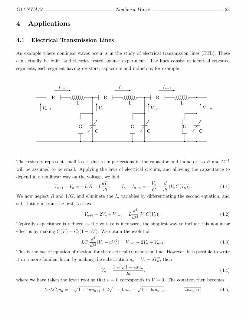
An example where nonlinear waves occur is in the study of electrical transmission lines (ETL). These
can actually be built, and theories tested against experiment. The lines consist of identical repeated
segments, each segment having resistors, capacitors and inductors; for example
-In−1 -In -In+1
6Vn−16Vn
6Vn+16Vn+2
R R R¦ ¥§¦ ¤¥§¦ ¤¥§¦ ¤¥§¦ ¤¥¦ ¥L
¦ ¥§¦ ¤¥§¦ ¤¥§¦ ¤¥§¦ ¤¥¦ ¥L
¦ ¥§¦ ¤¥§¦ ¤¥§¦ ¤¥§¦ ¤¥¦ ¥L
³³
³³7
C ³³
³³7
C ³³
³³7
CG G G
r
r
r
r
r
r
r
r
r
r
r
r
The resistors represent small losses due to imperfections in the capacitor and inductor, so R and G−1
will be assumed to be small. Applying the laws of electrical circuits, and allowing the capacitance to
depend in a nonlinear way on the voltage, we find
Vn+1 − Vn = −InR− LdIndt
, In − In−n = −Vn
G− d
dt(VnC(Vn)) . (4.1)
We now neglect R and 1/G, and eliminate the In variables by differentiating the second equation, and
subtituting in from the first, to leave
Vn+1 − 2Vn + Vn−1 = Ld2
dt2[VnC(Vn)] . (4.2)
Typically capacitance is reduced as the voltage is increased, the simplest way to include this nonlinear
effect is by making C(V ) = C0(1− aV ). We obtain the evolution
LC0d2
dt2(Vn − aV 2
n ) = Vn+1 − 2Vn + Vn−1. (4.3)
This is the basic ‘equation of motion’ for the electrical transmission line. However, it is possible to write
it in a more familiar form, by making the substitution un = Vn − aV 2n , then
Vn =1−
√1− 4aun
2a, (4.4)
where we have taken the lower root so that u = 0 corresponds to V = 0. The equation then becomes
2aLC0un = −√
1− 4aun+1 + 2√1− 4aun −
√
1− 4aun−1. etl-eqmot (4.5)

G14 NWA/2 Nonlinear Waves 29
4.1.1 Aside
This system is Hamiltonian, with forces W ′(u) = [1 −√(1 − 4au)]/2a, and since W ′′(0) > 0 the zero
solution is stable (dispersion relation gives real frequencies), we have a potential energy
W (u) =(1− 4au)3/2
12a2+
u
2a− 1
12a2, (4.6)
whence a Hamiltonian structure is obtained
H =∑
n
12s2n +W (rn+1 − rn). (4.7)
Here un = rn+1 − rn, sn = Úrn and (rn, sn) are the canonical Hamiltonian variables.
From numerical simulations we see that any disturbance in the ETL breaks down if its amplitude becomes
too large. From the equation of motion we can see this too: if u > 1/4a then we have strayed into a
region where W (u) is not well-defined, corresponding to an upper limit for V of 1/2a. Numerically
determined wave profiles, are seen to develop a singularity as the amplitude reaches this limit, cf waves
breaking on a beach.
4.1.2 Onto KdV
Let us analyse small amplitude deviations from u = 0 in this system. expanding (4.5) for small u we find
2aLC0un = 2aun+1 + 2a2u2n+1 − 4aun − 4a2u2
n + 2aun−1 + 2a2u2n−1 etl-eqmot2 (4.8)
Our spatial variable n is currently discrete, in order to convert (4.8) into something more familiar we
replace n by a continuous variable, x and expand the second central difference into spatial derivatives,
LC0utt = uxx +112uxxxx + a(u2)xx +
112a(u2)xxxx. etl-ctm1 (4.9)
This will only be valid if the waves we are seeking are slowly varying in space, otherwise u(x+1)−u(x) 6≈∂u/∂x. So we shall restrict ourselves to analysing slowly varying waves.
(4.9) has dispersion relation LC0ω2 = k2 − 1
12k4, so that slowly varying waves travel with speed ω/k ≈
(1− 124k2)/
√LC0 ≈ 1/
√LC0.
So let us look for waves which travel at about this speed, using the slow variation in u as a function of
x, we introduce a small parameter ε ¼ 1 so that (1/u)∂u∂x
∼ ε, then x needs to alter by 1/ε to alter u by
an O(1) amount.
We transform to a coordinate frame which moves at speed v, via y = ε(x− vt), with v = 1/√LC0
and study evolution on an exceedingly long timescale, τ = ε3t
G14 NWA/2 Nonlinear Waves 30
and look at small amplitude waves u = ε2ψ then
∂
∂x=
/
0.∂
∂τ
/
+ ε∂
∂y,
∂
∂t= ε3
∂
∂τ− εv
∂
∂y(4.10)
implies (4.9) becomes
LC0ε8ψττ
︸ ︷︷ ︸
h.o.t.−ignored
−2ε6vLC0ψτy + ε4v2LC0ψyy︸ ︷︷ ︸
cancels
= ε4ψyy︸ ︷︷ ︸
cancels
+ 112ε6ψyyyy + aε6(ψ2)yy +
112aε8(ψ2)yyyy
︸ ︷︷ ︸
h.o.t.−ignored
(4.11)
noting that LC0v2 = 1, we find the O(ε4) terms cancel leaving O(ε6) terms as leading order, all of which
involve a y-derivative. Thus integrating once w.r.t y we find
−2√
LC0 ψτ = 112ψyyy + 2a(ψψy) (4.12)
Simple linear rescalings of τ, yψ can remove all these constants to leave the famous KdV equation.
ψ = 24aψ
y = −y
τ = τ/24√LC0
⇒ ψτ = ψyyy + ψ ψy. (4.13)
4.1.3 Regularising long wave equations
Continuum approximations are also known as long-wave equations, since they are designed to faithfully
approximate the long wave (small wavenumber) behaviour of a more complicated system. Unfortunately
they can be ill-posed; it has already been noted that (4.8) is ill-posed in that its dispersion relation
predicts complex ω’s for large k.
We shall now use Fourier transforms to show how the above argument may be improved, through the
derivation of well-posed PDEs at intermediate stages to yield more accurate final approximations to the
shape of solitary waves.
We rewrite (4.8) as
utt(n, t) = un = W ′(u(n+ 1, t))− 2W ′(u(n, t)) +W ′(u(n− 1, t)), (4.14)
which we shall think of as an operator equation
utt = D2W ′(u(t)) where D2 = δ2n = exp(∂n)− 2 + exp(−∂n) (4.15)
since
f(n+ 1) = f(n) + 1f ′(n) + 1212f ′′(n) + 1
613f ′′′(n) + . . . (4.16)
= [1 + ∂n +12∂2n +
16∂3 + . . .]f(n). (4.17)
G14 NWA/2 Nonlinear Waves 31
We now take Fourier transforms in n,
defining u =∫∞n=−∞ u(n, t)eikndn and W ′(u) =
∫
W ′(u(n, t))eikndn so that
W ′(u(n+1, t)) =
∫
W ′(u(n+ 1, t)eikndn =
∫
W ′(u(m, t)eikm−ikdm = e−ik W ′(u), (4.18)
then
−utt = −(eik − 2 + e−ik) W ′(u) = 4 sin2(12k) W ′(u). (4.19)
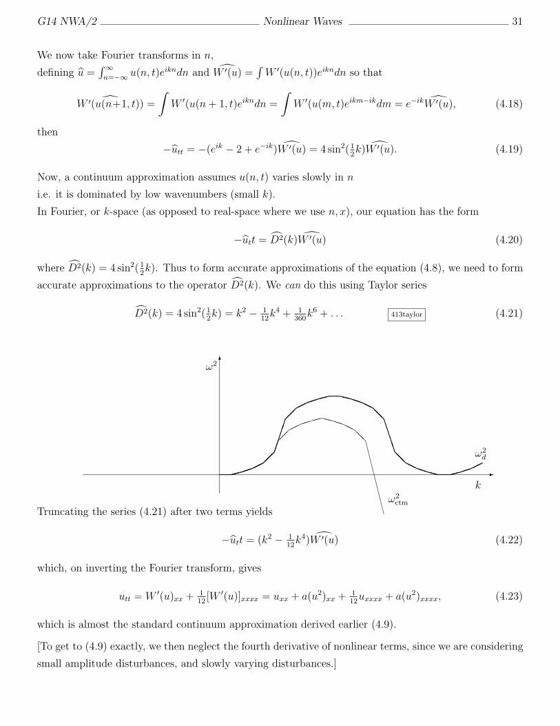
Now, a continuum approximation assumes u(n, t) varies slowly in n
i.e. it is dominated by low wavenumbers (small k).
In Fourier, or k-space (as opposed to real-space where we use n, x), our equation has the form
−utt = D2(k) W ′(u) (4.20)
where D2(k) = 4 sin2(12k). Thus to form accurate approximations of the equation (4.8), we need to form
accurate approximations to the operator D2(k). We can do this using Taylor series
D2(k) = 4 sin2(12k) = k2 − 1
12k4 + 1
360k6 + . . . 413taylor (4.21)
-
6
k
ω2
¸ °°¨ ¢¢¢¢
¨ °°¸ XXPPHH@@
BBBB@@HHPPXX ¸ °°¨
ω2d
¸ °°¨
¢¢
¨°°¸ XXPPHH
@@CCCCCCCCω2ctm
Truncating the series (4.21) after two terms yields
−utt = (k2 − 112k4) W ′(u) (4.22)
which, on inverting the Fourier transform, gives
utt = W ′(u)xx +112[W ′(u)]xxxx = uxx + a(u2)xx +
112uxxxx + a(u2)xxxx, (4.23)
which is almost the standard continuum approximation derived earlier (4.9).
[To get to (4.9) exactly, we then neglect the fourth derivative of nonlinear terms, since we are considering
small amplitude disturbances, and slowly varying disturbances.]
G14 NWA/2 Nonlinear Waves 32
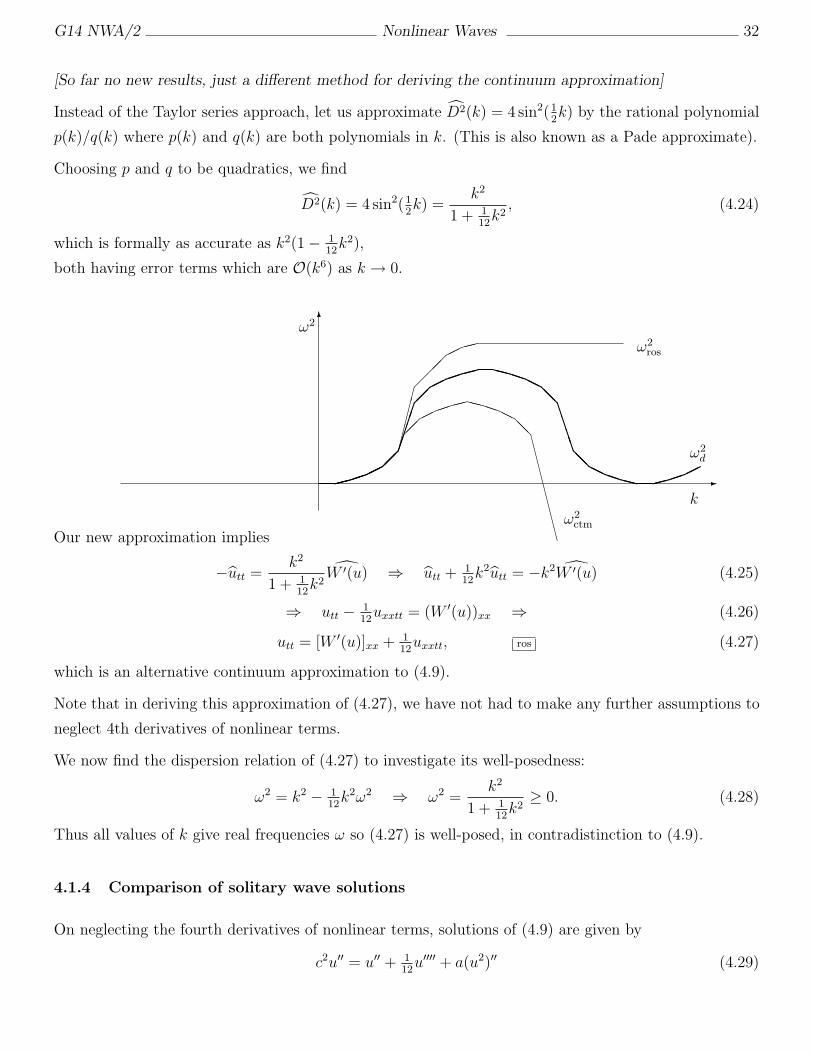
[So far no new results, just a different method for deriving the continuum approximation]
Instead of the Taylor series approach, let us approximate D2(k) = 4 sin2(12k) by the rational polynomial
p(k)/q(k) where p(k) and q(k) are both polynomials in k. (This is also known as a Pade approximate).
Choosing p and q to be quadratics, we find
D2(k) = 4 sin2(12k) =
k2
1 + 112k2
, (4.24)
which is formally as accurate as k2(1− 112k2),
both having error terms which are O(k6) as k → 0.
-
6
k
ω2
¸ °°¨ ¢¢¢¢
¨ °°¸ XXPPHH@@
BBBB@@HHPPXX ¸ °°¨
ω2d
¸ °°¨
£££££
¨
¸ ω2ros
¸ °°¨
¢¢
¨°°¸ XXPPHH
@@CCCCCCCCω2ctm
Our new approximation implies
−utt =k2
1 + 112k2
W ′(u) ⇒ utt +112k2utt = −k2 W ′(u) (4.25)
⇒ utt − 112uxxtt = (W ′(u))xx ⇒ (4.26)
utt = [W ′(u)]xx +112uxxtt, ros (4.27)
which is an alternative continuum approximation to (4.9).
Note that in deriving this approximation of (4.27), we have not had to make any further assumptions to
neglect 4th derivatives of nonlinear terms.
We now find the dispersion relation of (4.27) to investigate its well-posedness:
ω2 = k2 − 112k2ω2 ⇒ ω2 =
k2
1 + 112k2
≥ 0. (4.28)
Thus all values of k give real frequencies ω so (4.27) is well-posed, in contradistinction to (4.9).
4.1.4 Comparison of solitary wave solutions
On neglecting the fourth derivatives of nonlinear terms, solutions of (4.9) are given by
c2u′′ = u′′ + 112u′′′′ + a(u2)′′ (4.29)
G14 NWA/2 Nonlinear Waves 33
which implies
u =3
2a(c2−1) sech2
(
(x− ct)√
3(c2 − 1))
, 414ctm (4.30)
whereas solutions of (4.27) are given by
c2u′′ = u′′ + a(u2)′′ + 112c2u′′′′ (4.31)
which implies
u =3
2a(c2−1) sech2
(
(x− ct)
√
3(c2 − 1)
c2
)
. 414ros (4.32)
Looking at the amplitudes, we see that there is no difference, as is the sech shape, but the width does
vary. In (4.30) the width → 0 as c → ∞, which is unphysical and the assumption of u(z) being a slowly
varying function fails. In (4.32) the width saturates at 1/√3 as c → ∞, which is more realistic, and the
assumption of u(z) varying slowly is valid for larger values of c than in (4.30).
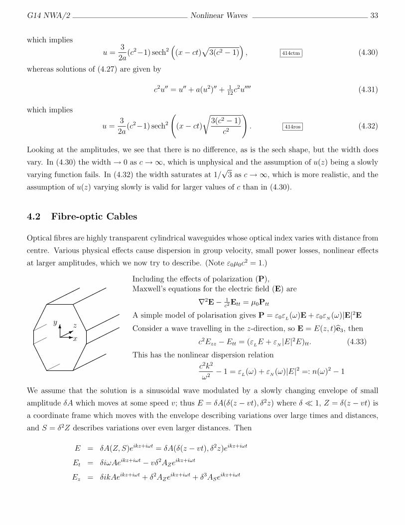
4.2 Fibre-optic Cables
Optical fibres are highly transparent cylindrical waveguides whose optical index varies with distance from
centre. Various physical effects cause dispersion in group velocity, small power losses, nonlinear effects
at larger amplitudes, which we now try to describe. (Note ε0µ0c2 = 1.)
-x6
y
¨*z
AAAA
¡¡
¡¡
¡¡¡¡
AA
AA
¨¨¨¨¨
¨¨¨¨¨
¨¨¨¨¨
¨¨¨¨¨
¨¨¨¨¨
¨¨
¨¨
¨¨
Including the effects of polarization (P),Maxwell’s equations for the electric field (E) are
∇2E − 1c2
Ett = µ0Ptt
A simple model of polarisation gives P = ε0εL(ω)E + ε0εN
(ω)|E|2EConsider a wave travelling in the z-direction, so E = E(z, t)e3, then
c2Ezz − Ett = (εLE + ε
N|E|2E)tt.
This has the nonlinear dispersion relation
c2k2
ω2− 1 = ε
L(ω) + ε
N(ω)|E|2 =: n(ω)2 − 1
(4.33)
We assume that the solution is a sinusoidal wave modulated by a slowly changing envelope of small
amplitude δA which moves at some speed v; thus E = δA(δ(z − vt), δ2z) where δ ¼ 1, Z = δ(z − vt) is
a coordinate frame which moves with the envelope describing variations over large times and distances,
and S = δ2Z describes variations over even larger distances. Then
E = δA(Z, S)eikz+iωt = δA(δ(z − vt), δ2z)eikz+iωt
Et = δiωAeikz+iωt − vδ2AZeikz+iωt
Ez = δikAeikz+iωt + δ2AZeikz+iωt + δ3ASe
ikz+iωt
G14 NWA/2 Nonlinear Waves 34
Ett = −δω2Aeikz+iωt − 2iωvδ2AZ + v2δ3AZZeikz+iωt (4.34)
Ezz = −δk2Aeikz+iωt + 2ikδ2AZeikz+iωt + δ3AZZe
ikz+iωt + 2ikδ3ASeikz+iωt +O(δ4).
(|E|2E) = δ3|A|2Aeikz+iωt
(|E|2E)t = δ3iω|A|2Aeikz+iωt +O(δ4)
(|E|2E)tt = −ω2δ3|A|2Aeikz+iωt +O(δ4)
Plugging all this into (4.33) yields
O(δ) : −c2k2 + ω2 = −εLω2
O(δ2) : c2k + ωv = −vωεL
O(δ3) : 2ikc2AS + c2AZZ + v2AZZ = −ω2εN|A|2A+ ε
Lv2AZZ
(4.35)
The first of which is the linear dispersion relation (for which it is easier to think of ω being specified and
k = k(ω) being determined by k2 = (1+εL)ω2/c2). The second fixes the speed v at which the envelope
travels, and the third is the NLS equation which determines the shape of the envelope.
2ikc2AS = AZZ(εLv2 − v2 − c2)− ε
Nω2|A|2A, v =
−c2ω
k. (4.36)
4.3 Water Waves
For those who have met Navier-Stokes equations before, we are now going to derive KdV from NS.
(Those who haven’t met NS before can have a short nap). Firstly, neglect viscosity, so we obtain the
Euler equations. For a liquid subject to gravity (acting in the negative y-direction), we have
ut + (u.∇)u = −1
%∇P − gj ns-mom (4.37)
∇.u = 0. ns-cty (4.38)
Taking the curl of (4.37) yields an equation which has vorticity w = ∇ × u = 0 as a solution. This
enables us to write u = ∇φ where φ is a velocity potential. The continuity equation (4.38) then becomes
∇2ψ = 0. The momentum conservation equation can be written as
P − P0
%= P1(t)− φt − 1
2|∇φ|2 − gy. (4.39)
The arbitrary function P1(t) can be absorbed into the velocity potential by φ = φ−∫
P1 dt;
we choose the constant P0 such that P = P0 on y = h0.
G14 NWA/2 Nonlinear Waves 35
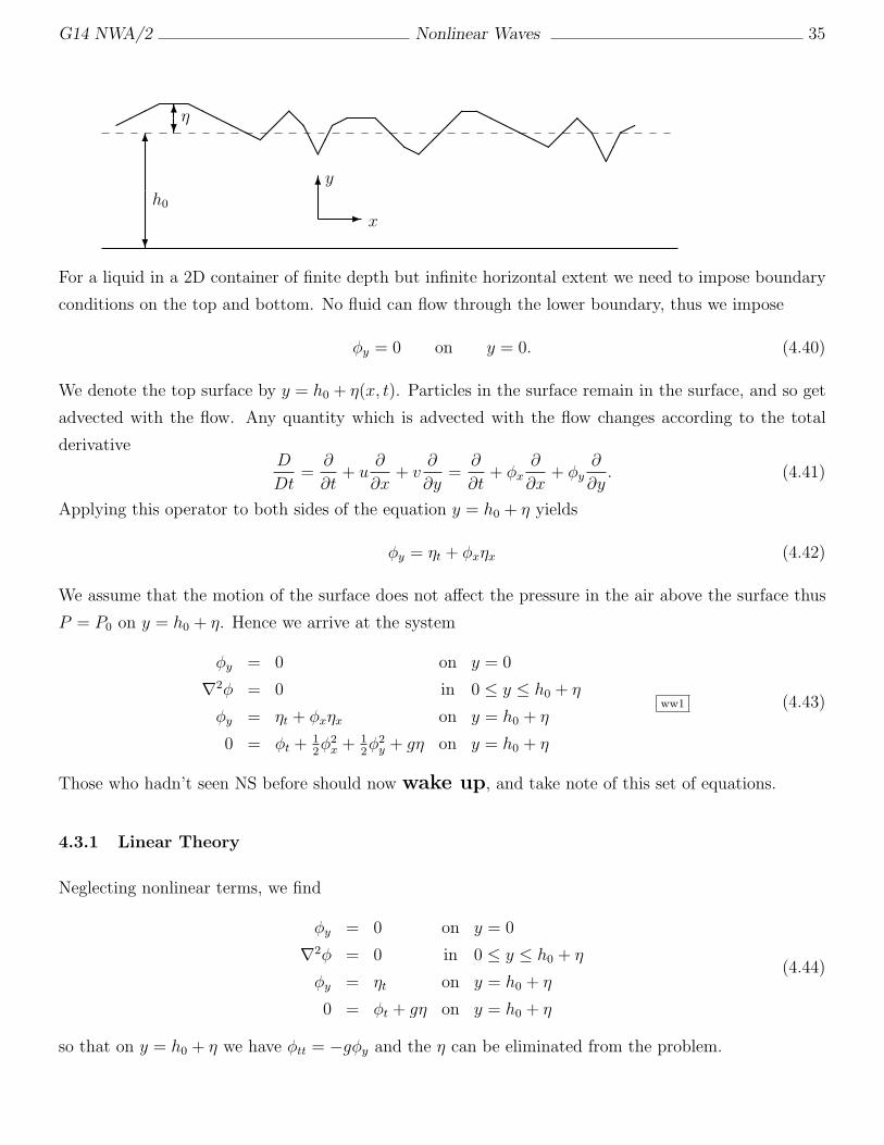
6
?
h0
?6η
-
6
x
y
¨¨¨HHHHH
@AA¡
¡¨ @
@H
HHHHH @
AA¡
¡¨
For a liquid in a 2D container of finite depth but infinite horizontal extent we need to impose boundary
conditions on the top and bottom. No fluid can flow through the lower boundary, thus we impose
φy = 0 on y = 0. (4.40)
We denote the top surface by y = h0 + η(x, t). Particles in the surface remain in the surface, and so get
advected with the flow. Any quantity which is advected with the flow changes according to the total
derivativeD
Dt=
∂
∂t+ u
∂
∂x+ v
∂
∂y=
∂
∂t+ φx
∂
∂x+ φy
∂
∂y. (4.41)
Applying this operator to both sides of the equation y = h0 + η yields
φy = ηt + φxηx (4.42)
We assume that the motion of the surface does not affect the pressure in the air above the surface thus
P = P0 on y = h0 + η. Hence we arrive at the system
φy = 0 on y = 0
∇2φ = 0 in 0 ≤ y ≤ h0 + η
φy = ηt + φxηx on y = h0 + η
0 = φt +12φ2x +
12φ2y + gη on y = h0 + η
ww1 (4.43)
Those who hadn’t seen NS before should now wake up, and take note of this set of equations.
4.3.1 Linear Theory
Neglecting nonlinear terms, we find
φy = 0 on y = 0
∇2φ = 0 in 0 ≤ y ≤ h0 + η
φy = ηt on y = h0 + η
0 = φt + gη on y = h0 + η
(4.44)
so that on y = h0 + η we have φtt = −gφy and the η can be eliminated from the problem.
G14 NWA/2 Nonlinear Waves 36
Seeking a solution in terms of linear waves travelling in the x-direction we assume
φ = A(x, y) sin(kx− ωt) (4.45)
then in 0 ≤ y ≤ h0 + η
0 =
[
∂A
∂y+
∂A
∂x− k2A
]
sin(kx− ωt) +
[
2k∂A
∂x
]
cos(kx− ωt). (4.46)
Since this equation must hold for all (x, t), both square brackets must evaluate to zero,
thus ∂A∂x
= 0 (A is independent of x∀t, i.e. A = A(y) only),
and A = A0 cosh(k(y + h0)) + A1 sinh(k(y + h0)).
Imposing the boundary condition at y = 0 yields A1 = 0.
The top boundary condition (φtt = −gφy on y = h0 + η) yields
ω2 = kg tanh(k(h0 + η)). (4.47)
Assuming h0 is small, this gives a speed of
c =ω
k=
√
g(h0 + η)− 13k2g(h0 + η)3. (4.48)
As k → 0, the wave speed c asymptotes to c0 =√gh, where h = h0 + η;
and for small k the speed can be approximated by c =√gh(1 − 1
6k2h2). Slowly varying surface distur-
bances thus propagate with this speed.
4.3.2 Nonlinear Theory
We want to analyse the long-time evolution (t → ∞) of surface waves, when the water is very shallow
(h0 → 0). Care is needed when considering a combination of limits. First we shall rescale (non-
dimensionalise), looking for waves which travel at the speed c0
y = h0Y, η = εh0H, φ = h0
√
εgh0Φ, t =1
ε
√
h0
εgT, x− c0t =
h0√εZ. (4.49)
Note that ∂t = ε√
εg/h0 ∂T − c0√ε/h0 ∂Z .
Thus the system of equations (4.43) becomes
ΦY = 0 on Y = 0
εΦZZ + ΦY Y = 0 in 0 ≤ Y ≤ 1 + εH(X,T )
ε2HT − εHZ + ε2ΦZHZ = ΦY on Y = 1 + εH(X,T ) BCY
H + εΦT − ΦZ + 12Φ2
Y + 12εΦ2
Z = 0 on Y = 1 + εH(X,T ) BCH
(4.50)
G14 NWA/2 Nonlinear Waves 37
Note that h0 has been eliminated from these equations, thus we only need to worry about the limit ε → 0
now, (which corresponds to considering wide small amplitude distubrances &t ½ 1).
Solving the system we assume a solution for Φ(Y, Z, T ) of the form
Φ = Φ0 + εΦ1 + ε2Φ2 + . . . (4.51)
Then fit this to the DE and to the lower BC to find Φ:
O(1) : Φ0,Y Y = 0 ⇒ Φ0 = A(Z, T )Y +B(Z, T )
BC ⇒ A = 0 ⇒ Φ0 = B
O(ε) : Φ1,Y Y = −Φ0,ZZ = −BZZ ⇒ Φ1 = D(Z, T ) + Y C(Z, T )− 12Y 2BZZ
BC ⇒ C = 0 ⇒ Φ1 = D − 12Y 2BZZ
O(ε2) : Φ2,Y Y =−Φ1,ZZ = 12Y 2BZZZZ −DZZ ⇒ Φ2 = 1
24Y 4BZZZZ − 1
2Y 2DZZ + E(Z, T )Y + F (Z, T )
BC ⇒ E = 0 ⇒ Φ2 = 124Y 4BZZZZ − 1
2Y 2DZZ + F
(4.52)
Thus
Φ = B + ε(D − 12Y 2BZZ) + ε2(F − 1
2Y 2DZZ + 1
24Y 4BZZZZ) +O(ε3). (4.53)
so that ΦY = −εY BZZ + ε2(16Y 3BZZZZ −Y DZZ) and ΦZ,T = . . .; we also introduce an expansion for the
disturbance H = J + εI.
Now applying BCY to O(ε2):
−εBZZ − ε2JBZZ + 16ε2BZZZZ − ε2DZZ
︸ ︷︷ ︸
ΦY
= ε2JT︸︷︷︸
ε2HT
+ ε2JZBZ︸ ︷︷ ︸
ε2HZΦZ
−εJZ − ε2IZ︸ ︷︷ ︸
−εHZ
(4.54)
Thus at O(ε) we have BZZ = JZ and at O(ε2)
DZZ − IZ = 16BZZZZ − JBZZ − JT − JZBZ WWBCY (4.55)
Imposing BCH
0 = J + εI︸ ︷︷ ︸
H
−BZZ − ε(DZ − 12BZZZ)
︸ ︷︷ ︸
−ΦZ
+ εBT︸︷︷︸
εΦT
+ 12εB2
Z︸ ︷︷ ︸
12εΦ2
Z
+O(ε2)︸ ︷︷ ︸
12Φ2
Y
(4.56)
from the O(1) terms we find J = BZ and from those O(ε) we find
DZ − I = 12BZZZ +BT + 1
2B2
Z WWBCH (4.57)
Taking ∂Z(4.57)-(4.55) we obtain
0 = 13BZZZ +BZT + JT + JTBZZ + JZBZ +BZBZZ (4.58)
but since BZ = J this can be written
0 = 13JZZZ + 2JT + 3JJZ , (4.59)
which is the KdV equation.
G14 NWA/2 Nonlinear Waves 38
4.3.3 Intepretation of Results
The KdV equation has travelling wave solutions
J = J(Z − V T ) = 2V sech2
(√
3V
2(Z − V T )
)
, (4.60)
in which H = J + O(ε) describes the shape of the fluid’s free surface. Rewriting this in the original
η(x, t) variables
η = εh0H, Z =
√ε
h0(x− c0t), c0 =
√
gh0, T = εt
√
εg
h0, (4.61)
we find
η = 2εh0V sech2
(√
3V
2
[√ε
h0(x−c0t)− εV t
√
εg
h0
]
)
(4.62)
= 2vh0sech2
(
1
h0
√
3v
2
[
x−√
gh0 (1 + v)t]
)
, (4.63)
when one notes that only the combination v = εV ¼ 1 appears, and never ε or V alone.
4.4 Long Josephson junctions
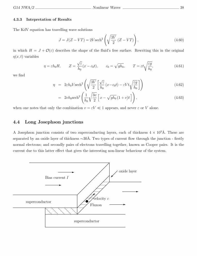
A Josephson junction consists of two superconducting layers, each of thickness 4 × 10³A. These are
separated by an oxide layer of thickness ∼30A. Two types of current flow through the junction - firstly
normal electrons; and secondly pairs of electrons travelling together, known as Cooper pairs. It is the
current due to this latter effect that gives the interesting non-linear behaviour of the system.
-
-
Bias current I
-
-
superconductor
superconductor
w ²
Fluxon
velocity c
©
oxide layer
@@
@@
@@
@@
@@
G14 NWA/2 Nonlinear Waves 39
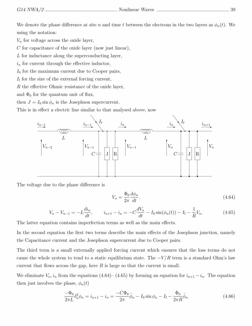
We denote the phase difference at site n and time t between the electrons in the two layers as φn(t). We
using the notation:
Vn for voltage across the oxide layer,
C for capacitance of the oxide layer (now just linear),
L for inductance along the superconducting layer,
in for current through the effective inductor,
I0 for the maximum current due to Cooper pairs,
If for the size of the external forcing current,
R the effective Ohmic resistance of the oxide layer,
and Φ0 for the quantum unit of flux,
then J = I0 sinφn is the Josephson supercurrent.
This is in effect a electric line similar to that analysed above, now
L L
-in−1 -in−1 -in -in -in+1
6Vn−2
6Vn−1
6Vn−1
6Vn
6Vn
q q q
C J R
q q qS
SwS
SqIf
r r r
C J R
r r rS
SwS
SqIf§ ¤§¦ ¤¥§ ¤§¦ ¤¥§¦ ¤¥ § ¤§¦ ¤¥§ ¤§¦ ¤¥§¦ ¤¥
The voltage due to the phase difference is
Vn =Φ0
2π
dφn
dt. (4.64)
Vn − Vn−1 = −Ldindt
, in+1 − in = −CdVn
dt− I0 sin(φn(t))− If −
1
RVn. (4.65)
The latter equation contains imperfection terms as well as the main effects.
In the second equation the first two terms describe the main effects of the Josephson junction, namely
the Capacitance current and the Josephson supercurrent due to Cooper pairs.
The third term is a small externally applied forcing current which ensures that the loss terms do not
cause the whole system to tend to a static equilibrium state. The −V/R term is a standard Ohm’s law
current that flows across the gap, here R is large so that the current is small.
We eliminate Vn, in from the equations (4.64)– (4.65) by forming an equation for in+1− in. The equation
then just involves the phase, φn(t)
−Φ0
2πLδ2nφn = in+1 − in =
−CΦ0
2πφn − I0 sinφn − If −
Φ0
2πRÚφn (4.66)
G14 NWA/2 Nonlinear Waves 40
Rescaling of time (by 1/√(LC) ), together with defining
Γ2 =2πLI0Φ0
, α =
√L
R√C, I =
2πLIfΦ0
. (4.67)
gives the driven and damped discrete sine-Gordon equation
φn = φn+1 − 2φn + φn−1 − Γ2 sinφn − I − α Úφn. (4.68)
The physical quantities of current and voltage are related to φ by i ∝ 〈φn〉, V ∝ 〈 Úφn〉.
We convert the difference terms into derivatives by replacing n with a continuous variable x and Taylor
expanding
φtt = φxx − Γ2 sinφ− I − αφt. (4.69)
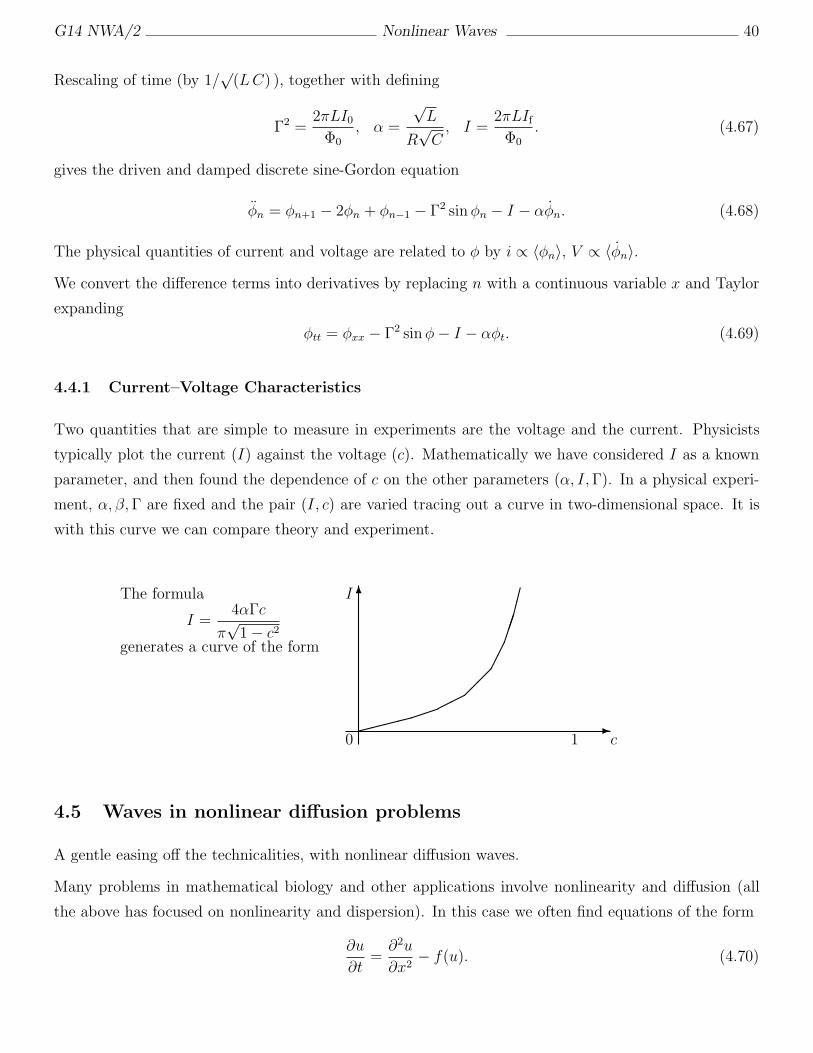
4.4.1 Current–Voltage Characteristics
Two quantities that are simple to measure in experiments are the voltage and the current. Physicists
typically plot the current (I) against the voltage (c). Mathematically we have considered I as a known
parameter, and then found the dependence of c on the other parameters (α, I,Γ). In a physical experi-
ment, α, β,Γ are fixed and the pair (I, c) are varied tracing out a curve in two-dimensional space. It is
with this curve we can compare theory and experiment.
The formula
I =4αΓc
π√1− c2
generates a curve of the form
-
6I
c0 1¸¸¸¸°°¨¨
¡¡¢¢¢££
4.5 Waves in nonlinear diffusion problems
A gentle easing off the technicalities, with nonlinear diffusion waves.
Many problems in mathematical biology and other applications involve nonlinearity and diffusion (all
the above has focused on nonlinearity and dispersion). In this case we often find equations of the form
∂u
∂t=
∂2u
∂x2− f(u). (4.70)
G14 NWA/2 Nonlinear Waves 41
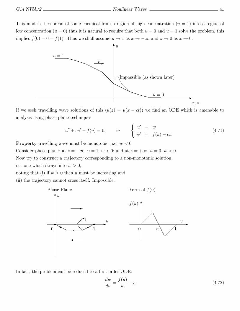
This models the spread of some chemical from a region of high concentration (u = 1) into a region of
low concentration (u = 0) thus it is natural to require that both u = 0 and u = 1 solve the problem, this
implies f(0) = 0 = f(1). Thus we shall assume u → 1 as x → −∞ and u → 0 as x → 0.
-
6
x, z
u
XXPPPHHHH@
@@HHHHPPPXX
-cu = 1
u = 0
AA@
@
Impossible (as shown later)
If we seek travelling wave solutions of this (u(z) = u(x − ct)) we find an ODE which is amenable to
analysis using phase plane techniques
u′′ + cu′ − f(u) = 0, ⇔
{
u′ = w
w′ = f(u)− cw(4.71)
Property travelling wave must be monotonic. i.e. w < 0
Consider phase plane: at z = −∞, u = 1, w < 0; and at z = +∞, u = 0, w < 0.
Now try to construct a trajectory corresponding to a non-monotonic solution,
i.e. one which strays into w > 0,
noting that (i) if w > 0 then u must be increasing and
(ii) the trajectory cannot cross itself. Impossible.
-
6
u
w
s s-
»
¨¹¨H
HHY
Phase Plane
0 1» @I
-?
Form of f(u)
-
6
u
f(u)
AAAAAA
0 1α
In fact, the problem can be reduced to a first order ODE:
dw
du=
f(u)
w− c (4.72)
G14 NWA/2 Nonlinear Waves 42
from which we can deduce information about c:
0 = [12w2]u=1
u=0 =
∫ u=1
u=0
w dw =
∫ u=1
u=0
f(u) du−∫ u=1
u=0
cw(u) du diff-ceq (4.73)
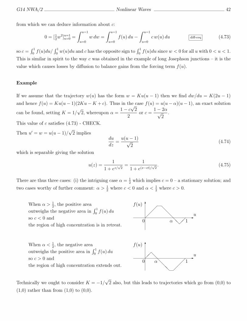
so c =∫ 1
0f(u)du/
∫ 1
0w(u)du and c has the opposite sign to
∫ 1
0f(u)du since w < 0 for all u with 0 < u < 1.
This is similar in spirit to the way c was obtained in the example of long Josephson junctions – it is the
value which causes losses by diffusion to balance gains from the forcing term f(u).
Example
If we assume that the trajectory w(u) has the form w = Ku(u − 1) then we find dw/du = K(2u − 1)
and hence f(u) = Ku(u− 1)(2Ku−K + c). Thus in the case f(u) = u(u− α)(u− 1), an exact solution
can be found, setting K = 1/√2, whereupon α =
1− c√2
2or c =
1− 2α√2
.
This value of c satisfies (4.73) - CHECK.
Then u′ = w = u(u− 1)/√2 implies
du
dz=
u(u− 1)√2
(4.74)
which is separable giving the solution
u(z) =1
1 + ez/√2=
1
1 + e(x−ct)/√2. (4.75)
There are thus three cases: (i) the intriguing case α = 12
which implies c = 0 – a stationary solution; and
two cases worthy of further comment: α > 12
where c < 0 and α < 12
where c > 0.
-
6
u
f(u)
@@
@@@ 0 1α
-
6
u
f(u)
@@
@@@
0 1α
When α > 12, the positive area
outweighs the negative area in∫ 1
0f(u) du
so c < 0 and
the region of high concentration is in retreat.
When α < 12, the negative area
outweighs the positive area in∫ 1
0f(u) du
so c > 0 and
the region of high concentration extends out.
Technically we ought to consider K = −1/√2 also, but this leads to trajectories which go from (0,0) to
(1,0) rather than from (1,0) to (0,0).
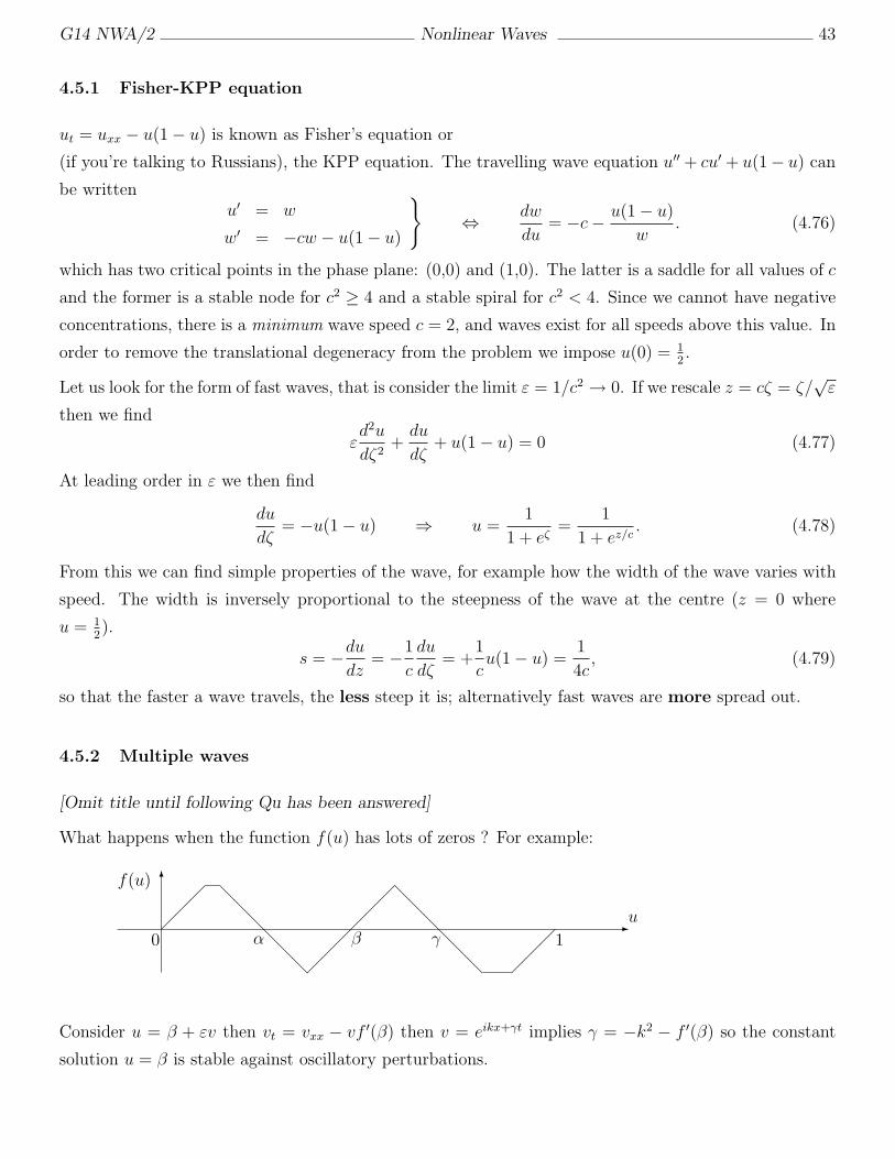
G14 NWA/2 Nonlinear Waves 43
4.5.1 Fisher-KPP equation
ut = uxx − u(1− u) is known as Fisher’s equation or
(if you’re talking to Russians), the KPP equation. The travelling wave equation u′′ + cu′ + u(1− u) can
be writtenu′ = w
w′ = −cw − u(1− u)
}
⇔ dw
du= −c− u(1− u)
w. (4.76)
which has two critical points in the phase plane: (0,0) and (1,0). The latter is a saddle for all values of c
and the former is a stable node for c2 ≥ 4 and a stable spiral for c2 < 4. Since we cannot have negative
concentrations, there is a minimum wave speed c = 2, and waves exist for all speeds above this value. In
order to remove the translational degeneracy from the problem we impose u(0) = 12.
Let us look for the form of fast waves, that is consider the limit ε = 1/c2 → 0. If we rescale z = cζ = ζ/√ε
then we find
εd2u
dζ2+
du
dζ+ u(1− u) = 0 (4.77)
At leading order in ε we then find
du
dζ= −u(1− u) ⇒ u =
1
1 + eζ=
1
1 + ez/c. (4.78)
From this we can find simple properties of the wave, for example how the width of the wave varies with
speed. The width is inversely proportional to the steepness of the wave at the centre (z = 0 where
u = 12).
s = −du
dz= −1
c
du
dζ= +
1
cu(1− u) =
1
4c, (4.79)
so that the faster a wave travels, the less steep it is; alternatively fast waves are more spread out.
4.5.2 Multiple waves
[Omit title until following Qu has been answered]
What happens when the function f(u) has lots of zeros ? For example:
-
6
u
f(u)
@@
@@
@@
@@
@@
@@
0 α β γ 1
Consider u = β + εv then vt = vxx − vf ′(β) then v = eikx+γt implies γ = −k2 − f ′(β) so the constant
solution u = β is stable against oscillatory perturbations.
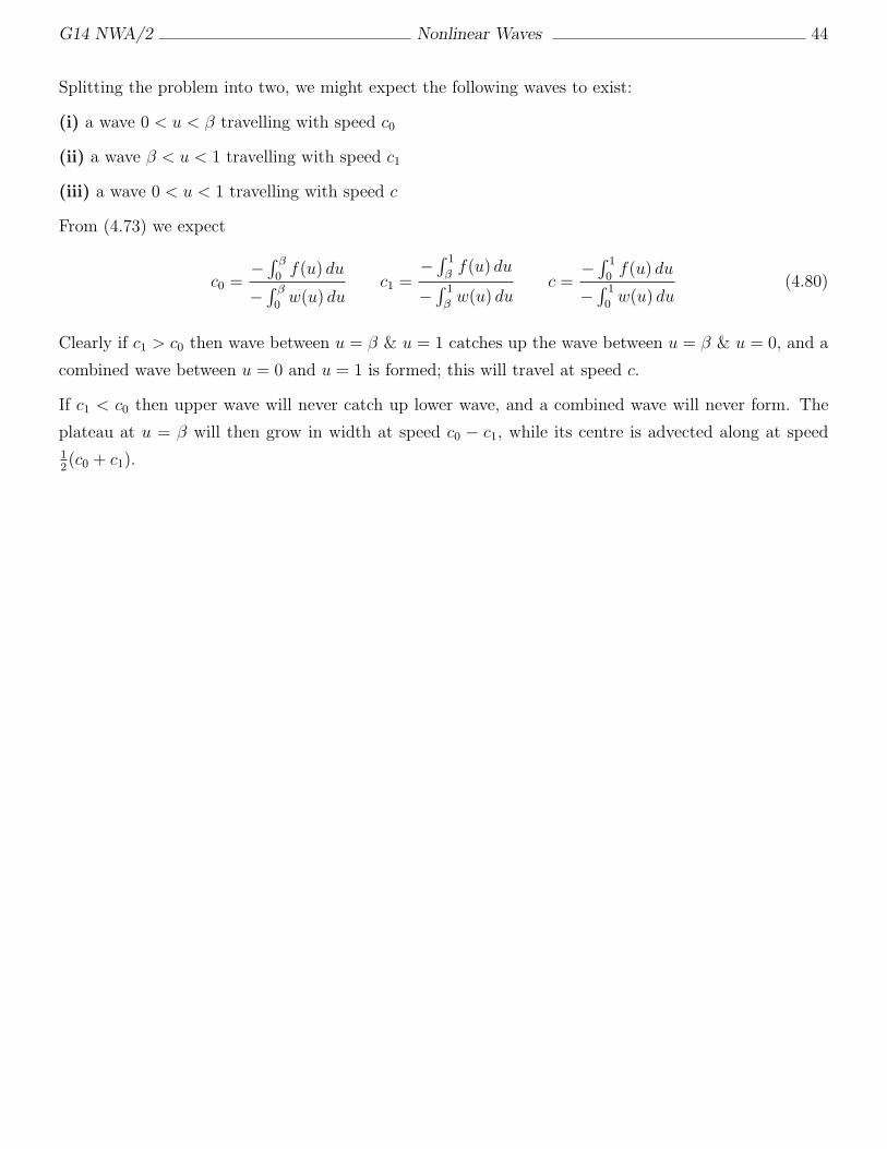
G14 NWA/2 Nonlinear Waves 44
Splitting the problem into two, we might expect the following waves to exist:
(i) a wave 0 < u < β travelling with speed c0
(ii) a wave β < u < 1 travelling with speed c1
(iii) a wave 0 < u < 1 travelling with speed c
From (4.73) we expect
c0 =−∫ β
0f(u) du
−∫ β
0w(u) du
c1 =−∫ 1
βf(u) du
−∫ 1
βw(u) du
c =−∫ 1
0f(u) du
−∫ 1
0w(u) du
(4.80)
Clearly if c1 > c0 then wave between u = β & u = 1 catches up the wave between u = β & u = 0, and a
combined wave between u = 0 and u = 1 is formed; this will travel at speed c.
If c1 < c0 then upper wave will never catch up lower wave, and a combined wave will never form. The
plateau at u = β will then grow in width at speed c0 − c1, while its centre is advected along at speed12(c0 + c1).