Nonlinear System Identification for PredictiveControl using Continuous Time Recurrent

Neural Networks and AutomaticDifferentiation.

R K Al Seyab Y Cao ∗

Cranfield University, UK

Keywords: Nonlinear System, System Identification, Predictive Control,Recurrent Neural Network, Automatic Differentiation.

Abstract

In this paper, a continuous time recurrent neural network (CTRNN)is developed to be used in nonlinear model predictive control (NMPC)context. The neural network represented in a general nonlinear state-space form is used to predict the future dynamic behavior of the non-linear process in real time. An efficient training algorithm for theproposed network is developed using automatic differentiation (AD)techniques. By automatically generating Taylor coefficients, the al-gorithm not only solves the differentiation equations of the networkbut also produces the sensitivity for the training problem. The sameapproach is also used to solve the online optimization problem in thepredictive controller. The proposed neural network and the nonlin-ear predictive controller were tested on an evaporation case study. Agood model fitting for the nonlinear plant is obtained using the newmethod. A comparison with other approaches shows that the newalgorithm can considerably reduce network training time and improvesolution accuracy. The CTRNN trained is used as an internal model ina predictive controller and results in good performance under differentoperating conditions.

∗To whom correspondence should be addressed (y.cao@cranfield.ac.uk).

1 Introduction

Model Predictive Control (MPC) is proving its continuous success in indus-

trial applications particularly in the presence of constraints and varying op-

erating conditions, thereby allowing processes to operate at the limits of their

achievable performance. The basic control strategy in MPC is the selection

of a set of future control moves (control horizon) and minimize a cost func-

tion based on the desired output trajectory over a prediction horizon with

a chosen length. This requires a reasonably accurate internal model, that

captures the essential nonlinearities of the process under control, to predict

multi-step ahead dynamic behavior [1].

In many reported applications of MPC, a linear model is assumed. How-

ever, MPC based on linear models, often results in poor control performance

for highly nonlinear processes because of the inadequateness of a linear model

to predict dynamic behavior of a nonlinear process. There is therefore, a

strong requirement of a good fitting model for NMPC applications.

In many practical applications, a restrict mathematical model based on

physical principles is either unknown or too complicated to be used for con-

trol. In this case, nonlinear system identification is an inevitable step in a

NMPC project. Possibly, it is also the most costly and time consuming part

of the project [2]. Therefore, an efficient and effective approach of nonlinear

system identification is critical to the success of NMPC.

Unlike linear system identification, there is no uniform way to parame-

terize general nonlinear dynamic systems. Among existing techniques, the

universal approximation properties of neural networks makes them a powerful

2

tool for modelling nonlinear systems [3]. The structure of neural networks

may be classified as feedforward and recurrent. Most of the publications

in nonlinear system identification use feedforward neural networks (FFNNs)

with backpropagation or its other variations for training, for example [4, 5].

The main drawback of this approach is that it can only provide predictions

for a predetermined finite number of steps, in most cases, only one step. This

drawback makes such models not well suitable for predictive control, where

variable multi-step predictions are desired.

Recurrent neural networks (RNNs) on the other hand are capable of pro-

viding long range predictions even in the presence of measurements noise [8].

Therefore, RNN models are better suited for NMPC. RNNs with internal

dynamics are adopted in several recent works. Models with such networks

are shown [3, 9], to have the capability of capturing various plant nonlin-

earities. They have been shown more efficient than FFNNs in terms of the

number of neurons required to model a dynamic system [10, 11]. In addition,

they are more suitable to be represented in state-space format, which is quite

commonly used in most control algorithms [12].

In this work, a continuous time version of the recurrent neural networks

(CTRNNs) in state-space form is used as the internal model of NMPC. The

continuous time RNN brings further advantages and computational efficiency

over the discrete formulation even if at the end both are represented on the

computer using only discrete values [13]. Using a discrete time RNNs causes

a great dependence of the resulting models on the sampling period used in the

process and no information is given about the model trajectories between the

sampling instants. The sampling period used with CTRNNs, on the other

3

hand, can be varied without the need for re-training [14, 15].

The main difficulty with recurrent neural networks is their training [13,

16, 17]. Various training strategies have been suggested in the literature,

such as the backpropagation method [18], the conjugate gradient method

[19], Levenberg-Marquardt optimization [20], or methods based on genetic

algorithm (GAs) [21]. To solve the nonlinear optimization problem associated

with CTRNN training, the calculation of a large number of dynamic sensitiv-

ity equations is required. Depending on the number of sensitivity equations

involved, the sensitivity calculation could take more than 90 percent of the

total computation time required for solving a training problem. Hence, sen-

sitivity calculation is a bottleneck in training CTRNNs. Ways to find the

sensitivity of a dynamic system [22] are: perturbation, sensitivity equations,

and adjoint equations. In a perturbation approach, finite difference (FD)

is used to approximate derivatives. Hence at least N perturbations to the

dynamic system are needed to get the solution of a N -parameter sensitivity

problem [22]. Alternatively, sensitivity can also be obtained by simultane-

ously solving the original ordinary differential equations (ODEs) together

with nN sensitivity equations, where n is the number of states [23]. Fi-

nally, sensitivity can be calculated by solving n adjoint equations (in reverse

direction).

Recently, the automatic differentiation (AD) techniques have been ap-

plied to tackle the dynamic optimization problem [24]. In our previous work,

[25], a first-order approximation was derived using AD to simplify the dy-

namic sensitivity equations associated with a NMPC problem so that com-

putation efficiency was improved. In most published work using AD for

4

dynamic optimization, AD has only been used to generate low (first and/or

second) order derivatives. Recently, AD techniques have been used to solve

ODEs and sensitivity equations using high-order Taylor series in a NMPC

formulation [26]. In this work, the approach of [26] is extended to solve both

the CTRNN training and associated NMPC control problems to speed up

calculations and to increase efficiency. Both training and NMPC algorithms

are applied to an evaporator process [27]. The network training time is signif-

icantly reduced by using the new algorithm comparing with other methods.

Using the trained CTRNN as its internal model, the NMPC controller gives

satisfactory control performance at different operating conditions.

The paper is organized as follows. After the introduction, a CTRNN

training algorithm is discussed in section 2. The details of the MPC algorithm

are presented in section 3. Section 4 dedicates to the evaporator case study

including its nonlinear system identification using CTRNN, the predictive

controller design and simulation results. In section 5 some conclusions are

drawn from the work.

5

2 CTRNN Training

2.1 Neural network model

It has been proven that CTRNNs are able to approximate trajectories gen-

erated by nonlinear dynamic systems given by:

x = f(x, u) (1)

y = g(x)

A key to the approximating capabilities of this type of networks is the use of

hidden neurons, [10, 28, 29]. There are many types of neural networks from

multi-layer perceptrons (MLP) to radial basis functions (RBF), which can

be constructed as recurrent networks to approximate the nonlinear system

(1). The training algorithm to be discussed is suitable for any kind networks.

Hence, the CTRNN to be considered is represented in the following general

form.

˙x(t) = f(x(t), u(t), θ) (2)

y(t) = Cx(t)

where u(t) ∈ Rnu is the external input, y ∈ Rny the network output, x ∈ Rnx

the network’s state vector, θ ∈ Rnθ the network parameter vector and the

6

output matrix C is fixed as

C =

[Iny×ny , ∅ny×(nx−ny)

](3)

i.e. outputs are the first ny states of the networks.

A particular example of (2), which will be used for the case study later,

is shown in Figure 2, where a MLP network is adopted to construct the

recurrent neural network of (2).

2.2 CTRNN sensitivity calculation using AD

The definition of the sensitivity is the variation of the network output against

the variation of η, where η ∈ Rnη represents the general parameters, η = θ

in training cases, and η = u(t) in NMPC, whilst in other cases, η may also

include the initial state, x(0). Assume the function f is d-time continu-

ously differentiable. Then, the sensitivity can be calculated by taking partial

derivative for both sides of equations (2):

xη(t) = fxxη(t) + fη (4)

yη(t) = Cxη(t)

where, xη := ∂x/∂η, yη := ∂y/∂η, fx := ∂f/∂x, and fη := ∂f/∂η.

Equation (4) is a linear time-varying system with initial condition, xη(0) =

∂x(0)/∂η. Generally, system (4) has no analytical solution although it can be

represented in a state-transition matrix form [30]. The dynamic sensitivity

7

function xη can be calculated using different method as mentioned earlier.

Numerically, equation (4) can be solved together with the state equation (2)

using a differential equation solver. The total number of differential variables

to be solved at each time instant is nx × (1 + nη). Depend on the size of a

network, this number of differential variables could growth so large that the

calculation causes a significant burden on network training. To tackle this

problem, the sensitivity calculation method proposed in [26] is extended for

CTRNNs.

To solve differential equations (2) and (4), an integration step has to

be determined. Normally, the integration step should be shorter than the

sampling period to get accurate results. However, for the approach devel-

oped here, the accuracy can be maintained by adjusting the Taylor series

order, d. Moreover, for the identification problem, there is no information

available between two sampling points to compare integration results if a

shorter integration step is adopted. Therefore, for simplicity and efficiency,

the integration step is selected to be the same as the sampling period in this

work.

Using normalized time, τ = t/h, where h is the sampling period, the right-

hand-side of the state equation becomes z(x(τ), η(τ)) := hf(x(τ), η(τ)) and

the solution interval is 0 ≤ τ ≤ 1 for each integration step. Consider x(τ)

and η(τ) are given by the truncated Taylor series:

x(τ) = x[0] + x[1]τ + · · ·+ x[d]τd (5)

η(τ) = η[0] + η[1]τ + · · ·+ η[s]τs, s ≤ d (6)

8

with coefficients x[i] ∈ Rnx , and η[i] ∈ Rnη given as follows respectively:

x[i] = (i!)−1∂ix(τ)

∂τ i|τ=0 (7)

η[i] = (i!)−1∂iη(τ)

∂τ i|τ=0 (8)

Let v = [ηT[0] · · · ηT[s]]T , then, z(τ) = z(x(τ), v) can be expressed by a Taylor

expansion:

z(τ) = z[0] + z[1]τ + · · ·+ z[d]τd + O(τ d+1) (9)

where coefficients z[j] is given as;

z[j] = (j!)−1∂jz(τ)

∂τ j|τ=0 (10)

From the chain rule, z[j] is uniquely determined by the coefficient vectors, x[i]

and v with i ≤ j, i.e.

z[j] ≡ z[j](x[0], x[1], · · · , x[j], v) (11)

Nevertheless, inherently, functions z[j] are also d-time continuously differen-

tiable and their derivatives satisfy the identity [31];

∂z[j]

∂x[i]

=∂z[j−i]

∂x[0]

:= A[j−i],x ≡ A[j−i],x(x[0], x[1], · · · , x[j−i], v) (12)

∂z[j−i]

∂v:= A[j−i],v ≡ A[j−i],v(x[0], x[1], · · · , x[j−i], v) (13)

9

where, A[j]x ∈ Rnx×nx , j = 0, · · · , d, and A[j]v ∈ Rnx×snη , j = 0, · · · , d are

also the Taylor coefficients of the Jacobian path, i.e.;

∂z

∂x[0]

= A[0]x + A[1]xτ + · · ·+ A[d]xτd + Oτ d+1 (14)

∂z

∂v= A[0]v + A[1]vτ + · · ·+ A[d]vτ

d + Oτ d+1 (15)

AD techniques provide an efficient way to calculate these coefficients vectors,

z[j] and matrices A[i] [32]. For example, with the software package, ADOL-C

[33, 34], using the forward mode of AD all Taylor coefficient vectors for a

given degree, d can be calculated simultaneously, whilst the matrices, A[i]

can be obtained using the reverse mode of AD. The run time and memory

requirement associated with these calculations grow only as d2.

Using AD for the CTRNN system (2), the Taylor coefficients of x(τ) can

be iteratively determined from x[0] and v [26]:

x[k+1] =1

k + 1z[k](x[0], · · · , x[k], v), k = 0, · · · , d− 1 (16)

y[k] = Cx[k], k = 0, · · · , d (17)

Then, by applying AD to (16), the partial derivatives are obtained and par-

titioned as;

A[k] =

[A[k]x | A[k]v

]:=

[∂z[k]∂x[0]

| ∂z[k]∂v

], (18)

The total derivatives are accumulated from these partial derivatives as fol-

10

lows:

B[k] =

[B[k]x | B[k]v

]:=

[dx[k]

dx[0]| dx[k]

dv

]=

1

k

(A[k−1] +

∑k−1j=1 A[k−j−1]xB[j]

), k = 1, · · · , d (19)

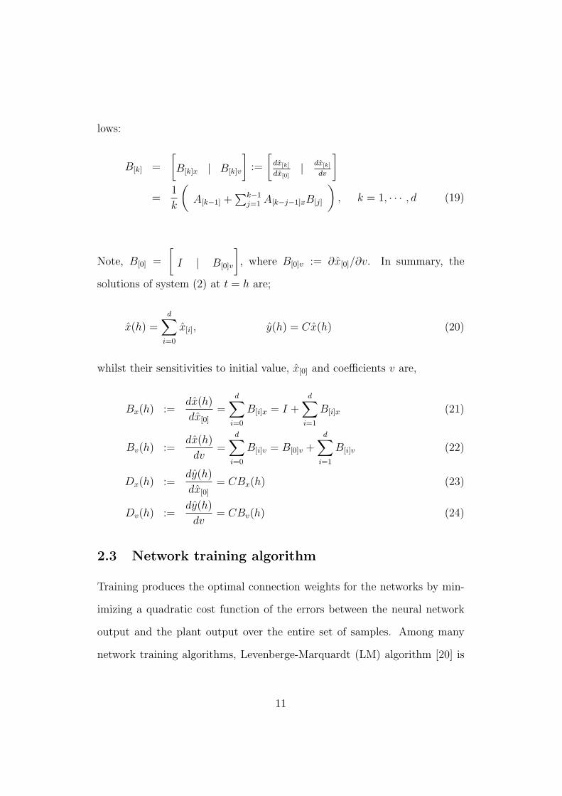
Note, B[0] =

[I | B[0]v

], where B[0]v := ∂x[0]/∂v. In summary, the

solutions of system (2) at t = h are;

x(h) =d∑i=0

x[i], y(h) = Cx(h) (20)

whilst their sensitivities to initial value, x[0] and coefficients v are,

Bx(h) :=dx(h)

dx[0]

=d∑i=0

B[i]x = I +d∑i=1

B[i]x (21)

Bv(h) :=dx(h)

dv=

d∑i=0

B[i]v = B[0]v +d∑i=1

B[i]v (22)

Dx(h) :=dy(h)

dx[0]

= CBx(h) (23)

Dv(h) :=dy(h)

dv= CBv(h) (24)

2.3 Network training algorithm

Training produces the optimal connection weights for the networks by min-

imizing a quadratic cost function of the errors between the neural network

output and the plant output over the entire set of samples. Among many

network training algorithms, Levenberge-Marquardt (LM) algorithm [20] is

11

known to be a robust and fast gradient method because of its second-order

converging speed without having to compute the Hessian matrix. For this

reason, the LM algorithm is combined with the sensitivity algorithm using

AD described above for the dynamic network training.

Firstly, assume the dynamic system (1) is initially at steady-state. By

introducing a set of random inputs to the system, the outputs of the plant are

collected with the inputs for N sampling points at sampling rate h. Then,

the unknown network parameters θ are estimated from the input-output data

set by minimizing the sum of squared approximation errors, i.e.

minθ

Φ = minθ

1

2

N∑i=0

eTi ei (25)

where, ei is the error between the actual plant output and the network output

at i-th sampling point which is a function of the model parameter vector given

by:

ei ≡ ei(θ) = y(ti, θ)− y(ti), i = 1, 2, · · · , N (26)

Let:

E(θ) =

[eT1 · · · eTN

]T(27)

The nyN × nθ Jacobian matrix of E is defined as

J(θ) :=∂E(θ)

∂θ(28)

12

Then, the gradient of Φ is J(θ)E(θ), whilst the Hessian of Φ can be approx-

imated as JT (θ)J(θ). The training algorithm based on the nonlinear least

square approach of Levenberg Marquandt [20] is:

θk+1 = θk −[J(θ)TJ(θ) + µI

]−1

J(θ)TE(θ) (29)

where, θk+1 is an updated vector of weights and biases, θk the current weights

and biases, and I the identity matrix. When the scalar µ is zero, this is a

quasi-Newton approach, using the approximate Hessian matrix, JTJ . When

µ is large, it is equivalent to a gradient descent method with a small step size.

Quasi-Newton method is faster and more efficient when Φ is near the error

minimum. In this way, the performance function Φ will always be reduced

at each iteration of the algorithm.

The Jacobian matrix can be partitioned into N blokes as:

J(θ) = [JT1 (θ) · · · JTN(θ)]T (30)

where each block is an ny × nθ matrix as:

Ji(θ) =∂ei(θ)

∂θ=∂y(ti, θ)

∂θ= C

∂x(ti, θ)

∂θ(31)

For accurate and fast calculation of the sensitivity equations required for

the Jacobian matrix above, the method described in the previous section is

adopted here. Since θ is a constant vector, v = θ.

For given v, x(k + 1) := x(tk+1), and y(k) := y(tk) are iteratively de-

termined from x(0) = [yT (0), 01×(nx−ny)]T using (20). Then the value of

13

Jk(θ) = dy(k)/dv can be calculated using (19) and (21) – (24) as:

Bv(0) = 0 = B[0]v(0) (32)

Bx(k) = I +d∑i=1

B[i]x(k − 1) (33)

Bv(k) = Bv(k − 1) +d∑i=1

B[i]v(k − 1) = B[0]v(k) (34)

Dv(k) = CBv(k) = Jk(θ) (35)

Hence, with AD, the nonlinear training problem can be efficiently solved

using the LM method.

2.4 Model Validation

Many model validity tests for nonlinear models have been developed [35], for

example, the Akaike information criterion (AIC), the statistical χ2 tests, the

predicted squared error criterion, and the higher–order correlation tests.

The most common method of validation is to investigate the residual

(prediction errors) by cross validation on a test data set. Here, validation

is done by carrying out a number of tests on correlation functions, includ-

ing autocorrelation function of the residual and cross-correlation function

between controls and residuals. If the identified model based on CTRNN

is adequate, the prediction errors should satisfy the following conditions of

14

high-order correlation tests [36]:

Ree(τ) = E[e(t− τ)e(t)] = δ(τ), ∀τ (36)

Rue(τ) = E[u(t− τ)e(t)] = 0, ∀τ (37)

where Rxz(τ) indicates the cross-correlation function between x(t) and z(t),

e is the model residual. These tests look into the cross-correlation amongst

model residuals and inputs. These test are normalized to be within a range of

±1 so that the tests are independent of signal amplitude and easy to interpret

[36]. The significance of the correlation between variables is indicated by a

confidence interval. For a sufficiently large data set with length N , the

95% confidence bounds are approximately ±1.96/√N . If these correlation

tests are satisfied (within the confidence limits) then the model residuals are

a random sequence and are not predictable from the model inputs. This

provides additional evidence of the validity of the identified model.

3 Nonlinear predictive control algorithm

Once the CTRNN has been trained, the network can be used as an internal

model of a predictive controller. The recurrent neural network generates

prediction of future process outputs over a specified prediction horizon P ,

15

which allows the following performance criterion to be minimized:

minu≤uk≤u

k=0,...,M−1

ϕ =1

2

P∑k=1

eTy,kQey,k +M∑k=1

∆uTkR∆uk (38)

s.t. ˙x(t) = f(x(t), u(t)), t ∈ [t0, tP ] (39)

y(t) = Cx(t) + d(t) (40)

x(t0) = x0, xk := x(t0 + kh)

uk := u(tk) = u(t), t ∈ [tk, tk+1]

ey,k := yk − rk, k ∈ [1, P ]

∆uk := uk+1 − uk, k ∈ [1,M ]

uk = uM−1, k ∈ [M,P − 1]

where, M and P are the control and prediction horizons respectively, Q ∈

Rny×ny and R ∈ Rnx×nx are the weighting matrices for the output error and

the control signal changes respectively, rk ∈ Rny is the output reference vector

at tk, d is a virtual disturbance estimated at the current time and used to

reduce the model-plant mismatch, u and u are constant vectors determining

the input constraints as element-by-element inequalities.

The prediction horizon [t0, tP ] is divided into P intervals, t0, t1, · · · , tP

with ti+1 = ti + hi and∑P−1

i=0 hi = tP − t0. For piecewise constant control,

assume the optimal solution to (38) is u(t) ≡ u(tk) = u[0](k) for tk ≤ t ≤ tk+1,

k = 0, · · · , P − 1. Then, only the solution in the first interval is to be

implemented and whole procedure will be repeated at next sampling instant.

Let v ∈ RM×nu be defined as v := [uT[0](0) · · ·uT[0](M − 1)]T . Problem (38)

is a standard nonlinear programming problem (NLP) which can be solved

16

by any modern NLP solvers. To efficiently solve the online optimization

problem of the predictive controller the same gradient calculation strategy

of the NMPC approach proposed by [26] is used.

A simple method is used to estimate the initial value of the model states

required to solve the optimization problem at each sample time. In this

method, the new states are updated from the old values using the dynamic

equation (39). Also, the state estimate error was reduced further by adding

the virtual disturbance d to the output. No terminal penalty is used in this

work and a good tuning of h, P , M , Q, and R was found enough to ensure

the close-loop stability for the case study in different operation conditions.

4 Case Study – An Evaporator Process

This case study is based on the forced-circulation evaporator described by

Newell and Lee [27], and shown in Figure 1. In this process, a feed stream

enters the process at concentration X1 and temperature T1, with flow rate F1.

It is mixed with recirculating liquor, which is pumped through the evaporator

at a flow rate F3. The evaporator itself is a heat exchanger, which is heated

by steam flowing at rate F100 with entry temperature T100 and pressure P100.

The mixture of feed and recirculating liquor boil inside the heat exchanger,

and the resulting mixture of vapour and liquid enters a separator where the

liquid level is L2 . The operating pressure inside the evaporator is P2. Most

of the liquid from the separator becomes the recirculating liquor. A small

proportion of it is drawn off as product, with concentration X2, at a flow rate

F2 and temperature T2. The vapour from the separator flows into a condenser

17

at flow rate F4 and temperature T3, where it is condensed by cooling water

flowing at rate F200, with entry temperature T200 and exist temperature T201.

The nominal values of the system variables are given in Table 1, while the

first-principle model equations are available in [27].

4.1 System identification using CTRNN

The evaporator system has been adopted as a case study for system identifica-

tion using CTRNN by a group of researchers [15], where a Genetic Algorithm

(GA) based approach was used to train the CTRNN as it was believed that

“the implementation of gradient-based training algorithms is computation-

ally expensive”. However, only a short period (5 minutes) of data with simple

input signals (step changes) was used to train the network and another short

period (7.5 minutes) was adopted for model validation. In this work, it is

to be demonstrated that with the approach developed above the gradient-

based algorithm is not computationally expensive any more comparing with

the GA based approach since the new training algorithm is able to handle a

much longer period (500 minutes) of data with much more complicated input

signals (random pulses) for training and validation.

The evaporator is approximated using a continuous-time recurrent MLP

18

network with one hidden layer as shown in Figure 2:

xh(t) = σs (Wxx(t) +Wuu(t) + b1) (41)

˙x(t) = W2xh(t) + b2

y(t) = Cx(t)

where, Wx ∈ Rnh×nx , Wu ∈ Rnh×nu , andW2 ∈ Rnx×nh are connection weights,

b1 ∈ Rnh and b2 ∈ Rnx are bias vectors, whilst each element of the vector

σs(·) ∈ Rnh represents the sigmoid-tanh function as the neural activation

function, i.e.

σs(n) =2

1 + e−2n− 1 (42)

The parameter vector is θ =

[vec(Wx)

T vec(Wu)T bT1 vec(W2)

T bT2

]T∈

Rnθ , where nθ = nx× (nh+1)+nh× (nx+nu+1). The identification scheme

assumes that the plant model equations are unknown and the only available

information is the input-output data which is generated through various runs

of the first principle model of the plant given by [27]. Two different structures

of the CTRNN are studied to model the process. The first network (Network

1) was trained with nx = ny = 3, and nh = 8 (nθ = 83), while the second

one (Network 2) was trained with nx = 5 and nh = 8 (nθ = 117). The

training was carried out repetitively over the data collected within a fixed

time interval of 500 minutes and sampled at every 0.2 minutes. The inputs

training data was a random pulses with a different amplitude and durations

19

with the range chosen to cover all the region of operation of the plant (see

Figure 3). Another set of data at sampling time 0.05 minutes is randomly

generated from the plant to be used for network validation. The output data

are corrupted with a normally distributed zero mean noise with variance 5%

of the steady state values of the output variables. The initial values of the

first ny network states were chosen equal to the steady state values of the

simulated plant outputs while the (nx − ny) remains were equal to zeros.

To demonstrate the CTRNN capability for evaporator model approxi-

mation, the simulated plant output and the trained neural networks output

are compared in figures 4 and 5. A good model fitting is observed for both

networks with approximately similar accuracy with the training data. In

terms of model validation, Network 1 is better than Network 2 as shown in

Figure 5. This means increase the network state dimension does not neces-

sarily improve the model fitting. Sometimes, networks with high order could

include undesirable eigenvalues which may induce an unstable or poor perfor-

mance. Therefore, Network 1 is chosen as the internal model of the predictive

controller for accurate and fast online calculations. Also, the validation re-

sults show the capability of the network to approximate the simulated plant

output with a sampling time less than that used for training, without the

need to re-train the network. In fact, this is one of the most important

advantages of CTRNNs over discrete-time recurrent networks.

Also, as a confidence test of the resulting model, the correlation–based

model validation results for the CTRNN model can be calculated according

to equations (36)–(37) and shown in figures 6 and 7 respectively. The dotted

lines in each plot are the 95% confidence bounds (±1.96/√

500). It can be

20

seen that only a small number of points are outside the bounds. This demon-

strates that the model can be considered as being adequate for modelling this

plant.

To solve the training problem, a total nx × N × nθ = 3 × 2000 × 83 =

498000 sensitivity variables have to be calculated in addition to the original

3 ordinary differential equations (ODEs) of Network 1 while for Network 2,

the number of sensitivity is 5 × 2000 × 117 = 1170000. To demonstrate the

efficiency of the new algorithm, it is compared with the traditional sensitivity

equation integrating approach using a typical numerical ODE solver, the

MATLAB function ode15s.

To compare computation time associated with a given accuracy, a refer-

ence solution is produced by using ode15s solver and setting the error toler-

ance to 10−14. Then with four tolerance settings, (10−3, 10−6, 10−8, 10−10)

and four different Taylor series orders (3, 6, 8, 10), computation time and

accuracy against the reference solutions using two different approaches are

compared in Table 2. A third network (Network 3) with new configurations

(nx = 4, nh = 15, and sensitivity variables number = 4 × 2000 × 169 =

1352000) has been trained and the results are given in Table 2 for com-

parison. Note that the computation time in Table 2 is the time required to

calculate the cost function and the sensitivity variables over one optimization

iteration whilst the error term in the same table is the maximum absolute

error against the reference solution. The table shows that training algorithm

using AD perform better than the traditional sensitivity approach in both

efficiency and accuracy. It can be seen that the order of Taylor series plays an

important role in error control. Increase the order by a few number, the error

21

would be reduced by a number of orders magnitude without increasing too

much computation time. However, using traditional approaches, significant

computation time may have to be traded off for a reduction in computation

error. A way to determine an appropriate order of Taylor series for a given

error tolerant was suggested in [26]. It is worth to mention that a successful

training would require thousands of iterations. If the accuracy of ODE solver

is lower, it would require even more iterations to get a converged solution.

Therefore, the time comparison listed in Table 2 suggests a massive efficiency

improvement in network training achieved by the proposed approach.

All tests are done on a Windows XP PC with an Inetl Pentium-4 processor

running at 3.0 GHz. Note that, the proposed algorithm is implemented in C

using ADOL-C and interfaced to MATLAB via a mex warp.

4.2 Evaporator predictive control

Effective control of the evaporator system using traditional PID controllers

was not very successful especially for large setpoint changes [27]. Predictive

control was also considered by a number of workers. Linear model predic-

tive control (LMPC) was demonstrated to be not sufficient to fully control

this process for an excessive range of variation (see control objectives given

bellow)[37] (see Figure 8). A nonlinear MPC strategy based on successive

linearization solution to control this process under a large setpoint change

condition was proposed by Maciejowski [37]. A good performance was ob-

served after re-linearizing the nonlinear process model after every few steps.

However, disturbances have not been considered there. In this paper, the

22

NMPC algorithms described in section 3 is applied to control the process for

setpoint tracking and disturbance rejection tests described as follows;

The control objective of the case study is;

1. Track setpoint ramp changes of X2 from 25% to 15% and P2 from 50.5

kPa to 70 kPa.

2. Track setpoint changes as above when unmeasured disturbances, F1,

X1, T1 and T200 are varied within ±20% of their nominal values.

The control system is configured with three manipulated variables, F2, P100

and F200 and three measurements, L2, X2 and P2. All manipulated variables

are subject to a first order lag with a time constant equal to 0.5 minutes and

saturation constraints, 0 ≤ F2 ≤ 4, 0 ≤ P100 ≤ 400 and 0 ≤ F200 ≤ 400.

To tune control horizon M , prediction horizon P , and sampling time h,

initially let P = M = 1 min, and h = 1 min. By varying M (and assuming

P = M) from 1 to 15 min, a stable performance is obtained which satisfies

all control specifications for 1 ≤ M ≤ 20 min. When M ≥ 10 min, the

improvement on the system performance is negligible but computation time

increases. Therefore M = 4 min is selected. The same steps are used to

choose a suitable prediction horizon P , a reasonable range from the minimum

value (P = M = 1) min to P = 40 min has been tested. A stable response

without any constraints violation is detected within range 1 ≤ P min. No

performance improvement can be observed when P ≥ 7 min. Therefore

P = 7 min is chosen to ensure that both the system stability and satisfactory

control performance achieved within a reasonable computation time.

The weighting matrix, Q = diag(Q0, · · · , Q0), where Q0 is diagonal and

23

initially set to be the inverse of the output error bounds. After online tuning,

the final values are:

Q0 =

1000 0 0

0 500 0

0 0 200

(43)

Also, the input weighting matrix R = diag(R0, · · · , R0), where R0 is diagonal

and set to I.

By using piecewise constant input, the result NLP problem has nu ×

M = 12 degrees of freedom. To solve the NLP problem of the NMPC, a

total (nx × P ) × (nu × M) = 252 sensitivity variables have to calculated

in addition to original 3 ODEs of the neural network. In this work, the

sensitivity equations are solved using the sensitivity algorithm of [26].

4.3 Simulation Results

Simulation results of all tests above are shown in figures 8 and 9. The effi-

ciency and the stability of the proposed CTRNN based NMPC during set-

point ramp test has been proved in contrast with the LMPC [37] as shown

in Figure 8. Also, it can be seen from the results given in Figure 9 that mea-

sured outputs follow the setpoints quite well without any input constraints

violation in spite of the existence of severe unmeasured disturbances.

To test the controller sensitivity to the sampling time, simulations have

also been done by varying h from 0.5 min to 2 min. A stable performance

without constraints violation at all tests are also obtained. Knowing that

24

the recurrent neural network (Network 1) which is trained at h = 0.2 min is

used as the controller internal model at all the above tests.

A detailed stability analysis for nonlinear model predictive control of the

evaporator has been done [38], where using the new stability measure de-

veloped, a concrete conclusion had been obtained, i.e. the NMPC of the

evaporator is asymptotically stable around the nominal steady state for any

positive definite state weighting matrix, Q. The work also provided a way to

calculate the stability region around the nominal steady state. According to

[38], it can be shown that the NMPC described in this work is always stable.

5 Conclusion

This paper demonstrates the reliability of artificial neural networks in pro-

cess control. An efficient algorithm has been proposed to train continuous-

time recurrent neural networks to approximate nonlinear dynamic systems

so that the trained network can be used as the internal model for a nonlinear

predictive controller. The new training algorithm is based on the efficient

Levenberge Marquardt method combined with an efficient and accurate tool:

automatic differentiation. The dynamic sensitivity equations and the ODEs

of the recurrent neural network are solved accurately and simultaneously via

AD. Big time saving to solve sensitivity equations with a higher accuracy

are observed using the new algorithm compared with a traditional method.

Also, the trained networks with a different model orders show the capability

to approximated the multivariable nonlinear plant at different sampling time

without the need to re-train the networks. The results show that, the choice

25

of the network order is also very important to get a good model fitting and

stable performance. Based on the identified neural network model, a NMPC

controller has been developed. The similar strategy that used in the network

training has been used to solve the online optimization problem of the predic-

tive controller. The capability of the new nonlinear identification algorithm

and NMPC algorithm are demonstrated via an evaporator case study with

satisfactory results.

References

[1] Pearson R. K., “Selecting Nonlinear Model Structures for Computer Con-

trol: Review”, Journal of Process Control, vol. 13, pp. 1-26, 2003.

[2] Zhao H., Guiver J., and Sentoni G., “An Identification Approach to Non-

linear State Space Model for Industrial Multivariable Model Predictive

Control”, Proceeding of the American Control Conference, Philadelphia,

Pennsylvania, 1998.

[3] Funahashi K. L. and Nakamura Y., “Approximation of Dynamical Sys-

tems by Continous time Recurrent Neural Networks”, Neural Networks,

vol. 6, pp. 183 – 192, 1993.

[4] Temeng H., Schenelle P., and McAvoy T., “Model Predictive Control of

an Industrial Packed Reactors using Neural Networks”, J. Proc. Control,

vol. 5(1), pp. 19 – 28, 1995.

26

[5] Tan Y., and Cauwenberghe A., “Nonlinear One Step Ahead Control us-

ing Neural Networks:Control Strategy and Stability Design”, Automatica,

vol. 32(12), pp. 1701 – 1706, 1996.

[6] Miller W. T., Sutton R. S., and Werbos P. J., ”Neural Networks for

Control”, MIT Press, Cambridge, MA, 1990.

[7] Narendra K. S. and Parthasarathy K., ”Identification and Control of Dy-

namical Systems using Neural Networks”, IEEE Trans, Neural Networks,

vol. 1(1), pp. 4 – 26, 1990.

[8] Su H. T. and McAvoy T. J., “Artificial Neural Networks for Nonlinear

Process Identification and Control”, Nonlinear Process Control, M. A.

Henson and D. E. Seborg (eds) Prentic Hall, NJ, pp. 371 – 428, 1997.

[9] Jin L., Nikiforuk P. , Gupta M., “Approximation of Discrete-Time State-

space Trajectories using Dynamic Recurrent Neural Networks”, IEEE

Transactions on Automatic Control, vol. 40(7), pp. 1266-1270, 1995.

[10] Delgado A., Kambhampati C., Warwick K., “Dynamic Recurrent Neu-

ral Network for System Identification and Control”, IEE Proc. Control

Theory Appl., vol. 142(4), pp. 307-314. 1995.

[11] Hush D. R. and Horne B. G., “Progress in Supervised Neural Networks”,

IEEE Sig. Process, Mag., vol. 1, pp. 8 – 39, 1993.

[12] Zamarreno J. M. and Vega P., “State-Space Neural Network, Properties

and Application”, Neural Networks, vol. 11, pp. 1099 – 1112, 1998.

27

[13] Pearlmutter B. A., “Gradient Calculations for Dynamic Recurrent Neu-

ral Networks: A Survey”, IEEE Transactions on Neural Networks, 1995.

[14] Kambhampati C., Craddock R. J., Tham M., Warwick K., “Inverse

Model Control using Recurrent Networks”, Mathematics and Computers

in Simulation, vol. (51), pp. 181-199, 2000.

[15] Kambhampati C., Garces F., Warwick K., “Approximation of Non-

autonomouous Dynamic Systems by Continuous Time Recurrent Neu-

ral Networks”, Proceeding of the IEEE-INNS-ENNS International Joint

Conference on Neural Networks IJCNN 2000, vol. 1, pp. 64 – 69, 2000.

[16] Kambhampati C., Manchanda S., Delgado A., Green G., Warwick K.,

Tham M., “The Relative Order and Inverses of Recurrent Networks”,

Automatica, vol. 32(1), pp. 117-123, 1996.

[17] Prasad V., and Bequette B. W., “Nonlinear System Identification and

Model Reduction using Artificial Neural Networks”, Computers and

Chemical Engineering, vol. 27, pp. 1741-1754, 2003.

[18] Rumelhart D. E., Hinton G. E., and Williams R. J., “Learning Internal

Representiations by Error Propagation”, in Prallel Distributed Process-

ing, D. E. Rumelhart and J. L. MeClelland, Eds., Cambrige MA:MIT

Press, 1986.

[19] Leonard J. A. and Kramer M. A., “Improvement of the Back-

propagation Algorithm for Training Neural Networks”, Computers and

Chemical Eng., vol. 14, pp. 337 – 341, 1990.

28

[20] Marquardt D., “An Algorithm for least-Square Estimation of Nonlinear

Parameters” SIAM J. Appl. Math., vol. 11 , pp. 431 – 441 , 1963.

[21] Goldberge D. E., “Genetic Algorithms in Search, Optimization and Ma-

chine Learning”, Reading, MA:Addision-Wesley, 1989.

[22] Storen S., Hertzberg T., “Obtaining Sensitivity Information in Dynamic

Optimization Problems Solved by the Sequential Approach”, Computer

and Chemical Engineering, vol. 23, pp. 807 – 819, 1999.

[23] Schlegel M., Marquardt W., Ehrig R., Nowak U., “Sensitivity Analysis

of Linearly Implicit Differential-Algebraic Systems by One-step Extrap-

olation”, Applied Numerical Mathematics, vol. 48, pp. 83 – 102, 2004.

[24] Griesse R., Walther A., “Evaluating Gradients in Optimal Control: Con-

tinuous Adjoint Versus Automatic Differentiation”, Journal of Optimiza-

tion Theory and Applications, vol. 122(1), pp. 63 – 86, 2004.

[25] Cao Y., and A-Seyab R., “Nonlinear Model Predictive Control using

Automatic Differentiation”, European Control Conference (ECC 2003),

Cambridge, UK, 2003, p. in CDROM.

[26] Cao Y.,“A Formulation of nNonlinear Model Predictive Control using

Automatic Differentiation”, Journal of Process Control, vol. 15, pp. 851

– 858, 2005.

[27] Newell R. B. and P. L. Lee, “Applied Process Control-A Case Study”,

Prentice Hall, Englewood Cliffs, NJ, 1989.

29

[28] Garces F., Kambhampati C., and Warwick K., “Dynamic Recurrent

Neural Networks for Identification of a Multivariable Nonlinear Evapora-

tor Systems”, Proceedings DYCONS’99, World Scientific, 1999.

[29] Garces F., Kambhampati C., and Warwick K., “Dynamic Recurrent

Neural Networks for Feedback Linearization of a Multivariable Nonlinear

Evaporator Systems”, In Review for UKACC International Conference

Control, 2000.

[30] Chen C. T., “Linear System Theory and Design”, third ed., Oxford Uni-

versity Press, New York, 1999.

[31] B. Christianson, “Reverse Accumulation and Accurate Rounding Error

Estimatres for Taylor Series”, Optimization Methods and Software, vol. 1,

pp. 81 – 94, 1992.

[32] Griewank A., ”Evauating Derivatives”, SIAM, Philadelphia, PA, 2000.

[33] Griewank A., David J., Jean U., “ADOL-C: A Package for the Auto-

matic Differentiation of Algorithms written in C/C++”, ACM Transac-

tions on Mathematical Software, vol. 22(2), pp. 131 – 167, 1996.

[34] Griewank A., “ODE Solving via Automatic Differentiation and Ratio-

nal Prediction”, in: Griffiths D., Watson G. (Eds.), Numerical Analysis

1995, vol. 344 of Pitman Research Nots in Mathematics Series, Addison-

Wesley., Reading, MA, 1995.

30

[35] Zhang J., and Morris J., “Recurrent neuro–fuzzy networks for nonlinear

process modeling”, IEEE Trans. on Neural Networks, vol. 10(2), pp. 313–

326, 1999.

[36] Billings S. A. and Voon W. S. F., “Correlation based model validity

tests for nonlinear models”, Int. J. Control, vol. 44, pp. 235–244, 1986.

[37] Maciejowski J. M., “Predictive control with constraints”, Prentice Hall,

Harlow, England, 2002.

[38] Chen, W.-H. and Cao, Y., “Stability analysis of constrained nonlinear

model predictive control with terminal weighting”, submitted to Interna-

tional Journal of Robust and Nonlinear Control, 2007.

31

List of Figures

1 Evaporator System . . . . . . . . . . . . . . . . . . . . . . . . 33

2 Recurrent Neural Network Structure . . . . . . . . . . . . . . 34

3 Training data set, Inputs, 4T = 0.2 min. . . . . . . . . . . . . 35

4 Training data set, Outputs, 4T = 0.2 min. . . . . . . . . . . . 36

5 Validation data set, Outputs, 4T = 0.05 min. . . . . . . . . . 37

6 Validation tests/Autocorrelation coeff. for error, 4T = 0.05

min. . . . . . . . . . . . . . . . . . . . . . . . . . . . . . . . . 38

7 Validation tests/Cross-correlation coef. of U, 4T = 0.05 min. 39

8 Evaporator performance at setpoints ramp changes using LMPC

[37] and the proposed NMPC, 4T = 1 min. . . . . . . . . . . 40

9 Evaporator performance using the present NMPC at setpoint

changes plus random disturbances test. (a)–(c) Measured out-

puts with setpoints. (d)–(f) Manipulated variables. (g)–(j)

Disturbances, 4T = 1 min. . . . . . . . . . . . . . . . . . . . 41

32

Steam T100F100 P100

Evaporator

Condensate

FeedF1, X1, T1

F3

SeparatorP2, L2

ProductF2, X2, T2

T201

T200 F200

CoolingwaterCondenser

Figure 1: Evaporator System

33

)(ˆ ty∫

)(⋅sσ

)(⋅sσ

)(⋅sσ

)( tu

)(ˆ tx

)(⋅sσ

)(ˆ tx&C

M

2W

Input layer Hidden layer Output layer

1b

2b

x

u

W

W

Figure 2: Recurrent Neural Network Structure

34

0 50 100 150 200 250 300 350 400 450 500

0

1

2

3

4

F2, k

g/m

in

0 50 100 150 200 250 300 350 400 450 50050

100

150

200

250

300

P10

0, kP

a

0 50 100 150 200 250 300 350 400 450 5000

50

100

150

200

250

300

F20

0, kg/

min

time, minutes

Figure 3: Training data set, Inputs, 4T = 0.2 min.

35

0 50 100 150 200 250 300 350 400 450 5000

1

2

3

4

5

6

L 2, m

0 50 100 150 200 250 300 350 400 450 5000

10

20

30

40

50

60

X2, %

0 50 100 150 200 250 300 350 400 450 50020

30

40

50

60

70

80

90

P2, k

Pa

time, minutes

Actual outputNetwork 1 outputNetwork 2 output

Figure 4: Training data set, Outputs, 4T = 0.2 min.

36

0 50 100 150 200 250 300 350 400 450 5000

1

2

3

4

5

6

7

L 2, m

0 50 100 150 200 250 300 350 400 450 5000

10

20

30

40

50

60

X2, %

0 50 100 150 200 250 300 350 400 450 50020

30

40

50

60

70

80

90

P2, k

Pa

time, minutes

Actual outputNetwork 1 outputNetwork 2 output

Figure 5: Validation data set, Outputs, 4T = 0.05 min.

37

0 5 10 15 20 25−1

−0.5

0

0.5

1

0 5 10 15 20 25−1

−0.5

0

0.5

1

0 5 10 15 20 25−1

−0.5

0

0.5

1

lag

Re 1e 1(τ

)R

e 2e 2(τ)

Re 3e 3(τ

)

Network 1

Network 2

Figure 6: Validation tests/Autocorrelation coeff. for error, 4T = 0.05 min.

38

−20 −10 0 10 20−1

−0.5

0

0.5

1

−20 −10 0 10 20−1

−0.5

0

0.5

1

−20 −10 0 10 20−1

−0.5

0

0.5

1

lag

−20 −10 0 10 20−1

−0.5

0

0.5

1

−20 −10 0 10 20−1

−0.5

0

0.5

1

−20 −10 0 10 20−1

−0.5

0

0.5

1

lag

RU

e 1(τ)

RU

e 1(τ)

RU

e 2(τ)

RU

e 2(τ)

RU

e 3(τ)

RU

e 3(τ)

Network 1 Network 2

Ru

3e

1

Ru1e

1

Ru

2e

1

Figure 7: Validation tests/Cross-correlation coef. of U, 4T = 0.05 min.

39

0.8

1

1.2

1.4

1.6

L 2, m

14

16

18

20

22

24

26

X2, %

0 20 40 60 80 10050

55

60

65

70

75

P2, k

Pa

time, min.

0

1

2

3

4

F2, k

g/m

in

0

100

200

300

400

P10

0, kP

a

0 20 40 60 80 1000

100

200

300

400

time, min.

F20

0, kg/

min

LMPCSetpointNMPC

Output Variables Input Variables

Figure 8: Evaporator performance at setpoints ramp changes using LMPC[37] and the proposed NMPC, 4T = 1 min.

40

0.8

1

1.2

1.4

L2, m

a

10

15

20

25

30

X2,

%

b

50

60

70

80

P2,

kP

a

c

0

1

2

3

4

F2,

kg/

min

d

0

100

200

300

400

P10

0, k

Pa

e

0

100

200

300

400

F20

0, k

g/m

in

f

8

9

10

11

12

F1,

kg/

min

g

4

4.5

5

5.5

6

X1,

%

h

0 20 40 60 80 10030

35

40

45

50

time, min

T1,

o C

i

0 20 40 60 80 10020

25

30

time, min

T20

0, o C

j

Figure 9: Evaporator performance using the present NMPC at setpointchanges plus random disturbances test. (a)–(c) Measured outputs with set-points. (d)–(f) Manipulated variables. (g)–(j) Disturbances, 4T = 1 min.

41

Table 1: Evaporator Variables and ValuesVariables Description Nominal value UnitsF1 Feed flowrate 10 kg/minF2 Product flowrate 2.0 kg/minF3 Circulating flowrate 50 kg/minF4 Vapor flowrate 8.0 kg/minF5 Condensate flowrate 8 kg/minX1 Feed composition 5.0 %X2 Product composition 25 %T1 Feed temperature 40.0 %T2 Product temperature 84.6 oCT3 Vapor temperature 80.6 oCL2 Separator level 1.0 mP2 Operator pressure 50.5 kPaF100 Steam flowrate 9.3 kg/minT100 Steam temperature 119.9 oCP100 Steam pressure 194.7 kPaQ100 Heat duty 339 kWF200 Cooling water flowrate 208 kg/minT200 Inlet C. W. temperature 25.0 oCT201 Outlet C. W. temperature 46.1 oCQ200 Condenser duty 307 kW

42

Table 2: Computing Time and Accuracy ComparisonTraditional Sensitivity Approach

Tolerance Network 1 Network 2 Network 3Time, ms Error Time, ms Error Time, ms Error

10−3 13.859 0.555 48.328 4.7175 67.641 0.585110−6 45.046 0.0153 257.454 0.1351 459.046 0.013510−8 69.437 4.0183×10−4 434.547 8.973×10−4 740.688 2.1924×10−4

10−10 77.906 1.1103×10−8 580.125 1.3316×10−5 838.563 9.6209×10−9

ADOL–C Software

Order Network 1 Network 2 Network 3Time, ms Error Time, ms Error Time, ms Error

3 2.609 3.276×10−5 3.11 1.396×10−4 4.157 1.9759×10−5

6 4.031 2.095×10−10 5.281 1.7862×10−9 6.844 7.5623×10−9

8 5.207 1.136×10−13 6.875 1.2301×10−12 9.234 6.7502×10−11

10 6.813 8.881×10−16 8.875 5.6843×10−14 12.609 7.9543×10−14

43