Embed Size (px)
Citation preview

Tomas Bata University in Zlín Faculty of Applied Informatics
Nonlinear System Identification
and Control Using Local Model
Networks
Jakub Novák, Ing.
February 2007

2
Acknowledgment
This dissertation is the result of my research activities at the Tomas Bata
University in Zlín, Faculty of Applied Informatics, department of Process Control.
I would like to express my heartiest gratitude to my supervisor Professor
Vladimír Bobál for his support in all phases of this work. I owe a lot to my colleagues
at the faculty. They always helped me through discussion and suggestions. Special
thanks in this regards to Petr Chalupa.
Finally, I would like to thank my parents for their love, support and
understanding.

3
Contents
Chapter 1 INTRODUCTION......................................................................... 12
1.1 Background........................................................................................ 12
1.2 Aims of thesis .................................................................................... 16
1.3 Overview of thesis ............................................................................. 16
Chapter 2 LOCAL MODEL NETWORKS.................................................. 18
2.1 Introduction........................................................................................ 18
2.2 Radial Basis Network ........................................................................ 19
2.3 RBF-ARX Model............................................................................... 21
2.4 Local Model Networks ...................................................................... 22
2.5 Validity functions .............................................................................. 25
2.6 Side-effects of the normalization of validity functions ..................... 26
2.7 Local Models ..................................................................................... 28
2.8 Affine modelling................................................................................ 29
2.9 Fuzzy-based local modelling ............................................................. 30
2.10 Concluding remarks......................................................................... 31
Chapter 3 NONLINEAR SYSTEM MODELLING USING LOCAL
MODEL NETWORKS ................................................................................... 32
3.1 Divide and Conquer Strategy ............................................................ 33
3.2 The modelling process ....................................................................... 34

4
3.3 Structural identification...................................................................... 36
3.4 Heuristic strategies for structure identification .................................. 38
3.4.1 Johansen and Foss Algorithm..................................................... 39
3.4.2 LOLIMOT algorithm.................................................................. 41
3.5 Structure optimization via the SOMA algorithm ............................... 41
3.6 Parameter Estimation in Local Model Network Structure ................. 43
3.7 Global learning................................................................................... 43
3.8 Local Learning ................................................................................... 45
3.9 Incorporating a priori knowledge ...................................................... 46
3.10 Validation......................................................................................... 49
3.11 Concluding Remarks........................................................................ 49
Chapter 4 CONTROLLER DESIGN BASED ON LOCAL LINEAR
MODEL DESCRIPTION ............................................................................... 51
4.1 Local Controller Networks................................................................. 52
4.2 Model Predictive Control ................................................................... 53
4.3 Nonlinear Model Predictive Control .................................................. 55
4.4 Single-model predictions ................................................................... 56
4.5 Multi-model predictions..................................................................... 59
4.6 Internal Model Control based on Local Linear Models ..................... 61
4.7 Concluding Remarks .......................................................................... 63
Chapter 5 SIMULATION AND EXPERIMENTAL STUDIES ................. 64
5.1 Simulation Studies ............................................................................. 64
5
5.2 pH Neutralization Plant ..................................................................... 64
5.3 Structure and Parameter Identification of the Local Model Network 68
5.4 Predictive Control using LMN .......................................................... 77
5.5 Nonlinear Model Predictive Control.................................................. 78
5.6 Internal Model Control using LMN................................................... 79
5.7 Laboratory Experiments .................................................................... 82
5.8 Nonlinear Modelling and Control of the Two-tank System .............. 83
5.9 Internal Model Control of Two-tank system ..................................... 86
5.10 Discussion and Concluding Remarks .............................................. 87
Chapter 6 Concluding Summary and Future Work.................................... 89
Publications.............................................................................................. 97

6
Nomenclature
Acronyms
ARX AutoRegressive with eXogeneous inputs
ASMOD Adaptive Spline Modelling of Observation Data
BFGS Broyden-Fletcher-Goldfarb-Shanno method
CSTR Continuous Stirred Tank Reactor
GMV Generalized Minimum Variance
EM Expectation Maximization algorithm
J&F construction algorithm of Johansen and Foss
LLC Local Linear Controller
LLM Local Linear Model
LMN Local Model Network
LOLIMOT Local Linear Model Tree
MLP Multiple Layer Perceptron
MPC Model Predictive Control
MMPC Multiple Model Predictive Control
NARX Nonlinear Auto Regressive with eXogenous input
QP Quadratic Programming
RBF Radial Basis Function
RLS Recursive Least-Squares
SVD Singular Value Decomposition

7
General Notations
, ,a b Scalars
a,b,θ Vectors
A,B,… Matrices
( ), ( )A z B s Polynomials
Functions and Operators
Variables
a parameter vector of the local model
A denominator polynomial of a system
b parameter vector of the local model
B numerator polynomial of a system
c centre of the validity function
e estimation error
cH control horizon
pH prediction horizon
J objective or cost function
M number of models
na number of maximum lags in output signal
nb number of maximum lags in input signal
width of the validity function
θ
vector of parameter estimates
ρ normalised validity function

8
unnormalised validity function
φ regression vector
ψ vector of scheduling variables

9
List of Figures
Figure 1 RBF network............................................................................................. 20
Figure 2 Local Model Network scheme.................................................................. 23
Figure 3 The nonlinear input/output approximation (c) is obtained by
combining three linear models (a) with validity functions (b)........................ 24
Figure 4 Effect of varying width, 2 , for 2-dimensional Gaussian validity
function ........................................................................................................... 25
Figure 5 Reactivation of the validity functions for scalar scheduling variable x.... 27
Figure 6 Strictly linear and affine ARX models ..................................................... 30
Figure 7 The operating range of complex systems is decomposed......................... 34
Figure 8 Engineering approach to model development .......................................... 35
Figure 9 Operating regime decomposition.............................................................. 40
Figure 10 Individual representing possible solution of the optimization problem . 42
Figure 11 Controller design using linearization and local models (LLM – local
linear model, LLC local linear controller) ...................................................... 52
Figure 12 The receding horizon strategy, the basic idea of predictive control ....... 54
Figure 13 IMC block diagram................................................................................. 61
Figure 14 pH neutralization plant scheme............................................................... 65
Figure 15 Titration curve......................................................................................... 68
Figure 16 Training data for structure and parameter identification ........................ 70

10
Figure 17 Test data for model validation.................................................................70
Figure 18 Parallel model predictions for training set – single model......................72
Figure 19 Parallel model predictions for training set – J&F algorithm with 5
models..............................................................................................................72
Figure 20 Parallel model predictions for training set – equidistantly distributed
models..............................................................................................................73
Figure 21 Parallel model predictions for training set – SOMA optimized..............73
Figure 22 Parallel model predictions for test set – SOMA optimized.....................74
Figure 23 Responses of the local models for a step change of 1ml/s of the flow-
rate in the corresponding operating point ........................................................75
Figure 24 Validity functions of the local models ....................................................76
Figure 25 Local model network approximation of the nonlinear pH plant .............76
Figure 26 LMN-based predictive control (red-system output, black-reference
signal, blue- control signal) .............................................................................77
Figure 27 Predictive control with a single model (red-system output, black-
reference signal, blue- control signal) .............................................................78
Figure 28 Comparison of single and multiple model predictions (blue-single
model, red-multiple model ) ............................................................................79
Figure 29 IMC control of pH neutralization plant – set-point tracking...................80
Figure 30 Setpoint tracking (blue –LMN based IMC, red-IMC with linear
model) ..............................................................................................................81

11
Figure 31 Disturbance rejection (blue –LMN based IMC, red – IMC with linear
model) ............................................................................................................. 81
Figure 32 Scheme of the three-tank system ............................................................ 82
Figure 33 Data for training the LMN...................................................................... 84
Figure 34 LMN prediction on training data ............................................................ 84
Figure 35 Predictive control with LMN network.................................................... 85
Figure 36 Single model predictive control.............................................................. 86
Figure 37 Internal Model Control of the level in the first tank ............................... 87

12
Chapter 1 INTRODUCTION
1.1 Background
Technology development is constantly bringing more complex production facilities
and thus raises the need of appropriate tool for engineers to help them understand and
solve such systems. In everyday life, the strategy how to solve a complex problem is
called divide & conquer. The problem is divided into simpler parts, which are solved
independently and together yields the solution to the whole problem. The same strategy
can be used for control of non-linear systems, where the non-linear plant is substituted
by locally valid set of linear sub models. The model should satisfy two criteria: it must
be simple enough so that it can be easy understood and complex enough in order to
provide accurate predictions. The accurate model that characterizes important aspects
of the system being controlled is a necessary prerequisite for design of a controller.
Therefore, system identification has become a key issue in the control literature.
To accurately model the nonlinear system, a wide variety of techniques has been
developed such as nonlinear autoregressive moving average with exogenous inputs
(NARMAX) models [1], Hammerstein models [2] or Multiple Layer Perceptron (MLP)
neural network [3]. Even though, these methods offer improved accuracy over a single
linear model, the black box representation of dynamics in these methods fails to exploit
the theoretical results available in the conventional linear modelling and control
domain. Moreover, the black-box representation of MLP networks lacks transparency.
Besides MLP networks, Radial Basis Function (RBF) networks, which were initially
introduced for multivariable interpolation, are other popular neural networks. They
have been successfully applied in the fields of aerospace, robotics, power generation
and chemical manufacturing.
The Multiple Model approach that utilizes different models for different operating
points offers both transparency and possibility to include the a priori knowledge about
the system [4]. The Multiple models method appears in the literature under many

13
different names, including local model networks or operating regime decomposition.
The idea of approximation based on multiple models (MM) is not new. The piece-wise
linear approximations [6], which use the set of local models and switching, clearly fall
into this category. Fuzzy identification approach [7] is probably the first example of the
piecewise model with soft transitions. Due to the structure of the local model networks
and the similarity to the neural networks, it is hard to decide whether local model
networks belong to the category of fuzzy systems or neural networks.
Local Model Networks are networks which are composed of locally accurate
models, whose output is interpolated by smooth, locally active validity functions. This
divide-and-conquer strategy is a general way of coping with complex systems. The
architecture of LMN benefits from being able to incorporate the a priori knowledge
about the system and conventional system identification methodology. The LMN
structure also gives transparent and simple representation of the nonlinear system.
Contrary to the black box representation of the nonlinear process by the neural
networks, the conventional design methods can be utilized for nonlinear controller
design. The idea of the LMN approach is to split the whole operating region into
several sub-regions where in each sub-region the process has close to linear behaviour.
For each region, a local linear model is developed to approximate the non-linear
dynamics and associated with a validity function. This function can be viewed as a
weighting function of the local models. The value of the validity function is high if the
input vector lies inside the operating region and decreases with distance between the
input vector and the centre of the region. The main feature of the validity function is to
blend local models to give a nonlinear approximation of the system. During the
learning algorithm, the local models, validity functions and the form of their blending
have to be determined.
There is no specific method to determine correctly the structure and parameters of
the LMN, however, the following issues should be concerned:
The structure and number of the local models
The division of the operating range into regimes
Interpolation among the local models
Variety of different methods and algorithms for structure optimization has been
developed. The task of training can be divided into two parts: structure optimization

14
and local model parameters estimation. Structure optimization comprises the
determination of the shapes of the operating regions, i.e. the number of the local
models, their type and parameters of the validity functions. The Expectation
Maximization [8] algorithm is usually used for the Gaussian process models although it
requires the prior knowledge of complexity of the system or more precisely the number
of local models. Xue and Li in [9] developed the Satisfying Fuzzy c-mean Clustering
Algorithm which adds a new cluster centre if the modelling performance index,
defined by Root Mean Squared Error, is not satisfied. Methods developed by Johansen
and Foss, [5], Nelles, [10] start with a single model and hierarchically partition
operating space and iteratively increase the number of models and thus preventing
from overfitting. McLoone et al. in [11] proposed an off-line hybrid training method
for LMN which combines the full memory Broyden-Fletcher-Goldfarb-Shanno method
(BFGS) for estimating nonlinear parameters and the linear LSM for linear weight
estimation of local model parameters. Sharma, McLoone and Irwin in [12] describe
identification of both the validity functions and local model parameters using the
genetic learning approach. Other methods are also mentioned in the Structure
Identification section of the thesis.
As employed local models are usually linear, after the parameters of validity
functions are determined the problem is reduced to a simple linear optimization
problem, and thus can be solved by the standard least-squares or weighted least-
squared method. Two different learning methods can be implemented for parameter
computation. Global learning is based on the assumption that all the parameters are
estimated in a single regression, which is not always computationally feasible for
problems with a large number of data. An alternative to global learning, which
estimates the parameters of each local model independently is local modelling. Due to
local modelling, local models can be interpreted independently and can be seen as local
approximations of the nonlinear system. The comparison of both methods can be found
in [13]. To achieve good trade-off in terms of global fitting and local linearization
weighted performance index can be defined as in [9].
Once the LM network has been formulated, the local controller network can be
defined in turn. Since the neural network can accurately model the nonlinear dynamics,
the local model network can be implemented in the control structures that demand the

15
predictions of future outputs, such as predictive control [14] or internal model control
[15], [16]. Two different multiple model controller design methods can be employed to
maintain the performance. In one case, a controller is designed for each local model
and the control action is then weighted according to the value of validity functions
[17]. Dougherty and Cooper developed a multiple model control strategy for dynamic
matrix control (DMC), where outputs of multiple linear DMC controllers are weighted
to obtain an adaptive DMC controller [18]. Li et al. in [19] proposed a Multiple Model
Predictive Control (MMPC) which uses different predictive controllers for different
fuzzy rules of the Takagi-Sugeno model of the process. The use of local model
networks is not limited only to predictive control. Brown and Irwin in [20] used local
GMV controllers to form a nonlinear controller network. The major advantage of this
approach is that each controller can be designed using different technique known from
linear theory, i.e. pole placement, GMV, LQ etc. For the other case, a single controller
is used. The process models were scheduled using the process variable measurement
and the resulted model is used to design a controller [21]. Abonyi et al, in [22]
proposed a model-based predictive controller that is based on a local linear
approximation of the fuzzy-based process model around the current operating point.
Dharaskar and Gupta in [23] use the interpolated step responses that are easy to obtain
to handle the nonlinearity of the chemical processes. Townsend et al. in [21] developed
a control structure, where the process model was substituted by the local model
network. This LMN contained a set of ARX models and had been trained by hybrid
training algorithm. Narendra and Xiang in [24] designed multiple model controllers
using both fixed and adaptive models. Criterion based on the prediction errors of
models is used for switching between the controllers.
The Multiple Model control does not have to imply blending or interpolation. The
use of local linear models without interpolation has been suggested by several authors.
The simplest form of scheduling is hard switching between controllers or control
parameters. The switching algorithm (controller selection) is usually based on the
modelling error where model with the lowest modelling error initializes corresponding
controller. The idea has been used in [25] to develop the Multiple Switched Model
(MSM) control scheme. This control scheme is capable of handling plants with rapid
change of parameters. The modelling error is used as a criterion for controller selection
16
which can be justified by the fact that a controller is highly dependent on a plant
model. The stability and robustness description can be found in [24]. The switching
between the controllers is based on “hard” transitions between the models or
controllers. The local controllers can be also associated with processing element of a
self-organizing map (SOM) which is trained using the input-output data [26]. Banerjee
et al. merged multiple models into a global one by probability integration, and used
probability as a scheduling variable to select proper controller [27].
1.2 Aims of thesis
The LMNs provide models with high accuracy and transparency. The model can be
easily interpreted in the terms of physical system. Moreover, a priori information can
be included during the structure development and parameter estimation. One of the
aims of this work is development and investigation of various techniques for
optimization of the local model network parameters, i.e. parameters of local models
and validity function. Experimental identification from input/output data should utilize
affine local ARX models. Since the main application for nonlinear dynamics model is
dynamic optimization and predictive control, the other aim is to investigate various
control algorithms that employ the local model network as a nonlinear model for
control output computation. In order to examine the practical applicability of the local
model network the modelling and control algorithms are tested in several simulation
studies and laboratory experiments.
1.3 Overview of thesis
The thesis is organized as follows. In Chapter 1 the background concerning the
multiple model control and identification is given. Chapter 2 gives introductory details
of local model networks structure and shows how it can be viewed as a general case of
the Radial Basis Function (RBF) neural network. Different forms of operating regions
and validity functions are presented.

17
In Chapter 3 the training approaches for local model networks are summarized.
This chapter also deals with the structure identification of nonlinear systems from
input/output data. Main differences between local and global training techniques are
pointed out. The algorithm of Johansen and Foss as a typical example of heuristic
strategy with growing number of models is described. Structure identification using
evolutionary algorithm that offers easy incorporation of constraints in relation to
transparency and interpretability is mentioned. Parameter optimization method that
implements Quadratic Programming (QP) to include the constraints on model
parameters is presented. Chapter 4 deals with the model based control algorithms
based on local model description of the nonlinear system. The first scheme used in this
thesis is a predictive control scheme, which uses a local model network to predict the
future trajectory of the controlled variable. The LMN also provides the parameters of
the plant on the future trajectory. The second scheme is the Internal Model Control
scheme that uses the LMN as the model of a process and linearization of LMN for
analytical inversion of the model.
In Chapter 5 experimental results including simulation studies on pH neutralization
plant and experiments on laboratory plants are presented.
Chapter 6 finishes the thesis with some general conclusions and suggestions for
future work in this rapidly expanding field.

18
Chapter 2 LOCAL MODEL
NETWORKS
This chapter begins with the description of the Radial Basis Function neural
networks and shows the connection with the Local Model Network structure. The
chapter continues with an overview of the basic structure of local model network
where specifications of validity functions and local models are given. The similarity
between LMNs and Takagi-Sugeno fuzzy models is explained. The problems
connected with normalization of the validity functions and purely local linear models
are also mentioned.
2.1 Introduction
There exists mismatch between the available theoretical tool and most of the
problems encountered in practice. While plenty of theoretical analysis and methods
have been developed for linear systems, the practitioners are confronted with systems
with apparent nonlinearities of the real world. An appealing approach to bridge the
existing gap is to decompose a complex nonlinear control problem in a number of
simpler linear problems, each associated with restricted operating region. Local Model
Network employs this divide-and–conquer strategy of dividing a complex problem into
several simple sub-problems, whose individual solution yields the solution to the
complex problem. Local model network [4] belongs to the class of multiple model
approaches with interpolation, wherein a small number of relatively simple models is
blended together. Typically, each local linear or affine model is associated with a
corresponding weighting function that defines the validity of the model. The role of
blending is to provide smooth interpolation between the outputs of local models. The
LMN framework provides transparency and enables incorporation of a priori
19
knowledge, which is important for practical applications. The resulting nonlinear
representation is either discrete or continuous-time depending on the form of the local
models. Although much more attention to date has been given to the discrete-time
models, several works concerning the continuous-time case can be found in [29][30].
2.2 Radial Basis Network
RBF networks were introduced into the neural network literature by Broomhead
and Lowe in [31] and Poggio and Girosi in [32]. It was soon discovered that this new
architecture had a number of important advantages over the Multilayer Perceptron
(MLP), in terms of training and locality of approximation. Hence, interest in the
network grew rapidly and it became widely used as an alternative to MLPs for many
modelling and control problems.
The RBF network is a three-layer feed-forward network that uses a linear transfer
function for the output units and a nonlinear transfer function (normally the Gaussian)
for the hidden units.
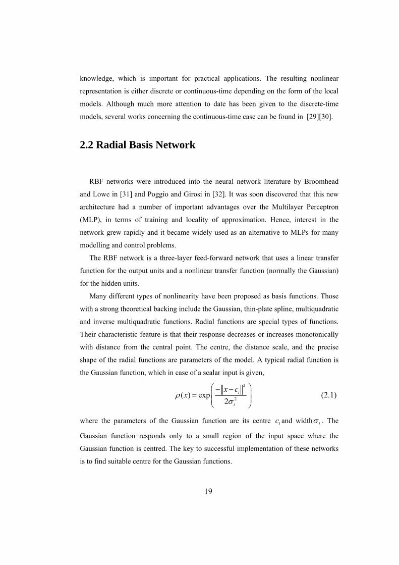
Many different types of nonlinearity have been proposed as basis functions. Those
with a strong theoretical backing include the Gaussian, thin-plate spline, multiquadratic
and inverse multiquadratic functions. Radial functions are special types of functions.
Their characteristic feature is that their response decreases or increases monotonically
with distance from the central point. The centre, the distance scale, and the precise
shape of the radial functions are parameters of the model. A typical radial function is
the Gaussian function, which in case of a scalar input is given,
2
2( ) exp
2i
i
x cx
(2.1)
where the parameters of the Gaussian function are its centre ic and width i . The
Gaussian function responds only to a small region of the input space where the
Gaussian function is centred. The key to successful implementation of these networks
is to find suitable centre for the Gaussian functions.
20
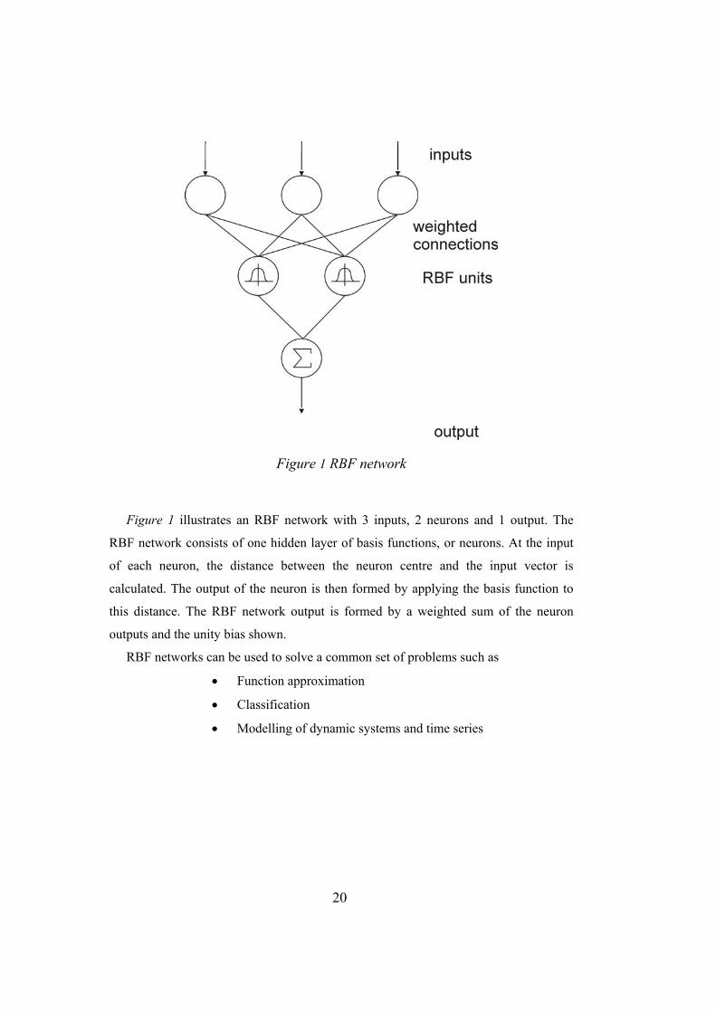
Figure 1 RBF network
Figure 1 illustrates an RBF network with 3 inputs, 2 neurons and 1 output. The
RBF network consists of one hidden layer of basis functions, or neurons. At the input
of each neuron, the distance between the neuron centre and the input vector is
calculated. The output of the neuron is then formed by applying the basis function to
this distance. The RBF network output is formed by a weighted sum of the neuron
outputs and the unity bias shown.
RBF networks can be used to solve a common set of problems such as
Function approximation
Classification
Modelling of dynamic systems and time series

21
2.3 RBF-ARX Model
In model based control strategies for nonlinear systems, RBF networks provide a
framework for modelling the system to be controlled. However, in many real
applications many RBF centres are needed for required precision which leads to the
problems in parameter estimation. State-dependent AutoRegresive model with
eXogenous variable (ARX) can be often used for modelling complex nonlinear
systems. Connection of ARX models with the RBF network has the advantages of both
the state-dependent ARX models for description of dynamics of the system and the
RBF networks in function approximation. In general RBF-ARX network uses far fewer
RBF centres when compared with a standard RBF network model.
The nonlinear system can be described by the following nonlinear ARX model
( ) ( ( 1)) ( )
( 1) [ ( 1),.... ( ), ( 1),... ( )]a b
y k f k e k
k y k y k n u k u k n
φ
φ (2.2)
where ( )y k is the output, ( )u k is the input, e(k) is the white noise and ( 1)k φ is a
regression vector. Various kinds of function can be used to approximate the nonlinear
function (.)f . A general version is the state-dependent ARX model.
0 , ,1 1
( ) ( ( 1)) ( ( 1)) ( ) ( ( 1)) ( ) ( )a bn n
y i u ii i
y k k k y k i k u k i e k
φ φ φ (2.3)
where 0 , ,, ,y i u i are the coefficients which depend on the vector ( 1)k φ . Here,
( 1)k φ is regarded as vector of past input and output values at the step k, but in many
cases ( 1)k φ can be only output signal, input signal or any other measured signal.
The basic idea of the state-dependent ARX model is to provide the local linearization
of the general NARX model. The RBF network can be used to approximate the state-
dependent coefficient because it can approximate any function. The model derived is
called the RBF-ARX model and can be defined by
22
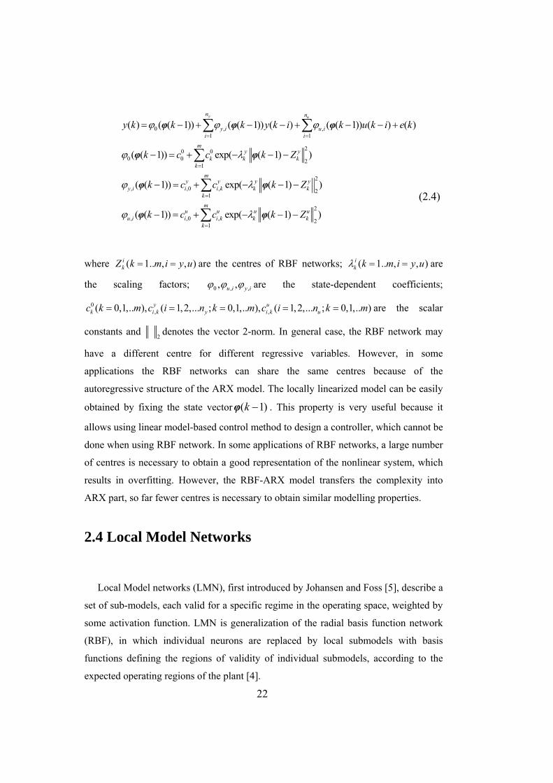
0 , ,1 1
20 00 0 2
1
2
, ,0 , 21
, ,0 ,
( ) ( ( 1)) ( ( 1)) ( ) ( ( 1)) ( ) ( )
( ( 1)) exp( ( 1) )
( ( 1)) exp( ( 1) )
( ( 1)) exp( (
y un n
y i u ii i
my y
k k kk
my y y y
y i i i k k kk
u u uu i i i k k
y k k k y k i k u k i e k
k c c k Z
k c c k Z
k c c k
φ φ φ
φ φ
φ φ
φ φ2
21
1) )m
uk
k
Z
(2.4)
where ( 1.. , , )ikZ k m i y u are the centres of RBF networks; ( 1.. , , )i
k k m i y u are
the scaling factors; 0 , ,, ,u i y i are the state-dependent coefficients;
0, ,( 0,1,.. ), ( 1,2,... ; 0,1,.. ), ( 1,2,... ; 0,1,.. )y u
k i k y i k uc k m c i n k m c i n k m are the scalar
constants and 2
denotes the vector 2-norm. In general case, the RBF network may
have a different centre for different regressive variables. However, in some
applications the RBF networks can share the same centres because of the
autoregressive structure of the ARX model. The locally linearized model can be easily
obtained by fixing the state vector ( 1)k φ . This property is very useful because it
allows using linear model-based control method to design a controller, which cannot be
done when using RBF network. In some applications of RBF networks, a large number
of centres is necessary to obtain a good representation of the nonlinear system, which
results in overfitting. However, the RBF-ARX model transfers the complexity into
ARX part, so far fewer centres is necessary to obtain similar modelling properties.
2.4 Local Model Networks
Local Model networks (LMN), first introduced by Johansen and Foss [5], describe a
set of sub-models, each valid for a specific regime in the operating space, weighted by
some activation function. LMN is generalization of the radial basis function network
(RBF), in which individual neurons are replaced by local submodels with basis
functions defining the regions of validity of individual submodels, according to the
expected operating regions of the plant [4].
23
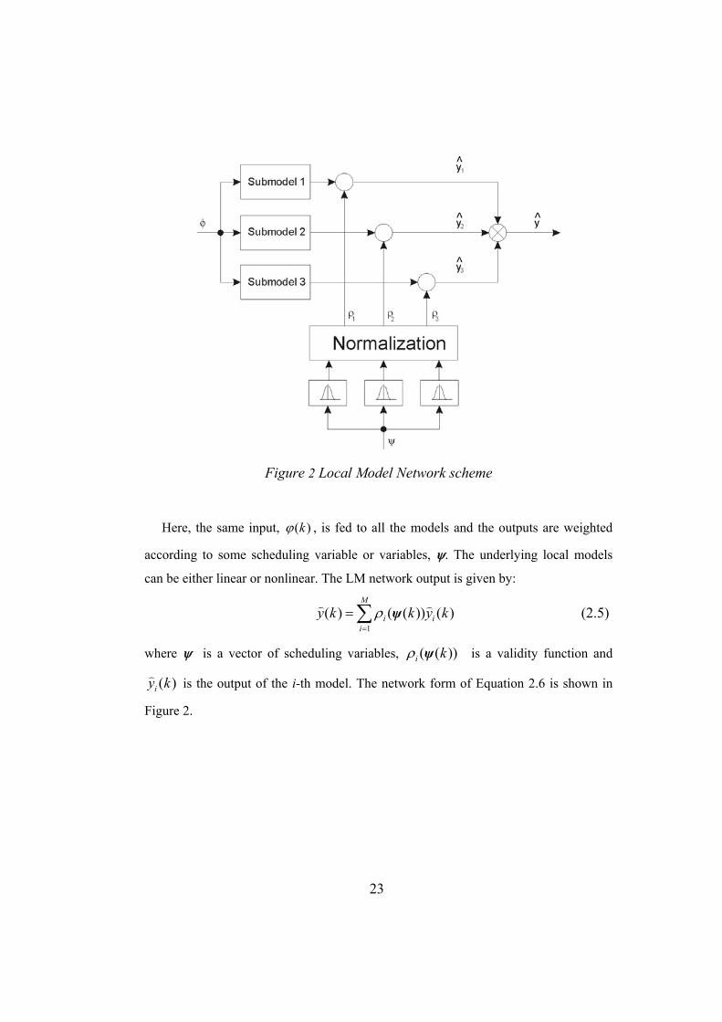
Figure 2 Local Model Network scheme
Here, the same input, ( )k , is fed to all the models and the outputs are weighted
according to some scheduling variable or variables, . The underlying local models
can be either linear or nonlinear. The LM network output is given by:
1
( ) ( ( )) ( )M
i ii
y k k y k
ψ
(2.5)
where is a vector of scheduling variables, ( ( ))i k ψ is a validity function and
( )iy k
is the output of the i-th model. The network form of Equation 2.6 is shown in
Figure 2.

24
Figure 3 The nonlinear input/output approximation (c) is obtained by combining three
linear models (a) with validity functions (b)
The modelling performance of the LMN is depicted in Figure 3, where three local
models are combined with three two-dimensional validity functions to produce
nonlinear approximation. The assumption for the local modelling approach is that the
modelled plant has to undergo significant changes in operating conditions as it moves
in the operating space. Introducing the simpler models can reduce the complexity of
the nonlinear system. For example, local state-space and ARMAX models can be
formed using localised perturbation signals and then blended to produce global
nonlinear state-space and NARMAX (nonlinear ARMAX) representations.
25
2.5 Validity functions
The blending of local models is calculated using the weighting or validity functions.
Although any function with locally limited activation might be applied as a validity
function, a common choice for this function takes the form of Gaussian. Other popular
validity functions as B-splines or multiquadratic functions have been proposed.
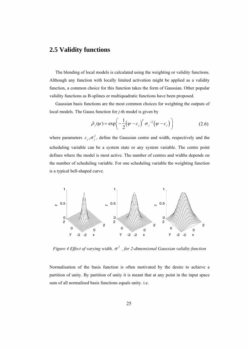
Gaussian basis functions are the most common choices for weighting the outputs of
local models. The Gauss function for j-th model is given by
21( ) exp
2
T
j j j jc c
(2.6)
where parameters 2,j jc , define the Gaussian centre and width, respectively and the
scheduling variable can be a system state or any system variable. The centre point
defines where the model is most active. The number of centres and widths depends on
the number of scheduling variable. For one scheduling variable the weighting function
is a typical bell-shaped curve.
Figure 4 Effect of varying width, 2 , for 2-dimensional Gaussian validity function
Normalisation of the basis function is often motivated by the desire to achieve a
partition of unity. By partition of unity it is meant that at any point in the input space
sum of all normalised basis functions equals unity. i.e.

26
1
( ) 1M
jj
ψ (2.7)
Validity function represents the partition of the input space in the local model network
structure. The normalised form of the validity function is denoted by ( )j ψ , for the
basis functions associated with local model j
1
( )( )
( )
jj M
jj
(2.8)
However, normalization also leads to a number of other important side-effects that
have consequences for the resulting network [33].
2.6 Side-effects of the normalization of validity functions
The normalized validity functions are often homogenous validity functions with
different parameters. Once normalized, the shape of the validity function usually
differs from the un-normalized basis function. The shape of the validity function is not
only influenced by its width but also by the proximity of other validity functions. It can
be seen from Equation 2.9 that each validity function is a function of all the original
validity functions. Therefore, a change in the parameters of one validity function
influences all other normalized validity functions. Other problem connected with the
normalization of validity function is reactivation and shift in maxima. If centres are not
uniformly distributed or the validity functions differ in widths, the maximum of the
basis function may no longer be at its centre. Furthermore, the validity function can
become multi-modal, i.e. it increases as the distance from the original centre increases,
instead of continuously decreasing.

27
Figure 5 Reactivation of the validity functions for scalar scheduling variable x
In general, assuming monotonically decreasing basis functions, the reactivation
point is the point at which the distance metric for the first basis function, d1, is no
longer smaller than that of the nearest basis function, d2. For the i-th Gaussian function,
the distance metric is given by:
2
i ii
cd
(2.9)
For two neighbouring Gaussian validity functions, the condition for reactivation can be
stated as:
12
1 2
c
c
(2.10)
This condition can be regarded as constraint for choosing the centres and widths of
the validity functions. Alternatively, to ensure that there will be no reactivation,
uniformly wide basis should be used.
B-splines are an alternative choice for the validity functions. The advantage of B-
splines over the Gauss functions is their inherent normalization. Therefore, there are no
side-effects associated with the normalization. Unfortunately, B-splines are subject to
curse of dimensionality, limiting their usefulness for low dimensional problems.

28
2.7 Local Models
The dynamics of an individual model is of particular interest as it provides basis for
the design of local controllers. One of the advantages with local modelling is that the
structure of the local models does not need to be very complex. Usually simple linear
models are sufficient. However, the local models f in Equation (2.2) can be of any
form; they can be linear or nonlinear; have state-space or input-output description, or
be discrete or continuous-time. The models can be even of different character, i.e.
parametric models for operation conditions where description is available a priori and
neural network where there is lack of physical description. However, this
heterogenous LM network would require different optimization techniques and
therefore the same type of local models throughout the LMN structure is used.
There is an obvious trade-off between the number of operating regimes and
complexity of the local model. If there were only one model for the entire operating
space, it would be very complex and it would be the global model. On the other hand,
if the operating space were decomposed into numerous small operating regions, the
complexity of the local models would be much smaller. If the local model were
described only by a constant, LMN structure would be identical to RBF network. The
discrete-time nonlinear system is considered to have the general form
( ) ( ( 1),.. ( ), ( 1).... ( ), ( 1).... ( )) ( )y u ey k f y k y k n u k d u k d n e k d e k d n e k
(2.11)
Here, ( )y k is the system output, ( )u k is the input, ( )e k is a zero-mean disturbance
term and d represents the time-delay. This type of model is known as the NARMAX
(Nonlinear ARMAX) model and has been studied widely in nonlinear system
identification. If we define the data vector as
( 1) [ ( 1),...., ( ), ( 1),... ( ), ( 1),..., ( )]Ta b ck y k y k n u k u k n e k e k n φ (2.12)
then the system can be rewritten as
( ) ( 1) ( )Ty k k e k θ φ (2.13)
where the T denotes the transpose operator and θ is a vector of parameters defined as
29
1 1 1,..., , ,..., , ,...,a b c
T
n n na a b b c c θ (2.14)
The aim in empirical modelling is to find a parameterized structure which emulates
the nonlinear function f.
Using the Equations (2.13) and (2.14) the linear system can be written in the form
1 1
1 1
( ) ( )( ) ( ) ( )
( ) ( )
B z C zy k u k e k
A z A z
(2.15)
Here, the 1z is a unit delay operator and the polynomial A, B, C are
1 11
1 11
1 11
( ) 1 ....
( ) 1 ....
( ) 1 ....
nana
nbnb
ncnc
A z a z a z
B z b z b z
C z c z c z
(2.16)
An obvious benefit of using local linear models is that their parameters can be
identified using standard optimization techniques, once the weighting functions have
been defined. Rather than globally learning the local model parameters, it is sometimes
better to train each local model individually using locally-weighted, least-squares
regression and employing only the training data local to the model.
2.8 Affine modelling
Mathematically, off-equilibrium linearization leads to local affine models, which
have an extra degree of freedom. i.e., the bias term to make the models more flexible,
so they can be shifted upwards and downwards in the operating space. The bias term
can significantly improve the modelling accuracy of the LLM. However, due to the
bias term the affine models do not possess the superposition property fundamental to
the linear systems. Thus, there is a lack of continuity with established linear theory.
The inhomogeneous term can become large and significantly influnce the solution,
while the change of parameters A and B only have minor influence on the local model
accuracy. Therefore, the bias cannot be simply regarded as a small approximation error
or disturbance. With local linear models , one can achieve accurate approximation of
either the linearized dynamics or the trend, but not both simultaneously. With the
30
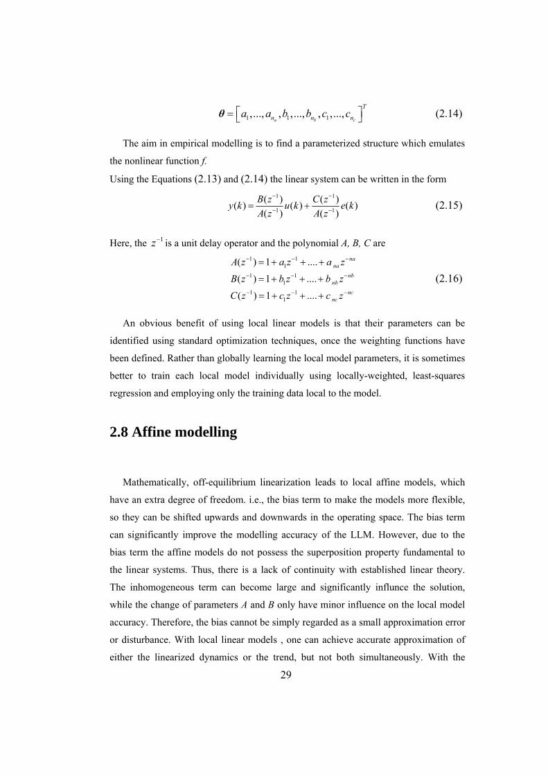
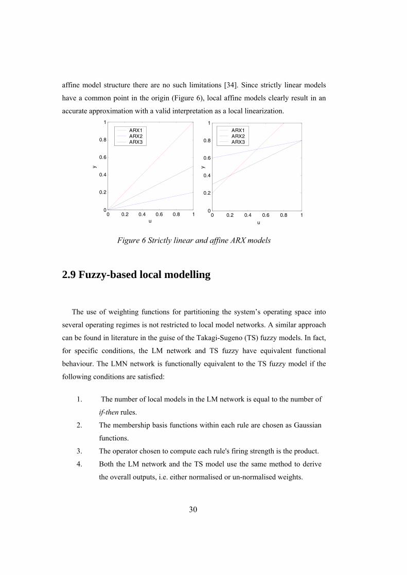
affine model structure there are no such limitations [34]. Since strictly linear models
have a common point in the origin (Figure 6), local affine models clearly result in an
accurate approximation with a valid interpretation as a local linearization.
0 0.2 0.4 0.6 0.8 10
0.2
0.4
0.6
0.8
1
u
y
ARX1ARX2ARX3
0 0.2 0.4 0.6 0.8 10
0.2
0.4
0.6
0.8
1
ARX1ARX2ARX3
y
u
Figure 6 Strictly linear and affine ARX models
2.9 Fuzzy-based local modelling
The use of weighting functions for partitioning the system’s operating space into
several operating regimes is not restricted to local model networks. A similar approach
can be found in literature in the guise of the Takagi-Sugeno (TS) fuzzy models. In fact,
for specific conditions, the LM network and TS fuzzy have equivalent functional
behaviour. The LMN network is functionally equivalent to the TS fuzzy model if the
following conditions are satisfied:
1. The number of local models in the LM network is equal to the number of
if-then rules.
2. The membership basis functions within each rule are chosen as Gaussian
functions.
3. The operator chosen to compute each rule's firing strength is the product.
4. Both the LM network and the TS model use the same method to derive
the overall outputs, i.e. either normalised or un-normalised weights.

31
2.10 Concluding remarks
The main features of the local model network have been described in this chapter. It
has been shown that LMN can be viewed as generalization of the Radial Basis
Function network where output constants at each neuron are replaced by a local model.
In the research literature the local models are often linear and the validity functions
take form of Gaussian basis function. To provide partition of unity the validity function
are normalized which can cause side-effects such as shift in maxima or loss of local
support. These side effects degrade the transparency and interpretability of the
network. These side-effects can be avoided by using B-splines, however due to the
curse of dimensionality; they are limited to the low dimensional problems. The link
between the LM network and the fuzzy-based Takagi-Sugeno model has been also
shortly outlined in this chapter. Under certain conditions, the two global models are
functionally equivalent. Thus, research analysis for both nonlinear representations is
interchangeable. The advantage of the LMNs is that it does not suffer from the
“stability-plasticity dilemma” which is a common design problem with adaptive
control where the algorithm is adapting to the new operating region, it is also forgetting
the previous regions.

32
Chapter 3 NONLINEAR
SYSTEM MODELLING USING
LOCAL MODEL NETWORKS
Modelling nonlinear dynamic systems from the observed data and prior knowledge
is an important area of science and engineering. Training is a key issue in the
application of the Local Model Networks because there is the added complexity of
having to determine the number and the structure of sub-models as well as the
parameters of the validity functions in addition to parameter identification,. There are
several methods for modelling a nonlinear system and the choice of a particular
modelling method depends on the aim of modelling. If the aim of modelling is control
design then the identification technique should lead to simple, transparent and
mathematically tractable models. In many applications it is necessary to combine the
information obtained from the numerical data with heuristic knowledge. Another major
requirement for nonlinear system modelling algorithm is the universality in the sense
that a wide class of structurally different systems can be described. The described
architecture of local model networks is capable of fulfilling these requirements and can
be applied to tasks where high degree of flexibility is required. Construction of models
of such structure involves a linear estimation of the regression models and nonlinear
optimization of the parameters of the validity functions. A general approach to
parameter estimation is to minimize some criterion that measures the difference
between the output of the model and the observation data. This is called global
learning. If the parameters of each model are identified separately using the weighted
subset of data the approach is called local modelling.

33
3.1 Divide and Conquer Strategy
Divide and Conquer approaches have drawn attention in recent years in the area of
controlling nonlinear plants over a wide range of the operating conditions. These
approaches decompose the complex nonlinear problem in a number of simpler
problems, each associated with restricted operating region. This results in transparent
representation of the control system with the opportunity to use the conventional linear
control design techniques. The Divide-and-Conquer strategies can be divided into two
groups: analytical approaches and the learning approaches. While the first one requires
the analytical form of description of the system to be controlled, the latter is based on
the input-output observations data.
Analytical approaches
- Linearization
- Gain scheduling
- Feedback linearization
Learning approaches
- Modular architecture
- Local learning
When no analytical model is available but the assumption of linearity is reasonable,
linear system identification methods are used to estimate the system’s parameters.
Linear techniques have been also employed for the nonlinear systems using the
adaptive algorithms. Here the on-line identification algorithm provides the linear
approximation of the nonlinear system in order to track variations in the dynamics. The
idea of learning techniques is to approximate the unknown relation between state of the
system and control actions by using nonlinear optimization techniques. The divide-
and-conquer idea has taken two different forms: the global learning and the local
learning. Although the global learning uses a combination of local models, their
identification is still performed on the basis of the whole dataset. Although the
simplification can be made by using the local linear models, the problem is still
nonlinear and requires the same procedures used for generic global models.

34
Figure 7 The operating range of complex systems is decomposed
into a number of operating regimes (the axis represent two scheduling variables)
3.2 The modelling process
The divide-and-conquer strategy helps to improve the techniques for the design of
models of nonlinear systems with the aid of computationally data-driven techniques.
The modelling process involves integrating the knowledge about the system with the
experimental data. The typical sources of information of the system could be:
Experimental data, such as responses to perturbations
A possibly incomplete nonlinear model that may be too simple or too
complicated
Qualitative knowledge, i.e. behaviours or engineer’s heuristics

35
The model can only represent certain aspects of the system, so it is necessary to know
the purpose of the model in order to decide which aspects should model capture.
Figure 8 Engineering approach to model development
The abstract modelling cycle (Figure 8), which covers a number of further tasks
that are essential in modelling:
Experiment design and data acquisition
Raw data processing and analysis
Analysis of a priori knowledge. Physical laws and available models
Structure and parameter optimization
Model reduction and simplification
Model validation, analysis and interpretation
36
The experimental data is used for the parameter and structure identification so it is
necessary that the data covers the important aspects of the system. The input signal
should exhibit enough amplitude and appropriate frequency range in order to excite all
interesting modes of the plant, however these requirements are often in disagreement
with the industrial practice. Once the experiments are designed, the actual input and
output sequences have to be collected. In many processes it is important to have
accurate models in stable areas than less accurate models throughout the whole
operating range, as the system usually spends most of the time in the stable area. It is
also necessary to have appropriate amount of identification data in the regions where
the system is most complex or the control is most critical. Lack of data from a certain
operating region can explain why the related local model parameters are not accurately
identified. As it can be seen, the choice of appropriate data for structure and parameter
identification is a crucial part of the modelling and requires more consideration then
subsequent machine learning [34].
3.3 Structural identification
Although a priori knowledge is important to define the model structure, in some
cases the system complexity is not well understood for the model structure to be
specified in advance. So it is often necessary to adapt the structure based on the
information in the training data. Optimization of the model structure M is, however, a
difficult non-convex optimization problem. The goal of the structure identification
procedure is to relate the density and the size of operating regimes to the complexity of
the system. The desirable features of the identification algorithm:
Convergence – as the number of training points increases the algorithm should
provide more accurate model of the system being modelled
Parsimony – the model structure should be the simplest possible to achieve the
required accuracy
Robustness – the model structure produced should be robust to the noisy data

37
Interpretability – the model structure should be as interpretable as possible
given the local models, their validity functions and available data
The techniques for the optimization of positions and dimensions of the local regions
fall into several classes:
Fixed Selection
In this approach the centres are selected randomly from the input data or
distributed uniformly [36]. The widths of operating regions are calculated to
some thumb rules based on a priori information. If the complexity of the
problem is unknown a large number model is necessary for fine approximation
of the nonlinear system. This is a rather bad clustering solution because even a
small region can be highly nonlinear.
Self-organizing and clustering
In this approach the centres of the operating regimes are trained in an
unsupervised learning fashion. Abonyi et al, in [38] and [39] used Expectation
Maximization algorithm (EM) to identify simultaneously and directly the
operating regimes and the parameters of the local models. The disadvantage
of these algorithms is that the local models are clustered according to the
density of the data, not according to the complexity of the problem.
Non-optimal construction algorithms with heuristic growing strategies
These techniques start with a simple structure, e.g. a global linear model,
and divide the input space into smaller areas. Examples are local linear model
tree (LOLIMOT) [10], Johansen and Foss algorithm [5], algorithm of Aarhus
[40] that is trying to find a split point in which to carry out the decomposition
of the input space to reduce the prediction error. Kavli in [41] developed an
ASMOD algorithm that uses B-Splines to represent general nonlinear and
coupled dependencies in multivariable observation data. Jakubek and Kreuth
[42] created an iterative construction algorithm that tries to fit the local models
to the available data using statistical criteria along with regularization.

38
Splitting and merging
These algorithms try to adjust the network complexity according to the
complexity of the problem. The algorithm splits an operating region into two,
if the behaviour of the model is not satisfactory and two neighboring models
are merged together if they have nearly identical parameters to limit the
complexity of network.
Fine-to-course learning
These techniques start with a large number of local models and during training
the local model are merged together to get a simple structure [43].
While the comparison between the algorithms of Johansen and Foss and Nelles can
be found in [44], the work by McGinnity and Irwin [45] compares the hybrid
optimization algorithm by McLoone and Johansen and Foss algorithm.
All the structure identification algorithms are computationally expensive. This
problem becomes crucial if a number of models or input dimension of the network
becomes large. Therefore, it is always advantageous to consider the maximum possible
a priori information about the system.
3.4 Heuristic strategies for structure identification
The following part addresses the problem of identifying a model of an unknown
non-linear system on the basis of a sequence of N input/output pairs
( (1), (1)),........, ( ( ), ( ))N u y u N y ND (3.1)
where ( ), ( )y k u k are the system outputs and input respectively. A global model can be
formed
1
( ) ( , ) ( )M
ii
y f
ψ θ φ ψ
(3.2)
where ψ is the vector of scheduling variables. The addressed problem is estimation of
this function, since the function immediately gives the model equations. The model
structure based on modular description of N regimes can be written
39
, ,N i i iM Z f
(3.3)
where regime Zi represents subspace of the whole operating space. The modelling
problem consists of the following sub-problems:
1. Choose the variables which to characterize the operating regimes with
2. Decompose Operating space Z into regimes and choose local model structure
3. Identify the local model parameters for all the models
An appropriate order for the identified model may be determined by the Akaike
information criterion (AIC) [46]. The procedure is to repeat the identification process
for different orders and choose the final model by looking for a small AIC value,
together with appropriate model dynamics.
The AIC is defined as
log 1 2d
AIC JN
(3.4)
where d is a total number of estimated parameters, N is the length of the data record
and J is the loss function for the structure in question.
3.4.1 Johansen and Foss Algorithm
For modelling the nonlinear process the J&F algorithm [5], which incorporates an
outer loop for structure optimization and inner loop for parameter identification, can be
used. The scheduling variables have to be known beforehand. The J&F algorithm starts
with only one model and the weighting function is unity over the whole operating d-
dimensional space Z, where d is the number of scheduling variables. Using the least-
squares method, the parameters estimation of the only model can be performed. The
algorithm then divides the operating space into two parts (Figure 9). Since an infinite
number of divisions is possible it is necessary to reduce the number of divisions being
investigated. This is done by only allowing the regime to be divided in a direction
parallel to an axis of the box Z1 which defines an operating regime, and at a finite
number of points along each axis.

40
Figure 9 Operating regime decomposition
Thus for a d-dimensional box with s splitting points, a total of ds new
decompositions are formed. New parameters of weighting functions are determined by
the limits of each working regime
max min
max min
0.5( )
0.5 ( )
j j j
j j j
c z z
z z
(3.5)
where parameter influences the overlapping of Gauss function and maxjz , min
jz are
limits of the j-th regime. For small values of the functions will not overlap and for
large values the transition from one region to another will be smooth. Once the
weighting functions parameters are obtained, the parameters of the local models can be
estimated by least-squares method (Chapter 3.7) or weighted least-squares method
(Chapter 3.8).
For each split the value of cost function is calculated and the parameters of local
models are determined. After considering all possible splits, the one with the lowest
cost function is then chosen and the procedure is repeated. This process continues until
either a maximum number, M, of regimes is found or until some pre-specified

41
modelling cost criterion is satisfied. The construction algorithms can also effectively
determine which variables are required to suitably decompose the operating space. If
no splits are formed over a particular axis, then the variable associated with that axis
can be ignored.
3.4.2 LOLIMOT algorithm
This method splits up the identification procedure into two parts. In the outer loop,
the structure of the local model network is optimized by a tree construction algorithm.
In a inner loop the parameters of the local models are estimated by local modelling
technique. The construction algorithm partitions the input space by orthonormal cuts
dividing the worst performance local model along the input axis, which yields the
highest improvement [10]. Consequently, the nonlinear model complexity
automatically adapts to the complexity of the process.
At first sight, both algorithms appear to be very similar. However, there is an
obvious trade-off between computation complexity and model optimality. While the
J&F technique tries to achieve an optimal model at the expense of intensive
computation, LOLIMOT minimizes the computational effort involved at the risk of
producing a sub-optimal model. In general, the J&F algorithm produces a more
accurate representation than LOLIMOT but with a considerable increase in
computational effort required. Comparison on the computational costs and modelling
performances of both techniques can be found in [44].
3.5 Structure optimization via the SOMA algorithm
Self-Organizing Migration algorithm (SOMA) [48] is a genetic algorithm that is
based on the competitive-cooperative behaviour of intelligent creatures solving a
common problem. Such behaviour of intelligent creatures can be observed anywhere in
the real world. A group of wolves or other predators may be a good example. If they

42
are looking for food, they usually cooperate and compete so that if one member of the
group is more successful than the previous best one (e.g. has found more food) then all
members change their trajectories towards the new most successful member. The
procedure is repeated until all members meet at one food source. In SOMA, wolves are
replaced by individuals. They ‘live’ in the optimized model’s hyperspace, looking for
the best solution. This kind of behaviour of intelligent individuals allows SOMA to
realize very successful searches.
Because SOMA uses the philosophy of competition and cooperation, the variants of
SOMA are called strategies. They differ in the way the individuals affect all others.
The basic strategy is called 'AllToOne'. Before starting the algorithm, the SOMA
parameters such as population size or number and migrations has to be defined. The
user must also create the specimen and the cost function that will be optimized. Cost
function is a wrapper for the real model and must return a scalar value, which is used
as gauge of the position fitness.
SOMA, as well as the other evolutionary algorithms, works on a population of
individuals. Each individual represents an actual solution of the given problem. In fact,
it is a set of parameters for the cost function, whose optimal setting is being searched.
The cost function response (cost value) to the input parameters is associated with each
individual. The cost value represents the fitness of the evaluated individual. It does not
take part in the evolutionary process itself; it only guides the search process.
For LMN optimization with local ARX models an individual that represents
possible solution of the optimization problem have the following structure:
Figure 10 Individual representing possible solution of the optimization problem
Usage of all the model parameters for optimization leads to the same problems as in
the global learning technique since each local model influences all the other models.
Possible solution is combination of SOMA optimization algorithm for optimization of
43
the validity function parameters combined with the least-squared method for local
model parameters estimation.
In the SOMA optimization process it is easy to penalize the LMNs with unstable
local models or with the reactivation of the validity function by simply adding a
constant to the value of modelling criterion to prevent these LMNs to create possible
global optimum of the optimization problem.
3.6 Parameter Estimation in Local Model Network
Structure
The problem of parameter estimation for systems which are linear in parameters is
reasonably well understood, with variety of efficient optimization techniques to
optimize the parameters θ of the local models. Parameter optimization for a given
model structure finds the optimal costs
*( , ) min ( , , )J JM D θ M D (3.1)
where M is a given structure of the network 1( , , ... )MnM MM c σ (i.e. centers
and widths of the validity functions and local models structure) and D is the
training data set ( ( 1), ( ), 1.. )k y k k N D .
3.7 Global learning
If we assume models linear in parameters and fixed parameters of validity function,
the learning problem is the application of the least-squares method to obtain the
parameters θ
. Using the matrix form we obtain the following regression model
T y θ Φ ε (3.2)
where the matrix Φ contains the rows defined by the term

44
1( ( )) ( ),....., ( ( )) ( )k Mk k k k Φ ψ φ ψ φ (3.3)
where ( )kφ is a regression data vector. In Equation (3.3) the values of the validity
functions are fixed either for one individual of the SOMA algorithm or one possible
division point of the Johansen and Foss algorithm.
Matrix Φ , regression vector ( )kφ , output data vector y , error vector ε and
parameters vector θ
are defined as follows:
1
1
1
1
1 1
( ) ( 1),..., ( ), ( 1),..., ( )
,....,
,....,
[ , , ]
,..., , ,...,
N
N
N
TM
Tj j j jj na nb
k y k y k na u k u k nb
y y
a a b b
Φ
Φ
Φ
φ
y
ε
θ θ θ
θ
(3.4)
Criterion for the least squares estimation is given by
1
( )TT TJ
N θ y θ Φ y θ Φ
(3.5)
where N stands for the size of measured data and parameter estimates can be obtained
using the equation
1( )T T θ Φ y Φ Φ Φ y
(3.6)
where Moore-Penroseho pseudoinverse +Φ [35], can be calculated using the singular
decomposition. Using the singular decomposition the matrix Φ can be divided into
terms so that:
T
T
+ +
Φ USV
Φ = VS U (3.7)
The numerical algorithm for the calculation of the pseudoinverse is called Singular
Value Decomposition SVD. Once the singular values have been zeroed, the parameters
of the local models can be computed.
T +θ VS U y
(3.8)

45
3.8 Local Learning
Global learning is based on the assumption that parameters of all the local models
are estimated in one step. In general, the global learning is more accurate than local
learning. In Murray-Smith and Johansen [4] showed that global learning does not
guarantee to produce local models that will be close approximation to local
linearization of the system. Global learning can also become computationally if a large
number of models or data are used. The other choice which does not posses the
aforementioned disadvantages is to estimate independently parameters of each model.
Parameters of the local models are estimated using the weighted criterion for i-th
model
1
( )TT T
j j j j jJN θ y θ Ω Q y θ Ω
(3.9)
where 1,...j M . jQ is an N x N diagonal weight matrix, where diagonal elements
of the matrix are used to weight the importance of the different samples in the training
set on i-th local model. The matrix of measured data Ω is defined as
(1)
.
.
( )N
φ
Ω
φ
(3.10)
The importance of the samples to j-th model is given directly by the unnormalized
individual validity function that are fixed either for one individual of the SOMA
algorithm or one possible division point of the Johansen and Foss algorithm.
( ( (1)),..., ( ( )))j j jdiag N Q ψ ψ (3.11)
Parameters ,jθ y
in the Equation (3.9) remain the same as in the previous chapter. The
locally weighted estimates of parameters of a local model jθ
are given by minimum
of the criterion jJ .
1T Tj j j
θ Ω Q Ω Ω Q y
(3.12)

46
3.9 Incorporating a priori knowledge
A major advantage of the local model networks is that they are not only useful
architectures for general learning tasks, but that it is relatively easy to introduce the a
priori knowledge about a particular problem. A priori information is initial knowledge
about the system or a problem in question. As can be seen from Figure 8 a priori
knowledge plays an important role at each stage of the modelling process. A priori
knowledge includes goals of the problem, characteristics of the system, its parameters
and effect of the environment (disturbances and noise). The most general form of
information is the expected dynamic order of the models, the form of the models (e.g.
ARX models) and the sampling period. In many cases, there will not be sufficient data
to train the model throughout the input space, especially outside the areas of normal
operation. This can be overcome by fixing a priori models to the areas where system is
well understood and applying the learning techniques only where data is available and
reliable. A further option, for cases where a complex and too complicated model exists
and is valid for certain operating regimes, is to pre-set the fixed local models obtained
through the linearization of the nonlinear model. The linearization of the nonlinear
model can also be used for comparison with the model obtained from the experimental
data.
The problem of choosing the local model dynamic order and the sampling period is
not a simple task. The problem of order selection and sampling period is widely
discussed in the identification literature [49].
Determining model parameters from a finite set of observation is an ill-posed
problem, since a unique model may not exist or it my not depend on the observations.
Even if the data are not corrupted by noise, the model can exhibit random behaviour at
an operating point that is not exactly captured by the observation data set. It is often
desirable to employ all the available prior knowledge and observation data to obtain a
better conditioned problem. This will generally lead to a better model. The available
prior knowledge used through optimization can have several forms: smoothness of the
model behaviour, partially or completely known local models, constraints on the
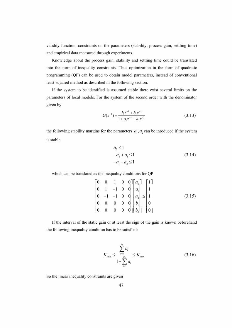
47
validity function, constraints on the parameters (stability, process gain, settling time)
and empirical data measured through experiments.
Knowledge about the process gain, stability and settling time could be translated
into the form of inequality constraints. Thus optimization in the form of quadratic
programming (QP) can be used to obtain model parameters, instead of conventional
least-squared method as described in the following section.
If the system to be identified is assumed stable there exist several limits on the
parameters of local models. For the system of the second order with the denominator
given by
1 1
1 1 21 2
1 2
( )1
b z b zG z
a z a z
(3.13)
the following stability margins for the parameters 1 2,a a can be inroduced if the system
is stable
2
2 1
1 2
1
1
1
a
a a
a a
(3.14)
which can be translated as the inequality conditions for QP
0
1
2
1
2
0 0 1 0 0 1
0 1 1 0 0 1
0 1 1 0 0 1
0 0 0 0 0 0
0 0 0 0 0 0
a
a
a
b
b
(3.15)
If the interval of the static gain or at least the sign of the gain is known beforehand
the following inequality condition has to be satisfied:
1min max
1
1
b
a
n
ii
n
ii
bK K
a
(3.16)
So the linear inequality constraints are given

48
min
1 1
max1 1
1 0,
1 0
a b
a b
n n
i ii i
n n
i ii i
K a b
K a b
(3.17)
If the global modelling approach is employed in the training algorithm and
following regression model is used
T y Φ θ ε (3.18)
with affine ARX models of the second-order, the regression matrix and vector of
outputs are defined:
(3)
(4)
:
( )
y
y
y N
y (3.19)
1( ( )) ( ),....., ( ( )) ( )Tk Mk k k k Φ ψ φ ψ φ (3.20)
The least-squares method can be solved by
1( )T Tθ Φ Φ Φ y
(3.21)
The constrained optimization problem can be formulated as:
1
min2
T T θ
θ Hθ c θ
(3.22)
with
2 , 2T T H Φ Φ c Φ y (3.23)
and the constraints
inq A θ b
(3.24)
By using the constraints during the training process, more accurate model with
improved interpretability can be identified using the input-output data [50].

49
3.10 Validation
Practically it is impossible to develop a model that would completely describe the
true system. There will be always some features in the true system, which the model
cannot describe. At this stage the quality of the mode is evaluated by analyzing how
well it captures the data. Usually, validation is performed by combination of statistical
measures that evaluate the generalization capability of the mode, and qualitative
criteria, focus on establishing how the model relates to a priori knowledge, how it easy
to be used and interpreted. In literature there are several methods for model validation,
see [49] for a thorough discussion. The most common technique is to compare the
predictions generated by the model with the measured data.
When validating a model a cross validation method is often used. This means that a
model is validated using new data. For this purpose the data set is divided into two
parts where one set is used for identification purposes and one for validation.
3.11 Concluding Remarks
At the beginning of the chapter the basics of divide-and-conquer strategy and
identification from experimental data are given. An important aspect when creating a
learning algorithm for local model structure is the trade-off between achieving a good
global fit and good local representation. Global learning methods are computationally
more expensive and obtained models can not be interpreted as valid linearizations of
the underlying nonlinear system because each model is influenced by all the other
models. When identifying the local models by minimizing locally weighted prediction
error criteria, the local models have locally valid interpretations as linearizations. On
the other hand, the global prediction performance is typically inferior to what can be
achieved by global optimization. Analysis and comparison of local and global learning
method can be found in [4]. A learning algorithm for a local model network has to
perform two tasks: identification of the network structure and estimation of local model
parameters. Structure identification comprises of the determination of the number and

50
distribution and shape of the operating regions and the parameters of the weighting
functions. Description of various learning techniques for training of local model
networks has been given in the previous sub-sections. Constructive techniques which
gradually increase the number of models to achieve better model representation have
several advantages. Firstly, the main features of a process are captured first, then
details. The overfitting protection of the constructive algorithm also limits overtraining.
Since the number of divisions is restricted in these algorithms, better global fit can be
achieved via optimization technique that utilizes the evolutionary algorithms. SOMA
algorithm for the construction of the local model network has been proposed. The
approach optimizes either all the local model parameters or only the parameters of the
validity functions and constraints that ensure transparency and local interpretability can
be easily integrated. The use of constraints is useful to identify interpretable local
models, especially when the assumption for excitation is not strongly satisfied. The
modelling performances of the training algorithms approaches have been evaluated
using simulated data from pH neutralization process in the experimental part of this
thesis.

51
Chapter 4 CONTROLLER
DESIGN BASED ON LOCAL
LINEAR MODEL
DESCRIPTION
The local model network control structure utilizes, in most cases, two local model
networks. One network is responsible for identification, while the other servers as a
controller. In an adaptive scheme the identification network is updated at each
sampling interval.
The multiple model controller design method is characterized by three steps
1. the plant is modelled by local model network composed of M local linear
models
2. a feedback controller is designed for each local model in order to guarantee
local stability and robustness
3. global controller is obtained by combining the local controllers via the validity
functions
This approach seems quite similar to the Gain scheduling approach but there are
two main differences:
1. In the LMN scheme the local models are not linearized about the equilibrium
points but about generic operating points
2. Unlike the Gain scheduling, the LMN approach requires no analytical
description of the system
Basically, there are two ways to design controllers for local model structures, the
linearization based and the local model-based approach. For linearization-based
approach the local model network is linearized at the current operating point and linear

52
controller is designed. The linearization of the LM network is very simple due to the
structure of the model. This approach is used for the controller design in the next
sections. In the second approach a local controller is designed for each local model and
the control output is then calculated as an interpolation of the local controller according
to the current operating point.
Figure 11 Controller design using linearization and local models (LLM – local linear
model, LLC local linear controller)
Only the SISO systems are considered within this chapter, however, extension for
the MIMO case can be easily derived for predictive controller.
4.1 Local Controller Networks
Once the LMN is constructed, local controller network, the control version of LMN
is defined in turn. In general, the global control signal is determined by
1
( ) ( ( ), ( ( )))M
ci i
i
u k C k k
φ ψ (3.25)
where iC denotes the local controller for a local model i. The local controllers are
blended using the same validity functions i , which are used in LM network. The
controller information vector cφ consists of past controller outputs, current and past
plant outputs and the current and past values of reference signal. There are two
53
different possibilities of handling the states of the controller. Either the local
controllers may share common states or each controller can have its own states.
4.2 Model Predictive Control
Model-based Predictive control is becoming widely used in industry due to its
ability to handle difficult control problems such as multi-input multi-output processes
or constraints in the system variables. Model Predictive Control (MPC) refers to a class
of algorithms that compute a sequence of manipulated variable adjustments in order to
optimize the future behaviour of the plant. Camacho and Bordons in [51] provide
practical aspects of the most commonly used MPC strategies and also an overview of
commercially available MPC technology. MPC algorithms possess common elements,
in which different options for each element give different algorithm.
Most MPC technologies are based on linear input-output models (transfer
functions, step response models). These models are usually identified from the
plant input-output data. The accuracy of the identified model is crucial for the
performance of the MPC algorithm.
At each sampling point the inputs are determined from optimization of a
quadratic performance objective over finite prediction horizon.
Future outputs are specified by set-points or reference trajectories.
Input and output constraints, which can be hard or soft, are included in the
optimization process.

54
Figure 12 The receding horizon strategy, the basic idea of predictive control
The basic idea of the model predictive control ( Figure 12) is to determine the control
action u(k) at time t =kT, by using the sampling period time T and solving a finite-
horizon optimization problem over a time interval of , ( )t kT k N T . At the
new time instant a new control u(k+1) is found by solving a new optimization
problem for the next time interval. The one-step prediction of the nonlinear
system is given
( 1) ( ),...., ( 1), ( ),...., ( 1)y uy k f y k y k n u k u k n
, (4.1)
where f
is an approximation of the nonlinear system. Moreover, the input and
output vectors
, , 1,.., , 1,..,p cy k i Y u k j U i H j H (4.2)
u(k),y(k) must lie within the boundaries given by Y and U which are compact sets mR
and rR respectively. The control is determined by minimization of the quadratic
objective function defined as
1 1
( ) ( ) ( ) ( )p c
H HT T
i j
J e k i e k i j u k j
(4.3)

55
where the vector ( ) ( ) ( )e k i w k i y k i represents the error between the desired
output and predicted output at time ( )t k i T . ,p cH H are prediction and control
horizons respectively. u is defined as an incremental
change ( ) ( ) ( 1)u k u k u k since it is the change of the input signal that is
unwanted. The coefficient is usually a constant or an exponential sequence that
penalizes the differences of future efforts. Since the predictive control strategy is based
on the receding horizon, so that at each instant the horizon is displaced towards the
future, which involves application of the first control signal of the sequence solved at
each sampling time.
Although only the first element of the vector ( ),..., ( 1)cu k u k H is used for
control, the other elements can be effectively used to initiate the optimization
procedure at the step ( 1)t k T .
4.3 Nonlinear Model Predictive Control
In general, industrial processes are nonlinear, but most MPC applications are based
on the use of linear models. The first reason is that identification of a linear model is
relatively simple and the linear models are sufficient when the plant is operating in the
neighbourhood of the operating point. Secondly, the use of linear models with
quadratic objective function gives rise to a convex problem which can be solved by
Quadratic Programming. Thus two major issues limit its application to nonlinear
systems. Firstly, the assumption for the predictive control is a quite accurate model of
the system. However, complex systems are often connected with nonlinearities, wide
operating range or uncertainty. The second is that a nonlinear non-convex
optimization problem must be solved for each sampling period with very
computationally demanding algorithms. A wide variety of models has been used for
nonlinear model predictive algorithms.
These include:
Nonlinear differential equations
Hammerstein [52], Wiener, Volterra [53]and Laguerre models [54]

56
NARMAX models
Neural networks [14],[55],[56],[57]
Fuzzy models
The local linear model structure offers several advantages in the model predictive
control scheme. The LLM network provides good prediction of the future trajectory of
the system but also the parameters of the plant at each operating point. If the local
models are of the affine ARX form
0 1 1( ) ( ) .... ( ) ( ) ... ( )i i i ii na a nb bf a a y k a y k n b u k b u k n (4.4)
then the nonlinear network is given
0 1 1( 1) ( ) ... ( ) ( ) ... ( )na a nb by k A A y k A y k n B u k B u k n (4.5)
which is an ARX model with its parameters defined at each operating point:
1 1 1 11 1
( ) , ( ) ,....M M
i ij j
j j
A a B b
(4.6)
This technique allows the use of a linear predictive controller and thus avoids the
problems associated with computation time and optimality of the nonlinear solution.
This technique can be viewed as a successive linearization around the operating point
which yields linear MPC. The local model structure enables easy linearization of the
nonlinear model due to its structure. For nonlinear systems the parameters of the
linearized model can vary from the parameters of the system along the prediction
horizon. The techniques to compute the model parameters along the prediction horizon
are described in Chapters 4.4 and 4.5.
4.4 Single-model predictions
The predictor of the linearized model for the prediction horizon Hp is given by
( ) ( ) ( )k k k y Px R Qu (4.7)
where ( )k Px R is free response of the system that depends only on the past inputs
and outputs and ( )kQu represents forced response that depends only on future inputs.

57
( ) ( 1),....., ( )T
pk y k y k H y
(4.8)
( ) ( ),..., ( 1), ( 1),...,. ( 1)T
a bk y k y k n u k u k n x (4.9)
( ) ( ),...., ( 1)ck u k u k H u (4.10)
11 1( 1)
1 ( 1)p p
na nb
H H na nb
p p
p p
P
(4.11)
11
21 22
1 2
0 ... 0
... 0
...
...p p p cH H H H
q
q q
q q q
Q (4.12)
1[ .... ]p
THr rR (4.13)
The coefficient of matrices P, Q, R for the affine second-order ARX models and
prediction horizon equal to control horizon are given
11 1 12 2 13 2
21 1 11 2 22 1 12 23 1 13
1 1 ( 1)1 2 ( 2)1 2 1 ( 1)2 2 ( 2)2
3 1 ( 1)3 2 ( 2)3
, ,
, ,
, ,
3,...,
i i i i i i
i i i p
p a p a p b
p a p a p a p p a p
p a p a p p a p a p
p a p a p for i H
(4.14)
1
( 1) 2
1 ( 1) 2 ( 2)
1,...,
1,..., 1
1.. 2...
ii c
i i c
ij i j i j c c
q b for i H
q b for i H
q a q a q for j H and for i j H
(4.15)
1 0
2 1 0 0
1 ( 1) 2 ( 2)i i i
r a
r a a a
r a r a r
(4.16)
To eliminate steady-state errors caused by the modelling mismatch between the
plant and model the estimated modelling error err(k) is computed at each sampling
step
( ) ( ) ( )err k y k y k (4.17)

58
where ( )y k
is the 1-step ahead prediction at time (k-1). The estimate of error is then
filtered to minimize the instability introduced by modelling error feedback. More
complicated observers/compensators can be implemented within the control loop to
prevent from the effect of model/plant mismatch that are responsible for static offset
[58].
The predictive control algorithm consists of applying a control sequence that
minimizes a cost function of the form
2 2
1 1
( | ) ( ) ( 1)p c
N N
j j
J y k j k w k j u k j
(4.18)
Expression (4.18) can be rewritten as
( ) ( )T TJ err err Px Qu R T w Px Qu R T w u u (4.19)
where matrix T is defined as
1
2 1
1 1 2 2
1
1
i i i
t
t a
t a t a t
(4.20)
The minimum of J, assuming there are no constraints on the control signals and 0 ,
can be found by making the gradient J equal to zero, which leads to:
1( ) [ ] [ ( ) ( ) ( )]T Tk k k err k u Q Q Q W PX R T (4.21)
where ( ) [ ( 1),..., ( )]Tpk w k w k H W is a vector of future set-points and err(k)
is an estimate of modelling error ( ) ( ) ( )e k y k y k . Equation (4.19) with omitting the parts that do not involve the future control signal u
and only shift the value of the cost function J can be rewritten as
1
2T TJ u Hu b u (4.22)
where
( ) ( )
T T
T T Terr
H Q Q M M
b Q Px w R T N M (4.23)

59
where the matrix M is defined as
0 0 0
0 00
, ( 1)0
00
0 0
u k
M N
(4.24)
If constraints are introduced the quadratic programming (QP) problem has to be solved
in every instant.
Implementation
1. Initialization - Construction of the LMN network based on a priori knowledge
or process data using the training algorithms mentioned in Chapter 3.
2. Linearization – Based on model input vector, the LMN produces the one-step
ahead prediction, which is used for calculation of the parameters of the linear
model.
3. Control – Using the parameters of the linear system, the optimal output
sequence is computed. Even though the control sequence is computed for the
whole prediction horizon, only the first one is actually implemented.
The steps 2 a 3 are repeated every sampling period.
4.5 Multi-model predictions
In the single-model method, the local linear model at the current time k,
( ) ( , )k kM k A B , is used for the entire prediction horizon. For long prediction
horizon, the influence of the approximation errors may significantly deteriorate the
performance. This can be overcome by computing the model parameters along the
simulated trajectory, i.e. a sequence of models M(i) is obtained for each sample in the
prediction horizon. First scheme uses linearization about the predicted trajectory

60
system for the entire prediction horizon and the sequence pf models M(i) is obtained at
one step.
In this case the prediction for a second order system
1 2 1 2( 1) ( ) ( 1) ( ) ( 1)k k k ky k a y k a y k b u k b u k (4.25)
with prediction horizon Hp=2 and control horizon Hc=2 is defined as:
1 2 2 11 1 1 1 1 1
1 1 2 1 2 1 2 1 1 2 1
0k k k k
k k k k k k k k k k
a a b b
a a a a a a b a b b b
y x u
(4.26)
where 11ka represents the parameters of the model obtained from the linearization of
LMN using the predicted output y(k+1) as a scheduling variable.
1. Linear model M(k) is used to compute the control signal u over the prediction
horizon.
2. Simulate the system over the prediction horizon
3. Compute the parameters of the model at each point in the predicted trajectory
to obtain ( 1)..... ( )pM k M k H .
4. Use all the models ( 1)..... ( )pM k M k H to compute the control signal for
entire prediction horizon.
Steps 3 and 4 are repeated until u converges. In order to provide convergence the
method needs initial value for control signal. Single-model method as in steps 1 and 2
can be used to provide such an initial value.
In [60] different scheme has been proposed
1. Use the already obtained linear model M(k) and compute the control signal
u(k) over the entire prediction horizon
2. Use u(k) to compute ( 1)my k
3. Compute the parameters of the local model around the point
( ( 1), ( ))my k u k to obtain M(k+1)

61
4. Use M(k) and M(k+1) and compute the new control sequence u for the whole
prediction horizon
5. Take u(k) and u(k+1) and compute y(m+2)
Steps 3 through 5 are repeated for 1,...., pi k k H . All the models
( )..... ( )pM k M k H are used to compute final control u. The above method is
apparently slow due to its iterative character for control signal computation.
4.6 Internal Model Control based on Local Linear
Models
When the model is available, the Internal Model Control (IMC) is one of the widely
used approaches for control of the linear systems. The IMC scheme, first proposed in
[61], has found a number of successful applications. Figure 13 shows the standard IMC
control structure where Gs represents the transfer function of the process, GM is the
process model and GR is the asymptotically stable transfer function. The feedback
signal is the difference y y and the controller contains a model of the process
explicitly. In fact, the IMC is a generalization of the Smith predictor.
Figure 13 IMC block diagram
The IMC synthesis is a two step method. The Controller GR is divided into two
parts:
R Q FG G G (4.27)

62
Firstly, the parameters of the controller GR have to be determined. The best policy
is to choose GQ as an approximated inverse of the process model GM, which will yield
good tracking and disturbance rejection. In the second step the low-pass filter GF is
augmented to ensure robustness. The structure and parameters of GF are chosen to
achieve balance between robust stability and performance. The filter constant is the
only parameter that has to be tuned, thus making the controller design simple. The IMC
structure can be easily converted to the classical feedback control loop. If the process is
of the first order time-lag system the controller will become PI [61].
The IMC approach can be easily extended to nonlinear models based on local
model description [65]. In general, the inversion of nonlinear model is not simple and
analytical solution may not exist. Let us consider the output of the local model network
given by the equation
( ) ( )M
ii i
y f
φ
(4.28)
If the models fi are defined as linear ARX type, the output of the local model network
can be written as a nonlinear ARX model, i.e. NARX model. The parameters ,i ia b of
NARX model thus depend on the operating point. For the given NARX model the
following exact inverse control law can be postulated:
1 2
21
( ) ( ) ( 1) ..... ( 1)1( )
( 1) .... ( 1)na
nb
v k a y k a y k a k nau k
b u k b u k nbb
(4.29)
In IMC structure the v(k) replaces the y(k+1) which is not available at the time k by the
filtered set-point response
( 1) ( ) ( ( ) ( ))Fy k v k G w k d k (4.30)
where ( ) ( ) ( )d k y k y k . In the case where IMC filter is chosen to be of the first
order only one design parameter c is needed.
1
1
1F
cG
cz
(4.31)
It has been proved in [61] that if the open-loop plant is stable, and if the model is
perfect and inverse stable, the closed-loop system is also stable if the controller is the
exact inverse of the model.

63
4.7 Concluding Remarks
There are two ways of designing controllers for local model structures, the
linearization based and the local controllers approach. For linearization-based approach
the local linear model is obtained from the nonlinear description through linearization
and a single controller is designed based on the linear model. In the second approach a
local controller is designed for each local model and the control output is then
calculated as an interpolation of the local controller according to the actual operating
point. There are two different possibilities how to manage the states of the local
controllers. Either all the controllers may share the states or each controller has its own
states.
Predictive control scheme that incorporates affine ARX model obtained through the
linearization of the local model network has been proposed. In order to minimize the
steady-state error arising in the standard MPC schemes due to model/plant mismatch
and the model degradation through linearization the modelling error is included in the
cost criterion for control sequence computation.
It may happen that at time sample k the control sequence is computed for model Mi
but after applying control sequence u(k) the plant is at operating point which is
different from the model Mi. This can lead to bad performance if the difference
between the models is large. To avoid such problems predictive control that uses
linearization of the nonlinear model along the predicted trajectory can be implemented.
The main advantage of this scheme is that it results in convex optimization problem.
64
Chapter 5 SIMULATION AND
EXPERIMENTAL STUDIES
Several identification and control schemes that use multiple model description have
been described in previous chapters. In Chapter 5 these techniques are tested on
simulation experiments and laboratory models. First part of Chapter 5 presents the
result on the simulation experiment of the pH neutralization plant. The pH
neutralization plant represents a highly nonlinear process with dynamics dependent on
the operating point which makes it suitable for testing nonlinear modelling schemes
and control algorithms. The results of laboratory experiments on real plants are
presented in the second part of the chapter. The chapter closes with discussion of
results and comparisons.
5.1 Simulation Studies
This section is divided into two parts. In the first sub-section the identification of
the structure and parameters of the local model network is studied. The second sub-
section deals with the control of the nonlinear plant using the identified local model
network.
5.2 pH Neutralization Plant
The studied system is a pH neutralization tank. A schematic diagram of the pH
neutralization process is depicted in Figure 15. The neutralization process represents a

65
highly nonlinear process. The dynamic model used in this work has been developed in
[62], [64] and has been used to test single loop strategies in [63].
Figure 14 pH neutralization plant scheme
The process consists of an acid (HNO3) stream, a buffer (NaHCO3) stream and a base
(NaOH) stream being continually mixed in the tank. The model is based on
assumptions that the streams are perfectly mixed, the density is constant in the whole
tank. The process aims at controlling the pH value (controlled variable) of the outlet
stream by varying the inlet base stream Q3 (control variable). The outlet flow-rate is
dependent on the fluid height in the tank as well as the position of the valve.
The chemical reactions for the system are as follows:
2 3 3
23 3
2
H CO HCO H
HCO CO H
H O OH H
(5.1)
The corresponding equilibrium constant are defined

66
3
12 3
a
HCO HK
H CO
(5.2)
2
3
2
3
a
CO HK
HCO
(5.3)
2
w
OH HK
H O
(5.4)
Reaction invariants are used to derive the pH process [62]
23 3
22 3 3 3
2a
b
W H OH HCO CO
W H CO HCO CO
(5.5)
The invariant Wa is a charge related quantity, while Wb represents the concentration
of the CO32- ion. The pH can be determined from Wa and Wb, using an implicit
equation:
1 1 22
1 1 22
2
1
a a a
wa b
a a a
K K K
H HKW H W
K K KHH H
(5.6)
Solving the equation for H , the pH can be computed:
10logpH H (5.7)
A differential equation that describes the total mass balance of the tank is
1 2 3
1dhQ Q Q c h
dt A (5.8)
where c is a valve constant, A is the tank cross-section area and h is a tank level.
Differential equations for the effluent reaction invariants Wa and Wb can be derived:
1 1 2 2 3 3
1( ) ( ) ( )a
a a a a a a
dWQ W W Q W W Q W W
dt Ah
(5.9)
1 1 2 2 3 3
1( ) ( ) ( )b
b b b b b b
dWQ W W Q W W Q W W
dt Ah (5.10)

67
where Wai and Wbi are chemical reaction invariants of the i-th stream. The variables
are defined in Table 1.
Symbol Variable Nominal value
A Tank area 207 cm2
h Tank level 14 cm
Q1 Acid flow-rate 16.6 ml/s
Q2 Buffer flow-rate 0.55 ml/s
Q3 Base Flow-rate 15.6 ml/s
c Valve constant 8 /ml s cm
Wa1 3 1HNO 0.003 mol
Wa2 3 2NaHCO -0.03 mol
Wa3 3 3 3NaHCO NaOH -0.00305 mol
Wb1 3 1NaHCO 0 mol
Wb2 3 2NaHCO 0.03 mol
Wb3 3 3NaHCO 0.00005 mol
pKa1 -log10Ka1 6.35
pKa2 -log10Ka2 10.33
pKw -log10Kw 14
Table 1 Parameters of the pH neutralization plant
The initial conditions have been set to 0.000436 ,aW mol
0.000528 , 7bW mol pH . The estimation of the titration curve which shows the
nonlinearity of the system was obtain by using several step function for the base flow-
rate and recording the steady-state outputs. The experimental studies have shown that
not only the static gain but also the time constants and dumping of the system are
dependant on pH value.

68
0 5 10 15 20 25 302
3
4
5
6
7
8
9
10
11
Q3 [ml/s]
pH [
-]
Figure 15 Titration curve
For the identification study, the acid and buffer flow-rates are kept constant at their
nominal values and the base flow-rate Q3 is used to excite the plant dynamics. From
the titration curve it can be clearly seen that the process is nonlinear and thus suitable
for evaluation and comparison of various local model identification and control
algorithms.
5.3 Structure and Parameter Identification of the Local
Model Network
This study uses data from the simulated pH neutralization plant. Training and test
data were obtained using perturbations on the base flow-rate, with sample period of
15s. The local models were chosen to have the form of the second-order ARX model
such that the local model network had the form:

69
1
( ) ( ) ( ( ))M
ii
pH k k f k
ψ φ (5.11)
where ( )kψ is a vector of scheduling variables
( ) ( 1)k pH k ψ (5.12)
The local models are given by
0 1 2
1 3 2 3
( ( )) ( 1) ( 2)
( 1) ( 2)
i i ii
i i
f k a a pH k a pH k
b Q k b Q k
φ (5.13)
The operating space of pH neutralization plant was restricted to
33,11 , 5 / , 25 /pH Q ml s ml s . The training and test data were generated
using perturbations on the flow-rate of the base stream. Training and test data used for
training and validation of the local model network are shown in Figure 16 and Figure
17.
0 1000 2000 3000 4000 5000 6000 7000 80005
10
15
20
25
T [s]
Q[m
l/s]

70
0 1000 2000 3000 4000 5000 6000 7000 80003
4
5
6
7
8
9
10
11
T [s]
pH[-
]
Figure 16 Training data for structure and parameter identification
0 1000 2000 3000 4000 5000 6000 7000 80005
10
15
20
25
T [s]
Q[m
l/s]
0 1000 2000 3000 4000 5000 6000 7000 80003
4
5
6
7
8
9
10
11
T [s]
pH[-
]
Figure 17 Test data for model validation
71
To compare the abilities of the identification algorithms several models were
developed:
a single ARX model
a local model network with 5 equidistantly distributed models
local model network whose parameters are optimized via Johansen and Foss
algorithm
LMN with all the parameters optimized using the evolutionary algorithm
In order to quantify the modelling performances of construction algorithms the mean
sum squared error as in Equation (5.14) is used to measure the modelling performance.
Here, y is a vector of measured outputs, y
is a vector of predicted outputs, i.e. infinite-
step-ahead predictions. So the prediction y
at step k+2 depends on the previous
predictions ( 1)y k and ( )y k
, and model inputs ( 1)u k and ( )u k .
1 TJ
N y - y y - y
(5.14)
Low value of the criterion signifies a good modelling performance. The static gain
between the pH and the base flow rate varies considerably as the latter changes. From
the titration curve five regions in which the gain is fairly constant can be recognized.
So the growing optimization strategy was stopped when five local models were
reached. The evolution algorithm used also five models to cover the whole operating
space. Operating regions in Johansen and Foss algorithm were divided at 5 possible
split points. The overlap parameter γ was set to 0.7.
For SOMA optimization, population of 20 individuals search for optimal solution
for 50 migration steps.
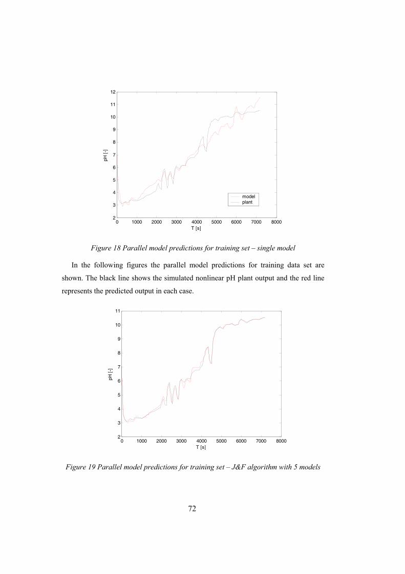
72
0 1000 2000 3000 4000 5000 6000 7000 80002
3
4
5
6
7
8
9
10
11
12
T [s]
pH [
-]
modelplant
Figure 18 Parallel model predictions for training set – single model
In the following figures the parallel model predictions for training data set are
shown. The black line shows the simulated nonlinear pH plant output and the red line
represents the predicted output in each case.
0 1000 2000 3000 4000 5000 6000 7000 80002
3
4
5
6
7
8
9
10
11
T [s]
pH [
-]
Figure 19 Parallel model predictions for training set – J&F algorithm with 5 models

73
0 1000 2000 3000 4000 5000 6000 7000 80002
3
4
5
6
7
8
9
10
11
T [s]
pH [
-]
modelplant
Figure 20 Parallel model predictions for training set – equidistantly distributed models
0 1000 2000 3000 4000 5000 6000 7000 80002
3
4
5
6
7
8
9
10
11
T[s]
pH
Figure 21 Parallel model predictions for training set – SOMA optimized

74
0 1000 2000 3000 4000 5000 6000 7000 80003
4
5
6
7
8
9
10
11
T[s]
pH
Figure 22 Parallel model predictions for test set – SOMA optimized
Network J (Training Data) J (Test Data)
Single ARX model 0.2759 0.3956
5 Equidistantly
distributed Models
0.0117 0.1785
J&F 0.0174 0.2645
SOMA optimization 0.0082 0.1227
Table 2 Comparison of structure identification algorithms
Considerably better performance than the single model is obtained when using
multiple models. Naturally, the J values for the test data are larger than for the training
data in all cases. The values in Table 2 clearly demonstrate the modelling capabilities

75
of the 3 algorithm, with the SOMA evolution algorithm achieving the most accurate
nonlinear representation, but for the highest computational costs. The validity functions
parameters and transfer responses of local model parameters without the offset terms
are shown in Figure 23 and Figure 24. These parameters were obtained with SOMA
optimization of all the parameters. In all these figure one colour corresponds to one
model.
0 100 200 300 400 500 600 700 800 900 10000
0.5
1
1.5
T [s]
Model1Model2Model3Model4Model5
Figure 23 Responses of the local models for a step change of 1ml/s of the flow-rate in
the corresponding operating point

76
3 4 5 6 7 8 9 10 110
0.1
0.2
0.3
0.4
0.5
0.6
0.7
0.8
0.9
1
pH [-]
valid
ity f
unct
ions
Figure 24 Validity functions of the local models
The bias term a0 in the ARX local models provide that the models do not have a
common intersection point in origin as can be seen in Figure 25.
4 6 8 10 12 14 16 18 20 22 242
3
4
5
6
7
8
9
10
11
Q [ml/s]
pH [
-]
Figure 25 Local model network approximation of the nonlinear pH plant
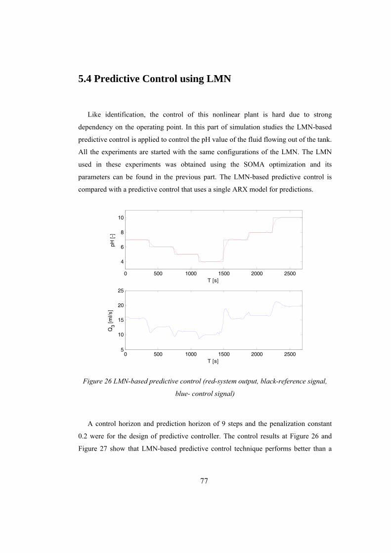
77
5.4 Predictive Control using LMN
Like identification, the control of this nonlinear plant is hard due to strong
dependency on the operating point. In this part of simulation studies the LMN-based
predictive control is applied to control the pH value of the fluid flowing out of the tank.
All the experiments are started with the same configurations of the LMN. The LMN
used in these experiments was obtained using the SOMA optimization and its
parameters can be found in the previous part. The LMN-based predictive control is
compared with a predictive control that uses a single ARX model for predictions.
0 500 1000 1500 2000 2500
4
6
8
10
T [s]
pH [
-]
0 500 1000 1500 2000 25005
10
15
20
25
T [s]
Q3 [
ml/s
]
Figure 26 LMN-based predictive control (red-system output, black-reference signal,
blue- control signal)
A control horizon and prediction horizon of 9 steps and the penalization constant
0.2 were for the design of predictive controller. The control results at Figure 26 and
Figure 27 show that LMN-based predictive control technique performs better than a

78
single model and without steady-state error, which could be expected because a single
ARX model cannot sufficiently represent nonlinear dynamics of the plant.
0 500 1000 1500 2000 2500
4
6
8
10
T [s]
pH [
-]
0 500 1000 1500 2000 25005
10
15
20
25
T [s]
Q3 [
ml/s
]
Figure 27 Predictive control with a single model (red-system output, black-reference
signal, blue- control signal)
5.5 Nonlinear Model Predictive Control
For many-step-ahead control, the influence of the approximation errors may
significantly deteriorate the performance of the predictive control. This can be
remedied by computing the model parameters along the future trajectory. It can be seen
that the controller based on the set of local models performs better than the controller
that is using only a single local model along the whole prediction horizon. The
improvement is larger if the set-point changes cross several local models as can be seen
in Figure 28 between 1200 and 1600s when the plant outputs crosses all five operating
regions with different dynamics. In the experiment the same model as in the previous
examples is used.

79
0 500 1000 1500 2000 2500 3000
4
6
8
10
T [s]
pH [
-]
0 500 1000 1500 2000 2500 30005
10
15
20
25
T [s]
Q3 [
ml/s
]
Figure 28 Comparison of single and multiple model predictions (blue-single
model, red-multiple model )
5.6 Internal Model Control using LMN
The IMC control strategy was applied to control the pH in pH neutralization plant.
The same LMN network scheduled on pH as in the predictive control scheme was used
to model the plant dynamics. The robustness filter
1
0.02
1 0.98FGz
(5.15)
was added to the analytical inverse of the model.

80
0 0.2 0.4 0.6 0.8 1 1.2 1.4 1.6 1.8 2
x 104
3
4
5
6
7
8
9
10
11
T [s]
pH [
-]
0 0.2 0.4 0.6 0.8 1 1.2 1.4 1.6 1.8 2
x 104
5
10
15
20
25
T [s]
Q3 [
ml/s
]
Figure 29 IMC control of pH neutralization plant – set-point tracking
Figure 30 compares the set-point tracking performance of the internal model
controller that uses LMN as internal model with IMC controller that uses only a single
linear model during the whole experiment.

81
0 200 400 600 800 1000 1200 1400 1600 1800 20004
4.5
5
5.5
6
6.5
7
7.5
8
T [s]
pH [
-]
Figure 30 Setpoint tracking (blue –LMN based IMC, red-IMC with linear model)
Figure 31 shows the disturbance rejection capabilities of the IMC controller for the
change of buffer flow rate from 0.55 to 0.15 ml/s at the time t = 200s. This reduction
significantly increases the process gain.
0 200 400 600 800 1000 1200 1400 1600 1800 20007
7.1
7.2
7.3
7.4
7.5
7.6
7.7
7.8
7.9
8
T [s]
pH [
-]
Figure 31 Disturbance rejection (blue –LMN based IMC, red – IMC with linear model)

82
5.7 Laboratory Experiments
This section deals with the application of proposed identification and control
algorithms to real plants. The three-tank model has been chosen for this purpose
because it demonstrates nonlinear behaviour. The laboratory process consists of three
plexiglas cylindrical tanks with identical cross-sections supplied with distilled water.
The liquid levels are measured via the piezoresistive transducers. The laboratory model
is depicted in Figure 32. Water is supplied to the first tank through a controlled pump.
Additionally, another connection to the reservoir lies at each tank, enabling the
introduction of disturbances in the form of leaks. The process is connected to the PC
through a data acquisition board. The identification and control software is written
under MATLAB, using the Real–Time Toolbox to collect data from the process. The
sampling time in all the experiments is set to 1s. The level of the liquid in the first tank
is measured and its value is limited from 0 to 0.6m.
Figure 32 Scheme of the three-tank system
For all the experiments only the tanks h1 and h2 are used. The task is to control the
level in the tank h1 using the voltage applied to the pump 1. The valve between the tank
T1 and T3 is fully open. The valve from the tank T1 is closed and the valve from tank
T3 is partially open.

83
5.8 Nonlinear Modelling and Control of the Two-tank System
A LMN was used to model the nonlinear dynamic relationship between the input
voltage to the pump and the tank level from the process operating data. Since the input
signal in MATLAB units lies in range (-1, 1), signal was shifted by adding 1 to the
input signal. Thus input signal can vary from 0 to 2, where 0 means that the pumps are
off. The process operation is divided into three operating regions. Two data sets were
collected from the process. During the experiments random signal was applied to the
system, with the sampling period of 5 second. The structure of the network was chosen
to be affine local ARX models of the second order.
0 1 2 1 2( 1) ( ) ( 1) ( ) ( 1)y k a a y k a y k b u k b u k (5.16)
The centres of validity function were restricted to lie within the operating region (0
m, 0.1 m), (0.1 m, 0.3 m), (0.3 m, 0.6 m) respectively. The dynamics of the models is
assumed to be stable and the gain of local plant must lie within the limits (0.01 m/MU,
3 m/MU). The previous limits on the process behaviour where translated to the form of
inequalities. For the optimization of the validity function parameters the SOMA
algorithm was used in combination with identification of the local model parameters
using quadratic programming with constraints. Figure 33 shows the training and test
data used for network training and validation. Comparing the step responses of the
local models, one can find that the local model 1 has lower gain and time constant.

84
0 100 200 300 400 500 600 700 800 900 10000
0.2
0.4
T [s]
leve
l [m
]
0 100 200 300 400 500 600 700 800 900 10000
0.5
1
1.5
2
T [s]
u [M
U]
Figure 33 Data for training the LMN
0 100 200 300 400 500 600 700 800 900 10000
0.1
0.2
0.3
0.4
0.5
0.6
0.7
T [s]
leve
l [m
]
plantmodel
Figure 34 LMN prediction on training data

85
The LMN based predictive controller was developed to control the tank level. For
control purposes the constrained optimal control problem is solved with a sampling
period of 5 second and choosing the prediction and control horizons to be Hc =20 and
Hp=20 time steps. The penalization constant = 0.05 was used within the criterion to
stress the importance of the control error. Assuming the physical bounds on the flow-
rate supplied by the pumps, the constraints (0, 2) were imposed into the optimisation
problem. Figure 35 shows the performance of the LMN based predictive controller.
0 500 1000 15000
0.2
0.4
T [s]
leve
l [m
]
0 500 1000 15000
0.5
1
1.5
2
T [s]
u [M
U]
Figure 35 Predictive control with LMN network
To compare the capabilities of the standard linear MPC without any offset
compensation was used in the same experiment. As can be observed the standard MPC
guarantees a stable response without constraints violation, but with static offset. These
deviations can be attributed to the fact that there is no offset compensation. The effect
of the nonlinear model in the predictive controller is minor.

86
0 500 1000 15000
0.2
0.4
T [s]
leve
l [m
]
0 500 1000 15000
0.5
1
1.5
2
T [s]
u [M
U]
Figure 36 Single model predictive control
5.9 Internal Model Control of Two-tank system
The IMC control strategy was applied to the control of the level in the first tank.
The parameters of the model for computation of the model inversion were obtained by
scheduling on the level at the step k-1. Figure 37 demonstrates the performance of the
LMN controller. The filter
11
0.1( )
1 0.9FG zz
(5.17)
was added as part of the controller to improve the robustness to model uncertainty.

87
0 100 200 300 400 500 600 700 800 900 10000
0.2
0.4
T [s]
leve
l [m
]
0 100 200 300 400 500 600 700 800 900 10000
0.5
1
1.5
2
T [s]
u [M
U]
Figure 37 Internal Model Control of the level in the first tank
The IMC control enables easy application of LMN network, where only the
parameters of the filter have to be specified. The control performance of the IMC based
on LMN is also satisfactory.
5.10 Discussion and Concluding Remarks
By using a pH neutralization model plant it has been shown that LMN approach can
provide an improvement in modelling accuracy over a single linear model when used
to represent a dynamics of a chemical plant over a wide operating range. The
modelling performance of J&F algorithm and SOMA optimization algorithm were
evaluated using simulated data from pH neutralization plant. The SOMA optimization
achieves an optimal model but at the expense of intensive computation, while J&F
algorithm produces less accurate model also with local interpretability but with much
less computational effort.

88
The incorporation of the prior knowledge to the parameter identification allows
building models that accurately approximate the plant both globally and locally.
Moreover, it allows modelling of accurate models where less experimental data is
available.
The Model Predictive Control algorithm uses linearization of the LMN model at
current operating point to compensate nonlinearity in process dynamics. The control
algorithm was applied for control of the pH neutralization plant. In experiments better
performance in terms of set-point tracking was achieved comparing to a single model
representation of the process. In order to minimize the steady-state off-sets the internal
loop is implemented to the control loop by changing the reference signals supplied to
standard MPC structure. As could be observed the incorporation of the offset
compensator contributes to remove the static offset caused by the model/plant
mismatch.
A situation when at time k the controller output signal u(k) drives the nonlinear
plant to a operating region represented by another local linear model can occur. In this
case, the control signal is computed for one system and is applied to control another
system. This can badly affect the quality of control if there is a considerable difference
between the dynamics of both models. This can be overcome by using the predicted
trajectory to compute the future linearized models on the predicted trajectory. Higher
value of penalization constant λ in the quadratic cost function J which prevents from
fast changes of the controlled variable can also prevent from mentioned undesired
effects.
LMN with ARX local model can be easily incorporated into the internal model
control framework since the required model inverse can be analytically obtained.
Simulation results for a pH neutralization plant show the significantly improved set-
point tracking and disturbance rejection of both control schemes compared to the single
linear model. The experiments on the three-tank system show that the only small
improvement can be achieved with LMN description of the process. This can be
contributed to the fact that level control in the first tank that is of cylindrical shape is a
weakly nonlinear process.

89
Chapter 6 Concluding Summary
and Future Work
This thesis has examined the LMN structures for identification and control of
nonlinear systems. The idea beyond these networks is to divide the operating range of
nonlinear system into smaller part where the nonlinear system can be represented by a
simple model. In combination with weighting function relatively accurate
approximation can be achieved. LMN models are also easier to interpret than nonlinear
models based on MLP networks and are suitable for building a nonlinear controller that
is composed of local linear controllers. The LMN network can be viewed as
generalization of Radial Basis Function (RBF) network and under specific condition is
functionally equivalent to Takagi-Sugeno fuzzy model. Although normalization of the
weighting function is necessary to provide partition of unity it can also cause several
undesired side-effects such as reactivation or loss of local support.
The learning algorithms can be divided into two classes: local learning techniques,
which are less computationally expensive and create models which are closer to local
linearizations of the nonlinear dynamics and global learning techniques with better
global fit. In Chapter 2 several training algorithms are described and new training
algorithm that utilizes Self-Organizing Migration algorithm for validity function
optimization and quadratic programming for local model parameters estimation is
proposed. This method is able to find improved model compared to the heuristic
Johansen and Foss algorithm. Allowing the splits to be at any point of the operating
space can reduce the number of models and achieve better accuracy. On the other hand,
large number of model evaluations is necessary for optimization. Also the number of
models has to be specified beforehand while heuristic algorithms constantly increase
the number of models and user can choose the best compromise between the accuracy
of the model and its complexity.
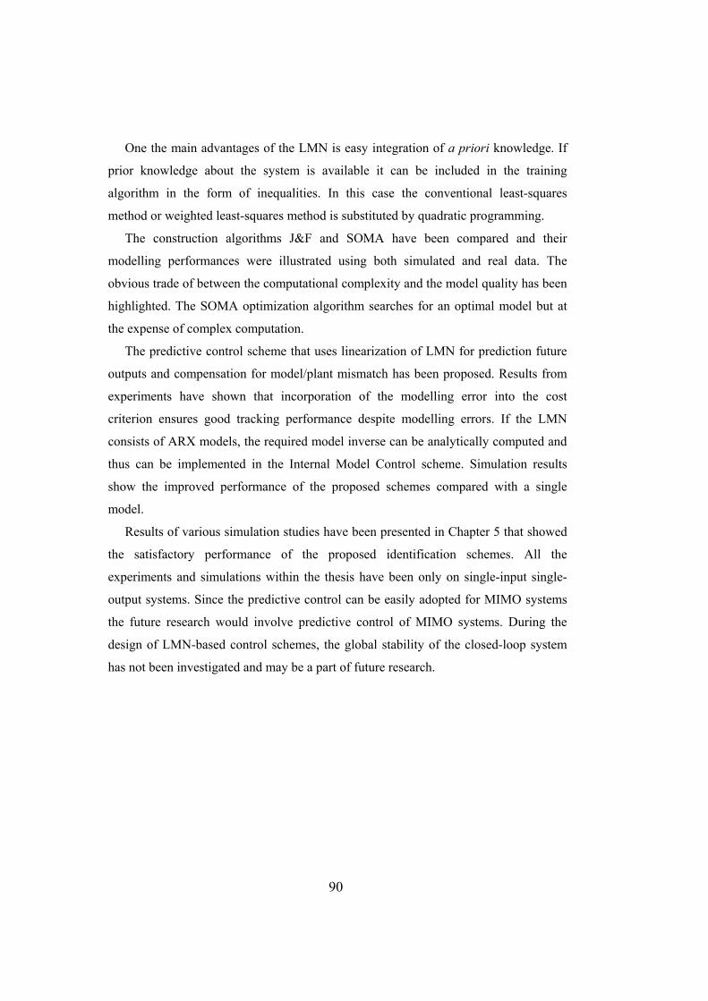
90
One the main advantages of the LMN is easy integration of a priori knowledge. If
prior knowledge about the system is available it can be included in the training
algorithm in the form of inequalities. In this case the conventional least-squares
method or weighted least-squares method is substituted by quadratic programming.
The construction algorithms J&F and SOMA have been compared and their
modelling performances were illustrated using both simulated and real data. The
obvious trade of between the computational complexity and the model quality has been
highlighted. The SOMA optimization algorithm searches for an optimal model but at
the expense of complex computation.
The predictive control scheme that uses linearization of LMN for prediction future
outputs and compensation for model/plant mismatch has been proposed. Results from
experiments have shown that incorporation of the modelling error into the cost
criterion ensures good tracking performance despite modelling errors. If the LMN
consists of ARX models, the required model inverse can be analytically computed and
thus can be implemented in the Internal Model Control scheme. Simulation results
show the improved performance of the proposed schemes compared with a single
model.
Results of various simulation studies have been presented in Chapter 5 that showed
the satisfactory performance of the proposed identification schemes. All the
experiments and simulations within the thesis have been only on single-input single-
output systems. Since the predictive control can be easily adopted for MIMO systems
the future research would involve predictive control of MIMO systems. During the
design of LMN-based control schemes, the global stability of the closed-loop system
has not been investigated and may be a part of future research.

91
Bibliography
[1] CHEN, S., BILLINGS, S.A. Representation of Nonlinear Systems: the
NARMAX model. International Journal of Control. 1989, Vol. 49, no. 3, pages 1013-
1032.
[2] BILLINGS, S., FAKHOURI, S.Y. Identification of systems containing linear
dynamic and static nonlinear elements. Automatica. 1982, Vol. 18, no. 1, pages 15-26.
[3] NARENDRA, K.S., PARTASARANTHY, K. Identification and Control of
Dynamic Systems using neural networks. IEEE Transactions on Neural Networks.
1990, Vol. 1, pages 4-27.
[4] MURRAY-SMITH, R., JOHANSEN, T.A. Multiple Model Approaches to
Modelling and Control. Taylor and Francis, 1997, London, UK.
[5] JOHANSEN, T.A., FOSS, B.A. Identification of nonlinear system structure
and parameters using regime decomposition, Automatica. 1995, Vol. 31.
[6] BILLINGS, S., VOON, W.S.F. Piecewise Linear Identification of Nonlinear
Systems. International Journal of Control. 1987, Vol. 46, pages 215-235.
[7] TAKAGI, K., SUGENO, M.. Derivation of fuzzy control rules from human
operator's control actions. In: Proceedings of IFAC Symposium on Fuzzy Information,
Knowledge Representation and Decision Analysis.1983, pages 55-60.
[8] MCLACHLAN, G., KRISHNAN, T. EM algorithm and Extensions. Wiley,
1997, New York.
[9] XUE, Z.K., LI, S.Y. Multi-model modelling and predictive control based on
local model networks. Control and Intelligent Systems. 2006. Vol. 34, No. 2.
[10] NELLES, O. Orthonormal basis functions for nonlinear system identification
with local linear model trees (LOLIMOT), In: Proceeding of 11th IFAC Symposium on
System Identification.1997, Kitakyushu, Fukuoka, Japan.
[11] MCLOONE, S.F. BROWN, M.D., IRWIN, G.W., LIGHTBODY, G. A hybrid
linear/nonlinear training algorithm for feedforward neural networks. IEEE Trans.
Neural Networks, 1998, vol. 9, no. 4, pages 669-684.
92
[12] SHARMA, S.K., MCLOONE S., IRWIN G.W. Genetic Algorithms For
Simultaneous Identification Of Local Operating Regimes And Local Controller
Network Design. UKACC Control, 2004, Bath, U.K.
[13] MURRAY-SMITH, R., JOHANSEN, T.A. Local Learning in Local Model
Networks. In: Proceedings of 4th IEE International Conference on Artificial Neural
Networks. 1995, Cambridge, UK.
[14] RUSNAK, A., FIKAR, M., NAJIM, K., A. MEZSAROS, A. Generalized
Predictive Control Based on Neural Networks. Neural Processing Letters. 1996, Vol.
4, pages 111-116.
[15] HUNT, K.J., SBARBARO, D. Neural network implementation of non-linear
Internal Model Control and the relationship with Adaptive Inverse Control. In:
Proceedings of IEEE Colloquium on Neural Networks in Control and Modelling of
Industrial Processes. 1991, London, England.
[16] RIVALS, I., PERSONNAZ, L. Internal Model Control Using Neural
Networks. In: Proceedings of the IEEE International Symposium on Industrial
Electronics. 1996, Warsaw, Poland.
[17] SCHOTT, K.D., BEQUETTE, B.W. Control of Nonlinear Chemical Processes
using Multiple-model Adaptive Control. AICHE Annual Meeting. 1994, San
Francisco, California.
[18] DOUGHERTY, D., COOPER, D. A practical multiple model adaptive strategy
for single-loop MPC. Control Engineering Practice. 2003, Vol. 11, pages 141-159.
[19] LI, N., LI, S.Y., XI, Y.G. Multi-model predictive control based on the Takagi-
Sugeno fuzzy models: A case study, Information Science, 2004, Vol. 165, no. 3/4,
pages 247–263.
[20] BROWN, M.D., IRWIN, G.W. Nonlinear Identification and Control of
Turbogenerators Using Local Model Networks. In: Proceeedings of the American
Control Conference. 1999, San Diego, California.
[21] TOWNSEND, S. LIGHTBODY, G., BROWN, M.D., IRWIN, Q.W. Nonlinear
Dynamic Matrix Control Using Local Models. Transactions of the Institute of
Measurement and Control. 1998, Vol. 20, No. 1, pages 47-56.
93
[22] ABONYI, J., NAGY, L., SZEIFERT, F. Fuzzy model-based predictive control
by instantaneous linearization. Fuzzy Sets and Systems. 2001, Vol. 120, no. 2, pages
109-122.
[23] DHARASKAR, K.P, GUPTA, Y.P. Predictive Control of Nonlinear Processes
Using Interpolated Models. Transactions of IChemE. 2000, Vol. 78, pages 573-580.
[24] NARENDRA, K.S., XIANG, C. Adaptive control of discrete-time systems
using multiple models, IEEE Trans. on Automatic Control. 2000, vol. 45, no. 9, pages
1669–1686.
[25] NARENDRA K.S., BALKRISHNAN, J., CILIZ, M.K. Adaptation and
Learning Using Multiple Models, Switching and Tuning. IEEE Control Systems
Magazine. 1995, Vol. 15, no. 3, pages 37-51.
[26] LAN, J., JEONGHO, C., ERDOGMUS, D., PRINCIPE, J., MOTTER, M., XU,
J. Local Linear PID controllers for Nonlinear Control. Control and Intelligent Systems.
2005, Vol. 33.
[27] BANERJEE, A., ARKUN, Y., PEARSON, R., OGUNNAIKE, B. H-infinity
Control of Nonlinear Processes Using Multiple Linear Models. In Multiple Approaches
to Modelling and Control. Taylor and Francis, 1997, London, UK.
[28] MURRAY-SMITH, R. A local model network approach to nonlinear
modelling. Ph. D. thesis.1994, University of Strathclyde, UK.
[29] ALI, A., Application of Local Model Networks to Nonlinear System
Identification and Control. Ph. D. Thesis. 2003, Bochum, Germany.
[30] MCLOONE, S.C., IRWIN, G.W. Continuous-time multiple model networks.
In: Proceedings of the Irish Signals and Systems Conference. 1998, Dublin, Ireland.
[31] BROOMHEAD, D.S., LOWE, D. Multivariable functional interpolation and
adaptive networks. Complex Systems. 1988, Vol. 2, pages 321-355.
[32] POGGIO, T., GIROSI, F. Networks for approximation and learning.
Proceeding of the IEEE, 1990, Vol. 78, no. 9, pages 1481-1497.
[33] SHORTEN, R., MURRAY-SMITH, R. Side effects of Normalising Radial
Basis Function networks. International Journal of Neural Systems. 1996, Vol. 7, No. 2.
[34] JOHANSEN, T.A., SHORTEN, R., MURRAY-SMITH. On the interpretation
and Identification of Dynamic Takagi-Sugeni Fuzzy Models, IEEE Transactions on
Fuzzy Systems. 2000, Vol. 8.

94
[35] GOLUB, G.H., VAN LOAN, C.F. Matrix Computation, Johns Hopkins
University Press, 1996, Baltimore, Maryland.
[36] GOLLEE, H. HUNT, K.J. Nonlinear modelling and control of electrically
stimulated muscle: a local model network approach. International Journal of Control.
1997, Vol. 68, no. 6, pages 1259-1288.
[37] GATH, I., GEVA, A.B. Unsupervised optimal fuzzy clustering. IEEE
Transactions on Pattern Analysis and Machine Intelligence, 1989, Vol. 11, no. 7,
pages 773-781.
[38] ABONYI, J. CHOVAN, T., SZEIFERT, F. Identification of Nonlinear Systems
using Gaussian Mixture of Local Models. Hungarian Journal of Industrial Chemistry.
2001, Vol. 29, pages 134-139.
[39] ABONYI, J. TAR, J., SZEIFERT, F. Identification of MIMO Processes by
Fuzzy Clustering. In: Proceedings of IEEE International Conference on Intelligent
Systems. 2001, Helsinki, Finland.
[40] AARHUS, L. Nonlinear empirical modelling using local PLS models. Ph. D.
Thesis. 1994, University of Oslo, Norway.
[41] KAVLI, T. ASMOD – an adaptive algorithm for adaptive spline modelling of
observation data. International Journal of Control. 1993, Vol. 58, no. 4, pages 947-
967.
[42] JAKUBEK, S., KEUTH, N. A New Training Algorithm for Neuro-Fuzzy
Networks. In: Proceedings of the 2nd International Conference on Informatics in
Control, Automation and Robotics. 2005, Barcelona, Spain.
[43] OMOHUNDRO, S.M. Bumptrees for efficient function, constraints and
classification learning. In: Advances in Neural Information Processing Systems 3.
Morgan Kaufmann Publishers. 1991, San Francisco, CA, pages 693-699.
[44] MCLOONE, S.C. Nonlinear Identification using Local Model Networks. Ph.
D. Thesis. 2000, Queen’s University Belfast, N. Ireland.
[45] MCGINNITY, S., IRWIN, G.W. Comparison of two approaches for multiple-
model identification of a pH neutralisation process. In: Proceedings of European
Control Conference. 1999, Karlsruhe, Germany.
[46] AKAIKE, H. A new look at the statistical model identification. IEEE
Transactions on Automatic Control. 1974, Vol. 19., no. 6, pages 716-726.

95
[47] NELLES, O., FINK, A., ISERMANN, R. Local Linear Model Trees
(LOLIMOT) Toolbox for Nonlinear System Identification. In: Proceedings of the 12th
IFAC Symposium on System Identification. 2000, Santa Barbara, USA.
[48] ZELINKA, I. SOMA – Self Organizing Migrating Algorithm, Chapter 7 in
Babu, B.V., Onwubolu, G.(eds), New Optimization Techniques in Engineering,
Springer-Verlag, 2004.
[49] LJUNG, L. System Identification: Theory for Users. Prentice Hall. 1999,
Upper Saddle River, New Jersey.
[50] A ABONYI, J., BABUSKA, R., VERBRUGGEN H., SZEIFERT, F.
Incorporating prior knowledge in fuzzy model identification. International Journal of
Systems Science. 2000, Vol. 31.
[51] CAMACHO, E.F., BORDONS, C. Model Predictive Control. Second Edition.
Springer, 2004.
[52] HABER, R., BARS, R., LENGYEL, O. Long-range Predictive Control of the
Parametric Hammerstein Model, In: Proceedings of the IFAC Symposium on
Nonlinear Control Systems Design. 1998, Enschede, The Netherlands.
[53] HABER, R., BARS, R., LENGYEL, O. Three extended horizon adaptive
nonlinear predictive control schemes based on the parametric Volterra model. In:
Proceedings of the European Control Conference. 1999, Karlsruhe, Germany.
[54] SBARBARO, D. Local Laguerre models. In: Multiple Model Approaches to
Modelling and Conrol. Ed. R. Murray-Smith and T.A. Johansen. Taylor and Francis.
1997, London, UK.
[55] ARAHAL, M.R., BEREGUEL, M., CAMACHO, E.F. Neural identification
applied to predictive control of a solar plant. Control Engineering Practice. 1998,
Vol.6, pages 333-334.
[56] KARLA, V.R., BAKKER, H.H.C. Neural-network-based Model Predictive
Control: A Case Study. 2nd New Zealand Two-Stream International Conference on
Artificial Neural Networks and Expert Systems (ANNES '95). 1995, Dunedin, New
Zealand.
[57] ZHANG, J. , MORRIS, A.J. Long Range Predictive Control of Nonlinear
Processes Based on Recurrent Neuro-Fuzzy Network Models. Neural Computing and
Applications. 2000, Vol. 9, No 1.

96
[58] GILL, P., HENRIQUES, J., DOURADO, A., DUARTE-RAMOS, H. Extended
Neural Model Predictive Control of Non-linear Systems. In: Proceedings of the
IASTED Conference on Artificial Intelligence and Soft Computing. 2000, Banff,
Alberta, Canada.
[59] HUANGH, Y.L., LOU, H.H., GONG, J.P., EDGAR, T.F. Fuzzy Model
Predictive Control. IEEE Transactions on Fuzzy Systems. 2000,Vol. 8, No. 6.
[60] MOLLOV, S., VEEN, P., BABUSKA, R. ABONYU, J., ROUBOS, J.,
VERBRUGGEN, H.B. Extraction of local linear models from Takagi-Sugeno fuzzy
model with application to model-based predictive control. In: Proceedings of 7th
European Congress on Intelligent Techniques and Soft Computing. 1999, Aachen,
Germany.
[61] MORARI, M., ZAFIROU, E. Robust Process Control, Prentice Hall, 1989,
New Jersey.
[62] NAHAS, E. P., HENSON, M.A., SEBORG, D.E. Nonlinear internal model
control strategy for neural network models. Computers Chemical Engineering. 1992,
Vol. 16, No. 2, pages 1039-1057.
[63] HU, Q., SAHA, P., RANGAIAH, G.P. Experimental evaluation of an
augmented IMC for nonlinear systems. Control Engineering Practice. 2000. Vol. 8,
pages 1167-1176.
[64] HALL, R.C., SEBORG, D.E. Modelling and self-tuning control of a
multivariable pH neutralization process. Part I: Modelling and multiloop control. In:
Proceeding of American Control Conference. 1989, Pittsburgh.
[65] FINK, A., NELLES, O. Nonlinear Internal Model Control Based on Local
Linear Neural Networks. In: Proceeding of the IEEE Conference Systems, Man and
Cybernetics. 2001, Tucson, Arizona.

97
Publications
Most of the work in this thesis has been presented in international and national
conferences. The conferences are listed below:
1. Novák, J., V. Bobál, J. Vojtěšek (2006). Nonlinear Internal Model Control of
CSTR, In: Proceedings of the Portuguese Conference on Automatic Control
2006. Lisboa, Portugal.
2. Novák, J., V. Bobál (2006). CSTR Control using Multiple Models. In:
Proceeding of International Conference Technical Computing Prague
(TCP’06). Prague, Czech Republic.
3. Novák, J., M. Červenka, V. Bobál (2006). Optimization of Local Model
Network parameters. In: Proceedings of 7th International Scientific-Technical
Conference Process Control. Kouty nad Desnou, Czech Republic.
4. Novák, J., V. Bobál, (2005). Control of DR300 Servo using Local Model
Network. 9th International Conference „Trends in the Development of
Machinery and Associated Technology“, Antalya, Turkey.
5. Novák, J., V. Bobál (2005). Adaptive Control using Multiple Models. In:
Proceedings of 15th International Conference on Process Control, Štrbské
pleso, Slovakia.
6. Novák, J., V. Bobál (2005). Control of DR300 Servo using Multiple Models.
In: Proceeding of International Conference Technical Computing Prague
(TCP’05). Prague, Czech Republic.
7. Novák, J., V. Bobál (2005). Řízení servomechanismu Amira DR300. In:
Proceedings of the Automatizace, Regulace a Procesy Conference (In Czech).
Brno, Czech Republic.
8. Novák, J., V. Bobál (2004). Intelligent Adaptive Control using Multiple
Models. In: Proceedings of the 22nd IASTED International Conference on
Modelling, Identification and Control. Grindelwald, Switzerland.

98
Other publication activity:
9. Novák, J., P. Chalupa and V. Bobál (2006). New Laboratory Course
For Control Education. In: Proceedings of the IFAC conference on
Advances in Control Education 2006. Madrid, Spain.

99
Curriculum Vitae Personal data:
Name: Jakub Novák
Date of Birth: 8.12.1978
Place of Birth: Zlín
Address: Lazy 1/1762 Zlín 76001
E-mail: [email protected]
Education:
2005 –till now: Tomas Bata University, Center of Applied Cybernetics
Research interests: Prediction of electricity consumption
Stability of Electricity Supply Network
2002 –till now: Tomas Bata University, PhD. study
Research interests: Adaptive control using multiple models
Local model networks
1997 – 2002: Tomas Bata University, Mr.Sc. study in the department of Automation
and Control


![Nonlinear System Identification[Oliver Nelles]](https://img.dokumen.tips/doc/110x75/563dba91550346aa9aa6c147/nonlinear-system-identificationoliver-nelles.jpg)


