Nonlinear Functions

By definition, nonlinear functions are functions which are not linear. Quadratic functions are one type of nonlinear function. We discuss several other nonlinear functions in this section. A. Absolute Value Recall that the absolute value of a real number x is defined as

if 0if x<0

x xx

x≥⎧

= ⎨−⎩

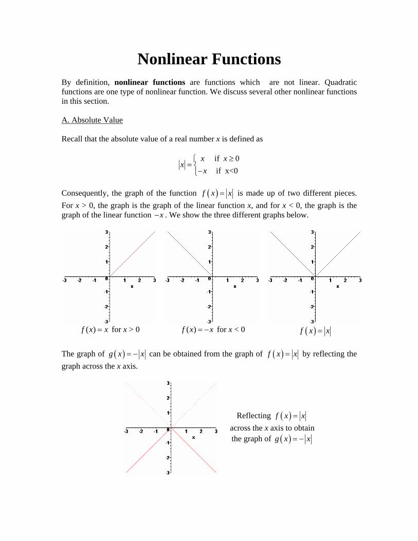
Consequently, the graph of the function ( )f x x= is made up of two different pieces. For x > 0, the graph is the graph of the linear function x, and for x < 0, the graph is the graph of the linear function x− . We show the three different graphs below.

( )f x x= for x > 0 ( )f x x= − for x < 0 ( )f x x=

The graph of ( )g x x= − can be obtained from the graph of ( )f x x= by reflecting the graph across the x axis.

Reflecting ( )f x x= across the x axis to obtain the graph of ( )g x x= −

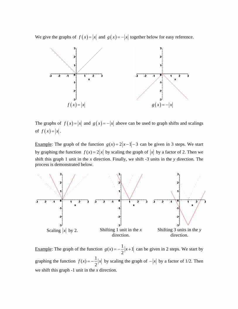
We give the graphs of ( )f x x= and ( )g x x= − together below for easy reference.

( )f x x= ( )g x x= −

The graphs of ( )f x x= and ( )g x x= − above can be used to graph shifts and scalings

of ( )f x x= . Example: The graph of the function ( ) 2 1 3g x x= − − can be given in 3 steps. We start

by graphing the function ( ) 2f x x= by scaling the graph of x by a factor of 2. Then we shift this graph 1 unit in the x direction. Finally, we shift -3 units in the y direction. The process is demonstrated below.

Scaling x by 2. Shifting 1 unit in the x

direction. Shifting 3 units in the y

direction.

Example: The graph of the function 1( ) 12

g x x= − + can be given in 2 steps. We start by

graphing the function 1( )2

f x x= − by scaling the graph of x− by a factor of 1/2. Then

we shift this graph -1 unit in the x direction.

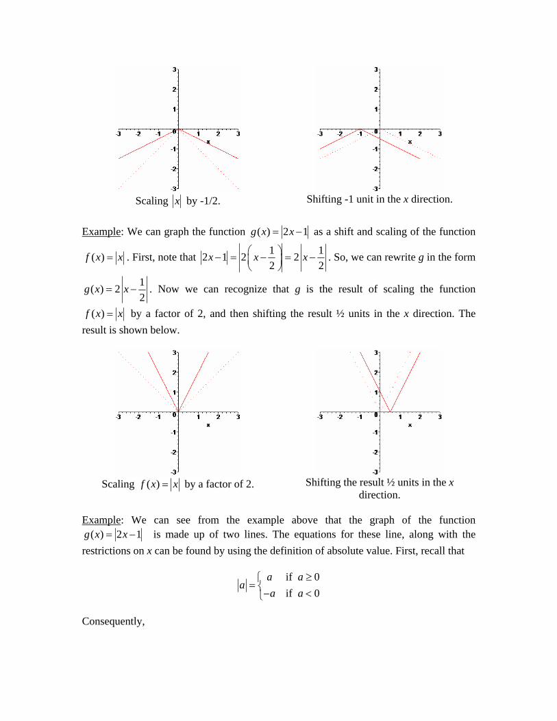
Scaling x by -1/2. Shifting -1 unit in the x direction.

Example: We can graph the function ( ) 2 1g x x= − as a shift and scaling of the function

( )f x x= . First, note that 1 12 1 2 22 2

x x x⎛ ⎞− = − = −⎜ ⎟⎝ ⎠

. So, we can rewrite g in the form

1( ) 22

g x x= − . Now we can recognize that g is the result of scaling the function

( )f x x= by a factor of 2, and then shifting the result ½ units in the x direction. The result is shown below.

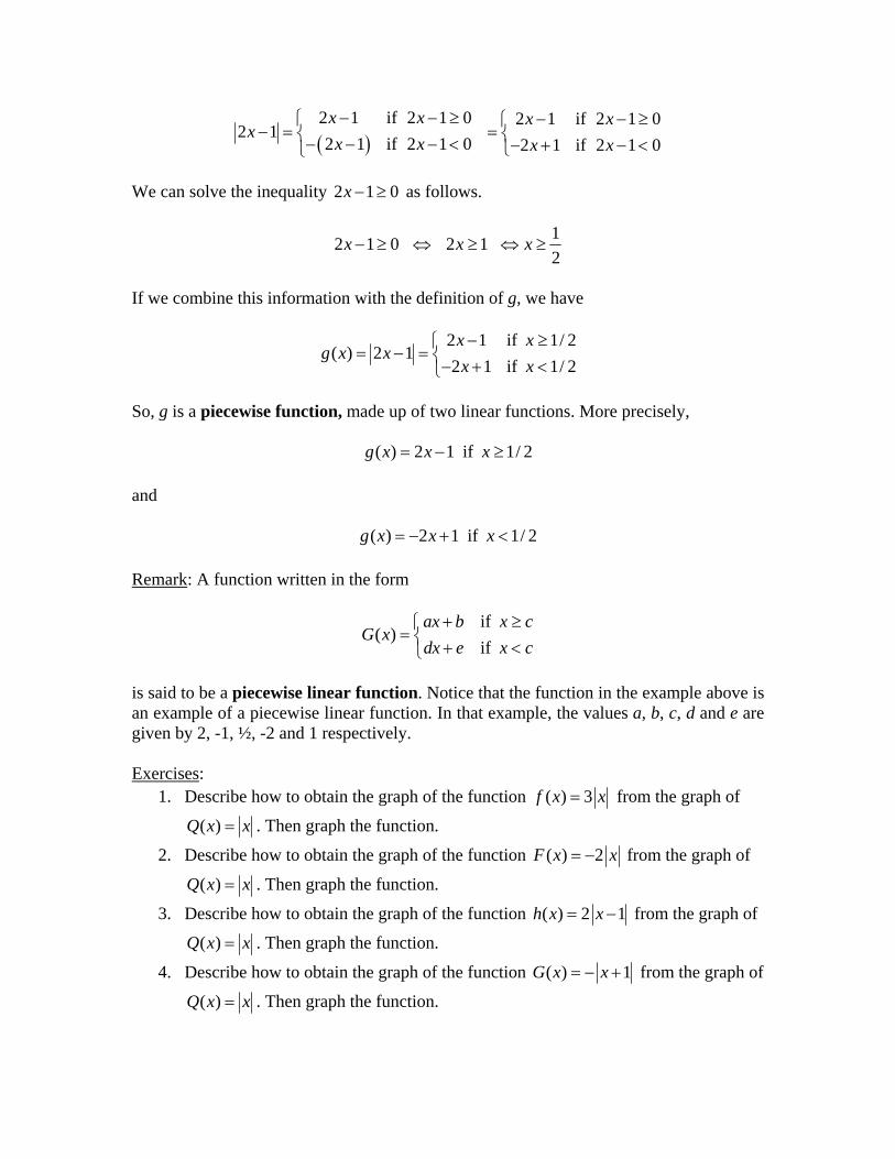
Scaling ( )f x x= by a factor of 2. Shifting the result ½ units in the x

direction. Example: We can see from the example above that the graph of the function

( ) 2 1g x x= − is made up of two lines. The equations for these line, along with the restrictions on x can be found by using the definition of absolute value. First, recall that

if 0if 0

a aa

a a≥⎧

= ⎨− <⎩

Consequently,

( )2 1 if 2 1 0 2 1 if 2 1 0

2 1 2 1 if 2 1 0 2 1 if 2 1 0x x x x

xx x x x− − ≥ − − ≥⎧ ⎧

− = =⎨ ⎨− − − < − + − <⎩⎩

We can solve the inequality 2 1 0x − ≥ as follows.

12 1 0 2 1 2

x x x− ≥ ⇔ ≥ ⇔ ≥

If we combine this information with the definition of g, we have

2 1 if 1/ 2( ) 2 1

2 1 if 1/ 2x x

g x xx x− ≥⎧

= − = ⎨− + <⎩

So, g is a piecewise function, made up of two linear functions. More precisely,

( ) 2 1 if 1/ 2g x x x= − ≥

and

( ) 2 1 if 1/ 2g x x x= − + <

Remark: A function written in the form

if ( )

if ax b x c

G xdx e x c

+ ≥⎧= ⎨ + <⎩

is said to be a piecewise linear function. Notice that the function in the example above is an example of a piecewise linear function. In that example, the values a, b, c, d and e are given by 2, -1, ½, -2 and 1 respectively. Exercises:

1. Describe how to obtain the graph of the function ( ) 3f x x= from the graph of

( )Q x x= . Then graph the function.

2. Describe how to obtain the graph of the function ( ) 2F x x= − from the graph of

( )Q x x= . Then graph the function.

3. Describe how to obtain the graph of the function ( ) 2 1h x x= − from the graph of

( )Q x x= . Then graph the function.

4. Describe how to obtain the graph of the function ( ) 1G x x= − + from the graph of

( )Q x x= . Then graph the function.

5. Describe how to obtain the graph of the function 1( ) 1 22

R x x= − + from the

graph of ( )Q x x= . Then graph the function.

6. Describe how to obtain the graph of the function ( ) 1 3T x x= + − from the graph

of ( )Q x x= . Then graph the function.

7. Describe how to obtain the graph of the function ( ) 3 2H x x= − from the graph

of ( )Q x x= . Then graph the function.

8. Describe how to obtain the graph of the function ( ) 2 4 1H x x= + − from the

graph of ( )Q x x= . Then graph the function.

9. Use the definition of absolute value to write the function ( ) 1G x x= − + as a piecewise linear function.

10. Use the definition of absolute value to write the function ( ) 1 3T x x= + − as a piecewise linear function.

11. Use the definition of absolute value to write the function 1( ) 1 22

R x x= − + as a

piecewise linear function. 12. Use the definition of absolute value to write the function ( ) 3 2H x x= − as a

piecewise linear function. 13. Use the definition of absolute value to write the function ( ) 2 4 1M x x= + − as a

piecewise linear function. B. Polynomial Functions We have already seen some special types of polynomial functions. A linear function

( )f x mx b= + is a first degree polynomial function. A quadratic function

2( )g x ax bx c= + +

is a second degree polynomial function. In general, an thn degree polynomial function is a function of the form

1 0( ) nnF x a x a x a= + + +

where { }0,1, 2,...n∈ and 1 0,..., ,na a a ∈ with 0na ≠ . Examples:

1. ( ) 1f x = is a polynomial of degree 0.

2. 1 4( )2 3

H x x= − is a polynomial of degree 1.

3. 2 3( ) 311

R x x x= − + is a polynomial of degree 2.

4. 7 24( ) 3 33

F x x x x= − − + is a polynomial of degree 7.

The graphs of polynomial functions can sometimes be very complicated. For example the

graph of 7 4 21( ) 2 4 1100

F x x x x x= − − − − + is shown below.

7 4 21( ) 2 4 1

100F x x x x x= − − − − +

One class of polynomial functions which have predictable graphs is given by

( ) nF x x=

where { }0,1, 2,...n∈ . If n is an even natural number, then the graph of ( ) nF x x= has a

graph that is similar to the graph of 2( )f x x= .

( ) nF x x= when n is even.

Although these graphs are similar, they are not called parabolas. The graph of 3( )f x x= is shown below along with a table of values for the function.

x 3x -2 -8

-1.8 -5.832 -1.6 -4.096 -1.4 -2.744 -1.2 -1.728 -1 -1

-0.8 -0.512 -0.6 -0.216 -0.4 -0.064 -0.2 -0.008

0 0 0.2 0.008 0.4 0.064 0.6 0.216 0.8 0.512 1 1

1.2 1.728 1.4 2.744 1.6 4.096 1.8 5.832 2 8

-10

-8

-6

-4

-2

0

2

4

6

8

10

-3 -2 -1 0 1 2 3

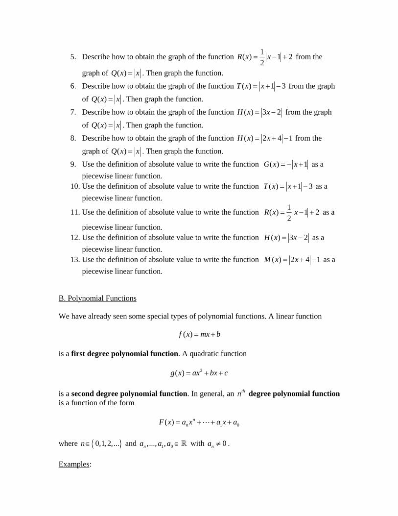
If 3n ≥ is an odd natural number, then the graph of ( ) nF x x= has a graph that is similar to the graph of 3( )f x x= .

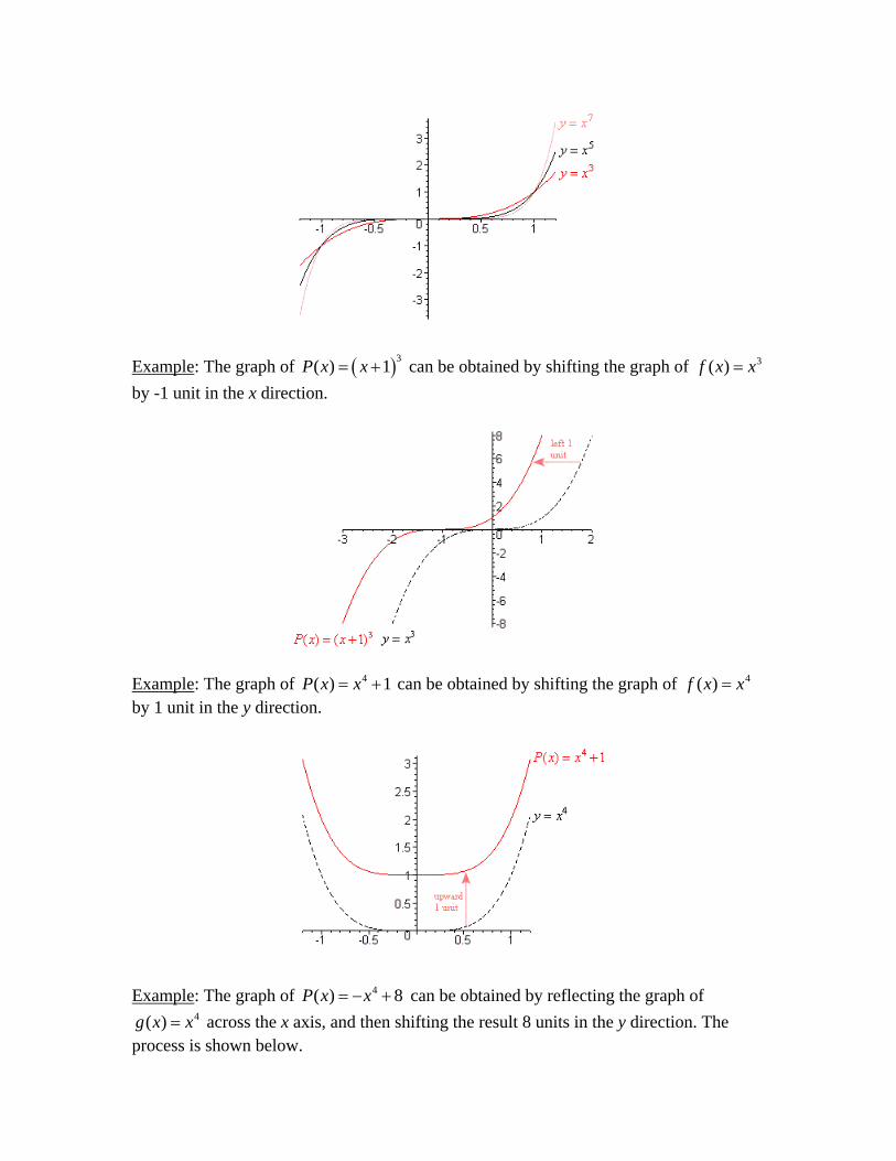
Example: The graph of ( )3( ) 1P x x= + can be obtained by shifting the graph of 3( )f x x= by -1 unit in the x direction.

Example: The graph of 4( ) 1P x x= + can be obtained by shifting the graph of 4( )f x x= by 1 unit in the y direction.

Example: The graph of 4( ) 8P x x= − + can be obtained by reflecting the graph of

4( )g x x= across the x axis, and then shifting the result 8 units in the y direction. The process is shown below.

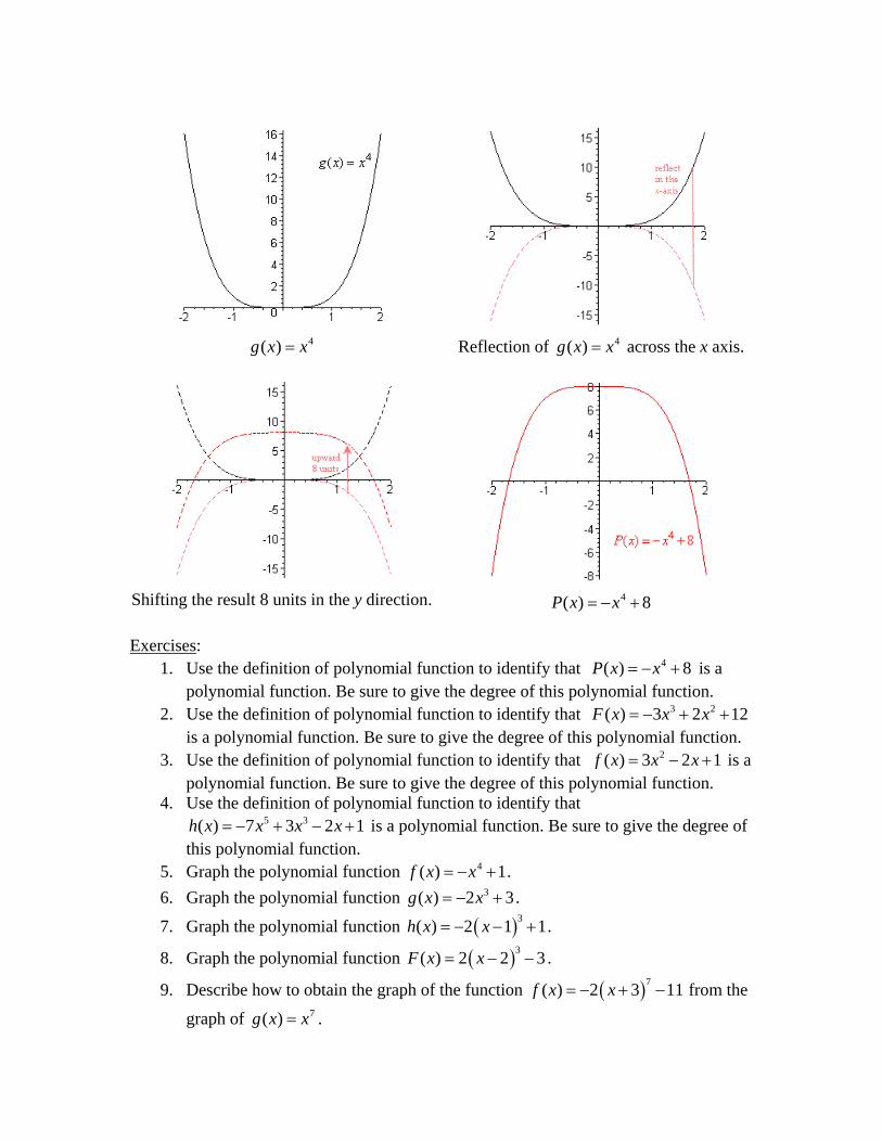
4( )g x x= Reflection of 4( )g x x= across the x axis.

Shifting the result 8 units in the y direction. 4( ) 8P x x= − + Exercises:

1. Use the definition of polynomial function to identify that 4( ) 8P x x= − + is a polynomial function. Be sure to give the degree of this polynomial function.

2. Use the definition of polynomial function to identify that 3 2( ) 3 2 12F x x x= − + + is a polynomial function. Be sure to give the degree of this polynomial function.

3. Use the definition of polynomial function to identify that 2( ) 3 2 1f x x x= − + is a polynomial function. Be sure to give the degree of this polynomial function.

4. Use the definition of polynomial function to identify that 5 3( ) 7 3 2 1h x x x x= − + − + is a polynomial function. Be sure to give the degree of

this polynomial function. 5. Graph the polynomial function 4( ) 1f x x= − + . 6. Graph the polynomial function 3( ) 2 3g x x= − + .

7. Graph the polynomial function ( )3( ) 2 1 1h x x= − − + .

8. Graph the polynomial function ( )3( ) 2 2 3F x x= − − .

9. Describe how to obtain the graph of the function ( )7( ) 2 3 11f x x= − + − from the

graph of 7( )g x x= .

10. Describe how to obtain the graph of the function ( )12( ) 3 2 5f x x= − + from the

graph of 12( )g x x= .

11. Describe how to obtain the graph of the function ( )7( ) 4 1 2f x x= + + from the

graph of 7( )g x x= . Hint: 14 1 44

x x⎛ ⎞+ = +⎜ ⎟⎝ ⎠

.

C. Rational Functions Rational functions are functions which can be written in the form

( )( )( )

P xf xQ x

=

where ( )P x and ( )Q x are polynomial functions. Examples:

1. 2( ) 3 2 1f x x x= − + is a rational function since it can be written as a quotient of the 2nd degree polynomial function 2( ) 3 2 1P x x x= − + and the 0th degree polynomial function ( ) 1Q x = . In general, all polynomial functions are rational functions.

2. 2 2( )

3 5xf xx−

=+

is a rational function since it is the quotient of polynomials with 2( ) 2P x x= − and ( ) 3 5Q x x= + .

Remark: The domain of a rational function is the set of all values of x where the denominator Q(x) is nonzero. The graphs of rational functions can be very complicated. For example, the graph of

3 2

3 2

4 2 1( )2 2 4x x xf x

x x x− − − −

=− −

is given below.

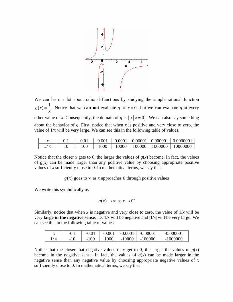
We can learn a lot about rational functions by studying the simple rational function

1( )g xx

= . Notice that we can not evaluate g at 0x = , but we can evaluate g at every

other value of x. Consequently, the domain of g is { }0x x ≠ . We can also say something about the behavior of g. First, notice that when x is positive and very close to zero, the value of 1/x will be very large. We can see this in the following table of values.

x 0.1 0.01 0.001 0.0001 0.00001 0.000001 0.0000001 1/ x 10 100 1000 10000 100000 1000000 10000000

Notice that the closer x gets to 0, the larger the values of g(x) become. In fact, the values of g(x) can be made larger than any positive value by choosing appropriate positive values of x sufficiently close to 0. In mathematical terms, we say that

( ) goes to as approaches 0 through positive valuesg x x∞

We write this symbolically as

( ) as 0g x x +→∞ →

Similarly, notice that when x is negative and very close to zero, the value of 1/x will be very large in the negative sense; i.e. 1/x will be negative and |1/x| will be very large. We can see this in the following table of values.

x -0.1 -0.01 -0.001 -0.0001 -0.00001 -0.000001 1/ x -10 -100 1000 -10000 -100000 -1000000

Notice that the closer that negative values of x get to 0, the larger the values of g(x) become in the negative sense. In fact, the values of g(x) can be made larger in the negative sense than any negative value by choosing appropriate negative values of x sufficiently close to 0. In mathematical terms, we say that

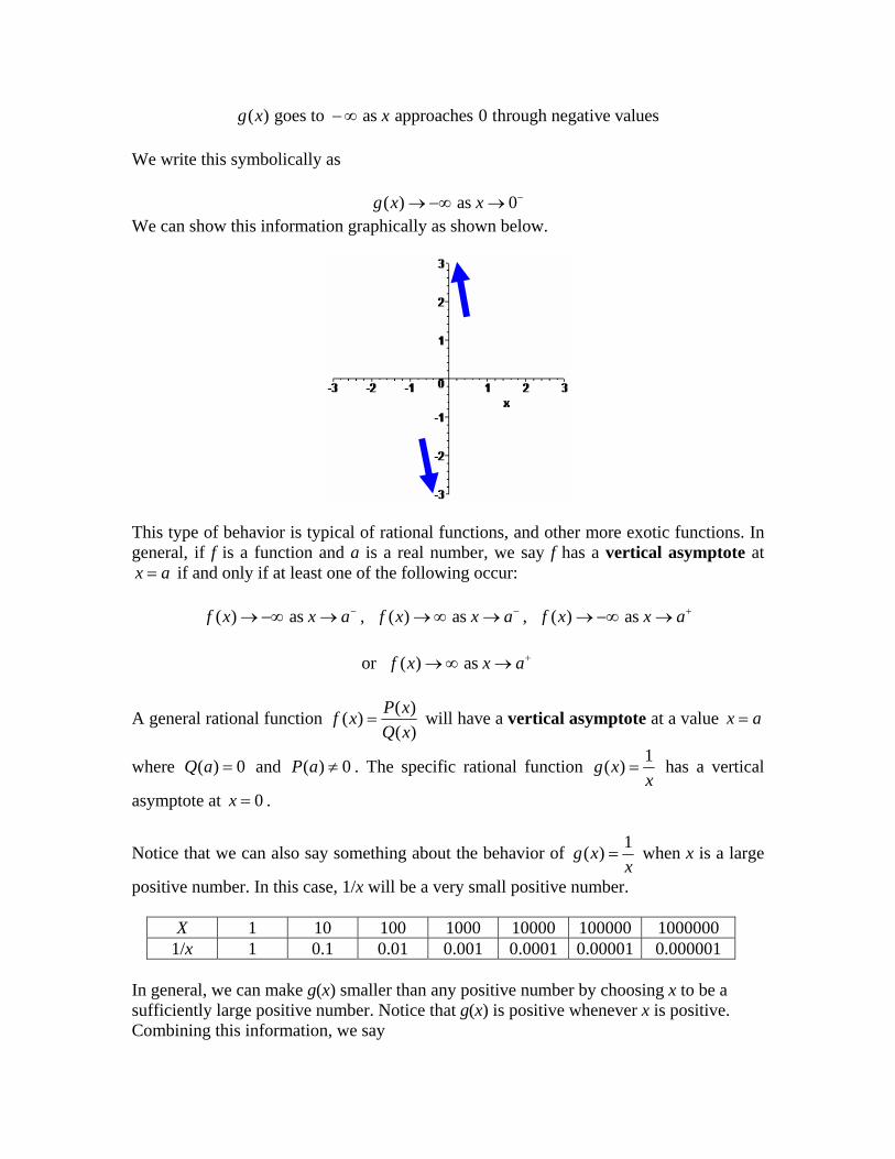
( ) goes to as approaches 0 through negative valuesg x x−∞

We write this symbolically as

( ) as 0g x x −→ −∞ → We can show this information graphically as shown below.

This type of behavior is typical of rational functions, and other more exotic functions. In general, if f is a function and a is a real number, we say f has a vertical asymptote at x a= if and only if at least one of the following occur:

( ) as f x x a−→ −∞ → , ( ) as f x x a−→∞ → , ( ) as f x x a+→ −∞ →

or ( ) as f x x a+→∞ →

A general rational function ( )( )( )

P xf xQ x

= will have a vertical asymptote at a value x a=

where ( ) 0Q a = and ( ) 0P a ≠ . The specific rational function 1( )g xx

= has a vertical

asymptote at 0x = .

Notice that we can also say something about the behavior of 1( )g xx

= when x is a large

positive number. In this case, 1/x will be a very small positive number.

X 1 10 100 1000 10000 100000 1000000 1/x 1 0.1 0.01 0.001 0.0001 0.00001 0.000001

In general, we can make g(x) smaller than any positive number by choosing x to be a sufficiently large positive number. Notice that g(x) is positive whenever x is positive. Combining this information, we say

( ) goes to 0 through positive values as approaches g x x ∞

We write this symbolically as

( ) 0 as g x x+→ →∞ Similarly, we can say something about the behavior of g(x) when x is a large negative number (i.e. large in the negative sense). In this case, 1/x will be a negative number which is very close to 0.

x -1 -10 -100 -1000 -10000 -100000 1/x -1 -0.1 -0.01 -0.001 -0.0001 -0.00001

In general, we can make g(x) closer to 0 than any negative number by choosing x sufficiently large in the negative sense. Notice that g(x) is negative whenever x is negative. Combining this information, we say

( ) goes to 0 through negative values as approaches g x x −∞

We write this symbolically as

( ) 0 as g x x−→ → −∞

We incorporate this information into our earlier picture below.

This type of behavior is typical of more general rational functions ( )( )( )

P xf xQ x

=

whenever the degree of ( )P x is less than or equal to the degree of ( )Q x . In general, if c is a real number, we say f has a horizontal asymptote at y c= if and only if at least one of the following occur:

( ) as f x c x→ →−∞ or ( ) as f x c x→ →∞

The function 1( )g xx

= has a horizontal asymptote at 0y = .

A general rational function ( )( )( )

P xf xQ x

= will have the horizontal asymptote 0y = if

and only if the degree of ( )P x is less than the degree of ( )Q x . In the case when the degree of ( )P x is equal to the degree of ( )Q x , if

1 0( ) nnP x a x a x a= + + +

and

1 0( ) nnQ x b x b x b= + + +

are polynomial functions of degree n, then ( )( )( )

P xf xQ x

= will have the horizontal

asymptote n

n

ayb

= .

We plot a set of data points below to obtain a graph of 1( )g xx

= . Notice how the

behavior of the graph incorporates our comments from above.

x 1/x -3.00 -0.33 -2.50 -0.40 -2.00 -0.50 -1.50 -0.67 -1.00 -1.00 -0.50 -2.00 -0.33 -3.00 0.33 3.00 0.50 2.00 1.00 1.00 1.50 0.67 2.00 0.50 2.50 0.40 3.00 0.33

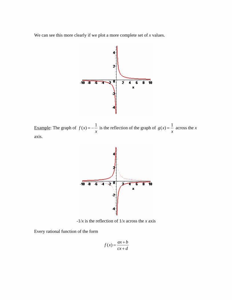
We can see this more clearly if we plot a more complete set of x values.

Example: The graph of 1( )f xx

= − is the reflection of the graph of 1( )g xx

= across the x

axis.

-1/x is the reflection of 1/x across the x axis

Every rational function of the form

( ) ax bf xcx d

+=

+

(with 0c ≠ ) is a scaling, reflection, and/or shift of 1( )g xx

= . We can see this by making

the following series of algebraic manipulations:

2

( )

1

1/

ax bf xcx d

a cx bc cx d cx da cx d a d bc cx d c cx d cx d

a bc adc c cx da bc adc c x d c

+=

+⎛ ⎞= +⎜ ⎟ + +⎝ ⎠

+⎛ ⎞ ⎛ ⎞= − +⎜ ⎟ ⎜ ⎟+ + +⎝ ⎠ ⎝ ⎠−⎛ ⎞= + ⎜ ⎟ +⎝ ⎠−⎛ ⎞= + ⎜ ⎟ +⎝ ⎠

The calculations above show that the graph of f can be obtained by shifting the graph of

1( )g xx

= by –d/c units in the x direction, then scaling the result by 2

bc adc− , and finally

shifting by a/c units in the y direction. Notice that if 2 0bc adc−

< then the scaling also

incorporates a reflection across the x axis. This function will have a vertical asymptote at x = –d/c and a horizontal asymptote at y = a/c.

Example: Consider the rational function 3( )2 4xf xx+

=−

. Notice that the denominator is

zero when 2 4 0x − = , and this occurs when x = 2. Also, notice that the numerator is not zero at this value of x. As a result, f has a vertical asymptote at x = 2. Also, in this case, the polynomials in the numerator and denominator have the same degree (namely 1). So, from the leading coefficients, we know that f has a horizontal asymptote at y = ½. Finally, we can see that

( )( )

3( )2 41 2 32 2 4 2 41 2 4 1 4 32 2 4 2 2 4 2 4

4 2 31 12 2 2 4

1 5 12 2 2

xf xx

xx xxx x x

x

x

+=

−⎛ ⎞= +⎜ ⎟ − −⎝ ⎠

−⎛ ⎞ ⎛ ⎞= + +⎜ ⎟ ⎜ ⎟− − −⎝ ⎠ ⎝ ⎠⎛ ⎞+

= + ⎜ ⎟ +⎝ ⎠⎛ ⎞= + ⎜ ⎟ +⎝ ⎠

Therefore, the graph of f can be obtained from the graph of 1( )g xx

= by scaling by a

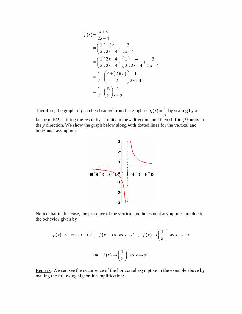
factor of 5/2, shifting the result by -2 units in the x direction, and then shifting ½ units in the y direction. We show the graph below along with dotted lines for the vertical and horizontal asymptotes.

Notice that in this case, the presence of the vertical and horizontal asymptotes are due to the behavior given by

( ) as 2f x x −→ −∞ → , ( ) as 2f x x +→∞ → , 1( ) as 2

f x x−

⎛ ⎞→ → −∞⎜ ⎟⎝ ⎠

and 1( ) as 2

f x x+

⎛ ⎞→ →∞⎜ ⎟⎝ ⎠

.

Remark: We can see the occurrence of the horizontal asymptote in the example above by making the following algebraic simplification:

3 1 3/( )2 4 2 4 /x xf xx x+ +

= =− −

whenever 0x ≠ . Now, notice that for large values of x (in either the negative or positive sense) the values 3/x and -4/x will be very close to zero. Consequently,

3 1 3/ 1( ) as 2 4 2 4 / 2x xf x xx x+ +

= = → →±∞− −

This process can always be used to observe a horizontal asymptote of a rational function.

Example: Consider the rational function 3 1( )3

xr xx+

=−

. Notice that the denominator is

zero at x = 3, and the numerator is not zero at x = 3. Consequently, r has a vertical asymptote at x = 3. Also, the degree of the numerator is the same as the degree of the denominator (namely 1), so the leading coefficients tell us there is a horizontal asymptote at y = 3/1 = 3. Notice that we can also see this by performing a calculation similar to the one shown in the remark above, since

3 1 3 1/( )3 1 3/

x xr xx x+ +

= =− −

whenever 0x ≠ . Consequently,

3 1 3 1/ 3( ) 3 as 3 1 3/ 1

x xr x xx x+ +

= = → = → ±∞− −

Before we give the graph, we note that the y intercept occurs where x = 0, and

( )( )3 0 1

(0) 1/ 30 3

r+

= = −−

. The x intercept occurs where r(x) = 0, and

3 1 0 1/ 3x x+ = ⇔ = −

Finally,

3 1( )3

133 33 3 13 33 3 3

13 43

xr xx

xx xxx x x

x

+=

−

= +− −−

= + +− − −

= +−

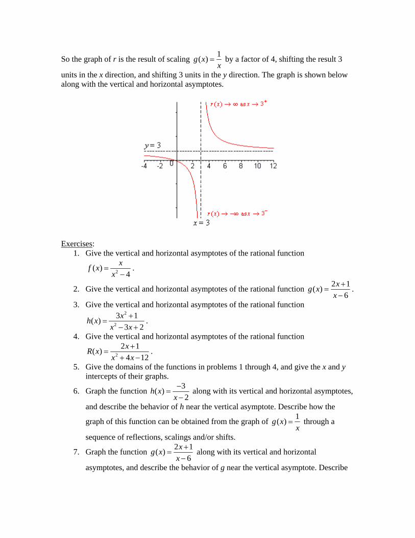
So the graph of r is the result of scaling 1( )g xx

= by a factor of 4, shifting the result 3

units in the x direction, and shifting 3 units in the y direction. The graph is shown below along with the vertical and horizontal asymptotes.

Exercises:

1. Give the vertical and horizontal asymptotes of the rational function

2( )4

xf xx

=−

.

2. Give the vertical and horizontal asymptotes of the rational function 2 1( )6

xg xx+

=−

.

3. Give the vertical and horizontal asymptotes of the rational function 2

2

3 1( )3 2

xh xx x

+=

− +.

4. Give the vertical and horizontal asymptotes of the rational function

2

2 1( )4 12xR x

x x+

=+ −

.

5. Give the domains of the functions in problems 1 through 4, and give the x and y intercepts of their graphs.

6. Graph the function 3( )2

h xx−

=−

along with its vertical and horizontal asymptotes,

and describe the behavior of h near the vertical asymptote. Describe how the

graph of this function can be obtained from the graph of 1( )g xx

= through a

sequence of reflections, scalings and/or shifts.

7. Graph the function 2 1( )6

xg xx+

=−

along with its vertical and horizontal

asymptotes, and describe the behavior of g near the vertical asymptote. Describe

how the graph of this function can be obtained from the graph of 1( )R xx

=

through a sequence of reflections, scalings and/or shifts.

8. Graph the function 3 6( )1

xf xx

− +=

+ along with its vertical and horizontal

asymptotes, and describe the behavior of f near the vertical asymptote. Describe

how the graph of this function can be obtained from the graph of 1( )g xx

=

through a sequence of reflections, scalings and/or shifts. D. Exponential Functions Functions of the form

( ) xf x a= with 0a >

are called exponential functions. Notice that this function is very boring if a = 1. The behavior is very different depending upon whether 0 < a < 1 or a > 1. We illustrate this by considering the cases a = ½ and a = 2 below.

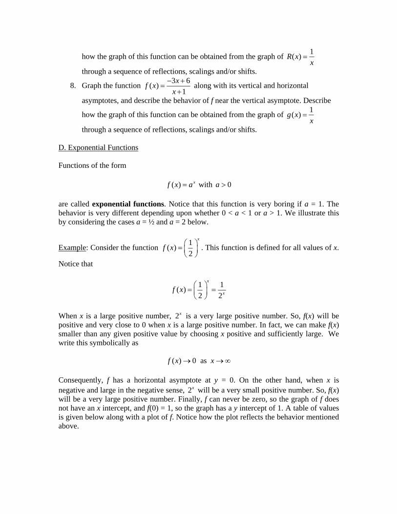
Example: Consider the function 1( )2

x

f x ⎛ ⎞= ⎜ ⎟⎝ ⎠

. This function is defined for all values of x.

Notice that

1 1( )2 2

x

xf x ⎛ ⎞= =⎜ ⎟⎝ ⎠

When x is a large positive number, 2x is a very large positive number. So, f(x) will be positive and very close to 0 when x is a large positive number. In fact, we can make f(x) smaller than any given positive value by choosing x positive and sufficiently large. We write this symbolically as

( ) 0 as f x x→ →∞ Consequently, f has a horizontal asymptote at y = 0. On the other hand, when x is negative and large in the negative sense, 2x will be a very small positive number. So, f(x) will be a very large positive number. Finally, f can never be zero, so the graph of f does not have an x intercept, and f(0) = 1, so the graph has a y intercept of 1. A table of values is given below along with a plot of f. Notice how the plot reflects the behavior mentioned above.

x f(x) -3.5 11.3137-3 8

-2.5 5.65685-2 4

-1.5 2.82843-1 2

-0.5 1.414210 1

0.5 0.707111 0.5

1.5 0.353552 0.25

2.5 0.176783 0.125

3.5 0.088394 0.0625

0

2

4

6

8

10

12

14

16

18

-6 -4 -2 0 2 4 6

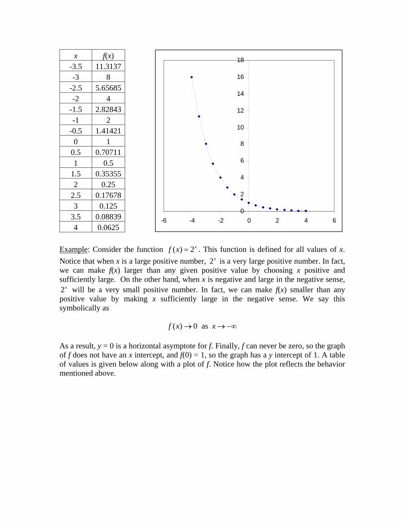
Example: Consider the function ( ) 2xf x = . This function is defined for all values of x. Notice that when x is a large positive number, 2x is a very large positive number. In fact, we can make f(x) larger than any given positive value by choosing x positive and sufficiently large. On the other hand, when x is negative and large in the negative sense, 2x will be a very small positive number. In fact, we can make f(x) smaller than any positive value by making x sufficiently large in the negative sense. We say this symbolically as

( ) 0 as f x x→ →−∞ As a result, y = 0 is a horizontal asymptote for f. Finally, f can never be zero, so the graph of f does not have an x intercept, and f(0) = 1, so the graph has a y intercept of 1. A table of values is given below along with a plot of f. Notice how the plot reflects the behavior mentioned above.

x f(x) -4 0.0625

-3.5 0.08839-3 0.125

-2.5 0.17678-2 0.25

-1.5 0.35355-1 0.5

-0.5 0.707110 1

0.5 1.414211 2

1.5 2.828432 4

2.5 5.656853 8

3.5 11.31374 16

0

2

4

6

8

10

12

14

16

18

-6 -4 -2 0 2 4 6

In general, the graphs of ( ) xf x a= for 0a > and 0a ≠ are similar to those for

1( )2

x

f x ⎛ ⎞= ⎜ ⎟⎝ ⎠

and ( ) 2xf x = given above. The plots are shown in the figures below.

( ) xf x a= for 0 < a < 1 ( ) xf x a= for a > 1

Example: We can use the information above to graph the function ( ) 2xf x = − . The graph of f is the reflection of the graph of ( ) 2xg x = across the x axis.

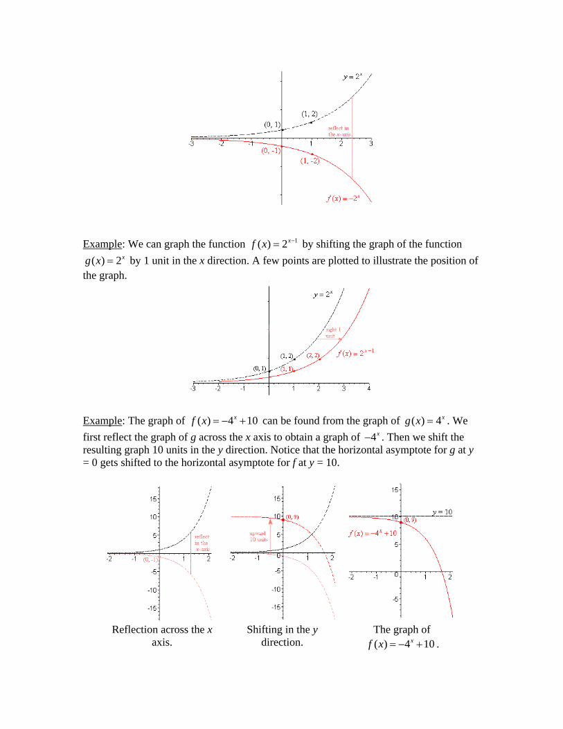
Example: We can graph the function 1( ) 2xf x −= by shifting the graph of the function

( ) 2xg x = by 1 unit in the x direction. A few points are plotted to illustrate the position of the graph.

Example: The graph of ( ) 4 10xf x = − + can be found from the graph of ( ) 4xg x = . We first reflect the graph of g across the x axis to obtain a graph of 4x− . Then we shift the resulting graph 10 units in the y direction. Notice that the horizontal asymptote for g at y = 0 gets shifted to the horizontal asymptote for f at y = 10.

Reflection across the x axis.

Shifting in the y direction.

The graph of ( ) 4 10xf x = − + .

Example: The graph of 1( ) 2 6xg x += − can be given from the graph of ( ) 2xg x = . We start by shifting the graph of ( ) 2xg x = by -1 unit in the x direction. Then we shift the result -6 units in the y direction. Notice that this process shifts the horizontal asymptote for ( ) 2xg x = at y = 0 to the horizontal asymptote for g at y = -6.

Shifting -1 units in the x

direction. Shifting -6 units in the y

direction. The graph of

1( ) 2 6xg x += − . Exercises:

1. Give the horizontal asymptote and the y intercept for the graph of ( ) 2 3xg x = − .

2. Explain why the graph of 1( )3

x

f x−

⎛ ⎞= ⎜ ⎟⎝ ⎠

is the same as the graph of ( ) 3xf x = .

3. Give the horizontal asymptote and the y intercept for the graph of 1( ) 54

x

f x−

⎛ ⎞= +⎜ ⎟⎝ ⎠

.

4. Explain how to use horizontal and vertical shifts to obtain the graph of ( ) 2 3xg x = − from the graph of ( ) 2xf x = .

5. Explain how to use horizontal and vertical shifts to obtain the graph of 31( ) 7

3

x

g x+

⎛ ⎞= −⎜ ⎟⎝ ⎠

from the graph of 1( )3

x

f x ⎛ ⎞= ⎜ ⎟⎝ ⎠

.

6. Explain how to use horizontal and vertical shifts to obtain the graph of 2( ) 5 1xg x = − from the graph of ( ) 25xf x = . Hint: ( )cbc ba a= when a > 0.

7. Graph ( ) 2 3xg x = − .

8. Graph 31( ) 7

3

x

g x+

⎛ ⎞= −⎜ ⎟⎝ ⎠

.

9. Graph 33( ) 2

2

x

g x+

⎛ ⎞= +⎜ ⎟⎝ ⎠

.

E. The Number e, Radioactive Decay, and Savings Accounts

There is a positive number which is referred to as the natural exponent, and the number is so well known that it is given the special name e. The number e is an irrational number, so its exact value is not known. However, it can be approximated to many decimal places. In fact, rounded to 20 decimal places, e is given by

2.7182818284590452354e ≈

There are a number of websites which give e to more decimal places. For example, you a quick search will return e rounded to 200 decimal places as

2e ≈ .71828182845904523536028747135266249775724709369995957496696762 7724076630353547594571382178525166427427466391932003059921 81741359662904357290033429526059563073813232862794349076 32338298807531952510190 The reason that e is referred to as the natural exponent is because it shows up in so many important applications. Since e > 1, the graph of the exponential function ( ) xf x e= is very similar to those given in the section above. We show this graph below.

The techniques from the previous section can also be used to graph ( ) xf x e−= since

1 xxe

e− ⎛ ⎞= ⎜ ⎟

⎝ ⎠ and 0 < 1/e < 1.

Example: Experimental evidence has shown that radioactive substances decay in a such a way that the amount A(t) of the substance present at time 0t ≥ (in years) is given by

( ) ktA t Ce−= , where k is a positive constant. Notice that ( )0 0(0) kA Ce Ce C−= = = since 0 1e = . Consequently, the formula for A(t) can be rewritten in the form

( )( ) 0 ktA t A e−= for 0t ≥ .

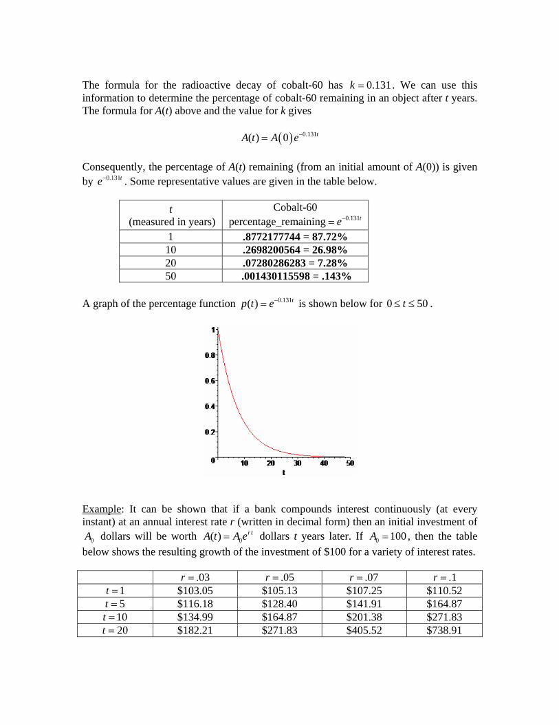
The formula for the radioactive decay of cobalt-60 has 0.131k = . We can use this information to determine the percentage of cobalt-60 remaining in an object after t years. The formula for A(t) above and the value for k gives

( ) 0.131( ) 0 tA t A e−=

Consequently, the percentage of A(t) remaining (from an initial amount of A(0)) is given by 0.131te− . Some representative values are given in the table below.

t (measured in years)

Cobalt-60 0.131percentage_remaining te−=

1 .8772177744 = 87.72% 10 .2698200564 = 26.98% 20 .07280286283 = 7.28% 50 .001430115598 = .143%

A graph of the percentage function 0.131( ) tp t e−= is shown below for 0 50t≤ ≤ .

Example: It can be shown that if a bank compounds interest continuously (at every instant) at an annual interest rate r (written in decimal form) then an initial investment of

0A dollars will be worth 0( ) r tA t A e= dollars t years later. If 0 100A = , then the table below shows the resulting growth of the investment of $100 for a variety of interest rates.

.03r = .05r = .07r = .1r = 1t = $103.05 $105.13 $107.25 $110.52 5t = $116.18 $128.40 $141.91 $164.87

10t = $134.99 $164.87 $201.38 $271.83 20t = $182.21 $271.83 $405.52 $738.91

Exercises: 1. Graph the function ( ) 1tp t e= + . 2. Graph the function ( ) 2tg t e−= + . 3. Graph the function 0.21( ) 100 tf t e= . 4. A certain radioactive substance has a k value given by 0.015k = . Create a table

showing the percentage decrease in the substance for t = 1, 10, 50, 100, 500 years. 5. A certain radioactive substance has a k value given by 0.0045k = . Create a table

showing the percentage decrease in the substance for t = 1, 10, 50, 100, 500 years. 6. A certain radioactive substance has a k value given by 0.015k = . Estimate the ½

life of this radioactive substance. That is, estimate the time that must pass before 50% of the substance decays.

7. $1000 is invested in an account that compounds interest continuously at a rate of 8%. How much money will be in the account after 10 years?

8. Your great great grandfather started a savings account 100 years ago with $100. Give an estimate for the amount of money currently in the account assuming the annual interest rate on the account has averaged 7% compounded continuously.