Nonlinear Bifurcations to Time-dependent' Rayleigh-Benard Convection

J. M. LopezA and J. O. MurphyB

A Aerodynamics Division, Aeronautical Research Laboratories, Port Melbourne, Vic. 3207, Australia. B Department of Mathematics, Monash University, Clayton, Vic. 3168, Australia.

Abstract

Aust. J. Phys., 1988,41,63-82

The single-mode equations of Boussinesq thermal convection have been extended to include a toroidal component of velocity and hence the associated vertical component of vorticity. This formulation allows, under certain determined conditions, the purely poloidal solutions to become unstable to toroidal perturbations via symmetry breaking bifurcations. The bifurcation sequences are governed by a three parameter family: the aspect ratio of the convection cell, the Prandtl number of the fluid and the Rayleigh number of the flow. The initial growth of the vertical vorticity has been found always to be steady. However, in certain parameter ranges there are transitions leading to time-dependent behaviour via a Hopf bifurcation which may be in the form of symmetrical oscillations, asymmetrical oscillations, doubly-periodic behaviour or, possibly, chaos, depending on the form of the transient poloidal phase of the evolution.

1. Introduction

Although theoretical studies and experimental investigations of Rayleigh-Benard convection have attracted considerable attention over recent years, resulting in a concise picture of the onset of the various instabilities, there are still many unresolved and significant features of the time-dependent regime of cellular convection. Thermal convection has no mean flow with all motion being due to the growth of disturbances to finite amplitude. This, together with the existence of a regime of laminar flow which separates the static conductive and turbulent convective regimes, provides an ideal situation in which to study the transition to turbulence.

The linear theory offers no information concerning the time-dependent nature or character of the finite-amplitude disturbance. It only specifies that, in the absence of external influences, the disturbances have a real growth rate (Chandrasekhar 1961) and that the value of this growth rate depends solely on the horizontal wave number of the disturbances and the Rayleigh number. If the growth rate is positive, the disturbances will grow to finite amplitude and continue to grow exponentially until the coupling nonlinear terms become significant and halt their growth. In order to follow the time-dependent evolution of the disturbances through to finite amplitude, the nonlinear equations have to be solved.

Any analytical nonlinear study of time-dependent convection at high Rayleigh number is intrinsically difficult, even over restricted parameter ranges. Most analytic work undertaken so far has principally been either of the form of asymptotic expansions, where extreme values of the parameters have been used in order that

0004-9506/88/010063$03.00

64 J. M. Lopez and J. O. Murphy

certain nonlinear terms may be ignored, or by perturbation methods. In this case, the variables are normally expanded in terms of the amplitude of the convective disturbance, which is assumed to be small, and consequently, the analysis is valid only near the critical stability state. Hence, as a result of the inherent difficulties associated with obtainir.g analytical solutions there has been a significant trend towards the numerical study and simulation of nonlinear Rayleigh-Benard convection.

Full three-dimensional simulations of Rayleigh-Benard convection in a box are. now available for Rayleigh numbers up to 3·8 x lOs (Grotzbach 1982). Qualitative agreement with the gross features of laboratory experiments in small boxes is achieved, however the complex pictures presented do not readily allow for the identification of the mechanisms involved in the evolution and structure of the flow. The limited horizontal extent of the computational domain imposed by the available numerical resolution renders such computations incapable of simulating convective layers oflarge or infinite extent which are predominant in astrophysical and geophysical situations. The use of simpler models remains important because of their ability to simulate large horizontal domains, and to isolate and identify particular features and the mechanisms present in the evolution of the flow.

One of the most common approximations used is to assume the flow to be two-dimensional. Recently, Bolton and Busse (1985) have shown that convective rolls are unstable to three-dimensional perturbations outside a small region of parameter space in the neighbourhood of the critical state.

Three-dimensional convection has been simulated by axisymmetric convection (Jones et al. 1976) with stress-free boundaries. However, as a consequence of the imposed special symmetry together with the use of a purely poloidal velocity field, 'interial' convection sets in at low Prandtl and high Rayleigh numbers leading to solutions which have speeds far greater than the reduced free-fall speed. These authors have found (Jones and Moore 1979) that these solutions are unstable and would probably be limited by more general three-dimensional behaviour. A further drawback to axisymmetric ·convection is that it can only simulate an isolated cell, whereas in observed convective phenomena, cells interact with and are influenced by neighbouring cells.

An effective approximation technique used to simulate three-dimensional convection involves the use of series expansions where the horizontal dependence is averaged out, whilst still retaining its cellular signature through certain parameters. The expansions are then truncated to retain a finite number of horizontal modes. This technique has come to be known as the modal expansion method. Its most common use has been in the form of the single-mode approximation, where only the leading term in each of the expansions has been retained involving only a single wave number. In the past, applications of the single-mode approximation (e.g. Roberts 1966; Toomre et al. 1977) have always evolved to a steady state. This has led a number of authors (e.g. Marcus 1981; McLaughlin and Orszag 1982; Schubert and Strauss 1982; Toomre et al. 1982) to suggest that the single-mode model is incapable of demonstrating any non-steady time dependence, and attributed this inadequacy to the severity of the truncation. This line of reasoning was further encouraged by the appearance of time-dependent solutions when higher modes were included in the expansions (Toomre et al. 1982). However, as demonstrated in this present study, it was not the severity of the truncation which suppressed time-dependent behaviour, but the omission of vertical vorticity from the model.

Nonlinear Bifurcations 65

In all previous studies of the Rayleigh-Benard problem using the modal approach, a particular solution of the continuity equation (\1. u = 0) for the velocity had been adopted in which the vertical vorticity was identically zero. Busse (1972) pointed out that it would be surprising if the dynamics of convection lacked the additional degree of freedom which the vertical component of vorticity provides. Here, a more general solution incorporating a toroidal component of velocity is implemented which allows for a nonzero component of vertical vorticity. It is shown that the addition of this extra degree of freedom to the single-mode equations permits non-steady time-dependent solutions within a range of parameter values which agree with experiments on time-dependent convection (Krishnamurti 1973).

An association between vertical vorticity and time-dependent behaviour (finite oscillations) was established by Busse (1972) when he demonstrated that, for stress­free boundaries in the limit of small Prandtl number, the 'oscillatory' instability sets in at the same time as the vertical component of vorticity is generated. In a modification to the perturbation expansion method of Busse (1972), Manneville and Piquemal (1983) found that for stress-free boundaries, in the limit of infinite wavelength, some vertical vorticity is present and that in addition to the 'convective' mode, there is also an additional 'vertical vorticity' mode which is associated with the oscillatory instability. In their review article on experimental reports, Libchaber and Maurer (1981) noted that before the onset of the oscillatory instability, the vorticity field is essentially horizontal, and that a vertical component of the vorticity is apparently introduced by this instability. They found that the presence of a vertical vorticity component may establish a time-dependent motion of the convective structure. Willis and Deardorff (1970), in their experimental investigation of the Rayleigh-Benard problem, commented on the need to invoke a vertical component of vorticity in any mathematical simulation of the velocity field in order to reproduce the oscillations and permit an understanding of the velocity structure which they observed. It is found from both finite-amplitude expansions and experimental observations that there is a strong association between vertical vorticity and time-dependent behaviour. However, as noted by Busse (1978): 'The influence of the vertical component of vorticity on the nonlinear properties of convection is not well understood.'

Surprisingly, there have been relatively few numerical investigations in which the vertical vorticity has been incorporated. Lipps (1976) in reference to his three-dimensional model agreed with Busse (1972) that oscillatory behaviour and the generation of vertical vorticity go hand-in-hand, but said little else about the velocity structure of his solutions. In the two-dimensional roll models, the vorticity is of the form (0, cu, 0) and accordingly the vertical vorticity is zero by definition. The same is also true of the axisymmetric models. The numerical model used here incorporates an explicit component of vertical vorticity; one which is not induced by external influences such as rotation, magnetic fields or shear flows. The effects of the vertical vorticity on the steady-state system were studied in detail by Murphy and Lopez (1984) and Lopez and Murphy (1984), and in the present paper its effect on the time-dependent nature and evolution of the system is investigated.

2. Eqnationg

The Rayleigh-Benard problem describes the convective transport of heat through a layer of Boussinesq fluid with coefficient of volume expansion a, viscosity J.A"

conductivity K, specific heat at constant volume Cv and depth d, which is held

66 J. M. Lopez and J. O. Murphy

between two horizontal isothermal boundaries maintained at a temperature difference of fJ. T. The physics of the problem is described by the following four basic equations (Chandrasekhar 1961):

P = PoP -a(T -To)}, (1)

where the density P has a mean value of Po when the temperature has a mean value of To;

\7.u=o;

ou 2 P - +pu.\7u+\7P-pG-JL\7 u = 0; ot

oT 2 pCv - +pCv u. \7T -K\7 T = o. ot

(2)

(3)

(4)

When these equations are linearised, they allow a separation of the horizontal variables (x,y) from the vertical variable z (Chandrasekhar 1961). For cellular convection, the horizontal dependence of the vertical component of velocity and the temperature are described by any function f(x, y) which satisfies the two-dimensional Helmholtz equation

2 2 o f(x, y) 0 f(x, y) ---+---

ox2 oy2 -k2f(x,y). (5)

k being the horizontal wave number. In adopting the modal approximation for the nonlinear problem, the variables are

expanded in a series of the linear eigenfunctions f(x, y) satisfying (5). With the single-mode approximation, only the leading term in the expansion is retained and the temperature is expanded in the following manner:

T = To(z, t) + F(z, t)f(x, y), (6)

with similar expressions for pressure and density. Any expansion adopted for the velocity must also satisfy the continuity equation

(2). The usual component form is

u = {~2 D W(z, t) of ox'

1 k2 D W(z, t)of

oy' W(z, t)l}, (7)

as specified by Gough et al. (1975) and Toomre et al. (1977, 1982), where D = %z. However, this particular poloidal solution of (2) imposes a severe physical constraint on the system, in as much that the vertical component of vorticity is identically zero.

An alternative more general solution of (2) is now employed which allows the system an additional degree of freedom by adding a toroidal component to the velocity field (Ehrenzweig 1969), with

Nonlinear Bifurcations

{ I ( af af ) 1 ( af af ) u = 2" DW(z, t)- +Z(z, t)- '2" DW(z, t)- -Z(z, t)- , k ax ay k ay ax

The associated vorticity field is now

" { 1 ( af 2 2 af) v X u = w = k 2 DZ(z, t) ax -(D - k ) W(z, t) ay ,

67

W(z, t)f}.

(8)

;2(DZ(Z,t):~ +(D2_k2)W(Z,t):~), Z(Z,t)f}. (9)

Here the horizontal components of vorticity are modified by the nonzero vertical vorticity Z(z, t), whose solution is given by the basic modal equations which follow from this formulation.

The non-dimensional form of the single-mode equations, obtained from a variational principle following the derivations by Van der Borght and Murphy (1973), which employs the following scalings-Iength scaled by the vertical depth d, velocity by K/ d, where K is the thermal diifusivity, temperature by A T and time by d 2/K-are

a(D2 - a2) W = a-(D2 _ a2)2 W _ a-Ra2 F at

-C{ WD(D2_a2)W+2(D2_a2)WDW+3ZDZ} , (10)

az = a-(D2-a2)Z-C(WDZ-ZDW), (11) at

aF 2 2 - =(D -a)F-WDTo-C(2WDF+FDW), (12) at

aTo 2 - = D To-D(F W), (13) at

where the Rayleigh number R = gad3 AT /KV, the Prandtl number a- = V/K, v being the kinematic viscosity, and a = kd is the aspect ratio of the convection cell. The interaction constant

c = ! II f3 dXdY / II f2 dxdy cell cell

feeds the signature of the horizontal dependence through to the horizontally averaged system.

Two important derived quantities characterise the convective flow. The first of these is the NusseIt number N. For a steady-state system, it is defined as the first integral of the steady form of (13), that is

N = F(z) W(z) -DTo(z). (14)

In this case N establishes a non-dimensional form of the total heat flux through the layer and is independent of z. For non-steady solutions, however, a time average of

68 J. M. Lopez and J. O. Murphy

(14) is required for N to be independent of z. When time-periodic solutions arise, an average over one period ensures this independence. However, for non-periodic and especially intermittent solutions, long time averages are required, where the definition of 'long' is not precise. Accordingly, the Nusselt number as defined by (14) becomes a function of time.

The second important derived quantity is the mean helicity, which is only nonzero if the flow has a vertical component of vorticity, and this is defined by

By = f f fcell u.(\lx u)dxdydz,

which in this case takes the form

By = f:IDW(Z, t)DZ(z, t)-Z(z, t)(D2-a2)W(z, t)

+ a2 W(z, t) Z(z, t)} dz.

(15)

(16)

Clearly, the mean helicity is not a consequence of any external rotation of the system or imposed shear. flow as is usually the case with systems which possess a nonzero mean helicity.

The planform f(x, y) in which to expand the variables needs to be determined. It should establish motions which are cellular, and this condition is equivalent to specifying that the solutions be doubly periodic in x and y. There are four basic 'shapes' or planforms which satisfy this requirement. The 'cellular' solutions which define a roll, triangle, and rectangle, of which the square is a particular form, have C = 0 and consequently do not interact with one another, contrary to what one would expect from physical flows. The interaction parameter C takes a nonzero value for the hexagonal form of f(x, y) which in tum has a number of consequences. Clearly, a number of nonlinear terms are retained in the system (10)-(13), resulting in substantial nonlinear couplings between the velocity and temperature fields, as well as the nonlinear advection terms. Also, if C = 0, the equation for the vertical component of vorticity is completely decoupled from the system, with a trivial solution resulting for classical boundary conditions. The system with C = 0 is known as the 'mean-field' equations for which only steady-state solutions exist (Herring 1963), and is independent of the Prandtl number. Consequently, in adopting the modal approximation to simulate the Rayleigh-Benard problem realistically, the hexagonal planform should be used.

The form of f(x, y) which describes a hexagonal planform is due to Christopherson (1940):

f(x,y) = (j)i{2 cos(yI~ kx) cos(!ky) + cos(ky)} , (17)

for which the interaction constant C = yl3/2. To establieh our results, each time evolution was started from random perturbations

of the order 10-6, introduced at each z grid point, simulating the amplification of disturbances from small random fluctuations to finite amplitUde. The standard stress­free boundary conditions have been imposed with W = D2 W = D Z = F = 0 at z = 0 and 1, and To = 0 at z = 0 and To = - 1 at z = 1.

Nonlinear Bifurcations 69

3. Numerical Method

The system (10)-(13) has been solved using finite differencing. Both a second-order central-difference Crank-Nicolson method and a second-order backward-difference scheme were employed with no apparent difference in the results between the two numerical methods being found. The band-matrix which results from these methods was solved using an efficient band-matrix algorithm which had been developed specifically for systems of second-order equations (Van der Borght 1980).

The solutions, especially at extreme, values of the parameters, develop very harrow boundary layers which in turn require a large number of grid points to be adequately resolved in the vertical direction. This problem was alleviated by using a non-uniform grid which has the effect of stretching the boundary layer regions and contracting the central regions. The stretching function utilised is of the form

z(~) = exp[-{(1-A)/</>Jn]-exp[-{(I-A-~)/</>Jn], exp [- {(1-A)/</> J n]_ exp [_(A/</»n]

with typical parameter values n = 4, A = 1·05 and </> = 0·6.

4. Results

(18)

The extra degree of freedom given to the system by the inclusion of the vertica1 component of vorticity has led to the existence of nonlinear bifurcations to time­dependent states. One of the mechanisms producing time dependence in Rayleigh­Benard convection has now been identified and some of the resulting forms are now analysed. '.

Regardless of the final state ofthe evolution-steady, periodic or non-periodic-the initial evolution of the system always follows the same pattern when the configuration at t = 0 consists of small random perturbations. This initial stage of evolution from the conductive state is clearly determined by the linear terms in (10)-(13). The growth rate of the initial disturbances is in fact the linear growth rate, and it is well known (Chandrasekhar 1961) that this growth rate is always real, and hence leads to a simple bifurcation from the conductive state when the growth rate is positive. At this stage the linear terms in (11), which are not affected by buoyancy forces, have trivial solutions, and any perturbations in Z will decay. The vertical velocity, along with the other disturbances, will continue to grow until its amplitude reaches a value where the nonlinear terms become important. The nonlinear terms in (10), (12) and (13) then halt the exponential growth, and depending on the value of the Rayleigh number, Prandtl number and the aspect ratio, the vertical vorticity acquires a real growth rate via the nonlinear terms in (11). If this growth rate is negative or zero, the

. system continues to convect in what is termed a steady type I state with zero vertical vorticity. However, if it is positive, the vertical vorticity will grow exponentially until it becomes dynamically significant, leading to type II solutions. Then, through the nonlinear couplings in (10) and (11) between the vertical vorticity and the vertical velocity, there is a transfer of kinetic energy from the 'convective' motions (typical of type I) to the 'cyclonic' motions (typical of type II), which leads to a substantial decrease in the vertical velocity and convective heat transported as. measured by the Nusselt number. For some parameter values, a simple equilibrium is reached b~tween

70 J. M. Lopez and J. O. Murphy

the vertical velocity and the vertical vorticity and the system settles down to a type II steady state. However, for other parameter values, the nonlinear couplings lead to a non-steady time-dependent state, and it is this state with which this paper is primarily concerned.

The first bifurcation, namely that from the conductive state to steady type I, is independent of the Prandtl number and its onset depends only on the Rayleigh number and the aspect ratio of the cell; in fact it is described by the marginal stability curve from the linear theory (Chandrasekhar 1961) which is well understood. In the vicinity of this bifurcation,perturbation methods are useful for investigating this weakly nonlinear regime.

The onset of one form of the second bifurcation, the transition from type I to type II steady motion in which there is a nonzero vertical component of vorticity, is more difficult to pinpoint in parameter space as it depends not only on the Rayleigh number and the aspect ratio, but also on the Prandtl number. Its onset is governed by the nonlinear terms in (10)-(13), rather than the linear terms as is the case for the first bifurcation. The only simplifying factor is that this state is also associated with the time-independent form of the equations, and has in fact been studied earlier (Murphy and Lopez 1984). It was observed that when a = 7r, an approximate relationship of the form R - 103 (1"1.5 gives the locus of points at which the second bifurcation takes place. The dependence of the onset of type II steady-state solutions on the aspect ratio has been the subject of another earlier study (Lopez and Murphy 1984). The apparent non-uniqueness disclosed in those earlier studies of the time-independent system has now been resolved.

An example of the nonlinear bifurcation is given in Fig. 1 where the time evolution of the profiles of (a) W(z, t), (b) Z(z, t) and (c) l'o(z, t) are plotted in the stretch coordinate~. If we focus on the vertical velocity profiles for W(z, t) in Fig. 1, the expected characteristic growth of the initial instability is observed to take place, with the actual rate depending on the nominated values of Rand a. A small degree of overshooting is typically associated with the conclusion of this transient phase for W(z, t) which is followed by a quasi-steady state with no time variation in W.

During the corresponding time interval for the growth of the vertical velocity, the vertical vorticity actually decays and would continue to do so when essentially large (1"

values and values of a in the upper part of the range of wave numbers which support convection for a particular Rayleigh number are involved, resulting in a stable type I solution. Growth of Z(z, t) on a characteristic time scale only takes place after the growth of W(z, t) has ceased.

The steady profile resulting from the type I solution for W(z) can be represented by

M

W(z) = 1: wn sin(mTz), n=1

which satisfies the free boundary conditions W = D2 W = 0 at z = 0 and 1. We now assume that

Z(z, t) = y(z) exp(pt) ,

and introduce both these expressions into (11) which, after the elimination of exp(pt),

o

o

(0)

Tim

e eV

olut

ion

of

(0)

/p(

~ (b

\ Z

,

z".

z (z

. ,)

""d

(e)

ZO

(z")

Plo

tted

in "

''''

'''l

eb

_

.. , cr.. _

0

4

~ or.

l' -

1 ,

(r ~

1·0

an

d a

2 ~

10.

Fig

. 1.

(b)

(c)

72 J. M. Lopez and J. O. Murphy

leads to

d2y C( M • )dY (p C7T M ) -2 - - l: Wn sm(n7TZ) - - - +t? - - l: wn n cos(n7Tz) Y = O. (19) dz (T n=l dz (T (T n=l

Along with the boundary conditions dy/dz = 0 at z = 0 and 1 which follow from DZ(z, t) = 0 at z = 0 and 1 for free boundaries, equation (19) represents an eigenvalue problem for the characteristic growth of Z(z, t). If we utilise a finite difference representation of this equation along with an iterative scheme, based on the false poSition method, the set of eigenvalues p for nominated parameter values is then established. Although this differential equation appears to have no explicit dependence on the Rayleigh number, the coefficients wn depend implicitly on it.

100000

90000

80000

10000

60000 R

50000

'iODOO

30000

20000

10000 2 3 'i 5 6 7 8 9 10

a

Fig. 2. Contour diagram establishing the computed characteristic growth rate of the vertical component of vorticity p from equation (19) in the R-a plane for free boundaries and CT = 1· O. Continuous curves designate a positive growth rate leading to type II solutions, and the broken curves indicate that for these R and a values the initial perturbations decay and Z( t) "'" 0, i.e. type I solutions. The contour line labelled 0 is the locus of the type II bifurcation in R-a parameter space.

The numerical results for p, when (T = 1, are given in R-a parameter space in Fig. 2. The zero level contour in this diagram is the demarcation line which separates the type I and II solutions and is in excellent agreement with the type of solution obtained independently from the time integrations of (10)-(13). Moreover, the location of this contour confirms that type II solutions cannot become established in narrow

Nonlinear Bifurcations 73

cells where the closeness of the side walls would inhibit the characteristic swirling motions. Specifically, from the linear stability theory (Chandrasekhar 1961), the range of wave numbers that supports cellular convection at R = 104 is O· 3 < a < 9.2, while Fig. 2 shows that p > 0 only if a < 5 ·0. It is also of interest to note that the contours for p > 0 exhibit a definite R-a minimum and further, they parallel the corresponding direct instability curve for the onset of stationary convection. For a particular horizontal wave number the growth rate of the vertical component of vorticity increases with R which in tum determines the degree of convective instability in the fluid.

In the next identifiable phase, which is associated with the continued growth of the vertical component of vorticity at a rate determined by the value of p, the nonlinear term -3CZ(z, t)DZ(z, t) in (10) becomes significant and the effect of this coupling term iS,manifested bya reduction in W(z, t), which also appears to have a characteristic decay rate. Subsequently, a balance is attained where both Z(z, t) and W(z, t) show no further changes and a stable type II convective state is attained,

Overall the time dependence of N follows that of W(z, t) and a feature of particular physical interest is the resultant drop in the convective heat transport which occurs following the growth of Z(z, t).

5. Discussion

In the preceding section, the presentation was restricted to cases where the nonlinear bifurcation led to a final steady state, referred to as a type II steady state. However, the numerical integrations of (10)-(13) have also revealed an intricate bifurcation sequence as the control parameters R, (T and a are varied.

The growth rate, p, of Z has always been found to be real, leading to a simple bifurcation. However, once the - 3 C ZD Z term in (10) has grown large enough, it not only reduces the amplitude of the W profile, but also alters its shape. At this stage, the linear equation (19) no longer bears any direct relevance to the system (10)-(13) as W is no longer constant. The manner in which the nonlinear terms interact in the system (10)-(13) then determines whether a steady type II or a time-dependent type II state is reached. This identifies a first step towards time-dependent convection.

A small selection of the many numerical time integrations of (10)-(13) which have been performed (Lopez 1985) are given in Figs 3-6 where time series of the maximums of W(z, t) and Z(z, t) as well as the mean helicity and Nusselt number have been plotted, along with the corresponding evolutionary trajectories illustrating the phasing between W max and Z max and between Hv and N. These examples illustrate some of the possible time-dependent properties of the type II state. In Fig. 3, for R = 105,

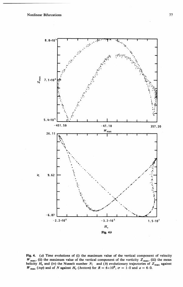
(T = 1·0 and a = 1.0, a symmetric oscillator is the final state of evolution, whereas in Fig. 4, for R = 6x 106, (T = 1·0 and a = 6·0, an asymmetric oscillator results. Doubly-periodic behaviour results for R = lOs, (T = O· 5 and a = 1·0 as illustrated in Fig. 5, and for larger R = 2 x 108 , (T = 1,0 and a = 3·0, more complicated oscillations are found as in Fig. 6.

It is well known from the many previous studies of Rayleigh-Benard convection with a purely poloidal velocity field that the profiles of the solution variables change character in different parameter regimes. For example, when a is large, the W(z) profile is nearly constant across the interior of the layer with very thin boundary layers adjusting the vertical velocity to zero at the boundaries, and when a is small

74 J. M. Lopez and J. O. Murphy

n.51E.~ ~~~~~-'---r--r-~--.--,---.--r--.--,--'r--r--.--.--'---r--r--'

" ~ O.lZE.~

.0 ... 7E.OZ L' __ ~-L'L' __ -L __ ~ __ L--J __ -L __ -L __ ~ __ L--J __ -L __ -L __ L-~L-~ __ -L __ ~ __ L--J

0.00 1.60 3.bO 5.~O 7 ... 0 O. ZZE.03 r' -r-""T-.--r-.--.-.---;-,----,-...,--r-""T-r--r-.,.---,--.,----,.---o

~ e 0.11E.03

N

O. S2F.--06 L. _.LI'LL---1_...L---1_...L---1_...L---lL---L_L---L_L--L_L-.-L_..l..----l_....L........J

0.00 1. dO 3.bO 5.40 7 ... 0 O.l3E.OS r.--_r~._rl--_r--_r--_r--_r--_r--_r--_.--_.--_.--_.--_.--_.--_.--_.--_,--_,--_,r__,

~ -0.l7E-04

.0. lBE .05 '----' __ .c' .J..I __ ~ __ -"-__ '--.....l __ -L __ -L __ ..L _-'-__ --'-__ -"-__ "----''--.....l. __ ...L __ ..L __ L---l __ ...J

0.00 1.60 3.bO 5.40 7 ... 0 4.54 r,--~--~~r-~---r--~--~~r-~---r~---r--._--~-,r-_.---r--._--T__,

~ Z.59

O.b4 [, -L~~~LLL-L--L...-L.....L---1..---1.---l~L....L---1--.....l---L-----L.~ 0.00 1.60 :.bO

Time

Fig.3a

5.40 7.t1l

Nonlinear Bifurcations

1 90 I . :c::::::==;:::; _ I ::;:l ..........

g 160 N

, I .\. J \ .

. \. \ . \. I \ . . ~ J \ I .\\ I

. . 0' 130

-10.33

1. 59

~ 1. 25

T .\ ~

.-, \ "\:

.'\ , ': ..

~

\ \ ,

\ \

\ \

\ ~

\ \ \\

l.. \

~ \ ,

-0.13

t .. '\. l

~

.. \.. ./ .. I . -\ l

\ . f· .. \ . .J \./ .. . .\ .

7 /

I / ,

/

10.07

j.

t i.

.; I

{. ! ~

i i /

/ / ~

( I ,.

f /

~.

-l ~ .I

:; ./

'\

i /

i / I. ,

/'

0.81 -5700 - 87 5500

Hv

Fig.3b

75

Fig. 3. (0) Time evolutions of (i) the maximum value of the vertical component of velocity W max. (ii) the maximum value of the vertical component of the vorticity Zmax. (iii) the mean helicity Hy and (iv) the Nusselt number N; and (b) evolutionary trajectories of Zmax against W max (top) and of N against Hy (bottom) for R = 105• (T = 1·0 and 0 = 1· o.

<t'

... ...

... "

'J

J ~

>.

Ie::!:

'" C

'l <!:.

a c:i

..<:: fr

c:: -

;:I

l c::

-<

I-

-ci

c::: <::

§ ~ ...;

c:::

"0

c:::: <::

c:: =--

os N

~

~

~

~

<1) I-

:.. 0

. <::

a Q

~

cO c:i

0

~

...J '-

-~

<:

...; <

:

c::: ?~

:-==

~

o::r <

: <1)

~

'~

'J

~

'oJ

~ -

-c::

ciI co

a c:i

c, S

-c::

<:

--

~

-c:

-~

~

l w

cD

j ~

~

-C

" C

" I-

-a

0 (:>

0 -

:r

-l-

t -

, , , , l'l , , ,

c 0

, , a

'" C

" co

C"

co 0'

0' ")

0'"

...

0 o~

CD o~

N

9 0

0 <i

c.: '"

'i? 'i?

0 'i?

c.: 'i:

. •

, w

.. ,

1..;.: w

'"'

w

.. , .. ,

~

.. , .. ,

.. , <D

".::

e-N

.0

'"

... ~

CD ...

22 '"

.0

cr <

t' e

'T)

., IF

'J

0 a

<;' a

a cO

a <;'

<;' a

a <;'

~

XB

WAi

XB

WZ

r-

AH N

Nonlinear Bifurcations

N~

~

8. 8x10 ~I ,.J ..... c·t!C .• ! ..... • :°:.1° 0° • "~'). •

. :,'

....... .. '

.:.' ".:"it ; ... ,

.'\. : .... ; ... ..

'~ .:. ~.~;:. ?".:.,~ .: ... ~ .• ~. '::!.

. : '.

,.' ". :.0

..... ".

.:0'

.~' . I :-

I:. .r'

• r.":'·· . :;

i.":'"

-:-..... .......

oOso .... ,,',

:;' .

0.1'0;_ " . ....• : ::.;.

." ..~

:°trt;,

'\; .. ~, • .0:.

t.:" "0;:":

\ "~~~i

5.4x10~LI __ ~I~'~~ ____ ~ __ -L __ ~ ____ L-__ ~ __ ~ ____ ~~~

-451.59

26.11 'r. ~\ ~ .. "" ~ ....

":1

'"

9.62

-6.87

-2.2x10 6

-0"" ':, -"".

-:0 ~.

. ,

l:

-47.18

'.

'. '0,. ,

., . ".". ~. ~

Of::

":~ .,,,-' .... °i!;, .. I_~'

f'::,.""", .. .,~./

-3.2x10 S

By

Fig.4b

.",. , ,

"',

.' /'

357.20

r1i ~ ...

".,<.~ _." .. :" ,.... . ...

< •

.'

• :0. .,: .; !. .. , i.

~ ! j

i ,/

1.5·10€

77

Fig. 4. (a) Time evolutions of (i) the maximum value of the vertical component of velocity W mall' (ii) the maximum value of the vertical component of the vorticity Zmax. (iii) the mean helicity Hy and (iv) the Nusselt number N; and (b) evolutionary trajectories of Zmax against W max (top) and of N against Hy (bottom) for R = 6x 106• iT = 1·0 and a = 6 ·0.

>.

e: ::s ~

d ...; "0

I: OS N

II) Q

.

.3 ~

...;

'" <5

N

c;> c;>

. w

w

l#

CD

II'

OT

) ...

'" C-

o 9

00

X

llWA

f r--

c ~.

'" c 'D

,.;

0 -" e ..D

o

0 c 0 '" 0 . ..., 0 '" o·

'" 0

1

c;> 9

..., w

~

0-

... 0

c-X

llWZ

c-". "j

co 'tJ

0 -" C

.D

o 0 c 0 IF

' -01

-0

'?

. ..., ~

~

"D

C-o

AH

_I In

'? ... , ,.. 9

c-.,. "j

co "':

0' '!

o D

o 0 CO

0

eo ~

'" c ~

s i

II) ~

0 e

It)

-" CIiJ

E= f£:

0 c

!!2 In

0

e ~I

..; "j

c-

N

Nonlinear Bifurcations

2.0xl021 .1·

:l NS

1.6xl02

......

..

~... 10 •••• :.: •• :. .: ~i(.'.' '" ';, ... i. I ••••• .,. •••

...,.

~::V; (iIff? \r·. . .,~" ~~ .. ~ .. ~;: ~ .. :~~ ~ ~ -. ....... 1 lxl0z! 1

. -26.84 0.15 27.14

2.81

~ 1. 56

0.31 -1. 7;10"

Wmax

.... !:>.. . .. ': ..

,,00, .' '. >:,~:,~~:;:f" -«:.»

6.7 xl0 2

Hv

Fig.5b

1.9x l0·

79

Fig. 5. (a) Time evolutions of (i) the maximum value of the vertical component of velocity W max' (ii) the maximum value of the vertical component of the vorticity Zmax, (iii) the mean helicity Bv and (iv) the Nusselt number N; and (b) evolutionary trajectories of Zmax against W max (top) and of N against Bv (bottom) for R = 105, (J = 0·5 and a = I· o.

... '"

.. ' ,"

1 ,

I~

, I

>.

c ,-

~

j I

; ..c:

~

I-e ::I ~

:5

d

t ...; '0

I~ s:l

'" N r.

~=

U

c' ~

Q,

c-

"'S

,-

.3 ~

I-~ ...;

~

i-

·1 ~

!-::"~~

I~ =

o::s

~

U

\CI

I ~

c' t"

,

~ t

I I

c 0

I v

,;: C

' c-

=

,-

~

c' r

~

" c2

:

,-c

C~

, -~~

c c-

... '.

"'. C

lr

IF

C

ci en

'Xl

t. 0"

J cj

" c-

o ~

c; '?

~

c;; "t

"t ':

': . 10'

t..: t..:

t..: L

.: .. :

t..: t..:

~

~

... ..'

~

'" <D

C

C

' <

J' ""

0 ,,'

.D

J -~

C'

<t'

. T

J 'I.

c' <;'

c:: c

c c'

c'

c' ~,

c' c'

f.~

0 1C

1IWAI

00

1C

1IWZ

AH

N

Nonlinear Bifurcations 81

2.0xl0 4

;'"? ~. ')

V /'. ~ )

I \ ~

N

I \

1. 6xl 0.4

-331.67 -8.00 315.66 Wmax

8.72 -- ., \ /

2.92 ~ \ I / ~

\ / , I

-2.88 I / I --6. 7xl06 '

I .L

\

- 2.0 xl 0 5

I

6.5-10 6

Hv

Fig.6b

Fig. 6. (0) Time evolutions of (i) the maximum value of the vertical component of velocity W max' (ii) the maximum value of the vertical component of the vorticity Zmax, (iii) the mean helicity Hy and (iv) the Nusselt number N; and (b) evolutionary trajectories of Zmax against W max (top) and of N against Hy (bottom) for R = 2x 108, CT = 1·0 and 0 = 3 ·0.

82 J. M. Lopez and J. O. Murphy

the W(z) profile is skewed with its maximum near the top of the layer indicating a near constant acceleration across the layer. Also, for moderate (T together with high R, the vertical dependence of the solutions is asymmetric and thin thermal boundary layers also characterise this regime. All these features are present at the various parameter values in the transient type I phase of the solutions to (10)-{13), and their resultant effects on the profile of W ultimately determine the nature of the nonlinear bifurcation described in the previous section.

One interesting aspect of this analysis is the nature of the mean temperature profile. In the parameter regime leading to type II behaviour, a characteristic of the type I mean temperature profile To is sharp boundary layers, which may be seen in Fig. 1 c, and a small 'bump' near the bottom boundary signalling a reverse in the sign of the mean temperature gradient in the interior of the layer. Toomre et al. (1977) also observed these features in their steady-state solutions of the single-mode poloidal equations and expressed concern over their unstable nature. Herring (1963) and Howard (1963) referred to this behaviour as a result of an overshoot of the mean temperature outside the boundary layer which is accompanied by a slight positive temperature gradient in the central region of the convective layer. It appears that this potentially unstable characteristic of the type I 10 profile modifies the W profile which, in tum, through the nonlinear terms in (11), leads to the nonlinear bifurcation resulting in the growth of Z(z, t). As is evident in Fig. 1 c, the nonlinear bifurcation results in a type II state where the thermal boundary layers are considerably broadened and the mean temperature profile is monotonic across the layer. This more stable mean temperature profile i~ a typical feature of the type II state.

6. Conclusions

Inclusion of a toroidal component in the velocity field, and hence a vertical component of vorticity, has been shown to lead to a nonlinear bifurcation in the Rayleigh-Benard system. The nonlinear terms in the evolution equation for the vertical component of vorticity have been identified as being responsible for this bifurcation. Specifically, it has been shown that the form of the pseudo-steady transient phase to which the vertical velocity evolves following initial growth from random perturbations not only determines whether a bifurcation to a type II state takes place, but also the time-dependent properties of the resultant state.

In this paper, a mechanism leading to the onset of time dependence in Rayleigh­Benard convection has been identified, along with a means by which to locate it in parameter space. This work now sets the scene for further study incorporating the couplings between various horizontal scales. Recent work by Fiedler and Murphy (1986) has shown that at large (T there is a natural selection mechanism in Rayleigh­Benard convection where disturbances in only a very narrow band of horizontal wave numbers evolve to finite amplitude. The situation at low (T, however, may show quite a different picture, and the manner in which these extra nonlinear couplings affect the onset of time dependence will further broaden our understanding of the transition to turbulence in Rayleigh-Benard convection.

References Bolton, E. W., and Busse, F. H. (1985). J. Fluid Mech. 150,487. Busse, F. H. (1972). J. Fluid Mech. 52, 97. Busse, F. H. (1978). Rep. Prog. Phys. 41, 1929.

Nonlinear Bifurcations 83

Chandrasekhar, S. (1961). 'Hydrodynamic and Hydromagnetic Stability' (Clarendon: Oxford). Christopherson, D. G. (1940). Quart. J. Math. 11,63. Ehrenzweig, P. D. (1969). Quart. J. Meeh. Appl. Math. 22, 355. Fiedler, R., and Murphy, J. O. (1986). Proc. Astron. Soc. Aust. 6,439. Gough, D.O., Spiegel, E. A., and Toomre, J. (1975). J. Fluid Meeh. 68, 695. Grotzbach, G. (1982). J. Fluid Meeh. 119,27. Herring, J. R. (1963). J. Atmos. Sci. 20, 325. Howard, L. N. (1963). J. Fluid Meeh. 17,405. Jones, C. A., and Moore, D. R. (1979). Geophys. Astrophys. Fluid Dyn. 11,245. Jones, C. A., Moore, D. R., and Weiss, N. O. (1976). J. Fluid Meeh. 73, 353. Krishnamurti, R. (1973). J. Fluid Meeh. 60,285. Libchaber, A., and Maurer, J. (1981). In 'Nonlinear Phenomena at Phase Transition Instabilities',

Nato Advanced Study Series B (Ed. T. Riste), p. 259 (Plenum: New York). Lipps, F. B. (1976). J. Fluid Meeh. 75, 113. Lopez, J. M. (1985). Thermal and magnetoconvection: a dynamical study using the modal

approach. Ph.D. dissertation, Monash University. Lopez, J. M., and Murphy, J. O. (1984). Aust. J. Phys. 37, 531. McLaughlin, J. B., and Orszag, S. A. (1982). J. Fluid Meeh. 122, 123. Manneville, P., and Piquemal, J. M. (1983). Phys. Rev. A 28,1774. Marcus, P. S. (1981). J. Fluid Meeh. 103,241. Murphy, J. 0., and Lopez, J. M. (1984). Aust. J. Phys. 37, 179. Roberts, P. H. (1966). In 'Non-equilibrium Thermodynamics: Variational Technique Stability'

(Eds R. Donnelly et 01.), p. 125 (Univ. Chicago Press). Schubert, G., and Strauss, J. M. (1982). J. Fluid Meeh. 121,301. Toomre, J., Gough, D.O., and Spiegel, E. A. (1977). J. Fluid Meeh. 79, 1. Toomre, J., Gough, D.O., and Spiegel, E. A. (1982). J. Fluid Meeh. 125, 99. Van der Borght, R. (1980). J. Compo Appl. Math. 6, 283. Vander Borght, R., and Murphy, J. O. (1973). Aust. J. Phys. 26, 617. Willis, G. E., and Deardorff, J. W. (1970). J. Fluid Meeh. 44, 661.

Manuscript received 4 August, accepted 14 October 1987