Embed Size (px)
Citation preview
November 2001 10.001 Introduction to ComputerMethods
Nonlinear Algebraic Equations Example
(in)s i
(in ) (in)p,i
r
Continuous Stirred Tank Reactor (CSTR).
Look for steady state concentrations & temperature.
: N spieces with concentrations c ,
heat capacities c and temperature T
: N reactions
In
Inside ,i
(in)s i
p,i
with stoichiometric coefficients
and reaction constants r .
: N spieces with concentrations c
(c-s may be equal to zero),
heat capacities c and temperature T.
α
α
σ
Out

November 2001 10.001 Introduction to ComputerMethods
Nonlinear Algebraic Equations Example
r
s r
s
N(in)i i ,i s
1
s
N N(in) (in) (in)i p,i i p,i
i 1 1
T1 2 N
(F/ V) c c r 0 i 1,2,..., N
Massbalanceforspieces1,2,..., N
(F/ V) c c T c c T H r 0
Energybalance
Column of unknown variables :x [c ,c ,...,c ,T]
α αα
α αα
σ=
= =
− + = =
− − ∆ =
=
∑
∑ ∑
November 2001 10.001 Introduction to ComputerMethods
Nonlinear Algebraic Equations Example
i 1 2 N
1 1 2 N
2 1 2 N
N 1 2 N
Each of the above equations may be written in the general form:
f (x , x ,..., x ) 0 :
f (x , x ,..., x ) 0
f (x , x ,..., x ) 0
...
f (x , x ,..., x ) 0
Let x be the solution staisfying f(x)=0.
We do not know x and
∧
∧
=
==
=
[0] take x as initial guess.
1
2
N
In vector form:
f(x)=0
f (x)
f (x)f(x)=
...
f (x)

November 2001 10.001 Introduction to ComputerMethods
Nonlinear Algebraic Equations
[1] [2] [3]
[m]
m
[m]
m
We need to form a sequence of estimates to the solution:
x , x , x ,... that will hopehully converge to x .
Thus we want: lim x x
lim x x 0
Unlike with linear equations, we can’t say much
∧
∧
→∞
∧
→∞
=
− =
about
existence or uniqueness of solutions, even for
a single equation.

November 2001 10.001 Introduction to ComputerMethods
Single Nonlinear Equation
’ 2 ’’ 3 ’’’
[0]
We assume f(x) is infinitely differentiable at the solution x .
Then f(x) may be Taylor expanded around x :
1 1f (x) f (x) (x x)f (x) (x x) f (x) (x x) f (x) ...
2 3!
Assume x being close to x so t
∧
∧
∧ ∧ ∧ ∧
∧
= + − + − + − +
[0] [0] ’ [0]
[0][0] [0] [1] ’ [0] [1] [0]
’ [0]
3 2
hat the series may be truncated:
f (x ) (x x)f (x ), or
f (x )f (x ) (x x )f (x ) x x
f (x )
Newton ’s method
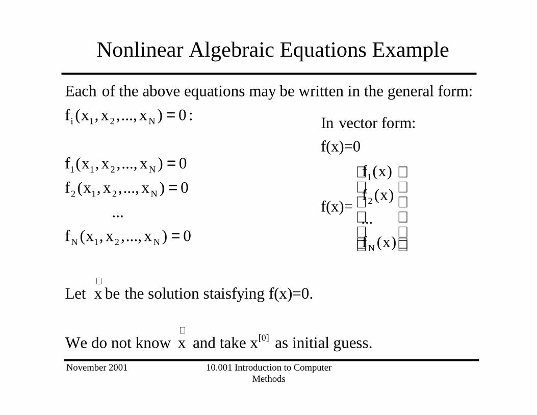
Example : f (x) (x 3)(x 2)(x 1) x 6x 11x 6
∧≈ −
≈ − = − −
−= − − − = − + −
November 2001 10.001 Introduction to ComputerMethods
Single Nonlinear Equation
November 2001 10.001 Introduction to ComputerMethods
Single Nonlinear Equation
November 2001 10.001 Introduction to ComputerMethods
Single Nonlinear Equation
For f(x)=(x-3)(x-2)(x-1)=x3-6x2+11x+6=0, we se thatNewton’s method converges to the root at x=2 only if1.6<x[0]<2.4.
We may look at the direction of the first step and seewhy: x[1]- x[0]=-f(x[0])/ f’(x[0]).
So, we have 2 “easy” roots: x=1, x=3 and a moredifficult one.
We may “factorize out” the roots we already know.

November 2001 10.001 Introduction to ComputerMethods
Single Nonlinear Equation
’’
[i+1] [i]’
f (x)Introduce g(x)
(x 3)(x 1)
f (x) f (x) 1 1g (x)
(x 3)(x 1) (x 3)(x 1) (x 3) (x 1)
We now use Newton’s method to find the roots of g(x):
g(x)x x get x 2.
g (x)
=− −
= − + − − − − − −
= − → =

November 2001 10.001 Introduction to ComputerMethods
Systems of Nonlinear Equations
Let’s extend the method to multiple equations:f1(x1,x2,x,…,xN)=0f2(x1,x2,x,…,xN)=0 => f(x)=0
….. Start from initial guess x[0]
fN(x1,x2,x,…,xN)=0
2N N Ni i
j j ki i j j kj 1 j 1 k 1j j k
[0]
As before expand each equation at the solution x with f( x )=0:
f (x) 1 f (x)f (x) f (x) (x x ) (x x ) (x x ) ...
x 2 x x
Assume x is close to x and discard quadratic terms
∧ ∧
∧ ∧∧ ∧ ∧ ∧
= = =
∧
∂ ∂= + − + − − +∂ ∂ ∂∑ ∑∑
Ni
ji jj 1 j
:
f (x)f (x) (x x )
x
∧∧
=
∂≈ −∂∑
November 2001 10.001 Introduction to ComputerMethods
Systems of Nonlinear Equations
iij
j
N
ji ij jj 1 i
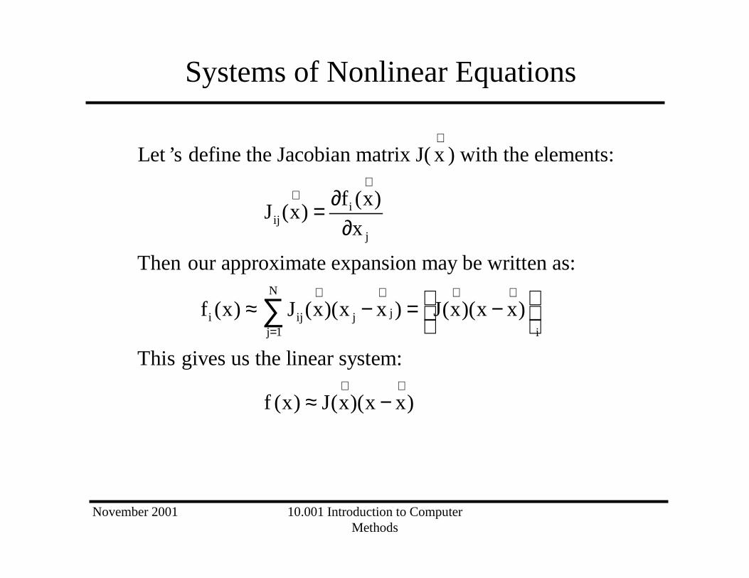
Let ’s define the Jacobian matrix J( x ) with the elements:
f (x)J (x)
x
Then our approximate expansion may be written as:
f (x) J (x)(x x ) J(x)(x x)
This gives us the linear system
∧
∧∧
∧ ∧ ∧ ∧
=
∂=∂
≈ − = − ∑:
f (x) J(x)(x x)∧ ∧
≈ −
November 2001 10.001 Introduction to ComputerMethods
Systems of Nonlinear Equations
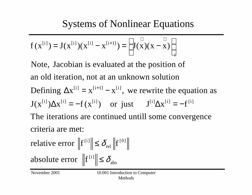
[i] [i] [i] [i 1]
i
[i] [i 1] [i]
[i]
f (x ) J(x )(x x ) J(x)(x x)
Note, Jacobian is evaluated at the position of
an old iteration, not at an unknown solution
Defining x x x , we rewrite the equation as
J(x )
∧ ∧+
+
= − = −
∆ = −∆ [i] [i] [i] [i] [i]
[i] [0]rel
[i]abs
x f (x ) or just J x f
The iterations are continued untill some convergence
criteria are met:
relative error f f
absolute error f
δ
δ
= − ∆ = −
≤
≤

November 2001 10.001 Introduction to ComputerMethods
Systems of Nonlinear Equations
Newton’s method does not always converge. If it does,can we estimate the error?
Let our function f(x) be continuously differentiable in thevicinity of x and the vector connecting x and x +p all liesinside this vicinity.
x
x+px+spT
x sp
1
0
fJ(x sp)
x
f (x p) f (x) J(x sp) pds
use path integral along the line x - x+p, parametrized by s.
+
∂+ =∂
+ = + +
−
∫

November 2001 10.001 Introduction to ComputerMethods
Systems of Nonlinear Equations
[ ]
[ ]
1
0
1
0
Add and subtract J(x)p to RHS:
f (x p) f (x) J(x) p J(x sp) J(x) p ds
In Newton’s method we ignore the integral term and
choose p to estimate f(x+p). Thus the error in this case is:
J(x sp) J(x) p ds f (x
+ = + + + −
+ − = +
∫
∫ p)
What is the upper bound on this error?
f(x) and J(x) are continuous:
J(x+sp)-J(x) 0 as p 0 for all 0 s 1.→ → ≤ ≤

November 2001 10.001 Introduction to ComputerMethods
Systems of Nonlinear Equations
[ ] [ ]
v 0
1 1
0 0
AvThe norm of the matrix is defined as: A max ,
v
Ayso for any y A , or Ay A y , therefore
y
J(x sp) J(x) pds J(x sp) J(x) ds p
The error goes down at least as fast as p because for
a continuous Jaco
≠=
≥ ≤
+ − ≤ + −∫ ∫
bian J(x+sp)-J(x) 0 as p 0.→ →
November 2001 10.001 Introduction to ComputerMethods
Systems of Nonlinear Equations
[ ] [ ]
[ ]
1 1
0 0
1
0
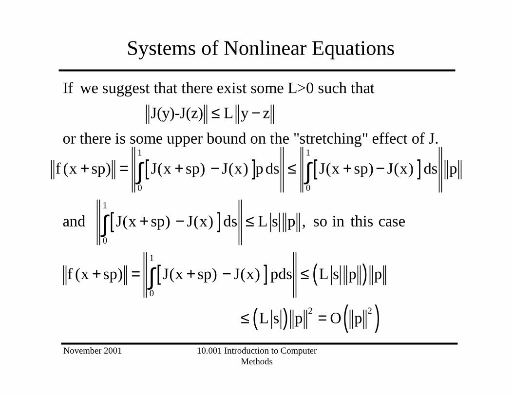
If we suggest that there exist some L>0 such that
J(y)-J(z) L y z
or there is some upper bound on the "stretching" effect of J.
f (x sp) J(x sp) J(x) pds J(x sp) J(x) ds p
and J(x sp) J(x) ds L s p , so in t
≤ −
+ = + − ≤ + −
+ − ≤
∫ ∫
∫
[ ] ( )
( ) ( )
1
0
2 2
his case
f (x sp) J(x sp) J(x) pds L s p p
L s p O p
+ = + − ≤
≤ =
∫
November 2001 10.001 Introduction to ComputerMethods
Systems of Nonlinear Equations
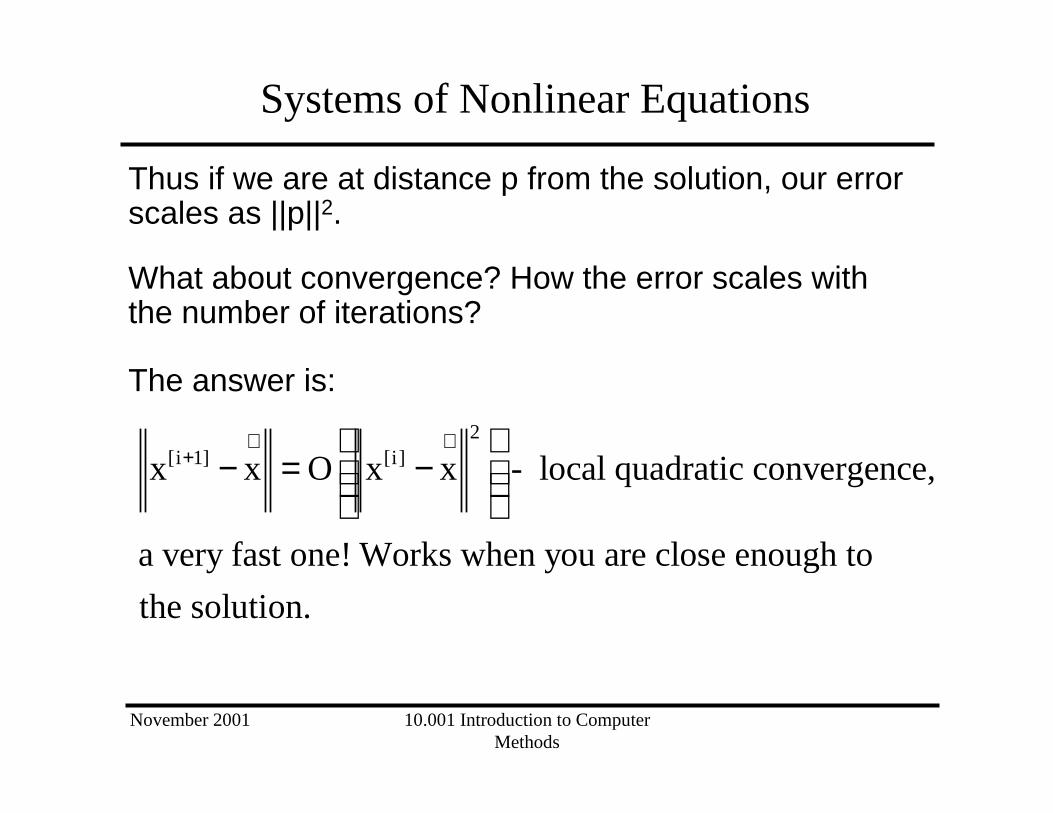
Thus if we are at distance p from the solution, our errorscales as ||p||2.
What about convergence? How the error scales withthe number of iterations?
The answer is:
2[i 1] [i]x x O x x - local quadratic convergence,
a very fast one! Works when you are close enough to
the solution.
∧ ∧+
− = −

November 2001 10.001 Introduction to ComputerMethods
Systems of Nonlinear Equations
[i] 1
[i 1] 2
[i 2] 4
[i 3] 8
x x 0.1 10
x x 0.01 10
x x 0.00001 10
x x 0.000000001 10
Works if we are close enough to an isolated
(non-singular) solution: det J( x ) 0.
∧−
∧+ −
∧+ −
∧+ −
∧
− =
− =
− =
− =
≠
�
�
�
�
November 2001 10.001 Introduction to ComputerMethods
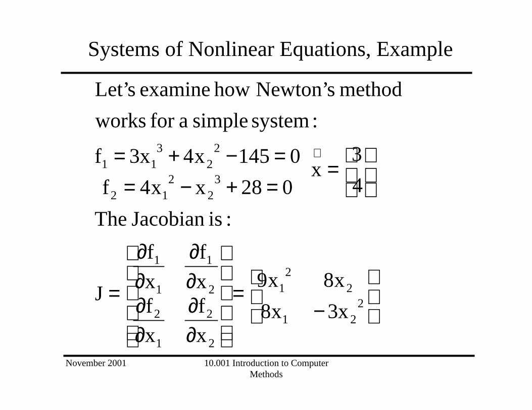
Systems of Nonlinear Equations, Example
−=
∂∂
∂∂
∂∂
∂∂
=
=
=+−==−+= ∧
221
22
1
2
2
1
2
2
1
1
1
32
212
22
311
x3x8
x8x9
x
f
x
fx
f
x
f
J
:isJacobian The
4
3x
028xx4f
0145x4x3f
:system simple afor works
method sNewton’ how examine sLet’
November 2001 10.001 Introduction to ComputerMethods
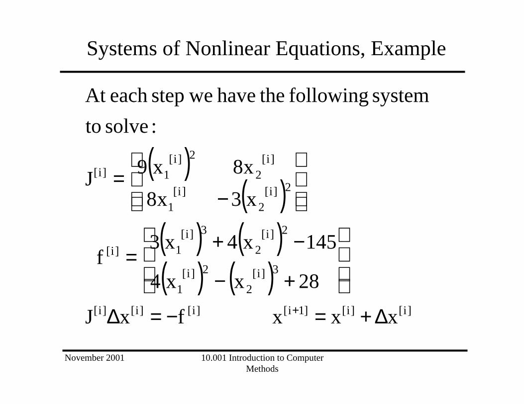
Systems of Nonlinear Equations, Example
( )( )
( ) ( )( ) ( )
]i[]i[]1i[]i[]i[]i[
3]i[2
2]i[1
2]i[2
3]i[1]i[
2]i[2
]i[1
]i[2
2]i[1]i[
xxxfxJ
28xx4
145x4x3f
x3x8
x8x9J
:solve to
system following thehave westepeach At
∆+=−=∆
+−
−+=
−=
+

November 2001 10.001 Introduction to ComputerMethods
Systems of Nonlinear Equations, Example
{ }10
bs
abs21
10
f,fmaxfcriterion
econvergenc with themethod sNewton’
of eperformanc examine usLet
−=
<=
δ
δ
November 2001 10.001 Introduction to ComputerMethods
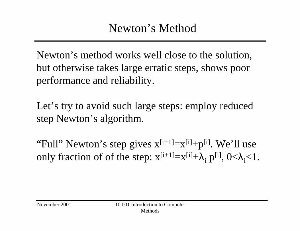
Newton’s Method
Newton’s method works well close to the solution,but otherwise takes large erratic steps, shows poorperformance and reliability.
Let’s try to avoid such large steps: employ reducedstep Newton’s algorithm.
“Full” Newton’s step gives x[i+1]=x[i]+p[i]. We’ll useonly fraction of of the step: x[i+1]=x[i]+λi p[i], 0<λi<1.

November 2001 10.001 Introduction to ComputerMethods
Newton’s Method
How do we choose λi ?Simplest way - weak line search:- start with λi =2-m for m=0,1,2,…As we reduce the value of λi bya a factor of 2 ateach step, we accept the first one that satisfies adescent criterion: ( ) ( )]i[]i[
i]i[ xfpxf <+λ
It can be proven that if the Jacobian is not singular,the correct solution will be found by the reducedstep Newton’s algorithm.


![A NONLINEAR ALGEBRAIC MULTIGRID FRAMEWORK FORbindel/papers/2018-sisc.pdf · A NONLINEAR ALGEBRAIC MULTIGRID FRAMEWORK FOR THE POWER FLOW EQUATIONS\ast ... [23, 29, 35] and Krylov](https://img.dokumen.tips/doc/110x75/5f071d047e708231d41b5f3e/a-nonlinear-algebraic-multigrid-framework-bindelpapers2018-siscpdf-a-nonlinear.jpg)