Nonlinear Acoustic Echo Cancellation for Mobile Phones: A ...lnu.diva-portal.org/smash/get/diva2:323399/FULLTEXT01.pdf · The result of this thesis has shown that it might be possible

Master’s Thesis

Anders Fhager and Jemal M. Hussien2010-06-11 Subject: Signal ProcessingLevel: AdvancedCourse code: 5ED06E

Nonlinear Acoustic Echo Cancellation for Mobile Phones: A Practical Approach

Master’s Thesis

Anders Fhager and Jemal M. Hussien

Signal Processing dvanced

5ED06E

Nonlinear Acoustic Echo Cancellation for Mobile Phones: A Practical ApproachNonlinear Acoustic Echo Cancellation for Mobile Phones: A Practical Approach

i

Abstract Acoustic echo cancelation (AEC) composes a fundamental property of speech processing to enable a pleasant telecommunication conversation. Without this property of the telephone the communicator would hear an annoying echo of his own voice along with the speech from the other communicator. This would make a conversation through any telecommunication device an unpleasant experience. AEC has been subject of interest since 1950s in the telecom industry and very efficient solutions were devised to cancel linear echo. With the advent of low cost hands free communication devices the issue of non linear echo became prominent because these devices use cheap loudspeakers that produce artifacts in addition to the desired sound which will cause non linear echo that cannot be cancelled by linear echo cancellers. In this thesis a Harmonic Distortion Residual Echo Cancelation algorithm has been chosen for further investigations (HDRES). HDRES has many of those features that are desirable for an algorithm which is dealing with nonlinear acoustic echo cancelation, such as low computational complexity and fast convergence. The algorithm was first implemented in Matlab where it was tested and modified. The final result of the modified algorithm was then implemented in C and integrated with a complete AEC system. Before the implementation a number of measurements were done to distinguish the nonlinearities that were cause by the mobile phone loudspeaker. The measurements were performed on three different mobile pones which were documented to have problems with nonlinear acoustic echo. The result of this thesis has shown that it might be possible to use an adaptive filter, which has both low complexity and fast convergence, in an operating AEC system. However, the request for such a system to work would be that a doubletalk detector is implemented along with the adaptive algorithm. That way the doubletalk situation could be found and the adaptation of the algorithm could be stopped. Thus, the major part of the speech would be saved.

ii

Acknowledgment First and foremost we would like to express our sincere gratitude to our supervisor Jonas Lundbäck at ST-Ericsson for his constant support and timely guidance throughout the thesis. His guidance in showing us ways to apply our theoretical knowledge in the practical constrained environment was priceless. We are also very grateful to Professor Sven Nordebo for his knowledgeable ideas and encouragement. We are indebted to audio department staffs of ST-Ericsson for their unreserved support and in providing a comfortable working atmosphere with a friendly approach. Finally we want to thank all who have been with us to reach at this level and gave us the opportunity to work with an interesting practical thesis in the industry.

iii

Variable notation Notation Description Dimension �� Loudspeaker input signal in time domain Vector

�� Microphone input signal in time domain Scalar

�� Loudspeaker input signal in frequency domain Vector

�� Microphone input signal in frequency domain Scalar

�� Adaptive linear filter Vector

�� Linear kernel of Volterra filter Vector

�� Quadratic kernel of Volterra filter Vector

�� Estimated acoustic echo in time domain Scalar

� �� Estimated acoustic echo in frequency domain Scalar

�� Output of linear filter Scalar

�� Output of Volterra filter Scalar

�� Error from Volterra filter Scalar

�� Error from linear filter Scalar

�� Error from combined filter (overall error) Scalar

�� Step size of linear kernel in Volterra filter Scalar

�� Step size of quadratic kernel in Volterra filter Scalar

�� Step size of linear filter Scalar

�� Weighting parameter Scalar

�� Output signal of HDRES in time domain Scalar

�� Output signal of HDRES in frequency domain Scalar

�� Nonlinear modelling Vector

�� Basis functions Vector

�� Matrix of the bias function Matrix

�� Signal after non linear model Vector

�� Non linear coefficient Vector

�� Output of shortening filter Scalar

�� Estimated shortening filter output Scalar

�� Shortening filter Vector

�! �" Transpose operation �! �# Hermitian transpose operation

iv

Symbol explanations

Loudspeaker

Microphone

Multiplication of two or more signals

Addition of two or more signals

Subtraction of two signals

Adaptive filter

Update of an Adaptive filter

v

List of figures Figure 1.1 Acoustic Echo in hands free communication .................................................................................... 3 Figure 1.2 Block diagram of acoustic echo canceller ......................................................................................... 4 Figure 1.3 Adaptive filter in acoustic echo canceller ......................................................................................... 5 Figure 1.4 Simplified figure of the function of a loudspeaker ......................................................................... 12 Figure 1.5 Sinusoidals with different frequencies. From above: 25, 50 and 75 Hz respectively ..................... 13 Figure 1.6 Summation of the three sinusoidals ............................................................................................... 14 Figure 1.7 The corresponding signal of figure 1.6 in frequency domain ......................................................... 14 Figure 1.8 Block diagram of acoustic echo control .......................................................................................... 16 Figure 2.1 An illustration of the measurement setup...................................................................................... 18 Figure 2.2 Capturing measurement data ......................................................................................................... 18 Figure 2.3 Hands free mode............................................................................................................................. 19 Figure 2.4 External microphone ....................................................................................................................... 19 Figure 2.5 Frequency sweep with decreasing amplitude, time domain plot .................................................. 20 Figure 2.6 Pulses of white cyclo stationary noise, time domain...................................................................... 20 Figure 2.7 Loudspeaker input. Frequency sweep with a high amplitude, frequency domain ........................ 21 Figure 2.8 Microphone input. Frequency sweep with a high amplitude, frequency domain ......................... 21 Figure 2.9 Loudspeaker input. Frequency sweep with a low amplitude, frequency domain. ........................ 21 Figure 2.10 Microphone input. Frequency sweep with a low amplitude, frequency domain. ....................... 21 Figure 2.11 Loudspeaker input. Frequency sweep with a high amplitude, frequency domain ...................... 22 Figure 2.12 Microphone input. Frequency sweep with a high amplitude, frequency domain ....................... 22 Figure 2.13 Microphone input. Frequency sweep with a low amplitude, frequency domain ........................ 22 Figure 2.14 Loudspeaker input. Frequency sweep with a low amplitude, frequency domain ....................... 22 Figure 2.15 Loudspeaker input. White noise, frequency domain ................................................................... 22 Figure 2.16 Microphone input. White noise, frequency domain .................................................................... 22 Figure 3.1 Combination of filters scheme ........................................................................................................ 31 Figure 3.2 Simplified combination of kernels scheme ..................................................................................... 32 Figure 3.3 Nonlinear AEC – Hammerstein model (adaptive) ........................................................................... 34 Figure 3.4 AEC nonlinear Hammerstein design together with a shortening filter .......................................... 35 Figure 3.5 A illustration of the architecture of a shortening filter .................................................................. 35 Figure 3.6 A simplified illustration of how the HDRES and the linear AEC works together............................. 39 Figure 3.7 Illustrates the architecture of the HDRES model together with a linear AEC ................................. 40 Figure 4.1 Flowchart of the HDRES model ....................................................................................................... 45 Figure 4.2 Table of the mapping matrix for the first overtone ........................................................................ 48 Figure 4.3 Table of the mapping matrix for the first overtone ........................................................................ 49 Figure 4.4 The input signal created for testing of the HDRES algorithm in Matlab ......................................... 50 Figure 4.5 Plot of the true residual echo ......................................................................................................... 51 Figure 4.6 Plot of the estimate of the true residual echo ................................................................................ 51 Figure 4.7 The error function, gives the difference between the true residual echo and its estimation ....... 52 Figure 4.8 Block diagram of acoustic echo canceller ....................................................................................... 55 Figure 5.1 Illustration of the loudspeaker input signal. .................................................................................. 59 Figure 5.2 Illustration of the microphone input signal .................................................................................... 59 Figure 5.3 Illustration of the output of the linear AEC .................................................................................... 59 Figure 5.4 Illustration of the output of the HDRES algorithm ......................................................................... 60 Figure 5.5 Illustration of the output of the static method output ................................................................... 60 Figure 5.6 Illustration of the output of the linear AEC magnified ................................................................... 60 Figure 5.7 Illustration of the output of the HDRES output magnified ............................................................. 61 Figure 5.8 Illustration of the output of the static output magnified ............................................................... 61 Figure 5.9 Illustration of the loudspeaker input signal. It contains speech with different amplitudes........... 61 Figure 5.10 Illustration of the microphone input signal .................................................................................. 62 Figure 5.11 Illustration of the output of the linear AEC .................................................................................. 62 Figure 5.12 Illustration of the output of HDRES .............................................................................................. 62 Figure 5.13 Illustration of the static output ..................................................................................................... 62 Figure 5.14 Illustration of the HDRES output magnified ................................................................................. 63 Figure 5.15 Illustration of the static output magnified .................................................................................... 63

vi

Figure 5.16 Illustration of the output of the linear AEC .................................................................................. 64 Figure 5.17 Illustration of the output of the HDRES ........................................................................................ 64 Figure 5.18 Illustration of the output of the static method ............................................................................ 64 Figure 5.19 NERLE of HDRES algorithm in Hands free mode (single talk) ....................................................... 65 Figure 5.20 NERLE of Static method in hands free mode (single talk) ............................................................ 66 Figure 5.21 NERLE of HDRES algorithm in hand held mode (single talk) ......................................................... 66 Figure 5.22 NERLE of the static method in hand held mode (single talk) ....................................................... 67

vii

List of tables Table 3.1 Frequency bands for narrow band speech with their frequency range .......................................... 26 Table 3.2 The result of calculating harmoincs for the 6th band ...................................................................... 27 Table 3.3 Complete mapping table .................................................................................................................. 28 Table 4.1 Extract of the Matlab code for the calculation of the frequency band ........................................... 46 Table 4.2 Extract of the Matlab code for the call of the mapping matrix ....................................................... 46 Table 4.3 Extract of the Matlab code for the calculation of the estimation ................................................... 46 Table 4.4 Extract of the Matlab code for the averaging calculation................................................................ 47 Table 4.5 Limiting the weights ......................................................................................................................... 47 Table 4.6 A part of the Matlab code that calculated the MappingMatrix ....................................................... 47 Table 4.7 Residual echo estimation ................................................................................................................. 54 Table 4.8 Updating of the weights .................................................................................................................. 55 Table 4.9 Double to SPL type conversion ........................................................................................................ 56

viii

Table of contents Abstract ............................................................................................................................................................... i

Acknowledgment ............................................................................................................................................... ii

Variable notation .............................................................................................................................................. iii

Symbol explanations ......................................................................................................................................... iv

List of figures ...................................................................................................................................................... v

List of tables ......................................................................................................................................................vii

CHAPTER 1 INTRODUCTION ............................................................................................................................... 1

1.1 Report organisation ................................................................................................................................. 2

1.2 Acoustic echo cancellation ...................................................................................................................... 3

1.2.1 Types of echo .................................................................................................................................... 3

1.2.2 Echo cancellation .............................................................................................................................. 4

1.2.3 LEM System ....................................................................................................................................... 4

1.2.4 Adaptive Filter ................................................................................................................................... 4

1.2.5 Non linear Processor (NLP) ............................................................................................................... 4

1.3 Adaptive filter algorithms ........................................................................................................................ 5

1.3.1 The Steepest Descent method .......................................................................................................... 6

1.3.2 Least Mean Square (LMS) algorithm ................................................................................................. 7

1.3.3 Normalized LMS (NLMS) Algorithm .................................................................................................. 8

1.3.4 Recursive Least Squares (RLS) algorithm .......................................................................................... 9

1.4 Loudspeaker nonlinear distortion .......................................................................................................... 12

1.4.1 Loudspeaker description ................................................................................................................. 12

1.4.2 Nonlinear distortion ........................................................................................................................ 12

1.4.3 Origin of the nonlinearities ............................................................................................................. 13

1.4.4 Harmonics ....................................................................................................................................... 13

1.5 Modelling physical systems ................................................................................................................... 15

1.5.1 Data collection ................................................................................................................................ 15

1.5.2 Selecting model structure ............................................................................................................... 15

1.5.3 Parameter estimation ..................................................................................................................... 15

1.5.4 Model validation ............................................................................................................................. 15

1.6 Description of Acoustic Echo Control Implementation ......................................................................... 16

1.6.1 Overview of Acoustic Echo Control Implementation...................................................................... 16

CHAPTER 2 MEASUREMENTS ........................................................................................................................... 17

2.1 Measurement procedure ....................................................................................................................... 18

2.1.1 Measurement type 1: Hand held mode .......................................................................................... 19

2.1.2 Measurement type 2: Hands free mode ......................................................................................... 19

2.1.3 Measurement type 3: Measurement with an external microphone. ............................................. 19

2.2 Measurement analysis ........................................................................................................................... 20

2.2.1 Input signals .................................................................................................................................... 20

ix

2.2.2 Hand held mode .............................................................................................................................. 21

2.2.3 Hands free mode............................................................................................................................. 22

2.2.4 Measurement with an external microphone. ................................................................................. 23

2.3 Measurement result .............................................................................................................................. 23

CHAPTER 3 POSSIBLE SOLUTIONS .................................................................................................................... 24

3.1 Static method ......................................................................................................................................... 25

3.1.1 Nonlinear loudspeaker effects ........................................................................................................ 25

3.1.2 Harmonic distortion ........................................................................................................................ 25

3.1.3 Harmonic Activation Level .............................................................................................................. 25

3.1.4 Harmonic Gains ............................................................................................................................... 25

3.1.5 Fundamental Gains ......................................................................................................................... 26

3.1.6 Mapping table ................................................................................................................................. 26

3.1.7 Harmonic distortion estimation ...................................................................................................... 26

3.1.8 Mapping table construction ............................................................................................................ 26

3.1.9 Summary ......................................................................................................................................... 28

3.2 Volterra filters ........................................................................................................................................ 29

3.2.1 Introduction .................................................................................................................................... 29

3.2.2 Mathematical description ............................................................................................................... 29

3.2.3 Adaptation of Volterra filters .......................................................................................................... 29

3.2.4 Application of Volterra filter for Acoustic Echo Cancellation ......................................................... 30

3.2.5 Combination of Filters Scheme (CFS) .............................................................................................. 30

3.2.6 Description of the combination ...................................................................................................... 31

3.2.7 Combination of Kernels Scheme(CKS) ........................................................................................... 32

3.2.8 Limitation of volterra filter ............................................................................................................. 33

3.3 Hammerstein model .............................................................................................................................. 34

3.3.1 Introduction .................................................................................................................................... 34

3.3.2 AEC nonlinear Hammerstein design together with a shortening filter .......................................... 35

3.3.3 Mathematical representation ......................................................................................................... 36

3.4 Harmonic distortion residual echo suppressor (HDRES) ....................................................................... 39

3.4.1 Introduction .................................................................................................................................... 39

3.4.2 Residual echo suppression (RES) .................................................................................................... 39

3.4.3 System architecture ........................................................................................................................ 39

3.4.4 Modulated Complex Lapped Transform (MCLT) ............................................................................. 40

3.4.5 Mathematical representation ......................................................................................................... 40

CHAPTER 4 IMPLEMENTATION ........................................................................................................................ 43

4.1 Implementation in Matlab ..................................................................................................................... 44

4.1.1 Summary of the four methods........................................................................................................ 44

4.1.2 Changes from the article ................................................................................................................. 44

4.1.3 Additional changes from development .......................................................................................... 45

4.1.4 Frequency banding ......................................................................................................................... 45

x

4.1.5 Call for the mapping matrix ............................................................................................................ 46

4.1.6 Estimation ....................................................................................................................................... 46

4.1.7 Averaging ........................................................................................................................................ 47

4.1.8 Limiting the weights ........................................................................................................................ 47

4.1.9 The MappingMatrix function .......................................................................................................... 47

4.1.10 Mathematical explanation ............................................................................................................ 48

4.1.11 Matlab results ............................................................................................................................... 50

4.2 C- Implementation ................................................................................................................................. 53

4.2.1 Signal Processing Library (SPL) ........................................................................................................ 53

4.2.2 Inputs to HDRES algorithm in C ....................................................................................................... 53

4.2.3 HDRES algorithm in C ...................................................................................................................... 54

4.2.4 Location of HDRES ........................................................................................................................... 55

CHAPTER 5 RESULTS ......................................................................................................................................... 57

5.1 Introduction ........................................................................................................................................... 58

5.2 Results for echo subtraction .................................................................................................................. 58

5.2.1 Hand held mode .............................................................................................................................. 59

5.2.2 Hands free mode case .................................................................................................................... 61

5.2.3 Results for the double talk situation ............................................................................................... 63

CHAPTER 6 CONCLUSION AND FURTHER WORK ............................................................................................. 68

6.1 Conclusion .............................................................................................................................................. 69

6.2 Further work .......................................................................................................................................... 70

References ....................................................................................................................................................... 71

Appendix A Matlab Code ................................................................................................................................. 73

Appendix B Measurement plots ...................................................................................................................... 77

Appendix C Result plots ................................................................................................................................... 91

1

CHAPTER 1 INTRODUCTION

2

1.1 Report organisation The thesis report has the following content:

In chapter 1 introduction to the subject matter where the concept of acoustic echo cancelling and loudspeaker nonlinearities are explained. In chapter 2 a description of the performed measurements is done. It includes among others the measurement setup and the discoveries that were made. Chapter 3 gives a deeper description of the different methods to cancel nonlinear acoustic echo that were chosen for further investigation. In chapter 4 the implementation of the choosen algorithm in Matlab and in C is presented. It includes descriptions of important sections of the algorithm, implementation difficulties and testing results. In chapter 5 results of the thesis are presented. The results are shown by plots and explanation of the plots according to the expected theoretical result. In chapter 6 the conclusion and the further work is stated.

3

1.2 Acoustic echo cancellation Webster dictionary defines echo as: “A wave that has been reflected or otherwise returned with sufficient magnitude and delay to be detected as a wave distinct from that directly transmitted.” Echo in a telecommunication system degrades the quality and intelligibility of voice communication. Although echo is used in detection and navigation applications such as radar and infrared imaging as a useful phenomenon, it’s undesirable in communications systems. Hence efforts are done to reduce it as much as possible. The effect of echo on voice communication is dependent on amplitude and time delay. A delay above 20ms is considered as annoying while more than 200ms is disruptive [3].

1.2.1 Types of echo There are two types of echo in Telecommunication

1. Hybrid Echo

Hybrid echo is an electrical echo generated by public-switched telephone network (PSTN) due to impedance mismatch between the two wire subscriber line and four wire long distance telephone lines.

2. Acoustic echo Acoustic echo is observed when sound from a loudspeaker is picked up by microphone in the same device and sent back to the original source of the sound with significant delay. If the delay is small, then the acoustic echo is perceived as soft reverberation. But if the delay is too large it will be annoying and disruptive hence should be cancelled. Acoustic echo is mostly experienced in hands free communications as shown in figure 1.1 [1].

Figure 1.1 Acoustic Echo in hands free communication

Far-end Near-end

Direct path

Reflected path

4

1.2.2 Echo cancellation The endeavor to cancel echo started in the late 1950s. Primitive echo suppressors use voice activated switches to turn off the receiving line allowing voice to pass on the transmitting line only. They effectively block echo, but have a problem of allowing only half-duplex communication where only one end is allowed to talk at a time. Line echo cancellers were constructed to remove electrical echo from telephone lines and are very efficient [11]. However the problem of acoustic echo cancellation is a more challenging task since the acoustic path is not known at priori. Moreover it changes constantly. That’s why development of adaptive methods was crucial for this task. Acoustic echo cancellers (AEC) try to cancel echo by adaptively modeling the loudspeaker-enclosure-microphone (LEM) system and hence estimating the acoustic echo by using loudspeaker input signal coming from far end to be subtracted from the microphone input signal. Figure 1.2 shows block diagram of simplified acoustic echo canceller which consists of three components [14].

Figure 1.2 Block diagram of acoustic echo canceller

1.2.3 LEM System The loudspeaker-enclosure-microphone system includes a loudspeaker, a microphone and the direct and reflected acoustic echo paths of the echo. The performance of the AEC depends on how well the adaptive filter modelled the LEM system, which directly dictates how close the estimated echo is to the real microphone input echo [14].

1.2.4 Adaptive Filter This is the crucial component of the acoustic echo canceller that estimates echo adaptively by keeping track of the changes in room acoustics. For a very good LEM system which does not introduce nonlinear artifacts to the loudspeaker input signal the echo can be considered as a delayed and attenuated version of the loudspeaker input signal. In such cases a linear AEC can accurately estimate the echo by using linear adaptive filters. Generally the LEM is modelled as a linear system which explains why linear adaptive filters are usually used at this position of the acoustic echo canceller. An explanation of the most commonly used linear adaptive algorithms, LMS and RLS, is given in section 1.3 [14].

1.2.5 Non linear Processor (NLP) NLP in AEC is the block which handles non linear processing that cannot be done by the linear adaptive filter. Studies have shown that loudspeakers produce nonlinear artifacts. Consequently linear adaptive filters cannot estimate these nonlinearities and hence such echo will not be cancelled if only the usual linear adaptive filters are used. Residual echo control in NLP tries to suppress residual echo by modeling the non linearity in LEM system. The NLP then generates comfort noise if output power of residual echo control is lower than background noise level. Otherwise the far end may think the communication link is disconnected. Introduction to modeling of physical systems is given in section 1.5[14].

5

1.3 Adaptive filter algorithms For any type of adaptive filter applications the choice of adaptive algorithm plays an important role for the performance of the overall system. Two widely used adaptive algorithms are LMS and RLS. Both algorithms try to minimize the mean square error. The choice of algorithm depends on rate of convergence, amount of error at convergence, robustness of the algorithm in initial states, computational complexity and memory usage [3]. Before explaining the LMS and RLS algorithm, a description of the steepest descent algorithm is given since it is the base for derivation of LMS. Figure 1.3 shows the overall system with input, output and intermediate signals which will be used in subsequent sections.

Figure 1.3 Adaptive filter in acoustic echo canceller

The error and the estimated desired signals are defined as: �� $ �� % ��& (1.1)

�� $ &�'��& (1.2)

Substituting equation (1.2) in equation (1.1) �� $ �� % �'�� (1.3) The mean square error:

()��* $ ()+�� % �'��,�* (1.4) ()��* $ ()+��,� % -�'�� . +�'��,�* (1.5) ()��* $ ()+��,�* % -�'�� . �'��()��'��*��& (1.6)

Computing the mean for each term in equation (1.6) results in: ()��* $ /00 % -�'��/10 .&�'��/11�� (1.7)

6

where, /00&23&4567�788�94627�&:4682�&7;&6��&��328��&32<�49 /01 &23&�8733&�788�94627�&7;&6��&8�;�8��&4��&��328��&32<�49 /00&23&4567�788�94627�&:4682�&7;&6��&8�;�8��&32<�49

1.3.1 The Steepest Descent method The Steepest Descent method is a method used to find the optimum solution (minimum point) of a function by taking small steps in the negative gradient direction [3]. In adaptive filtering applications the error, the difference between the estimated and desired signals, is expressed as a function of filter coefficients. Applying this method to the mean square error function results in optimum filter coefficients of the adaptive filter. Starting with initial filter coefficients, the method continuously updates the coefficients in a downward direction until a minimum point, where the gradient is zero, is reached. The steepest descent method adaptation: �� . =� $ �� . &��%>()��*� (1.8)

where, ()��*&23&6��&:�4�&3�548�&�8878 >()��&23&<84�2��6&7;&6��&:�4�&3�548�&�8878 �&23&6��&4�4�64627�&36��&32 �

From equation (1.7) one has the expression for the mean square error. Computing its gradient gives: >()��* $ &%-/10 . &-/11�� (1.9)

The optimum filter coefficient (�?) is found when the gradient is zero. Equating equation (1.9) to zero and solving for h gives:

�? $ &/11@/10& (1.10)

Substituting equation (1.9) in equation (1.8) �� . =� $ �� . &��/10 % /11��&� (1.11) Let us define filter coefficient error �A as:

�A�� $ �� %&�? (1.12)

Subtracting �? from both sides of equation (1.12) and then substituting /11�? for /10 finally using equation (1.12) yields:

�A�� . =� $ �A�� % &-�/11�A�� (1.13)

The correlation matrix /11 can be expressed in terms of eigen vectors and eigen values as follows: /11 $ �B�' (1.14)

where, � is orthonormal matrix of eigen vectors of /11 B is diagonal matrix with eigen values of /11 as diagonal elements

7

Substituting equation (1.14) in equation (1.13):

�A�� . =� $ �A�� % &-��B�'�A�� (1.15)

Multiply both sides of equation (1.15) by �'

�'&�A�� . =� $ &�'�A�� % &-��B+�',��A�� (1.16)

Let

C�� $ �'�A�� (1.17)

Hence equation (1.16) becomes C�� . =� $ &C�� % -�BC�� (1.18)

Since B is a diagonal matrix, equation (1.19) can be expressed in terms of individual eigen vectors CD�� . =� $ &CD�� % -�EFCD�� (1.19)

The solution for the recursion in equation (1.19) can be written as CD�� . =� $ �= % -�EF�DCD�� (1.20)

The convergence of equation (1.20) is guaranteed if the following condition is fulfilled G= % -�EFG H =, for all k (1.21)

Or equivalently, if

� H & IJ , for all k (1.22)

The convergence criterion of equation (1.22) is summarized as

� H &

IKLM&& (1.23)

where ENOP is the largest eigen value

For ease of implementation the convergence criteria is given as:

� H &QROST�UVV� &W &

IKLM&& (1.24)

1.3.2 Least Mean Square (LMS) algorithm LMS is a simple yet effective adaptive algorithm that is used in echo cancellation, channel equalization, adaptive noise cancellation, and time-delay estimation. LMS simplifies the Steepest Descent method by computing the gradient of instantaneous squared error function instead of the average squared error [3]. Step size determines the rate of convergence and amount of Mean Square Error (MSE) at convergence. A large step size will result in a fast rate of convergence but with high MSE, while a small step size results in a slow rate of convergence with minimum MSE. The Steepest Descent adaptation in equation (1.8) with instantaneous squared error is:

8

�� . =� $ �� . &��%>�� (1.25) where, �� $ �� % �'�� (1.26)

Computation of the gradient is: >�� $ %-��+�� % �'��, (1.27)

Substituting the error in equation (1.27) >�� $ %-�� (1.28)

Inserting equation (1.27) in equation (1.25) gives the adaptation for LMS algorithm: �� . =� $ �� . &-�� (1.29)

Incorporating the constant in the step size �, the adaptation becomes �� . =� $ �� . &�� (1.30)

Summary of LMS algorithm

Given initial parameter&�X,

Repeat for � $ =Y-YZY[

�� $ �� % �'�� (1.31)

�� . =� $ �� . &�� (1.32)

1.3.3 Normalized LMS (NLMS) Algorithm NLMS is a variant of the LMS algorithm that normalizes the adaptation step size according to the power of the input signal, so that the convergence of the LMS algorithm will not slow down by small signals and increase by large signals [4]. Consider the convergence criteria of the Steepest Descent method in equation (1.25). It relies on the autocorrelation matrix to set the step size. Practically the autocorrelation matrix is unknown. Therefore its approximate is calculated as: 684��/11� $ �\ .=�()G��G�* (1.33)

where, \ is the size of /11 ()G��G�} is power of input signal

Power of the input signal can be estimated as:

()G��G�* &] & \^ &_ G�� % `�G�\DaX (1.34)

Substituting equation (1.31) in equation (1.30), the convergence criteria becomes

� H &bcdef�UVV� $&

&_ G1�g@D�Gh\ijk $& &1l�g�1�g�& (1.35)

9

Computing step-size in time one has:

� $ & mG1�g�Gh& (1.36)

where n is normalized step size in the range 0 <&n <2

To avoid division by zero in equation (1.36) a very small number (machine precision number) is added in the denominator:

� $ & mG1�g�Gh^&d (1.37)

The adaptation algorithm for NLMS is found by substituting equation (1.37) in equation (1.29)

�� . =� $ �� .&& mG1�g�Gh^d �� (1.38)

where 4 is a small positive number and n is the step size.

1.3.4 Recursive Least Squares (RLS) algorithm RLS is an adaptive algorithm which tries to minimize the Mean Square Error (MSE). It is a time update version of the well-known wiener filter. It has fast convergence rate to the optimal solution, high performance for non-stationary signals and low minimum MSE at convergence. These attributes makes it suitable for speech enhancement, channel equalization, and echo cancellation applications [3][5]. The least square cost function as ;g�� is given by ;g�� $ &_ �g@DgDa G�o��`� % ��`�G� .&�� % �X�o�g/X�� % �X� (1.39)

where /X&4��&�X&&are initial values Define ;?�� $ �� % �X�o/X�� % �X�&& (1.40)

�g�� $ /X�X (1.41)

Introduce A and b as:

p $ q�rsth &�o�=�Y u Y �o��v', � $ q�rst

h &�w�=�Y u Y �w��v'

Hence, the cost function in equation (1.39) can be written as: ;g�� $ �p� % ��o�p� % �� . �� % �?�o�g/X�� % �X�& (1.42) The “forgetting factor”, �, determines where the emphasis will be depending on how large � is. The forgetting factor is neglected when � $ =! The solution for the cost function is found by differentiating equation (1.42) with respect to �: �g $ /g@�g (1.43)

/g $ pop .&�g/X $&_ �g@D��`��o�`� . �g/XgDa & (1.44) �g $ po� .&�g�X $ _ �g@D��`��w�`� . �g�XgDa (1.45)

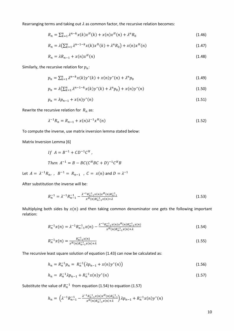
10

Rearranging terms and taking out � as common factor, the recursive relation becomes: /g $ _ �g@D��`��o�`� . ��o�� . �g/XgDa (1.46)

/g $ �x_ �g@@D��`��o�`� . �g/XgDa y . ��o�� (1.47) /g $ �/g@ . ��o�� (1.48)

Similarly, the recursive relation for �g: �g $ _ �g@D��`��w�`� . ��w�� . �g�XgDa (1.49)

�g $ �x_ �g@@D��`��w�`� . �g�XgDa y . ��w�� (1.50) �g $ ��g@ . ��w�� (1.51)

Rewrite the recursive relation for /g as: �@/g $ /g@ . ��@�o�� (1.52)

To compute the inverse, use matrix inversion lemma stated below: Matrix Inversion Lemma [6] z;&&p $ {@ . |}@|o&Y

~��&&p@ $ { % {|�|o{| . }�@|o{

Let p $&�@/g, , &{@ $&/g@ , | $ &�� and } $ �@ After substitution the inverse will be:

/g@ $ �@/g@@ % �stUrstst 1�g�1l�g�Urstst1l�g�Urstst 1�g�^� (1.53)

Multiplying both sides by �� and then taking common denominator one gets the following important relation:

/g@�� $ �@/g@@ �� % �stUrstst 1�g�1l�g�Urstst 1�g�1l�g�Urstst 1�g�^� (1.54)

/g@�� $ Urstst 1�g�1l�g�Urstst 1�g�^� (1.55)

The recursive least square solution of equation (1.43) can now be calculated as:

�g $ /g@�g $&/g@x��g@ . ��w��y (1.56) �g $&/g@��g@ . /g@��w�� (1.57)

Substitute the value of /g@& from equation (1.54) to equation (1.57)

�g $&��@/g@@ % �stUrstst 1�g�1l�g�Urstst1l�g�Urstst 1�g�^� � ��g@ . /g@��w��

11

&&&&$ &/g@@ �g@ %&�@/g@@ ��o��/g@@ ��g@�o��/g@@ �� . � . /g@��w�� &&&$ &�g@%&/g@��o��g@ . /g@��w�� &&&$ &�g@.&/g@��w�� % �o��g@� �� &$ &�g@.&/g@��w�� (1.58)

where, �� $ �� % �g@o �� (1.59) Summary of RLS algorithm:

Given initial parameters, �XY /XY /X@

Repeat for � $ =Y-YZY[

�� $ �� % �g@o �� (1.60)

/g@ $ �@/g@@ % �stUrstst 1�g�1l�g�Urstst1l�g�Urstst 1�g�^� (1.61)

�� &$ &�g@.&/g@��w�� (1.62)

12

1.4 Loudspeaker nonlinear distortion

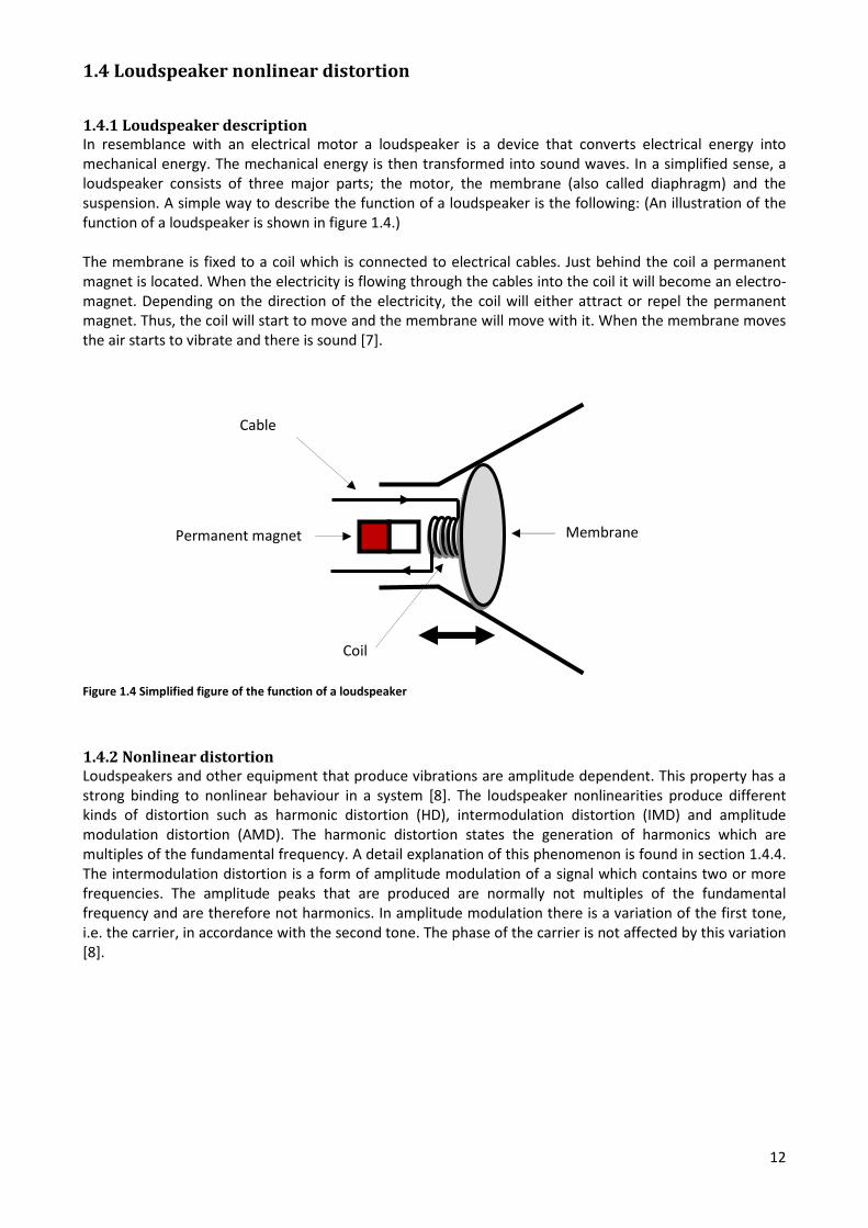
1.4.1 Loudspeaker description In resemblance with an electrical motor a loudspeaker is a device that converts electrical energy into mechanical energy. The mechanical energy is then transformed into sound waves. In a simplified sense, a loudspeaker consists of three major parts; the motor, the membrane (also called diaphragm) and the suspension. A simple way to describe the function of a loudspeaker is the following: (An illustration of the function of a loudspeaker is shown in figure 1.4.) The membrane is fixed to a coil which is connected to electrical cables. Just behind the coil a permanent magnet is located. When the electricity is flowing through the cables into the coil it will become an electro-magnet. Depending on the direction of the electricity, the coil will either attract or repel the permanent magnet. Thus, the coil will start to move and the membrane will move with it. When the membrane moves the air starts to vibrate and there is sound [7]. Figure 1.4 Simplified figure of the function of a loudspeaker

1.4.2 Nonlinear distortion Loudspeakers and other equipment that produce vibrations are amplitude dependent. This property has a strong binding to nonlinear behaviour in a system [8]. The loudspeaker nonlinearities produce different kinds of distortion such as harmonic distortion (HD), intermodulation distortion (IMD) and amplitude modulation distortion (AMD). The harmonic distortion states the generation of harmonics which are multiples of the fundamental frequency. A detail explanation of this phenomenon is found in section 1.4.4. The intermodulation distortion is a form of amplitude modulation of a signal which contains two or more frequencies. The amplitude peaks that are produced are normally not multiples of the fundamental frequency and are therefore not harmonics. In amplitude modulation there is a variation of the first tone, i.e. the carrier, in accordance with the second tone. The phase of the carrier is not affected by this variation [8].

Coil

Cable

Membrane Permanent magnet

13

1.4.3 Origin of the nonlinearities

1.4.3.1 Suspension The suspension system in a loudspeaker is used to make the coil fall back to its orginal position after its movement. At low amplitudes there is a linear relationship between the back-falling force and the displacement widthways but for higher amplitudes this is not the case. These properties will cause nonlinear stiffness which generates harmonic distortion [8].

1.4.3.2 The force factor The force factor describes the relation between the electricity in the coil and the force that attracts or repels the permanent magnet. The force factor depends on the position of the coil and the magnetic field generated by the permanent magnet. The asymmetry of the force factor and the voice coil displacement causes the nonlinearity which generates harmonic distortion, intermodulation distortion and amplitude distortion [8].

1.4.4 Harmonics The frequency of a harmonic is a multiple of the fundamental frequency of the original wave. The first multiple, fundamental frequency times one is defined to be the first harmonic. Thus, the first harmonic is equivalent with the fundamental frequency. The second multiple of the fundamental frequency is the second harmonic and so forth. For a deeper understanding consider the following example [10]. Three sinusoidals which have the frequencies 25, 50 and 75 Hz are represented in figure 1.5. These three signals are summed in&�b?b into one signal. The sinusoidal with the lowest frequency of all the sinusoidals, in this case&�, is the first harmonic. ��, which has twice the frequency of&�, is called the second harmonic. �� is called the third harmonic because it has three times the frequency of&�. The summation,&�b?b, of these three sinusoidals is shown in figure 1.6 and the corresponding signal in frequency domain in figure 1.7 [10].

Figure 1.5 Sinusoidals with different frequencies. From above: 25, 50 and 75 Hz respectively

�Q�Q $&� . �� .&��

� $ ��-π& w -�&�� $ ��-π& w ��&�� $ ��-π& w ��&��

14

In frequency domain it is easy to see that the fundamental frequency is the first peak at 25 Hz and that the two harmonics appear at 50 and 75 Hz respectively.

1.4.4.1 Harmonic distortion The harmonic distortion is a measure of the effect of harmonics in an audio signal. It describes the amplitude relation between the fundamental frequency and the harmonics and it is given as a percentage. The calculation of total harmonic distortion is given by:

~�} $&�� .�� .u.�g�� &�&=��

where � is the first harmonic, ��&is the second and so forth.

Figure 1.7 The corresponding signal of figure 1.6 in frequency domain

Figure 1.6 Summation of the three sinusoidals

15

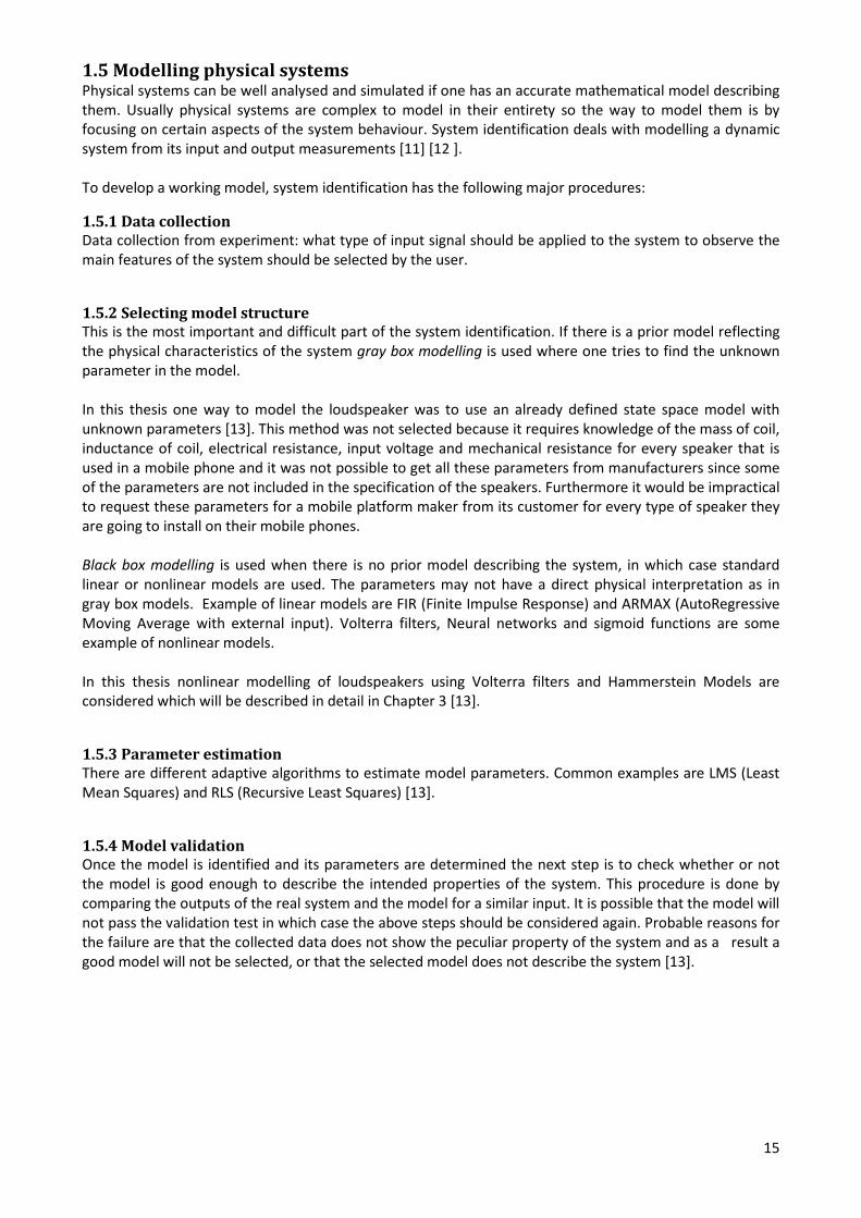
1.5 Modelling physical systems Physical systems can be well analysed and simulated if one has an accurate mathematical model describing them. Usually physical systems are complex to model in their entirety so the way to model them is by focusing on certain aspects of the system behaviour. System identification deals with modelling a dynamic system from its input and output measurements [11] [12 ]. To develop a working model, system identification has the following major procedures:

1.5.1 Data collection Data collection from experiment: what type of input signal should be applied to the system to observe the main features of the system should be selected by the user.

1.5.2 Selecting model structure This is the most important and difficult part of the system identification. If there is a prior model reflecting the physical characteristics of the system gray box modelling is used where one tries to find the unknown parameter in the model. In this thesis one way to model the loudspeaker was to use an already defined state space model with unknown parameters [13]. This method was not selected because it requires knowledge of the mass of coil, inductance of coil, electrical resistance, input voltage and mechanical resistance for every speaker that is used in a mobile phone and it was not possible to get all these parameters from manufacturers since some of the parameters are not included in the specification of the speakers. Furthermore it would be impractical to request these parameters for a mobile platform maker from its customer for every type of speaker they are going to install on their mobile phones. Black box modelling is used when there is no prior model describing the system, in which case standard linear or nonlinear models are used. The parameters may not have a direct physical interpretation as in gray box models. Example of linear models are FIR (Finite Impulse Response) and ARMAX (AutoRegressive Moving Average with external input). Volterra filters, Neural networks and sigmoid functions are some example of nonlinear models. In this thesis nonlinear modelling of loudspeakers using Volterra filters and Hammerstein Models are considered which will be described in detail in Chapter 3 [13].

1.5.3 Parameter estimation There are different adaptive algorithms to estimate model parameters. Common examples are LMS (Least Mean Squares) and RLS (Recursive Least Squares) [13].

1.5.4 Model validation Once the model is identified and its parameters are determined the next step is to check whether or not the model is good enough to describe the intended properties of the system. This procedure is done by comparing the outputs of the real system and the model for a similar input. It is possible that the model will not pass the validation test in which case the above steps should be considered again. Probable reasons for the failure are that the collected data does not show the peculiar property of the system and as a result a good model will not be selected, or that the selected model does not describe the system [13].

16

1.6 Description of Acoustic Echo Control Implementation

1.6.1 Overview of Acoustic Echo Control Implementation The Acoustic Echo Control implementation is comprised of three functional blocks, Echo Estimation (EE), Echo Subtraction (ES) and Residual Echo Control (REC) which are used to limit the effect of echo. A block diagram of an acoustic echo control can be seen in figure 1.8.

Figure 1.8 Block diagram of acoustic echo control

1.6.1.1 Echo Estimation (EE) EE block estimates the linear echo by using a standard linear adaptive filter where the loudspeaker input signal is used as a regression variable.

1.6.1.2 Echo Subtraction (ES) ES block subtracts linear echo estimated by EE block from the microphone input signal. The output of ES block is assumed to be a combination of residual echo, near-end speech and background noise.

1.6.1.3 Residual Echo Control (REC) REC block estimates residual echo by using a loudspeaker signal or estimated echo as a regression variable and tries to suppress its effect computing a gain for each spectral frequency band based on estimated residual echo and true residual echo. The output of ES will be multiplied by this gain to produce a residual echo-free signal.

1.6.1.4 Residual Echo Estimation in REC Residual echo in REC is estimated as the sum of nonlinear loudspeaker effects and digital clipping effects by the microphone. The choice of the residual echo estimation method depends on computational complexity, accuracy of the estimation and adaptability of the method with the real residual echo.

17

CHAPTER 2 MEASUREMENTS

18

2.1 Measurement procedure To make sure that the harmonic distortion is caused by the loudspeaker of the phone a number of measurements where performed on three different mobile phones that were documented to have problems with nonlinear echo. The mobile phones are either a standard mobile phone or a cheap smart-phone. It is therefore fair to assume that the components that are used in the mobile phones, e.g. the loudspeaker, are not of the highest quality. The measurement setup was the following: A laptop was connected to the mobile phone through a USB cable. For a visual view of the measurement setup see figure 2.1. The specially developed software that was used during this measurement captured data from two points in the system. The first measurement point was the loudspeaker input and the second measure point was the microphone input. This is shown in figure 2.2. To analyze the distortion from different aspects, measurements with different inputs were performed. The inputs were generated from an internal network server modem by calling the modem with the mobile phone, using a special SIM card that was placed inside the mobile phone. The different inputs that were used were tones, frequency sweep and white noise. The choice of input was done through pressing the corresponding button on the phone. Each phone call lasted for about 30 seconds and it was during that time that the data was captured. The measurements were done in a small measurement room. The room was not extra isolated since it was assumed that a room without extra isolation would give a more realistic measurement environment. Figure 2.1 An illustration of the measurement setup. The laptop is connected to the mobile phone by a USB cable. The phone is calling the server modem which is generating the input to the mobile phone

Figure 2.2 Capturing measurement data. The upper picture shows that the measurement data is captured before the loudspeaker and the lower picture shows that the microphone input was measured

19

2.1.1 Measurement type 1: Hand held mode Hand held mode means that the mobile phone is used in the normal way, thus the mobile phone is held against the ear when a phonecall is performed. The setup for the hand held measurement is shown in figure 2.1.

2.1.2 Measurement type 2: Hands free mode With the mobile phone’s hands free mode on, a phone call can be performed keeping the mobile phone at a distance from the mouth and ear. Thus, the cell phone could lie on the table during the phonecall. This usage allows several people from the same end to participate in a phonecall. The hands free mode sets higher requirements on the mobile phone since the sound from the loudspeaker and the capturing capability of the microphone needs to be higher compared to hand held mode. During hands free call the cell phone may use a different speaker than the hand held mode speaker. This special loudspeaker was placed on the back of the phones that were measured, see figure 2.3. Figure 2.3 Hands free mode. On the backside of the mobile phone there is an extra speaker that may be used for hands free calls

2.1.3 Measurement type 3: Measurement with an external microphone. To make sure that it is the loudspeaker and not e.g. the microphone that is causing the problem, measurement type 1 and 2 were also performed using an external microphone. Thus, during the measurement the cell phone loudspeaker was still used but not its microphone. The external microphone was connected to the microphone port of the laptop through an audio capture device. The microphone was held close to the cell phone loudspeaker during the measurement. An illustration of this measurement setup can be seen in figure 2.4. Figure 2.4 External microphone. During measurement type 3 an external microphone was connected to the personal computer to capture the sound waves that were produced by the cell phone loudspeaker

Loudspeaker

20

2.2 Measurement analysis

2.2.1 Input signals The most frequently used inputs during this artifact analysis were frequency sweep and white noise. The reason for this choice is that a frequency sweep plot may give a reasonably good view of harmonic distortion and that white noise has a similar behaviour to speech.

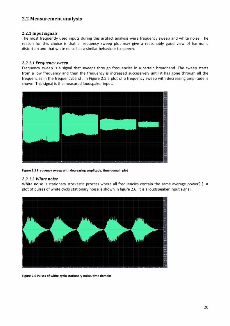
2.2.1.1 Frequency sweep Frequency sweep is a signal that sweeps through frequencies in a certain broadband. The sweep starts from a low frequency and then the frequency is increased successively until it has gone through all the frequencies in the frequencyband . In Figure 2.5 a plot of a frequency sweep with decreasing amplitude is shown. This signal is the measured loudspaker input.

Figure 2.5 Frequency sweep with decreasing amplitude, time domain plot

2.2.1.2 White noise White noise is stationary stockastic process where all frequencies contain the same average power[1]. A plot of pulses of white cyclo stationary noise is shown in figure 2.6. It is a loudspeaker input signal.

Figure 2.6 Pulses of white cyclo stationary noise, time domain

21

2.2.2 Hand held mode In the first graph that is shown in figure 2.7 the loudspeaker input is observed with a frequency sweep as an input. The signal has high amplitude. In figure 2.8 the microphone input is shown. If the two graphs are compared it is possible to distinguish two additional peaks that are shown in figure 2.8. The peaks are marked by red circles in the figure. Since the two additional peaks are multiples of the first peak, that could be seen to the left, they can be determined as harmonics.

In figure 2.9 and 2.10 the loudspeaker input and the microphone input are shown but this time with lower amplitude. If the two graphs are compared with the upper ones it could be seen that the peaks seems to be gone. Thus, the conclusion must be that the harmonic distortion is amplitude dependent for the hand held mode.

The input that is used for the third pair of graphs, 2.11 and 2.12, is white noise. Here is the harmonics not visible at all and this was not expected. This means that nonlinearities such as harmonic distortion are not visible for white noise input signal, which means that they are not present for speech signal either.

Figure 2.8 Microphone input. Frequency sweep with a high amplitude, frequency domain

Figure 2.7 Loudspeaker input. Frequency sweep with a high amplitude, frequency domain

Figure 2.9 Loudspeaker input. Frequency sweep with a low amplitude, frequency domain.

Figure 2.10 Microphone input. Frequency sweep with a low amplitude, frequency domain.

Figure 2.12 Microphone input. White noise, frequency domain

Figure 2.11 Loudspeaker input. White noise, frequency domain.

22

2.2.3 Hands free mode For these measurement settings and frequency sweep as an input the harmonic distortion is even more visible compared to the measurement with hand held mode, see figure 2.13 and 2.14. This may depend on the fact that the loudspeaker needs to generate a greater volume of the sound. This is because the communicator at the near-end must be able to understand the message from the far-end even though the mobile phone is placed on a distance from the near-end communicator.

In figure 2.15 and 2.16 the same input signal is illustrated as in figure 2.13 and 2.14 but with the difference that it has lower amplitude. Compared to the hand held mode where the harmonics were almost gone for the low amplitude signal the same relation is not found with the hands free mode. Here the harmonic distortion is almost the same for high and low amplitude inputs.

The result for the white noise input is the same for hands free mode as for hand held mode. This can be seen in figures 2.17 and 2.18.

Figure 2.12 Microphone input. Frequency sweep with a high amplitude, frequency domain

Figure 2.11 Loudspeaker input. Frequency sweep with a high amplitude, frequency domain

Figure 2.14 Loudspeaker input. Frequency sweep with a low amplitude, frequency domain

Figure 2.13 Microphone input. Frequency sweep with a low amplitude, frequency domain

Figure 2.16 Microphone input. White noise, frequency domain

Figure 2.15 Loudspeaker input. White noise, frequency domain

23

2.2.4 Measurement with an external microphone. To be sure that the harmonic distortion is not generated by the microphone on the mobile phone, measurements with an external microphone were performed. The result of this measurement is shown in figure 2.19 and 2.20. This measurement was done with hands free mode and the harmonics is still present in the microphone input signal. Thus, the conclusion is that the harmonics is not generated by the microphone in the mobile phone. Most likely the harmonics is generated by the loudspeaker.

2.3 Measurement result The purpose of the measurement was to distinguish the problem with nonlinear echo. The measurements were done with three different setups:

• Hand held mode

• Hands free mode • External microphone

From the measurement result, where frequency sweep is used as an input, it is seen that it is likely that harmonic distortion is causing the nonlinear echo. The harmonics is above all present in hands free mode when the loudspeaker needs to generate a loud volume sound, but it is also present to some extent for hand held mode when the input signal has high amplitude. Thus, for hand held mode the harmonic distortion is amplitude dependent, however this is not the case for the hands free mode.

Figure 2.20 Measured with an external microphone. Microphone input, frequency sweep, frequency domain

Figure 2.19 Measured with an external microphone. Loudspeaker input, frequency sweep, frequency domain

24

CHAPTER 3 POSSIBLE SOLUTIONS

25

3.1 Static method

3.1.1 Nonlinear loudspeaker effects The measurement described in chapter 2 clearly showed cheap loudspeakers used in mobile phones produce nonlinear effects where the major one is harmonic distortion. The static method estimates the harmonic distortion based on the loudspeaker input signal without considering the true residual echo as described in detail below.

3.1.2 Harmonic distortion The power of harmonics produced by loudspeakers depends on fundamental frequency and input signal power. Estimation of harmonic distortion in this implementation assumes that the loudspeaker output at frequency ;D contains the sum of the first six harmonic contributions from input frequencies below ;D which can be described as follows mathematically .

��de?��b�e�;X�� && \ & &&��gfdc�;X�� .&��g?g��gfdc�;X�� (3.1)

where ��de?��b�e�;X��&is loudspeaker output power at frequency ;X

Assuming the nonlinear power at ;X is only due to harmonic overtones:

��g?g��gfdc�;X�� $ _ ��dc�?g�e�;X �` . =�� Da (3.2)

The harmonic power is expressed in terms of linear power at fundamental frequency ;X as follows

��dc�?g�e�;X �` . =�� $&�D<�;X��gfdc�;X�� (3.3)

where ` $ =Y-Y[

Parameters used for the actual implementation of harmonic distortion estimation based on the above mathematical model are Harmonic Activation Level, Harmonic Gains, Fundamental Gain and Mapping table .

3.1.3 Harmonic Activation Level Harmonic Activation Level is the minimum loudspeaker input signal power above which harmonics will be produced. Hence if at any instant the loudspeaker input signal power is greater than Harmonic Activation Level, harmonics will be produced by the loudspeaker .

3.1.4 Harmonic Gains Harmonic Gains are defined as amplitude or power ratio of each of the six harmonics to the fundamental in dB scale.

�D $ -� �� i�k� Y&&&&&&&&&&&&&&` $ =Y-Y[ Y� (3.4)

where pD is amplitude of `b� harmonic signal. pX is amplitude of fundamental frequency

Harmonic Gain is used to calculate amplitude or power of harmonics produced for a given fundamental frequency .

26

3.1.5 Fundamental Gains Fundamental Gains describe the relative level of overtones produced by fundamentals in the frequency bands. Several tests for a specific loudspeaker are made to set a reasonable static Fundamental Gain describing how the overtones are emphasized in the frequency bands.

3.1.6 Mapping table The Mapping table is constructed based on the mathematical formula given in section 3.1.2 above to show which of the frequency bands below band k contributed harmonics that lie in band k.

3.1.7 Harmonic distortion estimation Estimation of harmonic distortion is implemented using the above parameters. First a regression variable is selected, either loudspeaker input signal or estimated echo. Then the power of the regression variable is compared with Harmonic Activation Level. If it is less than the Harmonic Activation Level then harmonics are not expected to be produced. Hence estimation will not be done. If it is greater than the Harmonic Activation Level then harmonics are expected to be produced and estimation of harmonics will continue. For a given regression variable input amplitude (or power), the first six harmonics amplitude (or power), are calculated from Harmonic Gains. The location of the frequency bands to hold these overtones and which harmonics should be added in a particular frequency band is determined by the mapping table. Then multiply the result by Fundamental Gain of each frequency band. The resulting estimated harmonic distortion is scaled by weights of linear echo estimator to track echo path effects of the harmonic distortion. Then the over all gain will be calculated based on the estimate of harmonic distortion. This gain is used to multiply the signal coming out of the linear AEC to reduce the non linear echo.

3.1.8 Mapping table construction In a banded frequency spectrum, identifying frequency bands those contributed overtones to the current band cannot be done by just dividing or multiplying the fundamental frequency as is the case with unbanded frequency bins. Instead a mapping table is constructed beforehand.

The current implementation divides the frequency spectrum into frequency bands; each with a bandwidth of 250Hz. If we consider a narrow band speech, the frequency extends to 4000Hz in which case the frequency spectrum will have 16 bands (4000Hz/250Hz). Table 3.1 shows 16 bands with their range of frequencies

Band Number

Minimum frequency

Maximum frequency

1 0 249 2 250 499 3 500 749 4 750 999 5 1000 1249 6 1250 1499 7 1500 1749 8 1750 1999 9 2000 2249 10 2250 2499 11 2500 2749 12 2750 2999 13 3000 3249 14 3250 3499 15 3500 3749 16 3750 3999

Table 3.1 Frequency bands for narrow band speech with their frequency range

27

To illustrate how the mapping table is constructed, calculation of the frequency bands which contribute overtones for the 6th band is described below. Calculate the harmonics for the 6th band:

1. Could the fundamental frequencies lie in band 6 for the 1st overtone?

à 1499 x 2 = 2998, 2998 > 1499 à No, the overtone will lie outside band 6 if that were the case. 2. Could the fundamental frequencies lie in band 6 for the 1st overtone?




à 500 x 2 = 1000, 1000 < 1449 à Yes, the overtone will lie inside band 6. 6. Could the fundamental frequencies lie in band 3 for the 2nd overtone?

à 500 x 3 = 1500, 1500 > 1449 à No, the overtone will lie outside band 6 if that were the case. 7. Could the fundamental frequencies lie in band 2 for the 2nd overtone?

à 250 x 3 = 750, 750 < 1449 à Yes, the overtone will lie inside band 6. 8. Could the fundamental frequencies lie in band 2 for the 3rd overtone?

à 250 x 4 = 1000, 1000 < 1449 à Yes, the overtone will lie inside band 6. 9. Could the fundamental frequencies lie in band 2 for the 4th overtone?


à 250 x 6 = 1500, 1500 > 1449 à No, the overtone will lie outside band 6 if that were the case. 11. Could the fundamental frequencies lie in band 1 for the 5th overtone?


à 1 x 7 = 7, 7 < 1449 à Yes, the overtone will lie inside band 6.

The result of the procedure for the 6th band will be as in Table 3.2. Overtone 1st overt. 2nd overt. 3rd overt. 4th overt. 5th overt. 6th overt. Multiple 2x 3x 4x 5x 6x 7x freq. band 3 2 2 2 1 1 Table 3.2 The result of calculating harmoincs for the 6th band

28

A full list of the overtones in each frequency band is shown in Table 3.3. Band Min freq Max freq h1 h2 h3 h4 h5 h6 1 0 249 1 1 1 1 1 1 2 250 499 1 1 1 1 1 1 3 500 749 2 1 1 1 1 1 4 750 999 2 2 1 1 1 1 5 1000 1249 3 2 2 1 1 1 6 1250 1499 3 2 2 2 1 1 7 1500 1749 4 3 2 2 2 1 8 1750 1999 4 3 2 2 2 2 9 2000 2249 5 3 3 2 2 2 10 2250 2499 5 4 3 2 2 2 11 2500 2749 6 4 3 3 2 2 12 2750 2999 6 4 3 3 2 2 13 3000 3249 7 5 4 3 3 2 14 3250 3499 7 5 4 3 3 2 15 3500 3749 8 5 4 3 3 3 16 3750 3999 8 6 4 4 3 3 Table 3.3 Complete mapping table

3.1.9 Summary The static method has low computational complexity and good performance in reducing non linear echo if reasonably accurate parameters are set for the particular mobile phone. The draw back of static method is measurements should be done for each cell phone to come up with parameters specific to the device. In addition to that, it computes the worst case scenario where it assumes if the harmonics are produced there will be maximum harmonic distortion all the time regardless of the amplitude or power of the loudspeaker input signal. This causes the overall gain calculation to be aggressive. Consequently it tries to remove more echo than what actually exists and this affects the near end speech.

29

3.2 Volterra filters

3.2.1 Introduction The Volterra series expansion was developed by the Italian mathematician Vito Volterra (1860-1940) in the 1880s. It is basically a generalization of Taylor series to accommodate memory. The idea of using Volterra series for filtering applications was introduced by Norbert Wiener (1894-1964) in the 1950s. Application of Volterra series for non linear system modeling is achieved by truncating the infinite series by considering only finite order and memory. Volterra filters are used in noise and echo cancellation, channel equalization, signal detection and estimation, spatial and temporal discrimination [15][16].

3.2.2 Mathematical description The Volterra series is defined as[6]:

�� $ X .& � �:�� % :��

�taX. � � ��:Y:�� %:�� % :�� .&[

�

�haX

�

�taX

.&_ _ [��haX��taX _ ��:Y:�Y [ Y:�� % :�� aX �� %:��[�� %:�� . u

(3.5)

where ��:Y:�Y [ Y:�� is Nth order kernel �� is the input and �� is the output

To model real systems the series is truncated in two ways: limiting the order of the kernel (N) and limiting the memory of the system to M.

The second order Volterra filter with memory M is shown below: �� $ X .&_ �:�� % :�¡@�taX ._ _ ��:Y:�� % :�� %:��¡@�haX¡@�taX

(3.6) An important property of the Volterra filter which minimizes the computational complexity significantly is the symmetry of its kernels. That is:

��:Y:�� $ ��:�Y:� (3.7)

Moreover the filter coefficients are linearly dependent which makes it suitable it for adaptive filter application, and hence on can use standard adaptive algorithms.

3.2.3 Adaptation of Volterra filters Volterra filter coefficients can be updated recursively using any adaptive algorithm since the error signal (difference between estimated and actual) can be written as a linear combination of the input signal to each filter coefficient [8][10]. Due it its ease of computation and fairly good convergence rate the LMS algorithm is widely used. Consequently its description for second order Volterra filter is discussed below.

30

First order Volterra kernel vectors: ¢�`� $ +��`�Y ��` % =�Y[ Y ��` %£ . =�,' ¤ $ +��Y�=�Y[ Y�£ % =�, Second order Volterra kernel vectors: ¢��`� $ & +��`�Y ��`��` % =�Y[ Y ��`��` %£ . =�Y ��` % =��` % =�Y[ Y ��` %£ . =��` %£ . =�,' ¤� $ +��Y��Y��Y=�Y [ Y��Y£ % =�Y��=Y=�Y[ Y��£ % =Y£ % =�, LMS adaptation is formulated as: ��`� $ X .&¤�`�¢�`� .&¤��`�¢��`� (3.8)

��`� $ ��`� % ��`� (3.9) X�` . =� $ &X�`� .&�X��`� (3.10) ¤�` . =� $ &¤�`� .&��`�¢�`� (3.11) ¤��` . =� $ &¤��`� .&��`�¢��`� (3.12)

where �XY �Y �� are step sizes for Volterra kernels and ��`� is the error.

The convergence speed of the LMS algorithm depends on the eigen vectors of the autocorrelation matrix of the input signal. The step size controls the speed of convergence and ensures stability of the filter.

3.2.4 Application of Volterra filter for Acoustic Echo Cancellation Adaptive Volterra filters are being applied for Nonlinear Acoustic Echo Cancellation (NAEC) purposes in hands-free communications due to the increased computational power of devices and low cost amplifiers and loudspeakers that introduce significant nonlinear echo. Efficiency of the overall AEC, both linear and nonlinear, depends on the ratio of linear to nonlinear echo signal power (LNLR). For high LNLR, linear echo dominates the nonlinear one in which case linear AEC is more efficient. Adding a Volterra filter in such scenarios will merely increase the computational complexity and possibly introduce gradient noise caused by the adaptation of higher order kernels. [17] LNLR is unknown at priori and will be time-varying for non-stationary signals like speech. Thus deciding either to use a simple linear filter or Volterra filter is difficult. Two types of filter combination methods are suggested in [17] to alleviate the problem. The first combines linear and Volterra filters, while the second method relies on the combination of kernels. Both methods perform at least as well as the best contributing filter.

3.2.5 Combination of Filters Scheme (CFS) A convex combination of an adaptive linear filter and adaptive Volterra filter including linear and quadratic kernel is considered as a possible solution for NAEC. Each filter independently updates its parameters using a separate adaptation step size and error signal power and then their output will be weighted by an adaptive parameter, �� , determining which output should be emphasized in the overall estimated echo signal. Pictorial description of the combination is shown in figure 3.1.

31

Figure 3.1 Combination of filters scheme

3.2.6 Description of the combination The outputs of the linear and Volterra filters can be computed as:

�� &$ ¥'��¢�� (3.13) �� $ ¤¦'��¢�� .&¢'��¤§��¢�� (3.14)

And the output of the combined filter is defined as: �� $ &�� . += % &��,��& (3.15)

where �� is an adaptive weighting parameter that controls the combination.

Better performance of the combination is achieved if each filter updates its parameters by its own rule[18]. Using standard gradient descent method for adaptation: ¥�� . =� $ ¥�� .&��¢�� (3.16)

¤¦�� . =� $ ¤¦�� .&��¢�� (3.17) ¤§�� . =� $ ¤§�� .&��¢��¢'�� (3.18)

where �� , �� and �� are step sizes and

�� $ &�� % �� (3.19)

�� $ &�� % ��& (3.20)

The weighting parameter �� can be updated in the same way with the intent of minimizing the error of the combined filter, i.e.

�� $ &�� % �� (3.21)

32

where �� is the output of the combined filter calculated in equation

Instead of adapting �� directly, [6] proposes adapting another parameter 4�� which defines �� as a sigmoidal activation function for the purpose of keeping ��&¨&��Y=� and to reduce gradient noise near �� $ = or �� $ �. [7] The weighting parameter is expressed as:

�� $ 3<:+4��, $ & ©= . �@d�g�ª@ (3.22)

Using the recently presented updating algorithm for 4�� and normalizing it for a better performance in case of time varying SNR:

4�� . =� $ 4�� .& «¬�g��+= % ��,��+�� % ��, (3.23)

where �� is an estimate of the power of +�� % ��, It is defined as:

�� $ n�� % =� .&�= % n�+�� % ��,� (3.24)

Therefore CFS works in such a way that when LNLR is low, there is high nonlinear echo, the Volterra filter represents an effective model of the channel, and minimization of the overall error yields �� ® � , so that �� ] ��&. The reverse occurs when LNLR is high with �� ® = and �� ] ��, so that the combination is equivalent to the linear filter avoid the gradient noise introduced by high order kernel of Volterra filter.

3.2.7 Combination of Kernels Scheme(CKS) This method tries to solve the problem by using only one Volterra filter and replacing one of its kernels by a convex combination of kernels, considering second order Volterra filter and replacing its quadratic kernel by two other kernels as shown in figure 3.2.

Figure 3.2 Simplified combination of kernels scheme

The output of the combination can be represented as:

33

�� $ ��D�� . &¯�� .&+= % ¯��,�� (3.25)

where ��D�� is the output of the linear kernel ��Y �� are the outputs of the kernels in the combination ¯�� is a mixing parameter in the range of (0,1)

For a better performance each kernel should update using its own adaptation rule and error signal, which allows the two replaced kernels to be different in any way, either in size or in memory. Letting the linear kernel adapt according to the overall error and each kernel according to its error signal, one has: �� $ &�� % �� (3.26)

�� $ &�� % +��D�� . ��, (3.27) �� $ &�� % +��D�� . ��,

Adaptation of the mixing parameter ¯�� is done by defining a sigmoid function as explained in CFS method above. Using Steepest Descent algorithm for its adaptation to minimize the overall squared error :

�� . =� $ �� .& «°�g�¯��+= % ¯��,��+�� % ��, (3.28)

where ¯�� $ 3<:+��,

A special case of the combination is when all taps of the first quadratic kernel are zero. �� $ ��D�� .& += % ¯��,�� (3.29)

This shows that the mixing parameter decides the role of quadratic kernel on the overall output of the kernel combination. Equation (13) can be written as: �� $ ¯��D�� .& += % ¯��,+��D�� .&��, (3.30)

Comparing equation (3.30) with equation (3.15) of CFS method, this method is only slightly more complex than the standard Volterra filter with addition of combining factor adaptation. It is better than the CFS method since it has only one linear filter while CFS updates two linear filters, one independent linear filter and the linear kernel of the volterra filter. Experiments with speech and colored input noise in [17] have shown that two methods, CFS and CKS, give a better result than only linear filter with up to 10dB Echo Return Loss Enhancement (ERLE) gain for high nonlinearity. Adaptation of the mixing parameter is very crucial since for a varying LNLR the ERLE improvement and complexity of algorithm are adjusted to be optimum by deciding whether kernels or filter should be given more emphasis for the overall output. Moreover, CKS is better than CFS for all LNLR scenarios providing less complexity and ERLE improvement.

3.2.8 Limitation of volterra filter Although Volterra filters can model a large class of nonlinear systems and its inherent property made it applicable for adaptive filter applications, it has some limitations which discourage its application for nonlinear systems:

1. High computational complexity for higher order nonlinear systems 2. Does not efficiently model strongly non linear systems 3. Slow convergence rate for non Gaussian inputs 4. Over-parameterization where large numbers of coefficient adaptations are needed even for low

order representations.

34

3.3 Hammerstein model

3.3.1 Introduction The (nonlinear) Hammerstein system is in resemblance with Volterra and Weiner (nonlinear) an advanced form of a nonlinear system. It consists of a series connection between a nonlinear and a linear block. The nonlinear block is static gain while the linear block is a dynamic system [19]. The blocks work together to build a model of the nonlinearities that e.g. is caused by the loudspeaker. There are two approaches of the Hammerstein model. The first approach assumes that the nonlinearities are of a polynomial kind so that the modelling could be divided into a linear and a nonlinear part. The second method does not assume that the model is polynomial all the time which makes it more difficult to create since it is necessary to make the estimation of a related function instead of the nonlinear elements. What these two methods have in common is that they create their model of a truncated series. The Hammerstein model in some cases has the capacity of creating dilated models of nonlinearities [21]. In the field of system identification the Hammerstein model has gained importance in areas like digital communication and biomedical engineering. In biomedical engineering it has been used to modelling muscle contractions [19]. System architecture

Figure 3.3 Nonlinear AEC – Hammerstein model (adaptive)

Figure 3.3 shows a proposition of the nonlinear part of an AEC Hammerstein model. The signal from the far-end is going through the nonlinear block first and then through the linear block. The blocks are modelling the acoustic echo and the noise that is captured by the microphone. The linear block will model the linear acoustic echo and the nonlinear block will model the nonlinear acoustic echo. The received signal will then be subtracted from the modelled noise and echo. After the subtraction the modelling blocks will be updated to improve future estimation [20].

35

EC = Encoder IFFT = Inverted Fast Fourier Transform + CP = Add the cyclic prefix D/A = Digital to analog converter PC = Physical channel A/D = Analog to digital converter SF = Shortening filter - CP = Remove the cyclic prefix FFT = Fast Fourier Transform DC = Decoder

3.3.2 AEC nonlinear Hammerstein design together with a shortening filter Like most nonlinear algorithms it brings high complexity and slow convergence. To overcome these issues the writers of article [20] propose an additional shortening filter. The idea is that the shortening filter will cut down the amount of taps needed in the linear block. Another benefit by adding the shortening filter is that the complexity of the updating algorithm to the AEC is reduced and that the grade of convergence will be improved [20]. The structure of the Hammerstein model together with a shortening filter can be seen in figure 3.4.

Figure 3.4 AEC nonlinear Hammerstein design together with a shortening filter

3.3.2.1 The shortening filter To avoid that two samples belonging to two different symbols will interfere with each other one has to make sure that there is enough distance between them. In a discrete multitone transceiver (DMT) this is done by a so-called cyclic prefix (CP) which is an intelligent guard time sequence. The CP adopts the distance between the samples from different symbols by calculating the length of the impulse response of an effective physical channel. Using a CP that is too long will decrease the capacity of the transceiver. To optimise the effective channel impulse response a shortening filter can be used to keep the length of CP short [21]. The shortening filter will contribute to minimise the length of the impulse response of the effective channel.

Figure 3.5 A illustration of the architecture of a shortening filter

36

In figure 3.5 there is a drawing of the structure of a shortening filter. Here follows an explanation of the flow in the figure. The bites that are coming from the far-end are transformed into carrier frequencies by the encoder. The carrier frequencies are converted to time-domain through the inverse Fast Fourier Transform. The cyclic prefix of a certain length is inserted between the symbols to make sure that samples of different symbols will not interfere. The signal is transformed from digital to analog throw the D/A converter and then transferred throw the physical channel where it is converted back to digital again by the A/D converter. The signal now passes through the shortening filter where the amount of taps is reduced. The next step is to remove the cyclic prefix and transform the signal into frequency domain by the Fast Fourier Transform. In the end of the process each frequency block is reconstructed into streaming bits in the decoder [21].

3.3.3 Mathematical representation

3.3.3.1 Initialization To create the Hammerstein model one starts with the initialization of some variables needed in the system. The signal from the far-end is denoted by p(n) and is branching in two directions; one where the signal is amplified and sent to the loudspeaker and the other one going to the AEC modelling. The filters that compose the AEC modelling are the nonlinear filter �� and the linear filter&��. The two filters are initialized as following: �� $ _ �D�D��&±Da Nonlinear modelling

�� $ ©�X��Y[ Y �²³@��ª' Linear modelling where ´� is the length of the linear filter. The nonlinear filter is composed by a linear combination of the nonlinear coefficient �&µ�¶&�·¸ basis function ��! They are denoted by: � $ +�Y ��Y [ Y �±,' Nonlinear coefficient

�� $ ©�x��yY ��x��yY [ Y �±x��yª' Basis functions And in matrix form �� $ ©�x��yY �x��yY [ Y �� % ´� . =�ª Matrix of the bias function where ´� is the length of the non linear filter. As could be seen in the figure above a signal is sent from the loudspeaker through the acoustic room and finally captured by the microphone. The signal from the microphone, which contains echo, noise and near-end speech, is denoted by y(n) in the figure and is initialized as follows: �� $ +��Y [ Y �� % ´¹ . =�,' Signal captured by the microphone Note that ´¹ is the length of the shortening filter.

3.3.3.2 The reference signals When the signal is sent through the first filter block from the far-field the following result is obtained: �� $ &�'�� (3.31) The next path the signal passes through is the linear filter. The reference signal that is given after the filter is: �� $ &�'�� $ &�'�� (3.32)

37

The signal that is captured by the microphone passes through the shortening filter and generates the following equation: �� $ & '�� (3.33)

3.3.3.3 The error signal Now one has reached the point where the signal from the loudspeaker through the shortening filter and the signal that has passed through the AEC path unite. The signal that has passed the echo path is now subtracted by the model which is illustrated in this equation:

�� $ �� % �� $ & '�� % �'�� (3.34)

3.3.3.4 Adaptation There are several adaptive algorithms that could be used to update the Hammerstein model. In the following text two of them are explained: LMS – adaptation �� . =� $ �� %&µº�� (3.35) �� . =�&updates the shortening filter by a subtraction of the product including the error signal and the signal captured by the microphone. µº denotes the step size of the adaptation of the shortening filter. �� . =� $ �� . µ��&�'�� (3.36) �� . =� updates the linear filter by adding the product of the error signal, the basis matrix and the nonlinear coefficients. µ� denotes the step size of the adaptation of the linear filter. �� . =� $ �� %&µ»�� (3.37) �� . =� updates the nonlinear filter by subtracting with the product including the error signal, the basis matrix and the value of the linear filter.&µ» denotes the step size of the adaptation of the nonlinear filter.

3.3.3.5 NLMS – adaptation Since the stability of the LMS adaptation cannot be ensured, the normalized LMS (NLMS) is introduced. The NLMS optimizes the value of the step size so that the adaptation algorithm both will be stable and ensure fast convergence.

3.3.3.6 Update for the shortening filter

�� . =� $ �� %&µ¼f�g�0�g��0�g��hh (3.38)

To improve the stability of the adaptation of the shortening filter the step size µº is divided by the microphone input&��. Update for the linear filter

�� . =� $ �� . µ¼f�g�&½¾�g�»�g��&½¾�g�»�g��hh

(3.39)

To improve the stability of the adaptation of the linear filter the step size µº is divided by the product of the bias matrix&�'�� and the nonlinear coefficient ��. Update for the nonlinear filter

38

�� . =� $ �� %&µ¿f�g�½�g��g��&½¾�g��g��hh (3.40)

To improve the stability of the adaptation of the nonlinear filter the step size µ» is divided by the product of the bias matrix&�'�� and the linear filter&�� [20].

3.3.4 Summary The Hammerstein model may be a good choice in the fields of digital communication and biomedical engineering. In good situations it may create a very accurate model of e.g. harmonic distortion. In resemblance with other nonlinear adaptive algorithms like the Volterra filter, it is computational complex and has slow convergence. According to article [20] these drawbacks could be overcome by adding a shortening filter to the Hammerstein filter architecture. It is shown in [20] that this new structure with the shortening filter uses less computational power and that the convergence speed is increased. One drawback to the addition of this shortening filter to the structure could be that the wanted signal becomes modulated in a way that could affect the sound. Thus, there could be a change in the voice characteristics. The writers of article [20] recommend using an equalizer to compensate for this problem. Double talk, that is, when two persons that communicate through the phone talk at the same time, is an issue for most adaptive algorithms that deals with AEC. Unfortunately the Hammerstein model is not an exception. When double talk occurs, the algorithms have difficulties to decide what is echo and what is near-end speech. This will result either in that the near-end speech will be destroyed or that enjoying echo will be let through to the other end. One solution to this problem can be to make the algorithm adapt slower when there is double talk or even stop adapting during this time. This solution requires that the algorithm has access to a double talk detector [20].

39

3.4 Harmonic distortion residual echo suppressor (HDRES)

3.4.1 Introduction The method of “Nonlinear Residual Acoustic Echo Suppression for High levels of Harmonic Distortion” [22] have been developed by Diego A. Bendersky from the University of Buenos Aires and Jack W. Stokes, Henrique S. Malvar from Microsoft Research. Although there are many methods that can reduce the influence of nonlinear echoes and still keep a good quality of the near end speech, not so many of them are suitable when it comes to hand held devices. Volterra filters and neural networks for example involve complex calculation and use many variables which results in slow convergence and higher computational complexity. A better way to speed up the convergence and minimize the computational could be to use a residual echo suppressor, also called RES. The RES works together with the linear AEC and contributes to the cancelation of the harmonic distortion (HD). Thus, the full name of this algorithm becomes Harmonic Distortion Residual Echo Suppression (HDRES). Figure 3.6 illustrates in a simplified way how the HDRES and the linear AEC filter are working together to cancel the echo. The trick that the HDRES uses is that it lets the linear AEC cancel as much of the echo as possible with the magnitude and the phase, and then the HDRES will suppress the nonlinear echo further. The HDRES algorithm that works in the frequency domain will not use so much computational capacity since it only calculates a single transform from the speaker signal at the time [22].

Figure 3.6 A simplified illustration of how the HDRES and the linear AEC works together

3.4.2 Residual echo suppression (RES) The limitation of the linear acoustic echo canceller to subtract nonlinear echo from the echo path have created a need of an external box that could deal with this issue. The residual echo suppressor is an additional tool to suppress the nonlinear echo while still keeping the speech signal intact [24]. One condition for the RES to work is that the real signal that has its origin from the loudspeaker through the echo path and into the microphone needs to be separated from the estimated signal from the adaptive filter. To be able to do this the signal is divided into blocks in suitable sizes. The block is converted into the frequency domain through a filter bank or a discrete Fourier transform (DFT). The RES relies on a model of the nonlinear echo created in frequency domain.

3.4.3 System architecture This acoustic echo cancelation system consists of two different filters. One of the filters is intended to cancel the linear echo and the other one will suppress the nonlinear echo. The first filter is a linear AEC adaptive algorithm that is working in the frequency domain. The second filter is the HDRES filter and it is also working in the frequency domain. Those two filters are parallel coupled with each other, this is illustrated in figure 3.7. The transformation from the time domain to the frequency domain is done by a modulated complex lapped transform (MCLT) [23].

40

3.4.4 Modulated Complex Lapped Transform (MCLT) Since the HDRES algorithm is doing its arithmetic operations in the frequency domain the loudspeaker signal, that is in time domain, needs to be converted. There are many ways to convert a time domain signal into frequency domain. One possible method is to use discreet Fourier transform DFT and another method is Modulated Complex Lapped Transform, MCLT [3]. The MCLT is a complex version of the modulated lapped transform, MLT. The MLT is often used together with a system which contains noise reduction or acoustic echo cancelation, since it has perfect reconstruction. The perfect reconstruction minimizes the disturbances that other time-frequency converters are struggling with [24]. The MLT is developed from a cosine modulated filter bank which is modulating by cosines instead of exponentials. This means that it will generate two frequency shifts instead of one since the cosine is a summation of two exponentials [2]. The MLT is working with real numbers and therefore it has a limitation when it comes to working the system which contains complex information like the phase. Thus, the MLT is not suitable for systems that deal with noise subtraction and acoustic echo cancelling. To be able to use the MLT in those areas Henric Malvar on Microsoft research has developed an improved version of the MLT that also can work with complex numbers. Because of this extension the MCLT could be a good alternative to the standard DFT filter banks in areas like noise suppression and AEC. In the article [24] it is shown that the MCLT produce fewer disturbances during the convergence time to frequency domain or vice versa than the DFT filter bank [24].

Figure 3.7 Illustrates the architecture of the HDRES model together with a linear AEC. A explanation of the notation is shown below

3.4.5 Mathematical representation

3.4.5.1 The linear filter The linear filter estimates the loudspeaker signal that is travelling through the echo path by calculating a summation of the product of the complex weight À² and the loudspeaker signal&� [22]. Thus, the

estimated echo � is represented by:

� ��Y:� $ &_ À²�6Y:�'@baX �� % 6Y:� (3.41)

41

In this function the number of taps, [t=?], frame index and the frequency band are represented by T, t, n, m respectively. The echo subtraction can be represented by the equation:

(��Y:� $ & G��Y:�G %&Á� ��Y:�Á (3.42) Here the real echo is subtracted by the estimated echo. After the subtraction the linear AEC filter is updated so that the estimation can be improved.

3.4.5.2 The HDRES filter The HDRES filter is suppressing the nonlinear echo by the multiplication of a constant, which has a value between 0 and 1, and the output from the linear AEC. The constant which is multiplied is called the gain � and is calculated by taking the maximum value between the noise floor Â and the input ( (output to the linear AEC) subtracted by the residual echo �c multiplied with a constant factor β, which determines the aggressiveness of the equation. The maximum value is subtracted by the input (!

��Y:� $ &�d1)ÃÄ�gY��@mÅÄÆ�gY��Y�Ç�gY��&*ÃÄ�gY�� (3.43)

The additional bar on top of the letters E, �c and Â means that their magnitude is smoothed. This is done through the following calculation. (Ä��Y:� $ & �= % &È�(Ä�� % =Y:� . ÈG(��Y:�G (3.44)

�Äc��Y:� $ & �= % &È��Äc�� % =Y:� . ÈÁ�cÉ ��Y:�Á (3.45) ÂÇ��Y:� $ & �= % &È�ÂÇ�� % =Y:� . ÈÁÂÉ��Y:�Á (3.46)

α makes it possible to decide how much of the functions that should be smoothed. �cÉ ��Y:� denotes the estimated residual echo and is used to model the residual echo that is passed through the linear AEC. The model consists of a mapping of the spectral power, parameters of the HDRES model and the loudspeaker input in frequency domain. � c��Y:� $ &_ _ _ Ê�2Y ËY `Y:�±Da@± ÀU�2Y ËY `�G�Ì��Y 2�GoÍa¡�a (3.47)

Ê�2Y ËY `Y:� $ & Î=&&&&&&&&&&&&&&&&&&&2;&2&�&Ë . ` $ :�&&&&&&&&&&&&&&&&&&&&&&&&&&&&&&76��823�Ï (3.48)

The model is used for modulating the harmonic distortion of the sound from the loudspeaker which is caused by the loudspeaker itself. The harmonics are multiples of the fundamental frequency. So if the fundamental frequency is f then the second harmonic will appear at two times the fundamental frequency (2f), the third harmonic will appear at three times the fundamental frequency (3f) and so forth. In the model we find&£, � and Ð which are representing the number of subbands, the number of harmonics which are considered and the echo leakage respectively. To avoid the echo leakage it is recommended to set&Ð $ =. The fundamental frequency of the signal in this model is denoted as 2 and the actual number of harmonics is symbolized by&Ë. ` is the index of the harmonic search window [22]. Ê�2Y ËY `Y:� is used to decide which band the harmonics will end up in. ÀU�2Y ËY `� is a part of the HDRES model and �Ì��Y 2�& is a delayed version of the speaker signal. To be able to make an estimation of the nonlinear echo the loudspeaker and the residual echo needs to be correlated. The correlation calculation complicates by the time delay that arises from the sound waves travelling through the echo path. To be able to handle this problem the regression is computed through a normalised transformation predicated by a delayed version of the speaker signal,&G�Ì��Y:�G. It is calculated as follows: �Ñ��Y:� $ &_ ´�6Y:�G�� % 6Y:�G'@baX (3.49)

42

´�6Y:� is the normalized weighting factor and � is the speaker signal. Thus �Ñ��Y:� becomes weighted with linear AEC tap weights. The normalised weighting factor is determined by the weighting matrix that is calculated in the linear acoustic echo canceller.

´�6Y:� $ & GÒÓ�bY��G_ GÒÓ�ÍY��G¾stÔjk (3.50)

To be able to continuously follow the development of the Harmonic distortion of the loudspeaker signal the HDRES need to be updated after each calculation. This can be done with any linear adaptive algorithm. In [22] this is done by a normalized LMS algorithm.

ε��Y:� $ G(��Y:�G %& Á� c��Y:�Á (3.51) ÀU�2Y ËY `� $ &ÀU�2Y ËY `� .& µ

Õ�gY��ÄÄÄÄÄÄÄÄÄÄ�Ñ��Y:�ε��Y:� (3.52)

As could be seen in the equations above, the error signal is calculated by a subtraction between the input of the linear AEC, &(��Y:�, and the residual echo estimation&�Éc��Y:�. The error signal ε��Y:� is then used to make a better estimation of the echo in the next calculation of the HDRES model quantity&ÀU�2Y ËY `�. The step size µ&is used to set how fast the algorithm should converge. To make the algorithm more stable, the NLMS algorithm including a division of the average power of the speaker signal [22]. This is calculated by: ÖÄ�� . =Y:� $ & �= % ρ�ÖÄ��Y:� . ρG�Ñ��Y:�G� (3.53)

3.4.6 Summary The HDRES algorithm is a good choice when it comes to low usage of the computational capacity and fast convergence. It is therefore more suitable for hand held devices compared to other nonlinear echo cancellers in those aspects. According to the articles and [9] the RES algorithm has shown good performance to cancel nonlinear artefacts produced by the loudspeaker. However, the HDRES has a disadvantage similar to many other adaptive algorithms that is used for acoustic echo cancelling, and that is sensitivity for double talk. This means that if a near-end speech is present at the same time as the updating of the HDRES filter, a considerably amount of the near-end speech will be destroyed. The writers of the article [22] suggest a possible way to overcome this drawback. The idea is to go back a number of adaption steps when doubletalk occurs. That way the last adaptation step that did not include any near-end speech could be used and the near-end speech will not be destroyed. This solution requires that the algorithm has access to a double talk detector [22]. Benefits/drawbacks of the method: Benefits:

• Low complexity • Fast convergence

• Small use of the computational capacity

• Suitable for hand held devices

Drawbacks • Sensitive to doubletalk

43

CHAPTER 4 IMPLEMENTATION

44

4.1 Implementation in Matlab

4.1.1 Summary of the four methods As stated above, the purpose of this thesis is to investigate different methods that deal with nonlinear acoustic echo cancelation. The four methods that were chosen to be investigated more closely are the Static method, Volterra filter, the Hammerstein model and HDRES. These methods were chosen because they represent a few of the most promising methods to cancel nonlinear echo. The static method has low computational complexity and since it is not adapting it has low computer power consumption. The drawback of using a static mehod is that adjustments have to be done for each mobile phone where it is implemented. The method might also remove more echoes than actually exist since it always models the worst case. The Volterra filter represents the general nonlinear modelling. The method has existed for a long time and is regarded reliable. It can model a large class of nonlinear system and has properties that are suitable for AEC. The drawbacks of this method is that it has high complexity and slow convergence. The Hammerstein model has similar properties to the Volterra filter and in some situations has the capacity to create a very accurate model. In resemblance with Volterra it demands high computational complexity and slow convergence. The HDRES model is different from the other models in that it is working in the frequency domain instead of in the time domain. This condition along with other adjustments gives this method other properties than the others, e.g. low computational complexity and fast convergence. These properties makes it more suitable for hand held devices and therefore is the first choice. However, all these methods have a problem with sensitivity to double talk. This property seems to be consistent for most methods that deal with nonlinear acoustic echo cancellation according to our study. Thus, the HDRES model is chosen to be the main focus area from this point. The next step is to start the implementation of the selected method. The idea is to first implement the algorithm in Matlab, where it will be tested and analysed, and when it is good enough it will be converted to C. A flow chart of the HDRES algorithm is found in figure 4.1.

4.1.2 Changes from the article The article “Nonlinear Residual Acoustic Echo Suppression for High levels of Harmonic Distortion” [22] that has been written by Diego A. Bendersky from the University of Buenos Aires and Jack W. Stokes, Henrique S. Malvar from Microsoft Research works as a template for the present implementation. Their method for nonlinear acoustic echo cancelation was developed for use in laptop computers. The intention of this study is to adjust the method to make it more suitable for hand held devices such as cell phones. The difference of implementing the HDRES method for use of a cell phone compared to a laptop computer is the amount of computer power that is available. In the HDRES article, calculation for harmonics is done for every frequency bin but in the present implementation this is done for every frequency band. The reason is that the algorithm will use less computer power. The drawback of this change is that the accuracy of the method will decrease. Another difference in the present implementation compared to the article is that instead of modulated complex lapped transform the Fast Fourier Transform (FFT) is used to go from time domain to frequency domain. This change is made to make the environment in Matlab, during the testing, similar to the one where it is going to be implemented in C later on.

45

Figure 4.1 Flowchart of the HDRES model

4.1.3 Additional changes from development During the development of the HDRES algorithm two more improvements were done, averaging and limiting of the weights. The averaging was done for every block to improve the stability of the algorithm. The reason for limiting the weights was stopping the algorithm from moving more energy to another band than what is possible for a real signal with harmonics. Matlab – description of the code

4.1.4 Frequency banding The banding takes the sum of eight frequency bins and put them into one frequency band. It considers FFT transformed values from 1 to N/2 to avoid redundancy, were N is size of the FFT. Extract of the Matlab code is shown in Table 4.1.

46

Table 4.1 Extract of the Matlab code for the calculation of the frequency band

4.1.5 Call for the mapping matrix Table 5 shows a function call of the mapping matrix (MappingMatrix) function. The function has four inputs: The number of harmonics, the echo leakage, the frequency band size and the sampling frequency. The function itself is described in detail in the section of the mapping matrix. Extract of the Matlab code is shown in Table 4.2. Table 4.2 Extract of the Matlab code for the call of the mapping matrix

4.1.6 Estimation The calculation of the estimation is made by using the mapping matrix function which calculates which bands the harmonics are in. For those cases the estimation parameter is updated by a product of the weighting function and the loudspeaker input. An extract of the Matlab code is shown in Table 4.3. Table 4.3 Extract of the Matlab code for the calculation of the estimation. M, m, H and L are number of frequency band, fundamental frequency band, number of harmonics and echo leakage respectively

for m = 1:M temp = 0; for i = 1:m for j = 1:H for l = -L:L if (MappingMatrix(m,i,j,l+(L+1)) == 1) temp = temp + WR(m,i,j,l+(L+1))*Xprimek_masked(i); end end end end Drhatk(m) = temp;

MappingMatrix = CalculateFreqBandMapping(H,L,fs/2/M,fs);

for fb = 1:8:N/2 Xk(ceil(fb/8)) = sum(abs(Xktemp(fb:fb+7)).^2); Drk_ref(1,ceil(fb/8)) = sum(abs(Drktemp(fb:fb+7)).^2); end

47

Improvements during development:

4.1.7 Averaging To compensate for the effects from the banding, averaging is used. Averaging is calculated by taking the previous spectrum added with the present spectrum and then dividing the sum with two. Extract of the Matlab code is shown in Table 4.4. Table 4.4 Extract of the Matlab code for the averaging calculation

4.1.8 Limiting the weights This function has the purpose of limiting the weight so that more power than actually is the case for the harmonics is not transferred to the band. In the C implementation the weight limit (WeightLimit) is changed to the relative gain (Rg), which is the ratio between the gain of the fundamental and the harmonics. Extract of the Matlab code is shown in Table 4.5. Table X. Extract of the Matlab code for the weigh limiting calculation.

Table 4.5 Limiting the weights

4.1.9 The MappingMatrix function The purpose of the MappingMatrix function is to determine what bands the harmonics may end up in for a certain frequency. The MappingMatrix is a three-dimensional matrix and each dimension can be divided into fundamental frequency, band number and number of harmonics. It includes all information about the overtones. The information is stored as ones and zeros in the matrix. In Table 4.6 the Matlab code is included that calculates the MappingMatrix. Table 4.6 A part of the Matlab code that calculated the MappingMatrix

Thus, the MappingMatrix can be divided into X two-dimensional slices, where X stands for the number of overtones (harmonics) considered. The first overtone can be considered as an example: A table of the first overtone is shown in figure 4.2. The element which is denoted by one has the meaning that for that

if k == 1 drk=dr(k:k+79); else drk=(dr(k-80:k-1)+dr(k:k+79))/2; end

if WR(m,i,j,l+(L+1)) > WeightLimit WR(m,i,j,l+(L+1))= WeightLimit; end

for i = 1:NbrFreqBands for j = 1:NbrHarmonics LowestBand = floor(FreqLowLimit(i)*j/Bandwidth); HighestBand = floor(FreqHighLimit(i)*j/Bandwidth); BandNumberIndex = (LowestBand:1:HighestBand)+1; BandNumberIndex = BandNumberIndex(find(BandNumberIndex <= NbrFreqBands)); BandNumberIndex = BandNumberIndex(find(BandNumberIndex >= 1)); MappingMatrix(BandNumberIndex,i,j) = 1; end end

48

fundamental frequency the overtone can exist in the corresponding band, e.g. A1 in the table is denoted by 1. That means that if the fundamental frequency lies between 0 and 249 Hz the first overtone may only exist in the first band. For the second overtone, see figure X, there are ones in both A1 and A2. This means that if the fundamental frequency lies between 0 and 249 Hz the second overtone may only end up in the first or the second frequency band. If six harmonics is considered there will be six tables like the ones which are shown in figure 4.2 and 4.3. The mathematical explanation of this behavior is the following:

4.1.10 Mathematical explanation If the second overtone is considered and the fundamental frequency lies somewhere between 250 and 499 Hz there may be a fundamental frequency at 300 Hz in that range which may generate a second overtone at Z��&� w - $ &&��&� . Thus a second overtone may lie in band 3. If instead a fundamental frequency that has a value of 400 Hz is considered, still in the same range, the second overtone may end up in ×��&� w - $ &&Ø��&� . Thus, the second overtone may also end up in the forth band. Compare this result with figure 4.2. First overtone:

Fundamental frequency

A B C D E F G H I J K L M N O P

Freq

uenc

y ba

nds

1 1 0 0 0 0 0 0 0 0 0 0 0 0 0 0 0 2 0 1 0 0 0 0 0 0 0 0 0 0 0 0 0 0 3 0 0 1 0 0 0 0 0 0 0 0 0 0 0 0 0 4 0 0 0 1 0 0 0 0 0 0 0 0 0 0 0 0 5 0 0 0 0 1 0 0 0 0 0 0 0 0 0 0 0 6 0 0 0 0 0 1 0 0 0 0 0 0 0 0 0 0 7 0 0 0 0 0 0 1 0 0 0 0 0 0 0 0 0 8 0 0 0 0 0 0 0 1 0 0 0 0 0 0 0 0 9 0 0 0 0 0 0 0 0 1 0 0 0 0 0 0 0 10 0 0 0 0 0 0 0 0 0 1 0 0 0 0 0 0 11 0 0 0 0 0 0 0 0 0 0 1 0 0 0 0 0 12 0 0 0 0 0 0 0 0 0 0 0 1 0 0 0 0 13 0 0 0 0 0 0 0 0 0 0 0 0 1 0 0 0 14 0 0 0 0 0 0 0 0 0 0 0 0 0 1 0 0 15 0 0 0 0 0 0 0 0 0 0 0 0 0 0 1 0 16 0 0 0 0 0 0 0 0 0 0 0 0 0 0 0 1

Figure 4.2 Table of the mapping matrix for the first overtone

A & 1: 0 - 249 Hz B & 2: 250 - 499 Hz C & 3: 500 - 749 Hz D & 4: 750 - 999 Hz E & 5: 1000 - 1249 Hz F & 6: 1250 - 1499 Hz G & 7: 1500 - 1749 Hz H & 8: 1750 - 1999 Hz I & 9: 2000 - 2249 Hz J & 10: 2250 - 2499 Hz K & 11: 2500 - 2749 Hz L & 12: 2750 - 2999 Hz M & 13: 3000 - 3249 Hz N & 14: 3250 - 3499 Hz O & 15: 3500 - 3749 Hz P & 16: 3750 - 3999 Hz

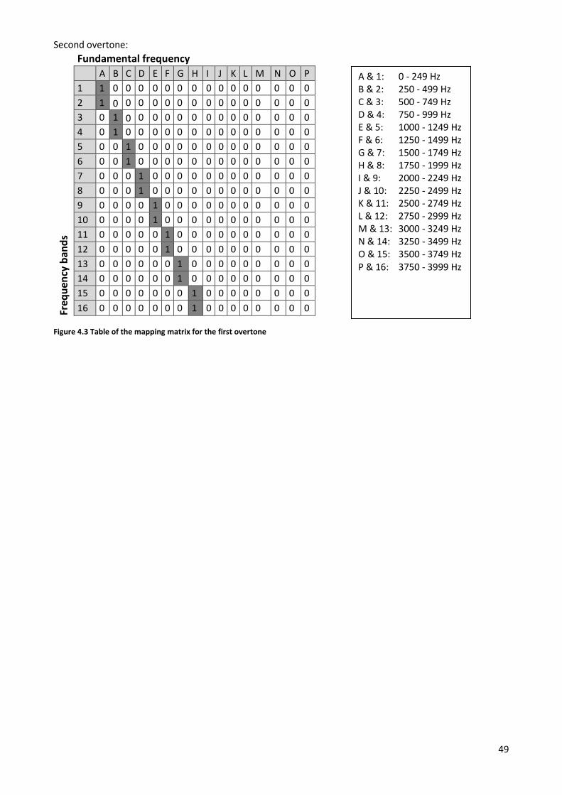
49

Second overtone:

Fundamental frequency

A B C D E F G H I J K L M N O P

Freq

uenc

y ba

nds

1 1 0 0 0 0 0 0 0 0 0 0 0 0 0 0 0 2 1 0 0 0 0 0 0 0 0 0 0 0 0 0 0 0 3 0 1 0 0 0 0 0 0 0 0 0 0 0 0 0 0 4 0 1 0 0 0 0 0 0 0 0 0 0 0 0 0 0 5 0 0 1 0 0 0 0 0 0 0 0 0 0 0 0 0 6 0 0 1 0 0 0 0 0 0 0 0 0 0 0 0 0 7 0 0 0 1 0 0 0 0 0 0 0 0 0 0 0 0 8 0 0 0 1 0 0 0 0 0 0 0 0 0 0 0 0 9 0 0 0 0 1 0 0 0 0 0 0 0 0 0 0 0 10 0 0 0 0 1 0 0 0 0 0 0 0 0 0 0 0 11 0 0 0 0 0 1 0 0 0 0 0 0 0 0 0 0 12 0 0 0 0 0 1 0 0 0 0 0 0 0 0 0 0 13 0 0 0 0 0 0 1 0 0 0 0 0 0 0 0 0 14 0 0 0 0 0 0 1 0 0 0 0 0 0 0 0 0 15 0 0 0 0 0 0 0 1 0 0 0 0 0 0 0 0 16 0 0 0 0 0 0 0 1 0 0 0 0 0 0 0 0

Figure 4.3 Table of the mapping matrix for the first overtone

A & 1: 0 - 249 Hz B & 2: 250 - 499 Hz C & 3: 500 - 749 Hz D & 4: 750 - 999 Hz E & 5: 1000 - 1249 Hz F & 6: 1250 - 1499 Hz G & 7: 1500 - 1749 Hz H & 8: 1750 - 1999 Hz I & 9: 2000 - 2249 Hz J & 10: 2250 - 2499 Hz K & 11: 2500 - 2749 Hz L & 12: 2750 - 2999 Hz M & 13: 3000 - 3249 Hz N & 14: 3250 - 3499 Hz O & 15: 3500 - 3749 Hz P & 16: 3750 - 3999 Hz

50

4.1.11 Matlab results

4.1.11.1 The input signal The input signal which was generated in Matlab consists of a fundamental and a number of harmonics. By letting the fundamental frequency and the number of harmonics vary, the performance of the HDRES algorithm could be tested. The amplitude of the harmonics varies randomly but the amplitude for harmonics higher than three is significantly lower than the others. This was done to create a more realistic input signal. An example of the input signal can be observed in figure 4.4.

Figure 4.4 The input signal created for testing of the HDRES algorithm in Matlab

4.1.11.2 Estimation To be able to cancel the harmonic distortion of the loudspeaker signal it must be estimated. In figure 4.5 and 4.6 the true residual echo and the estimated residual echo is presented. A comparison between the two figures shows that they are similar except for the first frequency band. The reason why the first band is not estimated is that there are no harmonics there for this case. Thus, the estimation of the harmonic distortion seems to be fairly good, at least for this kind of input signal. This result is important for the continuing implementations in C since the estimation part is one of the major parts that are going to be implemented in the AEC structure.

51

Figure 4.5 Plot of the true residual echo

Figure 4.6 Plot of the estimate of the true residual echo

4.1.11.3 The error function To be able to rate the performance of the estimation the error signal can be used. The error function specifies the difference between the true signal and the estimate. Thus, the lower value of the error function the better is the estimation. The figure 4.7 shows a plot of the error function for the true residual echo and its estimation. The error function is made for one chosen band.

52

Figure 4.7 The error function, gives the difference between the true residual echo and its estimation

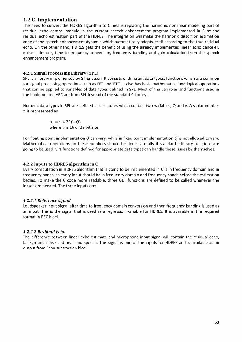
53

4.2 C- Implementation The need to convert the HDRES algorithm to C means replacing the harmonic nonlinear modeling part of residual echo control module in the current speech enhancement program implemented in C by the residual echo estimation part of the HDRES. The integration will make the harmonic distortion estimation code of the speech enhancement dynamic which automatically adapts itself according to the true residual echo. On the other hand, HDRES gets the benefit of using the already implemented linear echo canceler, noise estimator, time to frequency conversion, frequency banding and gain calculation from the speech enhancement program.

4.2.1 Signal Processing Library (SPL) SPL is a library implemented by ST-Ericsson. It consists of different data types; functions which are common for signal processing operations such as FFT and IFFT. It also has basic mathematical and logical operations that can be applied to variables of data types defined in SPL. Most of the variables and functions used in the implemented AEC are from SPL instead of the standard C library. Numeric data types in SPL are defined as structures which contain two variables; Q and v. A scalar number �&is represented as �& $ C w -Ù�%��

where C is 16 or 32 bit size.

For floating point implementation � can vary, while in fixed point implementation � is not allowed to vary. Mathematical operations on these numbers should be done carefully if standard c library functions are going to be used. SPL functions defined for appropriate data types can handle these issues by themselves.

4.2.2 Inputs to HDRES algorithm in C Every computation in HDRES algorithm that is going to be implemented in C is in frequency domain and in frequency bands, so every input should be in frequency domain and frequency bands before the estimation begins. To make the C code more readable, three GET functions are defined to be called whenever the inputs are needed. The three inputs are:

4.2.2.1 Reference signal Loudspeaker input signal after time to frequency domain conversion and then frequency banding is used as an input. This is the signal that is used as a regression variable for HDRES. It is available in the required format in REC block.

4.2.2.2 Residual Echo The difference between linear echo estimate and microphone input signal will contain the residual echo, background noise and near end speech. This signal is one of the inputs for HDRES and is available as an output from Echo subtraction block.

54

4.2.2.1 Noise estimate Background noise estimate is the third input for HDRES. It will be used to remove background noise from the output of echo subtraction block so that the algorithm will estimate residual echo only, instead of their sum. Noise estimation is done in noise reduction block. Hence the estimate is extracted from this block.

4.2.3 HDRES algorithm in C The HDRES function definition is given below:

void HDRES(SPL_vint32Q_t* SPL_Drhatk,double* Xprimek1,double* Ek1,double* Nk1,HDRES_DATA* HData)

The function has five arguments where SPL_Drkhatk is used as output of the function which holds residual echo estimate. Xprimek1 is the loudspeaker input signal. Ek1 is the difference between the echo estimate and microphone input signal. Nk1 is the noise estimate and HData contains previous values of variables that will be used in the algorithm.

Data type of the first argument and last arguments are pointers to structures defined by the key word struct in C programming while the rest are pointers to double. The body of the HDRES algorithm in C is very similar to the MATLAB except some syntax changes. The major differences were:

• Variables should be declared and initialized before they are used in the case of C which was not the case in MATLAB.

• Copying values into vectors should be done by loops in C where a simple equal sign was enough in MATLAB if the vectors have equal size.

Residual echo estimation code in C is given in Table 4.7 to compare it with the MATLAB code given above.

Table 4.7 Residual echo estimation

The weight updating code in C as shown in Table 4.8 is not allowed to update weights all the time. The algorithm is allowed to update if the weight is less than the possible limit provided in vector Rg(Relative gain). Otherwise the maximum possible value given in Rg will be set. Relative gain is set by customers by measuring the ratio of power of overtones to power of the fundamental frequency. Implementing this condition check will guarantee that no power is transferred to a band by the loudspeaker more than is physically possible.

for (m = 0; m < M; m++){ temp = 0; for (i = 0; i < m; i++){ for (j = 0; j < H; j++){ if (MappingMatrix[m][i][j] == 1)

{ temp = temp + currentWR[m][i][j]*Xprimek_masked[i];

} } }

Drhatk[m] = temp; }

}

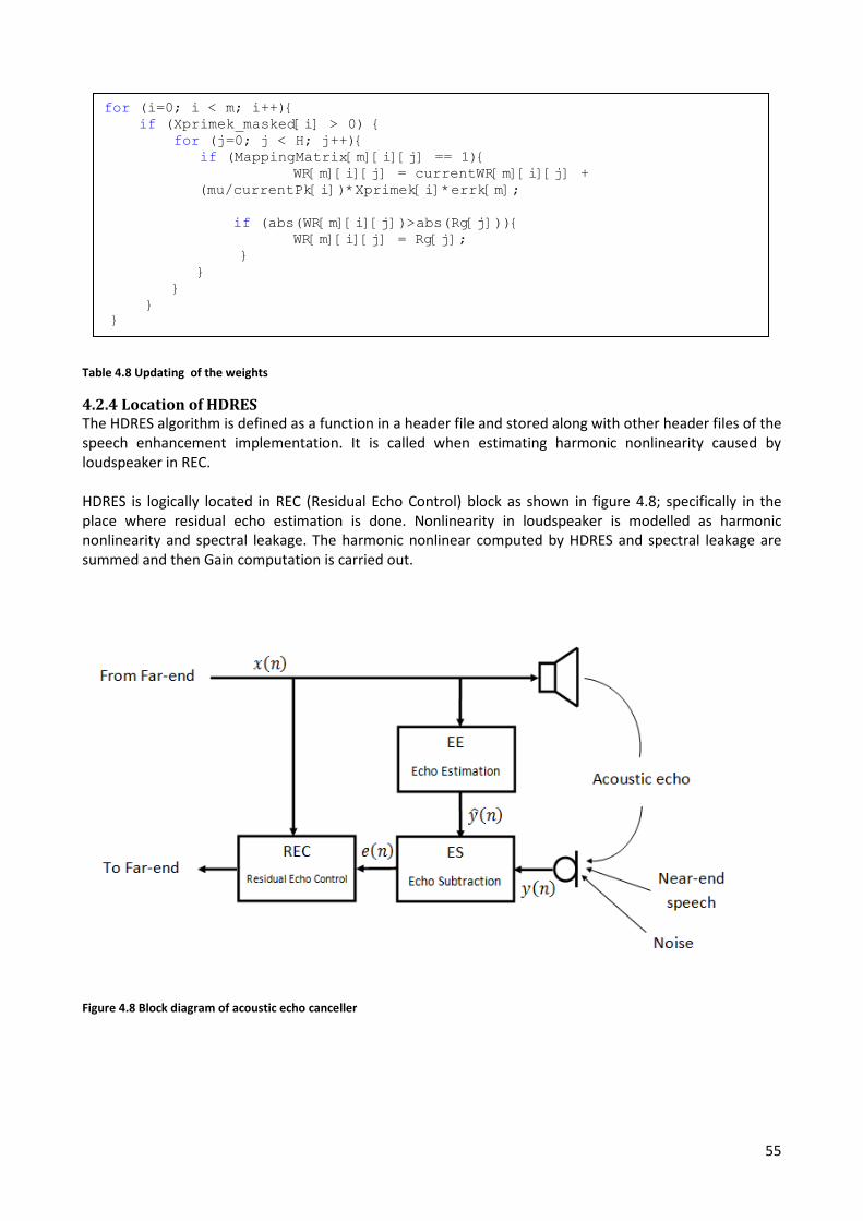
55

Table 4.8 Updating of the weights

4.2.4 Location of HDRES The HDRES algorithm is defined as a function in a header file and stored along with other header files of the speech enhancement implementation. It is called when estimating harmonic nonlinearity caused by loudspeaker in REC. HDRES is logically located in REC (Residual Echo Control) block as shown in figure 4.8; specifically in the place where residual echo estimation is done. Nonlinearity in loudspeaker is modelled as harmonic nonlinearity and spectral leakage. The harmonic nonlinear computed by HDRES and spectral leakage are summed and then Gain computation is carried out.

Figure 4.8 Block diagram of acoustic echo canceller

for (i=0; i < m; i++){ if (Xprimek_masked[i] > 0) { for (j=0; j < H; j++){ if (MappingMatrix[m][i][j] == 1){

WR[m][i][j] = currentWR[m][i][j] + (mu/currentPk[i])*Xprimek[i]*errk[m];

if (abs(WR[m][i][j])>abs(Rg[j])){

WR[m][i][j] = Rg[j]; } } } } }

56

4.2.5 Output of HDRES

Output of HDRES in C is estimated residual echo in frequency domain and frequency banded. Moreover the datatype should be converted to SPL; a code that converts residual echo estimate stored in double vector Drkhatk to SPL type is given in Table 4.9.

Table 4.9 Double to SPL type conversion

SPL_vint32Q_t* SPL_Drhatk; SPL_Drhatk->Q = 0;

SPL_Drhatk->L = 16; SPL_Drhatk->v_p = Drhatk;

57

CHAPTER 5 RESULTS

58

5.1 Introduction In summary, the article about an algorithm called “Harmonic Distortion Residual Echo Cancelation” written by Diego A. Bendersky, Jack W. Stokes and Henrique S. Malvar was chosen for further investigation. The algorithm was first implemented in Matlab where it was tested and improved. When the Matlab implemented algorithm showed promising results it was converted into C. The C-program was then included in the AEC structure along the static method to cancel the nonlinear echo. To evaluate the performance of the HDRES algorithm it was running through the simulation computer program that was included in the AEC structure. A number of different measurements were set as an input to the simulation program. The measurements were captured from cell phones which were documented to have problems with nonlinear echo. The measurements were taken from the loudspeaker and the microphone input on the cell phones. From the simulation program three different outputs have been generated; the output from the linear AEC (which is the same as the input to the HDRES algorithm and the static nonlinear echo canceller), the output of the HDRES algorithm and the static method. The HDRES is first compared to the output of the linear AEC to distinguish how much of the nonlinear echo that is cancelled by the HDRES algorithm. The comparison will be made for both hand held and hands free mode. At this point it is only the echo reduction that is considered. This result can be seen as the rate of the performance of the algorithm to cancel nonlinear echo. The next comparison is made between the HDRES and the static nonlinear echo canceller. This is made to evaluate the performance of the two methods in the aspect of cancelling nonlinear echo. Except for cancellation of nonlinear echo the handling of double talk is of interest for the evaluation. The HDRES handling of the double talk situation will be compared to the output of the linear AEC and the static acoustic echo canceller.

5.2 Results for echo subtraction To give a general idea how the simulation is performed a signal plot of the loudspeaker and the microphone input is shown in figure 5.1 and 5.2 respectively. The signal which is captured from the loudspeaker contains a one minute long signal of speech with different amplitudes. The microphone input signal is a result of the sound from the loudspeaker travelling through the acoustic room before it is captured by the microphone. These sounds that are captured by the microphone are not desirable since they will generate an echo of the speech coming from the far-end communicator. Thus, the far-end communicator will hear himself in his mobile phone. For this reason the expectation of a good echo canceller would be that it cancels all acoustic echoes. Thus, the signal from the microphone input will be zero. Note that in the result part only a few chosen inputs/outputs are shown. For a more complete evaluation the reader is referred to the appendix C where more and magnified plots are presented.

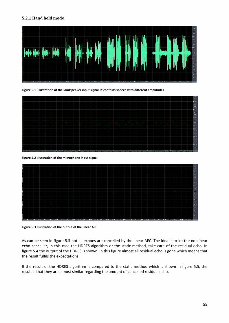
59

5.2.1 Hand held mode

Figure 5.1 Illustration of the loudspeaker input signal. It contains speech with different amplitudes

Figure 5.2 Illustration of the microphone input signal

Figure 5.3 Illustration of the output of the linear AEC

As can be seen in figure 5.3 not all echoes are cancelled by the linear AEC. The idea is to let the nonlinear echo canceller, in this case the HDRES algorithm or the static method, take care of the residual echo. In figure 5.4 the output of the HDRES is shown. In this figure almost all residual echo is gone which means that the result fulfils the expectations. If the result of the HDRES algorithm is compared to the static method which is shown in figure 5.5, the result is that they are almost similar regarding the amount of cancelled residual echo.

60

Figure 5.4 Illustration of the output of the HDRES algorithm

Figure 5.5 Illustration of the output of the static method output

To have a better look at the result a magnified view of the output of the linear AEC, the HDRES and the static method is shown in figures 5.6, 5.7 and 5.8 respectively. In this comparison it is clearer how much of the residual echo from the linear AEC is reduced. It is also visible that the static method has a better performance in cancelling residual echo than the HDRES.

Figure 5.6 Illustration of the output of the linear AEC magnified

61

Figure 5.7 Illustration of the output of the HDRES output magnified

Figure 5.8 Illustration of the output of the static output magnified

5.2.2 Hands free mode case For the hands free mode the same comparison as for the hand held mode is made. The loudspeaker input, microphone input, AEC output, HDRES output and the Static method output are illustrated in figures 5.9, 5.10, 5.11, 5.12 and 5.13 respectively.

Figure 5.9 Illustration of the loudspeaker input signal. It contains speech with different amplitudes

62

Figure 5.10 Illustration of the microphone input signal


Figure 5.12 Illustration of the output of HDRES

Figure 5.13 Illustration of the static output

63

The results from the hands free mode are similar to the results for the hand held mode. Thus, almost all the residual echo is cancelled. The comparison between the output from the HDRES model and the static method gives a similar result. If the plots for the HDRES output and the static model output are magnified the result will be like in figure 5.14 and figure 5.15. In this comparison it is more clear that the static model gives a better result in cancelling the residual echo, although the difference is small.

Figure 5.14 Illustration of the HDRES output magnified

Figure 5.15 Illustration of the static output magnified

5.2.3 Results for the double talk situation For this comparison a signal which contains double talk is considered. Thus, there are both acoustic echo from the loudspeaker and near-end speech present at the same time. In figure 5.16 the output from the linear AEC is illustrated. It is containing the mostly near-end speech but also some residual echo. The purpose of the residual echo canceller is to take care of the residual echo without cancelling the near-end speech. As mentioned earlier, adaptive methods are sensitive for double talk, and so is the HDRES algorithm. This is quite clear if the red marked areas in the plots are compared to each other. The area is containing near-end speech mixed with residual echo which gives the result that the HDRES simply takes away everything, as illustrated in figure 5.17. The static method, which is illustrated in figure 5.18, has a better performance in this case.

64


Figure 5.17 Illustration of the output of the HDRES

Figure 5.18 Illustration of the output of the static method

65

Performance measurement:

The most common method to measure performance of acoustic echo canceller is Echo Return Loss Enhancement (ERLE). ERLE shows how much of the echo captured by the microphone is cancelled by the acoustic echo canceller in dB scale. It is defined as the ratio of residual echo power to echo power at the microphone [11].

(/´( $ %=�97< �&Ã+fh,Ã+0h,&�

where � and � are residual echo and microphone input signals respectively. A good AEC is expected to have a high value of ERLE. ERLE is used only for single talk scenarios. Since this thesis focuses on nonlinear acoustic echo cancellers, measuring their performance irrespectively of the linear AEC used before them is possible if the ERLE is modified to Nonlinear Echo Return Loss Enhancement (NERLE) defined as the ratio between power of the output from nonlinear echo canceller and power of the residual echo (output of the linear AEC). Hence the following NERLE definition is used to measure the performances of the HDRES algorithm and static method [11]:

Â(/´( $ %=�97<Ú&(+8�,(+��,&Û

where 8 is output of the nonlinear echo canceller and � is the residual echo. Hands free Mode

Performances of the HDRES algorithm and the static method when measured by NERLE are shown in Figures 5.19 and 5.20 respectively. Both methods have high NERLE values showing their nonlinear echo cancelling performance [11].

Figure 5.19 NERLE of HDRES algorithm in Hands free mode (single talk)

66

Figure 5.20 NERLE of Static method in hands free mode (single talk)

Hand held Mode

Figures 5.21 and 5.22 show NERLE measurement of the HDRES and the static method respectively. The two algorithms have higher NERLE values in hands free mode than in hand held mode which implies that they perform well for hands free mode. This is because nonlinear echo is more prominent in hands free mode than in hand held mode [11].

Figure 5.21 NERLE of HDRES algorithm in hand held mode (single talk)

67

Figure 5.22 NERLE of the static method in hand held mode (single talk)

68

CHAPTER 6 CONCLUSION AND FURTHER WORK

69

6.1 Conclusion This thesis is considering the fact that an adaptive method is needed to cancel residual nonlinear echo. The question that was asked in the problem statement was:

• Is there any adaptive method to cancel nonlinear acoustic echo in a way that is suitable for mobile phones?

To answer this question an adaptive algorithm named HDRES, short for Harmonic Distortion Residual Echo Suppression been implemented in an operating acoustic echo cancelling system and has been tested. The project was initiated by a number of measurements being performed on three different mobile phones that were documented to have problems with nonlinear acoustic echo. The measurements were analysed to characterize the problem of nonlinearities produced by mobile phone loudspeakers. When the problem was identified an investigation was started in order to look for already published articles that were discussing nonlinear acoustic echo cancellation. From this wide field of different concepts three articles were chosen for a closer investigation. From those articles one method was chosen to become implemented and tested. The result of the implementation of the chosen method was an algorithm that showed good performance in cancelling nonlinear echo. The simulation testing that was done showed that almost all residual echoes were cancelled. However, the sensitivity to doubletalk of the method that was stated in the article was shown to be correct. At some parts of the signal where doubletalk was presented, the near-end speech was reduced or even completely erased. Some attempts were made to minimize the sensitivity of the doubletalk, e.g. weight limitation, but with no results. When the HDRES is compared to the static nonlinear canceller, it can be said that the HDRES has a similar performance to the static method in cancelling nonlinear echo. However, the performance in handling doubletalk was significantly better for the static method. To answer the question, it might be possible to use an operating adaptive algorithm to cancel the nonlinear echo in an AEC system, which has both low computational compexity and fast convergence. However, the prerequisite for such a system to work would be that a doubletalk detector is implemented along with the adaptive algorithm. That way the doubletalk situation could be found and the adaptation of the algorithm could be stopped. Thus, the major part of the speech would be saved.

70

6.2 Further work The problem of echo in general and nonlinear echo in particular is significant in the ever-increasing development of hands free communication devices. As the trend in the technology is to make everything wireless and portable, it is evident that this problem will get worse in the future due to cheap loudspeakers. In this thesis, ways of cancelling nonlinear echo are presented. Moreover the selected algorithm for implementation has cancelled most of the nonlinear echo. But further improvements can be done to handle the following:

• Double talk

• Other types of non linear distortion such as spectral leakage in addition to harmonic distortion. • Minimization of near-end speech distortion

Finally the complexity of the algorithm is not tested by running it on a cell phone, which should be done before heading to use it on real applications.

71

References [[1] Jacob B., Yiteng H., Adaptive signal processing: applications to real-world problems, 2003, Springer, Berlin. [2] Stran G. & Nguyen T., Wavelets and Filter Banks, 1996, Wellesley-Cambridge Press, Wellesley. [3] Saeed V., Advanced Digital Signal Processing and Noise Reduction, 3rd edition, 2006, John Wiley and Sons Ltd.

[4] Manson H., Statisticla Digital Signal Processing and Modelling, 1996, John Wiley and sons inc [5] Nordebo S., “Signal Processing Antennas II”, Lecture notes, 2004 [6] Ogunfunmi T., Adaptive Nonlinear System Idenfication: The volterra and Wiener model approaches, 2007, Springer New York

[7] Ballou, G., Handbook for sound engineers, 2002, Elsevier inc. Oxford UK.

[8] Klippel, W. “Loudspeaker Nonlinearities – Causes, Parameters, Symptoms” Dresten, Germany

[9] Kuech, F. & Kellerman, W., “Nonlinear residual echo suppression using a power filter model of the acoustic echo path”, 2007, ICASSP

[10] Everest, F. A., Master Handbook of Acoustics, McGraw-Hill Professional Publishing, 2000, USA, Ohio.

[11] ÅHGREN P., On system Identification and Acoustic Echo Cancellation, 2004, Phd Thesis Uppsala University. [12] Ljung, L., System Identification: Theory For the User, 2nd ed, 1999, PTR 92HPrentice Hall, Upper Saddle River, New Jersey.

[13] Deepa S., Tessamma T., “Nonlinear Modeling of Loudspeaker Using Adaptive Second Order Filters”, 2007, ICTES [14] Hänsler E., Schmidt G., Acoustic Echo and Noise Control: A Practical Approach, 2005, John Wiley & Sons, USA. [15] Toumazou C., Circuits and Systems tutorials, 1996, IEEE Press [16] Zaknich A., HPrinciples of Adaptive Filters and Self-learning Systems, 2005, Springer

[17] Azpicueta-Ruiz L. A., Zeller M., Arenas-Garcia J., and Kellermann W., “Novel Schemes for Nonlinear Acoustic echo cancellation based on filter combinations”, 2009, IEEE, ICASSP. [18] Arenas-Garc´ıa J., Figueiras-Vidal A. R. and A. H. Sayed, “Mean-square performance of a convex combination of two adaptive filters,” 2006, IEEE Trans. Signal Process., vol. 54, pp. 1078–1090.

[19] Umoh, I. J. and Ogunfunmi, T., “An Adaptive Nonlinear Filter for System Identification”, 2009, EURASIP Journal on Advances in Signal Processing Vol. 2009, pp 1-7 [20] Kun S., Xiaoli Ma, G.Tong Z., “An efficient acoustic echo cancellation design for systems with long room impulses and nonlinear loudspeakers”, 2008, Signal Processing. An International Journal No. 89, pp 121-132 [21] Melsa Peter J. W, Younce R. C. and Robs C. E., “Impulsive Response Shortening for Discrete Multitone Transceivers”, 1996, IEEE Transactions on Communications, Vol. 44, No. 12

http://en.wikipedia.org/wiki/Lennart_Ljung

http://en.wikipedia.org/wiki/Prentice_Hall

http://www.springerlink.com/content/h10544/?p=327bad2bfdff4500be8168b8936b59f8&pi=0

72

[22] Bendersky, Diego A., Stokes, J. W. and Malvar, Henrique S., “Nonlinear residual acoustic echo suppression for high levels of harmonic distortion”, 2008 IEEE International Conference on Acoustics, Speech and Signal Processing [23] Hansler, E. E., Acoustic echo and noise control: a practical approach, 2004, John Wiley & Sons, Inc., Hoboken, New Jersey. [24] Malvar, H.S., “A modulated complex lapped transform and its applications to audio processing”, 1999, ICASSP.

73

Appendix A Matlab Code The Matlab code of the Harmonic Distortion Residual Echo Suppression algorithm. %############################## Initialization ############################ MIN_GAIN = 0.01; %Minimum Gain allowed fs = 8000; %sample rate N = 256; %N point FFT size M = 16; %Number of frequency bands for 8kHz sampling frequency H = 6; %Number of harmonics including fundamentalband mapping L = 0; %Echo leakage window(Denoted by K on the paper) mu = 0.07; %step size beta = 1; %tunes agressiveness of the Gk(m) algorithm alpha = 0.5; %controls amount of smoothing rho = 0.25; %power estimate smoothing Sk = zeros(1,M); %Speech in the near end Nk = zeros(1,M); %Noise in the near end Nks = zeros(2,M); %Noise(two rows needed to store the current and

previous noise) Drk = zeros(1,M); %Reference residual echo signal Drks = zeros(2,M); %Smoothed estimation of residual echo signal Ek = zeros(1,M); %Output of the linear AEC Eks = zeros(2,M)+ eps; %Smoothed update of output of the linear AEC Xk = zeros(1,M); %frequency banded input signal in frequency domain Pk = zeros(2,M)+eps; %Average power of speaker input signal WR = zeros(M,M,H,2*L+1); %Weight for Residual echo estimation ThresholdPowerRxdBovl = -30; ThresholdPowerRx = 10^(ThresholdPowerRxdBovl/10)*(32768)^2*N*N*8/2; Blocksize = 80; MaxValue = 0; WeightLimit = 0.15; %Initialization: Input signals f = 536; %fundamental frequency num_harmonics = 6; %number of harmonics w0 = 2*pi*f/fs; n = (0:10000); fvec = (0:128-1)*8000/256; dr = 0; %dr starts with the value 0 A_org = 1*(2^(15)-1); % = 32767 min_value1 = 0.5; %min random value 1 max_value1 = 1; %max random value 1 min_value2 = 0; %min random value 2 max_value2 = 0.5; %max random value 2 ref=(1:128)*8000/256; %Initialization: Estimated resudual echo temp = 0; %############# CHECK FOR HARMONICS LIMIT ################################## if (f*num_harmonics > fs/2) error('To many harmonics considered'); end %############# CREATE THE INPUT SIGNAL ################################### x = A_org*sin(w0*n); %Loudspeaker input signal for j = 1:num_harmonics %dr=SUM[A*sin(w0*n+P)](summation of sinusiodal)

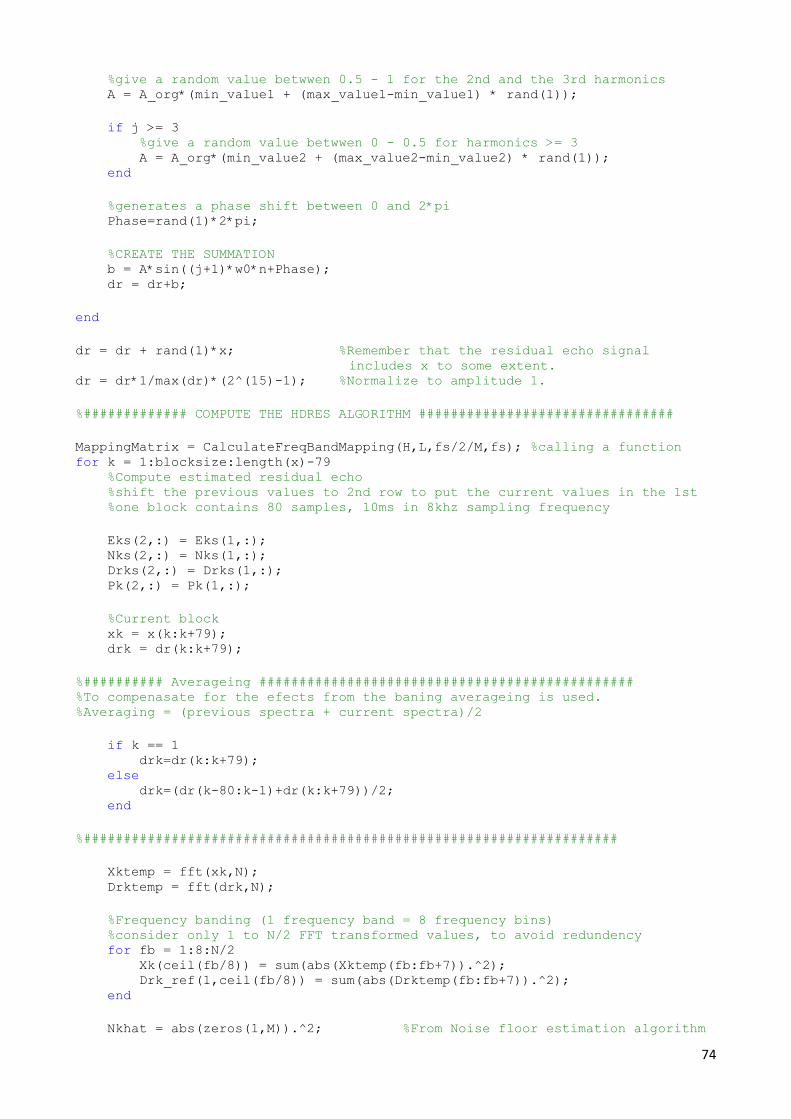
74

%give a random value betwwen 0.5 - 1 for the 2nd and the 3rd harmonics A = A_org*(min_value1 + (max_value1-min_value1) * rand(1)); if j >= 3 %give a random value betwwen 0 - 0.5 for harmonics >= 3 A = A_org*(min_value2 + (max_value2-min_value2) * rand(1)); end %generates a phase shift between 0 and 2*pi Phase=rand(1)*2*pi; %CREATE THE SUMMATION b = A*sin((j+1)*w0*n+Phase); dr = dr+b; end dr = dr + rand(1)*x; %Remember that the residual echo signal

includes x to some extent. dr = dr*1/max(dr)*(2^(15)-1); %Normalize to amplitude 1. %############# COMPUTE THE HDRES ALGORITHM ################################ MappingMatrix = CalculateFreqBandMapping(H,L,fs/2/M,fs); %calling a function for k = 1:blocksize:length(x)-79 %Compute estimated residual echo %shift the previous values to 2nd row to put the current values in the 1st %one block contains 80 samples, 10ms in 8khz sampling frequency Eks(2,:) = Eks(1,:); Nks(2,:) = Nks(1,:); Drks(2,:) = Drks(1,:); Pk(2,:) = Pk(1,:); %Current block xk = x(k:k+79); drk = dr(k:k+79); %########## Averageing ############################################### %To compenasate for the efects from the baning averageing is used. %Averaging = (previous spectra + current spectra)/2 if k == 1 drk=dr(k:k+79); else drk=(dr(k-80:k-1)+dr(k:k+79))/2; end %################################################################### Xktemp = fft(xk,N); Drktemp = fft(drk,N); %Frequency banding (1 frequency band = 8 frequency bins) %consider only 1 to N/2 FFT transformed values, to avoid redundency for fb = 1:8:N/2 Xk(ceil(fb/8)) = sum(abs(Xktemp(fb:fb+7)).^2); Drk_ref(1,ceil(fb/8)) = sum(abs(Drktemp(fb:fb+7)).^2); end Nkhat = abs(zeros(1,M)).^2; %From Noise floor estimation algorithm

75

Ek = Nk + Sk + Drk_ref; Xprimek = Xk; %No delay in this case for mm = 1:length(Xprimek) if (Xprimek(mm) < ThresholdPowerRx) %Prevent bands not powerful

enough to contribute to Harmonics Xprimek_masked(mm) = 0; else Xprimek_masked(mm) = Xprimek(mm); end end %POWER SMOOTHING for m = 1:M Pk(1,m) = (1-rho)*Pk(2,m) + rho*((Xprimek(m))^2); if(Pk(1,m)< Minimum_power) Pk(1,m) = Minimum_power; end end for m = 1:M %FREQUENCY BAND temp = 0; %Initialization for each f-band for i = 1:m %fundamental frequency band for j = 1:H %number of harmonics for l = -L:L %echo leakage if (MappingMatrix(m,i,j,l+(L+1)) == 1) temp = temp + WR(m,i,j,l+(L+1))*Xprimek_masked(i); end end end end Drhatk(m) = temp; %Estimated Residual Echo if (Drhatk(m) < 0), Drks(1,m)= (1-alpha)*Drks(2,m); else Drks(1,m)= (1-alpha)*Drks(2,m) + alpha*(Drhatk(m)); end %smoothing %second row in Ek, Drk, Nk, Pk refers to the prevous signal Eks(1,m) = (1-alpha)*Eks(2,m) + alpha*(Ek(m)); Nks(1,m) = (1-alpha)*Nks(2,m) + alpha*(Nkhat(m)); %Gain computation Gk(m) = max(max(Eks(1,m)-

beta*Drks(1,m),Nks(1,m))/abs(Eks(1,m)),MIN_GAIN); %error computation for adaptation of WR errk(m) = Ek(m) - Drhatk(m); for i=1:m if (Xprimek_masked(i) > 0) for j=1:H if (MappingMatrix(m,i,j == 1) WR(m,i,j) = WR(m,i,j) +(mu/Pk(1,i))*Xprimek(i)*errk(m); if WR(m,i,j) > WeightLimit WR(m,i,j)= WeightLimit; end end end end end end end %End for each frequency band

76

end %End for each frame The Matlab code of the mapping matrix function [MappingMatrix] = CalculateFreqBandMapping(NbrHarmonics,WindowLength,Bandwidth,SampleRate) % Calculate the mapping of contributing frequency band. SampleRateBy2 = SampleRate/2; NbrFreqBands = SampleRateBy2/Bandwidth; FreqLowLimit = Bandwidth*(0:1:NbrFreqBands-1); FreqLowLimit(1) = 30; %Approximative lowest frequency of usage- DEPEND ON FFT

RESOLUTION (2 bin) FreqHighLimit = Bandwidth*(1:1:NbrFreqBands)-1; %l = 0 - No leakage or search window applied for i = 1:NbrFreqBands, for j = 1:NbrHarmonics; LowestBand = floor(FreqLowLimit(i)*j/Bandwidth); HighestBand = floor(FreqHighLimit(i)*j/Bandwidth); BandNumberIndex = (LowestBand:1:HighestBand)+1; BandNumberIndex = BandNumberIndex(find(BandNumberIndex <= NbrFreqBands)); BandNumberIndex = BandNumberIndex(find(BandNumberIndex >= 1)); MappingMatrix(BandNumberIndex,i,j) = 1; end end

Appendix B Measurement plots

Frequency sweep

White noise

Loudspeaker input. Frequency sweep with a high amplitude, frequency domain

Microphone input. Frequency sweep with a high amplitude, frequency domain

Loudspeaker input. Frequency sweep with a low amplitude, frequency domain.

Microphone input. Frequency sweep with a low amplitude, frequency domain.

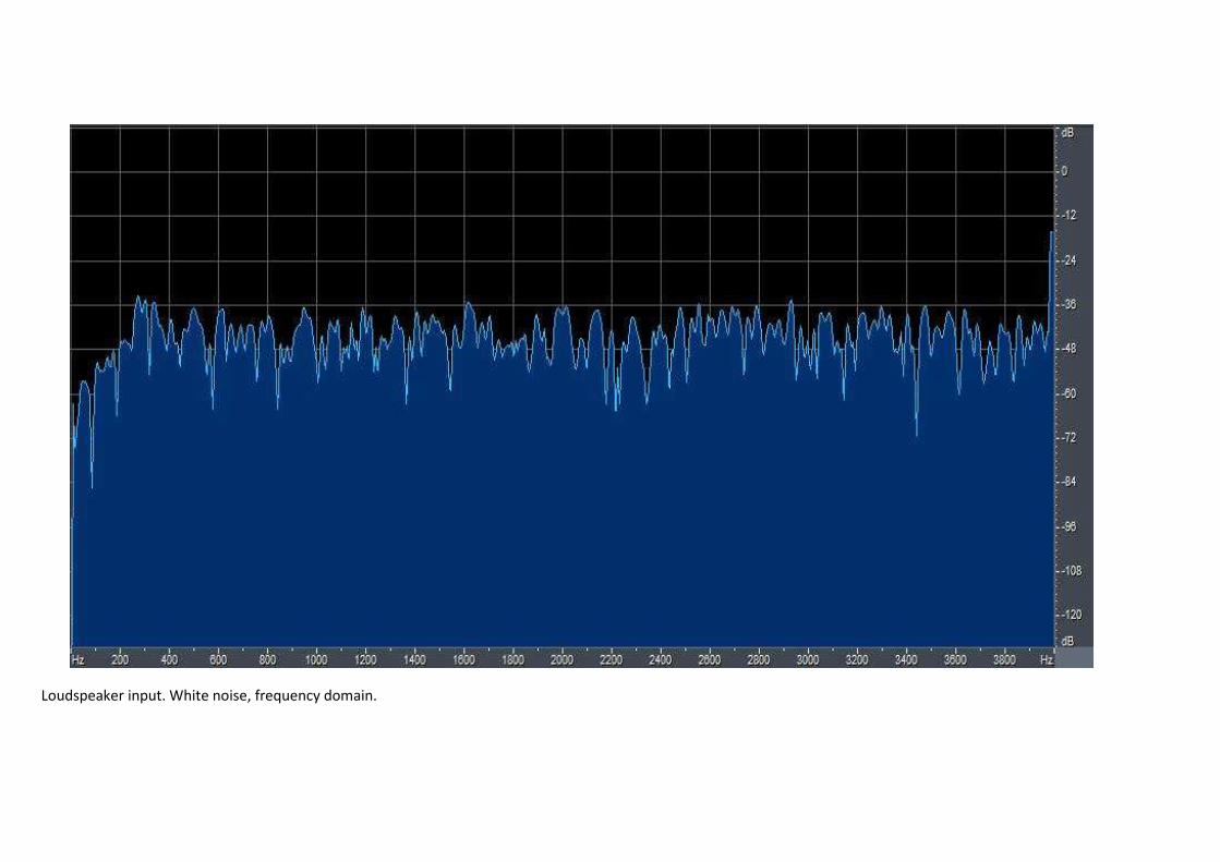
Loudspeaker input. White noise, frequency domain.

Microphone input. White noise, frequency domain

Loudspeaker input. Frequency sweep with a high amplitude, frequency domain

Microphone input. Frequency sweep with a high amplitude, frequency domain

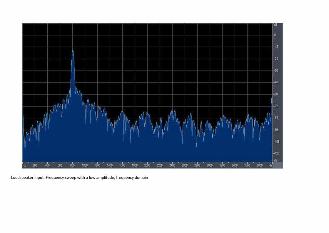
Loudspeaker input. Frequency sweep with a low amplitude, frequency domain

Microphone input. Frequency sweep with a low amplitude, frequency domain

Measured with an external microphone. Loudspeaker input, frequency sweep, frequency domain

Measured with an external microphone. Microphone input, frequency sweep, frequency domain

Appendix C Result plots

Illustration of the loudspeaker input signal. It contains speech with different amplitudes

Illustration of the output of the linear AEC magnified

Illustration of the output of the HDRES output magnified

llustration of the output of the static output magnified

Illustration of the loudspeaker input signal. It contains speech with different amplitudes

Illustration of the microphone input signal

Illustration of the output of the linear AEC

I llustration of the HDRES output magnified

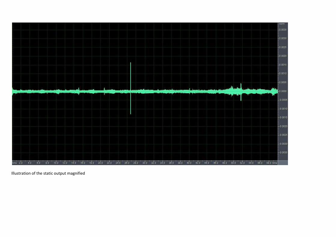
Illustration of the static output magnified

Illustration of the output of the linear AEC

I llustration of the output of the HDRES

Illustration of the output of the static method

SE-351 95 Växjö / SETel [email protected]

351 95 Växjö / SE-391 82 Kalmar 772-28 80 00

[email protected]

Documents

Nonlinear Acoustic Echo Cancellation for Mobile Phones: A ...lnu.diva-portal.org/smash/get/diva2:323399/FULLTEXT01.pdf · The result of this thesis has shown that it might be possible