Non-Restoring Integer Square Root:A Case Study in Design by Principled

Optimization

John O'Leary1, Miriam Leeser1 , Jason Hickey2, Mark Aagaard1

1 School Of Electrical EngineeringCornell UniversityIthaca, NY 14853

2 Department of Computer ScienceCornell UniversityIthaca, NY 14853

Abstract. Theorem proving techniques are particularly well suited forreasoning about arithmetic above the bit level and for relating di�erentlevels of abstraction. In this paper we show how a non-restoring integersquare root algorithm can be transformed to a very e�cient hardwareimplementation. The top level is a Standard ML function that operateson unbounded integers. The bottom level is a structural description ofthe hardware consisting of an adder/subtracter, simple combinationallogic and some registers. Looking at the hardware, it is not at all obviouswhat function the circuit implements. At the top level, we prove that thealgorithm correctly implements the square root function. We then showa series of optimizing transformations that re�ne the top level algorithminto the hardware implementation. Each transformation can be veri�ed,and in places the transformations are motivated by knowledge about theoperands that we can guarantee through veri�cation. By decomposingthe veri�cation e�ort into these transformations, we can show that thehardware design implements a square root. We have implemented thealgorithm in hardware both as an Altera programmable device and infull-custom CMOS.

1 Introduction

In this paper we describe the design, implementation and veri�cation of a sub-tractive, non-restoring integer square root algorithm. The top level description isa Standard ML function that implements the algorithm for unbounded integers.The bottom level is a highly optimized structural description of the hardwareimplementation. Due to the optimizations that have been applied, it is very dif-�cult to directly relate the circuit to the algorithmic description and to provethat the hardware implements the function correctly. We show how the proofcan be done by a series of transformations from the SML code to the optimizedstructural description.

At the top level, we have used the Nuprl proof development system [Lee92]to verify that the SML function correctly produces the square root of the input.

We then use Nuprl to verify that transformations to the implementation preservethe correctness of the initial algorithm.

Intermediate levels use Hardware ML [OLLA93], a hardware description lan-guage based on Standard ML. Starting from a straightforward translation ofthe SML function into HML, a series of transformations are applied to obtainthe hardware implementation. Some of these transformations are expressly con-cerned with optimization and rely on knowledge of the algorithm; these trans-formations can be justi�ed by proving properties of the top-level description.

The hardware implementation is highly optimized: the core of the design is asingle adder/subtracter. The rest of the datapath is registers, shift registers andcombinational logic. The square root of a 2n bit wide number requires n cyclesthrough the datapath. We have two implementations of square root chips basedon this algorithm. The �rst is done as a full-custom CMOS implementation; thesecond uses Altera EPLD technology. Both are based on a design previouslypublished by Bannur and Varma [BV85]. Implementing and verifying the designfrom the paper required clearing up a number of errors in the paper and clarifyingmany details.

This is a good case study for theorem proving techniques. At the top level,we reason about arithmetic operations on unbounded integers, a task theoremprovers are especially well suited for. Relating this to lower levels is easy todo using theorem proving based techniques. Many of the optimizations used areapplicable only if very speci�c conditions are satis�ed by the operands. Verifyingthat the conditions hold allows us to safely apply optimizations.

Automated techniques such as those based on BDDs and model checking arenot well-suited for verifying this and similar arithmetic circuits. It is di�cultto come up with a Boolean statement for the correctness of the outputs as afunction of the inputs and to argue that this speci�cation correctly describesthe intended behavior of the design. Similarly, speci�cations required for modelcheckers are di�cult to de�ne for arithmetic circuits.

There have been several veri�cations of hardware designs which lift the rea-soning about hardware to the level of integers, including the Sobel Image pro-cessing chip [NS88], and the factorial function [CGM86]. Our work di�ers fromthese and similar e�orts in that we justify the optimizations done in order torealize the square root design. The DDD system [BJP93] is based on the idea ofdesign by veri�ed transformation, and was used to derive an implementation ofthe FM9001 microprocessor. High level transformations in DDD are not veri�edby explicit use of theorem proving techniques.

The most similar research is Verkest's proof of a non-restoring division algo-rithm [VCH94]. This proof was also done by transforming a design descriptionto an implementation. The top level of the division proof involves considerationof several cases, while our top level proof is done with a single loop invariant.The two implementations vary as well: the division algorithm was implementedon an ALU, and the square root on custom hardware. The algorithms and im-plementations are su�ciently similar that it would be interesting to develop asingle veri�ed implementation that performs both divide and square root based

on the research in these two papers.The remainder of this paper is organized as follows. In section 2 we describe

the top-level non-restoring square root algorithm and its veri�cation in the Nuprlproof development system. We then transform this algorithm down to a levelsuitable for modelling with a hardware description language. Section 3 presentsa series of �ve optimizing transformations that re�ne the register transfer leveldescription of the algorithm to the �nal hardware implementation. In section 4we summarize the lessons learned and our plans for future research.

2 The Non-Restoring Square Root Algorithm

An integer square root calculates y =px where x is the radicand, y is the root,

and both x and y are integers. We de�ne the precise square root (p) to be thereal valued square root and the correct integer square root to be the oor of theprecise root. We can write the speci�cation for the integer square root as shownin De�nition 1.

De�nition 1 Correct integer square root

y is the correct integer square root of x =̂ y2 � x < (y + 1)2

We have implemented a subtractive, non-restoring integer square root algo-rithm [BV85]. For radicands in the range x = f0::22n� 1g, subtractive methodsbegin with an initial guess of y = 2(n�1) and then iterate from i = (n � 1) : : :0.In each iteration we square the partial root (y), subtract the squared partial rootfrom the radicand and revise the partial root based on the sign of the result.There are two major classes of algorithms: restoring and non-restoring [Flo63].In restoring algorithms, we begin with a partial root for y = 0 and at the end ofeach iteration, y is never greater than the precise root (p). Within each iteration(i), we set the ith bit of y, and test if x� y2 is negative; if it is, then setting theith bit made y too big, so we reset the ith bit and proceed to the next iteration.

Non-restoring algorithms modify each bit position once rather than twice.Instead of setting the the ith bit of y, testing if x�y2 is positive, and then possiblyresetting the bit; the non-restoring algorithms add or subtract a 1 in the ith bitof y based on the sign of x� y2 in the previous iteration. For binary arithmetic,the restoring algorithm is e�cient to implement. However, most square roothardware implementations use a higher radix, non-restoring implementation. Forhigher radix implementations, non-restoring algorithms result in more e�cienthardware implementations.

The results of the non-restoring algorithms do not satisfy our de�nition ofcorrect, while restoring algorithms do satisfy our de�nition. The resulting valueof y in the non-restoring algorithms may have an error in the last bit position.For the algorithm used here, we can show that the �nal value of y will always beeither the precise root (for radicands which are perfect squares) or will be oddand be within one of the correct root. The error in non-restoring algorithms iseasily be corrected in a cleanup phase following the algorithm.

Below we show how a binary, non-restoring algorithm runs on some valuesfor n =3. Note that the result is either exact or odd.

x = 1810 = 101002 iterate 1 y = 100 x� y2 = +iterate 2 y = 110 x� y2 = �iterate 3 y = 101

x = 1510 = 011112 iterate 1 y = 100 x� y2 = �iterate 2 y = 010 x� y2 = +iterate 3 y = 011

x = 1610 = 100002 iterate 1 y = 100 x� y2 = 0

In our description of the non-restoring square root algorithm, we de�ne adatatype state that contains the state variables. The algorithm works by ini-tializing the state using the function init, then updating the state on eachiteration of the loop by calling the function update. We re�ne our programthrough several sets of transformations. At each level the de�nition of state,init and update may change. The SML code that calls the square root at eachlevel is:

fun sqrt n radicand = iterate update (n-1) (init n radicand)

The iterate function performs iteration by applying the function argumentto the state argument, decrementing the count, and repeating until the count iszero.

fun iterate f n state =

if n = 0 then state else iterate f (n - 1) (f state)

The top level (L0) is a straightforward implementation of the non-restoringsquare root algorithm. We represent the state of an iteration by the tripleStatefx,y,ig where x is the radicand, y is the partial root, and i is the it-

eration number. Our initial guess is y = 2(n�1). In update, x never changes andi is decremented from n-2 to 1, since the initial values take care of the (n� 1)st

iteration. At L0, init and update are:

fun init (n,radicand) =

State{x = radicand, y = 2 ** (n-1), i = n-2 }

fun update (State{x, y, i}) =

let

val diffx = x - (y**2)

val y' = if diffx = 0 then y

else if diffx > 0 then (y + (2**i))

else (* diffx < 0 *) (y - (2**i))

in

State{x = x, y = y', i = i-1 }

end

In the next section we discuss the proof that this algorithm calculates thesquare root. Then we show how it can be re�ned to an implementation thatrequires signi�cantly less hardware. We show how to prove that the re�ned al-gorithm also calculates the square root; in the absence of such a proof it is notat all obvious that the algorithms have identical results.

2.1 Veri�cation of Level Zero Algorithm

All of the theorems in this section were veri�ed using the Nuprl proof develop-ment system. Theorem 1 is the overall correctness theorem for the non-restoringsquare root code shown above. It states that after iterating through update forn-1 times, the value of y is within one of the correct root of the radicand. Wehave proved this theorem by creating an invariant property and performing in-duction on the number of iterations of update. Remember that n is the numberof bits in the result.

Theorem 1 Correctness theorem for non-restoring square root algorithm

` 8n : 8radicand : f0::22n� 1g :let

Statefx; y; ig = iterate update (n � 1) (init n radicand)in

(y � 1)2 � radicand < (y + 1)2

end

The invariant states that in each iteration y increases in precision by 2i, andthe lower bits in y are always zero. The formal statement (I) of the invariant isshown in De�nition 2.

De�nition 2 Loop invariant

I(Statefx; y; ig) =̂((y � 2i)2 � radicand < (y + 2i)2) & (y rem 2i = 0) & (x = radicand)

In Theorems 2 and 3 we show that init and update are correct, in that for alllegal values of n and radicand, init returns a legal state and for all legal inputstates, update will return a legal state and makes progress toward terminationby decrementing i by 1. A legal state is one for which the loop invariant holds.

Theorem 2 Correctness of initialization

` 8n : 8radicand : f0::22n� 1g:8x; y; i :Statefx; y; ig = init n radicand =)I(Statefx; y; ig) & (x = radicand) & (y = 2n�1) & (i = n � 2)

Theorem 3 Correctness of update

` 8x; y; i : I((Statefx; y; ig)) =)8x0; y0; i0 : Statefx0; y0; i0g = update (Statefx; y; ig) =)I(Statefx0; y0; i0g) & (i0 = i � 1)

The correctness of init is straightforward. The proof of Theorem 3 relies onTheorem 4, which describes the behavior of the update function. The body ofupdate has three branches, so the proof of correctness of update has three parts,depending on whether x� y2 is equal to zero, positive, or negative. Each casein Theorem 4 is straightforward to prove using ordinary arithmetic.

Theorem 4 Update lemmas

Case x� y2 = 0` 8x; y; i : I((Statefx; y; ig)) =)

(x � y2 = 0) =) I(Statefx; y; i� 1g)

Case x� y2 > 0` 8x; y; i : I((Statefx; y; ig)) =)

(x � y2 > 0) =) I(Statefx; y + 2i; i� 1g)

Case x+ y2 > 0` 8x; y; i : I((Statefx; y; ig)) =)

(x + y2 > 0) =) I(Statefx; y � 2i; i� 1g)

We now prove that iterating update a total of n-1 times will produce thecorrect �nal result. The proof is done by induction on n and makes use of Theo-rem 5 to describe one call to iterate. This allows us to prove that after iteratingupdate a total of n-1 times, our invariant holds and i is zero. This is su�cientto prove that square root is within one of the correct root.

Theorem 5 Iterating a function

` 8prop; n; f; s:prop n s =)

(8n0; s0:prop n0 s0 =) prop (n0 � 1) (f s0)) =)prop 0 (iterate f n s)

2.2 Description of Level One Algorithm

The L0 SML code would be very expensive to directly implement in hardware.If the state were stored in three registers, x would be stored but would neverchange; the variable i would need to be decremented every loop and we wouldneed to calculate y2, x� y2, 2i, and y� 2i in every iteration. All of these areexpensive operations to implement in hardware. By restructuring the algorithm

through a series of transformations, we preserve the correctness of our designand generate an implementation that uses very little hardware.

The key operations in each iteration are to compute x� y2 and then update yusing the new value y0 = y� 2i, where � is + if x � y2 � 0 and � if x� y2 < 0.The variable x is only used in the computation of x� y2. In the L1 code weintroduce the variable diffx, which stores the result of computing x� y2. Thishas the advantage that we can incrementally update diffx based on its valuein the previous iteration:

y' = y� 2i

y02 = y2 � 2 � y � 2i + (2i)2

= y2 � y � 2i+1 + 22�i

diffx = x� y2

diffx'= x� y02

= x� (y2 � y � 2i+1 + 22�i)

= (x� y2) � y � 2i+1 � 22�i

The variable i is only used in the computations of 22�i and y � 2i+1, so wecreate a variable b that stores the value 22�i and a variable yshift that storesy � 2i+1. We update b as: b' = b div 4. This results in the following equationsto update yshift and diffx:

y0 � 2i+1 = (y� 2i) � 2i+1yshift0 = y � 2i+1 � 2i � 2i+1

= yshift� 2 � 22�i= yshift� 2 � b

diffx0 = diffx� yshift� b

The transformations from L0 to L1 can be summarized:

diffx = x� y2 yshift = y � 2i+1 b = 22�i

The L1 versions of init and update are given below. Note that, although theoptimizations are motivated by the fact that we are doing bit vector arithmetic,the algorithm is correct for unbounded integers. Also note that the most complexoperations in the update loop are an addition and subtraction and only oneof these two operations is executed each iteration. We have optimized away allexponentiation and any multiplication that cannot be implemented as a constantshift.

fun init1 (n,radicand) =

let

val b' = 2 ** (2*(n-1))

in

State{diffx = radicand - b',

yshift = b',

b = b' div 4

}

end

fun update1 (State{diffx, yshift, b}) =

let

val (diffx',yshift') =

if diffx > 0 then (diffx - yshift - b, yshift + 2*b)

else if diffx = 0 then (diffx , yshift )

else (* diffx < 0 *) (diffx + yshift - b, yshift - 2*b)

in

State{diffx = diffx',

yshift = yshift' div 2,

b = b div 4

}

endWe could verify the L1 algorithm from scratch, but since it is a transformation

of the L0 algorithm, we use the results from the earlier veri�cation. We do thisby de�ning a mapping function between the state variables in the two levels andthen proving that the two levels return equal values for equal input states. Thetransformation is expressed as follows:

De�nition 3 State transformation

T (Statefx; y; ig; Statefdi�x ; yshift; bg) =̂(di�x = x� y2 & yshift = y � 2i+1 & b = 22�i)

All of the theorems in this section were proved with Nuprl. In Theorem 6 wesay that for equal inputs init1 returns an equivalent state to init. In Theorem 7we say that for equivalent input states, update1 and update return equivalentoutputs.

Theorem 6 Correctness of initialization

` 8n : 8radicand : f0::22n� 1g:8x; y; i :Statefx; y; ig = init n radicand =)8di�x ; yshift; b :Statefdi�x ; yshift; bg = init1 n radicand =)T (Statefx; y; ig; Statefdi�x ; yshift; bg)

Theorem 7 Correctness of update

` 8x; y; i; di�x ; yshift; b :T (Statefx; y; ig; Statefdi�x ; yshift; bg) =)T (update(Statefx; y; ig); update1(Statefdi�x ; yshift; bg))

Again, the initialization theorem has an easy proof, and the update1 theoremis a case split on each of the three cases in the body of the update function,followed by ordinary arithmetic.

2.3 Description of Level Two Algorithm

To go from L1 to L2, we recognize that the operations in init1 are very similarto those in update1. By carefully choosing our initial values for diffx and y,we increase the number of iterations from n-1 to n and fold the computation ofradicand - b' in init into the �rst iteration of update. This eliminates theneed for special initialization hardware. The new initialize function is:

fun init2 (n,radicand) =

State{diffx = radicand,

yshift = 0,

b = 2 ** (2*(n-1))}

The update function is unchanged from update1. The new calling functionis:

fun sqrt n radicand = iterate update1 n (init2 n radicand)

Showing the equivalence between init2 and a loop that iterates n times andthe L1 functions requires showing that the state in L2 has the same value afterthe �rst iteration that it did after init1. More formally, init1 = update1 �init2. We prove this using the observation that, after init2, diffx is guaran-teed to be positive, so the �rst iteration of update1 in L2 always executes thediffx > 0 case. Using the state returned by init2 and performing some sim-ple algebraic manipulations, we see that after the �rst iteration in L2, update1stores the same values in the state variables as init1 did. Because both L1 andL2 use the same update function, all subsequent iterations in the L2 algorithmare identical to the L1 algorithm.

To begin the calculation of a square root, a hardware implementation ofthe L2 algorithm clears the yshift register, load the radicand into the diffx

register, and initializes the b register with a 1 in the correct location. The trans-formation from L0 to L1 simpli�ed the operations done in the loop to shifts andan addition/subtraction. Remaining transformations will further optimize thehardware.

3 Transforming Behavior to Structure with HML

The goal of this section is to produce an e�cient hardware implementation ofthe L2 algorithm. The �rst subsection introduces Hardware ML, our languagefor specifying the behavior and structure of hardware. Taking an HML versionof the L2 algorithm as our starting point, we obtain a hardware implementationthrough a sequence of transformation steps.

1. Translate the L2 algorithm into Hardware ML. Provision must be made toinitialize and detect termination, which is not required at the algorithm level.

2. Transform the HML version of L2 to a set of register assignments usingsyntactic transformations.

3. Introduce an internal state register Exact to simplify the computation, and\factor out" the condition DiffX >= %0.

4. Partition into functional blocks, again using syntactic transformations.5. Substitute lower level modules for register and combinational assignments.

Further optimizations in the implementation of the lower level modules arepossible.

Each step can be veri�ed formally. Several of these must be justi�ed by propertiesof the algorithm that we can establish through theorem proving.

3.1 Hardware ML

We have implemented extensions to Standard ML that can be used to describethe behavior of digital hardware at the register transfer level. Earlier work hasillustrated how Hardware ML can be used to describe the structure of hard-ware [OLLA93, OLLA92]. HML is based on SML and supports higher-order,polymorphic functions, allowing the concise description of regular structuressuch as arrays and trees. SML's powerful module system aids in creating param-eterized designs and component libraries.

Hardware is modelled as a set of concurrently executing behaviors commu-nicating through objects called signals. Signals have semantics appropriate forhardware modelling: whereas a Standard ML reference variable simply containsa value, a Hardware ML signal contains a list of time-value pairs representinga waveform. The current value on signal a, written $a, is computed from itswaveform and the current time.

Two kinds of signal assignment operators are supported. Combinational as-

signment, written s == v, is intended to model the behavior of combinationallogic under the assumption that gate delays are negligible. s == v causes thecurrent value of the target signal s to become v. For example, we could modelan exclusive-or gate as a behavior which assigns true to its output c wheneverthe current values on its inputs a and b are not equal:

fun Xor (a,b,c) = behavior (fn () => (c == ($a <> $b)))

HML's behavior constructor creates objects of type behavior. Its argument isa function of type unit -> unit containing HML code { in this case, a combi-national assignment.

Register assignment is intended to model the behavior of sequential circuitelements. If a register assignment s <- v is executed at time t the waveform of sis augmented with the pair (v; t+1) indicating that s is to assume the value v atthe next time step. For example, we could model a delay element as a behaviorcontaining a register assignment:

fun Reg (a,b) = behavior (fn () => (b <- $a))

Behaviors can be composed to formmore complex circuits. In the compositionof b1 and b2, written b1 || b2, both behaviors execute concurrently. We compose

our exclusive-or gate and register to build a parity circuit, which outputs falseif and only if it has received an even number of true inputs:

fun Parity (a,b) =

let

val p = signal false

in

Xor (a,b,p) || Reg (p,b)

end

RegXor

abp

The val p = : : :declaration introduces an internal signal whose initial valueis false.

Table 1 summarizes the behavioral constructs of HML. We have implementeda simple simulator which allows HML behavioral descriptions to be executedinteractively { indeed, all the descriptions in this section were developed withthe aid of the simulator.

�= signal Type of signals having values of equality type �=

signal v A signal initially having the value v$ s The current value of signal s

s == v Combinational assignments <- v Register assignment

behavior Type of behaviorsbehavior f Behavior constructorb1 || b2 Behavioral composition

Table 1. Hardware ML Constructs

3.2 Behavioral Description of the Level 2 Algorithm

It is straightforward to translate the L2 algorithm from Standard ML to Hard-ware ML. The state of the computation is maintained in the externally visiblesignal YShift and the internal signals DiffX and B. These signals correspond toyshift, diffx and b in the L2 algorithm and are capitalized to distinguish themas HML signals. For concreteness, we stipulate that we are computing an eight-bit root (n = 8 in the L2 algorithm), and so the YShift and B signals require16 bits. DiffX requires 17 bits: 16 bits to hold the initial (positive) radicandand one bit to hold the sign, which is important in the intermediate calcula-tions. We use HML's register assignment operator <- to explicitly update thestate in each computation step. The % characters preceding numeric constantsare constructors for an abstract data type num. The usual arithmetic operatorsare de�ned on this abstract type. We are thus able to simulate our descriptionusing unbounded integers, bounded integers, and bit vectors simply by providingappropriate implementations of the type and operators. The code below showsthe HML representation of the L2 algorithm. Two internal signals are de�ned,

and the behavior is packaged within a function declaration. In the future we willomit showing the function declaration and declarations of internal signals; it isunderstood that all signals except Init, XIn, YShift, and Done are internal.

val initb = %16384 (* 0x4000 *)

fun sqrt (Init, XIn, YShift, Done) =

let

(* Internal registers *)

val DiffX = signal (%0)

val B = signal (%0)

in

behavior

(fn () =>

(if $Init then

(DiffX <- $XIn;

YShift <- %0;

B <- initb;

Done <- false)

else

(if $DiffX = %0 then

(DiffX <- $DiffX;

YShift <- $YShift div %2;

B <- $B div %4)

else if $DiffX > %0 then

(DiffX <- $DiffX - $YShift - $B;

YShift <- ($YShift + %2 * $B) div %2;

B <- $B div %4)

else (* $DiffX < %0 *)

(DiffX <- $DiffX + $YShift - $B;

YShift <- ($YShift - %2 * $B) div %2;

B <- $B div %4));

Done <- $B sub 0))

end

In the SML description of the algorithm, some elements of the control stateare implicit. In particular, the initiation of the algorithm (calling sqrt) and itstermination (it returning a value) are handled by the SML interpreter. Becausehardware is free running there is no built-in notion of initiation or terminationof the algorithm. It is therefore necessary to make explicit provision to initializethe state registers at the beginning of the algorithm and to detect when thealgorithm has terminated.

Initialization is easy: the diffx, yshift, and b registers are assigned theirinitial values when the init signal is high.

In computing an eight-bit root, the L2 algorithm terminates after seven itera-tions of its loop. An e�cient way to detect termination of the hardware algorithmmakes use of some knowledge of the high level algorithm. An informal analysisof the L2 algorithm reveals that b contains a single bit, shifted right two placesin each cycle, and that the least signi�cant bit of b is set during the execution of

the last iteration. Consequently, the done signal is generated by testing whetherthe least signi�cant bit of b is set (the expression $b sub 0 selects the lsb of b)and delaying the result of the test by one cycle. done is therefore set during theclock cycle following the �nal iteration. To justify this analysis, we must formallyprove that the following is an invariant of the L2 algorithm:

(i = 1) ! (b0 = 1)

3.3 Partitioning into Register Assignments

Our second transformation step is a simple one: we transform the HML versionof the L2 algorithm into a set of register assignments. The goal of this transfor-mation is to ensure that the control state of the algorithm is made completelyexplicit in terms of HML signals.

We make use of theorems about the semantics of HML to justify transfor-mations of the behavior construct. First, if distributes over the sequentialcomposition of signal assignment statements: if P and Q are sequences of signalassignments, then

if e then

(s <- a; P)

else

(s <- b; Q)

=

if e then

s <- a

else

s <- b;

if e then P else Q

We also use a rule which allows us to push if into the right hand side of anassignment:

if e then

s <- a

else

s <- b

= s <- if e then a else b

Repeatedly applying these two rules allows us to decompose our HML codeinto a set of assignments to individual registers. The register assignments afterthis transformation are

DiffX <- (if $Init then

$XIn

else if $DiffX = %0 then

$DiffX

else if $DiffX > %0 then

$DiffX - $YShift - $B

else (* $DiffX < %0 *)

$DiffX + $YShift - $B);

YShift <- (if $Init then

%0

else if $DiffX = %0 then

$YShift div %2

else if $DiffX > %0 then

($YShift + %2 * $B) div %2

else (* $DiffX < %0 *)

($YShift - %2 * $B) div %2);

B <- (if $Init then initb else $B div %4);

Done <- (if $Init then false else $B sub 0);

3.4 Simplifying the Computation

Our third transformation step simpli�es the computation of DiffX and YShift.We begin by observing two facts about the L2 algorithm: if DiffX ever becomeszero the radicand has an exact root, and once DiffX becomes zero it remainszero for the rest of the computation. To simplify the computation of DiffX weintroduce an internal signal Exact which is set if DiffX becomes zero in thecourse of the computation.

If Exact becomes set, the value of DiffX is not used in the computationof YShift (subsequent updates of YShift involve only division by 2). DiffXbecomes a don't care, and we can merge the $DiffX = %0 and $DiffX > %0branches. We also replace $DiffX = %0with $Exact in the assignment to YShift,and change the $DiffX > %0 comparisons to $DiffX >= %0 (note that thisbranch of the if is not executed when $DiffX = %0, because Exact is set inthis case).

ExactReg <- (if $init then false else $Exact);

Exact == ($DiffX = %0 orelse $ExactReg);

DiffX <- (if $Init then

$XIn

else if $DiffX >= %0 then

$DiffX - $YShift - $B

else (* $DiffX < %0 *)

$DiffX + $YShift - $B);

YShift <- (if $Init then

%0

else if $Exact then

$YShift div %2

else if $DiffX >= %0 then

($YShift + %2 * $B) div %2

else (* $DiffX < %0 *)

($YShift - %2 * $B) div %2);

B <- (if $Init then initb else $B div %4);

Done <- (if $Init then false else $B sub 0);

Simplifying the algorithm in this way requires proving a history property ofthe computation of DiffX. Using $DiffX(n) to denote the value of the signalDiffX in the n'th computation cycle, we state the property as:

8t : t � 0:($DiffX(t) = 0) =) ($DiffX(t+ 1) = 0)

Next, we note that the condition $DiffX >= 0 can be detected by negatingDiffX's sign bit. We introduce the negated sign bit as the intermediate signalADD (to specify that we are adding to YShift in the current iteration) and rewritethe conditions in the assignments to DiffX and Yshift to obtain:

ADD == not ($DiffX sub 16);

ExactReg <- (if $init then false else $Exact);

Exact == ($DiffX = %0 orelse $ExactReg);

DiffX <- (if $Init then

$XIn

else if $ADD then

$DiffX - $YShift - $B

else $DiffX + $YShift - $B);

YShift <- (if $Init then

%0

else if $Exact then

$YShift div %2

else if $ADD then

($YShift + %2 * $B) div %2

else ($YShift - %2 * $B) div %2);

B <- (if $Init then initb else $B div %4);

Done <- (if $Init then false else $B sub 0);

3.5 Partitioning into Functional Blocks

The fourth transformation separates those computations which can be performedcombinationally from those which require sequential elements, and partitionsthe computations into simple functional units. The transformation is motivatedby our desire to implement the algorithm by an interconnection of lower levelblocks; the transformation process is guided by what primitives we have availablein our library. For example, our library contains such primitives as registers,multiplexers, and adders, so it is sensible to transform

s <- if x then a else b+c �!s <- s';

s' == if x then a else d;

d == b + c

This particular example is a consequence of some more general rules whichare justi�ed as before by appealing to the semantics of HML.

s == if e then a else b =s == if e then s1 else s2;

s1 == a;

s2 == b

The assignments resulting from this transformation are shown below. DiffX'can be computed by a multiplexer. DiffXTmp and Delta can be computed byadder/subtracters. The YShift register can be conveniently implemented asa shift register which shifts when Exact's value is true, and loads otherwise.YShift' can be computed by a multiplexer; YShiftTmp by an adder/subtracter{ multiplication and division by 2 are simply wired shifts.

ADD == not ($DiffX sub 16);

ExactReg <- (if $init then false else $Exact);

Exact == ($EqZero orelse $ExactReg);

EqZero == $DiffX = %0;

DiffX <- $DiffX';

DiffX' == (if $Init then $XIn else $DiffXTmp);

DiffXTmp == (if $ADD then $DiffX - $Delta else $DiffX + $Delta);

Delta == (if $ADD then $YShift + $B else $YShift - $B);

YShift <- (if $Exact then $YShift div %2 else $YShift');

YShift' == (if $Init then %0 else $YShiftTmp);

YShiftTmp == (if $ADD then

($YShift + %2 * $B) div %2

else

($YShift - %2 * $B) div %2);

B <- (if $Init then initb else $B div %4);

Done <- (if $Init then false else $B sub 0);

3.6 Structural Description of the Level 2 Algorithm

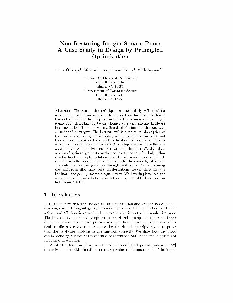
The �fth, and �nal, transformation step is the substitution of lower-level modulesfor the register and combinational assignments; the result is a structural descrip-tion of the integer square root algorithm which can readily be implemented inhardware, as shown in Figure 1.

ShiftReg4 is a shift register which shifts its contents two bits per clock cycle;the Done signal is simply its shift output. ShiftReg2, Mux, AddSub and Reg area shift register, multiplexer, adder/subtracter and register, respectively. SubAddis an adder/subtracter, but the sense of its mode bit makes it the opposite ofAddSub. The Hold element has the following substructure:

Hold {exact=Exact, zero=EqZero, rst=Init} ||

IsZero {out=EqZero, inp=DiffX} ||

Reg {out=DiffX, inp=DiffX'} ||

Mux {out=DiffX', in0=XIn, in1=DiffXTmp, ctl=Init} ||

AddSub {sum=DiffXTmp, in0=DiffX, in1=Delta, sub=ADD} ||

Neg {out=ADD, inp=$DiffX sub 16} ||

SubAdd {out=Delta, in0=YShift, in1=B, add=ADD} ||

ShiftReg2 {out=YShift, inp=YShift', shift=Exact} ||

Mux {out=YShift', in0=signal (%0),

in1=YShiftTmp div 2, ctl=Init} ||

SubAdd {out=YShiftTmp, in0=YShift, in1=2 * B, sub=ADD} ||

ShiftReg4 {out=B, shiftout=Done, in=signal initb, shiftbar=Init}

Fig. 1. Structural Description

fun Hold {exact=exact, zero=zero, rst=rst} =

let

val ExactReg = signal false

in

RegR {out=ExactReg, inp=exact, rst=rst} ||

Or2 {out=Exact, in0=zero, in1=ExactReg}

end

There are further opportunities for performing optimization in the imple-mentation of the lower level blocks. Analysis of the L2 algorithm reveals thatDelta is always positive, so we do not need its sign bit. This property can beused to save one bit in the AddSub used to compute Delta { only 16 bits arenow required. One bit can also be saved in the implementation of SubAdd; thevalue of the ADD signal can be shown to be identical to a latched version of thecarry output of a 16-bit SubAdd, provided the latch initially holds the value true.Figure 2 shows a block diagram of the hardware to implement the square rootalgorithm, which includes this optimization.

A number of other optimizations are not visible in the �gure. The ShiftReg4can be implemented by a ShiftReg2 half its width if we note that every secondbit of B is always zero. The two SubAdd blocks can each be implemented with onlya few AND and OR gates per bit, rather than requiring subtract/add modules,if we make use of some results concerning the contents of the B and YShift

registers.

To justify these optimizations we are obliged to prove that every second bitof B is always zero:

8i : 0 � i < n : :B2i+1

and that the corresponding bits of B and YShift cannot both be set:

8i : 0 � i < 2n::(Bi ^ YShifti)

Mux

Reg

IsZero HoldShift4

SubAdd SubAdd

AddSub

Reg

* 2

div 2

Mux

ShiftReg2

XInInit

Init

DiffX’

DiffXEqZero Exact

initb

B

Carry

Delta

ADD

YShift

YShift’

0

Done

YShiftTmp

Fig. 2. Square Root Hardware

and that the corresponding bits of $B * %2 and YShift cannot both be set:

8i : 1 � i < 2n::(Bi�1 ^ YShifti)

We have produced two implementations of the square root algorithm whichincorporate all these optimizations. The �rst was a full-custom CMOS layoutfabricated by Mosis, the second used Altera programmable logic parts. In thelatter case, the structural description was �rst translated to Altera's AHDLlanguage and then passed through Altera's synthesis software.

4 Discussion

We have described how to design and verify a subtractive, non-restoring integersquare root circuit by re�ning an abstract algorithmic speci�cation through sev-eral intermediate levels to yield a highly optimized hardware implementation.We have proved using Nuprl that the L0 algorithm performs the square rootfunction, and we have also used Nuprl to show how proving the �rst few levelsof re�nement (L0 to L1, L1 to L2) can be accomplished by transforming the toplevel proof in a way that preserves its validity.

This case study illustrates that rigorous reasoning about the high-level de-scription of an algorithm can establish properties which are useful even for bit-level optimization. Theorem provers provide a means of formally proving thedesired properties; a transformational approach to partitioning and optimiza-tion ensures that the properties remain relevant at the structural level. Each ofthe steps identi�ed in this paper can be mechanized with reasonable e�ort. Atthe bottom level, we have a library of veri�ed hardware modules that correspondto the modules in the HML structural description [AL94].

In many cases the transformations we applied depend for their justi�cationupon non-trivial properties of the square root algorithm: we are currently work-ing on formally proving these obligations. Some of our other transformations arepurely syntactic in nature and rely upon HML's semantics for their justi�ca-tion. We have not considered semantic reasoning in this paper { this is a currentresearch topic.

The algorithm we describe computes the integer square root. The algorithmand its implementation are of general interest because most of the algorithmsused in hardware implementations of oating-point square root are based on thealgorithm presented here. One di�erence is that most oating-point implementa-tions use a higher radix representation of operators. In the future, we will inves-tigate incorporating higher radix oating-point operations. We believe much ofthe reasoning presented here will be applicable to higher radix implementationsof square root as well.

Many of the techniques demonstrated in this case study are applicable tohardware veri�cation in general. Proof development systems are especially wellsuited for reasoning at high levels of abstraction and for relating multiple levelsof abstraction. Both of these techniques must be exploited in order to makeit feasible to apply formal methods to large scale highly optimized hardwaresystems. Top level speci�cations must be concise and intuitively capture thedesigners' natural notions of correctness (for example, arithmetic operations onunbounded integers), while the low level implementation must be easy to relateto the �nal implementation (for example, operations on bit-vectors). By applyinga transformational style of veri�cation as a design progresses from an abstractalgorithm to a concrete implementation, theorem proving based veri�cation canbe integrated into existing design practices.

Acknowledgements

This research is supported in part by the National Science Foundation undercontracts CCR-9257280 and CCR-9058180 and by donations from Altera Cor-poration. John O'Leary is supported by a Fellowship from Bell-Northern Re-search Ltd. Miriam Leeser is supported in part by an NSF Young InvestigatorAward. Jason Hickey is an employee of Bellcore. Mark Aagaard is supported bya Fellowship from Digital Equipment Corporation. We would like to thank PeterSoderquist for his help in understanding the algorithm and its implementations,Mark Hayden for his work on the proof of the algorithm, Shee Huat Chow andSer Yen Lee for implementing the VLSI version of this chip, and Michael Bertoneand Johanna deGroot for the Altera implementation.

References

[AL94] Mark D. Aagaard and Miriam E. Leeser. A methodology for reusable hard-ware proofs. Formal Methods in System Design, 1994. To appear.

[BJP93] Bhaskar Bose, Steve D. Johnson, and Shyamsundar Pullela. IntegratingBoolean veri�cation with formal derivation. In David Agnew, Luc Claesen,and Raul Camposano, editors, Computer Hardware Description Languages

and their Applications, IFIP Transactions A-32. Elsevier, North-Holland,1993.

[BV85] J. Bannur and A. Varma. A VLSI implementation of a square root algo-rithm. In IEEE Symp. on Comp. Arithmetic, pages 159{165. IEEE Comp.Soc. Press, Washington D.C., 1985.

[CGM86] Alberto Camilleri, Mike Gordon, and Tom Melham. Hardware veri�cationusing higher-order logic. In D. Borrione, editor, From HDL Descriptions to

Guaranteed Correct Circuit Designs. Elsevier, September 1986.[Flo63] Ivan Flores. The Logic of Computer Arithmetic. Prentice Hall, Englewood

Cli�s, NJ, 1963.[Lee92] Miriam E. Leeser. Using Nuprl for the veri�cation and synthesis of hard-

ware. In C. A. R. Hoare and M. J. C. Gordon, editors, Mechanized Reason-

ing and Hardware Design. Prentice-Hall International Series on ComputerScience, 1992.

[NS88] Paliath Narendran and Jonathan Stillman. Formal veri�cation of the sobelimage processing chip. In DAC, pages 211{217. IEEE Comp. Soc. Press,Washington D.C., 1988.

[OLLA92] John O'Leary, Mark Linderman, Miriam Leeser, and Mark Aagaard. HML:A hardware description language based on Standard ML. Technical ReportEE-CEG-92-7, Cornell School of Electrical Engineering, October 1992.

[OLLA93] John O'Leary, Mark Linderman, Miriam Leeser, and Mark Aagaard. HML:A hardware description language based on SML. In David Agnew, LucClaesen, and Raul Camposano, editors, Computer Hardware Description

Languages and their Applications, IFIP Transactions A-32. Elsevier, North-Holland, 1993.

[VCH94] D. Verkest, L. Claesen, and H. De Man A proof of the nonrestoring divisionalgorithm and its implementation on an ALU. Formal Methods in System

Design, 4(1):5{31, January 1994.

This article was processed using the LaTEX macro package with LLNCS style