Embed Size (px)
Citation preview

Non-Oscillatory Central Difference and Artificial Viscosity
Schemes for Relativistic Hydrodynamics
Peter Anninos and P. Chris Fragile
University of California,Lawrence Livermore National Laboratory, Livermore CA 94550
ABSTRACT
High resolution, non-oscillatory, central difference (NOCD) numerical
schemes are introduced as alternatives to more traditional artificial viscosity
(AV) and Godunov methods for solving the fully general relativistic hydrody-
namics equations. These new approaches provide the advantages of Godunov
methods in capturing ultra-relativistic flows without the cost and complication
of Riemann solvers, and the advantages of AV methods in their speed, ease of
implementation, and general applicability without explicitly using artificial vis-
cosity for shock capturing. Shock tube, wall shock, and dust accretion tests are
presented and compared against equivalent solutions from both AV and Godunov
based codes. In the process we address the accuracy of time-explicit NOCD and
AV methods over a wide range of Lorentz factors.
Subject headings: gravitation — hydrodynamics — relativity — methods: nu-
merical
1. Introduction
The earliest attempts at simulating relativistic flows in the presence of strong gravita-
tional fields are attributed to May and White (1966, 1967) who investigated gravitational
collapse in a one dimensional Lagrangian code using artificial viscosity (AV) methods (Von-
Neumann & Richtmyer 1950) to capture shock waves. Wilson (1972, 1979) subsequently
introduced an alternative Eulerian coordinate approach in multi-dimensional calculations,
using traditional finite difference upwind methods and artificial viscosity for shock capturing.
Since these earliest studies, AV methods have continued to be developed in their popularity
and applied to a variety of problems due largely to their general robustness (Hawley, Smarr,
& Wilson 1984a,b; Centrella & Wilson 1984; Anninos 1998). These methods are also com-
putationally cheap, easy to implement, and easily adaptible to multi-physics applications.
However, it has been demonstrated that problems involving high Lorentz factors (greater

– 2 –
than a few) are particularly sensitive to different implementations of the viscosity terms,
and can result in large numerical errors if solved using time explicit methods (Norman &
Winkler 1986).
Significant progress has been made in recent years to take advantage of the conser-
vational form of the hydrodynamics system of equations to apply Godunov-type methods
and approximate Riemann solvers to simulate ultra-relativistic flows (Eulderink & Mellema
1995; Banyuls et al. 1997; Font et al. 2000). Although Godunov-based schemes are ac-
cepted as more accurate alternatives to AV methods, especially in the limit of high Lorentz
factors, they are not infallible and should generally be used with caution. They may produce
unexpected results in certain cases that can be overcome only with specialized fixes or by
adding additional dissipation. A few known examples include the admittance of expansion
shocks, negative internal energies in kinematically dominated flows, ‘carbuncle’ effect in high
Mach number bow shocks, kinked Mach stems, and odd/even decoupling in mesh-aligned
shocks (Quirk 1994). Godunov methods, whether they solve the Riemann problem ex-
actly or approximately, are also computationally much more expensive than their simpler
AV counterparts, and more difficult to extend the system of equations to include additional
physics.
Hence we have undertaken this current study to explore an alternative approach of us-
ing high resolution, non-oscillatory, central difference (NOCD) methods (Jiang et al. 1998;
Jiang & Tadmor 1998) to solve the relativistic hydrodynamics equations. These new schemes
combine the speed, efficiency, and flexibility of AV methods with the advantages of the po-
tentially more accurate conservative formulation approach of Godunov methods, but without
the cost and complication of Riemann solvers and flux splitting.
The NOCD methods are implemented as part of a new code we developed called Cos-
mos, and designed for fully general relativistic problems. Cosmos is a collection of massively
parallel, multi-dimensional, multi-physics solvers applicable to both Newtonian and general
relativistic systems, and currently includes five different computational fluid dynamics (CFD)
methods, equilibrium and non-equilibrium primordial chemistry, photoionization, radiative
cooling, radiation flux-limited diffusion, radiation pressure, scalar fields, Newtonian external
and self gravity, arbitrary spacetime geometries, and viscous stress. The five hydrodynamics
methods include a Godunov (TVD) solver for Newtonian flows, two artificial viscosity codes
for general relativistic systems (differentiated by mesh or variable centering type: staggered
versus zone-centered), and two relativistic methods based on non-oscillatory central differ-
ence schemes (differentiated also by the mesh type: staggered versus centered in time and
space). The emphasis in the following sections is to review our particular implementations
of the AV and NOCD methods and compare results of various shock wave and accretion

– 3 –
test calculations with other published results. We also explore the accuracy of both AV and
NOCD methods in simulating ultra-relativistic shocks over a wide range of Lorentz factors.
2. Basic Equations
2.1. Internal Energy Formulation
Both of the artificial viscosity methods in Cosmos are based on an internal energy
formulation of the perfect fluid conservation equations. The equations are derived from the
4-velocity normalization uµuµ = −1, the conservation of baryon number ∇µ(ρuµ) = 0 for the
fluid rest mass density, the parallel component of the stress–energy conservation equation
uν∇µTµν = 0 for internal energy, the transverse component of the stress–energy conservation
equation (gαν + uαuν)∇µTµν = 0 for momentum, and an equation of state (eos) for the fluid
pressure P = P (ρ, ε), which for an ideal gas is P = (Γ− 1)e, where Γ is the adiabatic index
and e is the fluid internal energy density. For a perfect fluid, the stress-energy tensor is
T µν = ρhuµuν + Pgµν , (2-1)
where
h = 1 + ε +P
ρ= 1 + Γε (2-2)
is the relativistic enthalpy, ε is the specific internal energy, uµ is the contravariant 4-velocity,
and gµν is the 4-metric. The resulting equations can be written in flux conservative form as
(Wilson 1979)
∂D
∂t+
∂(DV i)
∂xi= 0, (2-3)
∂E
∂t+
∂(EV i)
∂xi+ P
∂W
∂t+ P
∂(WV i)
∂xi= 0 (2-4)
∂Sj
∂t+
∂(SjVi)
∂xi− SµSν
2S0
∂gµν
∂xj+√−g
∂P
∂xj= 0, (2-5)
where g is the determinant of the 4-metric, W =√−gu0 is the relativistic boost factor,
D = Wρ is the generalized fluid density, V i = ui/u0 is the transport velocity, Si = Wρhui
is the covariant momentum density, and E = We = Wρε is the generalized internal energy
density. We use the standard convention in which Greek (Latin) indices refer to 4(3)-space
components.
The system of equations (2-3) – (2-5) are complemented by two additional expressions
for V i and W that are convenient for numerical computation. Introducing a general tensor

– 4 –
form for artificial viscosity Qij (see section 3.1), and defining
M = ρhW = ρh√−gu0 = E + D + (P + tr[Qij ])W, (2-6)
the momentum can be expressed as Sµ = Muµ, and S0 is computed from the normalization
of the four–velocity SµSµ = −M2. The coordinate velocity then becomes V i = Si/S0 with
V 0 = 1. Also, the time component of the four–velocity u0 can be calculated from the
normalization uµuµ = u0V µSµ/M = −1, and used to derive the following expressions for W
W =−√−g M
SµV µ=
√−gS0
ρhW. (2-7)
The former expression (W = −√−g M/(SµVµ)) is used in the staggered mesh AV schemes
as it results in more accurate density and velocity jump conditions across shock fronts. The
latter is more convenient for the zone centered NOCD methods.
2.2. Conservative Energy Formulation
The second class of numerical methods presented in this paper (the NOCD schemes)
are based on a simpler conservative hyperbolic formulation of the hydrodynamics equations.
In this case, the equations are derived directly from the conservation of stress-energy
∇µT µν =1√−g
(√−gT µν)
,µ+ Γν
αµT µα = 0. (2-8)
Expanding (2-8) into time and space explicit parts yields the flux conservative equations for
general stress-energy tensors
∂(√−g T 0ν)
∂t+
∂(√−g T iν)
∂xi= Σν , (2-9)
with curvature source terms
Σν = −√−g T βγ Γνβγ . (2-10)
Substituting the perfect fluid stress tensor (2-1) into (2-9), and including baryon conservation
results in the following set of equations
∂D
∂t+
∂(DV i)
∂xi= 0, (2-11)
∂E∂t
+∂(EV i)
∂xi+
∂[√−g (g0i − g00V i) P ]
∂xi= Σ0, (2-12)
∂Sj
∂t+
∂(SjV i)
∂xi+
∂[√−g (gij − g0jV i) P ]
∂xi= Σj , (2-13)

– 5 –
where the variables D, V i, and g are the same as those defined in the internal energy
formulation. However, now
E = Wρhu0 +√−g g00P, (2-14)
Si = Wρhui +√−g g0iP, (2-15)
are the new expressions for energy and momenta.
It is convenient to express E and Si in terms of the internal energy formulation variables,
especially for initializing data
E =W 2
√−g
(D
W+ Γ
E
W
)+ (Γ− 1)
√−g g00 E
W, (2-16)
Si = giαSα + (Γ− 1)√−g g0i E
W, (2-17)
and reconstructing the equation of state
P = (Γ− 1)E
W(2-18)
=
(E√−g
W 2− D
W
)Γ− 1
Γ + (Γ− 1)g00(√−g/W )2
, (2-19)
where we have explicitly assumed an adiabatic gamma-law fluid.
3. Numerical Methods
Cosmos is a multi-dimensional (1, 2 or 3D) code that uses regularly spaced Cartesian
meshes for spatial finite differencing or finite volume discretization methods. Evolved vari-
ables are defined at the zone centers in the NOCD, TVD, and non-staggered AV methods. In
the staggered mesh AV method, variables are centered either at zone faces (the velocity V j
and momentum Sj vectors) or zone centers (all other scalar and tensor variables). Periodic,
reflection, constant in time, user-specified, and flat (vanishing first derivative) boundary
conditions are supported for all variables in the evolutions. The hydrodynamic equations in
both of the formalisms presented in §2 are solved with time-explicit, operator split methods
with second order spatial finite differencing. Single-step time integration and dimensional
splitting is used for both AV methods. The NOCD schemes use a second order predictor-
corrector time integration with dimensional splitting, and the TVD approach utilizes a third
order Runge-Kutta time integration with finite volume representations for source updates.
Since the main emphasis here is on relativistic hydrodynamics, the following discussion is
limited to presenting details relevant for the AV and NOCD schemes: the TVD method is
currently only Newtonian.

– 6 –
3.1. Artificial Viscosity
The order and frequency in which various source terms and state variables are updated
in the AV methods can affect the numerical accuracy, especially in high boost flows. The
following order composing a complete single cycle or timestep solution has been determined
to produce a reasonable compromise between cost and accuracy:
• Compute timestep ∆t from (3-1)
• Store current value of boost factor W
• Curvature
– compute pressure and sound speed from the ideal fluid equation of state:
P = (Γ− 1)E/W , Cs =√
ΓP/(ρh)
– evaluate scalar or tensor artificial viscosity Qij
– normalize velocity and update boost factor:
V i = Si/S0, using SµSµ = −M2 = −(D +E +PW +tr[Qij ]W )2 to first compute
S0;
then construct Sµ from gµν , S0, and the evolved Sj;
and finally use equation (2-7) to define the boost factor W = −√−gM/(SµV µ)
– update momentum, accounting for curvature:
Sj = SµSνgµν,j/(2S0), using second order finite differencing of gµν
• Artificial viscosity
– compute pressure
– normalize velocity, update W
– compute pressure and sound speed
– evaluate artificial viscosity components Qij
– update momentum and energy equations accounting for Qij :
E = −∑i,j Qij [∇i(WV j) +∇j(WV i)]/2, and Sj = −√−g∇iQij
• Compression
– compute pressure
– normalize velocity, update W
– compute pressure again

– 7 –
– update energy, accounting for compressional heating:
E = −P∇i(WV i)
• Pressure gradient
– compute pressure
– update momentum, accounting for pressure gradients:
Sj = −√−g∇jP
• Transport
– compute pressure
– normalize velocity, update W
– update transport terms in all variables:
D = −∇i(DV i), E = −∇i(EV i), and Sj = −∇i(SjVi)
• Boost factor
– compute pressure and sound speed
– normalize velocity, final update of W
– update energy, accounting for the variation of W in time:
E = −[P + (∑
i Q2ii/
∑i Qii)]W
• Update spacetime metric components gµν and gµν if time dependent
The highly nonlinear coupling of pressure and artificial viscosity to the state and kine-
matic variables through the Lorentz factor makes the relativistic equations much more dif-
ficult to solve than their Newtonian versions. It is for this reason that Norman & Winkler
(1986) adopted implicit methods to solve the special relativistic equations. It is also why we
have attempted to maintain a consistent and frequent update of the velocity normalization,
boost factor, pressure and artificial viscosity throughout the cycle.
To enforce stable evolutions, the timestep is defined for all hydro methods as the mini-
mum causality constraint over the entire mesh arising from the sound speed, fluid velocity,
magnitude of the artificial viscosity coefficient, and any other physics criteria introduced in
the calculation, say from scalar fields, radiation transport, gravity, etc... Also, since the
timesteps can be nonuniform, a final constraint is added to prevent ∆t from increasing by
more than 20% per timestep. In short,
∆tn+1 = min
[kc
Vmax, 1.2×∆tn
], (3-1)
– 8 –
where the superscript n refers to the discrete time level and the maximum velocity Vmax
(computed over all zones) accounts for local sound speed, fluid velocity, and viscous diffusion
Vmax = max
[Cs
min(dxi), max
( |V i|dxi
), 4kq2 max(|V i
,i|), 4kq2|∑
i
V i,i|
]. (3-2)
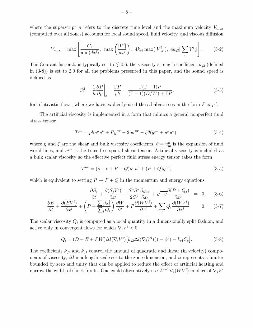
The Courant factor kc is typically set to . 0.6, the viscosity strength coefficient kq2 (defined
in (3-8)) is set to 2.0 for all the problems presented in this paper, and the sound speed is
defined as
C2s =
1
h
∂P
∂ρ
∣∣∣∣s
=ΓP
ρh=
Γ(Γ− 1)P
(Γ− 1)(D/W ) + ΓP. (3-3)
for relativistic flows, where we have explicitly used the adiabatic eos in the form P ∝ ρΓ.
The artificial viscosity is implemented in a form that mimics a general nonperfect fluid
stress tensor
T µν = ρhuµuν + Pgµν − 2ησµν − ξθ(gµν + uµuν), (3-4)
where η and ξ are the shear and bulk viscosity coefficients, θ = uµ;µ is the expansion of fluid
world lines, and σµν is the trace-free spatial shear tensor. Artificial viscosity is included as
a bulk scalar viscosity so the effective perfect fluid stress energy tensor takes the form
T µν = (ρ + e + P + Q)uµuν + (P + Q)gµν , (3-5)
which is equivalent to setting P → P + Q in the momentum and energy equations
∂Sj
∂t+
∂(SjVi)
∂xi− SµSν
2S0
∂gµν
∂xj+√−g
∂(P + Qj)
∂xj= 0, (3-6)
∂E
∂t+
∂(EV i)
∂xi+
(P +
∑i Q
2i∑
i Qi
)∂W
∂t+ P
∂(WV i)
∂xi+
∑i
Qi∂(WV i)
∂xi= 0. (3-7)
The scalar viscosity Qi is computed as a local quantity in a dimensionally split fashion, and
active only in convergent flows for which ∇iVi < 0
Qi = (D + E + PW )∆l(∇iVi)[kq2∆l(∇iV
i)(1− φ2)− kq1Cs
]. (3-8)
The coefficients kq2 and kq1 control the amount of quadratic and linear (in velocity) compo-
nents of viscosity, ∆l is a length scale set to the zone dimension, and φ represents a limiter
bounded by zero and unity that can be applied to reduce the effect of artificial heating and
narrow the width of shock fronts. One could alternatively use W−1∇i(WV i) in place of ∇iVi

– 9 –
in (3-8), which we find to be effective at preventing excessively large jump errors and helps
stabilize solutions in highly relativistic shock tube and wall shock calculations.
A more general tensor version of artificial viscosity is also implemented for convergent
flows to the form (Tscharnuter & Winkler 1979)
Qij = (D + E + PW )∆l[kq2∇kV
k∆l − kq1Cs
] [1
2(∇iV
j +∇jVi)− c
3∇kV
kδij
], (3-9)
where c is a constant defined as zero or unity depending on whether the viscosity tensor
should be traceless or not, and δij is the Kronecker delta. The equations for energy and
momentum with a tensor viscosity are similar to (3-6) and (3-7) except in the way two of
the viscosity terms are computed
∂Sj
∂t+
∂(SjVi)
∂xi− SµSν
2S0
∂gµν
∂xj+√−g
∂P
∂xj+√−g
∂Qjk
∂xk= 0,(3-10)
∂E
∂t+
∂(EV i)
∂xi+
(P +
∑i Q
2ii∑
i Qii
)∂W
∂t+ P
∂(WV i)
∂xi+
1
2
∑i,j
Qij
(∂(WV i)
∂xj+
∂(WV j)
∂xi
)= 0.(3-11)
The scalar form of artificial viscosity (3-8) is used in all the tests presented in this paper.
The transport step is solved in a directionally split, flux conservative manner. For
example, considering advection of the density field along the x-axis in a staggered mesh
scheme, the solution to D = −∇x(DV x) is written
Dn+1i = Dn
i −∆tn
∆x
[Di+1Vi+1 − DiVi
], (3-12)
where Vi+1 is the face-centered velocity between zones i and i + 1, and Di is a first order
monotonic Taylor’s approximation of Di from the upwind cell center to the advection control
volume center
Di =
[1
2+ sign
(1
2, Vi
)] [Di−1 +
(∆x− Vi∆t)
2(∇xD)i−1
]+
[1
2− sign
(1
2, Vi
)][Di − (∆x + Vi∆t)
2(∇xD)i
]. (3-13)
Equation (3-13) automatically detects the upwind cell from the sign of the velocity V . Here,
sign(1/2, Vi) is fortran notation for ±1/2, depending on the sign of Vi. High order van Leer
(1977) monotonic interpolation is used to reconstruct local gradients (∇xD)i and prevent
spurious oscillations near regions of sharp gradients
(∇xD)i =
[1
2+ sign
(1
2, ∆Di ∆Di−1
)](2∆Di ∆Di−1
∆Di + ∆Di−1 + δ
). (3-14)

– 10 –
The constant δ � 1 is introduced to prevent numerical overflow, and ∆Di = (Di+1−Di)/∆x
are the mesh aligned gradients centered on the cell faces. Similar expressions can easily be
derived for zone-centered variables on nonstaggered meshes by face-averaging the velocities,
and for face-centered variables on staggered meshes by shifting the spatial indices and control
volumes appropriately.
3.2. Non-oscillatory Central Difference Schemes
Considering the simplicity of equations (2-11) - (2-13), an obvious benefit of the NOCD
approach is that, unlike the AV approach, it is not expected to be particularly sensitive to
any ordering of operator updates since the method basically just solves a single first order
operator equation with external sources. We have implemented two variations of this method:
the first with non-staggered spatial and temporal meshes with second order reconstruction,
and the second with time-staggered meshes in which the variables are updated on a mesh
shifted in time to center the solution properly to second order. A summary of the solver
sequence for this class of methods is:
• Compute timestep ∆t from (3-1),
redefine ∆t → ∆t/2 for the 2-step, subcycled, staggered mesh scheme
• Curvature
– compute pressure from the ideal fluid equation of state:
P = (Γ− 1)[E√−g/(W 2)−D/W ]/[Γ + (Γ− 1)g00(√−g/W )2]
– update energy and momentum, accounting for curvature:
E = Σ0 and Sj = Σj , using second order finite differencing for metric derivatives
• Flux operator
– compute pressure from eos
– normalize velocity and update boost factor:
V i = Si/S0, using SµSµ = −M2 = −[(E −√−gg00P )√−g/W ]2 and
Si = Si −√−gg0iP to first compute S0, then the boost factor W =√−gS0/M
– compute pressure
– update all variables ω ≡ (D, E, Sj),
accounting for flux-conservative gradient terms in equations (2-11) - (2-13):
ω = −∇i[ωV i +√−gP (giα − g0αV i)]

– 11 –
– if the mesh is nonstaggered in time:
perform interpolations to recenter variables on the original unstaggered mesh
ωn+1j = (ωn+1
j−1/2 + ωn+1j+1/2)/2 + (ωn+1′
j−1/2 − ωn+1′j+1/2)/8
• If the mesh is staggered:
– repeat curvature and flux steps to evolve solution from t = tn+1/2 to tn+1
– shift array indices to realign final coordinates at tn+1 with
initial coordinates at tn by ωi,j,k = ωi−1,j−1,k−1
• Update spacetime metric components gµν and gµν if time dependent
Two essential assumptions built into this method are that the cell-averaged solutions can
be reconstructed as MUSCL-type piece-wise linear interpolants, and that the flux integrals
are defined and evaluated naturally on staggered meshes. Since we adopt directional splitting
for multi-dimensional problems, the basic discretization scheme used to solve equations (2-
11) - (2-13) can be derived from a simple one-dimensional, first order model equation of the
form
∂ω
∂t+
∂f(ω)
∂x= 0, (3-15)
where ω represents any of the density, energy or momentum variables, and f(ω) is the
associated flux. A formal solution to (3-15) can be written over a single time cycle (tn → tn+1)
on a staggered mesh as
ωj+1/2(tn+1) = ωj+1/2(t
n)− ∆t
∆x
[1
∆t
∫ tn+1
tnf(ωj+1(τ))dτ − 1
∆t
∫ tn+1
tnf(ωj(τ))dτ
]. (3-16)
Introducing the notation ω′j = ωj+1−ωj−1, the average of the piece-wise linearly reconstructed
solutions at the staggered positions ωj+1/2(tn) in (3-16) is given by
ωj+1/2 =1
2(ω+
j+1/2 + ω−j+1/2) =
1
2(ωj + ωj+1) +
1
8(ω′
j − ω′j+1), (3-17)
where ω±j+1/2 refer to the piecewise linearly interpolated solutions from the upwind and
downwind cell centers
ω+j+1/2 = ωj+1 − 1
4(ωj+2 − ωj), (3-18)
ω−j+1/2 = ωj +
1
4(ωj+1 − ωj−1). (3-19)

– 12 –
Considering that the time averaged integrals in (3-16) can be approximated using mid-
point values
1
∆t
∫ tn+1
tnf(ωj(τ))dτ ∼ f(ωj(t
n+1/2)), (3-20)
immediately suggests a two step predictor-corrector procedure to solve (3-15): the state
variables are predicted at t = tn+1/2 by
ωn+1/2j = ωn
j −∆t
2∆xf ′(ωj), (3-21)
then corrected on the staggered mesh by
ωn+1j+1/2 =
1
2(ωn
j + ωnj+1) +
1
8(ω′
j − ω′j+1)−
∆t
∆x
[f(ω
n+1/2j+1 )− f(ω
n+1/2j )
], (3-22)
where we have also substituted (3-17) for ωj+1/2(tn) in (3-16). Equations (3-21) and (3-
22) represent the complete single cycle solution averaged on a staggered mesh. The mesh
indices can be brought back into alignment by setting ∆t → ∆t/2, performing two time cycle
updates (computing ωn+1/2j+1/2 then ωn+1
j+1 ) to time tn+1 = tn +∆t, and re-center the solution on
the original zone positions by shifting the array indices as ωj = ωj−1.
As an alternative to mesh staggering, the solution after applying the corrector step can
be reconstructed directly back to the nonstaggered cell centers by a second order piece-wise
linear extrapolation
ωn+1j =
1
2(ωn+1
j−1/2 + ωn+1j+1/2) +
1
8(ωn+1′
j−1/2 − ωn+1′j+1/2), (3-23)
to yield for the final single timestep solution
ωn+1j =
1
4(ωn
j−1 + 2ωnj + ωn
j+1)−1
16
(ωn′
j+1 − ωn′j−1
)− ∆t
2∆x
[f(ω
n+1/2j+1 )− f(ω
n+1/2j−1 )
]− 1
8
(ωn+1′
j+1/2 − ωn+1′j−1/2
). (3-24)
We have found no substantial differences between the staggered and unstaggered approaches
in all the test calculations we have performed. Hence all subsequent results presented in this
paper from this class of algorithms are derived with the nonstaggered mesh method using
(3-21) and (3-24).
One final important element of this method is that all gradients (of either the state
variables ω′j or fluxes f ′(ωj)) must be processed and limited for monotonicity in order to
guarantee non-oscillatory behavior. This is accomplished with either the minmod limiter
ω′j = max
(0, min
(1,
ωj − ωj−1
ωj+1 − ωj
))(ωj+1 − ωj) , (3-25)

– 13 –
or the van Leer limiter
ω′j =
[ |(ωj − ωj−1)/(ωj+1 − ωj)|+ (ωj − ωj−1)/(ωj+1 − ωj)
1 + |(ωj − ωj−1)/(ωj+1 − ωj)|]
(ωj+1 − ωj) , (3-26)
which satisfy the TVD constraints with appropriate Courant restrictions, although we note
that steeper limiters can yield undesirable results especially in under-resolved high boost
shock tube calculations.
4. Code Tests
4.1. Relativistic Shock Tube
We begin testing the staggered AV and nonstaggered NOCD methods with one of the
standard problems in fluid dynamics, the shock tube. This test is characterized initially by
two different fluid states separated by a membrane. At t = 0 the membrane is removed and
the fluid evolves in such a way that five distinct regions appear in the flow: an undisturbed
region at each end, separated by a rarefaction wave, a contact discontinuity, and a shock
wave. This problem only checks the hydrodynamical elements of the code, as it assumes a
flat background metric. However, it provides a good test of the shock-capturing properties
of the different methods since it has an exact solution (Thompson 1986) against which the
numerical results can be compared.
Two cases of the shock tube problem are considered first: moderate boost (W = 1.43)
and high boost (W = 3.59) shock waves. In the moderate boost case, the initial state is
specified by ρL = 10, PL = 13.3, and VL = 0 to the left of the membrane and ρR = 1,
PR = 10−6, and VR = 0 to the right. In the high boost case, ρL = 1, PL = 103, VL = 0,
and ρR = 1, PR = 10−2, VR = 0. In both cases, the fluid is assumed to be an ideal gas with
Γ = 5/3, and the integration domain extends over a unit grid from x = 0 to x = 1, with
the membrane located at x = 0.5. Most of the AV shock tube results presented here were
run using the scalar artificial viscosity with a quadratic viscosity coefficient kq2 = 2.0, linear
viscosity coefficient kq1 = 0.3, and Courant factor kc = 0.6. A couple of the highest boost
runs presented in Table 3 are the only exceptions. In these cases the viscosity coefficients were
kept the same but the Courant factor was varied as needed to maintain stability. We have
carried out these tests in one, two and three dimensions, lining up the interface membrane
along the main diagonals in multi-dimensional runs. For the NOCD method we use kc = 0.3
and the minmod limiter which gives smoother and more robust results than the steeper
limiters in simulations of under-resolved highly relativistic shocks.
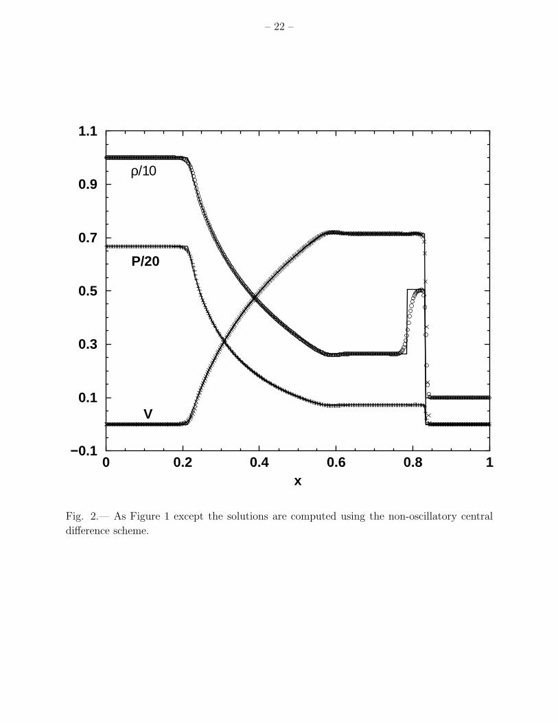
Figures 1 & 2 show spatial profiles of the moderate boost results at time t = 0.4 on a

– 14 –
grid of 400 uniformly spaced zones using the AV and NOCD methods respectively. Figures 3
& 4 show the corresponding solutions of both AV and NOCD methods for the high boost test
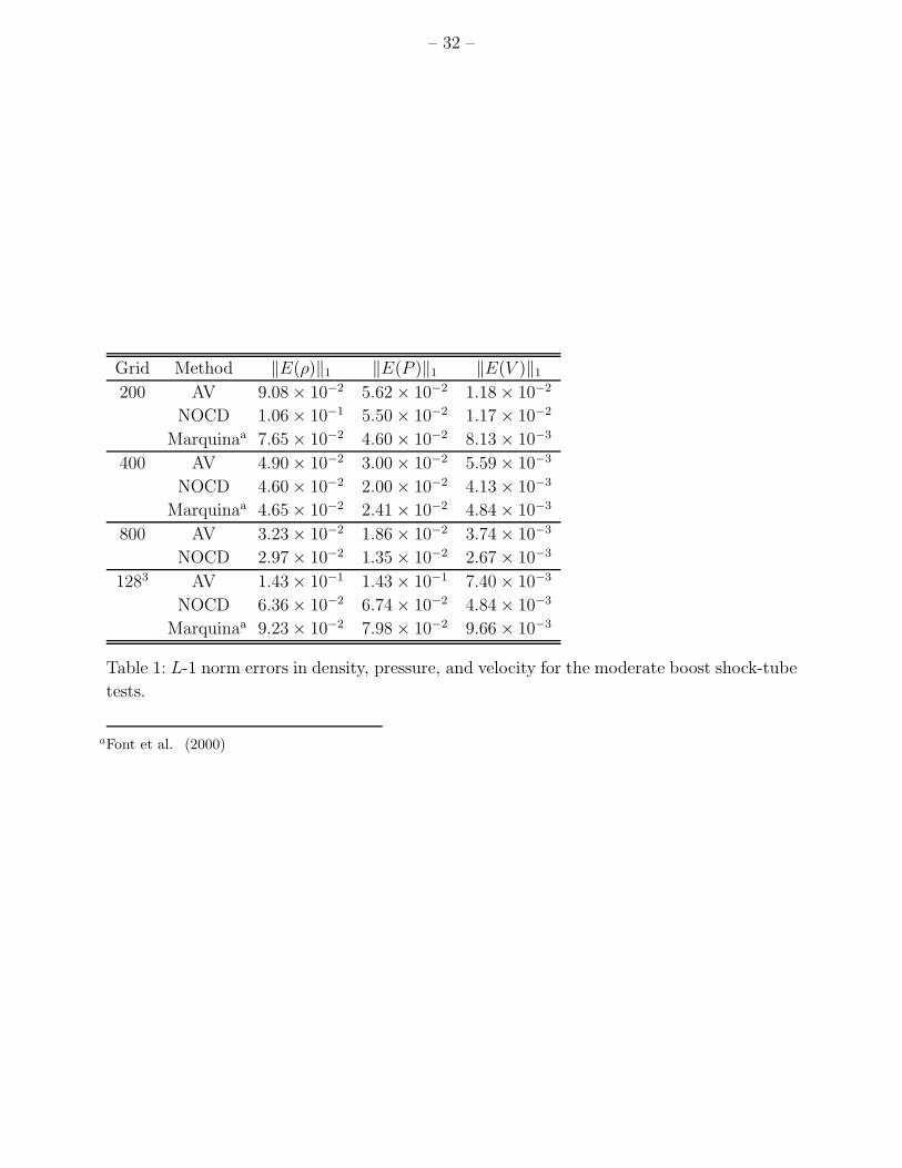
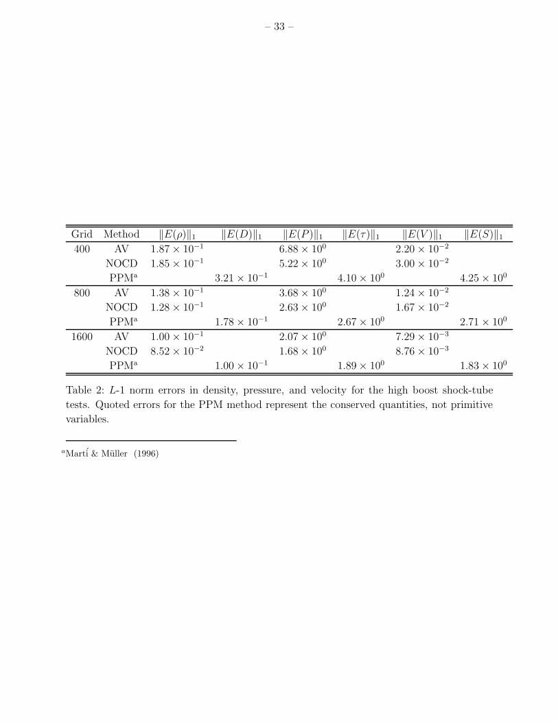
using a higher resolution grid with 800 zones at time t = 0.36. Tables 1 & 2 summarize the
errors in the primitive variables ρ, P , and V for different grid resolutions and CFD methods
using the L-1 norm (i.e., ‖E(a)‖1 =∑
i,j,k ∆xi∆yj∆zk|ani,j,k − An
i,j,k|, where ani,j,k and An
i,j,k
are the numerical and exact solutions, respectively, and for 1D problems the orthogonal grid
spacings are set to unity). Included in Table 1 for comparison are the errors reported by Font
et al. (2000) using Marquina’s approximate Riemann solver (Donat & Marquina 1996).
They also tested the Roe and Flux-split approximate solvers and achieved similar results as
with Marquina’s method, so we do not include those numbers here. We find the errors in
Table 1 are quite comparable between all three methods with convergence rates just under
first order as expected for shock capturing methods. For the high boost case in Table 2,
our errors are comparable to those reported by Marti & Muller (1996) for the same shock
tube simulation using an extended high order piecewise parabolic method (PPM)(Colella
& Woodward 1984) with an exact Riemann solver. However, we note that their published
errors are for the conserved quantities (generalized fluid density D, generalized energy density
τ = ρhW 2−P −D, and covariant momentum density S) rather than the primitive variables
we report. Their results are included in Table 2. We also note that the slightly larger errors
in the 3D AV results of Table 1 are due primarily to boundary effects (particulary at the
grid corners) and not to shock capturing differences. In fact, errors computed only along the
main diagonal are about the same for the NOCD and AV methods.
Table 3 shows the mean-relative errors (defined as εrel(a) =∑
i,j,k |ani,j,k−An
i,j,k|/∑
i,j,k |Ani,j,k|,
where again ani,j,k and An
i,j,k are the numerical and exact solutions, respectively) in the prim-
itive variables over a range of boost factors using 800 zones to cover the same unit domain.
The different boost factors are established by systematically increasing the original value of
PL over the moderate boost case. These errors are also displayed graphically in Figure 5,
comparing the AV and NOCD methods up to about the maximum boost for which the AV
approach can be pushed reliably at these grid resolutions. The increasing trend (with boost)
in error reflects the stronger nonlinear coupling through the fluid velocity and the narrower
and steeper leading shock plateau as evidenced in the density plots. At 800 zone resolution,
the leading density plateau for the high boost case is covered by fewer than nine cells in
the analytic solution, compared to about thirty-six zones for the corresponding moderate
boost calculation. For shock velocities greater than about V ∼ 0.95, the AV results become
increasingly unstable and uncertain with respect to parameter choices (resolution, Courant
factor, viscosity strengths, etc...). However, over the range in which AV results are robust,
the errors are comparable between the AV, NOCD, and Godunov methods.

– 15 –
4.2. Relativistic Wall Shock
A second test presented here is the wall shock problem involving the shock heating of
cold fluid hitting a wall at the left boundary (x = 0) of a unit grid domain. The initial
data are set up to be uniform across the grid with adiabatic index Γ = 4/3, pre-shocked
density ρ1 = 1, pre-shocked pressure P1 = 7.63× 10⁻⁶, and velocity V1 = −vinit = −(1− ν),
where ν < 1 is the infall velocity parameter. When the fluid hits the wall a shock forms and
travels to the right, separating the pre-shocked state composed of the initial data and the
post-shocked state with solution in the wall frame
VS =ρ1W1V1
ρ2 − ρ1W1, (4-1)
P2 = ρ2(Γ− 1)(W1 − 1), (4-2)
ρ2 = ρ1
[Γ + 1
Γ− 1+
Γ
Γ− 1(W1 − 1)
], (4-3)
where VS is the velocity of the shock front, and the pre-shocked energy and post-shocked
velocity were both assumed negligible (ε1 = V2 = 0). To facilitate a direct comparison
between our results and the Genesis code of Aloy, Ibanez, & Marti (1999) (which again uses
Marquina’s approximate Riemann solver) all of the results shown in the figures and tables,
unless noted otherwise, were performed on a 200 zone uniformly spaced mesh and ran to a
final time of t = 2.0. Also, for the NOCD methods, the courant factor is set to kc = 0.3, and
we use the van Leer limiter for gradient calculations, which generally gives smaller errors
when compared to the more diffusive minmod limiter (about a 30% reduction for the lower
boost cases we have tried). For the AV methods, we use the scalar viscosity with kc = 0.6,
kq1 = 0.3, and kq2 = 2.0 for all the runs.
Figures 6 & 7 show spatial profiles for the case with initial velocity vinit = 0.9 and 200
zones for the AV and NOCD methods, respectively. Table 4 summarizes the L-1 norm errors
in both methods as a function of grid resolution. The values given in parentheses are the
contributions to the total error in the first twenty zones from the reflection wall at x = 0.
These numbers clearly indicate a disproportionate error distribution from wall heating, an
effect that is especially evident in the AV results. Excluding this contribution may give a
more accurate assessment of each method’s ability to resolve the actual shock profile.
Figure 8 plots the mean-relative errors (using 200 zones) in density, which are generally
greater than errors in either the pressure or velocity, as a function of boost factor up to
about the maximum boost that the AV methods can be run accurately. Although we are
not able to extend the AV method reliably beyond vinit ∼ 0.97, the NOCD methods, on the
other hand, are substantially more robust. In fact, as shown in Table 5 and Figure 9, the
NOCD schemes can be run up to arbitrarily high boost factors with stable mean relative

– 16 –
errors, typically less than two percent with no significant increasing trend. These errors are
generally smaller than those quoted by Aloy, Ibanez, & Marti (1999). We note that the
errors for the AV method presented in Figure 8 and Table 5 can be improved significantly
by either lowering the Courant factor or increasing the viscosity coefficients. For example,
decreasing kc from 0.6 to 0.3, or increasing kq2 from 2 to 3 for the case vinit = 0.95 reduces
the L-1 norm in density from 0.116 to 0.048 and 0.033, respectively. We have also been able
to run wall shock tests with the AV method at slightly higher boosts than shown in Table
5 by choosing different parameter combinations (e.g., kc = 0.2, kq1 = 1.0 and 400 zones can
evolve flows with vinit = 0.99 fairly accurately). However, rather than adjusting parameters
to achieve the best possible result for each specific problem, we have opted to keep numerical
parameters constant between code tests, boost factors, and numerical methods.
4.3. Black Hole Accretion
As a test of hydrodynamic flows in spacetimes with nontrivial curvature, we consider
radial accretion of an ideal fluid onto a compact, strongly gravitating object, in this case a
Schwarzschild black hole. The fluid will accrete onto the compact object along geodesics, thus
allowing the general relativistic components of our codes to be tested against a well-known
analytic stationary solution. Assuming a perfect fluid in isotropic Schwarzschild coordinates
ds2 = −(
1−M/2ρ
1 + M/2ρ
)2
dt2 +
(1 +
M
2ρ
)4 (dx2 + dy2 + dz2
), (4-4)
where ρ =√
x2 + y2 + z2 is the isotropic radius, the exact solution to this problem is depen-
dent on a single parameter, the gravitational binding energy (u0). In terms of this parameter
(which we set to u0 = −1 in our tests), the solution can be written
W =√−g g00u0, (4-5)
D =CD
ρ2V ρ, (4-6)
E =CE
W Γ−1(ρ2V ρ)Γ, (4-7)
V ρ = −uρ
u0= − 1
g00u0
√−gρρ(1 + g00u2
0), (4-8)
where W is the boost factor, V ρ is the radial infall velocity in isotropic radial coordinates,
D is the generalized density in isotropic Cartesian coordinates, E is the generalized internal
energy in isotropic Cartesian coordinates, Γ = 5/3 is the adiabatic index, and CD and CE
are constants of integration which we set to CD = 1 and CE = CD/100 in the simulations.

– 17 –
The computational domain for this problem is constructed to be (5M)3 (where M = 1
is the black hole mass) and centered along the z-axis with −2.5M ≤ (x, y) ≤ 2.5M . In
the z-direction the inner boundary zone z = zmin is defined to lie outside the event horizon
at zmin = 1.5M in isotropic coordinates to guarantee all boundary zones are outside the
horizon, and extends to z = zmax = 6.5M along the x = y = 0 line. Calculations are carried
out on different resolution grids, ranging from 163 to 643 to check code convergence. All
variables are initially set to negligible values throughout the interior domain (D = 10−2,
E = DCE/CD, W = 1, and Si = V i = 0), and the static analytic solutions are specified
as outer boundary conditions at all times. Along the inner z boundary, outflow conditions
are maintained by simply setting the first derivatives of all variables to zero at the end of
each timestep. Thus fluid flows onto the computational grid from all of the analytically-
specified (inflow) boundaries, and exits from the lower z-plane closest to the black hole. All
results presented here were generated from simulations run until steady-state was achieved
at t = 50M , and numerical parameters are defined as in previous tests, namely kc = 0.6,
kq1 = 0, kq2 = 2.0 in the AV runs, and kc = 0.3 in the NOCD results. Table 6 summarizes
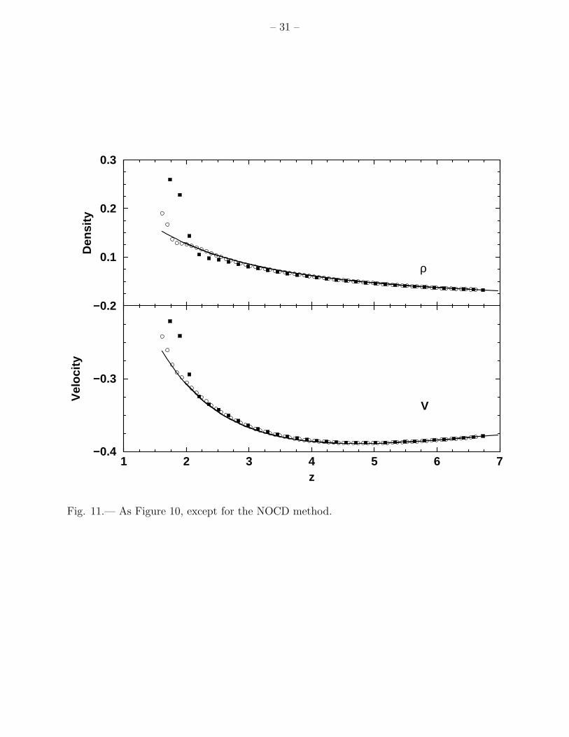
the global mean-relative errors in both methods as a function of grid resolution. Figures 10
& 11 show spatial profiles of density and velocity along the z-axis for 323 and 643 zones for
the AV and NOCD methods, respectively.
Although the numerical results in Table 6 converge to the analytic solution with grid
resolution, they converge at a rate between first and second order due in part to the treatment
of boundary conditions and time discretization errors. In particular, comparing the analytic
and numerical solutions, we find that maximum relative errors occur near the event horizon
along the inner z-boundary. For the AV method, the maximum relative errors for density
and velocity with 643 zones are 9.16% and 2.49%, respectively, compared to global mean-
relative errors of 1.36% and 0.63%. For the NOCD method, the maximum relative errors
are 24.4% and 7.42%, compared to global mean-relative errors of 2.11% and 0.14%. The
global errors in both methods, in spite of being computed on a nonsymmetric Cartesian
mesh, are comparable to those reported by other authors. For instance, Hawley, Smarr, &
Wilson (1984b) saw relative errors of 1-3% in density and velocity near the horizon using
an artificial viscosity code on a 25 × 10 cylindrical grid. Banyuls et al. (1997) saw mean
relative errors of 2.67% and 0.99% using a Godunov-type method on a 200×5 spherical grid.
Also, decreasing the Courant factor from kc = 0.6 to 0.2 reduces the errors in both AV and
NOCD methods by about a factor of three, consistent with first order time discretization,
and increases the rate of spatial convergence closer to second order.
– 18 –
5. Conclusion
We have developed new artificial viscosity and non-oscillatory central difference nu-
merical hydrodynamics schemes as integral components of the Cosmos code framework for
performing fully general relativistic calculations of strong field flows. These methods have
been discussed at length here and compared also with published state-of-the-art Godunov
methods on their abilities to model shock tube, wall shock and black hole accretion problems.
We find that for shock tube problems at moderate to high boost factors, with velocities up to
V ∼ 0.95 − 0.99, the artificial viscosity methods compare quite favorably with the NOCD
methods, the Godunov methods using the Marquina, Roe, or Flux-split approximate Rie-
mann solvers, and the piecewise parabolic method with an exact Riemann solver. However,
they tend to become unstable or at least highly sensitive to parameters and generally unreli-
able at higher boosts (V & 0.95). On the other hand, NOCD methods can easily be extended
to ultra-relativistic velocities (1−V < 10−11) as demonstrated by the wall shock tests carried
out in this paper, and are comparable in accuracy over the entire range of velocities we have
simulated to the more standard but complicated Riemann solver codes. NOCD schemes thus
provide a robust new alternative to simulating relativistic hydrodynamical flows since they
offer the same advantages of Godunov methods in capturing ultra-relativistic flows but with-
out the cost and complication of Riemann solvers or flux splitting. They also provide all the
advantages of AV methods in their speed, ease of implementation, and general applicability
without explicitly using artificial viscosity for shock capturing.
This work was performed under the auspices of the U.S. Department of Energy by
University of California, Lawrence Livermore National Laboratory under Contract W-7405-
Eng-48.

– 19 –
REFERENCES
Aloy, M. A., Ibanez, J. M., and Marti, J. M. 1999, ApJS, 122, 151
Anninos, P. 1998, Phys. Rev. D, 58, 064010
Banyuls, F., Font, J. A., Ibanez, J. M., Marti, J. M. and Miralles, J. A. 1997, ApJ, 476, 221
Centrella, J. and Wilson, J. R. 1984, ApJS, 54, 229
Colella, P. and Woodward, P. R. 1984, J. Comput. Phys., 54, 174
Donat, R. and Marquina, A. 1996, J. Comput. Phys., 125, 42
Eulderink, F. and Mellema, G. 1995, Astron. Astrophys. Suppl. Ser., 110, 587
Font, J. A., Miller, M., Suen, W. and Tobias, M. 2000, Phys. Rev. D, 61, 044011
Hawley, J. F., Smarr, L. L. and Wilson, J. R. 1984, ApJ, 277, 296
Hawley, J. F., Smarr, L. L. and Wilson, J. R. 1984, ApJS, 55, 211
Jiang, O.-S., Levy, D., Lin, C.-T., Osher, S. and Tadmor, E. 1998, SIAM J. Numer. Anal.,
35, 2147
Jiang, O.-S. and Tadmor, E. 1998, SIAM J. Sci. Comput., 19, 1892
Marti, J. and Muller, E. 1996, J. Comput. Phys., 123, 1
May, M. M. and White, R. H. 1966, Phys. Rev. D, 141, 1232
May, M. M. and White, R. H. 1967, Meth. Computat. Phys., 7, 219
Norman, M. L. and Winkler, K.-H. A. 1986, in Astrophysical Radiation Hydrodynamics, ed.
M. L. Norman & K.-H. A. Winkler (NATO ASI ser. C, 188) (Dordrecht:Reidel), 449
Quirk, J. J., 1994, Int. J. for Numerical Methods in Fluids, 18, 555
Thompson, K. W. 1986, J. Fluid Mech., 171, 365
Tscharnuter, W.-M. and Winkler, K.-H. 1979, Comput. Phys. Comm., 18, 171
van Leer, B. 1977, J. Comput. Phys., 23, 276
VonNeumann, J. and Richtmyer, R. D. 1950, J. Appl. Phys., 21, 232
Wilson, J. R. 1972, ApJ, 173, 431

– 20 –
Wilson, J. R., in Sources of Gravitational Radiation, edited by L. Smarr (Cambridge Uni-
versity Press, Cambridge, England, 1979)
AAS LATEX macros v5.0.

– 21 –
0 0.2 0.4 0.6 0.8 1x
−0.1
0.1
0.3
0.5
0.7
0.9
1.1
ρ/10
P/20
V
Fig. 1.— Normalized results for the moderate boost shock tube test using artificial viscosity
for shock capturing and 400 zones to cover a unit grid. The solution is shown at time t = 0.4.
– 22 –
0 0.2 0.4 0.6 0.8 1x
−0.1
0.1
0.3
0.5
0.7
0.9
1.1
ρ/10
P/20
V
Fig. 2.— As Figure 1 except the solutions are computed using the non-oscillatory central
difference scheme.

– 23 –
0 0.2 0.4 0.6 0.8 1x
−0.2
0
0.2
0.4
0.6
0.8
1
1.2
1.4
P/1000
ρ/10
V
Fig. 3.— Results at time t = 0.36 for the high boost shock tube test using artificial viscosity
and 800 zones.

– 24 –
0 0.2 0.4 0.6 0.8 1x
−0.2
0
0.2
0.4
0.6
0.8
1
1.2
V
ρ/10
P/1000
Fig. 4.— As Figure 3 but with the non-oscillatory central difference scheme.

– 25 –
1 2 3 4boost factor
10−3
10−2
10−1
mea
n re
lativ
e er
ror
in d
ensi
ty
AVNOCD
Fig. 5.— Mean relative errors in density for both the AV and NOCD methods as a function
of boost for the relativistic shock tube problem. All calculations were run using 800 zones
up to time t = 0.36.

– 26 –
0 0.2 0.4 0.6 0.8 1x
−1
−0.8
−0.6
−0.4
−0.2
0
0.2
0.4
0.6
0.8
1
V=−0.9c
P/10
ρ/15
Fig. 6.— Results for the relativistic wall shock test with 200-zone resolution and infall
velocity V = −0.9c using artificial viscosity. The solution is shown at time t = 2.0.

– 27 –
0 0.2 0.4 0.6 0.8 1x
−1
−0.8
−0.6
−0.4
−0.2
0
0.2
0.4
0.6
0.8
1
V=−0.9c
P/10
ρ/15
Fig. 7.— As Figure 6 but for the NOCD scheme.

– 28 –
1 2 3 4 5boost factor
10−3
10−2
10−1
100
mea
n re
lativ
e er
ror
in d
ensi
ty
AVNOCD
Fig. 8.— Mean relative errors in density for both the AV and NOCD methods as a function
of boost for the relativistic wall shock problem. All calculations were run using 200 zones
up to time t = 2.0. The AV results can be signiciantly improved and brought closer in
alignment with the NOCD results by simply reducing the Courant factor or increasing the
viscosity coefficients over the standard values we have chosen for all the tests.

– 29 –
0 0.2 0.4 0.6 0.8 1x
100
101
102
103
104
105
106
Den
sity
V=−0.9c
V=−0.999c
V=−0.99999c
V=−0.9999999c
V=−0.999999999c
V=−0.99999999999c
Fig. 9.— Density plots for different infall velocities in the wall shock test using the NOCD
method. The resolution is 200 zones and the displayed time is t = 2.0.

– 30 –
1 2 3 4 5 6 7z
−0.4
−0.3
Vel
ocity
0.1
0.2
Den
sity
ρ
V
Fig. 10.— Plots of density and velocity along the z-axis for the dust accretion problem using
the AV method. The filled squares and open circles correspond to resolutions of 323 and 643,
respectively. The solid line is the analytic solution. The displayed time is t = 50M .
– 31 –
1 2 3 4 5 6 7z
−0.4
−0.3
−0.2
Vel
ocity
0.1
0.2
0.3
Den
sity
ρ
V
Fig. 11.— As Figure 10, except for the NOCD method.
– 32 –
Grid Method ‖E(ρ)‖1 ‖E(P )‖1 ‖E(V )‖1
200 AV 9.08× 10⁻² 5.62× 10⁻² 1.18× 10⁻²
NOCD 1.06× 10⁻¹ 5.50× 10⁻² 1.17× 10⁻²
Marquinaa 7.65× 10⁻² 4.60× 10⁻² 8.13× 10⁻³
400 AV 4.90× 10⁻² 3.00× 10⁻² 5.59× 10⁻³
NOCD 4.60× 10⁻² 2.00× 10⁻² 4.13× 10⁻³
Marquinaa 4.65× 10⁻² 2.41× 10⁻² 4.84× 10⁻³
800 AV 3.23× 10⁻² 1.86× 10⁻² 3.74× 10⁻³
NOCD 2.97× 10⁻² 1.35× 10⁻² 2.67× 10⁻³
1283 AV 1.43× 10⁻¹ 1.43× 10⁻¹ 7.40× 10⁻³
NOCD 6.36× 10⁻² 6.74× 10⁻² 4.84× 10⁻³
Marquinaa 9.23× 10⁻² 7.98× 10⁻² 9.66× 10⁻³
Table 1: L-1 norm errors in density, pressure, and velocity for the moderate boost shock-tube
tests.
aFont et al. (2000)
– 33 –
Grid Method ‖E(ρ)‖1 ‖E(D)‖1 ‖E(P )‖1 ‖E(τ)‖1 ‖E(V )‖1 ‖E(S)‖1
400 AV 1.87× 10⁻¹ 6.88× 100 2.20× 10⁻²
NOCD 1.85× 10⁻¹ 5.22× 100 3.00× 10⁻²
PPMa 3.21× 10⁻¹ 4.10× 100 4.25× 100
800 AV 1.38× 10⁻¹ 3.68× 100 1.24× 10⁻²
NOCD 1.28× 10⁻¹ 2.63× 100 1.67× 10⁻²
PPMa 1.78× 10⁻¹ 2.67× 100 2.71× 100
1600 AV 1.00× 10⁻¹ 2.07× 100 7.29× 10⁻³
NOCD 8.52× 10⁻² 1.68× 100 8.76× 10⁻³
PPMa 1.00× 10⁻¹ 1.89× 100 1.83× 100
Table 2: L-1 norm errors in density, pressure, and velocity for the high boost shock-tube
tests. Quoted errors for the PPM method represent the conserved quantities, not primitive
variables.
aMarti & Muller (1996)

– 34 –
PL Boost Method εrel(ρ) εrel(P ) εrel(V )
1.33 1.08 AV 5.15× 10⁻³ 2.99× 10⁻³ 2.26× 10⁻²
NOCD 2.49× 10⁻³ 1.62× 10⁻³ 7.16× 10⁻³
6.67 1.28 AV 5.55× 10⁻³ 3.27× 10⁻³ 1.12× 10⁻²
NOCD 4.04× 10⁻³ 2.11× 10⁻³ 5.58× 10⁻³
13.3 1.43 AV 6.54× 10⁻³ 3.78× 10⁻³ 1.08× 10⁻²
NOCD 6.03× 10⁻³ 2.75× 10⁻³ 7.74× 10⁻³
26.7 1.63 AV 6.54× 10⁻³ 3.60× 10⁻³ 8.08× 10⁻³
NOCD 8.36× 10⁻³ 3.38× 10⁻³ 8.58× 10⁻³
66.7 1.96 AV 1.48× 10⁻² 6.13× 10⁻³ 1.14× 10⁻²
NOCD 1.39× 10⁻² 5.01× 10⁻³ 1.32× 10⁻²
133.3 2.28 AV 2.00× 10⁻² 6.58× 10⁻³ 1.31× 10⁻²
NOCD 1.99× 10⁻² 5.90× 10⁻³ 1.70× 10⁻²
266.7 2.66 AV 3.24× 10⁻² 8.22× 10⁻³ 1.60× 10⁻²
NOCD 2.70× 10⁻² 6.91× 10⁻³ 2.07× 10⁻²
666.7 3.28 AV 4.37× 10⁻² 1.03× 10⁻² 1.97× 10⁻²
NOCD 3.62× 10⁻² 8.15× 10⁻³ 2.64× 10⁻²
1333.3 3.85 AV 7.77× 10⁻² 3.09× 10⁻² 4.23× 10⁻²
NOCD 4.33× 10⁻² 9.32× 10⁻³ 3.37× 10⁻²
Table 3: Mean-relative errors in the primitive variables for different boost factors in the
shock-tube test using an 800 zone grid.

– 35 –
Grid Method ‖E(ρ)‖1 ‖E(P )‖1 ‖E(V )‖1
200 AV 1.56(0.57)× 10−1 3.23× 10⁻² 5.48× 10⁻³
NOCD 5.10(1.08)× 10−2 1.60× 10⁻² 3.34× 10⁻³
400 AV 1.06(0.29)× 10−1 2.18× 10⁻² 2.59× 10⁻³
NOCD 3.26(0.48)× 10−2 1.10× 10⁻² 2.69× 10⁻³
800 AV 9.51(1.43)× 10−2 2.40× 10⁻² 2.07× 10⁻³
NOCD 1.74(0.22)× 10−2 6.26× 10⁻³ 1.50× 10⁻³
Table 4: L-1 norm errors for the relativistic wall shock test with infall velocity V = −0.9c.
The values given in parentheses are the contribution of the first 20 zones to the total error.
Wall heating dominates and greatly inflates the errors in regions near the reflective boundary,
especially in the AV methods.

– 36 –
ν Method εrel(ρ) εrel(P ) εrel(V )
0.4 AV 5.40× 10⁻² 4.71× 10⁻² 6.33× 10⁻³
NOCD 2.07× 10⁻² 2.48× 10⁻² 9.91× 10⁻³
Wilsona 5.36× 10⁻²
0.17 AV 8.09× 10⁻² 6.42× 10⁻² 2.14× 10⁻²
NOCD 1.27× 10⁻² 1.15× 10⁻² 9.31× 10⁻³
Wilsona 6.98× 10⁻²
0.1 AV 9.59× 10⁻² 7.44× 10⁻² 3.66× 10⁻²
NOCD 8.95× 10⁻³ 7.23× 10⁻³ 6.41× 10⁻³
Wilsona 8.29× 10⁻²
Marquinab 9.66× 10⁻³ 9.07× 10⁻³ 8.03× 10⁻³
0.05 AV 1.16× 10⁻¹ 8.51× 10⁻² 5.76× 10⁻²
NOCD 7.69× 10⁻³ 6.12× 10⁻³ 6.74× 10⁻³
0.03 AV 1.33× 10⁻¹ 9.38× 10⁻² 7.38× 10⁻²
NOCD 9.40× 10⁻³ 7.25× 10⁻³ 1.01× 10⁻²
10−3 NOCD 4.43× 10⁻³ 2.73× 10⁻³ 4.60× 10⁻³
Marquinab 7.20× 10⁻³ 5.80× 10⁻³ 1.26× 10⁻²
10−5 NOCD 2.09× 10⁻³ 1.01× 10⁻³ 1.35× 10⁻³
Marquinab 7.93× 10⁻³ 1.00× 10⁻³ 7.20× 10⁻³
10−7 NOCD 6.30× 10⁻³ 5.59× 10⁻³ 1.29× 10⁻²
Marquinab 9.30× 10⁻³ 6.10× 10⁻³ 8.56× 10⁻³
10−9 NOCD 5.82× 10⁻³ 5.14× 10⁻³ 9.97× 10⁻³
Marquinab 1.03× 10⁻² 6.52× 10⁻³ 8.13× 10⁻³
10−11 NOCD 1.12× 10⁻³ 8.27× 10⁻⁴ 5.08× 10⁻⁴
Marquinab 3.40× 10⁻² 1.41× 10⁻³ 3.26× 10⁻³
Table 5: Mean-relative errors in density, pressure, and velocity over a broad range of infall
velocities (|V | = 1 − ν) in the wall shock test using a 200 zone grid. As noted in the text,
the AV errors can be reduced significantly and brought closer in agreement with the NOCD
results by either increasing the viscosity strength or decreasing the Courant factor.
aCentrella & Wilson (1984)bAloy, Ibanez, & Marti (1999)

– 37 –
Grid Method εrel(ρ) εrel(V )
163 AV 4.81× 10⁻² 3.08× 10⁻²
NOCD 1.01× 10⁻¹ 1.53× 10⁻²
323 AV 2.70× 10⁻² 1.34× 10⁻²
NOCD 4.55× 10⁻² 3.26× 10⁻³
643 AV 1.36× 10⁻² 6.32× 10⁻³
NOCD 2.11× 10⁻² 1.44× 10⁻³
Table 6: Mean-relative errors in density and velocity for the black hole accretion problem at
time t = 50M , where M = 1 is the black hole mass.