Non-Newtonian Fluids and Finite Elements

Janice Giudice

Oxford University Computing LaboratoryKeble College

Talk Outline

Motivating Industrial ProcessMultiple Extrusion of Pastes

Governing EquationsThe Governing Equations

Numerical ApproximationCurrent MethodsFinite Element ApproximationSome ResultsAdaptivityA posteriori Error Analysis

Conclusion and Further Work

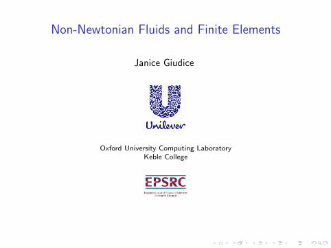
Extrusion of Paste

A soft, smooth, thick mixture of materials being forced through acylindrical chamber out of an exit nozzle. The material is tightlyconfined.

Multiple Extrusion of Pastes

Pastes with differing rheological properties layered undergoing thesame extrusion process with interfacial stability.

Complex Geometries: multiple nested chambers, the design of theextrusion chamber may be complex with internal moving parts andvarying nozzle geometry.

Multiple Extrusion of Pastes

Pastes with differing rheological properties layered undergoing thesame extrusion process with interfacial stability.

Complex Geometries: multiple nested chambers, the design of theextrusion chamber may be complex with internal moving parts andvarying nozzle geometry.

Non-Newtonian Fluids

Nonlinear stress tensor

T = −pI + k (x, |e(u)|) e(u)

I e(u) = 12

(∇u + (∇u)>

)is the rate of strain tensor.

I k (x, |e(u)|) is the apparent viscosity,

I | · | is the Frobenius norm.

Conservation of momentum and mass

ρ

„∂u

∂t+ (u · ∇) u

«= −∇p +∇ · (k (x, |e(u)|) e(u)) + f

∇ · u = 0

Non-Newtonian Fluids

Nonlinear stress tensor

T = −pI + k (x, |e(u)|) e(u)

I e(u) = 12

(∇u + (∇u)>

)is the rate of strain tensor.

I k (x, |e(u)|) is the apparent viscosity,

I | · | is the Frobenius norm.

Conservation of momentum and mass

ρ

„∂u

∂t+ (u · ∇) u

«= −∇p +∇ · (k (x, |e(u)|) e(u)) + f

∇ · u = 0

Simplifying the System

ρ

„∂u

∂t+ (u · ∇) u

«= −∇p +∇ · (k (x, |e(u)|) e(u)) + f

∇ · u = 0

Assuming that the flow is tightly confined and slow, we can dropthe non-linear term and neglect inertial effects. Also, we assumesteady flow.

∂u

∂t+ (u · ∇) u = 0

Under such restrictions, the governing equations are

−∇ · (k (x, |e(u)|) e(u)) +∇p = f

∇ · u = 0

Simplifying the System

ρ

„∂u

∂t+ (u · ∇) u

«= −∇p +∇ · (k (x, |e(u)|) e(u)) + f

∇ · u = 0

Assuming that the flow is tightly confined and slow, we can dropthe non-linear term and neglect inertial effects. Also, we assumesteady flow.

∂u

∂t+ (u · ∇) u = 0

Under such restrictions, the governing equations are

−∇ · (k (x, |e(u)|) e(u)) +∇p = f

∇ · u = 0

Simplifying the System

ρ

„∂u

∂t+ (u · ∇) u

«= −∇p +∇ · (k (x, |e(u)|) e(u)) + f

∇ · u = 0

Assuming that the flow is tightly confined and slow, we can dropthe non-linear term and neglect inertial effects. Also, we assumesteady flow.

∂u

∂t+ (u · ∇) u = 0

Under such restrictions, the governing equations are

−∇ · (k (x, |e(u)|) e(u)) +∇p = f

∇ · u = 0

Choice of Constitutive Relation

Possible choices are:

I Stokes flow: k(|e(u)|) ≡ 1

I Power-law model: k(|e(u)|) = µ |e(u)|r−2 , 1 < r < ∞

I Carreau model:k(|e(u)|) = µ∞ + (µ0 − µ∞)(1 + λ |e(u)|2)(θ−2)/2,µ0 > µ∞ ≥ 0 , λ > 0, θ ∈ (0,∞)

The Case for Numerical Simulation

I Mathematically non-trivial problems can be contemplated

I Experiments involving complex industrial fluids and processescan be expensive and time consuming

The Case for Numerical Simulation

I Mathematically non-trivial problems can be contemplated

I Experiments involving complex industrial fluids and processescan be expensive and time consuming

What exactly is Numerical Approximation?

A two-stage process

I Discretize the PDEs on some grid using a convergentrepresentation of the solution

I Solve the discrete problem accurately and efficiently

Au = f

What exactly is Numerical Approximation?

A two-stage process

I Discretize the PDEs on some grid using a convergentrepresentation of the solution

I Solve the discrete problem accurately and efficiently

Au = f

Current Numerical Approximation Methods

Finite Difference Methods Derivatives approximated locally usingTaylor series expansions

Finite Element Methods A versatile method based on thevariational formulation

Finite Volume Methods A method suited to conservation equations

Spectral Methods Approximations to derivatives are global.

Outline of The Finite Element Method

Consider a much simplified problem;

−∇2u = f in Ω

u = 0 on ∂Ω

Multiply by test function v and integrate over Ω

−∫

Ω

(∇2u

)v dΩ =

∫Ω

fv dΩ ∀v ∈ V ,

−∫

Ω∇u · ∇v dΩ =

∫Ω

fv dΩ ∀v ∈ V ,

a (u, v) = (f, v) ∀v ∈ V .

Outline of The Finite Element Method

Consider a much simplified problem;

−∇2u = f in Ω

u = 0 on ∂Ω

Multiply by test function v and integrate over Ω

−∫

Ω

(∇2u

)v dΩ =

∫Ω

fv dΩ ∀v ∈ V ,

−∫

Ω∇u · ∇v dΩ =

∫Ω

fv dΩ ∀v ∈ V ,

a (u, v) = (f, v) ∀v ∈ V .

Outline of the Finite Element Method

The problem is now to find u in V such that

a (u, v) = (f, v)

holds for every v in V .

Let Vh be a finite-dimensional subspace of V , then we seek uh inVh such that

a (uh, vh) = (f, vh)

holds for every vh in Vh.

Outline of the Finite Element Method

The problem is now to find u in V such that

a (u, v) = (f, v)

holds for every v in V .

Let Vh be a finite-dimensional subspace of V , then we seek uh inVh such that

a (uh, vh) = (f, vh)

holds for every vh in Vh.

Outline of the Finite Element Method

We seek uh in Vh such that

a (uh, vh) = (f, vh) , ∀ vh ∈ Vh.

Let φ1, . . . , φn be a basis of Vh, then

uh =n∑

i=1

Uiφi

Then the problem can be expressed as

a

(n∑

i=1

Uiφi , φj

)= (f, φj) ∀ j = 1, . . . , n.

This is system of n equations in n unknowns; Au = f

Outline of the Finite Element Method

We seek uh in Vh such that

a (uh, vh) = (f, vh) , ∀ vh ∈ Vh.

Let φ1, . . . , φn be a basis of Vh, then

uh =n∑

i=1

Uiφi

Then the problem can be expressed as

a

(n∑

i=1

Uiφi , φj

)= (f, φj) ∀ j = 1, . . . , n.

This is system of n equations in n unknowns; Au = f

Variational Formulation of Governing PDEs

Find u ∈ V = [W1,r0 (Ω)]d and p ∈ Q = Lr′

0 (Ω) = Lr′(Ω)/R

a(u, v) + b(p, v) = (f, v) ∀v ∈ V

b(q, u) = 0 ∀q ∈ Q.

Here

a(u, v) =

ZΩ

k(x , |e(u)|)e(u) : e(v)dΩ

b(q, v) = −Z

Ω

(∇ · v)q dΩ.

Inf-sup condition [Amrouche & Girault (1990)]: ∃c0 > 0 s.t.

infq∈Q

supv∈V

b(q, v)

‖q‖Q‖v‖V≥ c0 ∀q ∈ Q.

Variational Formulation of Governing PDEs

Find u ∈ V = [W1,r0 (Ω)]d and p ∈ Q = Lr′

0 (Ω) = Lr′(Ω)/R

a(u, v) + b(p, v) = (f, v) ∀v ∈ V

b(q, u) = 0 ∀q ∈ Q.

Here

a(u, v) =

ZΩ

k(x , |e(u)|)e(u) : e(v)dΩ

b(q, v) = −Z

Ω

(∇ · v)q dΩ.

Inf-sup condition [Amrouche & Girault (1990)]: ∃c0 > 0 s.t.

infq∈Q

supv∈V

b(q, v)

‖q‖Q‖v‖V≥ c0 ∀q ∈ Q.

Variational Formulation of Governing PDEs

Find u ∈ V = [W1,r0 (Ω)]d and p ∈ Q = Lr′

0 (Ω) = Lr′(Ω)/R

a(u, v) + b(p, v) = (f, v) ∀v ∈ V

b(q, u) = 0 ∀q ∈ Q.

Here

a(u, v) =

ZΩ

k(x , |e(u)|)e(u) : e(v)dΩ

b(q, v) = −Z

Ω

(∇ · v)q dΩ.

Inf-sup condition [Amrouche & Girault (1990)]: ∃c0 > 0 s.t.

infq∈Q

supv∈V

b(q, v)

‖q‖Q‖v‖V≥ c0 ∀q ∈ Q.

Finite Element Approximation

Let Vh ⊂ V and Qh ⊂ Q be finite-dimensional spaces consisting of p.w.polynomial functions, defined on a triangulation Th = T of thecomputational domain Ω.

Find uh ∈ Vh and ph ∈ Qh such that

a(uh, vh) + b(ph, vh) = (f, vh) ∀vh ∈ Vh

b(qh, uh) = 0 ∀qh ∈ Qh.

Discrete inf-sup condition: there exists c0 > 0, s.t.

infqh∈Qh

supvh∈Vh

b(qh, vh)

‖qh‖Q‖vh‖V≥ c0 ∀qh ∈ Qh.

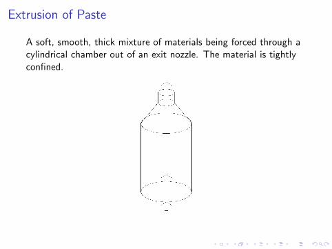
Finite Element Approximation

Let Vh ⊂ V and Qh ⊂ Q be finite-dimensional spaces consisting of p.w.polynomial functions, defined on a triangulation Th = T of thecomputational domain Ω.Find uh ∈ Vh and ph ∈ Qh such that

a(uh, vh) + b(ph, vh) = (f, vh) ∀vh ∈ Vh

b(qh, uh) = 0 ∀qh ∈ Qh.

Discrete inf-sup condition: there exists c0 > 0, s.t.

infqh∈Qh

supvh∈Vh

b(qh, vh)

‖qh‖Q‖vh‖V≥ c0 ∀qh ∈ Qh.

Finite Element Approximation

Let Vh ⊂ V and Qh ⊂ Q be finite-dimensional spaces consisting of p.w.polynomial functions, defined on a triangulation Th = T of thecomputational domain Ω.Find uh ∈ Vh and ph ∈ Qh such that

a(uh, vh) + b(ph, vh) = (f, vh) ∀vh ∈ Vh

b(qh, uh) = 0 ∀qh ∈ Qh.

Discrete inf-sup condition: there exists c0 > 0, s.t.

infqh∈Qh

supvh∈Vh

b(qh, vh)

‖qh‖Q‖vh‖V≥ c0 ∀qh ∈ Qh.

Some Preliminary Numerical Results

r = 2 r = 1 + 12 r = 1 + 1

4 r = 1 + 18 r = 1 + 1

16

What are we doing?

I Numerical simulation of incompressible, viscous extrusionflows for shear-thinning power-law fluids.

I Accurate capturing of the thin boundary layers in the flow.

I The accurate prediction of the free surface between twopastes with different rheological properties flowing in channelsor extruders.

Adaptive Finite Element Methods!!

SOLVE → ESTIMATE → MARK → REFINE

What are we doing?

I Numerical simulation of incompressible, viscous extrusionflows for shear-thinning power-law fluids.

I Accurate capturing of the thin boundary layers in the flow.

I The accurate prediction of the free surface between twopastes with different rheological properties flowing in channelsor extruders.

Adaptive Finite Element Methods!!

SOLVE → ESTIMATE → MARK → REFINE

What are we doing?

I Numerical simulation of incompressible, viscous extrusionflows for shear-thinning power-law fluids.

I Accurate capturing of the thin boundary layers in the flow.

I The accurate prediction of the free surface between twopastes with different rheological properties flowing in channelsor extruders.

Adaptive Finite Element Methods!!

SOLVE → ESTIMATE → MARK → REFINE

What are we doing?

I Numerical simulation of incompressible, viscous extrusionflows for shear-thinning power-law fluids.

I Accurate capturing of the thin boundary layers in the flow.

I The accurate prediction of the free surface between twopastes with different rheological properties flowing in channelsor extruders.

Adaptive Finite Element Methods!!

SOLVE → ESTIMATE → MARK → REFINE

What are we doing?

I Numerical simulation of incompressible, viscous extrusionflows for shear-thinning power-law fluids.

I Accurate capturing of the thin boundary layers in the flow.

I The accurate prediction of the free surface between twopastes with different rheological properties flowing in channelsor extruders.

Adaptive Finite Element Methods!!

SOLVE → ESTIMATE → MARK → REFINE

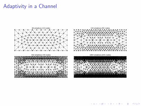
Adaptivity in a Channel

48 simplices;113 nodes 124 simplices;281 nodes

332 simplices;725 nodes 1064 simplices;2241 nodes

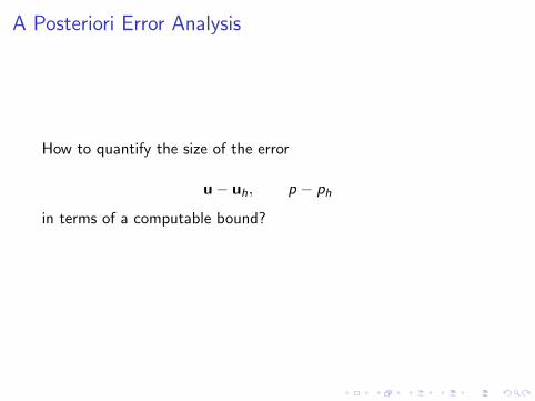
A Posteriori Error Analysis

How to quantify the size of the error

u− uh, p − ph

in terms of a computable bound?

A Posteriori Error Analysis

How to quantify the size of the error

u− uh, p − ph

in terms of a computable bound?

A posteriori error bound

Theorem. Let (u, p) ∈ V × Q denote the solution to b.v.p., and let(uh, ph) ∈ Vh × Qh denote its finite element approximation. Then, there is apositive constant C = C(K1, K2, c0, c

′0, r , ‖f‖V ′) s.t.

‖u− uh‖RV + ‖p − ph‖R

Q ≤ C“‖S1‖R′

V ′ + ‖S2‖R′

Q′

”,

where

R = maxr , 2, R = maxr ′, 2, 1/R + 1/R′ = 1, 1/R + 1/R′= 1,

and S1 and S2 residual functionals which are computably bounded.

[Barrett, Robson, Suli (2004)]

Some Numerical Results

r = 2

U V P

Some Numerical Results

r = 1.3

U V P

Some Numerical Results

r = 3.3

U V P

Some Numerical Results

r = 2 r = 1.3 r = 3.3

Conclusions, ongoing and future research

I We developed the a posteriori error analysis of finite elementapproximations to a class on non-Newtonian flows.

I Ongoing research: implementation into an adaptive finiteelement method in 2D.

I Future work: application to multiple fluids, time-dependentproblems in time-dependent geometries.