Embed Size (px)
Citation preview

Non-negatively constrained least squares and parameter choice by
the residual periodogram for the inversion of electrochemical
impedance spectroscopy
Jakob Hansena, Jarom Hoguea, Grant Sandera, Rosemary A Renauta,∗, Sudeep C Popatb
aSchool of Mathematical and Statistical Sciences, Arizona State University, Tempe, AZ 85287-1804, USAbSwette Center for Environmental Biotechnology, Biodesign Institute, Arizona State University, Tempe, AZ
85287, USA
Abstract
The inverse problem associated with electrochemical impedance spectroscopy requiringthe solution of a Fredholm integral equation of the first kind is considered. If the underlyingphysical model is not clearly determined, the inverse problem needs to be solved using aregularized linear least squares problem that is obtained from the discretization of the integralequation. For this system, it is shown that the model error can be made negligible by a changeof variables and by extending the effective range of quadrature. This change of variablesserves as a right preconditioner that significantly improves the condition of the system.Still, to obtain feasible solutions the additional constraint of non-negativity is required.Simulations with artificial, but realistic, data demonstrate that the use of non-negativelyconstrained least squares with a smoothing norm provides higher quality solutions thanthose obtained without the non-negative constraint. Using higher-order smoothing normsalso reduces the error in the solutions. The L-curve and residual periodogram parameterchoice criteria, which are used for parameter choice with regularized linear least squares, aresuccessfully adapted to be used for the non-negatively constrained problem. Although theseresults have been verified within the context of the analysis of electrochemical impedancespectroscopy, there is no reason to suppose that they would not be relevant within thebroader framework of solving Fredholm integral equations for other applications.
Keywords: Inverse problem, non-negative least squares, regularization, ill-posed, residualperiodogram2000 MSC: 65F10, 45B05, 65R32
1. Introduction
We consider the numerical solution of ill-posed inverse problems that are motivated bymeasurements of electrochemical impedance spectra from which a model of the underlying
∗Corresponding Author: Rosemary Renaut, 480 965 3795Email addresses: [email protected] (Jakob Hansen), [email protected] (Jarom Hogue),
[email protected] (Grant Sander), [email protected] (Rosemary A Renaut), [email protected] (Sudeep CPopat )
URL: math.asu.edu/~rosie (Rosemary A Renaut)
Preprint submitted to J Computational and Applied Mathematics June 1, 2014

physical reaction mechanisms is desired. There is extensive literature on a wide range of ap-plications in which the same, or similar models can be applied. These include measurementsfor solid oxide fuel cells [4, 14, 15, 16, 17, 19, 25, 26], microbial fuel cells [22], as well as ofphysiological parameters, and from a diverse range of dielectric models, [2, 18, 21, 28]. Inthese applications the unknown distribution function of relaxation times (DRT) is related toa set of impedance measurements by the Fredholm integral equation
Z(ω) = R0 +Rpol
∫ ∞0
g(t)
1 + iωtdt, (1.1)
where ω is angular frequency, t is time, and g(t) is the desired DRT with normalization∫∞0g(t)dt = 1.There are several models used to represent the individual processes of a DRT, many of
which are mostly used for the analysis of dielectric materials and are described in [2]. Severalare directly applicable to the fuel cell modeling case, where they usually take the form of theo-retical circuit components used in constructing equivalent circuit models. Equivalent circuitelements used for fuel cell modeling include the Cole-Cole (also known as RQ or ZARC)element, the Generalized Finite-Length Warburg element, and the Gerischer impedance[2, 13, 19]. In analysis of specific fuel cell designs a log-normal form for the DRT hasalso been used [21, 22]. Here we focus our investigations on the Cole-Cole DRT, whichcan be rendered temperature independent only in the limiting cases of β → 0, 1, and thetemperature independent lognormal DRT, denoted throughout by RQ and LN, respectively.
The RQ impedance is a generalization of a simple parallel RC circuit and for a singleprocess has an impedance given by
ZRQ(ω) =1
1 + (iωt0)β, (1.2)
where t0 is the point of maximum distribution, and β is a shape parameter controlling thewidth of the distribution. The corresponding DRT is
gRQ(t) =1
2πt
sin βπ
cosh(β ln
(tt0
))+ cos βπ
, (1.3)
which reduces to the Dirac delta distribution when β = 1, [2]. There is, however, no analyticform for the impedance corresponding to the log-normal DRT given by
gLN(t) =1
tσ√
2πexp
(−(ln(t)− µ)2
2σ2
). (1.4)
Although a number of options have been presented in the literature for geometricallyassessing the parameterization of the DRT from impedance data for a single physical process,e.g. as noted in [28], for given measured and noisy impedance data from multiple processesthere are effectively only two basic approaches that may be considered to estimate the DRT.When a specific analytic but parameter dependent form for the impedance is known, asin (1.2), parametric nonlinear least squares (NLS) fitting may be used to determine theunderlying parameters of the impedance and hence of the DRT, [18]. On the other hand,
2

when no analytic representation of the impedance is available, as in (1.4), it is still possible,but more computationally expensive, to apply a parametric nonlinear fit by using directnumerical integration of (1.1). In either case, an alternative is to apply a linear least squares(LLS) fit directly to the DRT, but this is also challenging due to the general ill-posednessof the problem, e.g. [3, 8, 10, 11, 27]. Both approaches, as well as the geometric analyses,have been extensively considered in the literature, e.g. [2]. When the model for the DRT isnot known, perhaps when the physical process is not completely understood or the numberof processes has not been determined, the only option is to fit directly to the DRT, withoutidentifying its specific parameterization.
Before further pursuing the LLS fit, we illustrate in Section 2 the use of direct NLSfitting for a simple one-process example in order to emphasize the (self-evident) significanceof the prior knowledge of the model. Assuming the wrong model leads to apparently robustdata fitting, while at the same time potentially leading to incorrect conclusions about theDRT parameterization. With this conclusion we move in Section 3 to an analysis of thesystem describing the LLS fitting that arises when approximating (1.1) discretely. Thedirect discretization of (1.1) leads to two ill-conditioned systems of equations, for the realand imaginary parts separately. Most literature on the problem suggests the use of LLSfor the systems obtained in this way, in conjunction with regularization to stabilize theestimation of the solution, [14, 29]. In contrast, it was suggested in [19], that rather thanestimating the DRT in the given t-space, a transformation to s−space via s = log(t) wouldbe preferable and that the resulting ill-posed system be solved using a non-negative leastsquares (NNLS) algorithm, specifically imposing the constraint that the DRT is a positivedistribution. In Section 3.2 we investigate the modeling error that arises when using thes−space transformation, leading to new results that quantify the total modeling error dueto discretization and truncation in (1.1) for both real and imaginary terms. The results gobeyond those presented in [22] for the t−space formulation, by providing error estimateswhich are primarily determined by the kernel h(ω, t) = (1 + iωt)−1, only relying on standardsmoothness and decay conditions for the DRT functions.
The numerical algorithms for the estimation of the DRT are discussed in Section 4. Firstit is demonstrated that the s−transformation serves as a right preconditioner, leading tomore stable estimation of the underlying basis for the solution when the time discretizationis chosen appropriately in relation to the frequency measurements. A brief and standardoverview of Tikhonov regularization for the solution of LLS is given in Section 4.3, with par-ticular focus on the estimation of the regularization parameter. This discussion leads to newregularization parameter estimation techniques for the NNLS problem. In particular, theL-curve (LC) and residual periodogram (RP) parameter estimation techniques are extendedto the NNLS algorithm, with minimal additional algorithmic development, Section 4.4. Fi-nally, the theoretical developments are verified and evaluated for a set of impedance datasets,consisting of two and three physical processes, which are motivated by examples that areseen from practical configurations. The presented results justify both the use of inclusionof the non-negativity (NN) constraint for finding approximate DRTs from multiple physicalprocesses, and the use of the RP and LC for estimating the regularization parameter withinthis context. The latter is of more general use for ill-posed systems of linear equations withNN constraints. Conclusions of the work are provided in Section 6.
3

2. Parametric NLS Fitting: Distinguishing between models for one process
We investigate parametric nonlinear fitting to impedance data given by (1.1) with R0 = 0and Rpol = 1 (without any loss of generality). For a given DRT, simulated data forZ = Z1 − iZ2 were generated for realistic frequencies ω ∈ [10−2, 105] sampled logarith-mically at 65 points, providing the exact fitting vector [Z1;Z2] of length 130. The exactdata were generated for the RQ and LN DRTs, (1.3) and (1.4), respectively, with pa-rameters t0 = 0.1, β = 0.7203 and σ = ln(2.3) chosen to provide DRTs aligned with re-spect to the location and height of the peak in the s = ln(t/t0) space, see Figure 1(b),β = (2/π) arctan ((
√2π/σ) exp(−σ2/2)), see Section 3.1 and [7]. For the RQ impedance
(1.2) was used to provide the vector Z, whilst for the LN impedance the data were gener-ated by Matlab’s integrate() function with the bounds 0 and Inf. The resulting Nyquistplots (complex plot of Z) and components Z1 and Z2 are quite similar, see Figures 1(c)-1(e),and identification of the underlying model from such data, particularly when contaminatedby noise, may not be possible.
10−2
10−1
100
101
0
1
2
3
4
5
6
7
8
LN
RQ
(a) DRTs: t−space
−5 0 50
0.5
1
1.5
2
2.5
3
3.5
LN
RQ
(b) DRTs: s−space
0.1 0.2 0.3 0.4 0.5 0.6 0.7 0.8 0.9
0.05
0.1
0.15
0.2
0.25
0.3
0.35
LN
RQ
(c) Nyquist plot
10−2
100
102
104
10−8
10−6
10−4
10−2
LN
RQ
(d) Components Z1
10−2
100
102
104
10−4
10−3
10−2
10−1
LN
RQ
(e) Components Z2
Figure 1: Simulated exact data measured at 65 logarithmically spaced points in ω. In each case the solidline indicates the RQ functions and the � symbols the LN functions.
To simulate noisy measurements, white noise at a level ηj was added according to
Zij = Z + ηjei, (2.1)
where Zij denotes the noisy data, and the vector ei is the ith column of the array of size130 × 50 generated using the Matlab function randn, corresponding to 50 realizations ofwhite noise, for noise levels ηj j = 1 : 21 logarithmically spaced between 10−6 and 10−2.5.The choice of the highest noise level used here was determined by comparing the obtainedvalues for Z as compared to data seen in practice. The lowest noise level corresponds toeffectively noise-free data, but avoids the inverse crime by assuring that the data used inthe inversion were not exactly prescribed by the underlying forward model. Nonlinear fittingwas performed using the Matlab function lsqcurvefit() initialized with β = 0.8, σ = ln(2),and t0 = 1/ω0, where ω0 is obtained as the argument of the dominant peak value in Z2, asis commonly used to find the value t0 [2]. Bounds 0 < t0 < 100, and 0.1 < β, σ < 1 wereimposed. Further, scaling of each DRT was introduced through a parameter α satisfying0 < α < 1.1 initialized with α = 1.
Two fittings were performed for each Zij, one assuming the correct DRT and one assumingthe incorrect DRT, i.e. given Z generated for the RQ DRT a fit was perfumed assumingthe correct RQ impedance and the incorrect LN impedance values. Similarly for the LNimpedance values, correct fitting was performed by fitting with a LN DRT, and incorrect
4

fitting by an RQ DRT. When using the RQ DRT for fitting the analytic form of the impedancewas used, whilst for the LN DRT all calculations used the Matlab integrate() function.Hence for each noise level and realization four fitting pairs were considered, RQ to RQ, LNto RQ, LN to LN, and RQ to LN. For fixed noise level ηj and each fitting pair the meanand variance of the residual calculated over the 50 realizations was calculated. Figure 2demonstrates the imperfect residuals over all noise levels for the mismatched fitting, and theincreasing, but relatively smaller, residuals for the matched fittings. Further, fitting to theLN by RQ yields a smaller residual than fitting RQ by LN. In Figure 2 the 95% confidencebounds determined by the variance of the residual are very tight, indicating the robustnessof the process.
10−6
10−5
10−4
10−3
10−10
10−8
10−6
10−4
10−2
100
Mean Fit by RQ
Upper 95% bound
Lower 95% bound
Mean Fit by LN
Upper 95% bound
Lower 95% bound
(a) Fitting to the RQ
10−6
10−5
10−4
10−3
10−10
10−8
10−6
10−4
10−2
100
Mean Fit by RQ
Upper 95% bound
Lower 95% bound
Mean Fit by LN
Upper 95% bound
Lower 95% bound
(b) Fitting to the LN
Figure 2: Residual norms fitting one process to the impedance spectrum of a DRT consisting of one processwith white noise in subfigure 2(a) the RQ process and in subfigure 2(b) the LN process.
To obtain a clearer picture of the quality of the fit, the mean and standard deviationin the estimates for the underlying parameters for three different noise levels are given inTables 1-2. In each case the matched fitting does a good job of parameter estimation for allnoise levels, while the mismatched fitting is consistently wrong. Fitting the RQ impedancewith the assumption of a LN DRT generates data that suggests the peak position has movedto the left, and the peak is relatively higher, Figure 3(a). Fitting the LN impedance by a RQDRT generates a fit moved to the right with the height quite well-preserved, Figure 3(b).However, the processes are still aligned in the s = log(t/t0) space, Figures 3(c)-3(d), eachplotted with respect to the identified t0.
10−2
10−1
100
101
0
1
2
3
4
5
6
7
8
LN
RQ
(a) RQ (1.3) by LN (1.4)
10−2
10−1
100
101
0
1
2
3
4
5
6
7
8
LN
RQ
(b) LN (1.4) by RQ (1.3)
−5 0 50
1
2
3
4
5
6
7
8
LNfit
RQ
(c) RQ by LN: s−space
−5 0 50
0.5
1
1.5
2
2.5
3
3.5
LN
RQfit
(d) LN by RQ: s−space
Figure 3: Fitting functions with the consistent mean values obtained and reported in Tables 1-2. In Figures3(a) and 3(c) fitting the RQ with the LN, and in Figures 3(b)-3(d) fitting the LN with the RQ.
We conclude that if the information on the underlying DRT is not known, fitting based
5

on the parameters of the DRT itself will lead to misleading interpretation of the results.Consequently, LLS fitting which simply finds an estimate for the DRT, without finding itsparameterization, is the only feasible option for understanding the physical processes whenthe precise model has not been determined. We also observe that the fitting as seen in thes−space is much more informative in detecting differences and similarities of the DRTs. Ofcourse these results are for the case of a single process. In practice multiple processes aregenerally exhibited and the impedance fitting is then also less robust in separating the linearcombinations, even when the model is predetermined.
Noise level ηFit Parameter True 1e− 6 5.6e− 5 3.2e− 3
RQ to RQ β 0.72 0.72(5e− 07) 0.72(3e− 05) 0.72(1e− 03)RQ to RQ t0 0.10 0.10(1e− 07) 0.10(6e− 06) 0.10(4e− 04)RQ to RQ α 1.00 1.00(3e− 07) 1.00(1e− 05) 1.00(8e− 04)
LN to RQ σ 0.83 1.00(8e− 16) 1.00(3e− 14) 1.00(5e− 09)LN to RQ t0 0.10 0.03(4e− 08) 0.03(2e− 06) 0.03(1e− 04)LN to RQ α 1.00 0.97(2e− 07) 0.97(1e− 05) 0.97(7e− 04)
Table 1: Mean and standard deviation of absolute errors for obtained parameters for fitting to the RQ DRT.
Noise level ηFit Parameter True 1e− 6 5.6e− 5 3.2e− 3
RQ to LN β 0.72 0.86(4e− 07) 0.86(2e− 05) 0.86(1e− 03)RQ to LN t0 0.10 0.20(2e− 07) 0.20(1e− 05) 0.20(6e− 04)RQ to LN α 1.00 1.01(3e− 07) 1.01(1e− 05) 1.01(8e− 04)
LN to LN σ 0.83 0.83(2e− 06) 0.83(1e− 04) 0.83(5e− 03)LN to LN t0 0.10 0.10(3e− 07) 0.10(2e− 05) 0.10(9e− 04)LN to LN α 1.00 1.00(2e− 07) 1.00(1e− 05) 1.00(8e− 04)
Table 2: Mean and standard deviation of absolute errors for obtained parameters for fitting to the LN DRT.
3. Nonparametric Linear Least-Squares
3.1. Numerical Quadrature
When a model for the physical system has not been established, a nonparametric methodof estimating its DRT must be used. The most straightforward method of discretization,discussed at length in [22] with respect to the introduced model error, uses the trapezoidalrule for quadrature with logarithmically spaced points in time to generate matrices A1 andA2 approximating the real and imaginary integral operators h(ω, t) = h1(ω, t) − ih2(ω, t)in (1.1). In [19] it was suggested to use a change of variables for the integration before
6

obtaining the quadrature formulae but no discussion or analysis of the potential advantagesor disadvantages was provided. Let s = ln t, then
Z(ω) =
∫ ∞0
h(ω, t)g(t) dt =
∫ ∞−∞
h(ω, es)f(s) ds, f(s) := tg(t). (3.1)
For the DRTs (1.3)-(1.4) we obtain the functions
fRQ(s) =1
2π
sin(βπ)
(cosh(β(s− ln(t0))) + cos(βπ))(3.2)
fLN(s) =1
σ√
2πexp
(−(s− µ)2
2σ2
), ln(t0) = µ− σ2, (3.3)
A motivation for this change of variables is to improve the interpretation of the graph of thefunction when plotted on the linear scale for s as compared to the logarithmic scale for t,see e.g. Figure 1(b).
In [22, (8)-(10)] formulae for the trapezoidal quadrature weights an in∫ ∞0
h(ω, t)g(t) dt ≈∫ Tmax
Tmin
h(ω, t)g(t) dt ≈N∑n=1
anh(ω, tn)g(tn), (3.4)
show that an are dependent on the logarithmic spacing for t, tn+1−tn = (∆t)n+1 = tn(10∆t−1), where ∆t is constant.1 The same rule applied for the integral with respect to the svariable, chosen so that tn = esn , gives constant ∆s = sn+1 − sn = ln(tn+1) − ln(tn) =ln(10)∆t. With the standard notation that the double prime on the summation indicatesthat first and last terms are halved, this yields, with s1 = smin = ln (Tmin) and sN = smax =ln (Tmax) ∫ ∞
−∞h(ω, es)f(s) ds ≈
∫ smax
smin
h(ω, es)f(s) ds ≈ ∆sN∑n=1
′′h(ω, esn)f(sn). (3.5)
It is of interest to further investigate the impact of this change of variables on the con-dition of the resulting systems of equations and on the modeling error obtained from (3.5)so as to justify the use of the s−space formulation rather than the t−space formulation.This follows the similar investigation that was presented in [22] for (3.4). The discretizationrequires the choice of values for Tmin and Tmax, as well as the number of points N used in thediscretization of f(s) or g(t). Since in this problem t and ω have a reciprocal relationship,as noted in, e.g., [14, 25], we will assume the range for t is reciprocal to the given range forω, i.e., Tmax = 1/ωmin and Tmin = 1/ωmax. Forthwith we will use s1 and sN to denote smin
and smax, and we reiterate that N depends on the number of samples for the impedance.
3.2. Model error
The model error involved in the discretization of the integral operators stems from twosources: the truncation of the improper integral and the approximation of the integral bya finite quadrature rule. It will be shown here that the model error can be reduced to anegligible level given reasonable assumptions on the DRT.
1We note the error in [22] which gives these in terms of log rather than ln.
7

3.2.1. Quadrature error
Bounds for the quadrature error for the logarithmically-spaced trapezium rule (3.4) ap-plied for the lognormal g(t) (1.4) were shown in [22, (23)]. Because of the use of the variablespacing the error bound for each term of the quadrature varies with tn, and thus a rapidlydecreasing integrand as t → ∞ is necessary in order to control the error. It is well-knownthat the quadrature error for the standard constant spacing composite trapezium rule isgiven by, where we use H(s) = h(ω, es)f(s) and |H ′′(ζn)| := maxs∈[sn,sn+1] |H ′′(s)|,
|Equad| ≤N−1∑n=1
|H ′′(ζn)|(∆s)3
12=
(∆s)3
12
N−1∑n=1
|H ′′(ζn)| = (sN − s1)3
12N2|H ′′(ζ)| (3.6)
for some ζ ∈ [s1, sN ] := Is, assuming appropriate continuity of H(s) on Is [1].
10−2
100
102
104
10−8
10−6
10−4
10−2
h1 (s)
h2 (s)
h1 (t)
h2 (t)
(a) RQ: t0 = 0.01, β = 0.5.
10−2
100
102
104
10−8
10−6
10−4
10−2
h1 (s)
h2 (s)
h1 (t)
h2 (t)
(b) RQ: t0 = 0.1, β = 0.5.
10−2
100
102
104
10−8
10−7
10−6
10−5
10−4
10−3
10−2
h1 (s)
h2 (s)
h1 (t)
h2 (t)
(c) RQ: t0 = 1.0, β = 0.5.
Figure 4: Quadrature error for a single RQ process with N = 65 for quadrature in s and t as a functionof ω, plotted on a log-log scale, for the kernels corresponding to the real and imaginary components of theimpedance.
10−2
100
102
104
10−15
10−10
10−5
100
h1 (s)
h2 (s)
h1 (t)
h2 (t)
(a) LN: t0 = 0.01, σ = ln(3).
10−2
100
102
104
10−15
10−10
10−5
100
h1 (s)
h2 (s)
h1 (t)
h2 (t)
(b) LN: t0 = 0.1, σ = ln(3).
10−2
100
102
104
10−20
10−15
10−10
10−5
100
h1 (s)
h2 (s)
h1 (t)
h2 (t)
(c) LN: t0 = 1.0, σ = ln(3).
Figure 5: Quadrature error for a single LN process with N = 65 for quadrature in s and t as a functionof ω, plotted on a log-log scale, for the kernels corresponding to the real and imaginary components of theimpedance.
Figures 4-5 contrast the quadrature error as a function of ω using N = 65 for (3.4) and(3.5), the t and s integrals, respectively, for the two DRTs (1.3)-(1.4). To obtain the error, anestimate of the true integral (to machine epsilon) was calculated using the Matlab function
8

integral(). For each formulation of the DRT, the errors were estimated for a single processfor three choices of t0, and a fixed spreading parameter, β = 0.5 and σ = ln(3), respectively.The quadrature error for the integration evaluated with respect to s is so small as to benegligible for this problem; the error is always less than 10−4 and 10−5, for the RQ and LNcases, respectively, and always far less than the error obtained for quadrature applied to theintegration with respect to the variable t. We note further that for any integrand which hassimilar decay properties on the interval, the same results will apply.
3.2.2. Improved Quadrature
Although we have shown that the error is small, the quadrature (3.5) can be furtherimproved as an approximation to the improper integral in (3.5). It was noted in [14] thatthe quadrature can be improved for the case of kernel h2 by extrapolating the data outsidethe given interval by a straight line. Because the composite trapezium rule is based onlinear interpolation on each interval, it is immediately possible to extend the range of theintegration by an interval ∆s, or indeed on any arbitrary interval, on either side by anextrapolation that assumes H(sN + ∆s) = H(s1 −∆s) = 0, leading to the modification∫ ∞
−∞h(ω, es)f(s) ds ≈
∫ sN+∆s
s1−∆s
h(ω, es)f(s) ds ≈ ∆sN∑n=1
h(ω, esn)f(sn). (3.7)
Here the only change is that the weight on the first and last terms is no longer halved.This extends the finite range for the quadrature, but does not handle the entire truncation.Suppose now that f(s) > 0 and lims→±∞ f(s) = 0, then analytic integration gives∫ ∞
sN
f(s)hk(ω, es) ds ≤ f(sN)
∫ ∞sN
hk(ω, es) ds = f(sN)rk,N(ω, esN ), (3.8)
rk,N(ω, esN ) :=
{12
ln(1 + (ωesN )−2) k = 1π2− tan−1(ωesN )) k = 2,
(3.9)
while ∫ s1
−∞f(s)h2(ω, es) ds ≤ f(s1)
∫ s1
−∞h2(ω, es) ds = f(s1)r2,1(ω, es1) (3.10)
r2,1(ω, es1) := tan−1(ωes1). (3.11)
For the real kernel at the left hand end, separating out the kernel integration in the sameway is not useful. Instead we must use again the assumption that f(s) decays fast enoughthat f(s1 −∆s) = 0, (or equivalently that the entire integrand decays fast enough), and setr1,1(ω, es1) = 1
2∆s h1(ω, es1). Putting these results together leads to the modified quadrature
rule which more accurately accounts for the integration outside the range determined by Is,∫ ∞−∞
hk(ω, es)f(s) ds ≈ ∆s
N∑n=1
′′hk(ω, esn)f(sn) + f(sN)rk,N(ω, esN ) + f(s1)rk,1(ω, es1).
(3.12)
We emphasize the dependence here on the kernel of the integrand in obtaining this result,demonstrating the relative independence of the result on a sufficiently smooth DRT.
9

3.2.3. Truncation and Quadrature Error
The accuracy of (3.12) as an approximation to the improper integral in (3.5) depends onthe quadrature error (3.6) and the truncation error
ek(ω) =
∣∣∣∣∫ s1
−∞hk(ω, s)f(s) ds+
∫ ∞sN
hk(ω, s)f(s) ds− f(s1)rk,1(ω, s1)− f(sN)rk,N(ω, sN)
∣∣∣∣ .Let IL = [−∞, s1], and IR = [sN ,∞], and assume that Is has been chosen appropriately forthe given data, so that f(s) is monotonically decreasing on both IL and IR, i.e. there existsε > 0 such that |f(s)| ≤ ε, s ∈ IL ∪ IR. Then considering first k = 2
e2(ω) ≤(
maxs∈IL|f(s)− f(s1)| r2,1(ω, es1)
)+
(maxs∈IR|f(s)− f(sN)| r2,N(ω, esN )
)≤ ε (r2,1(ω, es1) + r2,N(ω, esN )) = ε(
π
2+ tan−1(ωes1)− tan−1(ωesN )) ≤ επ
providing the total error for kernel h2
E2(ω) ≤ επ +(sN − s1)3
12N2|H ′′2 (ζ)|. (3.13)
For k = 1
e1(ω) ≤(∫ s1
−∞h1(ω, es) f(s) ds− ∆s
2h1(ω, es1)f(s1)
)+
(f(sN)
1
2ln(1 + (ωesN )−2)
).
For the first term observe h1(ω, es) < 1 for s ∈ IL and that the trapezoidal error bound can
be applied. Then, assuming∫ s1−∆s
−∞ f(s) ≤ δ(f), and using ζ ∈ [s1 −∆s, s1], we obtain∫ s1
−∞h1(ω, es)f(s) ds− ∆s
2h1(ω, es1)f(s1) ≤ (∆s)3
12|H ′′1 (ζ)|+ ∆s
2f(s1 −∆s) + δ(f),
and
e1(ω) ≤ (∆s)3
12|H ′′1 (ζ)|+ ∆s
2ε+ δ(f) + (
ε
2ln(1 + (ωesN )−2))
≤ ε
2(∆s+ ln(2)) +
(∆s)3
12H ′′1 (ζ) + δ(f),
where we use ωesN = ω/ω1. Therefore, now with ζ ∈ IL
E1(ω) ≤ ε
2(∆s+ ln(2)) + δ(f) +
(sN − s1)3
12N3(N + 1)|H ′′1 (ζ)|. (3.14)
In contrast to (3.13) this bound depends explicitly on the truncation error δ(f). On the otherhand, for practical N and Is, (∆s+ ln(2)) < 2π. The two bounds are thus very similar, bothdepending on the interval Is, and the smoothness of the integrand.
This analysis which examines the quadrature and truncation error together, contraststhe approach in [22] which found the bounds for each error separately, based explicitly on
10
the use of gLN(t). The same approach can be applied to examine the truncation error forgRQ(t), and is presented in Appendix A. In particular the bound for δ(f), which explicitlydepends on f , is provided by (A.4) for fRQ while the equivalent result for fLN can be foundin [22]. We deduce that the total model errors in (3.13)-(3.14) may be assumed small for thestandard DRTs which decay quickly away from their centers at t0 and have sufficiently smallsecond derivatives. Moreover, these bounds improve on those in [22] through the use of theimproved quadrature in s to take account of the extended range, thus reducing the size ofthe error introduced by truncating the improper integral. Further, these results are largelyindependent of the specific DRT, for any DRT satisfying reasonable decay and smoothnessassumptions in s−space.
4. Numerical Algorithms
We now turn to the numerical solution of the ill-posed system of equations defined by(3.12). In the subsequent discussion, matrices created from the original formulation of theproblem will be referred to without superscripts, while those created with the change ofvariable have a superscript s.
4.1. Right Preconditioning
Suppose that the measurements for the impedance are represented by the components ofvector b and that the unknowns f(sn) are components of the vector x1. Then the matrixequation, Asx1 ≈ b, for x1 is obtained from (3.5) with As
mn = ∆s′′h(ωm, e
sn), with the doubleprime indicating the halving for n = 1 and n = N . With the improved quadrature indicatedin (3.12) the components in As
mn are modified accordingly. In comparison, the discretizationfor g(tn) = f(sn)/tn is given by Ax ≈ b where x has components of g(t) and diag(t)x = x1.Contrasting these two formulations we see that the change of variables is effectively a rightpreconditioning of the original system: A diag(1./t)x1 = b. However, A diag(1./t) 6= As.The entries in each column differ in that the weights an in (3.4) after division by tn areproportional to sinh(∆s), excepting scale factors for n = 1 and n = N , as compared to ∆sfor matrix As. When ∆s is small, for large enough N , however, ∆s ≈ sinh(∆s), so thatthe two matrices are nearly equal [7]. We have already shown that the change of variablesimpacts the modeling error, we now consider its impact as a right preconditioner on thestability of the underlying system matrices.
4.2. Conditioning
The stability of the solution of a system of linear equations Ax ≈ b is well understood,see e.g. [3, 6, 8]. Given the singular value decomposition (SVD), A = UΣV T , the naıvesolution is x = V Σ−1UTb =
∑Ni=1 (uTi b)/σivi, where ui and vi are the ith columns of U
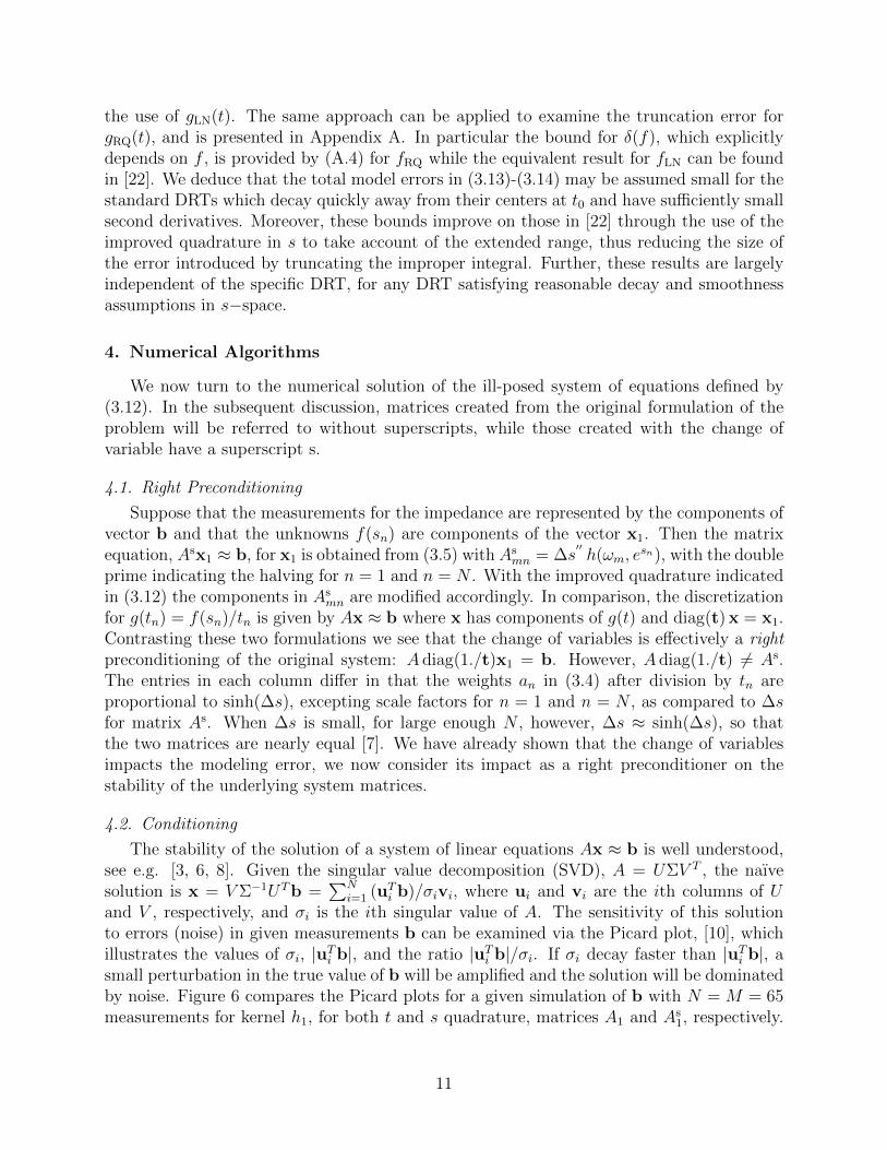
and V , respectively, and σi is the ith singular value of A. The sensitivity of this solutionto errors (noise) in given measurements b can be examined via the Picard plot, [10], whichillustrates the values of σi, |uTi b|, and the ratio |uTi b|/σi. If σi decay faster than |uTi b|, asmall perturbation in the true value of b will be amplified and the solution will be dominatedby noise. Figure 6 compares the Picard plots for a given simulation of b with N = M = 65measurements for kernel h1, for both t and s quadrature, matrices A1 and As
1, respectively.
11

10 20 30 40 50 60
10−10
10−5
100
σi
|ui
Tb|
|ui
Tb|/σ
i
(a) Picard plot A1x ≈ b1
10 20 30 40 50 60
10−8
10−6
10−4
10−2
100
σi
|ui
Tb|
|ui
Tb|/σ
i
(b) Picard plot As1x ≈ b1
Figure 6: Rght hand side b generated with a single RQ process with t0 = 10−2 and β = 0.8, using N = 65and ω logarithmically spaced on the interval [1e− 2, 1e+ 5].
For A1, |uTi b|/σi grow beginning at i = 1, while for As1 they only begin to grow consistently
around i = 28.The sensitivity shown in Figure 6 can be exposed in part by examining the condition
number, cond(A), independent of the measurement b. A more informative analysis, however,considers not only the condition but also its impact on the calculation of the basis vectorsfor the solution formed from the columns of the SVD matrices U and V . It can be shown,e.g. [11], that these columns predominantly approximate single frequency components. Thisfrequency content can be visualized by forming the normalized cumulative periodogram(NCP) for the vector regarded as a discrete time sampling of a continuous function, asexplained in the context of examining the residual vector in [9, 24] and the basis vectors in[22]. Vectors which are primarily contaminated by noise have an NCP which falls withinKolmogorov-Smirnov bounds for a chosen confidence level, [5]. Figure 7 contrasts the NCPsof the matrices A1 and As
1, illustrating the better separation of the frequency content for thebasis vectors formed from matrices U and V for matrix As
1. This suggests greater confidencein the use of a higher number of basis terms in the solution with the right preconditionedmatrix. A similar conclusion follows when comparing the matrices for the kernel h2.
Further demonstration of the impact of the right preconditioning is provided in Table 3which gives the condition of matrices for the t and s quadrature, for a selection of choicesfor It = [Tmin, Tmax] with N = 65. It is clear that the choice for It, and hence Is, has a largeimpact on the conditioning of the problem. For instance, if the range for t is too wide, thematrices will have several nearly linearly dependent columns, which greatly increases thecondition number of the matrix, and increases the dimension of the numerical null space.Likewise, if the range for t is too narrow, there will be nearly linearly dependent rows, againincreasing the condition number of the matrix. When the reciprocal relationship t = 1/ω isused to pick the sampling in t the optimal condition is obtained in both cases, as shown bythe bold face row of the table.
In general there are relatively few measurements of the impedance for the particularbiofuel application that can be used to find the solution. Typically there are on the orderof N = 65 usable values for each of Z1 and Z2, after estimates for the resistances Rpol andR0 in (1.1) have been found. It was shown in [22] that in order to make use of all available
12

0 5 10 15 20 25 30
0 5 10 15 20 25 30
(a) A1: U above and V below.
0 5 10 15 20 25 30
0 5 10 15 20 25 30
(b) As1: U above and V below.
Figure 7: Normalized Cumulative Periodograms and Kolmogorov-Smirnov 95% confidence bounds for whitenoise for the matrices A1 and As
1. The NCPs for A2 and As2 show a similar separation of the frequency
content of the respective basis vectors.
data, it is generally desirable to combine the matrices A1 and A2 into the stacked matrixA3 = [A1;A2] of size 2N × N , hence using systems associated with both kernels. Further,the overdetermined system can be replaced by a system using a square matrix A4 of size2N × 2N through increasing the sampling used in the quadrature for the kernel equations,hence providing increased resolution in the discretization of the solution vector. The sameapproach can be used for the s−quadrature matrices As
1 and As2 yielding matrices As
3 andAs
4. In practice, therefore, it is the impact of the scaling on these augmented matrices whichis also significant.
The results in Table 3 are given for the scaled matrices calculated using (3.5). To seethat the improvement in the quadrature has little impact on the overall conditioning, thecondition numbers of the matrices A1 to A4 for various quadrature rules, as noted by therespective equation numbers, are also shown in Table 4. Overall, the right preconditionedmatrices, regardless of selection of the system, exhibit better but still not ideal conditioning,so that the problem remains ill-posed and the solution is subject to noise-contamination.
13

Tmin Tmax A1 A2 As1 As
2
1e− 61e+ 1 9.70e+ 17 6.28e+ 18 2.83e+ 17 1.90e+ 171e+ 2 6.47e+ 17 1.05e+ 20 2.99e+ 17 2.41e+ 171e+ 3 4.73e+ 18 7.45e+ 19 4.58e+ 20 6.22e+ 18
1e− 51e+ 1 2.06e+ 19 1.74e+ 18 8.17e+ 17 6.40e+ 171e + 2 1.94e + 13 1.78e + 13 2.94e + 09 7.43e + 071e+ 3 2.20e+ 18 3.64e+ 19 2.12e+ 20 1.87e+ 18
1e− 41e+ 1 5.05e+ 21 1.55e+ 20 4.38e+ 19 2.44e+ 181e+ 2 1.52e+ 21 1.99e+ 18 1.09e+ 20 3.90e+ 181e+ 3 6.49e+ 19 6.98e+ 18 1.30e+ 21 1.41e+ 20
Table 3: Condition numbers for matrices A1, A2, As1, and As
2 for It = [Tmin, Tmax] and ω logarithmicallyspaced on the interval [1e− 2, 1e+ 5].
Quad Equation A1 A2 A3 A4
t (3.4) 1.5e+ 13 1.4e+ 13 7.5e+ 12 4.1e+ 20s (3.5) 2.9e+ 09 7.4e+ 07 4.6e+ 08 2.3e+ 18s (3.7) 3.1e+ 09 7.9e+ 07 5.0e+ 08 9.1e+ 17s (3.12) 2.8e+ 09 7.4e+ 07 4.6e+ 08 9.0e+ 18
Table 4: Comparing condition number of matrices with different quadratures for the optimal selection ofthe nodes for tn, using t = 1/ω. In this case, as compared to Table 3 the matrices are also reduced to sizeN = 64, consistent with the loss of data when estimating R0 and Rpol in (1.1).
4.3. Regularization
Given the ill-conditioning of the system matrices, regularization is required in order toselect an acceptable solution which provides a reasonable fit to the measured data, but is atthe same time controlled in its growth with respect to a chosen norm. There is an extensiveliterature discussing multiple formulations, e.g. [8, 10, 11, 12, 27] and for problems of thistype, Tikhonov regularization is frequently applied e.g. [14, 22, 29]. The solution is thenrecast as the solution of the regularized problem
x = arg min{‖Ax− b‖2 + λ2‖Lx‖2}, (4.1)
where λ is a parameter affecting the amount of regularization applied and L is a matrixchosen so the growth of x is controlled relative to the L−weighted norm. Typical choicesfor L are approximations to derivative operators of order 0, 1, or 2. For small problems theλ-dependent solution of (4.1) can be expressed in terms of the SVD, (L = I), or generalizedsingular value decomposition (GSVD), for other noninvertible choics for L, e.g. [8].
The choice of the regularization parameter λ is a nontrivial but well-studied problem.There are many algorithms available to choose this parameter. In general, these can bedivided into two categories: those which require some knowledge of the characteristics andmagnitude of the noise present in the right hand side, and those which do not. Techniquessuch as the discrepancy principle [8], the unbiased predictive risk estimator (UPRE) [27] andthe χ2 method [20] fall in the first category, while more heuristic methods such as the LC
14

criterion, the quasi-optimality criterion, and generalized cross-validation (GCV) fall in thesecond, [10]. The NCP criterion applied to the residual for the data fit, which is based onwork in [23] and then extended in [9, 24], falls between these two categories. It requires thatthe noise be white, or can be whitened, but does not require an estimate of its magnitude.
The LC criterion is commonly used when no information on the noise distribution isavailable. It relies on the fact that when plotted on a logarithmic scale, the weighted norm‖Lx‖ and the data fidelity norm ‖Ax − b‖ tend to form an L-shaped curve. That is, fora value of λ near the corner, an increase in λ would tend to increase the residual normwithout reducing the solution norm much, while a decrease in λ would increase the solutionnorm without much reducing the residual norm. The SVD and GSVD allow the simpleconstruction of the L-curve, and the corner is generally determined by finding the point ofmaximum curvature, as implemented in [10].
The NCP approach is based on the assumption that for an appropriately chosen λ thenoise in the measurements is transferred to the residual vector so that it is completelydominated by white noise. By calculating the NCP of the residual for suitably selectedvalues of λ, the smallest value which produces a residual vector reasonably approximatingwhite noise may be found. A common statistical test for white noise uses the Kolmogorov-Smirnov statistic to compare the residual NCP with the cumulative distribution function ofa uniform distribution. This test is described in more detail in, e.g., [5].
4.4. Non-negative Least-Squares
It was suggested in [19] that the solution of the DRT problem should use the additionalinformation on the DRT, namely that g(t) (and its cousin f(s)) are distribution functionssatisfying g(t) ≥ 0 for all t. Augmenting (4.1) by this constraint, yields the NNLS formulation
x = arg min{||Ax− b||2 + λ2||Lx||2, s.t. x ≥ 0}, (4.2)
for which efficient algorithms are available, given a specific choice for λ, including for instancethe algorithm in [12], which is implemented in Matlab. On the other hand, because we cannotimmediately express the solution in terms of an expansion, many common parameter choicemethods, such as the GCV and UPRE, are less feasible for finding a suitable λ. For thissmall problem, N ≈ 65, we explore the use of the two parameter choice methods, the LCcriterion and the NCP analysis of the residual vector.
For both methods, a standard approach for finding the optimal regularization parametercan still be applied. Specifically, solutions of (4.2) can be found for a range of values for λ,and the LC or NCP, respectively, applied to assess the quality of each solution, as brieflydescribed for (4.1) in Section 4.3. This contrasts with the parameter choice method presentedin [19] that relies on a specific implementation of the NNLS algorithm.
5. Simulation Results
The performance of the algorithms discussed and analyzed in Section 3 is investigatedfor simulated data sets exhibiting properties seen in practical situations. The data sets aredescribed first in Section 5.1. For each data set extensive comparisons have been performedusing both matrices A3 and A4, in order to assess whether the better conditioning of A3 or the
15

better resolution offered by A4 prevails as the optimum in each case. These examinationshave demonstrated that the additional resolution of A4 outweighs its worse conditioningas compared to A3, (see Table 3). While in many cases the results using A3 are quitecomparable, as noise increases systems solved with matrix A4 often provide better results.Thus in the presented results here we emphasize the comparisons between the LLS and NNLSmethods and do not give results for systems with matrix A3. Further results substantiatingthese comments are given in the supplementary materials [7].
5.1. Data sets
The parameters for the simulated data sets are detailed in Table 5. Simulations Aand B assume the existence of two underlying physical processes in the data; C assumesthree processes. The RQ model uses the parameters t0 and β, and the LN model uses theparameters µ = ln(t0) and σ. In each case the multiple processes are weighted by the weightsα. Note that the choice using µ = ln(t0) for the LN process provides data which are centeredat t0 in the s−space, and as can be seen in Figures 8(b), (g) and (l), are approximateltyaligned with the RQ model data. The set of figures for each simulation A to C demonstratesthe similarity of the chosen RQ and LN data, indicating the difficulty of distinguishingbetween these models from the impedance data alone, Figures 8(c)-(e), (h)-(j) and (m)-(o).In all plots, other than the Nyquist, the y-data are plotted against x on a logarithmic scale.
Parameters t0 β σ α
Simulation A [10−3.5, 100.5] [0.8, 0.8] [ln(2), ln(2)] [0.5, 0.5]Simulation B [10−1.5, 10−0.5] [0.7, 0.8] [ln(2.4), ln(2)] [0.35, 0.65]Simulation C [10−3, 1, 10] [0.8, 0.7, 0.7] [ln(2), ln(2.1), ln(2.2)] [0.6, 0.2, 0.2]
Table 5: Simulation parameters for simulated test data
The two processes in simulation Set A have peaks that are far enough apart that theindividuals processes are effectively separated. In such cases distinct peaks are seen in theplot of Z2(ω) at ω values which correspond to the reciprocals of the peak values in t. Suchinformation can be used to verify the results of the fitting by examining the locations of theresulting peaks, [7]. Moreover, this is therefore a relatively well-behaved situation for whichit should be possible to separate the underlying processes from measured data. In contrast,the two processes in set B are close but the existence of two peaks is not clear from Z2. Forthe three processes in set C the first is distinct in time from the latter two, which are closeand overlapping for larger time. Again the impedance data does not clearly indicate thenumber of processes in the data.
For testing the algorithms noise was added to the simulated values for Z following (2.1)as discussed in Section 2 for the examination of the NLS fitting. In all cases the data aresampled at 65 points logarithmically spaced on [ωmin, ωmax] = [10−2, 105], consistent withpractical data, and with sampling of the DRT at t = 1/ω yielding the equal spacing ins−space at 130 points for matrix A4. For the results presented here, the noise level η = 10−3
corresponding to .1% noise was chosen. Further results in [7] use noise levels 1% and 5%.While the higher noise levels, particularly around 1% may be more consistent with practicaldata, the actual noise level for the measured data is unknown. On the other hand, even withthe lower noise level the benefit of using the NNLS will become clear in Sections 5.2-5.3.
16

10−4
10−2
100
102
100
200
300
400
500
600
700
800
900
1000
1100
LN
RQ
(a) A: g(t)
10−4
10−2
100
102
0.05
0.1
0.15
0.2
0.25
LN
RQ
(b) tg(t)
0.1 0.2 0.3 0.4 0.5 0.6 0.7 0.8 0.9
0.02
0.04
0.06
0.08
0.1
0.12
0.14
0.16
0.18
0.2
LN
RQ
(c) Nyquist
10−2
100
102
104
0.1
0.2
0.3
0.4
0.5
0.6
0.7
0.8
0.9
LN
RQ
(d) Z1(ω)
10−2
100
102
104
0.02
0.04
0.06
0.08
0.1
0.12
0.14
0.16
0.18
0.2
LN
RQ
(e) Z2(ω)
10−4
10−2
100
102
5
10
15
20
25
30
35
LN
RQ
(f) B: g(t)
10−4
10−2
100
102
0.05
0.1
0.15
0.2
0.25
0.3
0.35
LN
RQ
(g) tg(t)
0.1 0.2 0.3 0.4 0.5 0.6 0.7 0.8 0.9
0.05
0.1
0.15
0.2
0.25
0.3
LN
RQ
(h) Nyquist
10−2
100
102
104
0.1
0.2
0.3
0.4
0.5
0.6
0.7
0.8
0.9
LN
RQ
(i) Z1(ω)
10−2
100
102
104
0.05
0.1
0.15
0.2
0.25
0.3
LN
RQ
(j) Z2(ω)
10−4
10−2
100
102
50
100
150
200
250
300
350
400
LN
RQ
(k) C: g(t)
10−4
10−2
100
102
0.05
0.1
0.15
0.2
0.25
0.3
LN
RQ
(l) tg(t)
0.1 0.2 0.3 0.4 0.5 0.6 0.7 0.8 0.9
0.05
0.1
0.15
0.2
0.25
LN
RQ
(m) Nyquist
10−2
100
102
104
0.1
0.2
0.3
0.4
0.5
0.6
0.7
0.8
0.9
LN
RQ
(n) Z1(ω)
10−2
100
102
104
0.05
0.1
0.15
0.2
0.25
LN
RQ
(o) Z2(ω)
Figure 8: Visualization of the simulation sets in Table 5, simulations A to C in subfigures (a)-(e), (f)-(j) and(k)-(m), respectively. In each plot the RQ simulation is illustrated with the solid line and the LN simulationwith the �. Except for the Nyquist plot, the scale of the x− axis is logarithmic.
5.2. Parameter Choice Methods
The NCP or residual periodogram (RP) was presented in [9, 23, 24] as a parameter choicemethod for the Tikhonov LLS problem (4.1). The use of the NCP applied to the residualfor finding the optimal parameter for the NNLS problem in (4.2) is, however, to the best ofour knowledge novel. We therefore first contrast the use of the LC and NCP for parameterchoice in the context of the NNLS constrained problem, with the three standard choices ofzero (L = I), first (L = L1) and second order (L = L2) derivative operators. These canbe obtained using the function get l in the Regularization toolbox [10]. The LC is alsoimplemented in the Regularization toolbox, while for the NCP we use the modification ofthe ncp in the toolbox, as used also for examining the frequency content of the basis vectorsas shown in Section 4.3. For both the NCP and L-Curve methods, solutions were found for50 choices of λ logarithmically spaced between 10−3.5 and 101.5. The optimal λ for the LCwas chosen using the corner of the LC, while for the NCP method, the Kolmogorov-Smirnovconfidence level for white noise uses p = 0.2. Each simulation was tested over 50 realizationsof .1% white noise.
For each noise realization the following information was recorded: the optimal solutionobtained by the NCP and LC parameter choice methods, with the optimally found λNCP
and λLC, and the optimal solution over all 50 choices for λ, with the respective λopt, asmeasured with respect to the absolute error in the s−space. The geometric means of λNCP
and λLC were calculated over all 50 noise realizations. The absolute error for each choice of
17

λ was also recorded for each noise realization, and the mean of these absolute errors takento give an average error for a given λ which can be visualized against λ. This follows theanalysis presented in [19] for the examination of the optimal regularization parameter. Inthe plots we thus show the average error against λ indicated by the ◦ plot. On the same plotwe indicate by the vertical lines the minimum λopt, and the geometric means for λNCP andλLC, as the solid (red), dashed (green) and dot-dashed ◦ (blue) vertical lines, respectively.For each simulation set the same procedure was performed for all smoothing norms L. Todemonstrate the dependence of the obtained solution on the optimal parameter, an examplerepresentative noise realization was chosen in each case and the solutions found using thechosen optimal parameters were compared with the exact solution. These are indicated bythe solid line (black), � (red) , × (green) and ◦ (blue), for the exact, λopt, λNCP, and λLC
solutions, respectively.The results are illustrated in Figures 9-14. Figures (a)-(c) in each case indicate the mean
error results for the different smoothing norms, and (d)-(f) demonstrate the sensitivity, orlack thereof, of the solution to the choice of λ near the optimum. We see that the resultsare remarkably consistent; the results with the identity weighted norm are generally lessrobust, while overall the NCP parameter choice marginally outperforms the LC. On theother hand, we also conclude that the use of either parameter choice method is robust interms of representing the optimal but practically unknown solution. Thus the NCP is tobe preferred for finding a suitable regularization parameter, and the L1 operator providesa compromise between over smoothing (a reduced peak) by L2 and under smoothing byL = I. Additional results for higher noise levels are provided in [7]. There it is shown thatfor noise levels at 5% the results deteriorate significantly in terms of the ability to accuratelydetermine the number of processes, that the LC results are significantly under smoothed andthat the extra resolution of matrix A4 is most obviously worthwhile, a result that is not atall clear by examination of the relative error. Overall, it is also clear that the LN processesare better resolved than those given by the RQ. This is not surprising given the graph of theRQ DRT for small t, see e.g. Figure 1(a), 3(a).
5.3. Comparison of LLS and NNLS
Finally we present a comparison of the NNLS results with those that are obtained usingthe Tikhonov regularization (4.1) for the same two parameter choice methods in order toassess whether the extra cost of the NN constraint is necessary. While extensive resultswere given in [22] for (4.1), these were only for the t−quadrature matrices. The results forthe A3 matrix and other noise levels are given in [7], where comparative tables of relativeerrors are also given. Here we present the results visually in Figures 15-20 equivalent to theNNLS results in Section 5.2. We see again that we cannot always anticipate for the optimumchoice of λ chosen by a specific algorithm will provide a solution with the minimum error, asmeasured by sampling over multiple choices for the regularization parameter. On the otherhand, the performance of these two parameter choice methods for the LS problem is goodevidence that the performance for the NNLS problem is consistent. For the solutions it isevident that NNLS provides better control of oscillations around zero due to the positivityconstraint. Moreover, because the NNLS does not need to control these oscillations, solutionsare less smooth and provide better resolution of the peaks. Given the sample sizes for theparticular microbial fuel cell application, and possibly other electrochemical applications
18

10−3
10−2
10−1
100
101
0
0.1
0.2
0.3
0.4
0.5
0.6
0.7
0.8
0.9
1
(a) L = I
10−3
10−2
10−1
100
101
0
0.1
0.2
0.3
0.4
0.5
0.6
0.7
0.8
0.9
1
(b) L = L1
10−3
10−2
10−1
100
101
0
0.1
0.2
0.3
0.4
0.5
0.6
0.7
0.8
0.9
1
(c) L = L2
10−5
10−4
10−3
10−2
10−1
100
101
102
0
0.05
0.1
0.15
0.2
(d) L = I
10−5
10−4
10−3
10−2
10−1
100
101
102
0
0.05
0.1
0.15
0.2
(e) L = L1
10−5
10−4
10−3
10−2
10−1
100
101
102
0
0.05
0.1
0.15
0.2
(f) L = L2
Figure 9: Mean error and example NNLS solutions. .1% noise, RQ-A data set, matrix A4.
10−3
10−2
10−1
100
101
0
0.1
0.2
0.3
0.4
0.5
0.6
0.7
0.8
0.9
1
(a) L = I
10−3
10−2
10−1
100
101
0
0.1
0.2
0.3
0.4
0.5
0.6
0.7
0.8
0.9
1
(b) L = L1
10−3
10−2
10−1
100
101
0
0.1
0.2
0.3
0.4
0.5
0.6
0.7
0.8
0.9
1
(c) L = L2
10−5
10−4
10−3
10−2
10−1
100
101
102
0
0.05
0.1
0.15
0.2
0.25
0.3
(d) L = I
10−5
10−4
10−3
10−2
10−1
100
101
102
0
0.05
0.1
0.15
0.2
0.25
0.3
(e) L = L1
10−5
10−4
10−3
10−2
10−1
100
101
102
0
0.05
0.1
0.15
0.2
0.25
0.3
(f) L = L2
Figure 10: Mean error and example NNLS solutions. .1% noise, RQ-B data set, matrix A4.
with limited sampling, the extra minimal cost associated with finding NNLS solutions offerssignificantly improved results. Indeed for higher noise levels, the LLS solutions offer littlereliable information about the actual physical processes of the model.
19

10−3
10−2
10−1
100
101
0
0.1
0.2
0.3
0.4
0.5
0.6
0.7
0.8
0.9
1
(a) L = I
10−3
10−2
10−1
100
101
0
0.1
0.2
0.3
0.4
0.5
0.6
0.7
0.8
0.9
1
(b) L = L1
10−3
10−2
10−1
100
101
0
0.1
0.2
0.3
0.4
0.5
0.6
0.7
0.8
0.9
1
(c) L = L2
10−5
10−4
10−3
10−2
10−1
100
101
102
0
0.05
0.1
0.15
0.2
0.25
(d) L = I
10−5
10−4
10−3
10−2
10−1
100
101
102
0
0.05
0.1
0.15
0.2
0.25
(e) L = L1
10−5
10−4
10−3
10−2
10−1
100
101
102
0
0.05
0.1
0.15
0.2
0.25
(f) L = L2
Figure 11: Mean error and example NNLS solutions. .1% noise, RQ-C data set, matrix A4.
10−3
10−2
10−1
100
101
0
0.1
0.2
0.3
0.4
0.5
0.6
0.7
0.8
0.9
1
(a) L = I
10−3
10−2
10−1
100
101
0
0.1
0.2
0.3
0.4
0.5
0.6
0.7
0.8
0.9
1
(b) L = L1
10−3
10−2
10−1
100
101
0
0.1
0.2
0.3
0.4
0.5
0.6
0.7
0.8
0.9
1
(c) L = L2
10−5
10−4
10−3
10−2
10−1
100
101
102
0
0.05
0.1
0.15
0.2
0.25
(d) L = I
10−5
10−4
10−3
10−2
10−1
100
101
102
0
0.05
0.1
0.15
0.2
0.25
(e) L = L1
10−5
10−4
10−3
10−2
10−1
100
101
102
0
0.05
0.1
0.15
0.2
0.25
(f) L = L2
Figure 12: Mean error and example NNLS solutions. .1% noise, LN-A data set, matrix A4.
6. Conclusion
The inverse problem associated with impedance spectroscopy of fuel cells has been dis-cussed. Two models for the underlying distribution function of relaxation times have beenconsidered. If the model for the DRT is known to be log-normal or RQ, then nonlinearfitting of the data using the right model can be done very consistently, while trying to fit tothe wrong model consistently returns inaccurate results. Moreover, when the noise level is
20

10−3
10−2
10−1
100
101
0
0.1
0.2
0.3
0.4
0.5
0.6
0.7
0.8
0.9
1
(a) L = I
10−3
10−2
10−1
100
101
0
0.1
0.2
0.3
0.4
0.5
0.6
0.7
0.8
0.9
1
(b) L = L1
10−3
10−2
10−1
100
101
0
0.1
0.2
0.3
0.4
0.5
0.6
0.7
0.8
0.9
1
(c) L = L2
10−5
10−4
10−3
10−2
10−1
100
101
102
0
0.05
0.1
0.15
0.2
0.25
0.3
0.35
(d) L = I
10−5
10−4
10−3
10−2
10−1
100
101
102
0
0.05
0.1
0.15
0.2
0.25
0.3
0.35
(e) L = L1
10−5
10−4
10−3
10−2
10−1
100
101
102
0
0.05
0.1
0.15
0.2
0.25
0.3
0.35
(f) L = L2
Figure 13: Mean error and example NNLS solutions. .1% noise, LN-B data set, matrix A4.
10−3
10−2
10−1
100
101
0
0.1
0.2
0.3
0.4
0.5
0.6
0.7
0.8
0.9
1
(a) L = I
10−3
10−2
10−1
100
101
0
0.1
0.2
0.3
0.4
0.5
0.6
0.7
0.8
0.9
1
(b) L = L1
10−3
10−2
10−1
100
101
0
0.1
0.2
0.3
0.4
0.5
0.6
0.7
0.8
0.9
1
(c) L = L2
10−5
10−4
10−3
10−2
10−1
100
101
102
0
0.05
0.1
0.15
0.2
0.25
0.3
(d) L = I
10−5
10−4
10−3
10−2
10−1
100
101
102
0
0.05
0.1
0.15
0.2
0.25
0.3
(e) L = L1
10−5
10−4
10−3
10−2
10−1
100
101
102
0
0.05
0.1
0.15
0.2
0.25
0.3
(f) L = L2
Figure 14: Mean error and example NNLS solutions. .1% noise, LN-C data set, matrix A4.
high, distinguishing which model to use in NLS fitting becomes problematic and may yieldresults that do not accurately describe the data. If the physical model for the process isnot known, the inverse problem for estimating the DRT needs to be solved by finding asolution to the discrete linear system. For this system, it has been shown that the modelerror can be made negligible by a change of variables and by extending the effective rangeof quadrature. Moreover, the conditioning of the problem improves considerably when the
21

10−3
10−2
10−1
100
101
0
0.1
0.2
0.3
0.4
0.5
0.6
0.7
0.8
0.9
1
(a) L = I
10−3
10−2
10−1
100
101
0
0.1
0.2
0.3
0.4
0.5
0.6
0.7
0.8
0.9
1
(b) L = L1
10−3
10−2
10−1
100
101
0
0.1
0.2
0.3
0.4
0.5
0.6
0.7
0.8
0.9
1
(c) L = L2
10−5
10−4
10−3
10−2
10−1
100
101
102
0
0.05
0.1
0.15
0.2
(d) L = I
10−5
10−4
10−3
10−2
10−1
100
101
102
0
0.05
0.1
0.15
0.2
(e) L = L1
10−5
10−4
10−3
10−2
10−1
100
101
102
0
0.05
0.1
0.15
0.2
(f) L = L2
Figure 15: Mean error and example LLS solutions. .1% noise, RQ-A data set, matrix A4.
10−3
10−2
10−1
100
101
0
0.1
0.2
0.3
0.4
0.5
0.6
0.7
0.8
0.9
1
(a) L = I
10−3
10−2
10−1
100
101
0
0.1
0.2
0.3
0.4
0.5
0.6
0.7
0.8
0.9
1
(b) L = L1
10−3
10−2
10−1
100
101
0
0.1
0.2
0.3
0.4
0.5
0.6
0.7
0.8
0.9
1
(c) L = L2
10−5
10−4
10−3
10−2
10−1
100
101
102
0
0.05
0.1
0.15
0.2
0.25
0.3
(d) L = I
10−5
10−4
10−3
10−2
10−1
100
101
102
0
0.05
0.1
0.15
0.2
0.25
0.3
(e) L = L1
10−5
10−4
10−3
10−2
10−1
100
101
102
0
0.05
0.1
0.15
0.2
0.25
0.3
(f) L = L2
Figure 16: Mean error and example LLS solutions. .1% noise, RQ-B data set, matrix A4.
right-preconditioned matrices As are used.To obtain feasible solutions to the discrete linear systems additional constraints are re-
quired. Simulations with artificial, but realistic, data demonstrate that the use of NNLSwith a smoothing norm provides higher quality solutions than those obtained without theNN constraint. Using higher-order smoothing norms also reduces the error in the solutions.Moreover, the LC and NCP criteria are effective regularization parameter choice techniques
22

10−3
10−2
10−1
100
101
0
0.1
0.2
0.3
0.4
0.5
0.6
0.7
0.8
0.9
1
(a) L = I
10−3
10−2
10−1
100
101
0
0.1
0.2
0.3
0.4
0.5
0.6
0.7
0.8
0.9
1
(b) L = L1
10−3
10−2
10−1
100
101
0
0.1
0.2
0.3
0.4
0.5
0.6
0.7
0.8
0.9
1
(c) L = L2
10−5
10−4
10−3
10−2
10−1
100
101
102
0
0.05
0.1
0.15
0.2
0.25
(d) L = I
10−5
10−4
10−3
10−2
10−1
100
101
102
0
0.05
0.1
0.15
0.2
0.25
(e) L = L1
10−5
10−4
10−3
10−2
10−1
100
101
102
0
0.05
0.1
0.15
0.2
0.25
(f) L = L2
Figure 17: Mean error and example LLS solutions. .1% noise, RQ-C data set, matrix A4.
10−3
10−2
10−1
100
101
0
0.1
0.2
0.3
0.4
0.5
0.6
0.7
0.8
0.9
1
(a) L = I
10−3
10−2
10−1
100
101
0
0.1
0.2
0.3
0.4
0.5
0.6
0.7
0.8
0.9
1
(b) L = L1
10−3
10−2
10−1
100
101
0
0.1
0.2
0.3
0.4
0.5
0.6
0.7
0.8
0.9
1
(c) L = L2
10−5
10−4
10−3
10−2
10−1
100
101
102
0
0.05
0.1
0.15
0.2
0.25
(d) L = I
10−5
10−4
10−3
10−2
10−1
100
101
102
0
0.05
0.1
0.15
0.2
0.25
(e) L = L1
10−5
10−4
10−3
10−2
10−1
100
101
102
0
0.05
0.1
0.15
0.2
0.25
(f) L = L2
Figure 18: Mean error and example LLS solutions. .1% noise, LN-A data set, matrix A4.
in the context of the NNLS formulation. Indeed, the use of the NCP criterion for parameterchoice with the NN constraint is a novel development of more general use for NNLS in otherapplications.
Although these results have been verified within the context of the analysis of fuel cells,there is no reason to suppose that they would not be relevant within the broader frameworkof solving Fredholm integral equations for other applications.
23

10−3
10−2
10−1
100
101
0
0.1
0.2
0.3
0.4
0.5
0.6
0.7
0.8
0.9
1
(a) L = I
10−3
10−2
10−1
100
101
0
0.1
0.2
0.3
0.4
0.5
0.6
0.7
0.8
0.9
1
(b) L = L1
10−3
10−2
10−1
100
101
0
0.1
0.2
0.3
0.4
0.5
0.6
0.7
0.8
0.9
1
(c) L = L2
10−5
10−4
10−3
10−2
10−1
100
101
102
0
0.05
0.1
0.15
0.2
0.25
0.3
0.35
(d) L = I
10−5
10−4
10−3
10−2
10−1
100
101
102
0
0.05
0.1
0.15
0.2
0.25
0.3
0.35
(e) L = L1
10−5
10−4
10−3
10−2
10−1
100
101
102
0
0.05
0.1
0.15
0.2
0.25
0.3
0.35
(f) L = L2
Figure 19: Mean error and example LLS solutions. .1% noise, LN-B data set, matrix A4.
10−3
10−2
10−1
100
101
0
0.1
0.2
0.3
0.4
0.5
0.6
0.7
0.8
0.9
1
(a) L = I
10−3
10−2
10−1
100
101
0
0.1
0.2
0.3
0.4
0.5
0.6
0.7
0.8
0.9
1
(b) L = L1
10−3
10−2
10−1
100
101
0
0.1
0.2
0.3
0.4
0.5
0.6
0.7
0.8
0.9
1
(c) L = L2
10−5
10−4
10−3
10−2
10−1
100
101
102
0
0.05
0.1
0.15
0.2
0.25
0.3
(d) L = I
10−5
10−4
10−3
10−2
10−1
100
101
102
0
0.05
0.1
0.15
0.2
0.25
0.3
(e) L = L1
10−5
10−4
10−3
10−2
10−1
100
101
102
0
0.05
0.1
0.15
0.2
0.25
0.3
(f) L = L2
Figure 20: Mean error and example LLS solutions. .1% noise, LN-C data set, matrix A4.
7. Acknowledgements
Authors Hansen, Hogue and Sander were supported by NSF CSUMS grant DMS 0703587:“CSUMS: Undergraduate Research Experiences for Computational Math Sciences Majorsat ASU”. Renaut was supported by NSF MCTP grant DMS 1148771: “MCTP: Mathe-matics Mentoring Partnership Between Arizona State University and the Maricopa CountyCommunity College District”, NSF grant DMS 121655: “Novel Numerical Approximation
24

Techniques for Non-Standard Sampling Regimes”, and AFOSR grant 025717 “Developmentand Analysis of Non-Classical Numerical Approximation Methods”. Popat was supportedby ONR grant N000141210344: “Characterizing electron transport resistances from anode-respiring bacteria using electrochemical techniques”. All authors wish to thank ProfessorCesar Torres from Arizona State University for discussions concerning the EIS modeling.
Appendix A. Truncation error
In (3.4)-(3.5) the semi-infinite (infinite) integrals are necessarily truncated. An analysisof the impact of the truncation for the lognormal DRT was presented in [22]. Here weinvestigate the extension of this result for the RQ model. Consider the single RQ processgiven by (3.2). The error from the upper truncation of the integral of this distribution atsN is given by
Eutrunc(sN) =
∫ ∞sN
f(s) ds =1
2−
tan−1(
tan(πβ2
)tanh
(β(sN−ln(t0))
2
))πβ
. (A.1)
Thus, in order to have Eutrunc(sN) < δ, we must have
sN >2
βtanh−1
(tan(πβ2
(1− 2δ))
tan πβ2
)+ ln(t0). (A.2)
Similarly, because the error from the lower truncation is given by
Eltrunc(s1) =
∫ s1
−∞f(s) ds =
1
2+
tan−1(
tan(πβ2
)tanh
(β(s1−ln(t0))
2
))πβ
, (A.3)
keeping Eltrunc < δ requires
s1 < −2
βtanh−1
(tan(πβ2
(1− 2δ))
tan πβ2
)+ ln(t0). (A.4)
Note that these error bounds are symmetric for t0 = 1; then s1 = −sN , Eltrunc(s1) =
Eutrunc(sN). On the other hand, as t0 moves to the right or left of 1, the bounds for sN ,
s1 shift in tandem, and thus we obtain a requirement on the total range
Etrunc = Eutrunc + El
trunc < 2δ for sN − s1 >4
βtanh−1
(tan(πβ2
(1− 2δ))
tan πβ2
). (A.5)
Once Etrunc is bounded, Lemma 1 from [22] can be applied directly, without proof.
Lemma 1. Suppose that s1 and sN are such that the upper and lower truncation errors areeach less than δ, i.e.,
Eutrunc(sN) =
∫ ∞−∞
f(s) ds−∫ sN
−∞f(s) ds < δ andEl
trunc(s1) =
∫ ∞−∞
f(s) ds−∫ ∞s1
f(s) ds < δ.
25

Then
E1trunc(ω) =
∫ ∞−∞
f(s)
1 + ω2e2sds−
∫ sN
s1
f(s)
1 + ω2e2sds ≤ δ
(1 +
1
1 + ω2e2sN
)≤ 2δ
E2trunc(ω) =
∫ ∞−∞
ωe2sf(s)
1 + ω2e2sds−
∫ sN
s1
ωe2sf(s)
1 + ω2e2sds ≤ (E2)min + (E2)max < δ,
where
(E2)min =
∫ s1
−∞
ωesf(s)
1 + ω2e2sds ≤
{δ ωes1
1+ω2e2s1≤ δ
2ωes1 < 1
δ2
ωes1 ≥ 1
(E2)max =
∫ ∞sN
ωesf(s)
1 + ω2e2sds ≤
{δ ωesN
1+ω2e2sN≤ δ
2ωesN ≥ 1
δ2
ωesN < 1.
Observe here that for the standard choice s1 = ln(Tmin) and sN = ln(Tmax), with Tmin =1/ωmax and Tmax = 1/ωmin, then ωes1 < 1, ωesN > 1, and the bounds for E2 simplify asgiven. Provided that the range for the integration moves with the location of t0, either tothe right or left, (A.5), the error is controlled appropriately. If on the other hand we alwaysassume t0 = 1 and pick the range symmetrically with respect to 0, the error will depend onthe actual location of t0.
[1] K.E. Atkinson, An Introduction to Numerical Analysis, (2nd ed.), New York: JohnWiley & Sons,,1998, ISBN 978-0-471-50023-0.
[2] E. Barsukov, J.R. Macdonald, editors, Impedance Spectroscopy: Theory, Experiment,and Applications, John Wiley and Sons, Hoboken, New Jersey, United States, 2005.
[3] A. Bjorck, Numerical Methods for Least Squares Problems, Soc. for Ind. and Appl.Math., Philadelphia, PA, 1986.
[4] C. Endler, A. Leonide, A. Weber, F. Tietz, E. Ivers-Tiffee, Time-dependent electrodeperformance changes in intermediate temperature solid oxide fuel cells, J. of the Elec-trochem. Soc., 157, (2010), B292-B298.
[5] W.A. Fuller, Introduction to Statistical Time Series, Wiley series in probability andstatistics, second edition, Wiley Publications, New York, United States,1996.
[6] G. Golub, C. van Loan, Matrix Computations, Third Edition, John Hopkins UniversityPress, Baltimore, Maryland, 1996,
[7] J. Hansen, J. Hogue, G. Sander, R.A. Renaut, Non-negatively constrained least squaresand parameter choice by the residual periodogram for the inversion of electrochemicalimpedance spectroscopy: Supplementary Materials, http://math.la.asu.edu/~rosie/cv0806/node1.html, 2013.
[8] P.C. Hansen, Rank-deficient and discrete ill-posed problems: numerical aspects of lin-ear inversion, SIAM Series on Fundamentals of Alg, Soc. for Ind. and Appl. Math.,Philadelphia, PA, 1998.
26

[9] P.C. Hansen, M. Kilmer, R.H. Kjeldsen, Exploiting residual information in the param-eter choice for discrete ill-posed problems, BIT 46, (2006), 4159.
[10] P.C. Hansen, Regularization Tools Version 4.0 for Matlab 7.3, Numer. Alg, 46, (2007),189-194.
[11] P.C. Hansen, Discrete inverse problems: Insight and algorithms, SIAM Series on Fun-damentals of Alg , 7, Soc. for Ind. and Appl. Math., Philadelphia, PA, 2010.
[12] C.L. Lawson, R.J. Hansen, Solving Least Squares Problems, SIAM Classics in Appl.Math., Soc. for Ind. and Appl. Math., Philadelphia, PA, 1995.
[13] A. Leonide, SOFC Modelling and Parameter Identification by means of Impedance Spec-troscopy. KIT Scientific Publishing, 2010.
[14] A. Leonide, V. Sonn, A. Weber, E. Ivers-Tiffee, Evaluation and Modeling of the CellResistance in Anode-Supported Solid Oxide Fuel Cells, J. of the Electrochem. Soc. 155,(1), (2008), B36-B41.
[15] A. Leonide, B. Ruger, A. Weber, W.A. Meulenberg, E. Ivers-Tiffee, Impedance study ofalternative (La,Sr)FeO(3-delta) and (La,Sr)(Co,Fe)O(3-delta) MIEC cathode composi-tions, J. of the Electrochem. Soc., 57, (2010), B234-B239.
[16] B. Liu, H. Muroyama, T. Matsui, K. Tomida, T. Kabata, K. Eguchi, Analysis ofimpedance spectra for segmented-in-series tubular solid oxide fuel cells, J. of the Elec-trochem. Soc., 157, (2010), B1858-B1864.
[17] B. Liu, H. Muroyama, T. Matsui, K. Tomida, T. Kabata, K. Eguchi, Gas Transportimpedance in segmented-in-series tubular solid oxide fuel cell, J. of the Electrochem.Soc., 157, (2011), B215-B224.
[18] J.R. Macdonald, Exact and approximate nonlinear least-squares inversion of dielectricrelaxation spectra, J. of Chem. Phys., 102, 15, (1995), 102:15.
[19] J. Macutkevic, J. Banys, A. Matulis, Determination of the Distribution of the RelaxationTimes from Dielectric Spectra, Nonlinear Anal.: Modelling and Control, 9, (1), (2004),7588.
[20] J. Mead, R.A. Renaut, A Newton root-finding algorithm for estimating the regularizationparameter for solving ill-conditioned least squares problems, Inverse Problems, (2009),25(2).
[21] T. M. Nahir, E.F. Bowden, The distribution of standard rate constants for electron trans-fer between thiol-modified gold electrodes and adsorbed cytochrome c. J. of Electroanal.Chem., 410, 1, (1996), 9–13.
[22] R.A. Renaut, R. Baker, M. Horst, C. Johnson D. Nasir, Stability and error analysis ofthe polarization estimation inverse problem for microbial fuel cells, Inverse Probl., 29,(2013), 045006 (24pp), doi:10.1088/0266-5611/29/4/045006.
27

[23] B.W. Rust, Truncating the singular value decomposition for ill-posed problems, TechnicalReport NISTIR 6131,, National Institute of Standards and Technology, (1998), URL =http://math.nist.gov/ BRust/pubs/TruncSVD/MS-TruncSVD.ps.
[24] B.W. Rust, D.P. O’Leary, Residual periodograms for choosing regularization parametersfor ill-posed problems, Inverse Probl., 24, 3, 2008, 034005 - 034035.
[25] H. Schichlein, A.C. Muller, M. Voigts, A. Krugel, E. Ivers-Tiffee, Deconvolution ofelectrochemical impedance spectra for the identification of electrode reaction mechanismsin solid oxide fuel cells, J. of Appl. Electrochem., 32, (2002), 875-882.
[26] V. Sonn, A. Leonide, E. Ivers-Tiffee, Combined Deconvolution and CNLS Fitting Ap-proach Appl. on the Impedance Response of Technical Ni/8YSZ Cermet Electrodes, J.of the Electrochem. Soc., 155, (7) (2008), B675-B679.
[27] C.R. Vogel, Computational Methods for Inverse Problems, SIAM: Philadelphia, PA,2002.
[28] L.C. Ward, T. Essex, B.H. Cornish, Determination of Cole parameters in multiplefrequency bioelectrical impedance analysis using only the measurement of impedances,Physiol. Meas., 27, 9, (2006), 839-850.
[29] J. Weese, A reliable and fast method for the solution of Fredholm integral equations ofthe first kind based on Tikhonov regularization, Comput. Phys. Commun., 69, (1992),99-111.
28