Contents lists available at ScienceDirect

Signal Processing

Signal Processing 100 (2014) 42–50

0165-16http://d

n CorrE-m

fatemizmmaho

journal homepage: www.elsevier.com/locate/sigpro

Non-negative sparse decomposition based on constrainedsmoothed ℓ0 norm

M.R. Mohammadi a, E. Fatemizadeh a, M.H. Mahoor b,n

a Department of Electrical Engineering, Sharif University of Technology, Tehran, Iranb Department of Electrical and Computer Engineering, University of Denver, Co, USA

a r t i c l e i n f o

Article history:Received 3 August 2013Received in revised form9 January 2014Accepted 14 January 2014Available online 22 January 2014

Keywords:Underdetermined equation systemSparse decompositionConstrained smoothed L0 normSparse representation-based classificationFacial expression recognition

84/$ - see front matter Published by Elsevierx.doi.org/10.1016/j.sigpro.2014.01.010

esponding author.ail addresses: mrmohammadi@ee.sharif.eduadeh@sharif.edu (E. Fatemizadeh),or@du.edu (M.H. Mahoor).

a b s t r a c t

Sparse decomposition of a signal over an overcomplete dictionary has many applicationsincluding classification. One of the sparse solvers that has been proposed for finding thesparse solution of a spare decomposition problem (i.e., solving an underdeterminedsystem of equations) is based on the Smoothed L0 norm (SL0). In some applications suchas classification of visual data using sparse representation, the coefficients of the sparsesolution should be in a specified range (e.g., non-negative solution). This paper presentsa new approach based on the Constrained Smoothed L0 norm (CSL0) for solving sparsedecomposition problems with non-negative constraint. The performance of the newsparse approach is evaluated on both simulated and real data. For the simulated data, themean square error of the solution using the CSL0 is comparable to state-of-the-art sparsesolvers. For real data, facial expression recognition via sparse representation is studiedwhere the recognition rate using the CSL0 is better than other solver methods (inparticular is about 4% better than the SL0).

Published by Elsevier B.V.

1. Introduction

Sparse representation of a signal over an overcompletedictionary has received great attentions in recent yearsdue to many applications in different areas such as imagedenoising [1,2], image inpainting [3,4], image compression[5], prediction [6], compressed sensing [7], blind sourceseparation [8–10], and classification [11]. In these applica-tions, one of the main steps is to find the sparse solution ofthe desired underdetermined system of linear equations.Many sparse solvers [12–16] have been proposed toapproximately find the sparse solution. However, in someapplications the coefficients of the sparse solution shouldbe in a specified range (e.g., non-negative solution). An

B.V.

(M.R. Mohammadi),

example of this application is the classification of visualdata (facial expressions) using sparse representation. Thispaper proposes a fast and novel approach for sparsedecomposition with non-negative constraints.

A system of linear equations can be stated in matrixform as As¼ x, where xARn is the knowns vector, sARm isthe unknowns vector, and AARn�m is the coefficientsmatrix (aka, dictionary). If the number of unknowns (m)is larger than the number of equations (n), the system andthe dictionary are called underdetermined and overcom-plete, respectively. Thus, the number of solutions s thatsatisfy in As¼x can be more than one. Therefore, to chooseone of the solutions some extra constraints should beadded to the problem. One of the popular constraints is tohave the sparsest solution for the problem which can beformulated as

ℓ0 : s0 ¼ arg min‖s‖0 subject to As¼ x ð1Þwhere ‖ � ‖0 is the L0 norm counting the nonzero entries ofa vector. The optimization problem in (1) is very sensitive

M.R. Mohammadi et al. / Signal Processing 100 (2014) 42–50 43

because of the exact condition As¼x. To reduce thissensitivity and make the sparse representation robust, itis proposed in [17] to use the following more stableoptimization problem:

ℓ0s : s0 ¼ arg min‖s‖0 subject to ‖As�x‖2oε ð2Þ

where ε is an acceptable error that should be lower thanthe noise energy [17]. In other words, the solutionobtained using Eq. (2) is the sparsest solution in whichits error L2 norm is lower than ε. The cost function in boththe above optimization problems is the L0 norm of thesolution. However, L0 norm is neither continuous nordifferentiable, and solving the associated optimizationproblems requires a combinational search. Therefore, therewere proposed some well-known approaches to approx-imate the solution of them. The sparse coders will bereviewed in the next section.

In some applications such as classification via sparserepresentation, it is desired to apply some constraints (e.g.,non-negative constraint) on the coefficients of the sparsesolution. To apply any constraint on the coefficients of thesparse solution, the usual way is to add it to the aboveoptimization problems. For example, adding the non-negative constraint to the problem in (2) yields

ℓ0s;nn : s0 ¼ arg min‖s‖0 subject to ‖As�x‖2oε; 8 i siZ0

ð3ÞIn this paper, we propose a penalty method that

changes the cost function to apply any desired constrainton the coefficients of the sparse solution implicitly. Tooptimize this new optimization problem, we reformulatethe SL0 approach and optimize it in a coarse to finemanner.

The rest of the paper is organized as follows. The state-of-the-art sparse solvers are reviewed in Section 2. Theproposed algorithm for sparse decomposition with non-negative constraint is discussed in Section 3. In Section 4,the experimental results for simulated as well as real dataare reported. Finally, the paper is summarized in Section 5.

2. Sparse decomposition solvers

It is proven in [18] that minimizing L0 norm in Eqs. (1)–(3)is NP-hard. Hence, some alternative algorithms are pro-posed to approximate the sparse solution. The mostpopular sparse solver is Basis Pursuit (BP) [12] that triesto optimize L1 norm instead of L0 norm as stated below:

ℓ1s : s1 ¼ arg min‖s‖1 subject to ‖As�x‖2oε ð4ÞThe optimization problem of ℓ1 can easily be converted

to a linear and convex problem [12] and there are manytools to optimize them. Nevertheless, the essential ques-tion is the relationship between the solutions of ℓ1 and ℓ0.It is proven in [19] that if the number of non-zero elementsin the sparse solution is lower than a threshold (dependedon the correlation between the dictionary atoms), thesolutions of the ℓ1 and ℓ0 are exactly the same. In addition,this condition is sufficient but not necessary, and in somestudies such as [20] it is shown that without satisfying thiscondition, the ℓ1 can recover the sparse solution.

The non-negative version of the BP algorithm is pro-posed in [21] which solves the following problem:

ℓ1s;nn : s1 ¼ arg min‖s‖1 subject to ‖As�x‖2oε;

8 i siZ0 ð5Þ

The main drawback of the BP algorithm is its computa-tional cost that can be a bottleneck for large scale pro-blems. The Matching Pursuit (MP) algorithm [13] is a fastmethod for approximating the ℓ0 problem. The nature ofMP is greedy and it tries to optimize only one element ofthe sparse solution in each step. In other words, in the firststep the closest atom to the input vector x is selected andits corresponding coefficient is determined such that therepresentation error is minimum with only one non-zeroelement. In each of the next steps, the value of one furtherelement is optimized in a manner that the representationerror be minimized. In fact, in each step the value of oneelement in s is optimized until the representation error isless than a threshold or the number of non-zero elementsis more than a limit.

Compared to the BP method, the MP algorithm is veryfast because it requires just a simple search in each step.However, it is greedy and there is no guarantee that itsfinal solution is similar to the result of ℓ0. To improve theaccuracy of MP while maintaining its low complexity,some algorithms are proposed so that the most popularof them is Orthogonal MP (OMP) [15]. In the OMP, in eachstep after selecting the best atom, all of the previouscoefficients are ignored and the best representation (i.e.,the least square error) of x on the selected atoms arecomputed by a pseudo-inverse. The OMP is more accuratethan the MP, and it is shown in [22] that given certainconditions on the dictionary, OMP guarantees to find theoptimal solution. However, the condition of OMP is morestringent than BP to find the best solution, and its solutioncan be far from the sparse solution when the sparsity ofthe solution is low (we will discuss in the experimentalresults).

Non-negative variants of OMP proposed in severalworks such as [23,24], where all of them select themaximum correlation (instead of maximum absolute cor-relation), and use non-negative least square (NNLS)instead of least square.

Another interesting tool for sparse decomposition isbased on Smoothed L0 norm (SL0) presented in [14]. TheSL0 directly minimizes the L0 norm in a coarse to fineapproach. The main problem to optimize the ℓ0 is thediscontinuous nature of the L0 norm. The authors of [14]propose to optimize a smoothed version of L0 norm. Forinstance, f sðsÞ in (6) is a smoothed version of s0 (s power 0):

f s sð Þ ¼ 1�exp�s2

2s2

� �ð6Þ

where s is the controlling parameter for the smoothness off sðsÞ. Fig. 1 illustrates the s0 and f sðsÞ for some values of s.As can be observed, for large values of s, f sðsÞ is a verysmooth function and for small values of s, f sðsÞ converges tos0. In this way, FsðsÞ is defined in (7) as an approximation of

Fig. 1. s0 in comparison to its smoothed version for some values of s.

M.R. Mohammadi et al. / Signal Processing 100 (2014) 42–5044

L0 norm:

FsðsÞ ¼ ∑m

i ¼ 1f sðsiÞ � ‖s‖0 ð7Þ

and the new optimization problem is

s0 ¼ arg min FsðsÞ subject to As¼ x ð8ÞIt is shown in [14] that for sufficiently large values of s, thesolution of Eq. (8) is the least square solution of As¼x (i.e.,the solution given by the pseudo-inverse of A). However,the sparse solution is related to s¼0. Thus, it is proposed touse a coarse to fine approach that in the first iteration alarge value is selected for s. Then, in each iteration the valueof s is decreased and the solution of the previous step isused as the initialization value of s. The main advantage ofSL0 is in the fact that it tries to minimize an L0 normproblem instead solving alternative functions such as L1norm. In addition, it is shown in [14] that the SL0 is 2–3orders of magnitude faster than the state-of-the-artinterior-point linear programming solvers that typicallyused in the BP algorithm such as in [25]. However, it shouldbe noted that for large scale problems, some faster algo-rithms (such as in-crowd algorithm [26]) than interior-point methods exist for solving the BP.

3. Proposed algorithm

As mentioned in the previous section, one interestingsparse solver is based on SL0. The goal of this paper is todevelop a constrained version of SL0. One of the popularmethods to solve a constrained optimization problem inthe optimization context is the penalty method [27] whichreplaces the constrained optimization problem by a seriesof unconstrained problems whose solutions ideally con-verge to the solution of the original constrained problem.In this section, we adopt a penalty method to addconstraints to the SL0 approach. This approach is calledConstrained Smoothed L0 norm (CSL0). In this section, firstthe non-negative version of SL0 is introduced. Then, theapproach is generalized to other constraints.

3.1. Non-negative sparse decomposition

In the L0 norm, the sign of the coefficients does notmatter and only the number of non-zero coefficients isenumerated. Thus, to apply the non-negative constraint on

the coefficients of the sparse solution, it is possible tomodify L0 norm in order to the penalty of negativecoefficients be higher than the positive ones. The weighteds0 is defined in (10):

wk;1 sð Þ ¼ kþ12

� k�12

sign sð Þ� �

¼ k if so01 if s40

(ð9Þ

s0k;1 ¼ s0 �wk;1ðsÞ ð10Þ

where subscripts k, 1 express the weights of each arms ofs0k;1 (Fig. 2). Then, the weighted L0 norm is defined as asum of s0k;1 over all of the elements of s:

‖s‖k;10 9 ∑m

i ¼ 1s0i �wk;1ðsiÞ ð11Þ

Thus, the new optimization problem with the weighted L0norm is defined as

ℓ0k;1 : sk;1 ¼ arg min‖s‖k;10 subject to As¼ x ð12Þ

If the value of k is infinite in ℓ0k;1, the penalty for negative

coefficients is infinite and consequently any of the ele-ments in the final solution cannot be negative. However,similar to ℓ0, optimization of ℓ0

k;1 is NP-hard, and a sparsesolver should be developed. Moreover, if k is infinite, theoptimization of ℓ0

k;1 with any tool may be ill-conditioned.Thus, as a relaxed version, we design a limited value for kto obtain the non-negative constraint without the abovedifficulty.

Lemma 1. If x can be represented as a positive linearcombination of K atoms of A, the value of k should be greaterthan K in order to all of the coefficients of sk;1 be non-negative.

Proof. The cost value for the desired solution with Kpositive coefficients in ‖s‖k;10 is K. On the other hand, thepenalty for each negative coefficient is k. Thus, the costvalue of a solution that has only one negative value is k,and if this cost is more than the cost value of the desiredsolution, it can be found using (12). In other words, if k isgreater than K, all of the coefficients of sk;1 will be non-negative.Now, we reformulate the SL0 for non-negative sparse

decomposition. The smoothed version of the weighed‖s‖k;10 is depicted in Fig. 2. This function can be obtained

Fig. 2. Weighted s0 in comparison to its smoothed version for some values of s.

Table 1The pseudo-code of the proposed sparse solver with non-negativeconstraint based on CSL0

Inputs: A, xInitialization:(1) Choose the value of smin, K, L, μ, d, ε(2) s ¼AT ðAAT Þ�1x(3) s¼ 2 maxjsjWhile s4smin

(1) k¼ 1þK � smin=s(2) For l¼ 1 : L

(a) Compute ΔGs;kðsÞ using (15) and (16)(b) s’s�μ=k� ΔGs;kðsÞ(c) If ð‖As�x‖24εÞ

s’s�AT ðAAT Þ�1ðAs�xÞ(d) End If

(3) End For(4) s¼ s� dEnd WhileOutput: s

M.R. Mohammadi et al. / Signal Processing 100 (2014) 42–50 45

by multiplication of s0k;1 by smoothed s0 as

gs;kðsÞ ¼ s0k;1 � f sðsÞ ð13ÞGs;kðsÞ is defined as a sum of the gs;kðsÞ for all elements of s:

Gs;kðsÞ ¼ ∑m

i ¼ 1gs;kðsiÞ � ‖s‖k;10 ð14Þ

Gs;kðsÞ is called Constrained Smoothed L0 norm (CSL0)since its optimization with a consistent value of k mayresult in a sparse solution that its coefficients are con-strained to be non-negative. The minimization of Gs;kðsÞcan be performed in a coarse (large s) to fine (small s)approach. Since the first optimization problem (i.e., withlarge s) is convex, it has only one local minimum that canbe obtained using a simple optimization algorithm such asgradient descent. In the next iterations, the optimizationmay become non-convex but their initial point is obtainedfrom the previous optimization and can be close to thelocal minimum. Thus, in these iterations the gradientdescent algorithm can also be effective. The derivative ofgs;kðsÞ and the gradient of Gs;kðsÞ are computed as

∂gs;kðsÞ∂s

¼ ss2

exp�s2

2s2

� ��wk;l sð Þ ð15Þ

ΔGs;k sð Þ ¼ ∂gs;kðs1Þ∂s1

⋯∂gs;kðsnÞ

∂sn

� �Tð16Þ

However, the optimization problem is constraint to As¼x.Thus, it is possible to use gradient-projection algorithm forits optimization (i.e., after each iteration the solutionshould be projected to the feasible region that is As¼x).The projection of any s to the feasible region can beperformed with the below equation:

s’s�AT ðAAT Þ�1ðAs�xÞ ð17ÞTo make the proposed sparse solver robust to noise, weshould change the strict constraint As¼x to its relaxed‖As�x‖2oε. It is shown in [16] that to obtain thisrobustness for SL0, it is sufficient that the projection stepusing Eq. (17) performs only when the solution is outsideof the feasible region (i.e., ‖As�x‖2Zε). We use this ideato make the proposed CSL0 approach robust to noise.The pseudo-code of the proposed algorithm is presented

in Table 1. The following parameters are initialized in thefirst step: smin (the minimum value of s that should be avery small number), K (the maximum number of positive

coefficients in the desired solution), L (the number of itera-tions for decreasing s and minimizing Gs;kðsÞ), μ (the gradientdescent factor), d (the decreasing factor of s), ε (the acceptablereconstruction error), s (the initial solution that can beobtained using a pseudo-inverse which has the minimumL2 norm and corresponds to s¼1), and s (the initial value ofs that should be a large number). The initial value of s, basedon the theoretical discussions in [14], is chosen two times ofthe maximum absolute value of the initial s because in thiscase expð� s2i =2s

2Þ40:88 for all 1r irm, and this value of sacts virtually like infinity for all the values of si.After the initialization step, with two nested loops, Gs;kðsÞ is

minimized, s is decreased, and k is increased to obtain thenon-negative sparse solution. Since the initial s computed bya simple pseudo-inverse corresponds to s¼ inf and k¼1, wedecrease s to smin and increase k to Kþ1 slowly to form asmooth trajectory. This smooth trajectory prevents themethod from becoming stuck at a local minimum. Then, inthe inner loop the gradient-projection algorithm is used tooptimize Gs;kðsÞ with constraint ‖As�x‖2oε. After anyoptimization, s is decreased by factor d. □

3.2. Generalization to other constraints

The presented algorithm is proposed to apply non-negative constraint on the elements of the sparse solution.

Fig. 3. An example of simulated data with 40 positive coefficients (firstrow), the corresponding x vector (second row), and the solutions of theproposed CSL0 algorithm on the 0, 5 and final iterations.

M.R. Mohammadi et al. / Signal Processing 100 (2014) 42–5046

This algorithm can easily be generalized to other con-straints by changing w function in (9). If the desired rangefor the elements is from a to b, i.e., (a b), the generalizedweighted s0 can be defined as

wða;bÞk;1 sð Þ ¼ kþ1

2þ k�1

2sign s�að Þsign s�bð Þ

� �ð18Þ

Two special cases of this function correspond to theunconstrained and the non-negative constraint cases. Inthe unconstrained case, a and b are �1 and 1, respec-tively. Consequently, signðs�aÞ is 1, and signðs�bÞ is �1that result in wð�1;1Þ

k;1 ðsÞ ¼ 1. In the non-negative case, aand b are �1 and 0, respectively that result in wð�1;0Þ

k;1ðsÞ ¼ ððkþ1Þ=2�ððkþ1Þ=2ÞsignðsÞÞ which is exactly equalto (9).

By defining (18), it is possible to smooth wða;bÞk;1 ðsÞ in a

similar manner and obtain the sparse solution with thedesired constraint on its elements. Furthermore, it ispossible to choose different values of a and b for differentelements of the sparse solution to apply different con-straints on the elements of the sparse solution. Thus, thegeneralized weighted L0 norm is defined as

‖s‖k;1;ða;bÞ0 9 ∑m

i ¼ 1s0i �wðai ;biÞ

k;1 ðsiÞ ð19Þ

where ai and bi are two bounds of the desired range for theith element of s. Also, a and b are two vectors that specifythe desired range for all elements of the desired sparsesolution.

4. Experimental results

In this section the performance of the proposed algo-rithm is evaluated first on the simulated data and then in areal application (i.e., facial expression recognition). We usethe MATLAB implementation of the approach that can bedownload from http://ee.sharif.ir/�mrmohammadi/CSL0/CSL0.m.

4.1. Simulated data

In this experiment, we use a white zero-mean unit-variance Gaussian random process to generate atoms of arandom dictionary A with the size of 100�200. Then,some different ideal sparse vectors, s, with 1–100 positivecoefficients and unit L2 norm, are generated randomly. Togenerate these sparse vectors, we use an integer uniformrandom process to select the nonzero elements, andanother unit-variance uniform random process for theirvalues. For each solution, the vector x is computed byx¼As. Now, for each x the sparse solution of As¼x iscomputed using any of the sparse solvers and the meansquare error (MSE) is considered as the first performancemeasure:

MSE s; s� �¼ ‖s� s‖22

mð20Þ

where s and s are the ideal and the estimated sparsesolutions, respectively. As the second performance mea-sure, we compare the non-zero coefficients of s and s. Forthis, the number of locations of the first ‖s‖0 dominant

elements of s and s that are identical is enumerated andnormalized to ‖s‖0.

Fig. 3 illustrates an example of this procedure with theproposed CSL0 algorithm. In Fig. 3, a random vector s with40 positive coefficients and the corresponding x areplotted in the first and the second rows, respectively. Thesolutions of CSL0 after 0, 5 and final iterations are shownin the third to fifth rows, respectively. As can be observed,in the initial vector (i.e., the minimum L2 norm solution)most of the coefficients are non-zero and some of themnegative. In the next iterations, the solution is convergedto the desired solution and its final MSE is only 1.4e�8. Inthis experiment, we use the following parameters for theCSL0 algorithm: smin ¼ 10�10, K ¼ ‖s‖0, L¼5, μ¼2, d¼0.75,and ε¼10�2.

M.R. Mohammadi et al. / Signal Processing 100 (2014) 42–50 47

To compare the performance of the proposed algorithmwith the other sparse solvers, for each number of non-zeroelements (from 1 to 100), the algorithms are executed 100times and the average MSE of them is plotted in Fig. 4(a). Aswas expected, proper use of the priori information about thenon-negativity of the coefficients has led to a better accuracyof the non-negative versions of all sparse solvers (i.e., BP, OMPand SL0). When the number of non-zero elements is lowerthan 30, all the non-negative algorithms work properly. Byincreasing the number of non-zero coefficients, the perfor-mance of the NN-OMP is decreased dramatically since itsnature is greedy. The performance of the NN-BP is decreasedfrom k¼35 while the sparse solution is unique at least tillko50 (to study the uniqueness conditions of the sparsesolution, we refer readers to [28,29,23]). CSL0 works properlyfor a larger number of non-zero coefficients; however, whenk450 (i.e., the sparse solution cannot be unique), its accuracydecreases and becomes worse than the NN-BP for ‖s‖0Z58.

A similar behavior is observed for the percent of over-lapped non-zero coefficients shown in Fig. 4(b). CSL0works properly for a larger number of non-zero elementsthan other sparse solvers. However, for very large ‖s‖0, theNN-BP outperforms the CSL0.

4.2. Real data: facial expression recognition via sparserepresentation

One of the interesting applications of sparse decom-position is in pattern classification that has received greatattention in recent years [30,31]. In these classifiers, the

Fig. 4. Comparing the proposed CSL0 approach with state-of-the-artsparse solvers on the simulated data, (a) average MSE and (b) averagepercent of non-zero coefficients overlapped between the ideal and theestimate sparse solutions, for 100 runs versus the number of non-zerocoefficients.

feature vector of the test object is represented sparsely onan overcomplete dictionary, and the object is classifiedbased on the sparse solution. In this paper, the SparseRepresentation-based Classification (SRC) framework [11]is used for facial expression recognition. In SRC, all of thetraining feature vectors are used as the atoms of adictionary as

A¼ ½v1;1 v1;2 ⋯ v1;n1 ⋯ vc;1 ⋯ vc;nc � ð21Þ

where vi;j is the jth training feature vector of the ith classand c is the number of classes. Then, it is assumed that anytest feature vector can be represented linearly based onthe training feature vectors of the corresponding class:

xi ¼ αi;1vi;1þαi;2vi;2þ ⋯ þαi;nivi;ni

ð22Þ

Thus, the ideal representation of xi over A is½0;…;0;αi;1;…αi;ni

;0;…;0� that most of its elements are 0.Thus, sparse decomposition can effectively be used toobtain this solution. Finally, the reconstruction error ofeach class is used for classification of unlabeled test featurevectors:

mini

riðxÞ9‖x�Aδiðs0Þ‖2 ð23Þ

where riðxÞ is the reconstruction error for the ith class; s0is the sparse representation of x on A obtained by anysparse solver and δiðs0Þ is s0 that the coefficients corre-sponded to other classes than ith are set to zero in it.

In real applications, the test feature vector x could bepartially corrupted. In this case, the linear representation(22) is not valid and the linear model x¼As should bemodified as

x¼ x0þe0 ¼As0þIe0 ¼ ½A I�s0e0

" #9Dw0 ð24Þ

where x0 is the noiseless feature vector, e0 is the sparsecorruption error and I is an identity matrix. If only a littleportion of x is corrupted, e0 would be sparse. Thus, w0,that is the concatenation of s0 and e0, would be sparsebecause both of them are sparse. In summary, by con-catenating A and I, a new dictionary is built that is robustto the corruption.

In this study, classification of 6 basic emotions (i.e.,Anger, Disgust, Fear, Happiness, Sadness, and Surprise)[32] from facial images is evaluated as a real application ofthe proposed CLS0 sparse solver. Sample images of theneutral and 6 basic emotions are shown in Fig. 5. Tonormalize and only represent variations due to facialexpressions, the difference image (i.e., the images thatare derived from the subtraction of the neutral image fromthe expressive one such as Fig. 6) is used in this work. Thedifference images are resized to 18�15 pixels where everyfacial image is represented by a feature vector with 270elements.

Without a non-negative constraint on the coefficientsof the sparse solution, there is not any difference betweenx and �x in the SRC framework because their representa-tion over a constant dictionary A may result in s and �s,and the reconstruction error for both are exactly equal.Nevertheless, in classification problems, usually, if xbelongs to a class, �x belongs to a completely different

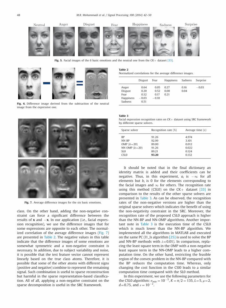
Fig. 5. Facial images of the 6 basic emotions and the neutral one from the CKþ dataset [33].

Fig. 6. Difference image derived from the subtraction of the neutralimage from the expressive one.

Fig. 7. Average difference images for the six basic emotions.

Table 2Normalized correlations for the average difference images.

Disgust Fear Happiness Sadness Surprise

Anger 0.64 0.05 0.27 0.16 �0.03Disgust 0.20 0.52 0.00 0.04Fear 0.52 0.17 0.21Happiness �0.03 �0.10Sadness 0.51

Table 3Facial expression recognition rates on CKþ dataset using SRC frameworkby different sparse solvers.

Sparse solver Recognition rate (%) Average time (s)

BP 91.26 4.974NN BP 92.99 3.101OMP (k¼20) 89.00 0.012NN OMP (k¼20) 91.26 0.022SL0 89.21 0.124CSL0 93.20 0.132

M.R. Mohammadi et al. / Signal Processing 100 (2014) 42–5048

class. On the other hand, adding the non-negative con-straint can force a significant difference between theresults of x and �x. In our application (i.e., facial expres-sion recognition), we use the difference images that forsome expressions are opposite to each other. The normal-ized correlation of the average difference images (Fig. 7)are presented in Table 2. The negative values in this tableindicate that the difference images of some emotions aresomewhat symmetric and a non-negative constraint isnecessary. In addition, due to subject variability and noise,it is possible that the test feature vector cannot representlinearly based on the true class atoms. Therefore, it ispossible that some of the other atoms with different signs(positive and negative) combine to represent the remainingsignal. Such combination is useful to sparse reconstructionbut harmful in the sparse representation-based classifica-tion. All of all, applying a non-negative constraint on thesparse decomposition is useful in the SRC framework.

It should be noted that in the final dictionary anidentity matrix is added and their coefficients can benegative. Thus, in this experiment, ai is �1 for allelements but bi is 0 for the elements corresponding tothe facial images and 1 for others. The recognition rateusing this method (CSL0) on the CKþ dataset [33] incomparison to the results of the other sparse solvers arepresented in Table 3. As can be observed, the recognitionrates of the non-negative versions are higher than theoriginal sparse solvers which indicates the benefit of usingthe non-negativity constraint in the SRC. Moreover, therecognition rate of the proposed CSL0 approach is higherthan the NN-BP and NN-OMP algorithms. Another impor-tant note in Table 3 is the execution time of the CSL0which is much lower than the NN-BP algorithm. Weimplemented all the algorithms in MATLAB and executedon the same PC (l1_ls algorithm [25] is used to solve the BPand NN-BP methods with λ¼0.01). In comparison, repla-cing the least square term in the OMP with a non-negativeleast square term in the NN-OMP leads to a higher com-putation time. On the other hand, restricting the feasibleregion of the convex problem in the NN-BP compared withthe BP reduces the computation time. Whereas, onlychanging the cost function in the CSl0 leads to a similarcomputation time compared with the SL0 method.

In this experiment, we use the following parameters forthe CSL0 algorithm: smin ¼ 10�5, K ¼ n=2¼ 135, L¼5, μ¼2,d¼0.75, and ε¼ 10�2.

M.R. Mohammadi et al. / Signal Processing 100 (2014) 42–50 49

5. Conclusion

In this paper a novel sparse solver with non-negativeconstraint was proposed that minimizes a weighted L0norm instead of L0 norm. In the weighted L0 norm, thepenalty of negative coefficients is larger than positive onesunlike L0 norm where the penalty of all non-zero coeffi-cients is equal. We proved that if the penalty of negativecoefficients is larger than a finite value, it is sufficient toforce all coefficients to be non-negative. The proposedalgorithm for optimizing the weighted L0 norm is based onConstraint Smoothed L0 norm (CSL0) that tries to mini-mize the discontinuous cost function in a coarse to fineapproach.

The proposed algorithm was evaluated on some simu-lated data that indicates the higher accuracy of theproposed algorithm in comparison with the state-of-the-art sparse solvers. Moreover, it is illustrated theoreticallythat the non-negative constraint for the application offacial expression recognition using SRC is useful. Theexperimental results support this theory and the facialexpression recognition rate using CSL0 is about 4% betterthan SL0.

Other constraints may be useful in other applications ofsparse representation. The formulation to apply otherconstraints is presented by generalization of the non-negative constraint.

Acknowledgments

The authors would like to express their sincere thanksto Prof. Jeffery Cohn for granting access to the CKþdatabase, and to Mr. Aboozar Ghaffari for his valuablecomments.

References

[1] M. Elad, M. Aharon, Image denoising via learned dictionaries andsparse representation, in: Proceedings of the 2006 IEEE ComputerSociety Conference on Computer Vision and Pattern Recognition,vol. 1, IEEE, 2006, New York, NY, USA, pp. 895–900. http://dx.doi.org/10.1109/CVPR.2006.142.

[2] T.V. Hoang, E.H.B. Smith, S. Tabbone, Edge noise removal in bilevelgraphical document images using sparse representation, in: Pro-ceedings of the 2011 18th IEEE International Conference on ImageProcessing (ICIP), IEEE, 2011, Brussels, Belgium, pp. 3549–3552.http://dx.doi.org/10.1109/ICIP.2011.6116482.

[3] M. Elad, J.-L. Starck, P. Querre, D.L. Donoho, Simultaneous cartoonand texture image inpainting using morphological componentanalysis (mca), Appl. Comput. Harmon. Anal. 19 (3) (2005)340–358, http://dx.doi.org/10.1016/j.acha.2005.03.005.

[4] M.-J. Fadili, J.-L. Starck, F. Murtagh, Inpainting and zooming usingsparse representations, Comput. J. 52 (1) (2009) 64–79, http://dx.doi.org/10.1093/comjnl/bxm055.

[5] O.G. Sezer, O. Harmanci, O.G. Guleryuz, Sparse orthonormal transforms for image compression, in:Proceedings of the 15th IEEEInternational Conference on Image Processing, 2008. ICIP 2008,IEEE, 2008, San Diego, California, USA, pp. 149–152. http://dx.doi.org/10.1109/ICIP.2008.4711713.

[6] M. Turkan, C. Guillemot, Sparse approximation with adaptive dictionary for image prediction, in: Proceedings of the 2009 16th IEEEInternational Conference on Image Processing (ICIP), IEEE, 2009,Cairo, Egypt, pp. 25–28. http://dx.doi.org/10.1109/ICIP.2009.5413923.

[7] D.L. Donoho, Compressed sensing, IEEE Trans. Inf. Theory 52 (4)(2006) 1289–1306, http://dx.doi.org/10.1109/TIT.2006.871582.

[8] P. Bofill, M. Zibulevsky, Underdetermined blind source separationusing sparse representations, Signal Process. 81 (11) (2001) 2353–2362,http://dx.doi.org/10.1016/S0165-1684(01)00120-7.

[9] Y. Li, S.-I. Amari, A. Cichocki, D.W. Ho, S. Xie, Underdetermined blindsource separation based on sparse representation, IEEE Trans. SignalProcess. 54 (2) (2006) 423–437, http://dx.doi.org/10.1109/TSP.2005.861743.

[10] R. Gribonval, S. Lesage, et al., A survey of sparse component analysisfor blind source separation: principles, perspectives, and newchallenges, in: 14th European Symposium on Artificial Neural Net-works, ESANN'06 Proceedings, 2006, pp. 323–330.

[11] J. Wright, A.Y. Yang, A. Ganesh, S.S. Sastry, Y. Ma, Robust facerecognition via sparse representation, IEEE Trans. Pattern Anal.Mach. Intell. 31 (2) (2009) 210–227, http://dx.doi.org/10.1109/TPAMI.2008.79.

[12] S.S. Chen, D.L. Donoho, M.A. Saunders, Atomic decomposition bybasis pursuit, SIAM J. Sci. Comput. 20 (1) (1998) 33–61, http://dx.doi.org/10.1137/S1064827596304010.

[13] S.G. Mallat, Z. Zhang, Matching pursuits with time–frequencydictionaries, IEEE Trans. Signal Process. 41 (12) (1993) 3397–3415,http://dx.doi.org/10.1109/78.258082.

[14] H. Mohimani, M. Babaie-Zadeh, C. Jutten, A fast approach for over-complete sparse decomposition based on smoothed ℓ0 norm, IEEETrans. Signal Process. 57 (1) (2009) 289–301, http://dx.doi.org/10.1109/TSP.2008.2007606.

[15] Y.C. Pati, R. Rezaiifar, P. Krishnaprasad, Orthogonal matching pursuit:recursive function approximation with applications to waveletdecomposition, in: Proceedings of the 1993 Conference Record ofthe Twenty-Seventh Asilomar Conference on Signals, Systems andComputers, IEEE, 1993, Pacific Grove, CA, pp. 40–44. http://dx.doi.org/10.1109/ACSSC.1993.342465.

[16] A. Eftekhari, M. Babaie-Zadeh, C. Jutten, H.A. Moghaddam, Robust-sl0 for stable sparse representation in noisy settings, in: Proceedingsof the IEEE International Conference on Acoustics, Speech andSignal Proces sing, 2009, ICASSP 2009, IEEE, 2009, Taipei, Taiwan,pp. 3433–3436. http://dx.doi.org/10.1109/ICASSP.2009.4960363.

[17] B. Wohlberg, Noise sensitivity of sparse signal representations:reconstruction error bounds for the inverse problem, IEEE Trans.Signal Process. 51 (12) (2003) 3053–3060, http://dx.doi.org/10.1109/TSP.2003.819006.

[18] E. Amaldi, V. Kann, On the approximability of minimizing nonzerovariables or unsatisfied relations in linear systems, Theor. Comput.Sci. 209 (1) (1998) 237–260, http://dx.doi.org/10.1016/S0304-3975(97)00115-1.

[19] R. Gribonval, M. Nielsen, Sparse representations in unions of bases,IEEE Trans. Inf. Theory 49 (12) (2003) 3320–3325, http://dx.doi.org/10.1109/TIT.2003.820031.

[20] P. Babu, K. Pelckmans, P. Stoica, J. Li, Linear systems, sparse solutions,and Sudoku, IEEE Signal Process. Lett. 17 (1) (2010) 40–42, http://dx.doi.org/10.1109/LSP.2009.2032489.

[21] D.L. Donoho, J. Tanner, Sparse nonnegative solution of underdeter-mined linear equations by linear programming, Proc. Natl. Acad. Sci.USA 102 (27) (2005) 9446–9451, http://dx.doi.org/10.1073/pnas.0502269102.

[22] J.A. Tropp, Greed is good: algorithmic results for sparse approxima-tion, IEEE Trans. Inf. Theory 50 (10) (2004) 2231–2242, http://dx.doi.org/10.1109/TIT.2004.834793.

[23] A.M. Bruckstein, M. Elad, M. Zibulevsky, On the uniqueness ofnonnegative sparse solutions to underdetermined systems of equa-tions, IEEE Trans. Inf. Theory 54 (11) (2008) 4813–4820, http://dx.doi.org/10.1109/TIT.2008.929920.

[24] R. Peharz, F. Pernkopf, Sparse nonnegative matrix factorization withℓ0-constraints, Neurocomputing 80 (2012) 38–46, http://dx.doi.org/10.1016/j.neucom.2011.09.024.

[25] S.-J. Kim, K. Koh, M. Lustig, S. Boyd, D. Gorinevsky, An interior-pointmethod for large-scale ℓ1-regularized least squares, IEEE J. Sel. Top.Signal Process. 1 (4) (2007) 606–617, http://dx.doi.org/10.1109/JSTSP.2007.910971.

[26] P.R. Gill, A. Wang, A. Molnar, The in-crowd algorithm for fast basispursuit denoising, IEEE Trans. Signal Process. 59 (10) (2011)4595–4605, http://dx.doi.org/10.1109/TSP.2011.2161292.

[27] J. Nocedal, S.J. Wright, Penalty and augmented lagrangian methods,in: Numerical Optimization, Springer Series in Operations Researchand Financial Engineering, Springer, New York, 2006, pp. 497–528.doi: http://dx.doi.org/10.1007/978-0-387-40065-5_17.

[28] I.F. Gorodnitsky, B.D. Rao, Sparse signal reconstruction from limiteddata using focuss: a re-weighted minimum norm algorithm, IEEETrans. Signal Process. 45 (3) (1997) 600–616, http://dx.doi.org/10.1109/78.558475.

M.R. Mohammadi et al. / Signal Processing 100 (2014) 42–5050

[29] D.L. Donoho, M. Elad, Optimally sparse representation in general(nonorthogonal) dictionaries via l1 minimization, Proc. Natl. Acad.Sci. 100 (5) (2003) 2197–2202, http://dx.doi.org/10.1073/pnas.0437847100.

[30] J. Wright, Y. Ma, J. Mairal, G. Sapiro, T.S. Huang, S. Yan, Sparserepresentation for computer vision and pattern recognition, Proc.IEEE 98 (6) (2010) 1031–1044, http://dx.doi.org/10.1109/JPROC.2010.2044470.

[31] H. Cheng, Z. Liu, L. Yang, X. Chen, Sparse representation and learningin visual recognition: theory and applications, Signal Process. 93 (6)(2013) 1408–1425, http://dx.doi.org/10.1016/j.sigpro.2012.09.011.

[32] P. Ekman, W.V. Friesen, Constants across cultures in the face andemotion, J. Personal. Soc. Psychol. 17 (2) (1971) 124.

[33] P. Lucey, J.F. Cohn, T. Kanade, J. Saragih, Z. Ambadar, I. Matthews, Theextended Cohn–Kanade dataset (ck+): a complete dataset for actionunit and emotion-specified expression, in: Proceedings of the 2010IEEE Computer Society Conference on Computer Vision and PatternRecognition Workshops (CVPRW), IEEE, 2010, San Francisco, CA,pp. 94–101. http://dx.doi.org/10.1109/CVPRW.2010.5543262.