Embed Size (px)
Citation preview

UNIVERSITY OF EAST ANGLIA
Non-Metric Multi-Dimensional
Scaling for Distance-Based
Privacy-Preserving Data Mining
by
Khaled S. Alotaibi
A thesis submitted to the School of Computing Sciences
of the University of East Anglia in partial fulfillment
of the requirements for the degree of
Doctor of Philosophy
January 2015
c©This copy of the thesis has been supplied on condition that anyone who consults
it is understood to recognise that its copyright rests with the author and that
no quotation from the thesis, nor any information derived therefrom, may be
published without the author’s prior written consent.

UNIVERSITY OF EAST ANGLIA
AbstractFaculty of Science
School of Computing Sciences
Doctor of Philosophy
by Khaled S. Alotaibi
Recent advances in the field of data mining have led to major concerns about
privacy. Sharing data with external parties for analysis puts private information
at risk. The original data are often perturbed before external release to protect
private information. However, data perturbation can decrease the utility of the
output. A good perturbation technique requires balance between privacy and
utility. This study proposes a new method for data perturbation in the context of
distance-based data mining.
We propose the use of non-metric multi-dimensional scaling (MDS) as a suit-
able technique to perturb data that are intended for distance-based data mining.
The basic premise of this approach is to transform the original data into a lower
dimensional space and generate new data that protect private details while main-
taining good utility for distance-based data mining analysis. We investigate the
extent the perturbed data are able to preserve useful statistics for distance-based
analysis and to provide protection against malicious attacks. We demonstrate that
our method provides an adequate alternative to data randomisation approaches
and other dimensionality reduction approaches. Testing is conducted on a wide
range of benchmarked datasets and against some existing perturbation methods.
The results confirm that our method has very good overall performance, is com-
petitive with other techniques, and produces clustering and classification results
at least as good, and in some cases better, than the results obtained from the
original data.

Acknowledgements
In the name of Allah, the most gracious, the most merciful.
Many thanks go to almighty Allah, who gave me the strength and ability to
complete this work.
I would like to express my gratitude to my supervisor Dr Beatriz De La Iglesia.
Dear Beatriz, thanks for your hospitality, help and guidance. I am much more
confident in accepting the challenge and leading my research due to the training
and the encouragement you provided during my study. Thanks for listening to
me whenever I was in trouble and thanks for your patience when discussing issues
and answering questions. I can never forget your support and help you provided
me whenever I need you. Without your ongoing professional support, this thesis
would not have been possible.
I would like also to take this opportunity to thank my secondary supervisors
Prof Vic Rayward-Smith and Dr Wenjia Wang for their insightful comments, sup-
port and advice. I was really lucky to be under their supervision. Both were
always there to help me with full enthusiasm and up to date knowledge.
A further special note of thanks must goes also to all colleagues in the School of
Computing Science at UEA and all friends from my homeland whom I meet here
in Norwich for their support and company. Special thanks to Dr Bander Almutairi
for his help in explaining some mathematical materials.
Many sincere thanks to my parents, brothers and sisters for sharing me personal
feelings, the best and the worst moments of my life. Finally, the most special
thanks goes to my beloved wife, Modhi, and children, Elaph, Jude, Farah and
Mohammed, for their love, support, and patience throughout all my academic
studies.
Khaled S. Alotaibi
January 2015
ii

Contents
Abstract i
Acknowledgements ii
List of Figures vi
List of Tables x
List of Publications xii
Abbreviations xiii
Symbols xv
1 Introduction 1
1.1 Motivation . . . . . . . . . . . . . . . . . . . . . . . . . . . . . . . . 3
1.2 Problem Description . . . . . . . . . . . . . . . . . . . . . . . . . . 5
1.3 Thesis Objectives . . . . . . . . . . . . . . . . . . . . . . . . . . . . 7
1.4 Thesis Contributions . . . . . . . . . . . . . . . . . . . . . . . . . . 7
1.5 Thesis Organisation . . . . . . . . . . . . . . . . . . . . . . . . . . . 8
2 Privacy-Preserving in Distance-Based Data Mining 10
2.1 Introduction . . . . . . . . . . . . . . . . . . . . . . . . . . . . . . . 11
2.2 Data Utility versus Privacy . . . . . . . . . . . . . . . . . . . . . . 13
2.3 Distance-based Data Mining . . . . . . . . . . . . . . . . . . . . . . 14
2.3.1 Distance Measures . . . . . . . . . . . . . . . . . . . . . . . 15
2.3.2 Properties of a Distance Metric . . . . . . . . . . . . . . . . 18
2.3.3 Distance Metrics for Numerical, Categorical andMixed Data . . . . . . . . . . . . . . . . . . . . . . . . . . . 19
2.3.3.1 Dissimilarities Between Numerical Data . . . . . . 20
2.3.3.2 Similarities of Categorical Data . . . . . . . . . . . 24
2.3.3.3 Similarities of Mixed Data . . . . . . . . . . . . . . 26
2.3.4 Distance-Based Tasks . . . . . . . . . . . . . . . . . . . . . . 28
iii

Contents iv
2.3.5 Neighbourhood Space of an Object . . . . . . . . . . . . . . 30
2.3.6 Decision Boundaries for Distance Metrics . . . . . . . . . . . 31
2.3.7 Transformation-Invariant Data Mining . . . . . . . . . . . . 33
2.4 Data Anonymisation Methods . . . . . . . . . . . . . . . . . . . . . 34
2.5 Data Randomisation Methods . . . . . . . . . . . . . . . . . . . . . 35
2.6 Dimensionality Reduction for Privacy-Preserving Data Mining . . . 37
2.6.1 Random Projection Perturbation . . . . . . . . . . . . . . . 37
2.6.2 PCA-based Perturbation . . . . . . . . . . . . . . . . . . . . 38
2.6.3 SVD-based Perturbation . . . . . . . . . . . . . . . . . . . . 39
2.6.4 Fourier Transform Perturbation . . . . . . . . . . . . . . . . 40
2.6.5 Attacks to Dimensionality Reduction . . . . . . . . . . . . . 41
2.7 ε-Distortion Mapping . . . . . . . . . . . . . . . . . . . . . . . . . . 43
2.8 The Need for Non-metric MDS Perturbation . . . . . . . . . . . . . 44
2.9 Summary . . . . . . . . . . . . . . . . . . . . . . . . . . . . . . . . 45
3 Non-Metric Multi-Dimensional Scaling Data Perturbation 47
3.1 Introduction . . . . . . . . . . . . . . . . . . . . . . . . . . . . . . . 48
3.2 MDS Preliminaries . . . . . . . . . . . . . . . . . . . . . . . . . . . 49
3.3 Non-Metric MDS Data Perturbation . . . . . . . . . . . . . . . . . 53
3.3.1 Monotonicity Preservation . . . . . . . . . . . . . . . . . . . 60
3.3.2 Distance Preservation . . . . . . . . . . . . . . . . . . . . . . 62
3.3.3 How Many Dimensions to Retain? . . . . . . . . . . . . . . . 64
3.3.4 Non-Metric MDS Algorithm . . . . . . . . . . . . . . . . . . 67
3.3.5 Numerical Example . . . . . . . . . . . . . . . . . . . . . . . 68
3.4 Geometry of Non-Metric MDS . . . . . . . . . . . . . . . . . . . . . 73
3.5 On the Proximity for Non-Metric MDS . . . . . . . . . . . . . . . . 75
3.6 Summary . . . . . . . . . . . . . . . . . . . . . . . . . . . . . . . . 76
4 Evaluation of Privacy and Information Loss 78
4.1 Introduction . . . . . . . . . . . . . . . . . . . . . . . . . . . . . . . 79
4.2 Information Loss Measure . . . . . . . . . . . . . . . . . . . . . . . 81
4.3 Uncertainty of Non-Metric MDS Solution . . . . . . . . . . . . . . . 85
4.4 Distance-Based Attack . . . . . . . . . . . . . . . . . . . . . . . . . 90
4.4.1 Metric Dimension Subspace . . . . . . . . . . . . . . . . . . 91
4.4.2 Distance-Based Attack Algorithm . . . . . . . . . . . . . . . 94
4.4.2.1 Non-linear Least-squares Method . . . . . . . . . . 94
4.4.2.2 Point Location Estimation using a Set of Distances 96
4.4.2.3 Numerical Example . . . . . . . . . . . . . . . . . 98
4.4.3 Disclosure Risk Measure . . . . . . . . . . . . . . . . . . . . 98
4.4.4 Experiments . . . . . . . . . . . . . . . . . . . . . . . . . . . 101
4.5 PCA-Based Attack . . . . . . . . . . . . . . . . . . . . . . . . . . . 108
4.5.1 Basics of PCA . . . . . . . . . . . . . . . . . . . . . . . . . . 108
4.5.2 PCA-Based Attack Algorithm . . . . . . . . . . . . . . . . . 110
4.5.3 Distortion Quantification of Eigenstructure . . . . . . . . . . 113

Contents v
4.5.4 Experiments . . . . . . . . . . . . . . . . . . . . . . . . . . . 114
4.6 Summary . . . . . . . . . . . . . . . . . . . . . . . . . . . . . . . . 123
5 Evaluation of Distance-Based Clustering and Classification 125
5.1 Introduction . . . . . . . . . . . . . . . . . . . . . . . . . . . . . . . 126
5.2 Application to Clustering Tasks . . . . . . . . . . . . . . . . . . . . 127
5.2.1 The Task of Distance-Based Clustering . . . . . . . . . . . . 127
5.2.2 Cluster Validity Evaluation . . . . . . . . . . . . . . . . . . 129
5.2.3 Experiments and Results . . . . . . . . . . . . . . . . . . . . 131
5.2.3.1 Datasets and Experimental Setup . . . . . . . . . . 131
5.2.3.2 Comparison of Clusterings . . . . . . . . . . . . . . 133
5.2.3.3 Statistical Significance Testing . . . . . . . . . . . 138
5.2.3.4 Utility versus Privacy . . . . . . . . . . . . . . . . 141
5.3 Application to Classification Tasks . . . . . . . . . . . . . . . . . . 146
5.3.1 k-Nearest Neighbours (k-NN) . . . . . . . . . . . . . . . . . 146
5.3.2 Support Vector Machine (SVM) . . . . . . . . . . . . . . . . 147
5.3.3 Utility Measures for Classification . . . . . . . . . . . . . . . 150
5.3.3.1 Neighbourhood Preservation . . . . . . . . . . . . . 151
5.3.3.2 Class Compactness . . . . . . . . . . . . . . . . . . 152
5.3.4 Experimental Results . . . . . . . . . . . . . . . . . . . . . . 153
5.3.4.1 Experimental Setup . . . . . . . . . . . . . . . . . 153
5.3.4.2 Comparing Accuracy of Classifiers . . . . . . . . . 155
5.3.4.3 Data Utility Measures . . . . . . . . . . . . . . . . 159
5.3.4.4 Privacy and Utility Assessment . . . . . . . . . . . 166
5.3.4.5 Statistical Testing . . . . . . . . . . . . . . . . . . 167
5.4 Summary . . . . . . . . . . . . . . . . . . . . . . . . . . . . . . . . 172
6 Conclusions and Future Work 174
6.1 Conclusions . . . . . . . . . . . . . . . . . . . . . . . . . . . . . . . 174
6.2 Limitations and Future Work . . . . . . . . . . . . . . . . . . . . . 177
A Triangle Geometry for Non-Metric MDS 181
Bibliography 188

List of Figures
1.1 Data outsourcing and sharing scenarios. . . . . . . . . . . . . . . . 6
2.1 A taxonomy of the main techniques used for PPDM. . . . . . . . . 12
2.2 Contour plot of the neighbourhood for a point at the origin (0, 0)using different distance measures. Contour lines close to (0, 0) havelow values, whereas further away lines have higher values. . . . . . . 22
2.3 Mahalanobis distances between the points represented by squaresand the remaining points represented by circles. The colour barrepresents how far the points represented by squares are from thepoints represented by circles. The more blue is the colour the closeris the point. . . . . . . . . . . . . . . . . . . . . . . . . . . . . . . . 23
2.4 An example of the decision boundary between two classes (blue andred) for linear data (a) and non-linear data (b). The hyperplane His the optimal decision boundary that separates the two classes.The region R1 denotes that part of input space classified as blue,while the region R2 is classified as red. . . . . . . . . . . . . . . . . 32
3.1 2-dimensional representation obtained from MDS analysis on a setof distances between some cities in the UK. . . . . . . . . . . . . . . 50
3.2 An example shows the effect of the non-metric MDS perturbationon the geometry of “Nefertiti” face at different dimensions. Thetop left is the original face. The following faces are the perturbedfaces at n − 5, n − 10, n − 20, n − 30, n − 40, n − 50 and n − 60dimensions, respectively. . . . . . . . . . . . . . . . . . . . . . . . . 56
3.3 Correlations among pairs of variables in: (a) the original data, X,and (b) the perturbed data, Y . Histograms of the variables appearalong the matrix diagonal; scatter plots of variable pairs appearoff-diagonal. . . . . . . . . . . . . . . . . . . . . . . . . . . . . . . . 58
3.4 Distribution of dissimilarities at the original data (top left), at 3-dimensions (top right), at 2-dimensions (bottom left) and at 1-dimension (bottom right). . . . . . . . . . . . . . . . . . . . . . . . 59
3.5 Three different datasets with different geometrical shapes. The toprow are the original data at 3-dimensional space. The bottom roware the perturbed data at 2-dimensional space using non-metric MDS. 65
vi
List of Figures vii
3.6 (a) The initial configuration in 3-dimensional space. (b) Shepardplot shows how the distances approximate the disparities (the scat-ter of blue circles around the red line), and how the disparities reflectthe rank order of the dissimilarities (the red line is non-linear butincreasing). . . . . . . . . . . . . . . . . . . . . . . . . . . . . . . . 69
3.7 The stress, S, at different iterations. . . . . . . . . . . . . . . . . . 72
3.8 (a) The final configuration in 3-dimensional space. (b) Shepard plotshows a perfect fit where the disparities are exactly coincided withthe distances. . . . . . . . . . . . . . . . . . . . . . . . . . . . . . . 72
3.9 Points arrangement for which the inequalities order is not violated. 74
4.1 (a) A representation of data in the original space, X. (b)-(d) Arepresentation of data in the (n − 1), (n − 2) and (n − 3) lowerdimensional spaces, Y1, Y2 and Y3, respectively. The red lines rep-resent the distortion in distances, as result of the non-metric MDStransformation, which is quantified by the stress. . . . . . . . . . . . 83
4.2 Shepard plot of dissimilarities, δij, against distances, dij, for solu-tions obtained by non-metric MDS at different dimensions, n. . . . 84
4.3 Representation of all possible positions (shaded area) to place thepoint b, without violating the constraint specified for each case. . . 86
4.4 A representation of placing point x on (a) a line and (b) a circlewithout violating the ordering constraint. . . . . . . . . . . . . . . . 87
4.5 A representation of uncertainty about placing point x in n-dimensionalspace. . . . . . . . . . . . . . . . . . . . . . . . . . . . . . . . . . . 88
4.6 Trilateration example in 2-dimensional space. . . . . . . . . . . . . 93
4.7 95% confidence ellipse to show the effect of outliers on point locationestimation. The outliers are distinguished by red circles. The opencircle is the data mean. . . . . . . . . . . . . . . . . . . . . . . . . . 97
4.8 (a) An estimated location for point x starting from point (0, 0). (b)A function of the relative error at each iteration, k. . . . . . . . . . 99
4.9 (a) An estimated location for point x starting from random point.(b) A function of the relative error at each iteration, k. . . . . . . . 99
4.10 Data points in the original space, X, and the perturbed space, Y .The dashed line are the Euclidean distances. . . . . . . . . . . . . . 101
4.11 (a) Average error (red line) of distance-based attack in locatingunknown point x in the perturbed data, Y along with the lowerand upper bounds (blue lines). (b) Average error of estimating thelocation of an unknown point, x, at different dimensions in Y . . . . 102
4.12 Average privacy (ρ) against distance-based attack versus stress (S)at different dimensions using different perturbation techniques. Thebold line is stress and the dashed line is average privacy. . . . . . . 106
4.13 Average privacy (ρ) against distance-based attack at different di-mensions using different numbers of the known points. . . . . . . . 107
4.14 Estimated location error at different iterations, k, using differentsizes of noisy measures for the n+ 1 known points. . . . . . . . . . 107

List of Figures viii
4.15 Estimated error at different dimensions, p, using zero-valued fea-tures up-scaling, random-valued features up-scaling and distance-preserving features up-scaling. . . . . . . . . . . . . . . . . . . . . . 107
4.16 (a) Plot of data values of the original data and the perturbed data.(b) The effectiveness of PCA-based attack in recovering the originaldata. . . . . . . . . . . . . . . . . . . . . . . . . . . . . . . . . . . . 115
4.17 (a) Average distance error between the original and recovered dataat different dimensions. (b) The average distance error when usingdifferent sizes of the known sample. . . . . . . . . . . . . . . . . . . 116
4.18 Average distance error between the original data, X, and the recov-ered data, X ′ at different dimensions using different perturbationmethods. . . . . . . . . . . . . . . . . . . . . . . . . . . . . . . . . . 118
4.19 Stress at different dimensions using different perturbation methods. 119
4.20 Sample covariance matrix with 95% tolerance ellipses for the orig-inal data, X. The 10%,20% and 30% ellipses represent the changein the covariance matrix when 10%,20% and 30% samples, respec-tively, from the original data are replaced by their perturbed sam-ples from the perturbed data using different transforms (a)-(f). . . . 122
5.1 The variation of information (V I) of RP, PCA, SVD, NMDS andDCT using k-means. . . . . . . . . . . . . . . . . . . . . . . . . . . 135
5.2 The variation of information (V I) of RP, PCA, SVD, NMDS andDCT using hierarchical clustering. . . . . . . . . . . . . . . . . . . . 136
5.3 The variation of information (V I) of RP, PCA, SVD, NMDS andDCT using DBSCAN. . . . . . . . . . . . . . . . . . . . . . . . . . 137
5.4 Average privacy (ρ) achieved against distance-based attack for vary-ing p using different perturbation methods. . . . . . . . . . . . . . . 142
5.5 Average privacy achieved against PCA-based attack for varying pusing different perturbation methods. . . . . . . . . . . . . . . . . . 145
5.6 Linear SVM classifier. The decision boundary is the solid line, whiledotted lines bound the maximal margin of width 2/||w||. For non-separable case (b), the points labelled ξi on the wrong side of theirmargin 1/||w|| are the slack variables which count ξ/||w||. Themargin is maximised subject to Σ ξi ≤ constant. . . . . . . . . . . . 148
5.7 The impact of the transformation on classifying example x wherethe distances of 3-nearest neighbours have been changed. In theoriginal data (a), the example is classified as “negative” whereas inthe perturbed data (b) it is classified as “positive”. . . . . . . . . . 151
5.8 A classification accuracy of k-NN on the original data, X, and theperturbed data, Y , produced by RP, PCA, SVD, NMDS and DCTat different dimensions, p. . . . . . . . . . . . . . . . . . . . . . . . 156
5.9 Classification accuracy of linear SVM at different dimensions, p,using the original data, X, and the perturbed data, Y , producedby RP, PCA, SVD, NMDS and DCT. . . . . . . . . . . . . . . . . . 157
5.10 Average classification accuracy of non-linear SVM using three dif-ferent kernels: Polynomial, RBF and Multilayer Perceptron. . . . . 158
List of Figures ix
5.11 (a) Neighbourhood preservation and (b) class compactness at dif-ferent dimensions in the perturbed data, Y , using different pertur-bation techniques. . . . . . . . . . . . . . . . . . . . . . . . . . . . . 160
5.12 A comparison of class compactness between data objects in (a) theoriginal data, X, and the perturbed data, Y , generated by differ-ent methods (b) - (f). The classes in PCA and NMDS solutionsare reasonably well separated relative to the classes in the othersperturbation methods. . . . . . . . . . . . . . . . . . . . . . . . . . 164
5.13 Critical difference diagram of the average ranks for k-NN classifierover the perturbed data using five perturbation techniques (CD =1.58). . . . . . . . . . . . . . . . . . . . . . . . . . . . . . . . . . . . 168
5.14 Critical difference diagram of the average ranks for linear SVM overthe perturbed data, derived from the results in Table 5.12 (CD =1.53). . . . . . . . . . . . . . . . . . . . . . . . . . . . . . . . . . . . 170
5.15 Critical difference diagram of the average ranks for k-NN classifierat one reduced dimension, n− 1, (CD = 1.98). . . . . . . . . . . . . 171
A.1 Representation of all possible positions (shaded area) to place thepoint b, without violating the constraint: (a) dab ≤ dbc ≤ dac and(b) dab ≤ dac ≤ dbc. . . . . . . . . . . . . . . . . . . . . . . . . . . . 182
A.2 Uncertainty boundary to place a point b under the constraint dab ≤dbc ≤ dac. . . . . . . . . . . . . . . . . . . . . . . . . . . . . . . . . 185
A.3 Uncertainty boundary to place a point b under the constraint dab ≤dac ≤ dbc. . . . . . . . . . . . . . . . . . . . . . . . . . . . . . . . . 186

List of Tables
2.1 An example of five data objects in 2-dimensional space. . . . . . . . 24
2.2 Mahalanobis distance between the data objects in data X and theobjects y1, y2 and y3. . . . . . . . . . . . . . . . . . . . . . . . . . . 24
3.1 Distances between 10 UK citites. . . . . . . . . . . . . . . . . . . . 49
3.2 Iris dataset: data values of the first 10 rows in 4-dimensional space(original data X) and 3-dimensional space (perturbed data Y ). . . 57
3.3 Basic statistics of Iris dataset before and after the perturbation. . . 57
3.4 Correlations between variables in (a) the original data, X, and (a)the perturbed data, Y . . . . . . . . . . . . . . . . . . . . . . . . . . 58
3.5 Derivation of disparities using PAV algorithm. . . . . . . . . . . . . 61
3.6 Kruskal’s rule to decide on the quality of the lower-dimensional space. 66
3.7 Stress values at one reduced dimension using Minkowski distancewith different exponents. . . . . . . . . . . . . . . . . . . . . . . . . 66
3.8 Predicted disparities, dij, using PAV algorithm. . . . . . . . . . . . 70
4.1 Original and perturbed data values. . . . . . . . . . . . . . . . . . . 100
4.2 Benchmark datasets used in our experiments. . . . . . . . . . . . . 103
4.3 Average change in eigenvalues’ scale using different sizes of theknown sample. The best result for each dataset is shown in bold. . 121
4.4 Average change in eigenvectors’ orientation using different sizes ofthe known sample. The best result for each dataset is shown in bold.121
5.1 A contingency table: Clustering C × C ′ . . . . . . . . . . . . . . . . 130
5.2 A description of datasets used in our experiments. . . . . . . . . . . 132
5.3 The observed p-value of paired t-test using k-means. The p-valuesless than 5% (bold faced) indicate that the results are statisticallydifferent at the 95% confidence level. . . . . . . . . . . . . . . . . . 139
5.4 A statistical comparison of the performance of NMDS and othermethods using paired t-test. The bold faced p-values indicate noadvantage gained from using NMDS compared to the other pertur-bation methods. . . . . . . . . . . . . . . . . . . . . . . . . . . . . . 140
5.5 Observed p-values of paired t-test of V I for NMDS against the othermethods using different number of clusters, k. . . . . . . . . . . . . 141
5.6 Neighbourhood preservation in the perturbed data, Y , using differ-ent number of k neighbours. . . . . . . . . . . . . . . . . . . . . . . 161
x

List of Tables xi
5.7 A comparison of class compactness in the original data, X, and theperturbed data, Y , at different number of k. . . . . . . . . . . . . . 161
5.8 Average neighbourhood preservation for data points in the per-turbed data, Y , when consider variations of k from 3 to 10 usingfive perturbation techniques (RP, PCA, SVD, NMDS and DCT).The best result for each dataset is shown in bold. . . . . . . . . . . 162
5.9 Average class compactness in the original data, X and the per-turbed data, Y , when consider variations of k from 3 to 10 usingdifferent transformations. The best result for each dataset is shownin bold. . . . . . . . . . . . . . . . . . . . . . . . . . . . . . . . . . 163
5.10 RMSE of computing the dot product in the perturbed data, Y , atdifferent dimensions, p, using different perturbation techniques. . . . 165
5.11 Average classification accuracy (%) and (rank) of k-NN using fiveperturbation techniques (RP, PCA, SVD, NMDS and DCT). . . . . 168
5.12 Average classification accuracy (%) and (rank) of linear SVM usingfive perturbation techniques (RP, PCA, SVD, NMDS and DCT). . . 169
5.13 Classification accuracy (%) and (rank) of k-NN at one reduced di-mension. . . . . . . . . . . . . . . . . . . . . . . . . . . . . . . . . . 171

List of Publications
• K. Alotaibi, V. Rayward-Smith, and B. de la Iglesia. Nonmetric multidimen-
sional scaling: A perturbation model for privacy-preserving data clustering.
Statistical Analysis and Data Mining, 7(3):175-193, 2014.
• K. Alotaibi and B. de la Iglesia. Privacy-preserving SVM classification us-
ing non-metric MDS. In The Seventh International Conference on Emerging
Security Information, Systems and Technologies, Barcelona, Spain, pages
30-35. IARIA XPS Press, 2013.
• K. Alotaibi, V. J. Rayward-Smith, W. Wang, and B. de la Iglesia. Non-
linear dimensionality reduction for privacy-preserving data classification. In
Proceedings of IEEE Fourth International Conference on Privacy, Security,
Risk and Trust (PASSAT 2012), Amsterdam, The Netherlands, pages 694-
701. IEEE, 2012.
• K. Alotaibi, V. Rayward-Smith, and B. de la Iglesia. Non-metric multidi-
mensional scaling for privacy-preserving data clustering. In Intelligent Data
Engineering and Automated Learning-IDEAL 2011, Norwich, UK, pages
287-298, Berlin, Heidelberg, 2011. Springer.
xii

Abbreviations
CC Class Compactness
CD Critical Difference
DCT Discrete Cosine Transform
EM Expectation Maximisation
FT Fourier Transform
ICA Independent Component Analysis
ISOMAP ISOmetric Mapping
K-NN K-nearest Neighbour
KDD Knowledge Discovery in Databases
LLE Local Linear Embedding
LMDS Local Multidimensional Scaling
MAP Maximum Posteriori Probability
MDS Multidimensional Scaling
MI Mutual Information
NP Neighbourhood Preservation
PAV Pooled-Adjacent-Violator
PC Principle Component
PCA Principle Component Analysis
PPDM Privacy-prserving Data Mining
QID Quasi-identifier
RMSE Root Mean Squared Error
RP Random Projection
SDB Statistical Database
SDC Statistical Disclosure Control
xiii

Abbreviations xiv
SMC Secure Multiparty Computation
SSE Sum of Squared Error
SVD Singular Value Decomposition
SVM Support Vector Machine
VI Variation of Information

Symbols
Symbol Description
i, j indices of data object
m number of data objects
n number of dimensions in the original space
p number of dimensions in the perturbed space
X original data matrix
Y perturbed data matrix
C a set of classes/partitions, interchangeably
R real numbers space
xi data object in the original space
yi data object in the perturbed space
dij the distance between object i and object j
dij the disparity between object i and object j
T transformation/table, interchangeably
S∗ raw stress
S a set of sensitive attributes/stress, interchangeably
eij mapping error from object i to object j
k number of nearest neighbours/clusters/first PC, interchangeably
t number of iterations
ci centroid/class label, interchangeably
R random/projection/noise matrix, interchangeably
I identity matrix
u eigenvector
fX(x) probability distribution of variable X
xv

Symbols xvi
F (x) cumulative distribution of variable X
pdf probability density function
cdf cumulative distribution function
P (E) probability of event E
E expected value
AT transpose of matrix A
A−1 inverse of matrix A
H hyperplane
H0 null hypothesis
H1 alternative hypothesis
O(n) complexity time of order n
X estimate of data X
X ′ recovered data
md matching distance
M number of dissimilarities δij
N number of samples/unknown points/transforms, interchangeably
G(Ci, Cj) proximity of cluster Ci and cluster Cj
H(X) entropy of variable X
MI(X, Y ) mutual information between variable X and Y
||xi − xj|| Euclidean distance (L2 norm)
V ol(x) volume of object x
dim(G) metric dimension of subspace G
corr(Xi, Xj) correlation between variable Xi and variable Xj
U eigenvectors matrix
Uk a set of the k-nearest neighbours
w weight vector
K(u,v) kernel function
〈u,v〉 inner product
rank(A) rank of A
N(v) null space of vector v
acc(X) accuracy of learning model on data X

Symbols xvii
∆ dissimilarity matrix
δij the dissimilarity between object i and object j
ΣA covariance matrix of data matrix A
λ eigenvalue
ε distortion
ρ∗ privacy measure for a single point
ρ overall privacy measure
∇g(x) gradient of function g
σ standard deviation
σ2 variance
µ mean
α downhill step-size/angle between vectors/significance level, interchangeably
ξ slack variable
Φ transformation into Hilbert space
φ(X) information loss of data X

To my parents, wife and childrenwith sincere love and respect...
xviii

Chapter 1
Introduction
Modern technology enables easy storage and processing of large amounts of data
relating to everyday activities, such as making a phone call, buying an item from
a shop, and visiting a doctor. Data mining aims to discover new knowledge about
an application domain, utilising huge amounts of data from within that domain.
Typically, these data represent various individual entities such as persons, compa-
nies, and transactions. Driven by mutual benefits or by regulations that require
certain data to be cooperatively analysed, there is a demand for the exchange and
analysis of data between diverse parties. Data in their original form, however,
typically contain sensitive information about individuals or other confidential in-
formation, and analysing or sharing such data would violate individual privacy
and risk disclosing the confidential information.
There is a growing anxiety about personal information being open to potential
misuse. This is not necessarily limited to sensitive data, such as medical and
genetic records. Other personal information, although not as sensitive as health
records, can also be considered to be confidential and vulnerable to malicious
exploitation. For example, the publication of Netflix data, which contained movie
ratings of a large number of subscribers led to substantial controversy regarding
the identification of individuals and their preferences [123]. Public concern is
mainly focused on the so-called secondary use of personal information without the
consent of the individual. Consumers feel strongly that their personal information
should not be made available to other organisations without their prior consent.
The term “Privacy-Preserving Data Mining” (PPDM) has no single definition
or meaning. One possible definition is a method that obtains valid data mining
results without revealing the underlying data values. Generally, PPDM aims to
achieve two fundamental objectives—data privacy and utility. That is, producing
1

Chapter 1. Introduction 2
accurate mining results without disclosing “private” information. These two ob-
jectives are contradictory in nature. Many completely different approaches have
been proposed to tackle privacy preservation in the context of retaining utility
and privacy. However, in most cases, the proposed methods make a trade-off be-
tween these two objectives instead of providing a perfect solution that meets them
altogether.
Data perturbation methods are concerned with distorting the original values
and producing new data that have similar properties to the original data as much
as possible while preserving privacy. The perturbation process can be performed
using a number of transformations or modifications. However, some modifications
can reduce the granularity of representation and downgrade the information em-
bedded in the data and resulting in low data utility. In distance-based data mining,
the algorithm usually optimises a criterion function, which is often described in
terms of the interpoint distances between data objects. That is, the choice of
which clusters/classes to assign to a data point is determined by a similarity or
distance function. Intuitively, in such cases, data mining results will be influenced
by the objects’ distances to other objects. If the distances are well preserved, the
data utility will be high for the data mining algorithm, and more accurate results
can be obtained.
Non-metric multi-dimensional scaling (MDS) is an exploratory technique used
to visualise proximities in lower dimensional space [21]. It allows insight into the
underlying structure of relationships between data objects by providing a geo-
metrical representation of these relationships in lower dimensionality. The input
for non-metric MDS is the relationship between a pair of data objects, which are
interpreted as either similarity or dissimilarity measures. These relationships are
non-linearly transformed into a set of data points in a lower dimensional space
where each point represents an object in the higher dimensional space. The re-
sulting data have altered data values from the original values, yet they preserve
many distance-related properties. We are interested in PPDM in particular, for
application to distance-based data mining. In this context, non-metric MDS may
provide privacy by perturbing the data into a lower dimensional space with dis-
guised data values while retaining the distance relationships between objects.
Our approach is largely inspired by recent work on data perturbation [26, 101,
110, 121, 174]. However, our method differs significantly from the method used to
transform original data and produce perturbed data, which can then be published
or shared for data mining. It considers data attributes confidential data and

Chapter 1. Introduction 3
attempts to generate perturbed data that retain distance information.
1.1 Motivation
Technology has enabled an exponential rise in an organisation’s ability to gather,
store, and share large quantities of data. As large scale applications of data mining
become more common, there are large amounts of data stored in many databases
worldwide. The IBM Multinational Consumer Privacy Survey [146] published in
1999 illustrates public awareness towards privacy in online transactions. The key
finding from among the more than 3,000 people who responded in the United
States, the United Kingdom, and Germany is a clear desire for merchants and
service providers to properly address privacy concerns and establish policies that
strengthen trust and confidence. Most respondents (80%) feel that consumers have
lost control over how personal information is collected and used by companies. The
majority of respondents (94%) are concerned about the possible misuse of their
personal information. This survey also demonstrates that, when it comes to the
confidence that their personal information is properly handled, consumers have
the most trust in health care providers and banks and the least trust in credit
card agencies and internet companies.
Data mining techniques are used for many purposes, such as medical research,
financial fraud, counter-terrorism, national security, etc. Many of those applica-
tions may be highly beneficial for society and individuals. Government and private
organisations may wish to exploit their data in this way, but privacy and confi-
dentiality considerations stand in the way of fully utilising the benefits of such
services and architectures [60]. In this context, the concept of PPDM has become
more significant.
Allowing access to data in original form without any protection may indeed
violate privacy constraints. For example, a theft of information regarding more
than 163,000 consumers was reported in 2005 at ChoicePoint [35], which maintains
and sells personal information for government and industry. The firm has been
charged $10 million for not providing sufficient protection for the data it holds.
Another privacy breach occurred at Acxiom [135], which offers marketing and
information management services to companies for competitive purposes. In 2003,
over 1.6 billion customer records were stolen during the transmission of information
to and from Acxiom’s clients. A further example is the publication of Netflix data,
which contained 100 million ratings for 18,000 movie titles from 480,000 randomly

Chapter 1. Introduction 4
chosen users. In 2006, Netflix announced a challenge with a $1 million prize for
the participants that could improve its recommendation system based on client
preferences [10]. In 2007, Narayanan and Shmatikov [123] were able to identify
individual users by matching the datasets with movie ratings.
In 2003, SIGKDD (an ACM special interest group on knowledge discovery and
data mining) issued a letter (“Data Mining” is NOT Against Civil Liberties) [130]
to eliminate some misguided impressions regarding privacy concerns in the applica-
tions of data mining. The letter stated that data mining is concerned with analysis
techniques and is separate from issues of data collection and data aggregation. It
also pointed out the following:
“However, the best (and perhaps only) way to overcome the “limita-
tions” of data mining techniques is to do more research in data mining,
including areas like data security and privacy-preserving data mining,
which are actually active and growing research areas.”
The issue of privacy has been investigated from different aspects. One direc-
tion of the work is data anonymisation, which concentrates on reducing the risk
of identifying individuals using key attributes (known as quasi-identifiers) or the
private information held in certain sensitive attributes. Many methods based on
data anonymisation were proposed in literature [13, 59, 158] to prevent such link-
age attacks. Although data anonymisation can provide good privacy protection,
the data mining results can compromise the privacy of the original data [139].
Moreover, some anonymisation methods may alter attribute distribution and also
affect the distance between data objects [3].
Another research direction utilises the techniques of data randomisation to dis-
guise sensitive data by randomly modifying the data values, often using additive
or multiplicative noise. In fact, the size of the noise added to an individual value
gives an indication of the difficulty in recovering the original values. Thus, using
sufficiently high levels of noise may provide good privacy protection. However,
the most significant inadequacy of some data randomisation methods is that dis-
tances between data objects are not always preserved, leading to reduced accuracy
for distance-based data mining tasks [25]. Another drawback is the possibility of
separating the noise from the perturbed data by studying the spectral properties
of the data to estimate the random matrix and then estimate the original data
values [25].

Chapter 1. Introduction 5
A further direction uses data transformation approaches, such as dimension-
ality reduction, which seeks a meaningful representation of the original data in
some lower dimensional space. We will discuss these approaches in more detail
in Chapter 2. Ideally, to guarantee the suitability of the transformed data for
PPDM, both utility and privacy should be quantified and measurable.
We believe that any PPDM model should be task-specific since generic solutions
would be ineffective at achieving the required utility for the data mining task.
For instance, k-means clustering relies heavily on the Euclidean distance between
objects while attribute distribution would be more interesting than distances when
building a decision tree.
This research aims to develop a new method for PPDM that can overcome the
inadequacies of the above approaches. The new perturbation method offers mul-
tiple advantages over the existing methods used for the same purpose. First, it
preserves information for distance-based data mining tasks leading to more accu-
rate results. Second, it produces the perturbed data under uncertain conditions,
limiting the disclosure risk as much as possible. Third, it does not require any
modification on the existing data mining algorithms, as all of the modifications
remain limited to the original data.
1.2 Problem Description
The main focus of our work is to ensure that outsourcing or sharing data for certain
types of computations does not compromise the privacy of the original data. It is a
very common practice for organisations with limited computational resources and
lack of in-house expertise to outsource their data and operations to third party
service providers, which can offer storage resources and large scale computations.
For example, a supermarket chain may release its operational transactional data
to a third party to learn useful patterns of customer buying behaviour. In this
example, the supermarket chain is the data owner and the third party is referred
to as a service provider.
Another important issue arises when the data owner has his or her own private
data and would like to make it publicly available for one or more external parties
to obtain benefits from the analysis personally or for the third party. For instance,
hospitals in California are required by law to accurately report patient information
to be used by the government and private sector for decision-making regarding
healthcare [126].

Chapter 1. Introduction 6
Service Provider
Data Owner
Original Data
X
Perturbed Data
Y
External Parties
Data Users
Y
Analysis Results
Perturbed Data
Y
Figure 1.1: Data outsourcing and sharing scenarios.
Such scenarios may lead to privacy breach. This demonstrates the value of
data and the need to protect it. In the context of PPDM, perturbation techniques
may provide some of the necessary protection. That is, the perturbed data can
be published, manipulated, and mined without compromising the privacy of the
original data. A typical graphical representation of data outsourcing and sharing is
illustrated in Figure 1.1. The data owner can be any public or private organisation
who holds the original data, performs the perturbation, and releases the perturbed
data to the service provider who will conduct data mining on the perturbed data.
The service provider can also allow users to access the perturbed data or the results
of analysis.
In the other scenario, the data owner may share the computation with external
parties so that s/he can enable them to access the perturbed data and perform the
required analysis yet learn nothing about the original data values. This scenario
is relatively similar to privacy-preserving distributed data mining [87, 167], in
which the data are assumed to be distributed horizontally or vertically over many
different sites and the data mining is performed at one predefined site. However,
the scenario we are interested in makes no particular assumptions, but describes
ordinary access to the data hosted by the data owner.

Chapter 1. Introduction 7
1.3 Thesis Objectives
This research will examine the issue of privacy preservation for distance-based
data mining and propose a new perturbation method to sanitise the original data.
Particularly, we hypothesise that non-metric MDS is a good tool for distance-based
PPDM. To assess this, the perturbed data will be examined in terms of data utility
and privacy, and the overall performance of our method will be compared with
existing methods. The main objectives are summarised as follows:
1. Propose a perturbation method using non-metric MDS to perturb the orig-
inal data and explore its characteristics for PPDM (Chapter 3).
2. Examine and evaluate the privacy and utility associated with the proposed
method and compare the results with existing perturbation techniques (Chap-
ter 4).
3. Examine and evaluate the usefulness of the perturbed data for distance-based
data mining tasks using a set of real-world datasets, and compare against
existing perturbation techniques (Chapter 5).
1.4 Thesis Contributions
In this study, we propose a task-specific PPDM perturbation method based on
non-metric MDS. We evaluate our method in the context of k-means clustering,
hierarchical clustering, density-based clustering, k-nearest neighbour classification
(k-NN), and Support Vector Machine (SVM) with different kernels. The overall
performance of our method is compared with some existing dimensionality reduc-
tion methods including random perturbation [110, 129], PCA-based approaches
[11, 174], SVD-based approaches [101, 178], and Fourier transforms [121]. The
main contributions of this study are summarised as follows:
1. We introduce non-metric MDS as perturbation tool for distance-based data
mining tasks (Chapter 3).
2. We investigate two potential adversary attacks: a distance-based attack (Sec-
tion 4.4) and a PCA-based attack (Section 4.5) and use specific measures to
quantify the associated privacy. We show how these attacks would fail to
disclose the original data values since our perturbation technique effectively

Chapter 1. Introduction 8
downgrades the information embedded in the perturbed data and limits dis-
closure risk.
3. We show that perturbation using non-metric MDS preserves utility for dis-
tance-based data mining tasks. We evaluate our method using a number
of clustering and classification algorithms and compare the overall perfor-
mance with other well-known perturbation methods (Sections 5.2 and 5.3).
We propose a number of metrics to measure the size of distance distortion
caused by the perturbation in the original and perturbed spaces and to as-
sess neighbourhood preservation and group compactness before and after the
perturbation. The results demonstrate reliable performance of our method
in comparison with the other methods.
4. For each privacy attack, we investigate to what extent our method is able
to provide a trade-off between privacy and utility at different number of
dimensions (Sections 4.4.4 and 4.5.4). Similarly, we investigate the trade-
off between the privacy and the accuracy of data mining model at different
number of dimensions (Sections 5.2.3.4 and 5.3.4.4). We demonstrate that
the desired trade-off between privacy and utility level can be determined
according to the data owner’s preference.
1.5 Thesis Organisation
This section outlines the remainder of the thesis and briefly introduces the main
topics addressed in each chapter.
Chapter 2 offers an overview of privacy preservation in the context of distance-
based data mining. It discusses some essential concepts of distance-based data
mining and reviews the properties of certain distance metrics. It also introduces
various privacy-preserving techniques and methods that have been developed in
literature and explores their limitations and drawbacks.
Chapter 3 presents a privacy-preserving method and describes the rationale
for non-metric MDS, its mechanism, and its geometric characteristics.
Chapter 4 addresses the issue of privacy and utility of the perturbed data.
It discusses the issue of information loss and suggests a measure to quantify the
distortion caused by the perturbation. It also describes the concept of the uncer-
tainty produced by non-metric MDS and investigates how the perturbed data are
resilient to some potential privacy attacks, developed especially for this purpose.

Chapter 1. Introduction 9
Different measures are proposed to measure the disclosure risk of the perturbed
data.
Chapter 5 evaluates the privacy-preserving method in the context of distance-
based data mining and explores its suitability using different clustering and classi-
fication algorithms. It tests and compares the overall performance of the proposed
method with other perturbation techniques through a set of experiments. This
chapter also discusses the trade-off between privacy and utility in terms of the
accuracy of data mining models.
Chapter 6 summarises the thesis, discusses the research limitations, and out-
lines directions for future work.

Chapter 2
Privacy-Preserving in
Distance-Based Data Mining
The privacy issue in data mining began to be addressed after 2000 [7]. Over
the past several years, a large and growing number of methods were proposed
in this area both of theoretical and applied nature, several of which aim to ob-
tain valid data mining results while preserving privacy as much as possible. This
chapter describes the concept of distance-based data mining as well as some re-
lated topics, including distance metrics, mining tasks, neighbourhood preservation
and invariance of transformation. It also reviews the existing techniques used for
privacy-preserving data mining and outlines their related research issues.
This Chapter is organised as follows. Section 2.1 introduces some definitions
and general objectives of privacy-preserving data mining. Section 2.2 describes the
concept of data utility and its impact on the effectiveness of the privacy model.
Section 2.3 reviews distance-based data mining and defines some related concepts
and properties. Section 2.4 considers the methods and the techniques used in
data anonymisation, and discusses their potential attacks. The methods used for
data randomisation and the different attacks to those methods are presented in
Section 2.5. Section 2.6 introduces dimensionality reductions methods used for
PPDM and discuses some potential privacy attacks to these methods. Section
2.7 briefly describes the concept of space distortion. Section 2.8 presents the main
characteristics of our method. Finally, a summary of the chapter is given in Section
2.9.
10

Chapter 2. Privacy-Preserving in Distance-Based Data Mining 11
2.1 Introduction
Privacy is becoming an increasingly important issue, especially with respect to
counter-terrorism and national security; these may require the creation of personal
profiles and the construction of social network models in order to detect terrorist
communications in a distributed privacy-sensitive multi-party data environment.
Recent advances in the data mining field have also led to increased concerns about
privacy. Clifton et al. [33] argue that data mining techniques are considered a
challenge to privacy preservation since their accurate results depend on the use
of sensitive information about individuals. Therefore, there is a crucial need to
build algorithms that can mine data while guaranteeing that the privacy of the
individuals is not compromised. As defined in Chapter 1, PPDM attempts to
obtain valid data mining results without disclosing the underlying data values.
Data privacy in data mining refers to the keeping of all private or confidential
data secret. Although the concept of what is meant by privacy is not clearly de-
fined, Vaidya and Clifton [168] provided a roadmap for defining and understanding
privacy constraints. In their work, the term “privacy” is discussed in relation to
three different aspects: keeping information about individuals from being available
to others, protecting information from being misused, and protecting information
about a collection of data rather than just an individual (corporate privacy). In
accordance with these, many completely different approaches to privacy preserving
data mining have been proposed. However, all of them share the same generic goal,
which is to produce accurate mining results without disclosing private information.
The privacy threats caused by data mining can be viewed from two perspectives
[33]. The first is when the original data are published to external parties; if the
publication is conducted without any restrictions, privacy could be compromised.
For instance, publishing some medical data of patients in a hospital could lead
to identifying the patients. The second is once the data are analysed using the
data mining techniques, the output results themselves may violate privacy. For
example, the association rules or classification rules can compromise the privacy
of the data.
The ultimate goal of PPDM is to strive for a win-win-win situation: extracting
useful knowledge from the data, protecting the individual’s privacy, and preventing
any misuse or disclosure of the data. The research community in this field has
begun to address all these issues from two points of view—data perturbation and
the separation of authority. Data perturbation aims to provide modified data

Chapter 2. Privacy-Preserving in Distance-Based Data Mining 12
Perturbation-Based Approaches
Data Anonymization
Data Randomization
Cryptography-Based Approaches
Vertically Partitioned
Data
Horizontally Partitioned
DataDimensionality
Reduction
Secure Communication Protocols Multiplicative
Hybrid
Additive
SVD
PCA
Fourier Transform
Non-metric MDS
l-diversity
t-closeness
Data/Rank Swapping
Privacy-Preserving Data Mining (PPDM)
Secure SumSecure Dot
ProductSecure Set
Union
Oblivious Polynomial
x ln x ProtocolSecure
Comparison
Secure Set Intersection
k-anonymization
Figure 2.1: A taxonomy of the main techniques used for PPDM.
for the data analyst, whereas the separation of authority (also known as Secure
Multi-party Computation (SMC)) enables two or more data holders to share data
mining results without exposing their private information to each other. In the
SMC model, data are assumed to be distributed horizontally or vertically over
many different sites, and the data mining is performed at one predefined site.
Each participating site owns some private data and all sites should follow a specific
secure protocol to compute public functions in a polynomial time without revealing
any private information. There is a large and growing corpus of work in the area
of SMC (see, e.g. [87, 106, 131, 167]) but this is beyond the scope of this thesis.
Figure 2.1 shows the general structure of the main techniques used for PPDM.
The data perturbation techniques for privacy-preserving data mining originate
from methods that were used to protect the individual data prior to publication by
statisticians. These methods are known as inference control in statistical databases
or Statistical Disclosure Control (SDC) [48]. The idea behind SDC techniques is
to modify data that are intended to be publicly available in such a way that
makes it difficult to disclose the private information of individuals or to use such
information to identify individuals.
Chapter 2. Privacy-Preserving in Distance-Based Data Mining 13
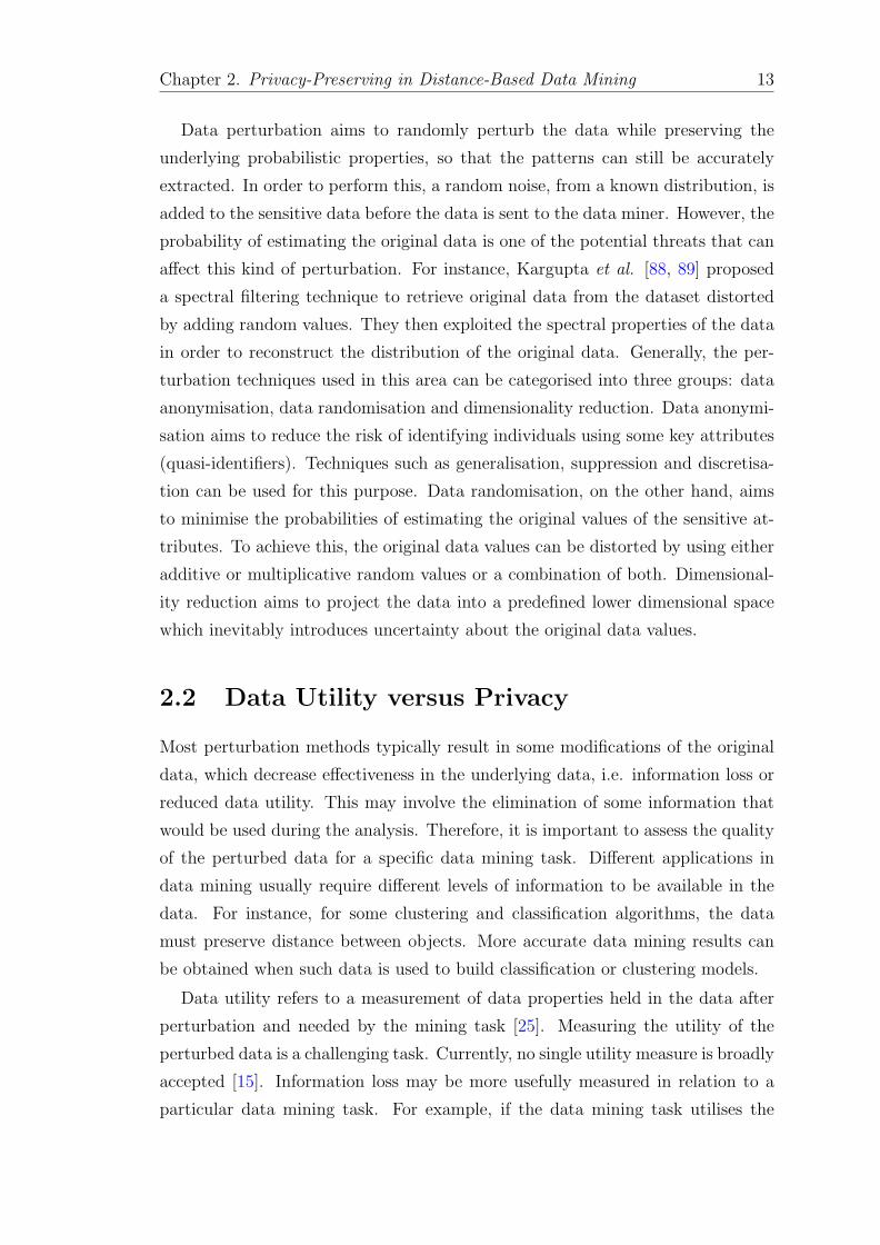
Data perturbation aims to randomly perturb the data while preserving the
underlying probabilistic properties, so that the patterns can still be accurately
extracted. In order to perform this, a random noise, from a known distribution, is
added to the sensitive data before the data is sent to the data miner. However, the
probability of estimating the original data is one of the potential threats that can
affect this kind of perturbation. For instance, Kargupta et al. [88, 89] proposed
a spectral filtering technique to retrieve original data from the dataset distorted
by adding random values. They then exploited the spectral properties of the data
in order to reconstruct the distribution of the original data. Generally, the per-
turbation techniques used in this area can be categorised into three groups: data
anonymisation, data randomisation and dimensionality reduction. Data anonymi-
sation aims to reduce the risk of identifying individuals using some key attributes
(quasi-identifiers). Techniques such as generalisation, suppression and discretisa-
tion can be used for this purpose. Data randomisation, on the other hand, aims
to minimise the probabilities of estimating the original values of the sensitive at-
tributes. To achieve this, the original data values can be distorted by using either
additive or multiplicative random values or a combination of both. Dimensional-
ity reduction aims to project the data into a predefined lower dimensional space
which inevitably introduces uncertainty about the original data values.
2.2 Data Utility versus Privacy
Most perturbation methods typically result in some modifications of the original
data, which decrease effectiveness in the underlying data, i.e. information loss or
reduced data utility. This may involve the elimination of some information that
would be used during the analysis. Therefore, it is important to assess the quality
of the perturbed data for a specific data mining task. Different applications in
data mining usually require different levels of information to be available in the
data. For instance, for some clustering and classification algorithms, the data
must preserve distance between objects. More accurate data mining results can
be obtained when such data is used to build classification or clustering models.
Data utility refers to a measurement of data properties held in the data after
perturbation and needed by the mining task [25]. Measuring the utility of the
perturbed data is a challenging task. Currently, no single utility measure is broadly
accepted [15]. Information loss may be more usefully measured in relation to a
particular data mining task. For example, if the data mining task utilises the
Chapter 2. Privacy-Preserving in Distance-Based Data Mining 14
distance between objects, it would be appropriate to measure how the distance
deviates in the perturbed data. Without specifying which property the analysis is
going to utilise, it is meaningless to make judgement on whether data are “useful”
or “useless”. Hua and Pei [77] argue that data utility in the context of PPDM
is both relative and specific. The term “relative” implies that the utility is an
approximation ratio of how much the perturbed data can preserve some data
properties. The term “specific” implies that the measurement of utility depends
on the specific data mining application such as association rules, classification and
clustering.
Satisfying privacy constraint is one of the most important objective for any
PPDM technique. Although reducing the amount of information can increase the
uncertainty about the original data, the utility of data will decrease. Unfortu-
nately, this tension between privacy and utility is unavoidable. However, these
two concepts should not be compromised in any PPDM algorithm. Indeed, the
ideal perturbation algorithm should minimise both privacy loss and information
loss [28, 109]. However, in practice, finding such an algorithm is difficult as privacy
and utility are typically contradictory in nature. Therefore, preservation of privacy
versus loss of information is always a trade-off in perturbation-based approaches
[72].
2.3 Distance-based Data Mining
The data mining task is an essential process in Knowledge Discovery in Databases
(KDD) where statistical and intelligent approaches are applied in order to extract
useful patterns from data [45]. When considering a set of objects in a multivariate
dataset and given proximity measurements between these objects, the analysis may
concern two situations. The first is examining data to see if some natural groups
or clusters exist. The other is classifying the objects according to a set of existing
groups or classes. Distance-based analysis deals with tools and methods concerning
these two situations. It aims to perform an inference on the available data and
attempts to predict the behaviour of new data instances. Some data mining tasks
utilise the distance between the data objects (e.g. k-NN classification, k-means
clustering, linear discriminant analysis and SVM) so they are known as distance-
based tasks [96]. When the dataset comprises a set of groups and the analysis
requires to find in which group an object should be placed, these tasks generally
use the distance between the objects as a guiding criterion.

Chapter 2. Privacy-Preserving in Distance-Based Data Mining 15
For distance-based clustering, algorithms often measures the distance between
each new object and the centroid, or representative object, of each cluster and
then assigns the new object to the cluster for which its distance to the centroid is
the smallest [160]. The data mining task of clustering is described in Section 5.3.
In general, distance-based clustering consists of two fundamental steps:
1. Defining a proximity measure: Check each pair of objects for the similar-
ity of their values. A proximity measure is defined to measure the closeness
(distance) of the objects. The closer they are, the more similar they are.
2. Grouping objects: On the basis of the distance measures the objects are
assigned to groups so that differences between groups become large and
objects in a group become as close as possible.
For distance-based classification, each object that is mapped to the same class
may be thought of as more similar to the other objects in that class than it is
to the objects found in other classes. Again, proximity measure may be used to
identify the similarity of different objects in the data. Given a test example and
a set of classes, one can compute its distance to the rest of the objects in the
training set and then classify the example according to the class of the majority
of its closest neighbours. For example, in k-NN classification [160], to classify a
new object, the algorithm first finds the k nearest neighbours of that object using
a predefined distance metric. Then, it votes on the class labels of the k nearest
neighbours in order to choose the majority class which is then assigned to the new
object. The k-NN classification is introduced in greater detail in Section 5.3.1.
2.3.1 Distance Measures
Entities in the domain of interest are usually mapped to symbolic representation
by means of some measurement procedure. The relationships between objects are
represented by numerical relationships between variables. Defining a measure is a
crucial process as it underlies all subsequent data analytic and data mining tasks.
Many data mining techniques are based on similarity measures between data ob-
jects, for example, cluster analysis, nearest neighbour classification, and anomaly
detection. There are essentially two ways to obtain measures of similarity. First,
they can be obtained directly from the objects. For example, a marketing sur-
vey may ask respondents to rate pairs of objects according to their similarity.
Alternatively, measures of similarity may be obtained indirectly from vectors of

Chapter 2. Privacy-Preserving in Distance-Based Data Mining 16
measurements or characteristics describing each object. Here, it is necessary to
define precisely what we mean by “similar” so that we can calculate formal simi-
larity measures. Conversely, we can also refer to dissimilarities. When similarities
or dissimilarities are computed, the initial data may no longer be needed as the
analysis can be done on either of them. The term “proximity” is often used as a
general term to denote either a measure (metric) of similarity or dissimilarity [40].
The similarity between two objects is a numerical measure of the degree to
which the two objects are alike. It is non-negative and is often between 0 (no
similarity) and 1 (complete similarity). The dissimilarity between two objects is a
numerical measure of the degree to which the two objects are different. It is also
non-negative and is in the range [0, 1], if it is compared with the similarity, or in
the range [0,∞] otherwise [160]. The term “dissimilarity” is very often used in the
context of data mining to refer to the distance between any two data objects [69].
Once either similarity or dissimilarity has been formally defined, we can easily
define the other by applying a suitable monotonically decreasing transformation.
It is straightforward to transform similarities to dissimilarities and vice versa. For
example, if s(xi, xj) denotes the similarity and d(xi, xj) denotes the dissimilarity
between objects xi and xj, then some transformations may be admissible, e.g.
d(xi, xj) = 1− s(xi, xj), d(xi, xj) = −s(xi, xj), or d(xi, xj) =√
2(1− s(xi, xj)).In practice, data may have variables that are not commensurate and thus the
comparison between data objects may not be fair if this is not taken into account.
For instance, when comparing people based on two variables, say, age and income,
the difference in income will likely be much higher than the difference in age. If
the difference in the ranges of values of age and income are not take into account
during the analysis, then the comparison between people will be dominated by
differences in income. Therefore, to avoid the problem of having a variable with
large values dominate the results of the calculation, we should find some way such
that all variables are regarded as equally important. A common strategy is to
standardise (normalise) the data by dividing each of the variables by its standard
deviation. Let Xk be the kth variable of data X. Two possible techniques for
normalisation can be applied on each value xi of variable Xk. These techniques
are as follows:
1. Min-max normalisation: The variable Xk is scaled so that its values fall
within the range [0, 1], i.e.

Chapter 2. Privacy-Preserving in Distance-Based Data Mining 17
x′i =xi −min(Xk)
max(Xk)−min(Xk), (2.1)
where min(Xk) and max(Xk) are the minimum and the maximum values of
the variable Xk, respectively.
2. Zero-mean normalisation: The values of the variable Xk are transformed
so that Xk has zero mean and unit variance, i.e.
x′i =xi − µkσk
, (2.2)
where µk is the mean (average) of the attribute values and σk is the standard
deviation.
In addition, if we have some idea about the relative importance that should be
assigned to each variable, then we can weight them to yield the weighted distance
measure [41], which can be defined by
δ(xi, xj)w =
n∑k=1
wk δ(xi, xj)
n∑k=1
wk
, (2.3)
where wk is a positive value represents the weight associated with the kth variable
and n is the number of variables.
The weighted distance measure standardises the data only in the direction of
each variable. That means it does not take into account the covariances between
the variables. When some variables are strongly correlated, they may not con-
tribute anything to what we really want to measure. Thus, to eliminate the effect
of redundant variables, one can compute the covariance between all variables. The
covariance of two variables measures their tendency to vary together. It will have
a large positive value if small and large values of one variable tend to be associated
with small and large values of the other variable, respectively. If large values of
one variable tend to be associated with small values of the other, it will take a
negative value. Let µi be the mean of the variable Xi and µj be the mean of the
variable Xj and m be the number of objects. Then the covariance of variable Xi
and variable Xj is defined by
cov(Xi, Xj) =1
m
m∑l=1
(xil − µi)(xjl − µj). (2.4)

Chapter 2. Privacy-Preserving in Distance-Based Data Mining 18
That is, the effect of the correlated variables can be discounted by incorporating
the covariance matrix in the defined distance metric. This leads to the Mahalanobis
distance, which will be defined in Section 2.3.3.1.
The concept of correlation is quite related to the covariance as it also measures
the dependency between two variables. The correlation between two variables Xi
and Xj is defined by
corr(Xi, Xj) =1
σi σjcov(Xi, Xj), (2.5)
where σi and σj are the standard deviation of Xi and Xj, respectively.
The correlation is positive when Xi and Xj have a strong linear relationship
(both increase or decrease together); and negative when Xi and Xj have a weak
linear relationship (one variable increases, the other decreases); and zero when Xi
and Xj are independent, That is, the value of corr(Xi, Xj) is such that −1 ≤corr(Xi, Xj) ≤ 1. Note that if Xi and Xj are standardised, they will each have
a mean of zero and a standard deviation of 1 so that the above formula can be
reduced to the average of the scalar product, i.e.
corr(Xi, Xj) =m∑l=1
xilxjl. (2.6)
If the analysis requires to show how statistically similar all pairs of variables are
in their distributions across the data object, then the inter-correlation coefficients
between objects themselves can be calculated. This is equivalent to thinking of
the objects as columns rather than rows in the data matrix.
2.3.2 Properties of a Distance Metric
The word “distance” relates to a measure of how far or close two quantities are.
It is therefore necessary to consider spaces with some sort of distance that can
be defined on them. Such spaces are known as metric spaces. The metric space
is a set of points with a global function that measures the degree of closeness or
distance of pairs of points in this set [117]. To define a distance metric for a set of
data objects in any n-dimensional space, we should first give a rule, δ(xi, xj), for
measuring closeness (conversely, far-awayness) between any two objects, xi and
xj, in the space. Mathematically, a distance metric is a function, δ, which maps
any two objects, xi and xj, into a real number, such that it satisfies the following
three properties [117]:

Chapter 2. Privacy-Preserving in Distance-Based Data Mining 19
1. δ(xi, xj) is positive definite: If the objects xi and xj are different, the
distance between them must be positive. If the objects are the same, then
the distance must be zero. That is, for any two objects xi and xj, we have
(a) δ(xi, xj) > 0 if and only if xi 6= xj,
(b) δ(xi, xj) = 0 if and only if xi = xj.
2. δ(xi, xj) is symmetric: The distance from xi and xj is the same as the
distance from xj and xi. That is, for any two objects xi and xj, we have
δ(xi, xj) = δ(xj, xi).
3. δ(xi, xj) satisfies triangle inequality: The distance between two objects
can never be more than the sum of their distances from some third object.
That is, for any three objects xi, xj and xk, we have
δ(xi, xk) ≤ δ(xi, xj) + δ(xj, xk).
In other words, the triangle inequality states that if point xi is close to point
xj and xj is close to point xk, xi has to be close to xk as well. This is very
important property when the analysis utilises the distance between objects
since when a predefined metric violates this property, the implicit structure
of similarity between objects may also be violated causing incorrect results.
Measures that satisfy only positivity and symmetry, but not the triangle in-
equality are known as semi-metrics. It is worth noting that the ideal distance
metric should be invariant under admissible data transformations. In other words,
it should be independent of the scale of the data it measures so that more accurate
data mining results can be obtained [151, 176].
2.3.3 Distance Metrics for Numerical, Categorical and
Mixed Data
Often a number of interesting metrics can be defined on a space X; a metric
emphasises some feature of interest while ignoring others. For instance, let X
be a journey from city a to city b. Three possible metrics are dg(a, b), which
measures geographical distance; dc(a, b), which measures travel cost; and dt(a, b),

Chapter 2. Privacy-Preserving in Distance-Based Data Mining 20
which measures travel time. In distance-based data mining tasks, we always mean
the first distance or the distance between real numbers. The most frequently used
and the most natural distance function is the Euclidean distance. It corresponds
to the length of the straight line segment (shortest path) that connects two points.
Given a metric space, one can compute the distance between any two of its
objects, xi and xj. There are many natural ways to measure the distance between
objects in terms of the properties correspond to relationships between values of
their measured variables. The choice of a particular proximity measure often
depends on many factors [64]. However, any chosen metric should capture as
much as possible the essential differences between objects. For instance, to ensure
the consistency and the reliability of the analysis, some factors such as application
of data mining, data distribution and computational complexity would be taken
into consideration when choosing a distance measure.
In this section, various examples of distance metrics are defined since they are
the basis for both non-metric MDS and distance-based data mining. Although it
is easy to show that all metrics we consider in this chapter satisfy the first two
properties (positivity and symmetry) defined in Section 2.3.2, it would be lengthy
to verify the triangle inequality for each metric. The proofs can be found in, e.g.
[122, 138].
2.3.3.1 Dissimilarities Between Numerical Data
The type of proximity measure should fit the type of data [69]. Proximity between
numerical attributes is most often expressed in terms of differences (dissimilarities),
and distance measures provide a well-defined way to quantify such differences into
an overall proximity measure. In this section, we present specific examples of some
dissimilarity measures that are widely used with numerical data.
• Minkowski Distance
The general form of the Euclidean distance is the Minkowski distance. Con-
sider two points, xi and xj, in n-dimensional space, X, the Minkowski dis-
tance is defined by
d(xi, xj) =
(n∑k=1
|xik − xjk|r)1/r
, (2.7)
where r is a positive parameter and xik and xjk are the kth attributes of xi
and xj, respectively.

Chapter 2. Privacy-Preserving in Distance-Based Data Mining 21
• Manhattan Distance
When r = 1, the Minkowski distance is called Manhattan distance (L1 norm).
The distance between two points, xi and xj, is the sum of the absolute
differences of their coordinates; and measured along axes at right angles.
For example, the distance between two points, xi at coordinates (xi1, xi2)
and xj at coordinates (xj1, xj2) in R2, is |xi1− xj1|+ |xi2− xj2|. This metric
is also known as city-block and it can be defined by
d(xi, xj) =n∑k=1
|xik − xjk|. (2.8)
This is obviously equivalent to the Hamming distance [68], which is the
number of coefficients in which two objects that have only binary attributes
differ.
• Euclidean Distance
When r = 2, the Minkowski distance is known as Euclidean distance (L2
norm). The Euclidean distance between two points, xi and xj, is defined by
d(xi, xj) =
(n∑k=1
|xik − xjk|2)1/2
. (2.9)
That is, it is equal to the square root of the sum of the intra-dimensional
differences, xik−xjk, which is simply the Pythagorean theorem for the length
of the hypotenuse of a right triangle.
• Max Distance
When r =∞, the Minkowski distance is known as Max distance (L∞ norm),
which is defined by
d(xi, xj) =n
maxk=1|xik − xjk|. (2.10)
This metric, like Manhattan Distance, examines the absolute magnitude
of the element-wise differences, xik − xjk, in the pair of vectors for two
objects and chooses the largest one. Thus, it is equal to the maximum
of the differences.
Figure 2.2 shows various proximity contours for the case where point xi is
fixed at the origin, (0, 0), and point xj is moved to different position in the

Chapter 2. Privacy-Preserving in Distance-Based Data Mining 22
−3 −2 −1 0 1 2 3−3
−2
−1
0
1
2
3
(a) Manhattan
−3 −2 −1 0 1 2 3−3
−2
−1
0
1
2
3
(b) Euclidean
−3 −2 −1 0 1 2 3−3
−2
−1
0
1
2
3
(c) Max
Figure 2.2: Contour plot of the neighbourhood for a point at the origin (0, 0)using different distance measures. Contour lines close to (0, 0) have low values,
whereas further away lines have higher values.
space. The contour lines show the set of positions where xj has the same
proximity to xi. Each distance has its own isosimilarity shape, which is the
curve representing the set of all points (neighbourhood) with same distance
to the point at origin, i.e. xi. The isosimilarity curve looks like a diamond,
circle and square for the case when r = 1, r = 2 and r =∞, respectively.
Example 2.1. Let x1 = (2, 3, 1) and x2 = (0, 1, 2). Then,
the Manhattan distance is
d(x1, x2) =n∑k=1
|x1k − x2k| = |2− 0|+ |3− 1|+ |1− 2| = 5,
the Euclidean distance is
d(x1, x2) =
(n∑k=1
|x1k − x2k|2)1/2
=√
(2− 0)2 + (3− 1)2 + (1− 2)2 = 3,
the Max distance is
d(x1, x2) =n
maxk=1|x1k − x2k| = max(|2− 0|, |3− 1|, |1− 2|) = 2,
• Mahalanobis distance
Sometimes it is worth taking into account the correlations of the attributes
when measuring the distance between objects. For this purpose, the Maha-
lanobis distance is suggested. The Mahalanobis distance is mathematically
defined by

Chapter 2. Privacy-Preserving in Distance-Based Data Mining 23
−3 −2 −1 0 1 2 3−3
−2
−1
0
1
2
3
2
4
6
8
10
12
14
16
18
20XY
Figure 2.3: Mahalanobis distances between the points represented by squaresand the remaining points represented by circles. The colour bar represents howfar the points represented by squares are from the points represented by circles.
The more blue is the colour the closer is the point.
d(xi, xj) =
((xi − xj) Σ−1 (xi − xj)T
)1/2
, (2.11)
where Σ−1 is the inverse of the covariance matrix of the data.
It can be seen that since Σ is a non-singular covariance matrix, it is positive-
definite and hence d(xi, xj) is a metric. The Mahalanobis distance is analyti-
cally preferred to other metrics when attributes are correlated, have different
variance, and the data has normal distribution [160]. Figure 2.3 shows an
example of calculating the Mahalanobis distance between some points with
two variables, X and Y . The points in Y with equal coordinate values are
much closer to X than points with opposite coordinate values, even though
all points are approximately equidistant from the mean of X in Euclidean
distance. This indeed implies that the isosimilarity curve of the neighbour-
hood in the Mahalanobis distance takes an elliptical shape.
Example 2.2. Table 2.1 shows five data objects in 2-dimensional space, X. The
Mahalanobis distances between these objects and the objects y1 = (1, 2), y2 =
(2, 2), and y3 = (−1, 0) are shown in Table 2.2. Since the object y1 is close to the
mean of the data X, it has a low Mahalanobis distance (d(y1, X) = 2.2) compared
with other objects y2 and y3.

Chapter 2. Privacy-Preserving in Distance-Based Data Mining 24
Table 2.1: An example of five data objects in 2-dimensional space.
Object X1 X2
x1 0 1x2 2 1x3 1 1x4 -1 2x5 1 -1
Mean 0.6 0.8
Table 2.2: Mahalanobis distance between the data objects in data X and theobjects y1, y2 and y3.
Object Y1 Y2 d(yi, X)
y1 1 2 2.2y2 2 2 5.2y3 -1 0 4.5
2.3.3.2 Similarities of Categorical Data
The notion of “similarity” is often used with data that contains categorical at-
tributes and thus it is sometimes called similarity coefficient. The similarity be-
tween two objects is related to the differences between them. The more differences
they have, the less similar they are. If s(xi, xj) is the similarity between two objects
xi and xj, then s(xi, xj) typically has the following properties:
1. s(xi, xj) is positive definite, i.e.
s(xi, xj) =
1 if and only ifxi = xj,
0 otherwise.
This implies that when s(xi, xj) equals 1 the two objects, xi and xj, are
completely similar, whereas when s(xi, xj) equals 0 the objects xi and xj are
different.
2. s(xi, xj) is symmetric, i.e.
s(xi, xj) = s(xj, xi) for all xi and xj.
For most similarity measures, the triangle inequality typically may not hold
and thus they cannot be a metric [64, 166]. However, it is easy to convert any
non-metric similarity measure to a metric distance as described above in Section

Chapter 2. Privacy-Preserving in Distance-Based Data Mining 25
2.3.1. For instance, a simple similarity measure, s(xi, xj) = 1 when xi and xj are
equal, and s(xi, xj) = 0 otherwise, does not satisfy the triangle inequality, but
s′(xi, xj) =√
1− s(xi, xj) does and thus s′(xi, xj) is a metric and equivalent to
the Euclidean distance.
To measure the distance between two objects with categorical attributes, it is
natural to construct a so-called contingency table, which contains in its cells the
frequencies with which two attributes were sorted into the same group. Let xil
and xjl be two attributes of interest in the objects xi and xj, respectively. Let
z = f(xil, xjl) be the frequency of an event (xil, xjl). In particular, let a = f(0, 0)
be the frequency of the event where both xil and xjl are absent, b = f(0, 1) be
the frequency of the event where xil is absent and xjl is present, c = f(1, 0) be
the frequency of the event where xil is present and xjl is absent, and d = f(1, 1)
be the frequency of the event where both xil and xjl are present. Some possible
similarity measures are defined as follows:
• Simple matching coefficient
s(xi, xj) =a+ d
a+ b+ c+ d. (2.12)
• Jaccard coefficient
s(xi, xj) =d
b+ c+ d. (2.13)
• Hamman coefficient
s(xi, xj) =(a+ d)− (b+ c)
a+ b+ c+ d. (2.14)
• Cosine similarity
s(xi,xj) =xi.xj
||xi|| ||xj||, (2.15)
where xi and xj are two vectors each of which has n elements and each ele-
ment contains the frequency that a predefined event is present. The notation
“.” denotes the dot product and ||.|| is the length of the vector.
The cosine similarity indeed is a measure of the cosine of the angle between xi
and xj. Thus, the smaller the angle, the more similar are the two vectors.
Chapter 2. Privacy-Preserving in Distance-Based Data Mining 26
Similarity measures are generally distinguished according to whether or not the
0-0 matching, i.e. a = f(0, 0), is included to the measure’s formula. Many various
similarity measures are proposed in the literature (see, e.g, [81] for a comprehensive
list of similarity measures). Nevertheless, the particular choice of which to use
depends on the application. For instance, if the analysis requires to calculate the
similarity between two documents where each document is represented as a vector
and each attribute contains the frequency with which a particular word occurs
in the document, then the most common and appropriate measure is the cosine
similarity [44].
Example 2.3. Let x1 = (1, 0, 0, 0, 0, 0, 0, 0, 0, 0) and x2 = (0, 0, 0, 0, 0, 0, 1, 0, 0, 1).
Then we have
s(x1, x2) =a+ d
a+ b+ c+ d=
7 + 0
7 + 2 + 1 + 0= 0.7,
for the simple matching coefficient, and
s(x1, x2) =d
b+ c+ d=
0
2 + 1 + 0= 0,
for the Jaccard coefficient, and
s(x1, x2) =(a+ d)− (b+ c)
a+ b+ c+ d=
(7 + 0)− (2 + 1)
7 + 2 + 1 + 0= 0.4,
for the Hamman coefficient, and
s(x1, x2) =xi.xj
||xi|| ||xj||=
0
1× 1.41= 0,
for the cosine similarity.
2.3.3.3 Similarities of Mixed Data
In real world, the data often contains objects with attributes of mixed data type.
Therefore, to guarantee the quality of comparing objects, one may calculate the
distance by combining the methods mentioned in the above previous sections (Sec-
tion 2.3.3.1 and 2.3.3.2). For instance, when calculating the distance between ob-
jects, xi and xj, using the Euclidean distance, one may calculate the difference
between nominal and binary attributes as 0 or 1, i.e. “match” or “mismatch”,
respectively. Similarly, the difference between numeric attributes as the squared
difference between their normalised values. That is, the total distance is obtained

Chapter 2. Privacy-Preserving in Distance-Based Data Mining 27
by taking the summation over each difference. Note that it would be easy to
transform some categorical values, for example “low”, “medium” and “high”, into
numeric values, and thus deal with the data using one numeric metric. However,
when the categorical attributes contain unordered values like “red”, “green” and
“blue”, the transformation would be challenging since these kind of attributes
cannot be ordered naturally, and hence we cannot assign them numerical values.
Let xi and xj be two data objects that have attributes with mixed data types
(numerical and categorical), the similarity measure [78, 79] between them can be
introduced as follows:
s(xi, xj) =
(n∑k=1
|xik − xjk|2)1/2
+ wk
c∑k=1
δ(xik, xjk), (2.16)
where the first term is the Euclidean distance measured on the n numerical at-
tributes and the second term is the weighted simple matching similarity measured
on the c categorical attributes and wk is the weight associated with the kth cate-
gorical attribute.
Alternative similarity measure for mixed data was proposed by Grower [63] as
follows:
s(xi, xj) =
n∑k=1
wk δ(xik, xjk)
n∑k=1
wk
, (2.17)
where δ(xik, xjk) is the similarity between the kth variable of the objects xi and
xj and wk is the associated weight, which equals to one if the two objects xi
and xj can be compared on the kth variable and equals zero otherwise. If the
kth variable is categorical, then the similarity, δ(xik, xjk), is defined as a simple
matching coefficient. Whereas if the kth variable is numerical, then δ(xik, xjk) is
defined as δ(xik, xjk) = 1 − |xik − xjk|/max(Xk) − min(Xk), where max(Xk) −min(Xk) represents the range of the values for the kth variable, Xk. This definition
ensures that 0 ≤ δ(xik, xjk) ≤ 1 for all xi and xj.
Once the similarities are calculated, the data mining algorithm can work on
them in order to minimise the cost function associated with the mining task. For
example, in each iteration of the k-means clustering algorithm, each data object
can be assigned to its nearest cluster centre according to one of the similarity
metrics defined above. Then the cluster centres are re-calculated as the mean of
all the objects belonging to that cluster [9].
Chapter 2. Privacy-Preserving in Distance-Based Data Mining 28
2.3.4 Distance-Based Tasks
The main distance-based tasks in data mining are briefly described as follows:
• Classification and Prediction
The classification problem is described as assigning objects to one of sev-
eral predefined categories. For example, a patient data may have a class
attribute called Diagnosis along with several other attributes that describe
various properties and conditions of a patient. Given a set of patients, one
can classify each individual into separate and distinct categories that allow
medical decisions about treatment to be made. The input data for classifi-
cation is a collection of objects (also known as instances or examples) each
of which is characterised by a tuple (x1, x2, . . . , xn, ci), where xi is non-class
attribute and ci is the class attribute (also known as label or target attribute).
The non-class attribute set may include data from different types while the
class attributes is often discrete. Classification is the task of learning a target
function f that maps each attribute set, x1, x2, . . . , xn, to one of predefined
class label, ci. It discovers a pattern (model) that explains the relationship
between the class and the non-class attributes [160].
The classification model is often used as either descriptive or predictive.
In the former, the classification model can serve as an explanatory tool to
distinguish between objects of different classes, whereas the later aims to
use the classification model to predict the class label of unlabelled objects.
The predictive modelling involves two steps: (1) an inductive step where
the classification model is constructed from the training dataset, and (2) a
deductive step where the model is applied to the testing dataset. When the
classification algorithm optimises a distance function in order to build the
model, then classification is a distance-based task. An example of distance-
based classification is the k-NN algorithm, which classifies the new test object
based on the class label of its neighbours. In the case where the neighbours
have more than one label, the object is assigned to the majority class of its
neighbours. The classification model is sometimes called classifier, which
can be expressed in different ways such as decision tree, rule-based classifier,
neural network, support vector machine or naıve Bayes classifier.

Chapter 2. Privacy-Preserving in Distance-Based Data Mining 29
• Clustering
Clustering is the process of arranging similar objects in groups so that the
objects belonging to the same cluster have high similarity, while objects
belonging to different clusters are well separated [69]. Unlike classification,
clustering does not rely on predefined classes but rather derives the class label
from the data so that it is sometimes referred to as unsupervised learning.
Typical applications of clustering include discovery of medicine and genes,
identification of loyal customers, risk analysis, detection of banking fraud
and many other applications [57].
The major clustering methods can be classified into the following categories
[67]:
– Partitioning Clustering: This method generally divides m data ob-
jects into k non-overlapping and mutually exclusive subsets (clusters),
where k is a specified number and k ≤ m. The method then iteratively
improves the quality of the partitions by grouping similar objects, in
terms of their distances to the representative object or centroid. Var-
ious kinds of criteria can be used for judging the quality of partitions
[67]. The most common algorithms used for partitioning clustering are
k-means [73], PAM [91] and CLARANS [125].
– Hierarchical Clustering: These methods arrange a set of objects in
a hierarchy with a tree-like structure based on the distance or similarity
between the objects. In general, they are classified into two categories—
agglomerative and divisive. The agglomerative approach begins with
each object placed in a separate cluster. Then the distance between all
possible combinations of two objects is calculated using a selected dis-
tance measure. The two most similar clusters are then grouped together
and form a new cluster. In subsequent steps, the distance between the
new cluster and all remaining clusters is recalculated. Clusters are
merged until only one cluster remains. On the other hand, the divisive
approach starts with all objects in a single cluster and then splits a
cluster into two clusters such that the quality of the overall clustering
is improved. The algorithm stops when a termination condition is met
or each object is assigned into a different cluster.
– Density-Based Clustering: This method typically locates regions
of high density that are separated from one another by regions of low
Chapter 2. Privacy-Preserving in Distance-Based Data Mining 30
density. DBSCAN [55] is well-known algorithm of this category. The
algorithm searches for clusters by checking the neighbourhood of each
object in the data. Given input parameters such as neighbourhood
radius, ε, and minimum number of objects, MinPts, each object x is
examined to determine whether or not its neighbourhood contains at
least MinPts objects. If this condition is satisfied, then a new cluster
with x as a core object is created. The algorithm then iteratively collects
directly density-reachable objects from these core objects, which may
involve the merge of a few density-reachable clusters. The algorithm
terminates when no new object can be added to any cluster.
– Grid-Based Clustering: These methods perform all clustering oper-
ations on a grid-like structure obtained by quantising the data space
into a finite number of cells. The main advantage of these methods is
their fast processing time since they mainly depend only on the num-
ber of cells in each dimension in the quantised space. STING [177] is a
typical example of a grid-based clustering in spatial databases.
– Fuzzy Clustering: These methods allow the objects to belong to sev-
eral clusters at the same time, with different degrees of membership.
Intuitively, fuzzy clustering is more natural than hard (crisp) cluster-
ing because objects on the boundaries between several clusters are not
forced to fully belong to one of the clusters but rather are given a mem-
bership degree between 0 and 1 indicating their partial membership. A
common algorithm for fuzzy clustering is FCM [16].
2.3.5 Neighbourhood Space of an Object
In order to guarantee the correctness of data analysis of perturbed data, partic-
ularly in the context of distance-based data mining, the neighbourhood relations
between objects in the perturbed space should be accurately measured. Indeed,
preserving neighbourhood’s relations in the mapping may help to discover the
hidden structures (groups and clusters) underlying the original data [14].
A distance metric is a function of two variables on a set X, i.e. a function of
the Cartesian product, X ×X, of X with itself, which is non-negative, symmetric
and satisfies the triangle inequality [117]. Given a set X, one can define an open
ball or radius r > 0 around a point x ∈ X as the set of all points at a distance less
that r from x. The neighbourhood space of point x is the set of all points, N , such

Chapter 2. Privacy-Preserving in Distance-Based Data Mining 31
that each point in N is within a specified distance, r, from x. Mathematically, it
is defined as follows:
Definition 2.1 (Neighbourhood space). In a metric space (X, d), a set N is a
neighbourhood of a point p if there exists an open ball with centre p and radius
r > 0, such that N = {x ∈ X : d(x, p) ≤ r}.
The elements in N are called the nearest neighbours of p with respect to the
distance r and the metric d. The parameter r is the radius of the neighbourhood
space. The set of points B satisfying d(p,B) = r, is called the boundary of the
neighbourhood.
As mentioned earlier in Section 2.3.3, different distance metrics result in neigh-
bourhoods with different sizes and different shapes. For instance, the neighbour-
hood of point x, in a two dimensional space, using Manhattan distance metric is
a diamond. The centre of the neighbourhood is the intersection point of its diago-
nals. The length of each side of the diamond is√
2r and each side makes angle of
45 ◦ with the axes and the length of the diagonals is 2r. For Euclidean distance,
the neighbourhood space is a circle with radius r and centre x; the centre of the
circle is the centre of the neighbourhood. For Max distance, the neighbourhood is
a square with sides 2r and centre x. The sides of the square are paralleled to the
axes.
2.3.6 Decision Boundaries for Distance Metrics
The decision boundary between two classes is a hyperplane that partitions the
underlying data space into two sets, one for each class, so that the classifier can
assign all the objects on one side of the decision boundary to one class and all
those on the other side to the other class. To illustrate this, consider the following
example. Let a and b be two points in 2-dimensional space, where each point
belongs to a distinct class, ci, and let x be a moving point in the space (see
Figure 2.4(a)). All possible locations of the point x that satisfy the condition
d(x, a) = d(x, b) form a hyperplane H (a line in a 2-dimensional space), which
divides the space into two half planes. The points in the half plane R1 are closer
to the point a; the points in the half plane R2 are closer to the point b and the
points on the hyperplane H have the same distance from a and b. This hyperplane
H is called the decision boundary between the two classes for the metric d. The
regions R1 and R2 are called decision regions of the predefined classes c1 and c2,
respectively.

Chapter 2. Privacy-Preserving in Distance-Based Data Mining 32
d(x,b)
d(x,a)R2 R1
x
a
b
H
DecsionBoundary
(a) Linear case
R1
R2
(b) Non-linear case
Figure 2.4: An example of the decision boundary between two classes (blueand red) for linear data (a) and non-linear data (b). The hyperplane H is theoptimal decision boundary that separates the two classes. The region R1 denotesthat part of input space classified as blue, while the region R2 is classified as
red.
The distance measure, d, determines the geometry of the decision boundary. For
example, when d is Euclidean distance, the hyperplane, H, is the perpendicular
bisector to the line segment matching the points a and b. When d is Manhattan
distance, H is a 3-segment line such that the middle segment is a straight line of
45 ◦ with the x-axis and the other two segments are parallel to the y-axis. When
d is Max distance, H is also a 3-segment line such that the middle segment is
parallel to the y-axis and the other two segments are a straight lines of 45 ◦ with
the x-axis.
However, data, in most real cases, are non-linear, i.e. classes are not linearly
separable and may possibly have discontinuous decision boundaries, and thus a
linear decision boundary is unlikely to be optimal. In such cases, the optimal
decision boundary is non-linear, disjoint and more difficult to obtain [74]. Figure
2.4(b) shows an example of a non-linear decision boundary.
In distance-based learning, the algorithm attempts to assign unseen objects
to the closest group under the guidance of a predefined distance measure. The
performance of the algorithm often depends on the underlying topological struc-
ture of the data, i.e. data distribution or the relationship between a point and
its neighbours. Therefore, it is important for any PPDM transformation to pre-
serve as far as possible the essential topology of the original data such that nearby
and far away points in the original space are mapped into nearby and far away
points, respectively, in the transformed space. When the underlying structure of

Chapter 2. Privacy-Preserving in Distance-Based Data Mining 33
the data is well preserved, the decision boundaries are likely to remain unchanged
[75, 103]. This propriety is very important for many distance-based algorithms
particularly those seeking a hyperplane that separates the feature space into a set
of classes with a maximum margin. For instance, SVM [36] employs optimisa-
tion functions to find optimal boundaries between classes such that the optimal
boundaries should generalise to unseen samples with least errors among all pos-
sible boundaries separating the classes. In other words, it maximises the margin
between the classes on the training data and thus better classification performance
on test data can be obtained.
2.3.7 Transformation-Invariant Data Mining
The utility of the data can be measured in two ways either by quantifying in-
formation loss incurred by the transformation process or by assessing how well
the transformed data support a certain data mining task. Since the distance are
most important in the analysis, one can measure the size of distance deviation in
the original and the transformed spaces. This gives how much information is lost
during the transformation. Alternatively, one can evaluate the accuracy of results
obtained from the original and the transformed data. For instance, if the task
is classification, the accuracy of the classifier on both the original data and the
transformed version can be used as a measure for data utility.
Data perturbation can be seen as a transformation from the original space to
the perturbed space. When the data mining results obtained from the original
and the perturbed data are similar, one can say that the data mining algorithm
that operated on both of them is invariant under the transformation. However,
since most transformation methods typically downgrade some properties required
by the analysis, the term “invariant” would be better understood as maintaining
as small a discrepancy as possible. Let acc(X) and acc(T (X)) be the accuracies
obtained by an algorithm A on the original data, X, and the transformed data,
T (X), respectively. The transformation-invariant algorithm is defined as follows:
Definition 2.2 (Invariant data mining algorithm). A data mining algorithm A is
invariant to a transformation T if and only if acc(X)− acc(T (X)) ≤ e, where e is
a small value such that 0 ≤ e ≤ 1.
This implies that perturbation should be performed so the data analysis on the
perturbed data yields conclusions that are invariant with the conclusions derived
from the original data. That is, replacing an object x by an object T (x) does not

Chapter 2. Privacy-Preserving in Distance-Based Data Mining 34
change the accuracy of data mining algorithm. If acc(X) − acc(T (X)) = 0, then
the algorithm is strictly invariant to the transformation.
As we will see in Chapter 3, non-metric MDS usually aims at preserving both
the Euclidean distance and the underlying data structure with small error. The
overall group topology approximately remains unchanged before and after the
perturbation [42]. Therefore, any distance-based algorithm should be able to de-
termine the right group membership for each data object and thus invariant results
can be obtained.
2.4 Data Anonymisation Methods
Published data may violate individual privacy when one can easily identify a single
record from a set of data records. The anonymisation methods aim to mask the
detailed information of any sensitive attributes and minimise the probability of
re-identifying the record owner. The sensitive attributes are those that contain
confidential or private information as pre-specified by the data owner.
In the area of data publishing, many methods of data anonymisation have been
developed in order to prevent the re-identification of individual identities. The
k-anonymisation method [158] guarantees privacy by ensuring that any record in
a published dataset be indistinguishable from at least (k− 1) other records in the
data. The re-identification of a given record usually depends on a set of attributes
known as quasi-identifiers which are non-sensitive attributes but could potentially
uniquely identify record owners [60]. Thus, in the k-anonymity model, the risk of
re-identification is maintained under an acceptable probability, i.e. 1/k [119]. One
drawback of k-anonymisation is that the distribution of some quasi-attributes may
be lost as a result of the generalisation process. For instance, an attribute, let’s
say Age, can be generalised to a set of domain intervals, and therefore, the specific
distribution information of this attribute is lost. To overcome this problem, Kifer
and Gehrke [94] proposed a technique to inject additional information into the
k-anonymous tables using marginal tables. The marginal table of any generalised
attribute is a simple count of all tuples sharing the same value in the original
domain of that attribute.
Despite the effectiveness and simplicity of implementing the k-anonymisation,
it is vulnerable to different kinds of attacks such as record linkage and attribute
linkage. Record linkage [173] can occur when the attacker is able to link a record
owner to a record in the anonymised data, whereas, attribute linkage [31] can occur

Chapter 2. Privacy-Preserving in Distance-Based Data Mining 35
when the attacker is able to link a record owner to a sensitive attribute. There-
fore, the technique of `-diversity [113] was proposed which not only maintains the
minimum group size of k records, but also maintains the diversity of the sensitive
attributes. This model would provide a stronger protection against attacks since
the larger the value of `, the more difficult it becomes to discover the possible
values of the sensitive attribute. However, in some cases, the sensitive values are
naturally more frequent than others in a single group. Therefore, the `-diversity
model may fail to prevent probabilistic inference attacks [2].
In [8], a further enhancement for k-anonymisation and `-diversity was suggested.
This method randomly chooses whether to keep or replace each record in the
anonymised data with another record, randomly chosen from the domain of all
variables in such a way that the proportion of retained records is no less than a
predefined threshold. However, it has been shown in [134] that all theses data
anonymisation methods are often subject to low privacy and low utility. The
t-closeness model [102] is a further enhancement of the `-diversity model. This
model requires that the distribution of a sensitive attribute in any equivalence
class is close to the overall distribution of the attribute in the data, i.e. the
distance between the two distributions should be no more than a threshold t. The
equivalence class is simply defined as a set of records that have the same values for
quasi-identifiers [32]. Aggarwal and Yu [2] argue the t-closeness approach would
provide a more effective solution than many other PPDM methods particularly
when the sensitive attribute is numeric. However, Domingo-Ferrer and Torra [49]
criticise this model since enforcing t-closeness may minimise the data utility, and
thereby affect the discovery of data patterns.
Due to the limitation of data anonymisation methods in preserving most of data
properties such as distances between data points, data distribution and granularity
of data, they are not effective for most data mining applications since, in practice,
most data mining techniques are highly dependent on these data properties.
2.5 Data Randomisation Methods
Data randomisation is one of the traditional techniques used for protecting the
private information of individuals in statistical databases (SDB) whilst maintain-
ing the statistical properties [95, 104, 164]. Data randomisation methods attempt
to disguise the sensitive data by randomly modifying the data values often using
either additive noise or multiplicative noise or a combination of these two methods
Chapter 2. Privacy-Preserving in Distance-Based Data Mining 36
all together. In fact, the size of the noise added to an individual value gives an in-
dication of how difficult it is to recover the original value. Thus, using sufficiently
high levels of noise may provide good privacy protection.
In the additive perturbation [7, 111], random numbers drawn from a normal
distribution with zero mean, µ = 0, and standard deviation σ are added to the
original data values. In contrast, in the multiplicative perturbation, the original
data points are either projected to a randomly chosen lower-dimensional space
[110, 129] or rotated using an orthogonal transformation [24]. In [27, 28], an
enhancement of rotation perturbation was suggested where extra components are
added to the perturbation model including translation matrix and noise addition.
Kenthapadi et al. [92] propose a privacy model using both projection and additive
perturbation.
One of the unique features that distinguishes rotation perturbations from other
perturbations is that it provides good data utility for some data mining tasks,
including classification and clustering. Since many data mining models utilise
Euclidean distance or inner product, as long as such information is preserved,
models trained on perturbed data will have similar accuracy to those trained on the
original data [24]. However, in projection perturbation, the pairwise distances are
not strictly preserved but rather maintained with some distortion, and therefore,
the accuracy of a data mining model may still be negatively affected.
Despite the fact that multiplicative perturbations preserve some data proper-
ties, they may not provide effective protection for private data. Liu et al. [110]
argue that if the original data vectors are statistically independent and do not
follow a Gaussian distribution, it is possible to estimate their original forms quite
accurately. Liu et al. [108] also proposed a PCA-based attack by which the at-
tacker can use prior knowledge to estimate the original data from the perturbed
data. Similarly, Turgay et al. [165] proposed a similar PCA-based attack but
with different assumptions. Guo and Wu [66] proposed a method that is based
on Independent Component Analysis (ICA) to derive the original from the per-
turbed data. However, the ICA approach is not efficient because the order of the
independent components of the original data cannot be determined and the vari-
ance of the original data signals cannot be preserved even though the order of the
independent components can be successfully determined [28, 127].

Chapter 2. Privacy-Preserving in Distance-Based Data Mining 37
2.6 Dimensionality Reduction for Privacy-Pre-
serving Data Mining
Methods of dimensionality reduction provide a way to understand and visualize
the structure of complex data. Recently, they have been proposed for ensuring
that a given data, in a lower space, are protected against privacy threats, and
meanwhile expose many of the useful and interesting properties of the original data.
Dimensionality reduction methods assume that the data records are represented
as vectors in a multidimensional space where each dimension represents a single
attribute. The entire database is represented as an m× n matrix with m records
and n attributes. In general, these methods aim to map each data object in the
high dimensional space, Rn, into a point in the lower dimensional space, Rp such
that a distinct property of data is maintained, i.e. T : X → Y where X is the
original data and Y is the perturbed data. The basic problem inherent in these
type of mapping is that they usually result in some distortion of the data being
mapped. It is very rare to find a mapping between two spaces of interest in which
distances are exactly preserved, and hence, we often have to allow the mapping to
alter the distances in some fashion but hopefully with restricted damages as much
as possible. This section presents a brief summary and review of dimensionality
reduction methods used for PPDM and comments on their characteristics.
2.6.1 Random Projection Perturbation
Random Projection (RP) aims to protect the original data values, whilst preserving
the data utility, by projecting data objects in n-dimensional space into a lower p-
dimensional space, where p < n, capturing as much of the variation of the data as
possible. The RP can be defined by
Y = XR, (2.18)
where R is an n×p RP matrix onto p-subspace such that each column is orthogonal
and the elements rij have zero mean and unit variance [129]. Let A be a matrix
whose columns are linearly independent vectors, then the projection of matrix X
into the subspace of the columns of A is known to be R = A(ATA)−1AT [118].
Note that even though A still embeds X into the lower dimensional space, it is no
longer an isometry in general.

Chapter 2. Privacy-Preserving in Distance-Based Data Mining 38
This approach is fundamentally based on the result of Johnson-Lindenstrauss
lemma [85] which says that any n points subset of Euclidean space can be embed-
ded into a random subspace of p = O(log n/ε2) dimensions without distorting the
pairwise distances by more than a factor of (1 ± ε), for any 0 < ε < 1. This im-
plies that there is a transformation T : Rn → Rp such that the distances between
the points are approximately preserved. Let x and y be two points in the higher
dimension, Rn, T (x) and T (y) be their images in the lower dimension, Rp, there
exists ε > 0 such that the distance between x and y and their images T (x) and
T (y) is bounded by
(1− ε)||x− y|| ≤ ||T (x)− T (y)|| ≤ (1 + ε)||x− y||. (2.19)
By using such a transformation, it would be possible to change the original form
of data whilst maintaining the distance properties by a small error ε. However,
since the pairwise distances are not strictly preserved but rather maintained with
some distortion ε, the accuracy of data mining model may still be negatively
affected. Assume that data points of the original data are represented as column
vectors in matrix X, i.e. X is an n×m matrix, Liu and Kargupta [110] define a
perturbation model that preserves the inner product as
Y =1√pσ
XR, (2.20)
where each entry rij of R is independent and identically distributed chosen from
a distribution with mean µ = 0 and standard deviation σ. It has been proved
in [107] that E[RTR] = nσ2I, where n is the number of rows of matrix R, and
I is the identity matrix. The values of the original data X can be estimated
as E[Y TY ] = XTX since the entries of the random matrix are independent and
identically distributed.
2.6.2 PCA-based Perturbation
Principal Component Analysis (PCA) is a linear transformation method which
aims to find a lower subspace that preserves much of the variance. It seeks new
uncorrelated features that explain most of the total variance of data, and thus
reject noisy features that account for low variance. Let Σ = 1n−1
XTX be the
covariance matrix of the original data. The matrix Σ can be decomposed as
UΛUT where U is an m× n matrix containing the eigenvectors corresponding to
Chapter 2. Privacy-Preserving in Distance-Based Data Mining 39
eigenvalues of Σ and Λ is an n × n diagonal matrix containing the eigenvalues,
λ1, λ2, . . . , λn. Without loss of generality, the eigenvalues of Σ can be ordered in
a non-increasing order, λ1 ≥ λ2 ≥ . . . ≥ λn, thus the columns of Y have also
non-increasing variances. To project the data to a p-dimensional space, we keep
the first p columns in U that count for most of the variance and discard the rest
of the columns. The perturbed data Y can then be generated by
Y = XUp.
The subspace, Y , spanned by the first p eigenvectors has the smallest sum
of squared Euclidean distances’ deviation from the original space X. In other
words, the “best-fit” that minimizes the distortion of distances in the subspace,
Y , is determined by the first principle components [86]. Banu and Nagaveni [11]
proposed a PCA-based approach to perturb the data using a set of samples that
are randomly drawn from the original data but no rigorous analysis of privacy
preservation was given. Later they generalised their approach for a multi-party
clustering scenario [174].
2.6.3 SVD-based Perturbation
Single Value Decomposition (SVD) is quite close to PCA because the idea of
eigenvalue decomposition can be generalized to an arbitrary (non-symmetric, non-
square) matrix X. The matrix X can be factorized into USV T where U is an
m × n orthogonal matrix containing the eigenvectors of XXT and S is an n × ndiagonal matrix containing the singular values, σ1, σ2, . . . , σn and V is an n × northogonal matrix containing the eigenvectors of XTX. Each σi is equal to
√λi,
the square root of the eigenvalues of Σ. Similarly, we can order singular values in
decreasing order of magnitude, σ1 ≥ σ2 ≥ . . . ≥ σn and retain the p eigenvectors
that capture the maximum variation; and project the data into the p-dimensional
space to generate the perturbed data Y , i.e.
Y = USpVT .
Note that the smallest singular values are often considered to be due to noise,
and thus removing them will not affect the difference of Euclidean distances be-
tween the original data, X, and the perturbed data, Y . Xu et al. [178] used SVD
to transform the data to a lower dimension and then, to enhance the privacy, they
Chapter 2. Privacy-Preserving in Distance-Based Data Mining 40
modified some entries of the matrix U and V that are less than a pre-specified
threshold. A similar approach was suggested in [101] to perturb different sam-
ples of data using different setting of the pre-specified threshold. However, the
modification of some entries values causes much loss of information and heavily
distorts the distances between the data points as the dimensionality decreases.
This would affect the data analysis and lead to poor data mining results as we
will see in Chapter 5. Lin et al. [105] proposed a method that first reduces the
dimensionality of the original data using a filter-based feature selection method
and then distorts the selected subset using SVD. Lakshmi and Rani [99] used a
combination of SVD and random multiplication to generate the perturbed data.
2.6.4 Fourier Transform Perturbation
Fourier Transform (FT) is widely used for dimensionality reduction of time series
data[6]. It can be categorized into discrete and continuous. Here, we consider the
discrete cosine transform in which any signal (source of data) can be represented
by a finite number of waves, where each wave is represented by a single number
known as a Fourier coefficient [19]. It basically filters the inherent periodic contri-
butions from time-dependent signals and displays their amplitudes as a function
of frequency. A signal of length n can be decomposed into p waves that can be
recombined into the original signal. The key observation is that the Euclidean
distance between two signals in the original domain (time domain) is preserved
in the transformed domain (frequency domain) as stated by Parsevals law [147].
This idea can be extended to transform a set of objects in n-dimensional space
into a lower p-dimensional space. Let f(x) be a continuous object of a given data.
Let N samples be denoted f(0), f(1), . . . , f(k), . . . , f(N−1). The Discrete Cosine
Transform (DCT) of an object x is a sequence Fn, for n = 0, . . . , (N − 1), defined
by
Fn =
(2
N
) 12N−1∑k=0
Λ(k) cos
[πn
2N(2k + 1)
]f(k),
where
Λ(k) =
1√2
for k = 0,
1 otherwise.
The highest coefficients corresponding to a predefined value are selected to
represent the original objects. The higher the number of coefficients kept in the

Chapter 2. Privacy-Preserving in Distance-Based Data Mining 41
released data, the higher the utility.
Mukherjee et al. [121] propose a Fourier-related transformation to perturb the
data, which preserves Euclidian distance while also providing privacy preservation.
Their technique is based on producing a set of coefficients which are going to be
transmitted to a third party, instead of the original data. The coefficients provide
both dimensionality reduction and data hiding. Privacy is preserved because some
of the coefficients are suppressed with a heuristic algorithm and their order is
permuted, making it difficult to reconstruct the original data without additional
information about the number of attributes in the original data and the indexes
of coefficients. With additional information some privacy breaches may occur
[61]. The performance of the algorithm was shown to be good against random
perturbation and projection approaches. However, the performance is critically
affected by the number of coefficients selected and algorithms for setting this
parameter can have an impact on the efficiency of the overall approach.
2.6.5 Attacks to Dimensionality Reduction
Although the preservation of privacy in dimensionality reduction seems better than
other data anonymisation and randomization methods, there are still some major
challenges including measuring the level of uncertainty in the perturbed data and
ensuring the resilience of the perturbed data against data disclosure. For most
data randomization techniques, if more is known about the original data, then
the probability of breaching the privacy model is high as these techniques are
usually dependent on a transformation basis to map the data. This implies that
the perturbed data, in most cases, contain much of the statistical properties which
can then be exploited by privacy attacks to estimate the transformation matrix and
thus recover the original data. Therefore, the success of theses attacks basically
depends on how much information is still embedded in the data and how this
information is available to the attacker.
The notion of uncertainty can be characterised by the probability of disclosing
any data value in the perturbed data. In other words, it can be described by the
level in which the private information, that has been hidden, can still be predicted.
When thinking about uncertainty in the context of perturbation-based approaches,
there is no general procedure for quantifying the uncertainty in the perturbed data.
However, to guarantee the effectiveness of any privacy model, it is important to
decrease the accuracy of the inference relating to the original data that can be
obtained from the perturbed data. This can be achieved by downgrading the

Chapter 2. Privacy-Preserving in Distance-Based Data Mining 42
information embedded in the perturbed data and thus limiting the disclosure of the
private information. As we will see in Chapter 3, the uncertainty inherited in the
perturbed data generated by non-metric MDS is explained through the way used to
place points in the lower dimensional space, which entirely depends on preserving
the order of dissimilarities instead of the actual dissimilarities. The larger the
number of locations that preserve the order, the more uncertainty about the exact
location of the points. Similarly, in FR, the coefficients are publicly released
instead of the original data and their order is random permuted [121]. Hence,
these models seem robust against distance-based attacks described in [108, 165].
In general, the quantification of uncertainty in dimensionality reduction models
can be evaluated by assuming that prior knowledge about the original data is
available to the attacker. The prior knowledge can be used within the inference
process to effectively estimate the original data. For example, one can consider
a scenario when the attacker knows some original data points, their images in
the perturbed data and their distances from a point under attack. That is, the
disclosure may occur by measuring the distance from the attacked point to the
other known points and minimising the sum of squared errors using some heuristic
methods [124].
Another possible attack scenario can be described when a sample of the original
data or the distribution from where the original data are drawn is available to the
attacker. In this case, the attacker can estimate the original data by examining
the relationship between the principle eigenvectors of the known sample and the
principle eigenvectors of the perturbed data. Intuitively, a large sample size will
give the attacker a better recovery because large sample sizes tend to minimize
the probability of errors, and thereby maximize the accuracy of estimating the
original data. The attacker would attempt to find a transformation that composes
a set of the eigenvectors obtained from both the known sample and the perturbed
data and then project the data onto these eigenvectors such that the principle
directions of the perturbed data are aligned as much as possible with principle
directions of the known sample. The robustness of the attack basically depends
on the estimation of the covariance matrix [108]. The above two attacks will be
discussed in more details in Chapter 4.

Chapter 2. Privacy-Preserving in Distance-Based Data Mining 43
2.7 ε-Distortion Mapping
Projecting data into a lower dimensional space usually results in some distortion
of the distance relationships. It is very rare to find a mapping between two spaces
of interest in which distances are exactly preserved. Obviously, we often allow
the mapping to alter the distances in some fashion but hopefully with restricted
damages as much as possible.
The metric space is a set of points with a global function that measures the
degree of closeness or distance of pairs of points in this set [117]. Mathematically,
the metric space is defined as follows:
Definition 2.3 (Metric space). A pair (X, d), where X is a non-empty set and d
is a predefined function such that d : X ×X → R, is a metric space if and only if,
for each xi, xj, xk ∈ X, the function d satisfies:
1. d(xi, xj) ≥ 0,
2. d(xi, xj) = 0 if and only if xi = xj,
3. d(xi, xj) = d(xj, xi), and
4. d(xi, xk) ≤ d(xi, xj) + d(xj, xk).
Let X = {x1, x2, . . . , xm} be a metric space, where X ∈ Rn, and T : X → Y be
any transformation from the space X to a new metric space Y = {y1, y2, . . . , ym},where Y ∈ Rp and (p < n). For any two points xi and xj, if δ(xi, xj) = δ(yi, yj),
then T is a rigid motion transformation and the space Y is isometric space, i.e.
completely distance-preserving. While if δ(xi, xj) 6= δ(yi, yj), then T is a non-rigid
motion transformation and the space Y is ε-isometric space, where ε is a small
distortion caused by T .
Definition 2.4 (Mapping distortion). Given two spaces (X, d) and (Y, d), a trans-
formation T : X → Y is said to have a “distortion”, ε, if and only if ||xi − xj|| −||yi − yj|| = ε.
Definition 2.5 (ε-isometric space). Let (X, d) and (Y, d) be two spaces and T :
X → Y be a transformation from X to Y . A space (Y, d) is called “ε-isometric”
if and only if 0 < ||xi − xj|| − ||yi − yj|| ≤ ε.
To ensure the quality of the mapped space, Y , in terms of distance preservation,
the distortion ε should be minimised as much as possible, i.e. T should minimise
the sum of squared differences of the distances
Chapter 2. Privacy-Preserving in Distance-Based Data Mining 44
∑i,j
(||xi − xj|| − ||yi − yj||)2. (2.21)
The lower bound of this differences describes the perfect mapping we hope
to obtain. However, in practice, there exists some pairs of points with a large
distance distortion, and therefore, the average distortion is often more significant
in terms of evaluating the quality of the mapping for particular data analysis tasks.
Intuitively, the average distortion is
avg. dist. =1
M
∑i,j
||yi − yj||||xi − xj||
, (2.22)
where M = m(m− 1)/2 is the number of all possible distances that can be com-
puted, i.e. dissimilarities. Various measures are commonly used to quantify infor-
mation that is lost as a result of the transformation (see, e.g. [40]).
2.8 The Need for Non-metric MDS Perturbation
As discussed in Section 2.5, the additive perturbation distorts each entry in the
data matrix with a random noise generated from uniform or Gaussian distribution.
Multiplicative perturbation uses the technique of matrix multiplication in order
to generate new data that have similar properties to the original data as far as
possible. Hybrid perturbation is just a combination of the above two perturba-
tion methods. All these methods generate the perturbed data using a so-called
transformation basis which often has a predictable structure [89]. When some in-
formation about the original data or the transformation itself is known a priori,
the transformation basis might be estimated quite accurately. It can then be used
to recover the original data.
Due to the large amount of distortion that can be caused by additive pertur-
bation, the data utility of the perturbed data in data mining applications is very
low [110]. In addition, it has been shown that the added noise can be filtered
out and then the privacy can be compromised [88]. These limitations of additive
perturbation are also true for hybrid perturbation since the latter method shares
similar characteristics with the former. Multiplicative perturbation, on the other
hand, provides a more feasible solution, in that it better preserves data utility
[28]. However, the level to which data that have been perturbed by this method
is robust against privacy attacks is still open question.

Chapter 2. Privacy-Preserving in Distance-Based Data Mining 45
We believe that non-metric MDS could be a good candidate for preserving
the important properties that are critical to distance-based data mining. As we
will see in Chapter 3, there are two features distinguishing non-metric MDS from
other perturbation methods. First, non-metric MDS can produce data with well-
preserved distance [18] and higher discriminative power [42]. Most classification
and clustering algorithms attempt to discover patterns by optimising a predefined
distance function. As the distances remain approximately unchanged in the per-
turbed data, we would expect to obtain data mining results quite similar to those
from the original data. Second, if no information about the original data is known,
then it becomes difficult, if not impossible, to disclose the original data. In other
words, the attacker cannot estimate the original data solely from the perturbed
data, that are generated by non-metric MDS, without any additional knowledge
about the original data and thus high privacy is achieved.
Although non-metric MDS can provide high data utility for distance-based data
mining, it causes sufficient data distortion to lead to high privacy protection. Using
non-metric MDS to perturb the original data can lead to significant increases
in the uncertainty about the original data values because the transformation is
independent of any transformation basis and the rank order of distances is used
instead of the distance themselves. The distances are not strictly preserved but
rather approximated and the points are placed within uncertain areas. Moreover,
when the dimensionality of the data is reduced, the variance is inflated along the
few first dimensions and insignificant dimensions may be added to the data so
that interesting structures in the data may remain unrevealing. The correlation
structure is also changed significantly as the new features are uncorrelated and
inconsistent with the correlation coefficients of the original dimensions. As a result,
many potential attacks, such as those utilising the distance or those analysing the
principal components, may fail to estimate the original data.
2.9 Summary
In this Chapter, we have offered an overview of the important issues that are
related to our research with a particular focus on distance-based data mining
and data perturbation approaches. Firstly, we have introduced the concept of
distance-based data mining including distance metrics, distance-based tasks, point
neighbourhood, decision boundaries for distance measures and transformation-
invariant data mining. Then, we have discussed the properties of data perturbation

Chapter 2. Privacy-Preserving in Distance-Based Data Mining 46
approaches proposed in the literature and evaluated the privacy provided by each
of them. Finally, we have spelled out the need for using non-metric MDS as a
perturbation tool for PPDM. In the next chapter, we will describe our proposed
method and show its data utility and its resistance to some potential privacy
attacks.

Chapter 3
Non-Metric Multi-Dimensional
Scaling Data Perturbation
The concept of “data perturbation” refers to transforming the data, and therefore
hiding any private details whilst preserving the underlying probabilistic proper-
ties, so that the inherent patterns can accurately be extracted. The probability of
estimating the original data is one of several threats that might affect perturba-
tion techniques. In addition, the perturbation itself may significantly change the
underlying properties of the data, affecting the analysis results. What is required
is a subtle transformation that guarantees maintaining, as much as possible, the
statistical properties and effectiveness (the utility) whilst preserving the privacy.
This chapter demonstrates how non-metric MDS can be profitably used as a per-
turbation tool and how the perturbed data can be effectively used in the analysis
without compromising privacy or utility. We study the distinctive features of the
proposed method and show its superiority in achieving these two goals of PPDM.
The chapter is organised as follows. In Section 3.2, we review preliminaries of
MDS and describe some of its basic mathematical properties. Section 3.3 presents
the main characteristics of non-metric MDS data perturbation and gives an illus-
trative numeric example. In Section 3.4, we discuss the geometry of non-metric
MDS and the uncertainty associated with its solution. Section 3.5 comments on
the proximity in non-metric MDS solution. Finally, Section 3.6 summarises the
whole chapter.
47

Chapter 3. Non-metric MDS Data Perturbation 48
3.1 Introduction
MDS has its origins in psychometrics where it was proposed to help understand
people’s judgements of the similarity of members of a set of objects. Torgerson
[163] proposed the first MDS method and discussed its effectiveness in representing
psychological data. The same idea was extended by Young [180] using quantitative
models that describe qualitative data. MDS has now become more and more
popular as a technique for a wide variety of fields, e.g. marketing, physics, political
science and biology [143].
The main purpose of MDS, in general, is to project the data into a lower di-
mensional space in order to achieve two main objectives. The first is to eliminate
irrelevant features and reduce noise that may affect the analysis. The second is to
easily visualise data using only two or three dimensions so a better interpretation
for “hidden” structures in data can be gained. The basic idea of MDS technique
is as follows [100]: given a matrix of similarities or dissimilarities between data
objects, it finds a configuration of data points in a lower dimensional space which
fit these proximities best. The outcome of MDS analysis is often a spatial config-
uration, in which each object is represented as a point. The points in the spatial
representation are arranged in such a way that their distances correspond to the
proximities of the objects; similar object are represented by points that are close
to each other, whereas dissimilar objects by points that are far apart.
MDS represents a set of objects from data that approximate the distances be-
tween pairs of the objects. Therefore, the proximities should reflect the similarity
(where a large number refers to great similarity) or the dissimilarities (where a
large number refers to great dissimilarity). In general, MDS is classified into two
categories [18]: metric and non-metric. The key difference between these two types
is the way used to perform the approximation. The approximation is often ruled by
a mapping function, which relates the proximities in the high-dimensional space to
distances in the low-dimensional space. The term “transformation” is also a syn-
onymous of the mapping function. The metric method uses a direct approximation
while non-metric MDS uses a non-linear transformation from the proximities. For
instance, the distances in the metric MDS solution can be related to the proximi-
ties using either ratio, interval or logarithmic function. Whereas, the non-metric
MDS assumes that the rank order of the proximities is meaningful and represents
only the ordinal properties of the data, so it is sometimes called ordinal MDS.
In this chapter, we propose a novel application of non-metric MDS as a data

Chapter 3. Non-metric MDS Data Perturbation 49
Table 3.1: Distances between 10 UK citites.
City* 1 2 3 4 5 6 7 8 9 10
1 0 53 100 157 141 164 154 168 248 3312 53 0 139 148 145 205 202 213 294 3753 100 136 0 245 215 158 102 143 202 2924 157 148 245 0 47 200 248 228 305 3615 141 145 215 47 0 153 206 182 258 3156 164 205 158 200 153 0 79 34 106 1747 154 202 102 248 206 79 0 50 101 1918 168 213 143 228 182 34 50 0 82 1639 248 294 202 305 258 106 101 82 0 9110 331 375 292 361 315 174 191 163 91 0
* 1 London, 2 Brighton, 3 Norwich, 4 Exeter, 5 Cardiff, 6Manchester, 7 Hull, 8 Leeds, 9 Newcastle, 10 Edinburgh.
perturbation technique suitable for distance-based data mining applications. Par-
ticularly, we explore the possibility of using non-metric MDS to construct a new
representation of the data that preserves distance-related properties as much as
possible. That is, the perturbed data would maintain utility for the distance-based
algorithms and thus very similar data mining results can be obtained as those ob-
tained with the original data. Meanwhile, the privacy cannot be compromised
because the transformation introduces sufficient uncertainty to hide the original
data and minimise the disclosure.
3.2 MDS Preliminaries
Before describing non-metric MDS, we give a brief overview on the general concept
of MDS. The input data used for MDS analysis is typically a set of dissimilarities,
similarities, confusion probabilities, correlation coefficients or other diverse mea-
sures of proximity [18]. The proximity of pairs of data objects can be represented
by a matrix. One can find a lower dimensional representation using the proximity
matrix derived from variables measured on objects as input entity. For exam-
ple, applying MDS analysis on as symmetric input matrix containing geographical
distances between a set of cities can result in a two-dimensional graphical repre-
sentation reflecting the real positions of the cities on the map. Figure 3.1 shows
a simple example of MDS representation derived from a set of distances, in miles,
between a number of cities in the UK (Table 3.1), where each city is shown as a
point. The points are arranged in such a away that their corresponding distances
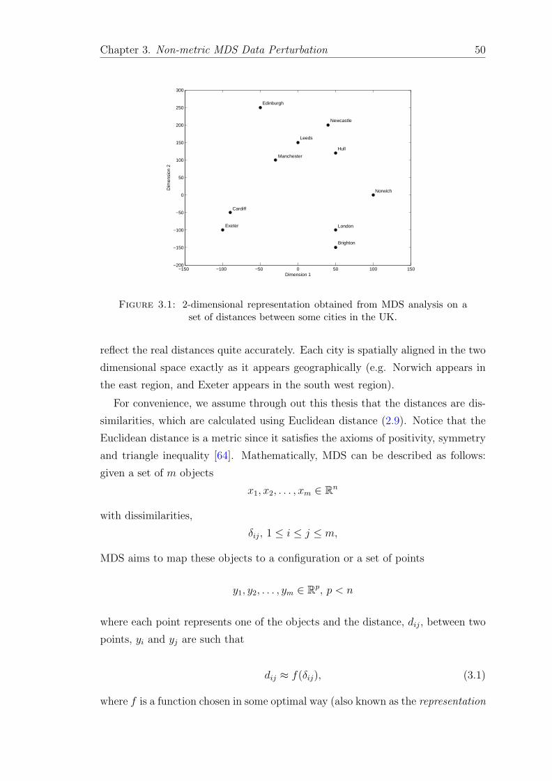
Chapter 3. Non-metric MDS Data Perturbation 50
−150 −100 −50 0 50 100 150−200
−150
−100
−50
0
50
100
150
200
250
300
Dimension 1
Dim
ensi
on 2
Edinburgh
Newcastle
Leeds
Manchester
Hull
Norwich
London
Brighton
Exeter
Cardiff
Figure 3.1: 2-dimensional representation obtained from MDS analysis on aset of distances between some cities in the UK.
reflect the real distances quite accurately. Each city is spatially aligned in the two
dimensional space exactly as it appears geographically (e.g. Norwich appears in
the east region, and Exeter appears in the south west region).
For convenience, we assume through out this thesis that the distances are dis-
similarities, which are calculated using Euclidean distance (2.9). Notice that the
Euclidean distance is a metric since it satisfies the axioms of positivity, symmetry
and triangle inequality [64]. Mathematically, MDS can be described as follows:
given a set of m objects
x1, x2, . . . , xm ∈ Rn
with dissimilarities,
δij, 1 ≤ i ≤ j ≤ m,
MDS aims to map these objects to a configuration or a set of points
y1, y2, . . . , ym ∈ Rp, p < n
where each point represents one of the objects and the distance, dij, between two
points, yi and yj are such that
dij ≈ f(δij), (3.1)
where f is a function chosen in some optimal way (also known as the representation

Chapter 3. Non-metric MDS Data Perturbation 51
function) that relates the dissimilarities in the original space to distances in the
new configuration and “≈” means equal with some small discrepancy.
In metric MDS, f is a specific continuous function that can be constructed in
several ways [18]. However, in non-metric MDS, f is a non-decreasing monotonic
function that maintains a monotone relationship between the dissimilarities and
the distances in the configuration. Monotonicity is a very important property,
which will be discussed further in Section 3.3, as it is central to the non-metric
MDS approach.
In MDS, a perfect transformation is usually not possible. Rather, what is
obtained is an approximation as a set of points whose distances approximate δij
as closely as possible. The requirement “as closely as possible” is quantified by
what is called a badness-of-fit measure or loss function, e2 =∑m
i,j (f(δij) − dij)2,
over all point configurations y1, y2, . . . , ym. Thus, with the lowest possible value of
e2, the best MDS is achieved.
Let ∆(2) = [δ2ij] be the matrix of squared dissimilarities, where δ2
ij = (xi −xj)(xi − xj)
T , and I be the m × m identity matrix. Define A = [−12δ2ij] and
B = HAH, where H is the centring matrix, H = I − n−11m1Tm, with 1n a vector
of ones. The matrix B is called inner product or Gram matrix, which can also be
represented by B = HXXTH. The minimum error solution is obtained from the
spectral decomposition of the Gram matrix. That is, to find the MDS configuration
from B, we can decompose B into
B = V ΛV T , (3.2)
where Λ is the diagonal matrix of the eigenvalues of B and V is the matrix of
corresponding eigenvectors. Since B is positive semi-definite and of rank p, it has
p non-negative eigenvalues and m− p zero eigenvalues. Hence, we can rewrite the
above equation (3.2) as
B = (VpΛ1/2)(VpΛ
1/2)T , (3.3)
where Vp is an m×p matrix containing the eigenvectors corresponding to non-zero
eigenvalues of B and Λ is an p × p diagonal matrix containing the eigenvalues.
The MDS solution is then given by

Chapter 3. Non-metric MDS Data Perturbation 52
Y = VpΛ1/2, (3.4)
where Y is an m× p coordinate matrix containing the points configuration in Rp.
This solution is known as classical MDS which is identical to PCA because the
Gram matrix of classical MDS has the same rank and eigenvalues up to a constant
factor as the covariance matrix of PCA [141]. Furthermore, both classical MDS and
PCA can lead to equivalent results and give precisely the same low-dimensional
representation [86]. To evaluate the goodness of the obtained configuration in
representing the input data, one can compute the proportion of variation explained
by p dimensions [40], i.e. ∑pi=1 λi∑
(positive eigenvalues)(3.5)
If the dissimilarities are treated directly as Euclidean distances, then it is pos-
sible to find a configuration of points in some lower space, that approximates the
distances in the original space, by decomposing the inner products of the input
data as described above. However, this would violate the privacy of the data as
the first few eigenvectors always maintain most of the data variances [120]. In
other words, such transformation embeds some information into the generated
configuration, which might be used to recover the original data. In this case, the
attacker can turn around the transformation to get the original data back, i.e. the
original data can be estimated as X = V Tp Y [80], and if the mean of the original
data is known to the attacker, s/he may obtain more accurate reconstruction by
adding on the mean, i.e. X = V Tp Y +µX . Note that if all the eigenvectors, V , are
included in the calculation, then the original data are exactly recovered [152].
Moreover, when the attacker knows a sample of the original data or the distri-
bution from where the original data have arisen, s/he may map the transformed
data with the original data through the computation of the eigen basis that spans
the known sample and the transformed data using the technique of PCA [108].
In other words, it would be possible to find a transformation basis that aligns the
principle components of the transformed data with the principle components of
the original data. This will be discuss in more details in Chapter 4. This mo-
tivates us to study and investigate non-metric MDS which seems to be able to
produce uncertain solution in terms of privacy preservation. In non-metric MDS,
the transformation is not based on eigenanalysis and thus no assumptions are made

Chapter 3. Non-metric MDS Data Perturbation 53
regarding the underlying structure of the data, whether “Gaussian” or otherwise.
Moreover, the features extracted by non-metric MDS in the lower-dimensional
space have no order of importance in terms of variance explanation but rather
define an arbitrary Cartesian coordinate system. Non-metric MDS uses the rank
order of distances not their actual values and derives the solution using an un-
known function. It causes data distortion which may hinder the attacker from
estimating the original data. However, non-metric MDS is able to retain most of
the properties used in distance-based data analysis so that accurate results can be
obtained from the perturbed data.
From a data utility point of view, classical MDS may destroy the local distri-
bution of the neighbourhood around data points. It often retains large distances
between data points and leads to the lost of the important underling structures
of the data [136]. Therefore, it may lead to poor results when distance-based
algorithms run on the perturbed data.
3.3 Non-Metric MDS Data Perturbation
In the context of PPDM, non-metric MDS can be used to disguise the original
data values and provide distorted data values (synthetic data) that preserve as
much as possible data properties for data mining task. That is, data privacy and
data utility are both preserved. Several methods have been recently proposed
for non-linear transformation, similar in spirit to non-metric MDS or even better.
Generally, these methods rely on the nearest neighbours graph theory where each
data point is connected to its k nearest neighbours as defined by a distance metric
and the weight of an edge in the graph is equal to the distance between its two
endpoints. Then, the nearest neighbours graph is used to construct a distance
matrix, which is then normalised and decomposed using the classical MDS to
extract the top eigenvectors and obtain the low-dimensional data. The isometric
feature mapping (ISOMAP) [161], the local linear embedding (LLE) [137] and
local MDS (LMDS) [29] are a few examples. Although these methods are able
to produce lower dimensional data that faithfully represents the original data,
they typically retain some geometric information which would be used to disclose
the privacy. Hence, we choose to use non-metric MDS as a perturbation tool in
order to increase the uncertainty about data in the lower dimensional space and
to effectively hide any information that would be embedded in the perturbed data
and used by the attacker to breach the privacy.

Chapter 3. Non-metric MDS Data Perturbation 54
Non-metric MDS attempts to find a configuration of points in some lower space
whose pairwise Euclidean distances have approximately the same rank order as
the corresponding dissimilarities in the higher space. This would make it harder
(if not impossible) to disclose the real values of the original data variables. The
final configuration resulting from this transformation is called perturbed data. Let
X be an m × n matrix representing the original data in the higher space, Rn, Y
be an m × p matrix represents the perturbed data in the lower space, Rp, and
∆ = [δij] be the dissimilarity matrix of X for i, j = {1, . . . ,m}. As described
earlier in Section 2.3.3, the Euclidean distance (L2 norm) is a measure that is used
most often to describe the dissimilarity between two data points, xi and xj
||xi − xj|| = δij =
√√√√ n∑k=1
(xik − xjk)2, (3.6)
where n is the number of dimensions, and xik and xjk are the kth attributes of
objects xi and xj, respectively.
The perturbation model is define by some transformation T
Y = T (X), (3.7)
where T : Rn → Rp is a non-metric MDS transformation such that
1. T preserves the rank ordering of the distances between objects in X and Y ,
i.e.
||xi − xj|| < ||xk − xl|| ⇐⇒ ||T (xi)− T (xj)|| < ||T (xk)− T (xl)||, (3.8)
and
2. T minimises the sum of squared differences of the distances, i.e. it minimises
∑i,j
(||xi − xj|| − ||T (xi)− T (xj)||)2. (3.9)
For presentation convenience, we use different notations to distinguish between
the distances in the original space, X, and the perturbed space, Y . The distances
between points in Y are ||T (xi)−T (xj)|| = dij. The above first condition is satisfied
through a monotonic function, f , that maintains a monotone relationship between
the dissimilarities, δij, and the distances, dij, in the lower space, Rp. The estimates

Chapter 3. Non-metric MDS Data Perturbation 55
of point locations in the lower dimensional space should yield predicted distances,
dij, between the points that “closely approximate” the observed dissimilarities,
δij, i.e. dij ≈ f(δij). To quantify the discrepancy (the stress) and to find the best
solution, the second condition should be applied.
The monotone relationship is obtained by a non-linear approach (monotonic
regression) that fits a non-linear function, f : δij 7→ dij, and minimises the stress,
S. The simplest way to evaluate the faithfulness of the transformation and to
quantify the stress is given by the squared error of representation, i.e.
e2 = (dij − dij)2, (3.10)
where dij are numbers representing a monotone least-square regression of dij on
δij (also known as disparities). That is, the disparities are merely an admissible
transformation of dij, chosen in optimal way, to minimise S over the data configu-
ration matrix, Y . The summation of e2 over all pairs (i, j) yields information loss
or raw stress,
S∗ =∑i,j
(dij − dij)2. (3.11)
To avoid the scale dependency, Kruscal [98] suggests a normalised version of
the raw stress, which is defined by
S =
√√√√∑i,j (dij − dij)2∑i,j d
2ij
. (3.12)
Non-metric MDS is quite similar to non-parametric procedures that are based
on ranked data. The dissimilarities, δij, are ranked by ordering them from lowest
to highest and the disparities, dij, should also follow the same monotonic ordering.
This constraint implies the so-called monotonicity requirement,
if δij < δkl then dij ≤ dkl. (3.13)
Note that ranks can be deduced from distances but distances cannot be de-
duced from ranks and thus a higher privacy is preserved. The non-metric solution
will provide the attacker with no information about the real distances between
data objects since any magnitude information is swept away by the monotonic
transformation. Note also that the rank orderings can be easily calculated from
the perturbed data. However, the questions that would likely be asked are “can

Chapter 3. Non-metric MDS Data Perturbation 56
Figure 3.2: An example shows the effect of the non-metric MDS perturbationon the geometry of “Nefertiti” face at different dimensions. The top left is theoriginal face. The following faces are the perturbed faces at n−5, n−10, n−20,
n− 30, n− 40, n− 50 and n− 60 dimensions, respectively.
the attacker learn anything from the ranks?”; and if s/he succeeded to learn some
information, “what is the probability that s/he infers or discloses the original
values?”. These questions will be answered in Chapter 4.
To see how much distortion the data Y have, consider “Nefertiti” image example
plotted in Figure 3.2. The image is represented by 3-dimensional mesh, which is
composed of an 3×n1 vertex matrix containing the position in 3-dimensional space,
and a face matrix of dimension 3× n2 containing the indexes of each triangulated
face. That is, the face matrix stores the topology (connectivity) of the mesh, while
the vertex matrix stores the geometry (position of the points). As we are interested
in the modification of the geometry only, we transformed the vertex matrix into
7 lower dimensions spaces (n1 − 5, n1 − 10, n1 − 20, n1 − 30, n1 − 40, n1 − 50
and n1 − 60,) and plotted the transformed faces. To easily observe the effect of
the perturbation, we use the classical MDS because the non-metric MDS heavily
flattens the shape even at high dimensions. The results provide insight into the
robustness of the perturbation in hiding the details of the face particularly at the

Chapter 3. Non-metric MDS Data Perturbation 57
Table 3.2: Iris dataset: data values of the first 10 rows in 4-dimensional space(original data X) and 3-dimensional space (perturbed data Y ).
X =
5.10 3.50 1.40 0.204.90 3 1.40 0.204.70 3.20 1.30 0.204.60 3.10 1.50 0.20
5 3.60 1.40 0.205.40 3.90 1.70 0.404.60 3.40 1.40 0.30
5 3.40 1.50 0.204.40 2.90 1.40 0.204.90 3.10 1.50 0.10
Y =
-2.25 0.47 -0.12-2.08 -0.67 -0.23-2.36 -0.34 0.04-2.30 -0.59 0.09-2.38 0.64 0.01-2.07 1.48 0.03-2.44 0.05 0.33-2.23 0.22 -0.09-2.33 -1.19 0.14-2.18 -0.47 -0.25
Table 3.3: Basic statistics of Iris dataset before and after the perturbation.
DataX Y
Dim 1 Dim 2 Dim 3 Dim 4 Dim 1 Dim 2 Dim 3
Mean 5.84 3.08 3.76 1.20 -0.85 -0.09 0.06
Std. Dev 0.83 0.44 1.77 0.76 1.71 0.96 0.38
Min 4.30 2 1.0 0.10 -2.77 -2.65 -0.86
Max 7.90 4.40 6.90 2.50 3.30 2.68 1.02
very low dimensions. For instance, it is hard to recognise the original face from
the perturbed face at n−50 or lower dimensions. Furthermore, the very low value
of average stress (1.24 × 10⁻¹⁸), especially for the perturbed face at the top row,
indicates the high utility of data in terms of distance preservation.
Another simple example is presented in Table 3.2. Here, we transformed the
well-known Iris dataset, which is represented by a 4-dimensional data matrix, X,
and generated the perturbed data, Y , in 3-dimensional space. The Iris dataset
consists of 150 instances and 4 continuous attributes measured from three different
iris plant species. One class (Setosa) is linearly separable from the other two classes
(Versicolour and Virginica). The latter are not linearly separable from each other.
The data values of both data matrices X and Y substantially look different from
each other and comparable. The basic statistics for all attributes of the entire
dataset are shown in Table 3.3.
One distinguishing feature of Non-metric MDS is that it can produce uncorre-
lated features in the lower dimensional space [40]. The uncorrelated features may
provide further privacy, particularly against attacks that attempt, under certain
circumstances, to exploit the correlation between features in order to disclose the
original data [65, 80, 88, 120]. Figure 3.3 shows a visual representation of the

Chapter 3. Non-metric MDS Data Perturbation 58
0 1 2Petal width
2 4 6Petal length
2 3 4Sepal width
6 80
1
2
Sepal length
Peta
l wid
th
2
4
6
Peta
l length
2
3
4
Sepal w
idth
5
6
7
8
Sepal l
ength Setosa
VersicolourVirginica
(a) X
−0.5 0 0.5 1Dim 3
−2 0 2Dim 2
−2 0 2
−0.5
0
0.5
1
Dim 1
Dim
3
−2−1
012
Dim
2
−2
0
2
Dim
1
SetosaVersicolourVirginica
(b) Y
Figure 3.3: Correlations among pairs of variables in: (a) the original data, X,and (b) the perturbed data, Y . Histograms of the variables appear along the
matrix diagonal; scatter plots of variable pairs appear off-diagonal.
correlations among the pairs of variables in both data X and Y as well as the data
distribution of each variable. The new variables of non-metric MDS solution seem
uncorrelated and have different distributions from the original ones so that they
may better describe the variability of the data. It is difficult to draw any single
regression line that can predict the second dimension from the first, and vice versa.
However, the dispersion of groups remains unchanged, i.e. groups are reasonably
separable. This is an important property in distance-based learning. Table 3.4
shows the correlation coefficients of the variables. The correlation coefficients of
variables in the perturbed were very small and insignificant.
Table 3.4: Correlations between variables in (a) the original data, X, and (a)the perturbed data, Y .
(a)
Dim 1 Dim 2 Dim 3 Dim 4Dim 1 1.00Dim 2 -0.12 1.00Dim 3 0.87 -0.43 1.00Dim 4 0.82 -0.37 0.96 1.00
(b)
Dim 1 Dim 2 Dim 3Dim 1 1.00Dim 2 0.00 1.00Dim 3 0.00 -0.00 1.00
To gain insight into the superiority of non-metric MDS in preserving the pair-
wise distances, we plot the distribution of the dissimilarities at three lower dimen-
sions, i.e. p = 1, p = 2 and p = 3, and compare it with the original dissimilarities.
The results are shown in Figure 3.4. The distribution remains unchanged and

Chapter 3. Non-metric MDS Data Perturbation 59
−4 −2 0 2 4 6 80
50
100
150
200
250
300X
Distance−4 −2 0 2 4 6 80
50
100
150
200
250
300p=3
Distance
−4 −2 0 2 4 6 80
50
100
150
200
250
300p=2
Distance−4 −2 0 2 4 6 80
50
100
150
200
250
300
350
400p=1
Distance
Figure 3.4: Distribution of dissimilarities at the original data (top left), at3-dimensions (top right), at 2-dimensions (bottom left) and at 1-dimension (bot-
tom right).
almost identical indicating that non-metric MDS can properly represent the dis-
similarities at high dimensional spaces, i.e. p = 3 and p = 2. For the data in
1-dimensional space, the distribution is slightly changed where small dissimilari-
ties are increased. The deviation in distance between X and Y at 3-dimensional
space is very low (0.21 × 10⁻¹⁶), indicating a good data utility for the task of
distance-based mining. This implies that non-metric MDS is able to preserve the
underlying distance-related properties quite accurately. If the distance is well pre-
served, one would expect that for any two objects xi and xj that appear in the
same cluster in X, their mappings yi and yj will also appear together in the same
cluster in Y . Moreover, non-metric MDS is capable of eliminating irrelevant, re-
dundant, and noisy features and thus it can facilitate the distance-based learning
process and produce more accurate results [159].
Non-metric starts from a dissimilarity matrix so that it can be used for data
that do not originally have a vector space representation. Since non-metric MDS

Chapter 3. Non-metric MDS Data Perturbation 60
operates on dissimilarities, the data type of the underlying variables is unimpor-
tant and thus one has not to worry about the type of the data attributes to be
either quantitative or qualitative. However, to make it possible to obtain an objec-
tive or scale-invariant result, some normalisation must be performed prior to the
computation of dissimilarities for both quantitative and qualitative variables. In
addition, non-metric MDS perturbs all attributes together under one single trans-
formation and thus instead of assessing the quality of privacy for each attribute
independently it would be easier to use a single unified metric.
3.3.1 Monotonicity Preservation
Given a set {δij : i < j} of the M elements of the upper triangle of the dissimi-
larity matrix, ∆, let M = m(m−1)/2 be the number of all possible dissimilarities,
δij, that can be calculated from the data matrix, X, sorted in ascending order to
obtain the ordered sequence:
δ1ij ≤ δ2
ij ≤ . . . ≤ δMij . (3.14)
Ideally, we would like the distances, dij, in Y to be in ascending order too
d1ij ≤ d2
ij ≤ . . . ≤ dMij . (3.15)
The problem is to find the estimated value, dij, for each dij such that the stress,
S, is minimised subject to the monotone requirement that
d1ij ≤ d2
ij ≤ . . . ≤ dMij . (3.16)
To solve this monotonic regression problem, Kruskal [98] proposed a Pooled-
Adjacent-Violator (PAV) algorithm that starts with a set of M distances obtained
from an initial configuration and attempts to not violate the monotonicity require-
ment for any pair of adjacent values (dl−1ij , dlij) and (dlij, d
l+1ij ).
To illustrate the basic idea of PAV algorithm, consider the example in Table
3.5. Assume that we have ranked a set of dissimilarities, δij, between a set of
objects of data X (as in the second column). Assume also that we have then
obtained a set of distances, dij, (as in the third column) from the configuration,
Y . All dij can be represented in M blocks each containing a single distance,
b1, b2, . . . , bM . The block is a data structure used to store and manipulate one or

Chapter 3. Non-metric MDS Data Perturbation 61
Table 3.5: Derivation of disparities using PAV algorithm.
(i, j) rank(δij) dij d1ij d2
ij d3ij d4
ij
Finaldij
(1,2) 1 4 3.5 3 2.5 2.5 2.5—
(1,3) 2 3 3.5 3 2.5 2.5 2.5— —
(1,4) 3 2 2 3 2.5 2.5 2.5— — —
(2,3) 4 1 1 1 2.5 2.5 2.5— — — — —
(2,4) 5 5 5 5 5 4 4— — — —
(3,4) 6 3 3 3 3 4 4— — — — —
more values of distance; it enables us to compute the arithmetical mean of each
block’s members and also compare each block with its preceding and succeeding
block. Note that distances, dij, can be treated as initial disparities, dij. To
achieve the monotonicity requirement, each distance should preserve the right
order, i.e. diij ≤ di+1ij . That is, for each block bi, its member values must be
greater or equal to its preceding block’s, bi−1, member values, and meanwhile, less
or equal to its succeeding block’s, bi+1, member values. Beginning with the first
block corresponding to the smallest dissimilarity, d12, we check and find it has not
satisfied the requirement. We should modify d12 to become smaller or equal to
d13. To do so, we merge the two blocks in one block and take the arithmetical
mean of its members (d12 + d13)/2 = (4 + 3)/2 = 3.5 = d112 = d1
13. This yields the
distances in the fourth column of Table 3.5. However, the first trial solution (i.e.
d1ij) satisfies the monotonicity requirement only for its first two elements (i.e. first
block) and we must check other elements or blocks. Because d114 = 2 is smaller
than the preceding values, we create a new block by calculating the average of the
first three distances (3.5 + 3.5 + 2/3 = 3). This yields the distances in the fifth
column of Table 3.5. Again, we hope to satisfy the monotonicity requirement in
all remaining distances in this trial d2ij. However, this sequence still violates the
monotonicity since the values of the new block, that has just formed in the previous
trial, is greater than the succeeding block (d223 < 3). Therefore, we merge the two
blocks in one block and average its members. The sixth column of Table 3.5 shows
the new disparities of the third trial in three different blocks. We repeat the same

Chapter 3. Non-metric MDS Data Perturbation 62
procedures for all other distances until no block violates the monotonicity. The
last column of Table 3.5 shows the sequence of the final disparities, dij, obtained
by monotone regression for the first iteration. At this point, we can evaluate the
stress, S, to determine if it is the best achieved so far or not. That is, if no
improvement is possible, then accept Y as a final configuration. Otherwise, the
points of Y must be moved along the direction of the gradient. This gives new
distances, dij, which can be used to compute new disparities, dij, for the second
iteration, and so on. The steps of PAV algorithm are shown in algorithm 3.1.
Algorithm 3.1 PAV Algorithm
Input: D: a set of M distances, d1, d2, . . . , dM .Output: D: a set of M ordered disparities, d1 ≤ d2 ≤ . . . ≤ dM .{Assign each distance, di, to a single block, bi}for i = 1 to M − 1 do{Check if any pair of adjacent values (di, di+1) violates the monotonicity re-quirement}if di > di+1 then
Pool all members of block bi and bi+1; and replace all of them by theiraverageMerge bi and bi+1 into one block{Go backwards and check if di, di−1 obey the monotonicity requirement}if di < di−1 then
Pool all members of block bi and bi−1; and replace all of them by theiraverageMerge bi and bi−1 into one block
end ifend if
end for
3.3.2 Distance Preservation
After we predicted the disparities, dij, that preserve the same rank order of the
dissimilarities, δij, by using the PAV algorithm, a new configuration, Y , is sought
such that the disparities of distances, dij, obtained from Y and the estimated
distances, dij, are minimised. We use the stress, S, to measure such disparity.
The steepest descent method [98] is used to find the nearest local minimum
of the function S where the gradient of this function can be calculated at each
iteration. Let y0 = S(x0) be the initial point. Move downhill gradually along
the curve corresponding to the function S in the direction of the local downhill
gradient, −∇S(x0), which is usually calculated by taking the partial derivatives
of S.

Chapter 3. Non-metric MDS Data Perturbation 63
The non-metric MDS solution is usually found by choosing an initial configu-
ration in Rp, Y 0, and moving its points around, in iterative steps, to approximate
the best model relation, dij ≈ f(δij). In other words, the coordinates of each point
in Rp are adjusted in the direction that maximally reduces the stress. That is,
the start point would indeed affect the processing time required to find the best
solution. Decomposing the matrix ∆(2) into its eigenvalues and their associated
eigenvectors, which is equivalent to the classical metric MDS, is one possible way
to start with a quite good initial configuration. Typically, the pairwise distances
are quite faithfully retained at this configuration [40]. We assume that ∆(2) is
positive semi-definite and of rank p. Hence, it has p non-negative eigenvalues and
n−p zero eigenvalues. However, if ∆(2) has more than (n−p) negative eigenvalues,
then Y k can be padded with zeros to achieve p-dimensions.
Note that the classical metric MDS solution would lead, in some cases, to accept
the initial configuration as the best configuration obtained, i.e. Y 0 = Y , such that
the stress is at an optimal local minimum. This, indeed, compromises the privacy
because the dissimilarity matrix can be accurately derived from the perturbed
data using matrix algebra, as described above in Section 3.2. If the dissimilarity
matrix is estimated, then it can be used to disclose the original data [165]. In order
to avoid such a problem, we can use a random initial configuration to start with
and iteratively seek for the best fit where the stress is minimised. Alternatively,
we can replicate the running of non-metric MDS multiple times, each starts at a
different randomly chosen initial configuration. Then, the configuration with the
lowest value of stress is selected.
Let k be the iteration number and Y k be the configuration at iteration k. We
want to find the best data configuration such that the stress, S, is at a local mini-
mum. Let us now measure S by calculating both the distances, dij, obtained from
Y k and the corresponding disparities, dij, which are generated using the steps de-
scribed earlier in Section 3.3.1. To construct the next configuration, Y k+1, subject
to minimising S, we should compute the gradient. The partial derivatives of S
at each coordinate of configuration Y k form the gradient, which indeed expresses
the direction of steepest descent. Let yki and ykj be two points in configuration
Y k and we want to find a new position for point yk+1i in the configuration Y k+1
relative to point yk+1j in the direction where S is minimised. The gradient at the
configuration Y k is given by

Chapter 3. Non-metric MDS Data Perturbation 64
gkia = − ∂S
∂ykia= S
[(dij − dij∑M
i,j (dij − dij)2− dij∑M
i,j d2ij
)((ykia − ykja)
dij
)], (3.17)
where a is the coordinate number, a = {1, 2, . . . , p}. The new position at coordi-
nate a in the configuration Y k+1 is defined by
yk+1ia = ykia + αk gkia, (3.18)
where αk is a downhill step-size and gkia is the corresponding entry in the negative
gradient matrix, Gk, of stress S at configuration Y k. The overall improvement
relative to all remaining points in Y k+1 is
yk+1ia = ykia + αk
m−1∑j=1j 6=i
gkja, for all a = {1, 2, . . . , p}. (3.19)
That is, the new point yk+1i is improved relative to the point yk+1
j and moving Y k
along the direction of the negative gradient will tend to make Sk+1 to be smaller
than Sk. In other words, the stress function is expected to decrease towards a
local minimum. However, if the stress goes up at this iteration, then the process
is terminated and the configuration Y k is chosen to be the final configuration.
Figure 3.5 shows an example of how non-metric MDS could generate data that
statistically useful for distance-based analysis. In this example, we generated three
datasets each of which has 3 dimensions and has different distribution (Swiss roll,
Gaussian and 3-clusters). Then, we transformed them into 2-dimensional space
using non-metric MDS. The perturbed data exhibit a perfect preservation of both
the pairwise distances and the underlying data structure. The average stress for
all datasets was 1.94× 10⁻¹⁶.
3.3.3 How Many Dimensions to Retain?
An important issue in non-metric MDS mapping is the choice of the number of
dimensions in the lower-dimensional space. Typically, when the data are mapped
into a high number of dimensions, the mapping error is very small but that may
lead to an increasing in computation complexity. On the other hand, when the
data are mapped into too few dimensions, they might not reveal the underlying
data structure. The most obvious criterion for choosing the number of dimensions,

Chapter 3. Non-metric MDS Data Perturbation 65
Figure 3.5: Three different datasets with different geometrical shapes. Thetop row are the original data at 3-dimensional space. The bottom row are the
perturbed data at 2-dimensional space using non-metric MDS.
p, is to select a configuration, among a set of configurations at different p, that
gives the smallest value of stress, S. One possible way to find the appropriate
number of p is to plot S as a function of the dimensionality and then to look
for an elbow in the plot. The stress reflects how well the dissimilarities, δij, of
the original data, X, or their transformation, dij, are fitted by the corresponding
distances, dij, in the perturbed data, Y . Conveniently, it seems to be a suitable
measure of loss of utility of Y over X for distance-based analysis. The stress is
invariant under uniform stretching and shrinking of the configuration [98]. As the
stress is a residual sum of squares, it is positive, and the smaller the better. It
can be expressed as a percentage, with 0% stress being equivalent to a perfect
configuration, i.e. one that presents a perfect monotone relationship between
dissimilarities and distances.
Kruskal [97] suggests a rule of thumb to decide if the stress value is sufficiently
small or not. The rule is given in Table 3.6. As we will see in Chapter 5, we
experimentally observe that as p increases, S decreases. The data at the higher
dimensionality often maintain the best fit of the original data and introduce higher
utility for distance-based analysis.

Chapter 3. Non-metric MDS Data Perturbation 66
Table 3.6: Kruskal’s rule to decide on the quality of the lower-dimensionalspace.
Stress (S) Mapping Quality
S > 20% Poor5% < S ≤ 10% Fair2.5% < S ≤ 5% Good0 < S ≤ 2.5% Excellent
S = 0 Perfect
Table 3.7: Stress values at one reduced dimension using Minkowski distancewith different exponents.
DatasetMinkowski exponents (r)
r = 1 r = 2 r = 3 r = 4 r = 5
Wine 0.0492 0.0068 0.1154 0.2017 0.3245BCW 0.0428 0.0076 0.0826 0.1022 0.2663HRDigits 0.0080 0.0000 0.0144 0.0276 0.0374ImgSeg 0.0116 0.0000 0.0407 0.0523 0.0623
As a related topic of choosing the right dimension that minimises the stress,
one my also think in the used distance metric. As the quality of the perturbed
data for distance-based mining is basically based on the size of distance lost as
a result of the transformation, the relationship between a pair of objects should
accurately be reflected by a suitable distance function. This may facilitate the
task of data mining algorithm and enable better patterns discovery. To assess the
utility in terms of distance metrics, we calculate the Minkowski distance between
data objects in four datasets, taken from the UCI machine learning repository [58],
using different exponent, r, varied from 1 to 5. Then, for each dataset, we trans-
formed the data into one reduced dimension, i.e. n− 1. Table 3.7 shows the stress
values with different exponents. The results confirms that the Euclidean distance
represents the best metric to use to calculate the dissimilarities. However, it has
been shown in [43] that certain Minkowski distance matrices are exchangeable. In
other words, the solution found by non-metric MDS using Euclidean distance can
be exchanged by the solution using Manhattan distance or Max distance with-
out changing the stress. Although we use, throughout this thesis, the Euclidean
distance as a dissimilarity metric, further instigation is required to evaluate the
influence of proximity on the overall performance and decide whether any small
differences in the stress values are significant. This is left for future work.
Chapter 3. Non-metric MDS Data Perturbation 67
3.3.4 Non-Metric MDS Algorithm
The non-metric MDS algorithm is composed of three main phases as follows:
1. Initial phase: Calculate the dissimilarities, δij, of any pair of objects in the
original data. Then, construct an initial configuration, Y 0, in the required
lower dimensional space, say p, either randomly or using the classical MDS.
2. Non-metric phase: Use the PAV algorithm to derive any estimated dis-
tance, dij, from the current configuration, Y t, such that the monotonicity is
completely satisfied.
3. Metric phase: Move the current configuration, Y t, towards a better loca-
tion using the step function, defined in (3.19), to obtain a new configuration,
Y t+1, such that the stress, S, is minimised to a very small value.
That is, the algorithm starts from the initial phase. Then, it iteratively opti-
mises the non-metric phase. Finally, it evaluates the best fit in the metric phase
until the rank order of all dissimilarities is satisfied. More precisely, the non-metric
MDS algorithm requires the following steps:
1. Choose the dimension, p, and determine an initial configuration, Y .
2. Calculate the resulting distances, dij, between each pair of points in Y .
3. Estimate the new set of disparities, dij, by using a monotone regression that
relates dij to δij.
4. Evaluate the best-fit of dij and dij and calculate the stress, S.
5. Improve Y a little by moving it around in the direction that minimises S
using the steepest descent.
6. Repeat Steps 2 to 5 until no improvement is possible.
Non-metric MDS uses a monotonic regression to map the dissimilarity and thus
it is very computational expensive. In this work, we did not make any particular
effort to reduce the complexity as the major concern is to generate perturbed
data that are useful for distance-based data mining whilst the privacy is well
protected. However, alternative approach to overcome the computational burden is
to use monotone splines [133] which provide flexibly shaped but smooth monotonic
transformations [181].
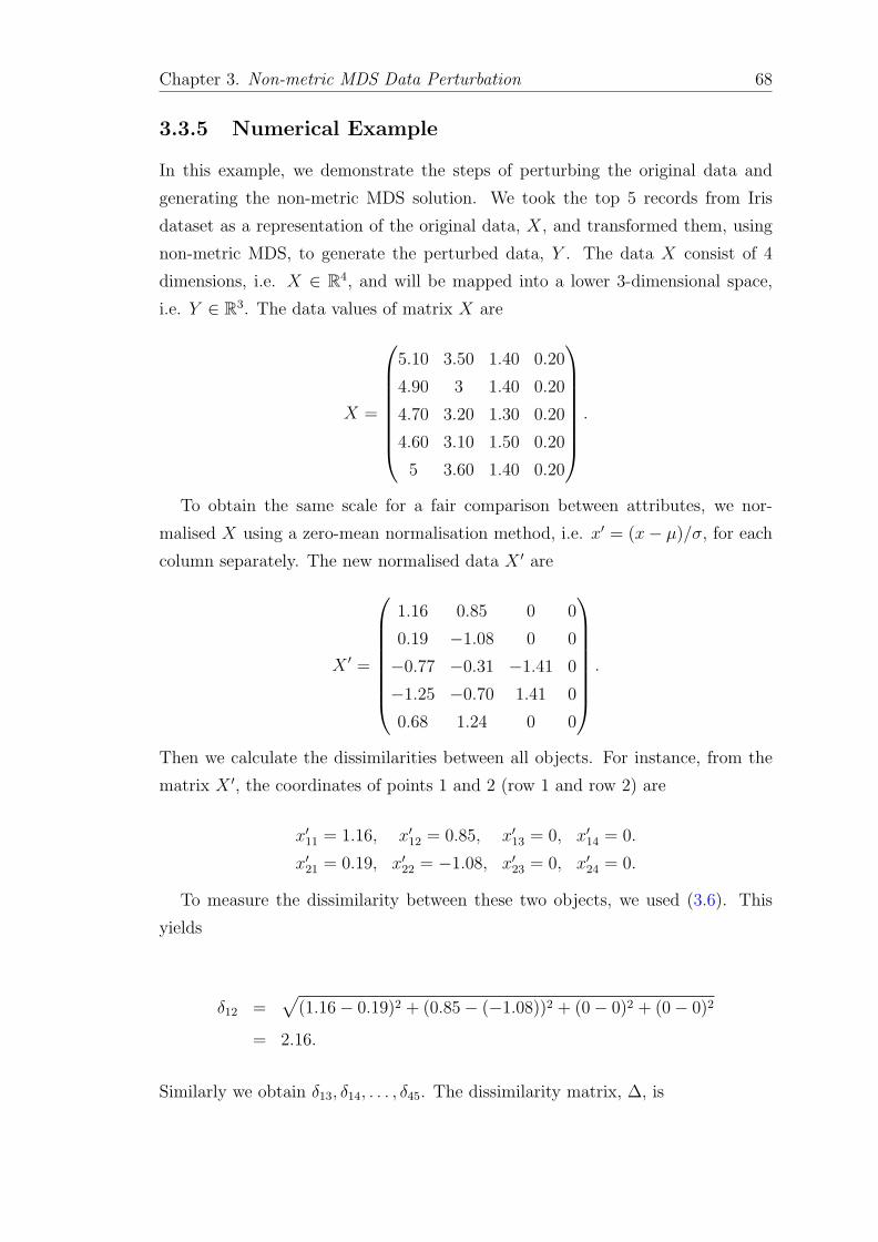
Chapter 3. Non-metric MDS Data Perturbation 68
3.3.5 Numerical Example
In this example, we demonstrate the steps of perturbing the original data and
generating the non-metric MDS solution. We took the top 5 records from Iris
dataset as a representation of the original data, X, and transformed them, using
non-metric MDS, to generate the perturbed data, Y . The data X consist of 4
dimensions, i.e. X ∈ R4, and will be mapped into a lower 3-dimensional space,
i.e. Y ∈ R3. The data values of matrix X are
X =
5.10 3.50 1.40 0.20
4.90 3 1.40 0.20
4.70 3.20 1.30 0.20
4.60 3.10 1.50 0.20
5 3.60 1.40 0.20
.
To obtain the same scale for a fair comparison between attributes, we nor-
malised X using a zero-mean normalisation method, i.e. x′ = (x− µ)/σ, for each
column separately. The new normalised data X ′ are
X ′ =
1.16 0.85 0 0
0.19 −1.08 0 0
−0.77 −0.31 −1.41 0
−1.25 −0.70 1.41 0
0.68 1.24 0 0
.
Then we calculate the dissimilarities between all objects. For instance, from the
matrix X ′, the coordinates of points 1 and 2 (row 1 and row 2) are
x′11 = 1.16, x′12 = 0.85, x′13 = 0, x′14 = 0.
x′21 = 0.19, x′22 = −1.08, x′23 = 0, x′24 = 0.
To measure the dissimilarity between these two objects, we used (3.6). This
yields
δ12 =√
(1.16− 0.19)2 + (0.85− (−1.08))2 + (0− 0)2 + (0− 0)2
= 2.16.
Similarly we obtain δ13, δ14, . . . , δ45. The dissimilarity matrix, ∆, is

Chapter 3. Non-metric MDS Data Perturbation 69
−1.5−1
−0.50
0.51
−2
−1
0
1
2−2
−1.5
−1
−0.5
0
0.5
1
3
5
2
4
1
(a) Initial configuration
0.2 0.4 0.6 0.8 1 1.2 1.4 1.6
1.4
1.6
1.8
2
2.2
2.4
2.6
2.8
3
3.2
Dissimilarities
Dis
tance
s/D
isparitie
s
DistancesDisparities
(b) Shepard plot
Figure 3.6: (a) The initial configuration in 3-dimensional space. (b) Shepardplot shows how the distances approximate the disparities (the scatter of bluecircles around the red line), and how the disparities reflect the rank order of the
dissimilarities (the red line is non-linear but increasing).
∆ =
0 2.16 2.66 3.19 0.62
2.16 0 1.87 2.05 2.37
2.66 1.87 0 2.89 2.55
3.19 2.05 2.89 0 3.08
0.62 2.37 2.55 3.08 0
.
Since the data samples are very small and to avoid getting trapped in a local
minimum of the function S too soon, we start from a random initial configuration.
The initial configuration data matrix, Y 0, is
Y 0 =
−1.08 0.28 0.89
−0.65 −1.38 0.36
0.75 0.10 −0.21
0.52 1.42 0.45
0.45 −0.42 −1.49
,
and it is plotted in Figure 3.6(a).
To show the degree to which the distances, dij, between points in Y 0 agree with
the dissimilarities, δij, we plot the distances against the dissimilarities as shown
in Figure 3.6(b). It is clear from the figure that the regression line is not fitted
well which means that the disparities, dij, are still not in same rank order as the

Chapter 3. Non-metric MDS Data Perturbation 70
Table 3.8: Predicted disparities, dij , using PAV algorithm.
(i, j) dij d1ij d2
ij d3ij
(1,2) 3.13 3.13 3.13 2.88— — —
(1,3) 3.54 3.48 2.80 2.88—
(1,4) 3.41 3.48 2.80 2.88— —
(1,5) 1.43 1.43 2.80 2.88— — — —
dissimilarities and more iterations should be taken until a better solution is found.
Assume that a configuration Y at iteration t has been generated such that:
Y t =
−2 0.11 −0.50
0.54 −1 0.95
1.30 −1.08 0
0.62 1.86 0.81
−0.86 0.16 −1.36
.
To compute the coordinates for the first point, y1, in the new configuration, Y t+1,
we should calculate the gradient such that the stress, S, is minimised. From Y t,
we calculate the distances between point y1 and other points y2, y3, y4 and y5. The
distances are
d12 = 3.13, d13 = 3.54, d14 = 3.41 and d15 = 1.43.
Using PAV algorithm as described in Section 3.3.1, the predicted disparities are
d12 = 2.88, d13 = 2.88, d14 = 2.88 and d15 = 2.88.
Table 3.8 shows the procedures that have been taken to find dij. Let∑10
i<j (dij −dij)
2 = 0.03 be the sum of the squared difference between all the distances and
the disparities and∑10
i<j d2ij = 75.73 be the sum of all the distances.
Applying (3.19) yields (for α = 0.2 and S = 0.01 from the previous iteration,
t− 1)

Chapter 3. Non-metric MDS Data Perturbation 71
yt+111 = −2 + 0.2× 0.01
[4∑j=1j 6=1
(d1j − d1j∑M
1<j (dij − dij)2− d1j∑M
1<j d21j
)((−2− yj1)
d1j
)]
= −2 + 0.002
[(3.13− 2.88
0.03− 3.13
75.73
)((−2− 0.54)
3.13
)+(
3.54− 2.88
0.03− 3.54
75.73
)((−2− 1.30)
3.54
)+(
3.41− 2.88
0.03− 3.41
75.73
)((−2− 0.62)
3.41
)+(
1.43− 2.88
0.03− 1.43
75.73
)((−2− (−0.86))
1.43
)]
= −2 + 0.002
[− 6.73 + (−20.41) + (−13.57) + 38.68
]= −2− 0.01
= −2.01.
Similarly, we obtain yt+112 = 0.21 and yt+1
13 = −0.59. That is, the coordinates of
point yt+11 are (-2.01,0.21,-0.59). The same procedures will be performed for all
other points (yt+12 , yt+1
3 , yt+14 and yt+1
5 ). The configuration, Y t+1, is as follows:
Y k+1 =
−2.01 0.21 −0.59
0.55 −1.02 0.95
1.29 −1.11 0.10
0.63 1.87 0.83
−0.87 0.16 −1.36
.
Finally, after a number of iterations until a local minimum is reached, the data
values of the final solution are
Y =
1.36 0.39 −0.26
−0.60 −0.21 −0.90
−0.34 −1.56 0.38
−1.72 0.98 0.35
1.30 0.39 0.39
,

Chapter 3. Non-metric MDS Data Perturbation 72
0 10 20 30 40 500
0.02
0.04
0.06
0.08
0.1
0.12
0.14
0.16
0.18
0.2
#iterations (t)
Str
ess
(S)
Figure 3.7: The stress, S, at different iterations.
−2−1
01
2
−1
0
1
2
3−1
−0.5
0
0.5
1
3
24
5
1
(a) Final configuration
0.2 0.4 0.6 0.8 1 1.2 1.4 1.60.5
1
1.5
2
2.5
3
3.5
Dissimilarities
Dis
tance
s/D
isparitie
s
DistancesDisparities
(b) Shepard plot
Figure 3.8: (a) The final configuration in 3-dimensional space. (b) Shepardplot shows a perfect fit where the disparities are exactly coincided with the
distances.
and the stress, S, equals 8.12 × 10⁻⁷. Figure 3.7 shows the function of S at
each iteration. The final solution, Y , is graphically shown in Figure 3.8(a). The
Shepard plot of both the distances, dij, and the predicted distances, dij, at the final
iteration is depicted in Figure 3.8(b). All points in the plot lie on the regression
line indicating that the dissimilarities, δij, are perfectly related to the distances,
dij, and hence, the underlying structure of the original data, X, remains preserved.
Once the final configuration Y is generated, we can use it to carry out the
distance-based analysis. The data Y are totally different from data X and the

Chapter 3. Non-metric MDS Data Perturbation 73
columns of both X and Y are irrelevant, have different pdfs and with different
ranges. However, data Y are analytically as useful as data X, because the pairwise
distances are still largely preserved.
3.4 Geometry of Non-Metric MDS
To guarantee the successfulness of the non-metric MDS technique in preventing
the disclosure, the information embedded in the new space after transformation
should be downgraded as much as possible. Non-metric MDS can effectively em-
bed a set of objects into a Euclidean space that preserves the rank order of the
pairwise distances between all objects as closely as possible. However, it manages
to contain uncertainty about the original data and hinder the attacker from ex-
actly determine the locations of points in the higher dimensional space. A high
degree of uncertainty in the data can lead to the best privacy-preserving solution.
In non-metric MDS, the perturbed data, Y , is subject to high uncertainty since
the monotone regression geometrically implies that Y are moved iteratively in the
direction that minimises the stress, S, and therefore, the points are placed within
an uncertain area under the restriction of monotonicity. To illustrate the idea of
placing points in non-metric MDS solution, consider the following example. Let
x1, x2, . . . , xM denote the set of unknown disparities, dij, and a1, a2, . . . , aM denote
the set of known distances in the space Y . Assume that all dij are monotonically
ordered as
0 ≤ x1 ≤ x2 ≤ . . . ≤ xM .
and the monotone regression problem is to minimise the raw stress, S∗, which is
defined by
S∗ =M∑i=1
(xi − ai)2.
Consider the case of only the first two inequalities 0 ≤ x1 ≤ x2. The shaded
area above the curve in Figure 3.9(a) shows the area in which these two inequalities
are held. Let us pick up any point in the shaded area (e.g. a1 = 1 and a2 = 2).
That is, choosing values x1 = 1 and x2 = 2 gives S∗ without violating the order
restriction. If ai is outside the shaded area, then xi must be somewhere on the
border of the shaded area and close to ai as much as possible. Similarly, if we
consider one more inequality, i.e. 0 ≤ x1 ≤ x2 ≤ x3, the graphical representation

Chapter 3. Non-metric MDS Data Perturbation 74
(a) 0 ≤ x1 ≤ x2 (b) 0 ≤ x1 ≤ x2 ≤ x3
Figure 3.9: Points arrangement for which the inequalities order is not violated.
will be now in 3-dimensions as shown in Figure 3.9(b). The area in which the
three inequalities hold is represented by a cone. The monotone regression would
project a1, a2 and a3 onto this cone and choose x1, x2 and x3 that are very close
to a1, a2 and a3.
From the above example, we conclude that the monotone regression finds a vec-
tor of dij that is in the same order of δij and as close as possible to the vector of
dij. Geographically, the non-metric MDS solution relaxes the points’ arrangement
in the lower space so that it increases the uncertainty of the exact points’ loca-
tions. Note that the large number of ordinal distances the more restricted areas to
place points in the lower dimensional space. For instance, placing a point without
violating three distance inequalities would give a less restricted area than placing
it when there are ten inequalities. As we will see later in the distance-based attack
in Chapter 4, the attacker will utilise only the sequence of distances between the
attacked point and the other n + 1 known points in order to attack any point in
the lower dimensional space. However, if the data objects are mapped using the
rank order of their corresponding distances not their magnitudes, then the task
would be complicate and thus the risk of the disclosure is minimised.

Chapter 3. Non-metric MDS Data Perturbation 75
3.5 On the Proximity for Non-Metric MDS
As described earlier in Section 3.2, metric MDS attempts to find a low-dimensional
configuration of points that best represents objects such that the distance between
any two points matches their dissimilarities as closely as possible. On the other
hand, non-metric MDS considers only the rank ordering of the dissimilarities as
meaningful. The magnitude of the dissimilarities, δij, are replaced by a higher
abstraction level describing the relationship between data objects, i.e. δij < δkl.
For instance, if δij = 2 and δkl = 3, an ordinal model reads this only as δij < δkl
and constructs the distances, dij and dkl, in the lower dimensional space so that
dij < dkl. Notice that any ordering of m(m−1)/2 distances between m data points
can be realised in a Euclidean space of m− 1 dimensions [149].
When using non-metric MDS, it becomes irrelevant which proximity measure is
used, because any proximity measure, in general, yields equivalent rank ordering
and can be embedded into low-dimensional space [1, 12]. Furthermore, arbitrary
distance functions can accurately be mapped to an Euclidean distance domain
which would also simplify the computation of distances [175]. To illustrated the
idea behind this, let X1 and X2 be two variables in data X and assume that they
are both standardised so that their means are zero and their sum of squares is
equal to 1. The Euclidean distance between X1 and X2 is given by
d(Xi, Xj) =
(m∑l=1
(xil − xjl)2
)1/2
=
(m∑l=1
x2il +
m∑l=1
x2jl − 2
m∑l=1
xilxjl
)1/2
.
(3.20)
Since Xi and Xj are standardised, the sumsm∑l=1
x2il and
m∑l=1
x2jl are both equal to
1 and thus
d(Xi, Xj) =
(2− 2
m∑l=1
xilxjl
)1/2
. (3.21)
This leaves us with the non-constant term,m∑l=1
xilxjl, which is exactly equivalent
to the correlation coefficient, i.e.

Chapter 3. Non-metric MDS Data Perturbation 76
corr(Xi, Xj) =m∑l=1
xilxjl. (3.22)
On the basis of the above result, we can express the Euclidean distance measure
relative to any another proximity measure while the ordinal characteristics remain
unchanged. Similarly, one can show that other distance measures that are typically
highly correlated with the Euclidean distance (e.g. Manhattan and Max distances)
are also monotonically closely related to the correlation coefficient. The non-metric
MDS can use the inter-correlation matrix, which is then converted to a matrix in
which the correlation coefficients are replaced with the rank order values, i.e. the
highest correlation value receives a rank order of 1, the next highest receives a
rank order of 2 and so on. It then attempts to arrange these sequences so that
the more closely related objects are mapped closer together than the less closely
related objects.
As the optimal fit of data in the low-dimensional space is often obtained when
the stress is minimal, much care should be taken when deriving proximities among
data objects. In general, if the average distance is fairly well preserved in the
perturbed data, then any distance-based data mining algorithm can accurately
identify patterns within the data and often gives quite similar results as on the
original data. However, when the analysis requires a strict judgement on the
similarity between objects (e.g. as in the case of psychological data analysis [163]),
it would be appropriate to define a measure that is invariant to the transformation
and induce the same rank order when comparing objects.
3.6 Summary
In this chapter, we present our data perturbation technique using non-metric MDS
and show how it is possible to generate data that preserve much properties for
distance-based data mining while the original data values are sufficiently hidden.
The non-metric MDS tries to find a configuration of points in a lower dimensional
space such that the points optimally represent the objects in the original data.
Firstly, it begins by placing an initial configuration of m points in a space with
p specified dimensions where p < n. This placement may be performed either at
random or by the application of classic MDS, which is equivalent to PCA when the
dissimilarities are calculated using Euclidean distance. Secondly, a set of numbers
known as disparities, dij are defined that satisfy a monotonic relation with the

Chapter 3. Non-metric MDS Data Perturbation 77
input dissimilarities, δij, and accurately fit the distances, dij, in the configuration.
Finally, it iterates toward an optimal stationary configuration where the stress, S,
is sufficiently small.
Since the final solution is non-linearly derived by an unknown function, f ,
and the pairwise distances are well preserved, the perturbed data, Y , can now
be released to external data analyser without compromising privacy or utility.
The data Y are entirely independent from the original data, X, as we only use the
ordered dissimilarities to generate the final solution. Moreover, the data Y provide
different statistics except the distance-related statistics which are preserved within
a very small tolerance that will not affect the accuracy of the data mining model.
Theoretically, it would be difficult if not impossible to recover or estimate the
original data values from the perturbed data as the perturbation caused by non-
metric MDS increases the uncertainty of the data. However, the question, at this
point, is “what is the probability of breaching the privacy of our perturbation
model?”. Chapter 4 will discuss this issue with further details.

Chapter 4
Evaluation of Privacy and
Information Loss
For any privacy model that is based on data perturbation, there are two major
challenges: measuring the level of uncertainty in the perturbed data and ensuring
the resilience of the perturbed data against data disclosure. In this chapter, we
investigate the issue of the privacy and utility of the perturbed data that are
generated by non-metric MDS and compare it with some other dimensionality
reduction techniques. Particularly, we focus on the vulnerabilities of distance-
preserving approaches by studying how well an adversary attacker can recover the
original data from the perturbed data when prior knowledge about the original
data is available to attackers.
The rest of this chapter is organised as follows. Section 4.1 introduces the con-
cept of privacy breach and reviews the main types of privacy attacks. Section 4.2
discusses measures used to quantify information loss caused by the transforma-
tion. Section 4.3 describes the geometry of placing points in the perturbed space
and defines the uncertainty produced by non-metric MDS. Section 4.4 presents
our distance-based attack and shows how well the perturbation techniques work
against this type of attack. The performance of the attack is tested through a
set of experiments. In Section 4.5, we discuss PCA-based attack and investigate
its effectiveness in breaching the privacy. The experimental results are also intro-
duced in this section. Finally, our concluding remarks are summarised in Section
4.6.
78

Chapter 4. Evaluation of Privacy and Information Loss 79
4.1 Introduction
Transforming data into a lower dimension has strengths and weaknesses. It is
beneficial in terms of eliminating irrelevant features and reducing noise that may
affect the analysis. However, the basic problem inherent in data transformation
is that it usually results in some distortion of the data in the lower dimensional
space. It is very rare to find a mapping between two spaces of interest in which
distances are exactly preserved, and hence we often have to allow the mapping to
alter the distances in some fashion but hopefully with restricted distortion.
The success of any distance-based data mining depends significantly on finding
a metric that reflects reasonably well the important relationships between the ob-
jects. As described in Section 2.3.2, the metric is usually defined by the distance
measured from one object to another in the space holding these objects. There-
fore, to minimise data distortion, we need a transformation that can preserve the
distance between all points and allow useful patterns to be easily discovered from
the perturbed data. It is critically important to measure both privacy and utility
using certain criteria. Otherwise, maximising utility may lead to privacy violations
as these two factors are often mutually contradictory.
Evaluation of privacy is a challenging task since it depends on many factors
including what is already known (prior knowledge) to the attacker and the nature
of the technique used to perturbed the data. In general, the privacy breach can
be described in terms of how well the original data values can be estimated or
reconstructed from the perturbed data. It is inversely proportional to the level
of protection offered by the perturbation technique. In PPDM, most methods
depend on data randomisation in order to sanitise the original data values using
additive or multiplicative noise. However, a key weakness of data randomisation
methods is that the perturbed data, in most cases, contain much of the statistical
proprieties which can then be exploited by privacy attacks. Therefore, the success
of theses attacks mainly depends on how information is still embedded in the data
and how this information is available to the attacker. In general, the privacy
attacks can be summarised into four categories:
1. Distribution Estimation: This attack attempts to estimate the distribu-
tion of the original data directly from the perturbed data using naıve Bayes
inference techniques [5, 7]. If the distributions of the added noise are known,
the distribution of the original data can be estimated with a high degree of
accuracy, especially when a large amount of data is available to the attacker.
Chapter 4. Evaluation of Privacy and Information Loss 80
The estimated distribution can then be used to carry out data mining. Note
that it is often not possible to reconstruct the exact distribution or the orig-
inal data values as greater perturbation implies an increase in the variance
of the estimator and vice versa [5].
2. Noise-Filtering: One important property of data with strongly correlated
attributes is that the variance is large in some vectors and small in others.
The added noise used in the data randomisation methods may not affect this
since the random variables are independent and identically distributed, and it
will also not affect the covariance between different pairs of attributes. This
attack attempts to derive the covariance matrix for the original data directly
from the covariance matrix for the perturbed data using PCA technique
[80, 88].
3. Known Sample: When a sample of the original data is available to the
attacker, it would be possible to estimate the original data by examining the
relationship between the principle eigenvectors of the known sample and the
principle eigenvectors of the perturbed data [108, 165]. Intuitively, a large
sample size will give the attacker a better recovery because large sample
sizes tend to minimise the probability of errors, and thereby maximise the
accuracy of estimating the original data.
4. Distance Disclosure: If data perturbation is performed using a rigid mo-
tion transformation (e.g. rotation), the distances between objects in the
perturbed data are exactly preserved. Let n be the number of dimensions,
this attack assumes that the attacker knows at least n + 1 data points in
the original data and their mappings in the perturbed data. That is, the
attacker can use a Multilateration technique [124] to recover the original data
points with high confidence [165].
Unlike other techniques that are based on data randomisation, in which the
transformation matrix is orthogonal (rotation) or a projection into a lower di-
mensional space, our method generates a new data configuration where pairwise
distances approximate a non-linear monotonic transformation of the original dis-
similarities. Generally, the perturbed data can be seen as a synthetic data gener-
ated in an independent way since we use only ordered distances that are calculated
from the original data, rather than the original data values themselves. Hence,
the first two above attacks are inapplicable to our method because the non-metric

Chapter 4. Evaluation of Privacy and Information Loss 81
MDS solution is independent from any information that can be used as a trans-
formation basis except the provided order of distances. The perturbed data are
also not a sample from the same distribution of the original data, but rather new
data values non-linearly generated based on an unknown monotone function. For
the last two above attacks (known sample and distance disclosure), we will show
later through this chapter how these attack would fail to disclose the original data
values because non-metric MDS can produce data under high uncertainty, particu-
larly in locating data points in the lower dimensional space, and effectively distort
the covariance matrix of the original data. Since we are only interested in preserv-
ing the distances rather than the distribution of data attributes, we believe that
non-metric MDS will not decrease data utility and thereby not affect the analysis.
Notice that our main privacy concern is not to estimate the distribution of the
original data but rather to examine the vulnerability of the perturbed data to
some potential privacy attacks which attempt to recover the original data values.
4.2 Information Loss Measure
As described in Chapter 3, non-metric MDS firstly attempts to compute a ma-
trix of pairwise distances δij between a set of points x1, x2, . . . , xm ∈ Rn, and
then uses distance scaling to find a lower dimensional configuration of points
y1, y2, . . . , yn ∈ Rp (for a fixed p and p < n), whose interpoint distances reflect
the high-dimensional distances, δij, as well as possible. This is usually performed
by choosing an initial configuration in the new space, Rp, and moving its points
around, in iterative steps, to approximate the best model relation, i.e. dij ≈ f(δij).
In other words, the coordinates of each point, in Rp, are adjusted in the direction
that maximally reduces the stress.
Based on the way that non-metric MDS uses to derive the solution, it can be
viewed as a problem of statistical fitting—the dissimilarities are given and it is
necessary to find the configuration whose distance fits them best. There are a
variety of ways to formulate the approximation but all share only one objective,
which is how well the interpoint distances, dij, approximate the original data
dissimilarities, δij. For example, Sammon [140] suggests a metric approach to
minimise the loss function. A particular configuration of points, Y , with interpoint
distances, dij, representing the dissimilarities, δij, has a loss function

Chapter 4. Evaluation of Privacy and Information Loss 82
SSAM =∑i,j
δ−1ij (δij − dij)2. (4.1)
The relative error, in its simplest form, is a residual sum of squares, and it is
defined by
e2 =∑i,j
(δij − dij)2. (4.2)
Although non-metric MDS does not use the actual values of the dissimilarities
but rather their rank order, δij < δkl, the process of minimising the stress (3.12) is
entirely metric. The best mapping is evaluated at each iteration using both the ob-
tained disparities (the distances from the current configuration) and the distances
computed from the previous configuration. To evaluate the size of distortion in
distances caused by any data transformation, we can compute the deviation of the
pairwise distances in the original and perturbed spaces and normalized that by
the sum of squared dissimilarities. That is, the stress can then be defined by
S =
√∑i,j (δij − dij)2∑
i,j δ2ij
. (4.3)
As discussed in Section 2.3, distance-based tasks generally utilise distance in
order to partition the data or find certain groups within it. This is often achieved
by optimising a predefined criterion function. In other words, we calculate how far
each data object in terms of its Euclidean distance from either the closest centroid
object (as in clustering) or the closest set of neighbour objects (as in k-NN classi-
fication) and then compute the total sum of the squared errors. When the trans-
formation successfully preserves the underlying distance relationships between all
data objects, the objects will approximately remain on relative distances from each
other and thus the search space will be kept unchanged. This implies that the Eu-
clidean distance function can adequately capture the pattern relationships among
objects and the convergence of the objective function in the low-dimensional space
will be quite similar to its convergence in the high-dimensional space.
The example in Figure 4.1(a) illustrates the effect of information loss on the
accuracy of distance-based algorithms. Let x be an object centred at a circle with
radius r and points c1, c2 and c3 be the centroids of three clusters, C1, C2 and C3,
respectively. Since the distance dxc1 is the shortest, the object x will be assigned to

Chapter 4. Evaluation of Privacy and Information Loss 83
1c
3c
2c
x
3c xd
2c xd1c xd
r
(a) X
1c
3c
2c
x
3c xd
2c xd1c xd
r
(b) Y1
1c
3c
2c
x
3c xd
2c xd1c xd
r
(c) Y2
1c
3c
2c
x
3c xd
2c xd1c xd
r
(d) Y3
Figure 4.1: (a) A representation of data in the original space, X. (b)-(d) Arepresentation of data in the (n − 1), (n − 2) and (n − 3) lower dimensionalspaces, Y1, Y2 and Y3, respectively. The red lines represent the distortion indistances, as result of the non-metric MDS transformation, which is quantified
by the stress.
the cluster C1. Intuitively, this gives the best minimisation of the objective func-
tion in the context of a clustering algorithm such as k-means. When the data are
transformed into the (n − 1)-dimensional space (Figure 4.1(b)), the stress is still
very low representing the best mapping of the data. However, the stress increases
at the other lower dimensions, i.e. n− 2 and n− 3 (Figure 4.1(c)-4.1(d)). Conse-
quently, minimising the distortion in distances between objects in the perturbed
data as much as possible will definitely provide high data utility for distance-based
analysis. The stress (4.3) allows us to compute such distortion and quantifies the
average distance change as a result of the transformation. Therefore, the stress
can be employ as utility measure for evaluating the quality of the perturbed data
for distance-based data mining.
Young [179] argues that non-metric MDS is able to recover the underlying
metric information of a data structure even when the data contain errors. Thus,
distance-based algorithms can operate very well on the perturbed data and easily
extract the patterns. We experimentally found that the stress always decreases
whenever the number of dimensions increases. Hence, we argue that projecting
the original data into just one reduced dimensional space, i.e. n−1, gives the best
data utility for distance-based analysis. One possible way to evaluate the stress is
to plot Shepard diagram (dissimilarities on the x-axis against the corresponding
MDS distances on the y-axis) which gives an overall impression on the badness-
of-fit. If the stress is low, points tightly lie on the regression line; otherwise, they
do not. Figure 4.2 shows Shepard plot of dissimilarities between objects in X and

Chapter 4. Evaluation of Privacy and Information Loss 84
0 2 4 6 80
2
4
6
8
Dissimilarities (δij)
Dis
tanc
es(d
ij)
n− 1
0 2 4 6 80
2
4
6
8
Dissimilarities (δij)
Dis
tanc
es(d
ij)
n− 2
0 2 4 6 80
2
4
6
8
Dissimilarities (δij)
Dis
tanc
es(d
ij)
n− 3
0 2 4 6 80
2
4
6
8
Dissimilarities (δij)
Dis
tanc
es(d
ij)
n− 4
Figure 4.2: Shepard plot of dissimilarities, δij , against distances, dij , for so-lutions obtained by non-metric MDS at different dimensions, n.
the obtained distances in Y . For data at a high dimension, i.e. n − 1, there is a
narrow scatter around the line, which indicates a good fit of the distances to the
dissimilarities. On the other hand, as the dimension decreases the line thickens,
indicating a lack of fit.
The low value of stress is highly informative in deciding on the quality of the
representation of data in the lower dimensional space, but would be sometimes
misleading particularly when the search arrives at a local optimum, where no
small change in any coordinates will make the stress decreases. Therefore, one
should experiment with a set of parameters including the number of objects, m,
the number of dimensions, n, until satisfactory convergence is reached. This issue
was investigated by many authors using different methods, see, e.g. [153–155].

Chapter 4. Evaluation of Privacy and Information Loss 85
4.3 Uncertainty of Non-Metric MDS Solution
In this section, we are concerned with the uncertainty present in the perturbed data
as a result of non-metric MDS transformation. The notion of uncertainty can be
characterised by the probability of disclosing any data value in the perturbed data.
In other words, it can be described by the level in which the private information,
that has been hidden, can still be predicted. When thinking about uncertainty
in the context of perturbation-based approaches, there is no general procedure
for quantifying the uncertainty in the perturbed data. However, to guarantee the
effectiveness of the privacy model, it is important to decrease the accuracy of the
inference relating to the original data that can be obtained from the perturbed
data. This can be achieved by downgrading the information embedded in the
perturbed data and thus limiting the disclosure of the private information.
The data in the lower dimensional space are sanitised; have no relationship with
the original data and the features are irrelevant and meaningless compared with
the original ones. However, a privacy breach can still occur if the attacker is able
to estimate or reconstruct the original data values. The uncertainty inherited in
the perturbed data is explained through the way that non-metric MDS uses to
place points in the lower dimensional space, which entirely depends on preserving
the order of dissimilarities as we have seen in Section 3.4. Assume that a, b and c
be three known data points; their pairwise distances are dab, dbc and dac. Assume
also that the two points a and c have been placed and we would like to place point
b. Without loss of generality, all possible positions for placing a point b, without
violating the monotonicity constraints: dab ≤ dbc ≤ dac and dab ≤ dac ≤ dbc, are
bounded by the shaded areas (see Figure 4.3). The proofs are given in Appendix A.
In fact, the estimation of the area, in each case, represents the attacker’s certainty
about the location of the point b. This example shows how the attacker’s degree
of certainty would change when the order of distances changes. The larger the
number of locations that preserve the order, the more uncertainty about the exact
location of the points.
To quantify the uncertainty in our perturbation technique, we consider a sce-
nario when the attacker has prior knowledge about some original data points and
their distances from a point under attack. That is, the disclosure would occur by
measuring the distance from the attacked point to the other known points and
minimising the sum of squared errors using a heuristic method as we will see in
Section 4.3.

Chapter 4. Evaluation of Privacy and Information Loss 86
a c
(a) dab ≤ dbc ≤ dac
a c
(b) dab ≤ dac ≤ dbc
Figure 4.3: Representation of all possible positions (shaded area) to place thepoint b, without violating the constraint specified for each case.
The uncertainty produced by non-metric MDS can be illustrated through out
the following example. Let x be an unknown point with distances dxr1 , dxr2 and
dxr3 from three other known points, r1, r2 and r3, respectively. Assume that dxr1 ,
dxr2 and dxr3 are known and their rank order confirms the following:
dxr1 < dxr2 < dxr3 .
A representation of these distances on a line is shown in Figure 4.4(a). To
preserve the ordering (monotonicity), the point x should be placed somewhere
within the shaded area. Assume that each reference or known point, here in this
example, represents a single value, say salary, which can range from 10 to 70K.
Assume also that r1 = 20K, r2 = 50K and r3 = 70K. If this information together
with the order of the distances from each point, r, to the point x are available to
an attacker, s/he can guess that x is more likely to fall in the interval [10K, 34K],
but that still represents about 50% uncertainty since the whole range of possible
values is 10K, 70K.
Since the non-metric MDS solution relaxes strict inequalities and allows equal-
ities between distances, the above distance ordering can be rewritten as dxr1 ≤dxr2 ≤ dxr3 , introducing further uncertainty. Let us now generalise the problem
to 2-dimensional space, R2, where the above order of distances can be represented
by circles. Similarly, the placement of the point x is restricted to be in the shaded
area as in Figure 4.4(b).
In non-metric MDS, the placement of any given point is governed by the rank
order of distances rather than the real distances which is not sufficient to determine

Chapter 4. Evaluation of Privacy and Information Loss 87
1r 2r 3ra b
(a) dxr1 < dxr2 < dxr3
1r 2r 3r
(b) dxr1 ≤ dxr2 ≤ dxr3
Figure 4.4: A representation of placing point x on (a) a line and (b) a circlewithout violating the ordering constraint.
a metric configuration [56, 148]. The shaded area in both of the above representa-
tions can be used to quantify the privacy of the perturbed data. In other words,
the probability that any attacked point locates within this area is a measure of
how well the original data are hidden. Let P be the probability that the point x
locates in area E where E ∈ Rd is a subset of the domain of all possible outcomes.
For the first example (1-dimensional case), let X be a random variable uniformly
distributed over the range [0, L] where L represents the length of the line. The
probability P (E) that x locates somewhere in E is
P (E) =
∫E
f(x)dx, (4.4)
where
f(x) =
1L
if a ≤ x ≤ b,
0 otherwise.(4.5)
Since the point can be placed everywhere with equal likelihood (uniform dis-
tribution), the probability it locates in a particular location is proportional to the

Chapter 4. Evaluation of Privacy and Information Loss 88
a
a
a
a
S
C
R
(a)
2S
1S
1R
(b)
Figure 4.5: A representation of uncertainty about placing point x in n-dimensional space.
area of the location. For instance, let r be a reference point in 2-dimensional space
with radius R representing all unconstrained placement points. The probability
that x places at distance a from r is
P (X ≤ a) =area of circle of radius a
area of circle of radiusR=πa2
πR2=
(a
R
)2
, (4.6)
for 0 ≤ a ≤ R. The probability density function is given by f(x) = 2xR2 . This also
suggests that the probability of finding a given point x is inversely proportional
to the area where the rank order is satisfied.
Similarly, we can generalise the above observation for an n-dimensional hy-
persphere corresponding to a set of points x1, x2, . . . , xn in Euclidean space such
that S = {~x | Σni=1xi ≤ R2}, where R is the radius of the hypersphere, S. For
simplicity, consider the example of inscribing S in an n-dimensional hypercube,
C (see Figure 4.5(a)). Assume that a given rank order of distances is bounded
in the region outside the hypersphere, S, but inside the hypercube, C. That is,
the probability of breaching the privacy by picking the correct point, x, will then
depend on the volume of C relative to the volume of S. Without loss of generality,
let E = [−a, a]n be the domain such that a point x is randomly picked, i.e. the
lower and the upper limit of C. The probability of x being in this region is the
volume of S divided by the volume of C, i.e.

Chapter 4. Evaluation of Privacy and Information Loss 89
P (E) =V ol(S)
V ol(C) =
πn/2a2
Γ( 1+n2
)
(2a)n=
πn/2
2n−1Γ(1+n2
), (4.7)
where is Γ(.) is Euler’s Gamma function [132] which can be defined by
Γ(z) = 2
∫ ∞0
e−t2
t2z−1dt. (4.8)
Note that limn→∞ P (E) = 0 which implies that as the dimension, n, of the
space increases, the volume of the hypersphere is much smaller than that of the
hypercube because most of the volume of the hypercube is in its corners [145].
In other words, as n increases, the distance from the origin to a vertex of the
hypercube increases as√n/2; and for large n, the vertices of the hypercube lie
far outside the hypersphere and thus the volume of the shaded corners becomes
larger. To illustrate this mathematically, let u,v ∈ Rn such that u = (a, a, . . . , a)
and v = (a, 0, . . . , 0), and θ is the angle between u and v, it is easy to show that
||u||2||v||2 =
na2
a2= n→∞, (4.9)
and
cos θ =uTv√||u||2||v||2
=a2
√ua2a2
=1√u→∞. (4.10)
This means that u is orthogonal to v as n increases and infinitely larger. Similar
calculations can be applied to show that all the volume in the hypersphere is near
the edge when two spherical balls are inscribed to each other (one inside the other)
such that the outside shell is of a thickness ε (see Figure 4.5(b)). The volume of
ε can be computed by
V ol(ε) =
[1− V ol(S1)
V ol(S2)
]V ol(S2)
=
[1− Rn
1 (1− ε/R1)n
Rn1
]= (1− ε
R1
)n.
(4.11)
Plotting V ol(ε) as a function of n gives an insight that V ol(ε) rapidly ap-
proaches 1 as n becomes large, i.e. limn→∞ V ol(ε) = 1, which is equivalent to the

Chapter 4. Evaluation of Privacy and Information Loss 90
statement that the ratio of volumes of the inner hypersphere to the outer hyper-
sphere significantly decreases as we go from the lower dimensions to the higher
dimensions.
The above examples show how the problem would be complicated for the at-
tacker to exactly determine the location of a given point x as most points are near
boundaries (n− 1 manifold) and all the probability mass outside the hypersphere
and on the tail when the data has a normal distribution [150]. In higher dimen-
sional spaces, an object is no longer a single point in space but is represented by
a probability density function (pdf) that specifies the probability density of each
possible location over an uncertainty region [4, 17]. Hence, the estimation of den-
sity will indeed be more difficult and thus the probability of breaching the privacy
will decrease.
4.4 Distance-Based Attack
One possible solution to protect the original data values from disclosure is to
perturb the data and hide all private details using a rigid motion transformation
(also known as orthogonal transformation) [24, 110]. Another suggested solution
is to make only the dissimilarity between objects available to the data analyser
without divulging the data values themselves [128]. However, when the distance
is exactly preserved and the attacker has prior knowledge about some objects,
these solutions would not be secure enough because the attacker can estimate the
location of any attacked point by measuring the distances from this point and the
known points.
Let X and Y be two spaces and T be a transformation such that T : X → Y .
When the transformation, T , is orthogonal, the distances between points in the
new space, Y , are exactly preserved, i.e. ||xi − xj|| = ||T (xi)− T (xj)||. Although
this propriety is good when the analysis utilises the distance, it would be dangerous
in terms of data disclosure since the location of any point, x ∈ Rn can be resolved
by knowing the distances from this point and n + 1 other points. The Euclidean
distance is often used to measure the dissimilarity of two objects so that in this
context both terms (distance and dissimilarity) can be used interchangeably.
The basic idea of the distance-based attack is to estimate the location of a point
in the original data, X, using the perturbed data, Y , and some other information
leaned from the original space. Given n + 1 knows points in X, their mappings
in Y and the distances from these points to an attacked point, x, in X, the
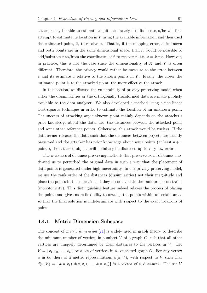
Chapter 4. Evaluation of Privacy and Information Loss 91
attacker may be able to estimate x quite accurately. To disclose x, s/he will first
attempt to estimate its location in Y using the available information and then used
the estimated point, x, to resolve x. That is, if the mapping error, ε, is known
and both points are in the same dimensional space, then it would be possible to
add/subtract ε to/from the coordinates of x to recover x, i.e. x = x± ε. However,
in practice, this is not the case since the dimensionality of X and Y is often
different. Therefore, the privacy would rather be measure as the error between
x and its estimate x relative to the known points in Y . Ideally, the closer the
estimated point is to the attacked point, the more effective the attack.
In this section, we discuss the vulnerability of privacy-preserving model when
either the dissimilarities or the orthogonally transformed data are made publicly
available to the data analyser. We also developed a method using a non-linear
least-squares technique in order to estimate the location of an unknown point.
The success of attacking any unknown point mainly depends on the attacker’s
prior knowledge about the data, i.e. the distances between the attacked point
and some other reference points. Otherwise, this attack would be useless. If the
data owner releases the data such that the distances between objects are exactly
preserved and the attacker has prior knowledge about some points (at least n+ 1
points), the attacked objects will definitely be disclosed up to very low error.
The weakness of distance-preserving methods that preserve exact distances mo-
tivated us to perturbed the original data in such a way that the placement of
data points is generated under high uncertainty. In our privacy-preserving model,
we use the rank order of the distances (dissimilarities) not their magnitude and
place the points in their locations if they do not violate the rank order constraint
(monotonicity). This distinguishing feature indeed relaxes the process of placing
the points and gives more flexibility to arrange the points within uncertain areas
so that the final solution is indeterminate with respect to the exact locations of
points.
4.4.1 Metric Dimension Subspace
The concept of metric dimension [71] is widely used in graph theory to describe
the minimum number of vertices in a subset V of a graph G such that all other
vertices are uniquely determined by their distances to the vertices in V . Let
V = {v1, v2, . . . , vn} be a set of vertices in a connected graph G. For any vertex
u in G, there is a metric representation, d(u, V ), with respect to V such that
d(u, V ) = {d(u, v1), d(u, v2), . . . , d(u, vn)} is a vector of n distances. The set V

Chapter 4. Evaluation of Privacy and Information Loss 92
is called a resolving set [23, 93] for G if and only if, for any vertex w, d(w, V ) =
d(u, V ), which implies that w = u for all pairs w and u of vertices in G. The metric
dimension, denoted by dim(G), is the minimum cardinality of the resolving set V
for G.
The above results of metric dimension in graph theory can be generalised for
any metric space in Rn. That is, the metric dimension of any given metric space
is the smallest number of points such that every point of the space is uniquely
determined by their distances to the chosen points. Let dij = ||xi − xj|| be the
Euclidean distance between points xi ad xj in data X, where X ∈ Rn. Given a
set of n + 1 known points (also known as references), we can find the location
of any point x ∈ X, by measuring the distance from x to each point in the set
of known points. The subspace of n + 1 points is called a metric dimension. To
mathematically define the metric space, we should first define the notion of a
resolving set as follows:
Definition 4.1 (Resolving Set). Let (X, d) be a metric space. A finite subset
{x1, x2, . . . , xn} ⊆ X is a resolving set for X if and only if for every point y ∈ X,
the list of distances
d(y, x1), d(y, x2), . . . , d(y, xn)
is unique.
The metric dimension can then be defined as follows:
Definition 4.2 (Metric Dimension). Let V be a resolving set for X, the metric
dimension, dim(X), is the smallest size of V .
Any n-dimensional data can be understood as a set of points in n-dimensional
Euclidean space. Therefore, all Euclidean distance-related concepts we defined
earlier in Chapter 2 can be applied and measured on (X, d). Additionally, since
the estimation of the location for any given point, x, depends on minimising the
relative error, it would be appropriate here to defined so called resolving function
[47].
Definition 4.3 (Resolving Function). A function f : X → [0, 1] is a resolving
function of the metric space (X, d) if and only if∑
[z∈X, d(x,z)6=d(y,z)] f(z) ≥ 1 for
any distinct points x, y ∈ X.
The fractional resolving dimension of (X, d) is F = min∑
x∈X g(x) where g
is a minimal resolving function of X and the minimum is taken over resolving
functions f such that any function f ′ with f ′ ≤ f and f ′ 6= f is not resolving.

Chapter 4. Evaluation of Privacy and Information Loss 93
1r
2r
3r
x
1xrd3xrd
2xrd
Figure 4.6: Trilateration example in 2-dimensional space.
Since the perturbed space, Y , generated by the non-metric MDS is an ε-
isometric space by definition (2.5), estimating the locations of points will always be
erroneous. That is, to provide a maximum privacy guarantee, we use non-metric
MDS perturbation in order to inject some distance distortion to the perturbed
space so that any distance-based attack will fail to accurately find unknown points.
Trilateration [20] is an iterative method applied to solve non-linear equations
in order to minimise the uncertainty of estimating the exact location in a metric
dimension. It is widely used in satellite navigation [114], robot localisation [162]
and network topology [142]. It is sometime called Multilateration when more than
three reference points are used to position the object. Here in this section, we use
the term “Multilateration”. The basic idea behind Multilateration is to determine
absolute or relative locations of points by measuring the distances between these
points and other known points, using the geometry of circles for 2-dimensional
space, R2, or the geometry of spheres for higher dimensions, Rn, where n > 2.
Multilateration differs from Triangulation in that it does not use triangle geometry
in determining the location of any given point. In Triangulation, the location of
the point is determined by measuring angles to it from known points at either end
of a fixed baseline, rather than measuring distances to the point directly so that
the point can then be located as the third point of a triangle with one known side
and two known angles.
Figure 4.6 shows an example of Trilateration, which utilises three references,
r1, r2 and r3, to calculate the position of unknown point, x, in R2. Intuitively, the

Chapter 4. Evaluation of Privacy and Information Loss 94
point x should be located at the intersection of the three circles centred at each
reference.
4.4.2 Distance-Based Attack Algorithm
Assume that the attacker knows n+1 points in the original data and their distances
to an attacked point, x. To attack x in the perturbed data, Y , the attacker can
use the available distances to estimate the location of the point x by choosing any
random point in Y to be x and iteratively improving the distance measurements
from x to the n+1 known points until they become the same as the real distances.
That is, the problem of estimating the location of a given point can be seen as
optimisation problem and we hope to minimise the sum of squared error using
either linear or non-linear least-squares method [124]. In this section, we use the
non-linear least-squares method to find the minimiser of the optimisation function
as well as measure the relative error of locating the unknown point.
4.4.2.1 Non-linear Least-squares Method
Suppose X ∈ Rn is an m×n data matrix, and we want to find the location of an un-
known point, x, given a set of n+1 known reference points, R = {r1, r2, . . . , rn+1}.Let dxri be the true Euclidean distance from point x and each reference point ri,
dxri = ||x− ri|| =
√√√√ n∑k=1
(xk − rik)2, (4.12)
where xk and rik are the kth dimension of x and ri, respectively.
The location of points x is determined by minimising the sum of squares on
distances,
G(x) =n+1∑i=1
gi(x)2, (4.13)
where
gi(x) =√
(x1 − xi1)2 + (x2 − xi2)2 + . . .+ (xn − xin)2 − dxri (4.14)
is a non-linear function of n variables representing the coordinates of point x.
That is, we choose estimates x1, x2, . . . , xn that minimise G(x). The quantity√(x1 − xi1)2 + (x2 − xi2)2 + . . .+ (xn − xin)2 is the measured Euclidean distance

Chapter 4. Evaluation of Privacy and Information Loss 95
from point x and each reference point ri. To solve this problem and find the
minimum of the sum of squares, we use Gauss-Newton method which starts with
a guess for x and iteratively moves toward a better solution along the gradient of
G(x) until convergence.
If g(x) is differentiable, then the refinement of point x at iteration k can be
achieved by the following linear approximation:
g(x) ≈ g(xk) +∇g(xk)T (x− xk), (4.15)
where
∇G(xk) =
∂g1(x)∂x1
∂g1(x)∂x2
. . . ∂g1(x)∂xn
∂g2(x)∂x1
∂g2(x)∂x2
. . . ∂g2(x)∂xn
...... . . .
...
∂gn+1(x)∂x1
∂gn+1(x)∂x2
. . . ∂gn+1(x)∂xn
, (4.16)
is the gradient (Jacobian) matrix that composes all first derivatives of x. Let
Ak =
∇g1(xk)
∇g2(xk)
...
∇gn+1(xk)
and bk =
∇g1(xk)Txk − g1(xk)
∇g2(xk)Txk − g2(xk)
...
∇gn+1(xk)Txk − gn+1(xk)
.
To find xk+1 from xk, we should minimise the sum of the squares of the linearised
residuals, i.e.
n+1∑i=1
(gi(x
k) +∇gi(xk)T (x− xk))2
, (4.17)
which is equivalent to solving the system Akx − bk = 0 which is defined by
(Ak)TAkx = (Ak)T bk and always consistent even when Akx = bk is not consis-
tent [118]. If Ak is non-singular, then there is a unique solution for x, which

Chapter 4. Evaluation of Privacy and Information Loss 96
represents the new position for the point x. The new position is given by
xk+1 = ((Ak)TAk)−1(Ak)T b. (4.18)
WhenG(xk) = 0, then the point xk+1 is a global minimum and we stop searching
the solution space. Otherwise, we move one step ahead.
The point xk+1 represents a further movement relative to the previous position,
xk, and towards better location such that the error is minimised. Intuitively, the
quality of the new position, xk+1, depends on how far away the point xk+1 is from
the real position of the point x at any iteration k. This is equivalent to minimising
(4.13). Another possible way to measure the relative distance error is to minimise
the normalised sum of squares, i.e.
n+1∑i=1
(||xk − ri|| − dxri||xk − ri||
)2
, (4.19)
where ||xk−ri|| is the measured Euclidean distance from point x and each reference
point ri at the kth iteration.
Finally, the accuracy of the estimation for any attacked point can be assessed by
computing the residual value between the estimated, x, and the real, x, locations,
i.e. ||x− x||.
4.4.2.2 Point Location Estimation using a Set of Distances
In this section, we simulate a location attack of any given unknown point using
a simple search algorithm that can estimate the location of the unknown point
while minimising the sum of least-squares as described in the previous section.
The main steps are as follows: start with an initial guess and move around in the
direction where the relative error is minimised. The process is then repeated until
convergence as described in Algorithm 4.2. The algorithm requires O((n+ 1)2m)
assuming that m > n+ 1 where m is the number of points and n is the number of
dimensions.
The algorithm operates on the perturbed data, Y , and starts by estimating
the location of the unknown point with the maximum number of known points.
Notice that the large the number of known references, the better accuracy and the
faster convergence could be achieved. Once the position of the unknown point is
estimated, it is then compared with its exact location in the perturbed data and
then the relative error is computed.

Chapter 4. Evaluation of Privacy and Information Loss 97
Algorithm 4.2 Distance-Based Attack Algorithm
Input: A set of n+1 known points, r1, r2, . . . , rn+1, an initial guess, x0, a tolerance,t > 0, and a maximum number of iterations, maxItr.
Output: An estimation, x, of the unknown point, x.1: repeat2: Calculate n+ 1 distances, dxr1 , dxr2 , . . . , dxrn+1 , from the current xk to each
reference point, r.3: Evaluate gi(x
k) and ∇gi(xk) for i = 1, 2, . . . , n+ 1.4: Move xk a bit towards better location along the gradient,
xk+1 = ((Ak)TAk)−1(Ak)T b.5: Calculate the error, err.6: until the error becomes less than the tolerance, err < t, or maximum number
of iterations is exceeded, k > maxItr.
Figure 4.7: 95% confidence ellipse to show the effect of outliers on pointlocation estimation. The outliers are distinguished by red circles. The open
circle is the data mean.
Although, in most cases, the accuracy of estimating a given unknown point
can be very high, the non-linear least-squares method is sensitive to outliers [50].
Reference points measured with abnormally smaller or larger distances from the
unknown point can be considered as outliers. That is, when the estimated points
largely diverges from the data mean value, the variance of the estimator becomes
higher reducing the accuracy of the algorithm. Figure 4.7 illustrates the effect of
outliers on location estimation. The convex shape of variance ellipse with 95%
confidence interval changes whenever the number of outliers increase. Another
drawback of such method is that the performance often depends on the choice of

Chapter 4. Evaluation of Privacy and Information Loss 98
the initial estimates as a bad choice would lead to too slow convergence or to an
estimation with high bias.
4.4.2.3 Numerical Example
To illustrate the process of locating an unknown point x, consider the following
example in 2-dimensional space. Assume that we want to estimate the location
of a point, x, where x = (1, 1), using some other known points. Without loss of
generality, we assume that the real location, i.e. (1, 1), of the point x is unknown
to the attacker and the only available information are the three reference points
and their distances to the point x. Let r1 = (1, 3), r2 = (2,−3) and r3 = (−2, 3)
be three known reference points. Assume that the distances from the unknown
point, x, and these point are dxr1 = 2, dxr2 = 4.12 and dxr3 = 3.61. Assume also
that the tolerance is set to 0.01. Let us now define three functions in two variables
x1 and x2
g1(x1, x2) =√
(1− x1)2 + (3− x2)2 − dxr1=
√(1− x1)2 + (3− x2)2 − 2 = 0,
g2(x1, x2) =√
(2− x1)2 + (−3− x2)2 − dxr2=
√(2− x1)2 + (−3− x2)2 − 4.12 = 0,
g3(x1, x2) =√
(−2− x1)2 + (3− x2)2 − dxr3=
√(−2− x1)2 + (3− x2)2 − 3.61 = 0,
where x1 and x2 are the coordinates of point x and we hope to minimise the sum
of squares, i.e.
3∑i=1
gi(x1, x2)2.
Let (0, 0) be an initial start point and iteratively evaluate ∇gi(x1, x2). The
solution converges in 12 iterations at point (0.9977, 0.9913) with an error equal
to 0.009. Figure 4.8 depicts the results. Similarly, If we started with a random
initial point, we could find an estimation of point x at (1.0069, 0.9959) after 14
iterations; and with an error equal to 0.008. The results are shown in Figure 4.9.
4.4.3 Disclosure Risk Measure
The disclosure risk can be defined as the ability that the attacker has to easily
identify the exact location of a given unknown point or a sets of unknown points.
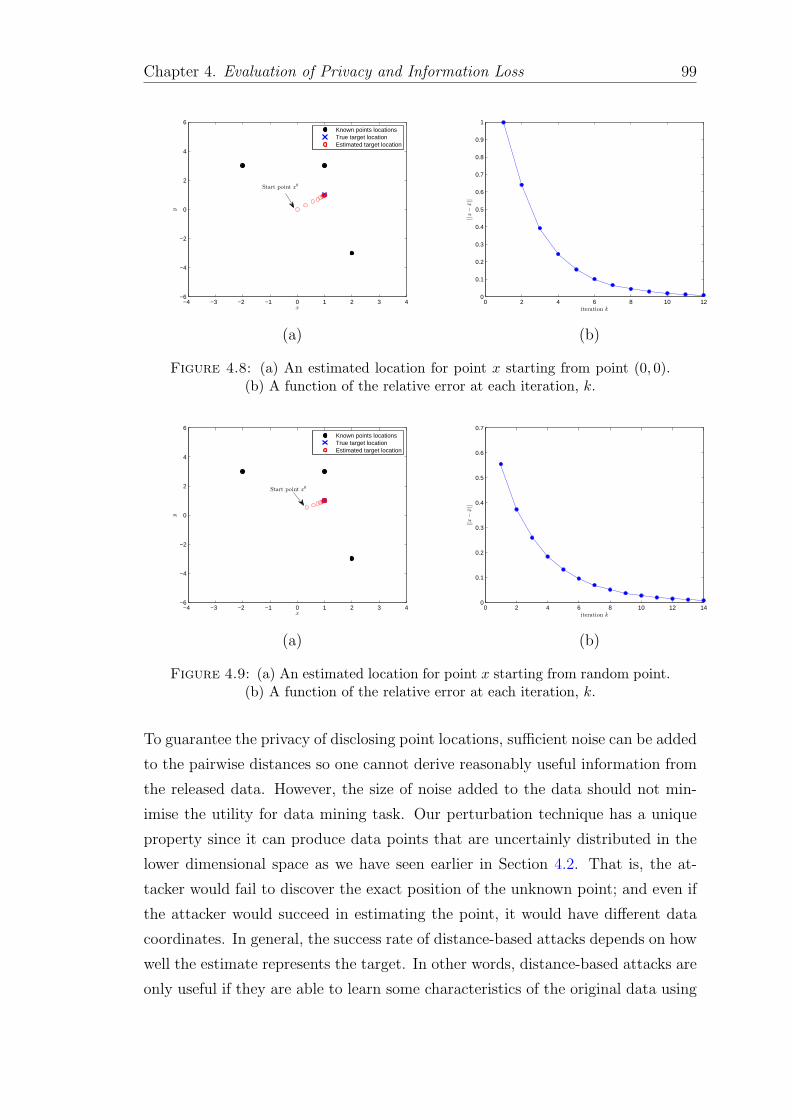
Chapter 4. Evaluation of Privacy and Information Loss 99
−4 −3 −2 −1 0 1 2 3 4−6
−4
−2
0
2
4
6
x
y
Known points locationsTrue target locationEstimated target location
Start point x0
0 2 4 6 8 10 120
0.1
0.2
0.3
0.4
0.5
0.6
0.7
0.8
0.9
1
iteration k
||x−
x||
(a) (b)
Figure 4.8: (a) An estimated location for point x starting from point (0, 0).(b) A function of the relative error at each iteration, k.
−4 −3 −2 −1 0 1 2 3 4−6
−4
−2
0
2
4
6
x
y
Start point x0
Known points locationsTrue target locationEstimated target location
0 2 4 6 8 10 12 140
0.1
0.2
0.3
0.4
0.5
0.6
0.7
iteration k
||x−
x||
(a) (b)
Figure 4.9: (a) An estimated location for point x starting from random point.(b) A function of the relative error at each iteration, k.
To guarantee the privacy of disclosing point locations, sufficient noise can be added
to the pairwise distances so one cannot derive reasonably useful information from
the released data. However, the size of noise added to the data should not min-
imise the utility for data mining task. Our perturbation technique has a unique
property since it can produce data points that are uncertainly distributed in the
lower dimensional space as we have seen earlier in Section 4.2. That is, the at-
tacker would fail to discover the exact position of the unknown point; and even if
the attacker would succeed in estimating the point, it would have different data
coordinates. In general, the success rate of distance-based attacks depends on how
well the estimate represents the target. In other words, distance-based attacks are
only useful if they are able to learn some characteristics of the original data using

Chapter 4. Evaluation of Privacy and Information Loss 100
the perturbed.
To show how our privacy-preserving model would be resistant to distance-based
attacks, let us go back to the previous 2-dimensional example. We perturbed all
the three known points, r1, r2, r3, and the unknown point, x. For easy visualisation,
we kept the dimensions of the perturbed data the same as the original dimensions,
i.e. 2-dimensions. Table 4.1 shows both the original and perturbed data values.
The distances difference (stress) between points in the original and the perturbed
space was 8.34 × 10⁻⁸. Assume that the attacker knows the points r1, r2 and r3
in the perturbed data and their distances to the unknown point x as well. The
attacker can accurately estimate the location of point x up to a very small error.
The estimated point was at (0.44, 0.0007) which is quite near to the point x in the
perturbed data and the error was just 0.00036. If the attacker knows the mapping
error, it would be possible to estimate the position of the point in the original data,
particularly if both the original and perturbed data lie in the same dimensional
space. Figure 4.10 shows the data points in the original and perturbed spaces.
Note that the distances between points have shrunk because we normalised the
original data before the perturbation. The Euclidean distance, ||x− x||, from the
point x in the original data, X, to the estimated point x in the perturbed data,
Y , can be also used as a measure to quantify the privacy of our model. That is,
the large the distance, the better the privacy is preserved.
Table 4.1: Original and perturbed data values.
Original data Perturbed datax1 x2 x1 x2
r1 1 3 1.45 0.003r2 2 -3 -0.94 -1.40r3 -2 1 -0.95 1.40x 1 1 0.44 0.00034
Recall that any individual data object is said to be disclosed if it is on a very
close distance from its estimate. Another quantitative method to measure how
close the estimated point is from the target point, would be to compute the ratio
of the differences between x and its estimate x to the average distance from x to
the n+ 1 known points r1, r2, . . . , rn+1, i.e.
ρ∗ =||x− x||
1n+1
∑n+1j=1 ||x− rj||
. (4.20)
The overall privacy is then given by
Chapter 4. Evaluation of Privacy and Information Loss 101
−3 −2 −1 0 1 2 3−4
−3
−2
−1
0
1
2
3
4
r1
r2
r3 x
x
Original data XPerturbed data Y
Figure 4.10: Data points in the original space, X, and the perturbed space,Y . The dashed line are the Euclidean distances.
ρ =1
N
N∑i=1
||xi − xi||1
n+1
∑n+1j=1 ||xi − rj||
, (4.21)
where N is the number of the remaining unknown points.
This measure provides precise upper bounds on the privacy guarantee of the
original data, X, in terms of the norms of the Euclidean distances between data
objects. The lower value of ρ gives the data owner the worst case privacy assurance
since the inference of any attacked point would occur if its estimate is located on
very close distance. Hence, the larger the value of ρ, the greater the privacy.
4.4.4 Experiments
In this section, we empirically evaluate the effectiveness of distance-based attack
in disclosing the original data values on both synthetic and real datasets. The
attack was implemented using Matlab 7.0. For the synthetic data, we generated
m random objects in n dimensional space where m = 1000 and n = 100. That
is, we should solve a system with 100 variables and ensure that the placement
of unknown points can be accurately calculated. We randomly chose n + 1 to
be known points and tried to find an unknown point chosen randomly from the
remaining (m−(n+1)) data points. For simplicity, we set up the maximum number
of iterations to 100 and carried out this process 100 times. To see the impact of
data perturbation on the accuracy of estimating the location of an unknown point

Chapter 4. Evaluation of Privacy and Information Loss 102
0 20 40 60 80 100
0.04
0.05
0.06
0.07
0.08
0.09
0.1
0.11
||x−
x||
(a)
10 20 30 40 50 60 70 80 90
0.025
0.03
0.035
0.04
0.045
0.05
0.055
0.06
0.065
#Dimensions
||x−
x||
(b)
Figure 4.11: (a) Average error (red line) of distance-based attack in locatingunknown point x in the perturbed data, Y along with the lower and upperbounds (blue lines). (b) Average error of estimating the location of an unknown
point, x, at different dimensions in Y .
in the perturbed data, we transformed the data into 9 different lower dimensional
spaces using non-metric MDS. Then, we conduct a distance-based attack on each
perturbed dataset. Figure 4.11(a) shows the results averaged over 100 runs on
the perturbed data at the 90-dimensions space. The average change in distances
(stress) between the original and perturbed data caused by the perturbation was
0.0088, which is relatively low. Note that the size of change in distance can be
understood as noise that would effect the performance of distance-based attack, i.e.
a high level of noise will have large effect in downgrading the accuracy of estimating
the location of unknown points. Figure 4.11(b) shows the relative errors of the
attack at different dimensions. The results suggest that using non-metric MDS
successfully increases the uncertainty of locating points in the perturbed space.
They also suggest that transforming the data into a lower dimensionality than
the original data but preserving as many dimensions as possible, produces more
privacy preservation as the estimation error substantially increases, e.g. n = 70,
n = 80 and n = 90. This is because of geometric distortion of positional relations
in the higher dimensional space due to the monotonicity restriction applied in the
perturbation as described in Section 4.2.
We also evaluated the effectiveness of the attack on 15 real numeric datasets
taken from the UCI machine learning repository [58]. The description of the
datasets are shown Table 4.2. To assess the privacy of the data, we systematically
reduced the dimensions of the data using five different techniques (RP [110, 129],

Chapter 4. Evaluation of Privacy and Information Loss 103
Table 4.2: Benchmark datasets used in our experiments.
Dataset # Records # Attributes
Breast Cancer Wisconsin (BCW) 699 9Credit Approval 690 14Pima Diabetes 768 8Hepatitis 155 19Iris 150 4Wine 178 13Handwritten Digits 3823 64Ecoli 336 7Image Segementation 2100 19Multiple Features 2000 216Page Blocks 5473 10Spambase 4601 57Synthetic Control Chart (SCC) 600 60Yeast 1484 8Satlog 2000 36
PCA [11], SVD [178], non-metric MDS (NMDS) and DCT [121]) and attempted
to estimate the locations of the unknown points. To show how much information
is lost as a result of the transformation, we computed the stress (4.3) at each
dimension. Figure 4.12 shows a comparison of the average privacy at different
dimensions, calculated over 20 trials, plotted versus the stress. Interestingly, all
methods exhibit a resistance to the attack. However, NMDS gives much higher
privacy than other methods, particularly at the high dimensions. Although NMDS
outperforms all other methods, the performance of NMDS and DCT was quite
similar in most cases. Similarly, the performance of attack on the data generated
by both PCA and SVD was also quite similar at all dimensions. It can also
be seen that RP performs worse than any other methods. This is probably due
to the orthogonal linear transformation applied on the data which preserves the
inner product and thus the Euclidean distances among the data objects are still
maintained. On the other hand, the stress is low at the higher dimensions and
high at the low dimensions. This confirms that transforming data into the high
dimensions always gives the best fit of data for distance-based analysis. The value
of stress for NMDS is very low for all datasets compared with other methods,
which indicates that the pairwise distance between points in the perturbed data,
Y , is well preserved.
Our experimental results show that including a large number of features in the
perturbed data is sufficient to maintain high data utility and privacy against the

Chapter 4. Evaluation of Privacy and Information Loss 104
distance-based attack. This implies a win-win situation as the trade-off between
privacy and utility is not obvious. In some applications when determining the
location of the points is a privacy concern (e.g. mobile devices location tracking
[112]), the data owner may wish to project the data into higher dimensions in
which the precision of distance-based attack can sufficiently be reduced.
In another set of experiments, we incrementally varied the number of the known
points to see its effect on the accuracy of locating unknown points. We transformed
four datasets into six different dimensions and at each dimension we used different
numbers of known points. The average privacy calculated over 20 replications is
shown in Figure 4.13. The results indicate that the estimation error decreases as
the number of known points increases. This implies that when a sufficient number
of known points is available to the attacker, the accuracy of the estimation is
improved. The results also confirm that the error of determining the location of
an unknown point increases when the number of dimensions increases. Again,
we conclude that transforming the data into the few lower dimensions from the
original dimensionality gives reasonable utility and privacy.
Distance-based attack naively assumes that none of the measured distances are
outliers. Therefore, it would produce highly accurate estimation. However, if some
of the reference points are located at a long distance away from the attacked point,
the estimation would result in greater error. To test the attack in the presence
of outliers, we use the same synthetic data generated in the above experiment;
and for comparison, we experiment four different sizes of outliers—1%, 5%, 10%
and 15%. In this experiment, we define an outlier as any data object that is
above or below three standard deviations. Each set of the outliers is included
within the n+ 1 known points which are then used to disclose the location of the
attacked point. The experiment has been repeated 20 times and the results are
then averaged. Figure 4.14 shows the estimation error for each case at different
iterations, k. The distances between points become heavily dominated by noise as
the outliers increases. That can be clearly observed during the first few iterations.
The quality of the location estimation depends on the relative noise contained
in the data. As the noise added to the data increases, the estimation accuracy
decreases. In general, the effect of noise caused by outliers will mainly affect
location estimates, particularly when the data are small. Consequently, if the
attacker has some knowledge about the outliers, she would eliminate them from
the data or discard points with the largest studentised residuals so that the largest
advantages of the attack could be reached.

Chapter 4. Evaluation of Privacy and Information Loss 105
Finally, we conducted an experiment to demonstrate how our perturbation
method would be resistant to the attack when the attacker has prior knowledge
about both the dimensionality of the original data and the type of transformation,
which is distance-preserving. We perturbed the original data, X, into different
dimensional spaces. The stress was 0.3849, 0.2654, 0.1688, 0.1218, 0.0918, 0.0702,
0.0536, 0.0401, 0.0285, 0.013 for dimensions 5, 10, 20, 30, 40, 50, 60, 70, 80 and
90, respectively. To find a good approximation of X, we develop a simple but
effective method to reverse back the transformation and up-scale the perturbed
data, Y , to its original dimensional space. To apply the attack, the attacker can
pad the perturbed data Y with a set of features in order to achieve the full n
dimensions. We generated three sets of features: a set of zero-valued features, a
set of random features and a set of random features that have average distance
equal to the average dissimilarity. We then measure how far the estimated data,
X, are from the original data, X. Let Y = [Y1, Y2, . . . , Yp] be an m × p matrix
representing the perturbed data and V = [V1, V2, . . . , Vn−p] be a set of the new
features. To produce an estimation, X, of data X, we expand the size of the
dimensions of data matrix Y by combing the features of V and generate an m×nmatrix X, i.e. X = [Y1, Y2, . . . , Yp, V1, V2, . . . , Vn−p]. Note that the new added zero-
valued features count nothing to the objects’ pairwise distance so the distances
are kept unchanged and some good fitting of data X can then be achieved. This
is a quite similar to the classical metric MDS solution which often converges to a
local optimum in one step as described earlier in Chapter 3. The random features,
on the other hand, will indeed introduce more distortion to the pairwise distance,
but the features that preserve the average distance my provide to some extent a
good approximation of the original features.
The inference may then occur if the attacker finds any data object in data
X that is very close to its estimate, i.e. ||x − x|| is minimised. The overall
average privacy of the perturbed data are depicted in Figure 4.15. For zero-valued
features, as the number of dimension increases, the privacy increases. In contrast,
for the random features, as the number of added random features increases, the
distance deviation increases because the size of noise is increased as well, causing
more distortion. The features with average distance demonstrate low privacy
preservation as the error is slightly decreased. Here, we can say that there is a
trade-off between the number of added features and the effectiveness of the attack.

Chapter 4. Evaluation of Privacy and Information Loss 106
87654320
0.1
0.2
0.3
0.4
0.5
0.6
0.7
0.8
0.9
1
Number of dimensions (p)
Avg
.P
riva
cy(ρ
)
Breast Cancer Wisconsin
RPPCASVDNMDSDCT
0
0.1
0.2
0.3
0.4
0.5
0.6
0.7
0.8
0.9
1
Stre
ss(S
)
121110987654320
0.1
0.2
0.3
0.4
0.5
0.6
0.7
0.8
Number of dimensions (p)
Avg
.P
riva
cy(ρ
)
Credit Approval
RPPCASVDNMDSDCT
0
0.1
0.2
0.3
0.4
0.5
0.6
0.7
0.8
0.9
1
Stre
ss(S
)
320
0.1
0.2
0.3
0.4
0.5
0.6
0.7
0.8
Number of dimensions (p)
Avg
.P
riva
cy(ρ
)
Iris
RPPCASVDNMDSDCT
0
0.1
0.2
0.3
0.4
0.5
0.6
0.7
0.8
0.9
1
Stre
ss(S
)
21520017515012510075502510520
0.1
0.2
0.3
0.4
0.5
0.6
0.7
0.8
0.9
1
Number of dimensions (p)
Avg
.P
riva
cy(ρ
)
Multiple Features
RPPCASVDNMDSDCT
0
0.1
0.2
0.3
0.4
0.5
0.6
0.7
0.8
0.9
1
Stre
ss(S
)
181512107520
0.1
0.2
0.3
0.4
0.5
0.6
0.7
0.8
0.9
Number of dimensions (p)
Avg
.P
riva
cy(ρ
)
Image Segementation
RPPCASVDNMDSDCT
0
0.1
0.2
0.3
0.4
0.5
0.6
0.7
0.8
0.9
1
Stre
ss(S
)
5040302010520
0.1
0.2
0.3
0.4
0.5
0.6
0.7
0.8
0.9
Number of dimensions (p)
Avg
.P
riva
cy(ρ
)
Spambase
RPPCASVDNMDSDCT
0
0.1
0.2
0.3
0.4
0.5
0.6
0.7
0.8
0.9
1
Stre
ss(S
)
181512107520
0.1
0.2
0.3
0.4
0.5
0.6
0.7
0.8
Number of dimensions (p)
Avg
.P
riva
cy(ρ
)
Hepatitis
RPPCASVDNMDSDCT
0
0.1
0.2
0.3
0.4
0.5
0.6
0.7
0.8
0.9
1
Stre
ss(S
)
654320
0.1
0.2
0.3
0.4
0.5
0.6
0.7
0.8
Number of dimensions (p)
Avg
.P
riva
cy(ρ
)
Ecoli
RPPCASVDNMDSDCT
0
0.1
0.2
0.3
0.4
0.5
0.6
0.7
0.8
0.9
1
Stre
ss(S
)
121110987654320
0.1
0.2
0.3
0.4
0.5
0.6
0.7
0.8
Number of dimensions (p)
Avg
.P
riva
cy(ρ
)
Wine
RPPCASVDNMDSDCT
0
0.1
0.2
0.3
0.4
0.5
0.6
0.7
0.8
0.9
1
Stre
ss(S
)
63605040302010520
0.1
0.2
0.3
0.4
0.5
0.6
0.7
0.8
0.9
Number of dimensions (p)
Avg
.P
riva
cy(ρ
)
Handwritten Digits
RPPCASVDNMDSDCT
0
0.1
0.2
0.3
0.4
0.5
0.6
0.7
0.8
0.9
1
Stre
ss(S
)
7654320
0.1
0.2
0.3
0.4
0.5
0.6
0.7
Number of dimensions (p)
Avg
.P
riva
cy(ρ
)
Yeast
RPPCASVDNMDSDCT
0
0.1
0.2
0.3
0.4
0.5
0.6
0.7
0.8
0.9
1
Stre
ss(S
)
353025201510520
0.1
0.2
0.3
0.4
0.5
0.6
0.7
0.8
0.9
Number of dimensions (p)
Avg
.P
riva
cy(ρ
)
Satlog
RPPCASVDNMDSDCT
0
0.1
0.2
0.3
0.4
0.5
0.6
0.7
0.8
0.9
1
Stre
ss(S
)
987654320
0.1
0.2
0.3
0.4
0.5
0.6
0.7
0.8
0.9
Number of dimensions (p)
Avg
.P
riva
cy(ρ
)
Page Blocks
RPPCASVDNMDSDCT
0
0.1
0.2
0.3
0.4
0.5
0.6
0.7
0.8
0.9
1
Stre
ss(S
)
5040302010520
0.1
0.2
0.3
0.4
0.5
0.6
0.7
0.8
Number of dimensions (p)
Avg
.P
riva
cy(ρ
)
SCC
RPPCASVDNMDSDCT
0
0.1
0.2
0.3
0.4
0.5
0.6
0.7
0.8
0.9
1
Stre
ss(S
)
7654320
0.1
0.2
0.3
0.4
0.5
0.6
0.7
0.8
Number of dimensions (p)
Avg
.P
riva
cy(ρ
)
Pima−indian−diabets
RPPCASVDNMDSDCT
0
0.1
0.2
0.3
0.4
0.5
0.6
0.7
0.8
0.9
1
Stre
ss(S
)
Figure 4.12: Average privacy (ρ) against distance-based attack versus stress(S) at different dimensions using different perturbation techniques. The bold
line is stress and the dashed line is average privacy.

Chapter 4. Evaluation of Privacy and Information Loss 107
1 2 3 4 5 60
0.5
0.6
0.65
0.7
0.75
0.8
Dimension Difference (n− p)
Avg
.P
riva
cy(ρ
)
Breast Cancer Wisconsin
n+1 known pointsn+3 known pointsn+6 known pointsn+9 known points
(a)
1 2 3 4 5 60
0.1
0.2
0.3
0.4
0.5
0.6
0.7
0.8
0.9
1
Dimension Difference (n− p)
Avg
.P
riva
cy(ρ
)
Credit Approval
n+1 known pointsn+3 known pointsn+6 known pointsn+9 known points
(b)
1 2 3 4 5 60
0.05
0.1
0.15
0.2
0.25
0.3
0.35
Dimension Difference (n− p)
Avg
.P
riva
cy(ρ
)
Pima−indian−diabets
n+1 known pointsn+3 known pointsn+6 known pointsn+9 known points
(c)
1 2 3 4 5 60
0.1
0.2
0.3
0.4
0.5
0.6
0.7
0.8
0.9
Dimension Difference (n− p)
Avg
.P
riva
cy(ρ
)
Hepatitis
n+1 known pointsn+3 known pointsn+6 known pointsn+9 known points
(d)
Figure 4.13: Average privacy (ρ) against distance-based attack at differentdimensions using different numbers of the known points.
0 20 40 60 80 1000
0.1
0.2
0.3
0.4
0.5
0.6
0.7
0.8
0.9
1
iteration k
||x−
x||
1% noise5% noise10% noise15% noise
Figure 4.14: Estimated loca-tion error at different iterations,k, using different sizes of noisymeasures for the n + 1 known
points.
5 10 20 30 40 50 60 70 80 900.4
0.5
0.6
0.7
0.8
0.9
1
1.1
# Dimensions
||x−
x||
Zero UpscalingRandom UpscalingDistance−Preserving Random Upscaling
Figure 4.15: Estimated errorat different dimensions, p, usingzero-valued features up-scaling,random-valued features up-scaling and distance-preserving
features up-scaling.

Chapter 4. Evaluation of Privacy and Information Loss 108
4.5 PCA-Based Attack
PCA basically reduces the dimensions of the data according to the number of
principal components that retain a sufficient amount of variation. Computation-
ally, this can be achieved by multiplying the data matrix with an orthogonal
matrix containing the eigenvectors of the covariance matrix, arranged in columns
in descending order of the corresponding eigenvalues. The number of eigenvectors
determines the number of dimensions that the data should have in the new space.
In the context of PPDM, PCA can be used as a tool to reconstruct the behaviour
of the original data if certain information (known sample) or knowledge about the
data is available to the attacker. The prior knowledge can be obtained through
direct or indirect access to the data. For instance, when private information of a
company can be disclosed by an in-house employee, that is a kind of direct access.
Whilst the indirect access involves the scenario when the underling distribution
of any unreleased data is learned from, for example, national statistical agencies
[165].
In this section, we generalise the PCA-based attack proposed in [108, 165] in
order to recover the original data from the perturbed data that are transformed
by arbitrary distance-preserving transformation, i.e. non-rigid motion transforma-
tion, ||xi − xj|| = ||T (xi) − T (xj)|| + eij where T is non-metric MDS and eij is a
small distortion error. The PCA-based attack mainly depends on the distribution
from which the original data are drawn. The basic idea behind the attack is to
map the perturbed data with the reference data (the original data) through the
computation of the eigen basis that span the known sample and the perturbed
data. Assume that the attacker has a collection of independent data samples,
S, from the same distribution from which the original data were drawn, X . To
recover the original data, the attacker will attempt to find a transformation that
composes a set of the eigenvectors obtained from both S and the perturbed data,
Y . Then s/he can project the data onto these eigenvectors such that the principle
directions of Y are aligned as much as possible with the principle directions of S.
4.5.1 Basics of PCA
In Section 2.6.2, we have briefly introduced the idea behind PCA. In this section,
we describe the concept of PCA in more detail to make it easier to follow the
attack. PCA is mainly used for two objectives. The first is reducing the number
of data variables while retaining the variability in the data as much as possible.

Chapter 4. Evaluation of Privacy and Information Loss 109
The second is discovering hidden patterns in the data since much of the noise
can be eliminated by choosing few variables [160]. When analysing a dataset
comprising of large number of variables, it is likely that subsets of variables are
highly correlated with each other. If two or more variables are strongly correlated,
it can be concluded that these variables are quite redundant and thus have the
same effect in defining the outcome of interest. For instance, suppose we have
measured the length and the width of a set of given shapes and assume that these
two variables seem to be positively correlated. Thus, we can replace them with a
single new variable, let say the area of the shape, that still captures most of the
information about the shape determined by its length and width.
PCA seeks a subspace that best preserves the variance of the data. The starting
point for PCA is the sample covariance or correlation matrix. Mathematically, it
finds a linear combinations of the variables that are mutually uncorrelated and
ordered in variance [86]. Let X be an m×n data matrix and ΣX be the covariance
matrix for X. The covariance of two variables Xi and Xj measures how strongly
the variables vary together. If i = j, then the covariance is just the variance of
the variable. If X is normalised, i.e. each variable in the data has zero-mean and
unit-variance, the covariance matrix is the dot product of X, ΣX = XTX. For
any data object x of n random variables in matrix X, the linear combinations can
be defined by
zk = ak1x1 + ak2x2 + . . .+ aknxn =n∑j=1
akjxj, (4.22)
where zk is the kth principle component (PC) and ak is an eigenvector of ΣX
corresponding to its kth largest eigenvalue λk. If ak is chosen to have unit length,
i.e. aTk ak = 1, then var(zk) = λk where var(zk) denotes the variance of zk. The
sum of the variance of PCs is equal to the sum of variance of X’s variables.
The goal of PCA is then to find an orthonormal basis (transformation) that
satisfies the following properties:
1. Each pair of new variables has zero covariance (for distinct variables).
2. The variables are ordered with respect to how much variance each variable
captures.
3. The first variable (PC1) captures as much variance as possible and the next
variable (PC2) captures as much of the remaining variance, and so on.

Chapter 4. Evaluation of Privacy and Information Loss 110
4. All PCs pass through the origin and they are all orthogonal to one another.
Let λ1, λ2, . . . , λn be the eigenvalues of ΣX . Since ΣX is semi-definite positive,
the eigenvalues are all non-negative and can be ordered such that λ1 ≥ λ2 ≥ . . . ≥λn−1 ≥ λn. Let U = [u1,u2, . . . ,un] be the matrix of eigenvectors of ΣX . The
eigenvectors are ordered so that the kth eigenvector corresponds to the kth largest
eigenvalue. Let X ′ = XU be the set of transformed data such that
var(X ′) = var(XU)
= E[(XU)T (XU)]
= E[UXXTUT ]
= UE[XTX]UT
= UAUT ,
(4.23)
where A is an n× n diagonal matrix containing the eigenvalues of ΣX .
The orthonormal basis U that maximises UAUT are the first eigenvectors of
U . The eigenvector associated with the largest eigenvalue indicates the direction
in which the data have the most variance. The eigenvector associated with the
second largest eigenvalue indicates the direction in which the data have the largest
remaining variance and it is orthogonal to that of the first eigenvector. Since the
projections are uncorrelated, the percentage of variance accounted for by retaining
the first p PC’s is given byPp
i=1 λiPni=1 λi
× 100. If all the n eigenvectors are used as a
transformation basis, then X ′ will be an exact match of X.
In summary, PCA can be viewed as a rotation of the original coordinate axes to
a new set of axes defined by the eigenvectors of ΣX and aligned with the variability
in the data. Although PCA is a powerful tool to preserve most of the variance,
it assumes the normality of the data and thus it may fail if the data lies on a
“complicated” manifold [34].
4.5.2 PCA-Based Attack Algorithm
The main reason to use PCA to attack our privacy model is to find a transformation
basis that aligns the principle components of the perturbed data with the principle
components of the original data. Assume that each data object, xi, in the original
data, X, is as an independent sample drawn from a random vector X with a

Chapter 4. Evaluation of Privacy and Information Loss 111
covariance matrix ΣX . The matrix ΣX is semi-definite positive and has non-
negative eigenvalues on diagonals. Assume also that the attacker has a set, S,
of k independent samples which are also drawn from X . Let {u1,u2, . . . ,un}be a set of orthogonal eigenvectors with associated eigenvalues {λ1, λ2, . . . , λn}of the symmetric matrix ΣX . The eigenspace can be defined by U = {ΣXui =
λiui : uTi uj = 0,ui,uj ∈ Rn}. Each eigenvector, ui, represents a line that can
be used as a basis to project the data onto it such that the resulting values would
have some amount of variance, λi. That is, for each ui, there are two possible
orientations, {ui,−ui}, such that the data are projected onto the subspace spanned
by one of these directions of ui. In other words, the eigenvectors can, for example,
be multiplied by -1 because if ΣXui = λiui, then ΣX (−1)ui = (−1)ΣXui =
λi(−1)ui = (−1)λiui, i.e. reflections of eigenvectors are admissible [118]. The
principal components are the new attributes generated from the projection onto
one or more of these eigenvectors.
Since both X and S independently arise from X , The covariance matrix, ΣS,
has the same eigenvectors as ΣX . It is easy to show that if ΣX and ΣS have
the same eigenvectors, their projections XUX and SUS are also the same [157].
To attack the perturbed data, Y , the attacker will assume that the distance is
completely preserved, i.e. ||xi − xj|| = ||T (xi) − T (xj)|| + eij where eij = 0, and
for the purpose of comparison, s/he will up-scale Y using zero-valued features
to produce X as estimation of X as described in Section 4.3. The attacker will
then try to match the principle components obtained from S with the principle
components from X. However, the projection of data along any eigenvector of the
covariance matrix would lead to different alignment of principle directions as there
are N = 2n possible principle alignments and thus we may end up with different
solutions [118].
To guarantee the best fit of the principle components for S and X, we use two-
sample hypothesis test to measure the equality of two distributions—the one from
the projections of S on US to the one from the projection of X on UX . Suppose
that {x1, x2, . . . , xn} and {y1, y2, . . . , yn} are two independent random samples of
random variables in Rn, with respective distributions F1 and F2 and we would like
to test the hypothesis that F1 is equal to a particular distribution F2, i.e. decide
between the following hypotheses:
H0 : F1 = F2 versus H1 : F1 6= F2.

Chapter 4. Evaluation of Privacy and Information Loss 112
If we fail to reject the null hypothesis (i.e. p-value > 0.05), then we conclude
that two samples come from the same distribution. Let F1(x) and F2(x) be the
cumulative distribution function of SU iS and XU i
X, respectively. To quantify the
distance between the two distribution functions, we use Kolmogorov-Smirnov test
[115] which is defined by
D = minx|F1(x) = F2(x)|. (4.24)
This test will be carried out for all the N possible principle directions and
the one that achieves the highest p-value will then be chosen. The steps of
the attack are described in Algorithm 4.3. The algorithm has O(n2m + n3 +
N(m logm)) computation complexity where finding all possible mirror images re-
quires O(N(m logm)) and computing the covariance matrices and the principle
components require O(n2m+ n3).
Algorithm 4.3 PCA-Based Attack Algorithm
Input: S set of k known independent samples drawn from a random variable, X ,data X, as an estimation of the original data, X.
Output: Recovered data, X ′.1: Up-scale the perturbed data, Y , to obtain an estimation, X, from X.2: Compute the covariance matrices ΣX from X and ΣS from S.3: Calculate the eigenvalues and their corresponding eigenvectors, UX and US.4: Search for all 2n possible mirror images of the eigenvectors and construct{U1
X, U2
X, . . . , UN
X} and {U1
S, U2S, . . . , U
NS }.
5: repeat6: Test the null hypothesis, H0 : F (SU i
S) = F (XU iX
).7: Choose the next principle direction alignment, i+ 1.8: until All N eigenvectors U i
Xand U i
S are examined.
9: Pick U i with highest p-value.10: Compute X ′ = XU i as the recover of X.
Our attack is to some extent similar to the attack proposed in [108]. However,
instead of exhaustively searching for a diagonal matrix A that introduces the best
matching between the eigenvectors for ΣS and ΣY , we directly search amongst
all directions to find the best orthogonal basis that keeps both distributions of
SU iS and XU i
Xclose to each other. Furthermore, they assume that the original
data objects are columns rather than rows as we assume; and to recover the
original data, they compute USAUTY Y . Another simple measure to find the best
eigenvectors’ mirrors is described in [165].

Chapter 4. Evaluation of Privacy and Information Loss 113
4.5.3 Distortion Quantification of Eigenstructure
Since the PCA-based attack is mainly based on the decomposition of the covari-
ance matrix, its robustness will then depend on the estimation of the covariance
matrix [108]. Non-metric MDS transformation perturbs covariance matrix esti-
mates significantly. In particular, the variance is inflated along the few first k
dimensions; insignificant dimensions may be added to the data and interesting
structures in the data may remain unrevealing [90]. The correlation structure
is also changed significantly as the new features, produced by non-metric MDS,
are uncorrelated and inconsistent with the correlation coefficients of the original
dimensions. That is, if the covariance matrix of the original data is unreliably
estimated, the performance of the attack will be significantly deteriorated.
As non-metric MDS perturbation changes the scale, represented by λ, and the
orientation, represented by U , the quality of analysing and matching the covariance
matrices for the known sample and the perturbed would be downgraded, i.e. λ+e
and U + E where e ∈ E is a small error such that 0 < e < 1. The impact of
non-metric MDS perturbation can be characterised in terms of the eigenspace of
the covariance matrix as follows:
1. The ratio of the largest and smallest eigenvalue of ΣY , λ1/λn, increases as
the largest eigenvalue, λ1, becomes very large or the smallest eigenvalue, λn,
becomes equal to zero. Note that the rank(ΣX) = rank(ΣX) − 1 because
the zero-valued features that are added to Y in order to estimate X count
nothing to the total variance in ΣY .
2. The eigenvectors order may be changed and consequently the subspace
spanned by the k first or the k last columns of UY is also changed. This
would introduce different PCs orientations and thus worse performance of
PCA-based attack in recovering the original data.
3. The matrix ΣX is semi-definite negative as it has n − p eigenvectors equal
to zero, i.e. ΣXui ≤ 0. This implies that ΣX has a null space, N(ΣX − λI),
and its is spanned by the eigenvectors associated with the eigenvalues that
are equal to zero.
The influence of non-metric MDS perturbation on both the eigenvalues’ scale
and the eigenvectors’ orientation of the covariance matrix for the known sample
with respect to the covariance matrix of the perturbed data can be quantified using
the matching distance metric [156]. These metrics provide precise upper bounds on

Chapter 4. Evaluation of Privacy and Information Loss 114
the change in eigenvalues, the angle between eigenvectors, or invariance subspaces
of the original data, X, and that of its perturbation, Y . Let Σ be the covariance
matrix for the known sample, S, with eigenvectors in matrix U and Σ be the
covariance matrix for the perturbed data, Y , with eigenvectors in matrix U , the
change in scale is measured by
md(Σ, Σ) = minπ{max
i|λπi − λi|}, (4.25)
and the change in orientation is measured by
md(U, U) = minπ{max
i| cos−1 uTπiui|}, (4.26)
where π = {π1, π2, . . . , πn} is taken over all permutations of {1, 2, . . . , n} and
cos−1(αi) are the canonical angles between the eigenvectors and αi are the singular
values of UTU .
The measure (4.25) tells how the eigenvalues spread has changed. If the size
of perturbation is small, then the matching distance will be small and matching
pairs of eigenvalues are clearly found. Whereas the measure (4.26) describes the
change in the basis vectors of the subspace in terms of the eigenvalues of UTU .
The subspace U and the perturbed subspace U are close to each other if the largest
canonical angle is small.
4.5.4 Experiments
In this section, we discuss how non-metric MDS perturbation would be resistant
to PCA-based attack and how much the attacker would learn from the perturbed
data particularly when some independent samples, from which the original data
are drawn, are available to the attacker. We implemented the attack using Mat-
lab 7.0 and conducted all experiments on Intel Core i7 2.80GHz (8 CPUs) with
8GB memory and running Windows 7 Enterprise 64-bit. As a simple illustration
example of the effectiveness of PCA-based attack, we generate 1000 random inde-
pendent samples in 2-dimensional space, R2, and with a N(µ,Σ)-distribution such
that µ = (0, 0) and
Σ =
(2 0.25
0.25 4
).
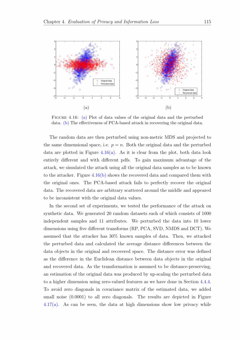
Chapter 4. Evaluation of Privacy and Information Loss 115
−3 −2 −1 0 1 2 3 4−4
−3
−2
−1
0
1
2
3
Original dataPerturbed data
(a)
−4 −3 −2 −1 0 1 2 3 4−4
−3
−2
−1
0
1
2
3
Original dataRecovered data
(b)
Figure 4.16: (a) Plot of data values of the original data and the perturbeddata. (b) The effectiveness of PCA-based attack in recovering the original data.
The random data are then perturbed using non-metric MDS and projected to
the same dimensional space, i.e. p = n. Both the original data and the perturbed
data are plotted in Figure 4.16(a). As it is clear from the plot, both data look
entirely different and with different pdfs. To gain maximum advantage of the
attack, we simulated the attack using all the original data samples as to be known
to the attacker. Figure 4.16(b) shows the recovered data and compared them with
the original ones. The PCA-based attack fails to perfectly recover the original
data. The recovered data are arbitrary scattered around the middle and appeared
to be inconsistent with the original data values.
In the second set of experiments, we tested the performance of the attack on
synthetic data. We generated 20 random datasets each of which consists of 1000
independent samples and 11 attributes. We perturbed the data into 10 lower
dimensions using five different transforms (RP, PCA, SVD, NMDS and DCT). We
assumed that the attacker has 30% known samples of data. Then, we attacked
the perturbed data and calculated the average distance differences between the
data objects in the original and recovered space. The distance error was defined
as the difference in the Euclidean distance between data objects in the original
and recovered data. As the transformation is assumed to be distance-preserving,
an estimation of the original data was produced by up-scaling the perturbed data
to a higher dimension using zero-valued features as we have done in Section 4.4.4.
To avoid zero diagonals in covariance matrix of the estimated data, we added
small noise (0.0001) to all zero diagonals. The results are depicted in Figure
4.17(a). As can be seen, the data at high dimensions show low privacy while

Chapter 4. Evaluation of Privacy and Information Loss 116
10987654322.1
2.2
2.3
2.4
2.5
2.6
2.7
2.8
2.9
3
Number of dimensions (p)
Avg.
Dis
tance
Err
or||x
−x||
RPPCASVDNMDSDCT
(a)
1009080706050403020102
2.05
2.1
2.15
2.2
2.25
2.3
2.35
2.4
Known Sample Size (%)
Avg.
Dis
tance
Err
or||x
−x||
RPPCASVDNMDSDCT
(b)
Figure 4.17: (a) Average distance error between the original and recovereddata at different dimensions. (b) The average distance error when using different
sizes of the known sample.
the data at low dimensions exhibit more resistance to the attack as the average
distance errors were high for all methods. This observation ensures that the data
at high dimensions typically represent the best fit of the original data where the
perturbation has a small effect on the structure of the covariance matrix. Both
NMDS and SVD approaches perform better and exhibit more resistance to the
attack than other methods. As expected, the SVD approach shows more privacy
due to the modification of some data entries below a predefined threshold. Indeed,
this is quite similar to the additive perturbation when a random noise is added to
the data. In contrast, the data transformed using PCA preserve a lower privacy
as the PCA subspace spanned by the principal directions of the perturbed data
maintains most proprieties of the PCA subspace of the known samples. The
performance of RP and DCT is quite similar at all dimensions.
To examine the effect of the size of known samples on the PCA-based attack,
we used 10 subsets of samples with different sizes (10%, 20%, . . . , 100%) from the
perturbed data at 5-dimensions. Note that the known samples do not need to
be subsets from the original data but they can also be any data that are drawn
from the same underlying distribution where the original data are drawn. For each
subset, we conducted the attack and reported the average distance error between
the recovered data and the original data. Figure 4.17(b) shows the results of this
experiment. Again, a clear win for both NMDS and SVD, particularly at high
dimensions. The known sample size seems to have a positive effect on the attack’s

Chapter 4. Evaluation of Privacy and Information Loss 117
success rate as the size increases the average distance error decreases.
We assess the performance of the attack on 15 real datasets taken from UCI
machine learning repository [58]. The description of all datasets is given earlier
in Table 4.2. As we exhaustively search for all PCs mirroring that guarantees
the best principle direction alignments (this requires to construct 2n matrices),
the computational cost of the attack goes up rapidly with the increase of the
number of dimensions. However, for data with modest number of dimensions,
the attack seems computationally efficient. To lighten this burden, we randomly
chose 10 dimensions for all datasets with more than 10 dimensions and attempted
to recover the original data. The average distance error between the original and
recovered data at different dimensions are plotted in Figure 4.18. All methods show
a similar performance on all datasets, but both NMDS and SVD maintain more
privacy than other methods where the recovered data are still on large distances
from the original ones. The worse performance was reported for PCA where the
error was lower than other methods at all dimensions. The results were rather
comparable for Iris, Ecoli and Handwritten Digits whereas for all other datasets
they were nearly close to each other. For some datasets (Breast Cancer Wisconsin,
Image Segementation and Handwritten Digits), the SVD outperforms the NMDS
and shows better privacy at all dimensions. The performance of the attack at
higher dimensions, i.e. p > 10, was approximately stable for all methods due to
the random choice of dimensions to represent the data. However, for the data at
lower dimensions, p <= 10, the error substantially increases whenever the number
of dimensions decreases.
We also measured data utility for all datasets in terms of information loss or
stress. The main objective of this is to get insight into which level the quality of
data utility can be lost in return for gaining a higher privacy for the perturbed data
produced by different transforms. As described earlier in Section 4.2, the stress
quantifies the average distortion in the pairwise distance. Figure 4.19 shows the
stress for all datasets at systematically reduced dimensions. Clearly, the NMDS
method substantially outperformed other methods in preserving distance at all
dimensions. From the results, plotted in Figures 4.18 and 4.19, it can be observed
that as p increases, all methods compromise privacy for better data utility, and
vice versa. This implies that increasing data utility by including large number of
dimensions may negatively affect the privacy of the perturbed data as the distance
error tends to be low compared with the error at lower dimensions. In this case,
the attacker may easily find a better recover of the original data. The growth

Chapter 4. Evaluation of Privacy and Information Loss 118
87654322.2
2.4
2.6
2.8
3
3.2
3.4
3.6
Number of dimensions (p)
Avg
.D
ista
nce
Err
or||x
−x||
Breast Cancer Wisconsin
RPPCASVDNMDSDCT
121110987654321.3
1.35
1.4
1.45
1.5
1.55
1.6
1.65
1.7
Number of dimensions (p)
Avg
.D
ista
nce
Err
or||x
−x||
Credit Approval
RPPCASVDNMDSDCT
322.35
2.4
2.45
2.5
2.55
2.6
Number of dimensions (p)
Avg
.D
ista
nce
Err
or||x
−x||
Iris
RPPCASVDNMDSDCT
21520017515012510075502510521.35
1.4
1.45
1.5
1.55
Number of dimensions (p)
Avg
.D
ista
nce
Err
or||x
−x||
Multiple Features
RPPCASVDNMDSDCT
181512107521.55
1.6
1.65
1.7
1.75
1.8
1.85
1.9
Number of dimensions (p)
Avg
.D
ista
nce
Err
or||x
−x||
Image Segementation
RPPCASVDNMDSDCT
5040302010522.44
2.46
2.48
2.5
2.52
2.54
2.56
2.58
2.6
2.62
2.64
Number of dimensions (p)
Avg
.D
ista
nce
Err
or||x
−x||
Spambase
RPPCASVDNMDSDCT
181512107522.58
2.6
2.62
2.64
2.66
2.68
2.7
2.72
2.74
2.76
Number of dimensions (p)
Avg
.D
ista
nce
Err
or||x
−x||
Hepatitis
RPPCASVDNMDSDCT
654322.5
2.55
2.6
2.65
2.7
2.75
2.8
2.85
2.9
Number of dimensions (p)
Avg
.D
ista
nce
Err
or||x
−x||
Ecoli
RPPCASVDNMDSDCT
121110987654321.4
1.5
1.6
1.7
1.8
1.9
2
Number of dimensions (p)
Avg
.D
ista
nce
Err
or||x
−x||
Wine
RPPCASVDNMDSDCT
63605040302010522.7
2.75
2.8
2.85
2.9
2.95
3
Number of dimensions (p)
Avg
.D
ista
nce
Err
or||x
−x||
Handwritten Digits
RPPCASVDNMDSDCT
765432
2.7
2.75
2.8
2.85
2.9
Number of dimensions (p)
Avg
.D
ista
nce
Err
or||x
−x||
Yeast
RPPCASVDNMDSDCT
353025201510521.56
1.58
1.6
1.62
1.64
1.66
1.68
1.7
1.72
Number of dimensions (p)
Avg
.D
ista
nce
Err
or||x
−x||
Satlog
RPPCASVDNMDSDCT
987654322.45
2.5
2.55
2.6
2.65
2.7
2.75
2.8
2.85
Number of dimensions (p)
Avg
.D
ista
nce
Err
or||x
−x||
Page Blocks
RPPCASVDNMDSDCT
5040302010522.35
2.4
2.45
2.5
Number of dimensions (p)
Avg
.D
ista
nce
Err
or||x
−x||
SCC
RPPCASVDNMDSDCT
7654322.55
2.6
2.65
2.7
2.75
2.8
Number of dimensions (p)
Avg
.D
ista
nce
Err
or||x
−x||
Pima−indian−diabets
RPPCASVDNMDSDCT
Figure 4.18: Average distance error between the original data, X, and therecovered data, X ′ at different dimensions using different perturbation methods.
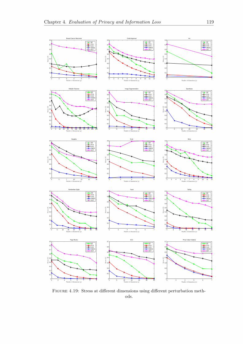
Chapter 4. Evaluation of Privacy and Information Loss 119
87654320
0.1
0.2
0.3
0.4
0.5
0.6
0.7
0.8
Number of dimensions (p)
Stre
ss(S
)
Breast Cancer Wisconsin
RPPCASVDNMDSDCT
121110987654320
0.1
0.2
0.3
0.4
0.5
0.6
0.7
0.8
Number of dimensions (p)
Stre
ss(S
)
Credit Approval
RPPCASVDNMDSDCT
320
0.1
0.2
0.3
0.4
0.5
0.6
0.7
0.8
Number of dimensions (p)
Stre
ss(S
)
Iris
RPPCASVDNMDSDCT
21520017515012510075502510520
0.1
0.2
0.3
0.4
0.5
0.6
0.7
0.8
0.9
1
Number of dimensions (p)
Stre
ss(S
)
Multiple Features
RPPCASVDNMDSDCT
181512107520
0.1
0.2
0.3
0.4
0.5
0.6
0.7
0.8
0.9
Number of dimensions (p)
Stre
ss(S
)
Image Segementation
RPPCASVDNMDSDCT
5040302010520
0.1
0.2
0.3
0.4
0.5
0.6
0.7
0.8
0.9
Number of dimensions (p)
Stre
ss(S
)
Spambase
RPPCASVDNMDSDCT
181512107520
0.1
0.2
0.3
0.4
0.5
0.6
0.7
0.8
Number of dimensions (p)
Stre
ss(S
)
Hepatitis
RPPCASVDNMDSDCT
654320
0.1
0.2
0.3
0.4
0.5
0.6
0.7
0.8
Number of dimensions (p)
Stre
ss(S
)
Ecoli
RPPCASVDNMDSDCT
121110987654320
0.1
0.2
0.3
0.4
0.5
0.6
0.7
0.8
Number of dimensions (p)
Stre
ss(S
)
Wine
RPPCASVDNMDSDCT
63605040302010520
0.1
0.2
0.3
0.4
0.5
0.6
0.7
0.8
0.9
Number of dimensions (p)
Stre
ss(S
)
Handwritten Digits
RPPCASVDNMDSDCT
7654320
0.1
0.2
0.3
0.4
0.5
0.6
0.7
Number of dimensions (p)
Stre
ss(S
)
Yeast
RPPCASVDNMDSDCT
353025201510520
0.1
0.2
0.3
0.4
0.5
0.6
0.7
0.8
0.9
Number of dimensions (p)
Stre
ss(S
)
Satlog
RPPCASVDNMDSDCT
987654320
0.1
0.2
0.3
0.4
0.5
0.6
0.7
0.8
0.9
Number of dimensions (p)
Stre
ss(S
)
Page Blocks
RPPCASVDNMDSDCT
5040302010520
0.1
0.2
0.3
0.4
0.5
0.6
0.7
Number of dimensions (p)
Stre
ss(S
)
SCC
RPPCASVDNMDSDCT
7654320
0.1
0.2
0.3
0.4
0.5
0.6
0.7
Number of dimensions (p)
Stre
ss(S
)
Pima−indian−diabets
RPPCASVDNMDSDCT
Figure 4.19: Stress at different dimensions using different perturbation meth-ods.

Chapter 4. Evaluation of Privacy and Information Loss 120
of dimension can be understood as injecting more data utility for the attack.
The consistency of sample eigenvectors with respect to the perturbed eigenvectors
would be achieved when the added dimensions have a little distortion in the ex-
isting structure of the covariance matrix. When the corresponding eigenvectors
derived from the covariance matrices for the known sample and the perturbed data
tend to be as far away from each other, it becomes difficult for the PCA-based
attack to match them correctly and thus high privacy can be achieved. To sum
up, the results show that NMDS is able to guarantee reasonable protection against
PCA-based attack and generate data with low information loss. The results also
suggest that the dimension in which the data are transformed into can certainly
reflect a trade-off between privacy and utility.
To quantify the influence of non-metric MDS perturbation on both the eigenval-
ues scale and the eigenvectors’ orientation of the covariance matrix of the known
sample with respect to the covariance matrix of the perturbed data, we used the
data produced by the five transforms at one reduced dimension, i.e. n − 1. For
each dataset, we compare the change in both the eigenvalues and the eigenvec-
tors where the size of known sample was varied from 10% to 100%. The changes
between the original and perturbed matrices were quantified using the two met-
rics, defined in (4.25) and (4.26)—the proportional change in the eigenvalues ratio
(shape) and the change in the direction of the eigenvectors (orientation).
Tables 4.3 and 4.4 show the average matching distance between the eigenvalues
and eigenvectors, respectively. The higher the value of the matching distance
the higher the privacy. The results indicate that both NMDS and SVD are both
dominant as the difference is higher than for the other methods. All other methods
(RP, PCA and DCT) perform quite similarly but the DCT performs slightly better
for most datasets. Again, the good performance of the SVD is more likely due to
the noise added to some entries in the lower dimensional data. This experiment
clearly shows that by using NMDS to perturb the original data we can discard a
large proportion of information embedded in the covariance matrix so that more
resistance against attacks that exploit the principal subspace can be provided.
Intuitively, as PCA attempts to minimise the least squares cost function, i.e. the
distance error of points to the PCs, it would be affected by the size of perturbation.
This means that if the data are projected on the subspace defined by any set
of the PCs that are obtained from the perturbed data, they may have different
PCs orientations, which cannot perfectly be aligned with the original PCs. We
conclude from these results that the more distortion the perturbation causes in

Chapter 4. Evaluation of Privacy and Information Loss 121
Table 4.3: Average change in eigenvalues’ scale using different sizes of theknown sample. The best result for each dataset is shown in bold.
Dataset RP PCA SVD NMDS DCT
Wine 0.3304 0.3162 0.4151 0.3156 0.3443BCW 0.2565 0.2674 0.2674 0.2683 0.2658Iris 0.4769 0.2246 0.8904 0.8249 0.7586Handwritten Digits 0.3511 0.3265 0.5082 0.5203 0.3586Ecoli 0.8074 0.7695 0.8874 0.8937 0.8819Image Segmentation 0.3045 0.2932 0.5122 0.4832 0.3475Multiple Features 0.5545 0.6212 0.6431 0.6643 0.6535Page Blocks 0.4337 0.7658 0.8523 0.7991 0.7877Spambase 0.7303 0.7483 0.8015 0.8089 0.7241Pima Diabetes 0.3900 0.4616 0.4315 0.4796 0.4686Yeast 0.6204 0.5840 0.5278 0.6809 0.6428Satlog 0.2734 0.2021 0.3271 0.4027 0.3349SCC 0.4760 0.3572 0.7787 0.6573 0.5559Credit Approval 0.7438 0.7362 0.8437 0.8539 0.7424Hepatitis 0.6685 0.6470 0.7906 0.7299 0.6597
Table 4.4: Average change in eigenvectors’ orientation using different sizes ofthe known sample. The best result for each dataset is shown in bold.
Dataset RP PCA SVD NMDS DCT
Wine 0.4719 0.7923 0.8482 0.7923 0.5717BCW 0.7130 0.7036 0.8337 0.8428 0.7353Iris 0.1269 0.4064 0.5143 0.4164 0.1836Handwritten Digits 0.1248 0.1043 0.2351 0.3106 0.1394Ecoli 0.4704 0.4125 0.4895 0.9106 0.4650Image Segmentation 0.1520 0.1264 0.2938 0.2429 0.1607Multiple Features 0.1034 0.0928 0.3856 0.4058 0.1487Page Blocks 0.5801 0.3305 0.9873 0.9305 0.3330Spambase 0.7060 0.8342 0.7907 0.9362 0.4867Pima Diabetes 0.3917 0.7695 0.7441 0.7884 0.1820Yeast 0.5438 0.6319 0.6679 0.9319 0.6530Satlog 0.1764 0.1507 0.6636 0.9503 0.2134SCC 0.1892 0.1618 0.3097 0.2618 0.2415Credit Approval 0.2756 0.4148 0.3179 0.4861 0.3787Hepatitis 0.8121 0.7825 0.8404 0.8084 0.7385
the covariance matrix the more difficult to match the principle components of the
perturbed data with their images in the original data.
To show the effect of the perturbation on the structure of the covariance matrix
for the original data, we perturbed 100 independent samples which are drawn from
a N(µ,Σ)-distribution with centre µ = (0, 0) and covariance matrix

Chapter 4. Evaluation of Privacy and Information Loss 122
−4 −3 −2 −1 0 1 2 3 4
−2
−1
0
1
2
3
4
← X
← 10 %← 20 %
← 30 %
(a) Rotation
−4 −3 −2 −1 0 1 2 3 4
−2
−1
0
1
2
3
4
5
← X
← 10 %
← 20 %
← 30 %
(b) RP
−4 −3 −2 −1 0 1 2 3 4
−2
−1
0
1
2
3
4
← X← 10 %
← 20 %← 30 %
(c) PCA
−2 −1 0 1 2 3 4−2
−1.5
−1
−0.5
0
0.5
1
1.5
2
2.5
3
← X
← 10 %← 20 %
← 30 %
(d) SVD
−5 0 5
−2
−1
0
1
2
3
4
5
← X
← 10 %
← 20 %
← 30 %
(e) NMDS
−3 −2 −1 0 1 2 3
−2.5
−2
−1.5
−1
−0.5
0
0.5
1
1.5
2
2.5
← X
← 10 %← 20 %
← 30 %
(f) DCT
Figure 4.20: Sample covariance matrix with 95% tolerance ellipses for theoriginal data, X. The 10%,20% and 30% ellipses represent the change in thecovariance matrix when 10%,20% and 30% samples, respectively, from the origi-nal data are replaced by their perturbed samples from the perturbed data using
different transforms (a)-(f).
Σ =
(0.69 1.25
1.25 3.25
).
We then perturbed the data using six different transforms. The estimated
tolerance ellipses based on the sample covariance matrix are visualised in Figure
4.20 for the original data as well as for modified data with different proportions of
independent perturbed samples. We replaced 10%,20% and 30% samples from the
original data by perturbed samples draw from the perturbed data, respectively.
The tolerance ellipses are constructed to cover exactly 95% of the data and they
are distinguished by different line styles. The centres of the ellipses are located at
the mean of the data. For NMDS, adding 10% perturbed samples slightly rotates
the tolerance ellipse based on the sample covariance matrix. The shape has also
been changed. The effects of 20% perturbed samples were in the same direction
and quite similar but a bit stronger. In the last case, 30% perturbed samples have a
large influence on the sample covariance matrix as the tolerance ellipse has started
to turn towards the perturbed samples. Furthermore, the sample mean has also
Chapter 4. Evaluation of Privacy and Information Loss 123
changed but still within the convex hull of the original data. For data rotation,
all three ellipses seem quite similar and almost coincide with each other retaining
the shape and the orientation of the covariance matrix. This is due to the fact
that data rotation exactly preserves distance as well as the geometric shape, i.e.
it changes the directions of vectors, but leaves their magnitude unchanged. The
RP and PCA show quite similar performance, their impact was relatively low. For
both SVD and DCT, the variation of the perturbation influence was small where
all ellipses closely follow the same shape of the original ellipse. Interestingly, the
sample mean approximately remains unchanged along all the replacements.
We observe that depending on the size of perturbation, the covariance ellipse
strongly changes its orientation (the correlation between variables is affected) and
its shape (variation). Generally speaking, the perturbed samples would be seen as
outliers that tend to rotate the PCs axes towards them and change the correlation
structure of the data. Therefore, it would be more difficult for a PCA-based
attack to successfully align the principle components for the known samples with
the principle components for the perturbed data.
What we can conclude from the above results is that non-metric MDS heavily
distorts the structure of covariance matrix and thus high privacy protection is
achieved. However, as we will see in Chapter 5, non-metric MDS maintains much
distance-related properties as the accuracy when data mining algorithm operates
on the perturbed data is similar (if not better) to the accuracy obtained from the
original data. Furthermore, when we apply the PCA-based attack on the per-
turbed data which are represented in non-isometric space, the eigenvalues derived
from the sample data are not the same as those derived from the perturbed data.
Hence, we cannot derive any transformation basis that can be used to reverse the
non-metric MDS transformation back and thus disclose the original data. In other
words, PCA-based attack would not work any more.
4.6 Summary
In this chapter, we have discussed the concept of data utility in the context of
distance-based data mining and defined a measure that can express the amount
of information lost as a result of transforming data into lower dimensions. We
also analysed two types of inference attacks that would threat our perturbation
technique and jointly evaluated them with data utility.

Chapter 4. Evaluation of Privacy and Information Loss 124
In the first attack (distance-based attack), we considered a scenario in which the
data owner releases the data such that the distances between objects are exactly
preserved and the attacker has prior knowledge about some data points and their
distances to an attacked point. The disclosure would occur with high probability
when the attacker attempts to find a best fit mapping between these points and
their images in the perturbed data using some heuristic methods. Here, we noticed
that the data in high dimensions can preserve better privacy and utility. When the
data are transformed into a few lower dimensions from the original dimensionality,
they often preserve the pairwise distance, demonstrating good utility for distance-
based analysis. However, as non-metric MDS utilises the rank order of the distance
not their magnitude, the points are located within uncertain areas which may
hinder the distance-based attack from determining the exact location of the points.
In the second attack (PCA-based attack), we assumed that the attacker either
has a subset of the original data samples or knows the distribution from where the
original data was drawn. Then the attacker can exploit the characteristics of the
covariance matrices of both the perturbed data and the known sample to estimate
the original data values. Roughly speaking, when the transformation basis does
not change the shape of distributions, i.e. the eigenspace derived from the sample
data is close to that derived from the transformed data, the transformation basis
can be easily identified and hence the original data can be recovered. For this kind
of attack, the preservation of privacy and utility is merely a trade-off.
The experiments show that the perturbed data, produced by non-metric MDS,
demonstrate good resilience to the two above attacks compared with some other
well-known transforms. We conclude that non-metric MDS is a good competi-
tive perturbation technique as it can effectively hide information and limit the
disclosure sufficiently.

Chapter 5
Evaluation of Distance-Based
Clustering and Classification
Data clustering and classification are two of the challenging distance-based mining
tasks exploited in the KDD process. Clustering analysis is the task of segmenting
a database, containing a set of objects, into subsets or groups called clusters. The
notion of clusters can be described in many ways including groups, where instances
in the same group more closely match each other than instances in different groups,
dense areas of the data space or particular statistical distributions. Classification
is a low level data mining task that assigns a set of objects in a given dataset
to target categories or classes. The main goal of classification is to accurately
predict the target class for each case in the data. For example, in retail industry,
a classification model could be used to identify customer loyalty as high loyalty,
satisfied, or low loyalty. In general, the most popular practice of clustering and
classification requires a measure of “distance” or “closeness”.
The structure of this chapter is as follows. Section 5.1 briefly introduces
distance-based clustering and classification in PPDM. Section 5.2 precisely de-
fines the data mining task of clustering and evaluates the utility and privacy of
the perturbed data for clustering analysis. Section 5.3 introduces the concept of
distance-based classification and discusses the utility and privacy of the perturbed
data in the context of data classification. Each section has a set of experiments and
results that evaluates the effectiveness of non-metric MDS and compares it with
some other well-known methods. Finally, Section 5.4 presents a brief summary of
the whole chapter.
125

Chapter 5. Evaluation of Distance-Based Clustering and Classification 126
5.1 Introduction
Clustering aims to find suitable partitions in huge amounts of data without any
supervision, guidance or prior knowledge. It attempts to maximise the similarity
of objects belonging to the same cluster and minimise the similarity of objects in
different clusters. As described in Section 2.3.4, many different clustering methods
have been proposed in order to solve this problem from different perspectives,
i.e. partition-based clustering, density-based clustering, hierarchical clustering
and grid-based methods. In general, most of these methods utilises a distance
function to define the relationship between data objects. That is, the cluster is
defined and formed when it satisfies a certain distance criterion.
On the other hand, classification algorithms typically find relationships between
the values of the predictors and the values of the target during the training phase.
The classification task begins with a set of data objects in which the class as-
signments are known a priori and attempts to build a model, which can then be
applied to unseen data cases in which the class assignments are unknown. For
example, a classification model that predicts risk of infection of a disease could be
developed based on observed data for many patients over a period of time. The
medical history might involve a set of variables including blood pressure, family
history, location, age, and so on. Infection risk would be the target, the other
variables would be the predictors, and the data for each patient would constitute
a case. This is a simplest type of classification problem where the target attribute
has only two possible values, e.g. high risk or low risk. Multi-class targets have
more than two values, e.g. low, medium, high, or unknown. Note that most
distance-based classification algorithms, e.g. k-NN and SVM, are known as lazy
learners [160]. These algorithms often predict the class of the new objects directly
from the training instances without having to maintain a model derived from the
data.
As long as the analysis utilises the distance generating a configuration of points
at any lower dimension in which the pairwise distances are well preserved would
be sufficient to maintain high data utility. Note that there is no perfect mapping
preserving all of the data properties at the same time, rather each mapping is a
compromise best suited for a particular analysis purpose. The projection of data
into a lower space often results in some data distortion; and as we are interested in
discovering groups within the data, this distortion should be minimised to guaran-
tee the quality of the analysis. The lower the distortion, the lower the information

Chapter 5. Evaluation of Distance-Based Clustering and Classification 127
loss and the higher the utility of the perturbed data. However, to ensure the
preservation of privacy, the increases of utility should not lead to disclosing the
original data. We want to minimise the disclosure risk as much as possible so that
better privacy of the perturbed data can be achieved.
In this chapter, we investigate the usability of distance-based clustering and
classification algorithms on the perturbed data that are generated using non-metric
MDS and compare it with some other dimensionality reduction techniques used
for PPDM, including RP, PCA, SVD and DCT. We hypothesise that non-metric
MDS is a good competitive tool for PPDM. The quality of the perturbed data
has been evaluated from the perspectives of model accuracy and disclosure risk.
More specifically, we evaluate the utility of the perturbed data in clustering and
classification analysis using a variety of distance-based algorithms and measure
how good the results obtained from the perturbed data are compared with the
results obtained from the original data. In addition, we consider the same set of
attacks proposed in Chapter 4 in order to examine the privacy associated with per-
turbed data using different dimensionality reduction techniques and evaluate the
trade-off between privacy and accuracy of distance-based algorithms. We compare
these techniques on a number of benchmark datasets and test the performance at
different number of dimensions to show how this would affect the analysis.
5.2 Application to Clustering Tasks
5.2.1 The Task of Distance-Based Clustering
In this section, we precisely define the task of clustering and explore a number of
distance-based clustering algorithms. This may help us to assess the suitability and
usefulness of the perturbed data generated by non-metric MDS for distance-based
analysis. Clustering is the process of recognising natural groupings or clusters
in data based on some similarity measures [82]. The similarity between any pair
of objects can be evaluated using any of the distance metrics defined in Section
2.3.1. In general, the problem of clustering is described as follows: given m objects,
allocate each object to one of k clusters and minimise the sum of squared Euclidean
distances between each object and the centroid or representative object of the
cluster.
Partitional clustering attempts to optimise a certain criterion function in order
to find a number of partitions in the data. For instance, the most commonly
Chapter 5. Evaluation of Distance-Based Clustering and Classification 128
used algorithm (k-means) aims to minimise the distance of each object from the
centre of the cluster containing that object. The objective function, i.e. the sum
of squared error (SSE) is described by
SSE =k∑i=1
∑x∈Ci
||ci − x||2, (5.1)
where ci is the centroid (mean) of the ith cluster, Ci, while ||ci−x|| is the Euclidean
distance between an object x and ci. The centroid ci is defined by
ci =1
mi
∑x∈Ci
x, (5.2)
where mi is the number of objects in Ci. That is, the best centroid for minimising
the SSE of a cluster is the mean of objects in the cluster [160]. Let ck be the kth
centroid, the differentiation of Equation (5.1) can minimises the SSE, i.e.
∂
∂ckSSE =
∂
∂ck
k∑i=1
∑x∈Ci
||ci − x||2
=k∑i=1
∑x∈Ci
∂
∂ck||ci − x||2
=∑x∈Ck
2 ||ck − xk|| = 0
∑x∈Ck
2 ||ck − xk|| = 0⇒ ck =1
mk
∑x∈Ck
xk. (5.3)
Hierarchical clustering is another method to analyse grouping in the data over
a variety of scales of distance by creating a tree-like graph. The data objects
are connected to each other to form clusters based on their distance. Apart from
the normal choice of distance functions, one also needs to decide on the linkage
criterion. Popular choices are known as single linkage (the minimum distance
between two objects in different clusters), complete linkage (the maximum distance
between two objects in different clusters) or average linkage (the average distance
of all pair of objects from different clusters). Techniques for hierarchical clustering
generally fall into two types—agglomerative and divisive. In this chapter, we
consider an agglomerative technique [74] where the tree is a multi-level hierarchy
and clusters at one level are merged into clusters at the next higher level. If the

Chapter 5. Evaluation of Distance-Based Clustering and Classification 129
proximities are distances, then the shortest edge between two nodes in different
subset of nodes is one way to define cluster closeness and decide if any two clusters
should be combined or not. The cluster proximity G(Ci, Cj) of cluster Ci and
cluster Cj can be defined by
G(Ci, Cj) = min{||x− y||} for all x ∈ Ci and y ∈ Cj. (5.4)
Density-based clustering locates regions of high density of objects in the data
that are separated from one another regions of low density. DBSCAN [55] is an
example of a simple and effective density-based clustering algorithm that estimates
the density of a given point by counting its kth nearest neighbour points within
a specified radius, r. The neighbourhood of a given point, c, can be defined as a
closed region, A, in the space such that a point, x, is in the region A if and only
if ||x− c|| ≤ r where c is located at the centre of the circle of radius r.
5.2.2 Cluster Validity Evaluation
To evaluate the effectiveness of our proposed perturbation method, we compared
the quality of the generated clusters on both the original data, X, and the per-
turbed data, Y . Intuitively, when the clustering results from Y are the same, or
very nearly the same, as those obtained from X, we can say that Y are analytically
as useful for clustering analysis as X.
Given two datasets, X and Y , with n objects. Assume that we have a parti-
tion C = {C1, C2, . . . , Ck}, from X, and C ′ = {C ′1, C ′2, . . . , C ′k}, from Y , where
∪ki=1Ci = X, ∪ki=1C′i = Y and Ci ∩ Cj = ∅, C ′i ∩ C ′j = ∅ for all 1 ≤ i 6= j ≤ k,
where k is the number of clusters. Many various clustering validation were used to
evaluate the performance of clustering algorithms [70], all of which have different
properties and it remains unknown in practice which the most suitable measure
to use. Due to the desirable theoretical properties that make it a true metric,
we use variation of information (V I) [116] as a relative clustering validation tool.
The V I is based on information theory and measures the amount of information
that is gained or lost in changing from one clustering to another. A low value of
V I infers that the two clusterings, C and C ′ are quite similar, while a high value
infers the opposite. To compare the results and show how C and C ′ are related,
we first construct a contingency table (Table 5.1) that tabulates the results of C
against the results of C ′.
Then we calculate V I using

Chapter 5. Evaluation of Distance-Based Clustering and Classification 130
Table 5.1: A contingency table: Clustering C × C ′
C ′1 C ′2 . . . . . . C ′k∑
C1 n11 n12 . . . . . . n1k n1.
C2 n21 n22 . . . . . . n2k n2.
......
... . . . . . . ......
Ck nk1 nk2 . . . . . . nkk nk.∑n.1 n.2 . . . . . . n.k n
V I = H(C) +H(C ′)− 2MI(C,C ′), (5.5)
where H(C) and H(C ′) are the entropy of clusterings C and C ′, respectively,
and MI(C,C ′) is the mutual information between C and C ′. The entropy of a
clustering Ci with a probability function p(Ci) is defined by
H(Ci) = −k∑i=1
p(Ci) log2 p(Ci). (5.6)
The mutual information, MI(C,C ′), gives how much the knowledge of C ′ can
reduce the uncertainty of C [39]. In other words, the mutual information measures
the dependency between C and C ′. It is always non-negative and is equal to zero,
if and only if C and C ′ are independent, i.e. C ∩C ′ = ∅. The mutual information,
MI(C,C ′) of clustering C and C ′ is defined as
MI(C,C ′) = H(C)−H(C|C ′) =k∑
C,C′
p(C,C ′) log2
p(C,C ′)
p(C)p(C ′), (5.7)
where p(C,C ′) is the joint probability function of C and C ′.
By using the contingency table, the equation (5.5) can be rewritten as follows:
V I = −k∑i=1
ni.n
log2
ni.n−
k∑j=1
n.jn
log2
n.jn− 2
k∑i=1
k∑j=1
nijn
log2
(nij/n)
(ni.
n)(n.j
n), (5.8)
where n is the total number of records, k is the number of clusters, ni./n and n.j/n
are the marginal probabilities of clustering Ci and clustering C ′j, respectively, and
nij/n is the joint probability that a record belongs to both Ci and C ′j. Note that

Chapter 5. Evaluation of Distance-Based Clustering and Classification 131
the V I metric is bounded by 2 log k.
5.2.3 Experiments and Results
In this section, we present three sets of experiments on evaluating the effectiveness
of the proposed method (NMDS) and compare it with the four other perturba-
tion techniques (RP, PCA, SVD and DCT). The first set of experiments (Section
5.2.3.2) evaluates the quality of the obtained clusterings from the original and per-
turbed data and measures the similarity between the two clusterings. The second
set of experiments (Section 5.2.3.3) tests and analyses whether the clusters are sig-
nificantly different before/after the perturbation and whether there are significant
differences in the performance of all the five techniques. The third set of experi-
ments (Section 5.2.3.4) studies the relationship between the privacy and accuracy
of the perturbed data at different dimensions and compares the performance across
all techniques.
5.2.3.1 Datasets and Experimental Setup
The work in this chapter is motivated by real world problems where obtaining ac-
curate clustering results depends on how much utility is preserved in the perturbed
data. We attempt to examine this feature in the perturbed data using three dif-
ferent clustering methods, i.e. partition-based clustering, hierarchical clustering
and density-based clustering. Meanwhile, we evaluate the trade-off between the
privacy and utility for the perturbed data at different number of dimensions. In
our experiments, we considered the same 15 datasets used in Section 4.4.4. A brief
description of all datasets is represented in Table 5.2 after including the number of
real classes for each dataset. A detailed description of each dataset can be found
in [58].
All datasets are ideal for clustering and classification analysis when the task is
to assign each object to its proper cluster or class. Each dataset is represented
as an m × n matrix where each row corresponds to an object and each column
represents a variable. We cleansed the data to eliminate the effect of missing values
on the distance measure as follows: if the number of records that have one or more
missing values is 2% or less of the total size of the data, we removed these records
from the dataset. Otherwise, we replaced the entries of missing values with zeros.
Although this simple method may be problematic in terms of data quality [160],

Chapter 5. Evaluation of Distance-Based Clustering and Classification 132
Table 5.2: A description of datasets used in our experiments.
Dataset m n Classes
Iris 150 4 3Wine 178 13 3Breast Cancer Wisconsin (BCW) 699 9 2Handwritten Digits 3823 64 10Ecoli 336 7 8Image Segementation 2100 19 7Multiple Features 2000 216 10Page Blocks 5473 10 5Spambase 4601 57 2Pima-indian-diabets 768 8 2Yeast 1484 8 10Satlog 2000 36 6Hepatitis 155 19 2Synthetic Control Chart (SCC) 600 60 6Credit Approval 690 14 2
our concern at this stage is rather to mitigate the effect of missing values and
facilitate the task of the distance-based algorithms
In our experiments, we used MATLAB implementations to perturb and cluster
the data. The perturbation processes were carried out as follows: we normalized
the original data, X, so all variables had zero mean and σ = 1. This helped
in preventing one variable dominating the others in terms of Euclidean distance.
Then, the dissimilarities, δij, between the records in X were calculated using
(3.6). Then, we transformed the dissimilarities and generated the perturbed data,
Y , in p-dimensional space as illustrated previously. We then used the generated
data, Y , to carry out the clustering analysis and compare it with results obtained
from X. The initial configuration was determined by choosing the p non-negative
eigenvalues of the dissimilarities matrix ∆. However, to avoid accepting this initial
configuration as a final solution of non-metric MDS, we used a random initial
configuration for all data that have the best stress at its initial configuration.
This has been discussed in Section 3.3.2. To show how much information is lost as
a result of the transformation, we computed the deviation of the pairwise distances
in the original and perturbed spaces which has been quantified by using the stress
(4.3).
To obtain as fair as possible comparison, the dimensionality of the data, p, was
systematically reduced to the same lower dimensions for all perturbation tech-
niques. That is, for NMDS, the number of dimensions was manually adjusted to

Chapter 5. Evaluation of Distance-Based Clustering and Classification 133
produce data in p-dimensional space. For RP, we used a random projection matrix
of p columns. For PCA and SVD, we chose the first p components. For DCT, we
chose the p dimensions corresponding to the highest p frequencies of high energy
coefficients.
The experimental parameters for clustering were set up as follows. For each
dataset, the number of clusters k was set as the number of classes. To guarantee
stable clustering results, we determined the mean of the true classes as initial
centroids for the k-means algorithm both for the original and perturbed data.
In k-means, the initial seeds (centroids) are chosen randomly and thus the final
clustering can vary with each run due to this initial selection. Our deterministic
allocation of initial cluster centroids allows us to measure how the clusters obtained
from both data (X and Y ) compare without having to account for the randomness
of the k-means algorithm. DBSCAN is very sensitive to both the radius, r, of
the neighbourhood and the minimum number of points in the neighbourhood,
k. Points in a cluster Ci often have k nearest neighbours at roughly the same
distances, whereas noise points have k nearest neighbours at farther distances.
For this set of experiments, we have set k = 4. We compute the distances of
k nearest neighbours for all data points and sort them in ascending order. The
distances are then plotted to see at which point there is a sharp change. That is,
the value of distance at this point would be quite suitable for the radius, r.
To assess whether or not the clusters obtained from the perturbed data are
significantly different from the clusters obtained from the original data, we used
paired t-test [46] on the V I scores that are derived from 30 independent samples
of comparing the clusterings on the original and perturbed data. Additionally, we
also used paired t-test to examine whether or not NMDS is achieved a statistically
significant improvement over the other perturbation methods.
5.2.3.2 Comparison of Clusterings
This section presents experimental evaluation of the proposed technique in terms of
clustering accuracy and compares it with some existing methods, which are stated
earlier. Our hypothesis is that the clusters obtained from the perturbed data, Y ,
should be similar to those obtained from the original data, X. The purpose of this
comparison is not to determine which is the best clustering algorithm, but rather
to assess the performance of the algorithms on the perturbed data generated using
different perturbation methods.

Chapter 5. Evaluation of Distance-Based Clustering and Classification 134
We compared the accuracies of k-means, hierarchical clustering and DBSCAN
on the original and perturbed data using the variation of information (V I) measure
(5.5). We assessed the amount of utility that would be required in order to obtain
good clustering results at given dimensionality. We decreased the number of di-
mensions to see how this would affect data utility and to find an acceptable value
of p by repeating the analysis using different values of p. Our initial observations
were that when the data in the higher n-dimensional space are transformed into
a lower p-dimensional space, p > n/2, the generated clustering results obtained
from Y are almost the same as those obtained from X, with 0 ≤ V I < (2 log k)/2.
For instance, for the Wine dataset, we obtained a very low value of variation of
information (V I < 0.08) using k-means, for all Y with p = 5, . . . , 12, but the value
of V I increased for k < 5. A similar behaviour can be observed when hierarchical
clustering and DBSCAN are used, but with p = 7 as a cut-off point. This obser-
vation confirms that the best trade-off between information loss and accuracy can
be easily determined at the point when the value of the stress starts to increase
sharply, i.e. at the elbow of the S curve.
Figure 5.1, 5.2 and 5.3 show a comparison of the clustering variation between
X and Y using k-means, hierarchical clustering and DBSCAN, respectively, at
different p dimensions. We note that the clustering results on Y that are produced
using PCA and NMDS are very similar. However, for most datasets, NMDS
preserves much of data utility even at very low dimensions. RP and SVD lead to
poor clustering results because the values of VI were high compared with PCA
and NMDS. The results of DCT remain on average higher than those of all other
methods, indicating low data utility. For some datasets, RP has a high variation
of V I when changing from one dimensional space to another which is more likely
due the randomness of choosing the projection matrix. On the other hand, the
performance of DCT was relatively stable at all dimensions for the three clustering
techniques. This implies that no advantage is gained using DCT, and the size of
distortion caused by this method does not depend on the number of selected
dimensions.
The results shown in the above figures demonstrate the good performance of
NMDS in comparison to other dimensionality reduction methods. The obtained
clusters from Y using NMDS were almost identical to those from X as the values of
V I were low for most dataset and for the three clustering techniques, particularly
at high dimensions. The clustering results for PCA, using both k-means and
hierarchical clustering, were similar to NMDS, displaying low V I. However, for

Chapter 5. Evaluation of Distance-Based Clustering and Classification 135
87654320
0.2
0.4
0.6
0.8
1
1.2
1.4
1.6
1.8
2
Number of dimensions (p)
VI
Breast Cancer Wisconsin
RPPCASVDNMDSDCT
121110987654320
0.2
0.4
0.6
0.8
1
1.2
1.4
Number of dimensions (p)
VI
Credit Approval
RPPCASVDNMDSDCT
320
0.5
1
1.5
2
2.5
3
Number of dimensions (p)
VI
Iris
RPPCASVDNMDSDCT
2152001751501251007550251050
1
2
3
4
5
6
7
Number of dimensions (p)
VI
Multiple Features
RPPCASVDNMDSDCT
181512107520
1
2
3
4
5
6
Number of dimensions (p)
VI
Image Segementation
RPPCASVDNMDSDCT
5040302010520
0.2
0.4
0.6
0.8
1
1.2
1.4
Number of dimensions (p)
VI
Spambase
RPPCASVDNMDSDCT
181512107520
0.1
0.2
0.3
0.4
0.5
0.6
0.7
0.8
Number of dimensions (p)
VI
Hepatitis
RPPCASVDNMDSDCT
654320
1
2
3
4
5
6
Number of dimensions (p)
VI
Ecoli
RPPCASVDNMDSDCT
121110987654320
0.5
1
1.5
2
2.5
3
3.5
Number of dimensions (p)
VI
Wine
RPPCASVDNMDSDCT
63605040302010520
1
2
3
4
5
6
7
Number of dimensions (p)
VI
Handwritten Digits
RPPCASVDNMDSDCT
7654320
1
2
3
4
5
6
7
Number of dimensions (p)
VI
Yeast
RPPCASVDNMDSDCT
353025201510520
0.5
1
1.5
2
2.5
3
3.5
4
4.5
5
Number of dimensions (p)
VI
Satlog
RPPCASVDNMDSDCT
987654320
0.1
0.2
0.3
0.4
0.5
0.6
0.7
0.8
0.9
1
Number of dimensions (p)
VI
Page Blocks
RPPCASVDNMDSDCT
5040302010520
0.5
1
1.5
2
2.5
3
Number of dimensions (p)
VI
SCC
RPPCASVDNMDSDCT
7654321
1.1
1.2
1.3
1.4
1.5
1.6
1.7
1.8
1.9
2
Number of dimensions (p)
VI
Pima−indian−diabets
RPPCASVDNMDSDCT
Figure 5.1: The variation of information (V I) of RP, PCA, SVD, NMDS andDCT using k-means.

Chapter 5. Evaluation of Distance-Based Clustering and Classification 136
87654320
0.02
0.04
0.06
0.08
0.1
0.12
Number of dimensions (p)
VI
Breast Cancer Wisconsin
RPPCASVDNMDSDCT
121110987654320
0.05
0.1
0.15
0.2
0.25
0.3
0.35
Number of dimensions (p)
VI
Credit Approval
RPPCASVDNMDSDCT
320
0.5
1
1.5
2
2.5
3
Number of dimensions (p)
VI
Iris
RPPCASVDNMDSDCT
2152001751501251007550251050
0.02
0.04
0.06
0.08
0.1
0.12
0.14
0.16
Number of dimensions (p)
VI
Multiple Features
RPPCASVDNMDSDCT
18151210752−0.1
0
0.1
0.2
0.3
0.4
0.5
0.6
0.7
0.8
Number of dimensions (p)
VI
Image Segementation
RPPCASVDNMDSDCT
5040302010520
0.05
0.1
0.15
0.2
0.25
0.3
0.35
Number of dimensions (p)
VI
Spambase
RPPCASVDNMDSDCT
181512107520.05
0.1
0.15
0.2
0.25
0.3
0.35
0.4
0.45
Number of dimensions (p)
VI
Hepatitis
RPPCASVDNMDSDCT
654320
0.2
0.4
0.6
0.8
1
1.2
1.4
Number of dimensions (p)
VI
Ecoli
RPPCASVDNMDSDCT
12111098765432−0.05
0
0.05
0.1
0.15
0.2
0.25
0.3
0.35
0.4
Number of dimensions (p)
VI
Wine
RPPCASVDNMDSDCT
63605040302010520
0.01
0.02
0.03
0.04
0.05
0.06
0.07
0.08
0.09
0.1
Number of dimensions (p)
VI
Handwritten Digits
RPPCASVDNMDSDCT
7654320.05
0.1
0.15
0.2
0.25
0.3
0.35
0.4
Number of dimensions (p)
VI
Yeast
RPPCASVDNMDSDCT
353025201510520
0.1
0.2
0.3
0.4
0.5
0.6
0.7
Number of dimensions (p)
VI
Satlog
RPPCASVDNMDSDCT
987654320
0.02
0.04
0.06
0.08
0.1
0.12
Number of dimensions (p)
VI
Page Blocks
RPPCASVDNMDSDCT
5040302010520.5
1
1.5
2
2.5
3
Number of dimensions (p)
VI
SCC
RPPCASVDNMDSDCT
7654320
0.01
0.02
0.03
0.04
0.05
0.06
0.07
0.08
0.09
Number of dimensions (p)
VI
Pima−indian−diabets
RPPCASVDNMDSDCT
Figure 5.2: The variation of information (V I) of RP, PCA, SVD, NMDS andDCT using hierarchical clustering.

Chapter 5. Evaluation of Distance-Based Clustering and Classification 137
87654320.4
0.6
0.8
1
1.2
1.4
1.6
1.8
2
2.2
2.4
Number of dimensions (p)
VI
Breast Cancer Wisconsin
RPPCASVDNMDSDCT
121110987654320.4
0.6
0.8
1
1.2
1.4
1.6
1.8
2
Number of dimensions (p)
VI
Credit Approval
RPPCASVDNMDSDCT
320
0.5
1
1.5
2
2.5
Number of dimensions (p)
VI
Iris
RPPCASVDNMDSDCT
2152001751501251007550251050
0.2
0.4
0.6
0.8
1
1.2
1.4
1.6
1.8
Number of dimensions (p)
VI
Multiple Features
RPPCASVDNMDSDCT
181512107520
0.5
1
1.5
2
2.5
3
3.5
4
4.5
Number of dimensions (p)
VI
Image Segementation
RPPCASVDNMDSDCT
5040302010520
0.1
0.2
0.3
0.4
0.5
0.6
0.7
0.8
0.9
1
Number of dimensions (p)
VI
Spambase
RPPCASVDNMDSDCT
181512107520.4
0.6
0.8
1
1.2
1.4
1.6
1.8
Number of dimensions (p)
VI
Hepatitis
RPPCASVDNMDSDCT
654320
0.5
1
1.5
2
2.5
Number of dimensions (p)
VI
Ecoli
RPPCASVDNMDSDCT
121110987654320
0.1
0.2
0.3
0.4
0.5
0.6
0.7
0.8
0.9
Number of dimensions (p)
VI
Wine
RPPCASVDNMDSDCT
63605040302010520
0.1
0.2
0.3
0.4
0.5
0.6
0.7
0.8
Number of dimensions (p)
VI
Handwritten Digits
RPPCASVDNMDSDCT
7654320.2
0.25
0.3
0.35
0.4
0.45
0.5
0.55
0.6
0.65
Number of dimensions (p)
VI
Yeast
RPPCASVDNMDSDCT
353025201510520
0.5
1
1.5
2
2.5
Number of dimensions (p)
VI
Satlog
RPPCASVDNMDSDCT
987654320
0.1
0.2
0.3
0.4
0.5
0.6
0.7
0.8
0.9
1
Number of dimensions (p)
VI
Page Blocks
RPPCASVDNMDSDCT
5040302010520
0.2
0.4
0.6
0.8
1
1.2
1.4
Number of dimensions (p)
VI
SCC
RPPCASVDNMDSDCT
765432
0.4
0.5
0.6
0.7
0.8
0.9
1
1.1
1.2
1.3
Number of dimensions (p)
VI
Pima−indian−diabets
RPPCASVDNMDSDCT
Figure 5.3: The variation of information (V I) of RP, PCA, SVD, NMDS andDCT using DBSCAN.

Chapter 5. Evaluation of Distance-Based Clustering and Classification 138
RP, SVD and DCT, the clustering results for those techniques showed higher values
of V I, indicating lower data utility. The results of V I for hierarchical clustering
were very low compared with k-means and DBSCAN, but that may be because
hierarchical clustering generates only a low number of clusters and thus it assigns
many objects to a single group. This leads to low variation of clusterings on X
and Y . For DBSCAN, NMDS outperforms other methods exhibiting high data
utility for clustering.
Moreover, the results suggest that transforming the original data into the few
lower dimensions from the original dimensionality is sufficient to maintain most of
the distance-related properties. This can be concluded from the low values of V I
at high dimensions. This is not surprising, since if the distance is well preserved
in the lower dimensional space, it would rather be easier for any distance-based
algorithm to discover the real clusters underlying the data. When the utility is
most important for the data owner, the best strategy is to retain as much as
features in the perturbed data.
5.2.3.3 Statistical Significance Testing
In this section, we evaluate the difference in the performance of the clustering
on the original and perturbed data using different transforms (RP, PCA, SVD,
NMDS and DCT). We hypothesis that clusters produced on the original data are
not significantly different to those on the perturbed data. For a fair comparison,
we transformed the original data into a fixed number of dimensions, i.e. one
reduced dimension, which often gives a good representation of the original data.
To test the performance when changing the clustering from the original data to
the perturbed data, we calculated the average differences of clustering membership
for objects before and after the perturbation, i.e. the average difference of the
validation measure (V I). We conducted 30 trials of k-means on both the original
and perturbed data and measure the correlation of the obtained clusters with
respect to the true classes using V I. We then estimated the variance of the mean
difference of V I using paired t-test [46] at 95% confidence level.
Tables 5.3 show the observed p-values of all methods. The values less than %5
are sufficient evidence to reject the null hypothesis, which is: no difference exists
between the means of V I scores before and after the perturbation. The results
reveal that both PCA and NMDS show better performance over others methods
for most datasets and indicate the consistency of the clustering when changing
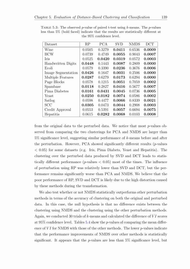
Chapter 5. Evaluation of Distance-Based Clustering and Classification 139
Table 5.3: The observed p-value of paired t-test using k-means. The p-valuesless than 5% (bold faced) indicate that the results are statistically different at
the 95% confidence level.
Dataset RP PCA SVD NMDS DCT
Wine 0.0505 0.3279 0.0411 0.6536 0.0009BCW 0.0739 0.4749 0.0055 0.9043 0.0007Iris 0.0525 0.0420 0.0319 0.0572 0.0003Handwritten Digits 0.0448 0.1443 0.0087 0.2809 0.0000Ecoli 0.0579 0.3390 0.0236 0.3676 0.0006Image Segmentation 0.0426 0.1647 0.0031 0.2506 0.0000Multiple Features 0.0287 0.6279 0.0173 0.6294 0.0000Page Blocks 0.0578 0.1215 0.0051 0.7059 0.0002Spambase 0.0118 0.2827 0.0416 0.5677 0.0007Pima Diabetes 0.0161 0.0431 0.0045 0.0736 0.0005Yeast 0.0250 0.0182 0.0074 0.0586 0.0002Satlog 0.0598 0.4477 0.0066 0.8339 0.0021SCC 0.0305 0.0473 0.0044 0.2908 0.0003Credit Approval 0.0553 0.5391 0.0057 0.6694 0.0075Hepatitis 0.0615 0.0282 0.0068 0.0103 0.0008
from the original data to the perturbed data. We notice that most p-values ob-
served from comparing the two clusterings for PCA and NMDS are larger than
5% significance level, suggesting similar performance of k-means before and after
the perturbation. However, PCA showed significantly different results (p-values
< 0.05) for some datasets (e.g. Iris, Pima Diabets, Yeast and Hepatitis). The
clustering over the perturbed data produced by SVD and DCT leads to statis-
tically different performance (p-values < 0.05) most of the times. The influence
of perturbation using RP was relatively lower than SVD and DCT, but the per-
formance remains significantly worse than PCA and NMDS. We believe that the
poor performance of RP, SVD and DCT is likely due to the high distortion caused
by these methods during the transformation.
We also test whether or not NMDS statistically outperforms other perturbation
methods in terms of the accuracy of clustering on both the original and perturbed
data. In this case, the null hypothesis is that no difference exists between the
clustering using NMDS and the clustering using the other perturbation methods.
Again, we conducted 30 trials of k-means and calculated the difference of V I scores
at 95% confidence level. Tables 5.4 show the p-values of comparing the mean differ-
ence of V I for NMDS with those of the other methods. The lower p-values indicate
that the performance improvements of NMDS over other methods is statistically
significant. It appears that the p-values are less than 5% significance level, but

Chapter 5. Evaluation of Distance-Based Clustering and Classification 140
Table 5.4: A statistical comparison of the performance of NMDS and othermethods using paired t-test. The bold faced p-values indicate no advantage
gained from using NMDS compared to the other perturbation methods.
Dataset RP PCA SVD DCT
Wine 0.0000 0.0225 0.0000 0.0000BCW 0.0157 0.0208 0.0023 0.0000Iris 0.0000 0.0210 0.0417 0.0417Handwritten Digits 0.0006 0.2008 0.0000 0.0000Ecoli 0.0051 0.0669 0.0101 0.0000Image Segmentation 0.0032 0.3008 0.0150 0.0000Multiple Features 0.0000 0.0017 0.0000 0.0000Page Blocks 0.0028 0.0109 0.0000 0.0000Spambase 0.0000 0.0005 0.0000 0.0000Pima Diabetes 0.0012 0.0024 0.0000 0.0000Yeast 0.0011 0.0002 0.0012 0.0014Satlog 0.0000 0.0608 0.0000 0.0000SCC 0.0072 0.0167 0.0065 0.0032Credit Approval 0.0001 0.0236 0.0000 0.0000Hepatitis 0.0000 0.0013 0.0000 0.0000
with a few exceptions when comparing with PCA. In most cases, however, the
p-values approximate zero, on average, which may strongly support the rejection
of the null hypothesis. This also implies that NMDS is significantly better than
other methods as it is able to preserve more data utility for k-means clustering.
For the data produced by PCA, the p-values were slightly higher compared to the
other transforms, suggesting that the performance of NMDS and PCA is quite
similar or there is no significant difference in their performance. The clustering
results on the perturbed data produced by DCT and NMDS seem highly different
from each other as DCT achieves the lowest overall p-values. This also seems to
be true when comparing with SVD.
Finally, we evaluated the stability of V I at different number of clusters, k, with
respect to the different perturbation methods. More specifically, we examined the
effect of the perturbation on the performance of k-means clustering algorithm us-
ing different number of clusters in order to see whether NMDS differs significantly
across the other methods or not. For this purpose, we generated multiple synthetic
datasets each of which has k intrinsic cluster patterns and is represented by 1000
tuples and 3 dimensions. To produce the perturbed data, all datasets were trans-
formed into 2-dimensional space using different transforms. Then, we conducted
100 trials of k-means on both the original and perturbed data and calculated the
V I. For each synthetic data, we compared the V I between the set of clusters

Chapter 5. Evaluation of Distance-Based Clustering and Classification 141
Table 5.5: Observed p-values of paired t-test of V I for NMDS against theother methods using different number of clusters, k.
MethodNumber of Clusters (k)
3 4 5 6 7 8 9 10
RP 0.0000 0.0000 0.0000 0.0000 0.0000 0.0000 0.0000 0.0000PCA 0.0164 0.0059 0.0066 0.0052 0.0000 0.0000 0.0186 0.0000SVD 0.0000 0.0000 0.0000 0.0000 0.0000 0.0000 0.0000 0.0000DCT 0.0000 0.0000 0.0000 0.0000 0.0000 0.0000 0.0000 0.0000
obtained by NMDS and other methods. Finally, the paired t-test was applied on
the pairs of V I obtained from NMDS and the other methods. The results are pre-
sented in Table 5.5. The results demonstrate that the difference in the V I values
was significant in most tests (p-value < 1 × 10⁻⁶) where the p-values below 0.05
indicate that the methods differ significantly in discovering clustering patterns.
The values of p-values for PCA at some k are relativity high, indicating that the
performance of both NMDS and PCA is quite similar. However, all the results
are still statistically significant at 95% confidence. In summary, NMDS shows a
significant improvement over other methods and appears to provide higher and
better data utility.
5.2.3.4 Utility versus Privacy
It is common, in practice, that data owners may desire to control the privacy and
utility trade-off before perturbing the original data. In this section, we discuss this
issue with respect to the degree of compression (number of dimensions in which
the original data are projected into) and offer guidelines that may help the data
owners during the perturbation.
Intuitively, the utility of the perturbed data is high if any distance-based clus-
tering run on them yields results similar to those from the original data. Since
minimising the distance distortion in the data can significantly maximise the utility
of the data for distance-based clustering, we can use a utility function (stress (4.3))
that penalises such distortions. Thus, our utility metric is appropriately chosen to
measure the average distance distortion between the original and the perturbed
data. The privacy, on the other hand, is maximized when the perturbed data is
completely independent of the original. Our privacy metrics presented in Chapter
4 measure the difficulty of inferring the original data values.
It was shown in Figures 5.1, 5.2 and 5.3 that retaining as many dimensions as
possible in the perturbed often gives the best fit of the original data as the values
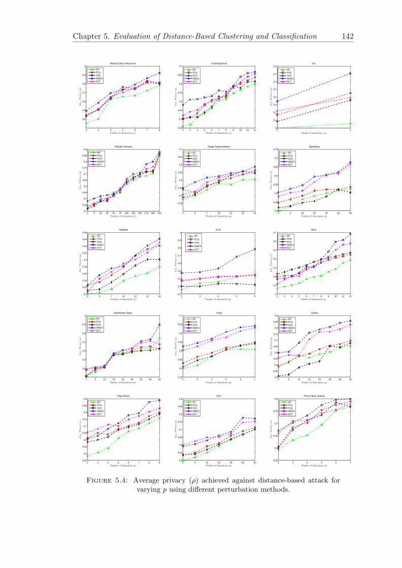
Chapter 5. Evaluation of Distance-Based Clustering and Classification 142
8765432
0.4
0.5
0.6
0.7
0.8
0.9
1
Number of dimensions (p)
Avg
.P
riva
cy(ρ
)
Breast Cancer Wisconsin
RPPCASVDNMDSDCT
121110987654320.35
0.4
0.45
0.5
0.55
0.6
0.65
0.7
Number of dimensions (p)
Avg
.P
riva
cy(ρ
)
Credit Approval
RPPCASVDNMDSDCT
320
0.1
0.2
0.3
0.4
0.5
0.6
0.7
0.8
Number of dimensions (p)
Avg
.P
riva
cy(ρ
)
Iris
RPPCASVDNMDSDCT
21520017515012510075502510520.4
0.45
0.5
0.55
0.6
0.65
0.7
0.75
0.8
0.85
0.9
Number of dimensions (p)
Avg
.P
riva
cy(ρ
)
Multiple Features
RPPCASVDNMDSDCT
18151210752
0.35
0.4
0.45
0.5
0.55
0.6
0.65
0.7
Number of dimensions (p)
Avg
.P
riva
cy(ρ
)
Image Segementation
RPPCASVDNMDSDCT
5040302010520.4
0.45
0.5
0.55
0.6
0.65
0.7
0.75
Number of dimensions (p)
Avg
.P
riva
cy(ρ
)
Spambase
RPPCASVDNMDSDCT
181512107520.3
0.32
0.34
0.36
0.38
0.4
0.42
0.44
0.46
0.48
Number of dimensions (p)
Avg
.P
riva
cy(ρ
)
Hepatitis
RPPCASVDNMDSDCT
654320.2
0.3
0.4
0.5
0.6
0.7
0.8
0.9
1
Number of dimensions (p)
Avg
.P
riva
cy(ρ
)
Ecoli
RPPCASVDNMDSDCT
121110987654320
0.1
0.2
0.3
0.4
0.5
0.6
0.7
Number of dimensions (p)
Avg
.P
riva
cy(ρ
)
Wine
RPPCASVDNMDSDCT
6360504030201052
0.4
0.5
0.6
0.7
0.8
0.9
1
Number of dimensions (p)
Avg
.P
riva
cy(ρ
)
Handwritten Digits
RPPCASVDNMDSDCT
7654320.35
0.4
0.45
0.5
0.55
0.6
0.65
0.7
Number of dimensions (p)
Avg
.P
riva
cy(ρ
)
Yeast
RPPCASVDNMDSDCT
353025201510520.4
0.45
0.5
0.55
0.6
0.65
0.7
0.75
0.8
0.85
0.9
Number of dimensions (p)
Avg
.P
riva
cy(ρ
)
Satlog
RPPCASVDNMDSDCT
987654320.45
0.5
0.55
0.6
0.65
0.7
0.75
0.8
0.85
0.9
Number of dimensions (p)
Avg
.P
riva
cy(ρ
)
Page Blocks
RPPCASVDNMDSDCT
5040302010520.5
0.55
0.6
0.65
0.7
0.75
0.8
0.85
0.9
Number of dimensions (p)
Avg
.P
riva
cy(ρ
)
SCC
RPPCASVDNMDSDCT
7654320.55
0.6
0.65
0.7
0.75
0.8
Number of dimensions (p)
Avg
.P
riva
cy(ρ
)
Pima−indian−diabets
RPPCASVDNMDSDCT
Figure 5.4: Average privacy (ρ) achieved against distance-based attack forvarying p using different perturbation methods.

Chapter 5. Evaluation of Distance-Based Clustering and Classification 143
of V I were low for most datasets compared with the data at lower dimensions,
with the one exception of DCT. The results demonstrate that the accuracy of the
clustering on the perturbed data would be improved as the number of dimensions
increases. However, the variation of clustering becomes more comparable when
suppressing a large number of dimensions.
To jointly assess the utility, which is explained by the accuracy on the perturbed
data, with the privacy, we considered the attacks proposed in Chapter 4. Figure
5.4 shows the average privacy of the distance-based attack achieved at different
dimensions. By comparing Figures 5.1-5.4, it is easy to see that preserving data
utility when the number of dimensions is high could result in good privacy. In
other words, the data at the higher dimensions always preserve both high pro-
tection against the attack and utility for the clustering algorithms. Interestingly,
NMDS outperformed all other methods, achieving better privacy and low cluster-
ing variation particularly at the high dimensions, i.e. the scores of ρ and V I were
on average larger/smaller than those corresponding to other methods, respectively.
This is expected as the larger the number of dimensions included, the more data
utility and the more uncertainty held in the perturbed data. We conclude that
perturbing the data using high dimensionality does not reduce the accuracy of the
distance-based clustering.
Similarly, Figure 5.5 shows the similarity between the original data and the
recovered data using the PCA-based attack. In contrast to the previous attack,
all datasets at high dimensionality display low privacy for all methods because
the attacker would be able to minimise the bias of aligning the eigenvectors of the
know sample and the perturbed data. In contrast, the lower dimensions preserve
more privacy because of the distortion incurred in producing the perturbed data.
Although retaining more features accomplishes more power for discovering clusters,
it may increase the risks of disclosure under this particular attack scenario.
From 5.1, 5.2, 5.3 and 5.5, we can observe that NMDS generally succeeds in
preserving better utility compared to other methods. At the same time, NMDS
preserves acceptable privacy against the PCA-based attack. In addition, the data
at low dimensions have low disclosure risk but that would be on the account
of utility for clustering. The number of dimensions, p, is the critical parameter
of choice in the trade-off between utility and privacy. The choice of p dictates
the extent to which the original data can acceptably be distorted. For instance,
plausible value of V I (0.52) and privacy (3.06) can be achieved using 4 dimensions
for NMDS on the Breast Cancer dataset when DBSCAN is used. As it can be

Chapter 5. Evaluation of Distance-Based Clustering and Classification 144
seen in Figure 5.3, the curve of V I for NMDS goes up for dimensions lower than
4 while relatively remains stable at the higher dimensions.
In summary, the results confirm that NMDS can produce data that of acceptable
quality for distance-based clustering whilst maintain adequate privacy. NMDS can
be seen to outperform other dimensionality reduction techniques by producing very
similar results from the original and perturbed data. NMDS also showed that a
small increase in the number of dimensions, p, can lead to better privacy for
distance-based attack and worse privacy for PCA-based attack. This implies that
the trade-off between privacy and utility may be dependent on the type of attack.
Choosing the right values of p for balancing privacy and utility may require some
risk assessment of the type of attacks expected.

Chapter 5. Evaluation of Distance-Based Clustering and Classification 145
87654322.2
2.4
2.6
2.8
3
3.2
3.4
3.6
Number of dimensions (p)
Avg
.D
ista
nce
Err
or||x
−x||
Breast Cancer Wisconsin
RPPCASVDNMDSDCT
121110987654321.3
1.35
1.4
1.45
1.5
1.55
1.6
1.65
1.7
Number of dimensions (p)
Avg
.D
ista
nce
Err
or||x
−x||
Credit Approval
RPPCASVDNMDSDCT
322.35
2.4
2.45
2.5
2.55
2.6
Number of dimensions (p)
Avg
.D
ista
nce
Err
or||x
−x||
Iris
RPPCASVDNMDSDCT
21520017515012510075502510521.35
1.4
1.45
1.5
1.55
Number of dimensions (p)
Avg
.D
ista
nce
Err
or||x
−x||
Multiple Features
RPPCASVDNMDSDCT
181512107521.55
1.6
1.65
1.7
1.75
1.8
1.85
1.9
Number of dimensions (p)
Avg
.D
ista
nce
Err
or||x
−x||
Image Segementation
RPPCASVDNMDSDCT
5040302010522.44
2.46
2.48
2.5
2.52
2.54
2.56
2.58
2.6
2.62
2.64
Number of dimensions (p)
Avg
.D
ista
nce
Err
or||x
−x||
Spambase
RPPCASVDNMDSDCT
181512107522.58
2.6
2.62
2.64
2.66
2.68
2.7
2.72
2.74
2.76
Number of dimensions (p)
Avg
.D
ista
nce
Err
or||x
−x||
Hepatitis
RPPCASVDNMDSDCT
654322.5
2.55
2.6
2.65
2.7
2.75
2.8
2.85
2.9
Number of dimensions (p)
Avg
.D
ista
nce
Err
or||x
−x||
Ecoli
RPPCASVDNMDSDCT
121110987654321.4
1.5
1.6
1.7
1.8
1.9
2
Number of dimensions (p)
Avg
.D
ista
nce
Err
or||x
−x||
Wine
RPPCASVDNMDSDCT
63605040302010522.7
2.75
2.8
2.85
2.9
2.95
3
Number of dimensions (p)
Avg
.D
ista
nce
Err
or||x
−x||
Handwritten Digits
RPPCASVDNMDSDCT
765432
2.7
2.75
2.8
2.85
2.9
Number of dimensions (p)
Avg
.D
ista
nce
Err
or||x
−x||
Yeast
RPPCASVDNMDSDCT
353025201510521.56
1.58
1.6
1.62
1.64
1.66
1.68
1.7
1.72
Number of dimensions (p)
Avg
.D
ista
nce
Err
or||x
−x||
Satlog
RPPCASVDNMDSDCT
987654322.45
2.5
2.55
2.6
2.65
2.7
2.75
2.8
2.85
Number of dimensions (p)
Avg
.D
ista
nce
Err
or||x
−x||
Page Blocks
RPPCASVDNMDSDCT
5040302010522.35
2.4
2.45
2.5
Number of dimensions (p)
Avg
.D
ista
nce
Err
or||x
−x||
SCC
RPPCASVDNMDSDCT
7654322.55
2.6
2.65
2.7
2.75
2.8
Number of dimensions (p)
Avg
.D
ista
nce
Err
or||x
−x||
Pima−indian−diabets
RPPCASVDNMDSDCT
Figure 5.5: Average privacy achieved against PCA-based attack for varying pusing different perturbation methods.

Chapter 5. Evaluation of Distance-Based Clustering and Classification 146
5.3 Application to Classification Tasks
5.3.1 k-Nearest Neighbours (k-NN)
k-NN [37] is one of the traditional techniques that are used to extract classification
patterns within data. The major task of k-NN is to classify each unlabelled exam-
ple by the majority label of its k-nearest neighbours in the training set. As we have
seen in chapter 2, the notion of nearness or equivalently closeness is determined
by learning an appropriate distance metric between different examples. When the
value of k is relatively large, the algorithm may include some objects that are not
so similar to the target object. Whereas, a smaller k may exclude some potential
candidate objects. This indeed will lead to low classification accuracy. Therefore,
many approaches have been suggested to reduce the impact of k using different
techniques. For example, a distance-weighted constraint was proposed in [53]. The
general steps of the k-NN classification are summarised as follows:
1. Define a suitable distance metric.
2. Find the k nearest neighbours using the defined distance metric.
3. Find the class of the k-nearest neighbours and vote on the majority class.
4. Assign that class to the example to be classified.
The nearest neighbour rule can mathematically be described as follows. Given
a set of training objects X = {x1, x2, . . . , xm} and a predefined set of classes
C = {c1, c2, . . . , cs}. Let k be the number of nearest neighbours and Uk be the set
of k closest training examples to a test example x′, the k-NN classification rule of
the test object x′ is defined by
g(x′, c′j) = argmaxj
∑(xi,cj)∈Uk
I(j = cj), (5.9)
where
I(.) =
1 if the argument (.) is true,
0 otherwise.
The object xi is said to be the kth nearest neighbour of x′ when ||xi − x′|| is
the kth smallest among ||x1 − x′||, ||x2 − x′||, . . . , ||xn − x′||. The above rule (5.9)
simply implies the majority voting on the class of the test example, x′.

Chapter 5. Evaluation of Distance-Based Clustering and Classification 147
5.3.2 Support Vector Machine (SVM)
The foundations of SVM have been developed by Vapnik [169], and are gaining
popularity in machine learning due to its attractive features and its promising re-
sults [22, 51, 84]. The basic idea is to find a hyperplane that separates the data into
two classes with as great a margin as possible. The optimal hyperplane (decision
boundary) is the one that separates these two classes and that maximises the dis-
tance between the two closest points from either class (known as support vectors).
Assume that the classes of data are separable. Consider a binary classification
problem consisting of m pairs of training examples (x1, y1), (x2, y2), . . . , (xm, ym),
where xi ∈ Rn and yi ∈ {−1, 1}; the hyperplane is defined by
w · x + b = 0, (5.10)
where w is the weight vector and b is the bias. The symbol “.” denotes the dot
product in the feature space. Both parameters w and b must be chosen in such a
way that the following two conditions are met:
w · xi + b ≥ 1 when yi = 1, and
w · xi + b ≤ −1 when yi = −1.(5.11)
The classification rule of an unseen test object x′ is defined by
g(x′) = sign(w · x′ + b). (5.12)
Maximising the distance from a point x to the hyperplane in (5.10) determines
the optimal hyperplane which creates the maximal margin between the negative
and positive training examples (Figure 5.6(a)). The distance from a hyperplane
H(w, b) to a given data point xi is simply
d(H(w, b),xi) =w · xi + b
||w|| ≥ 1
||w|| . (5.13)
That is, SVM finds the hyperplane that maximises the margin by minimising
the squared norm of the hyperplane
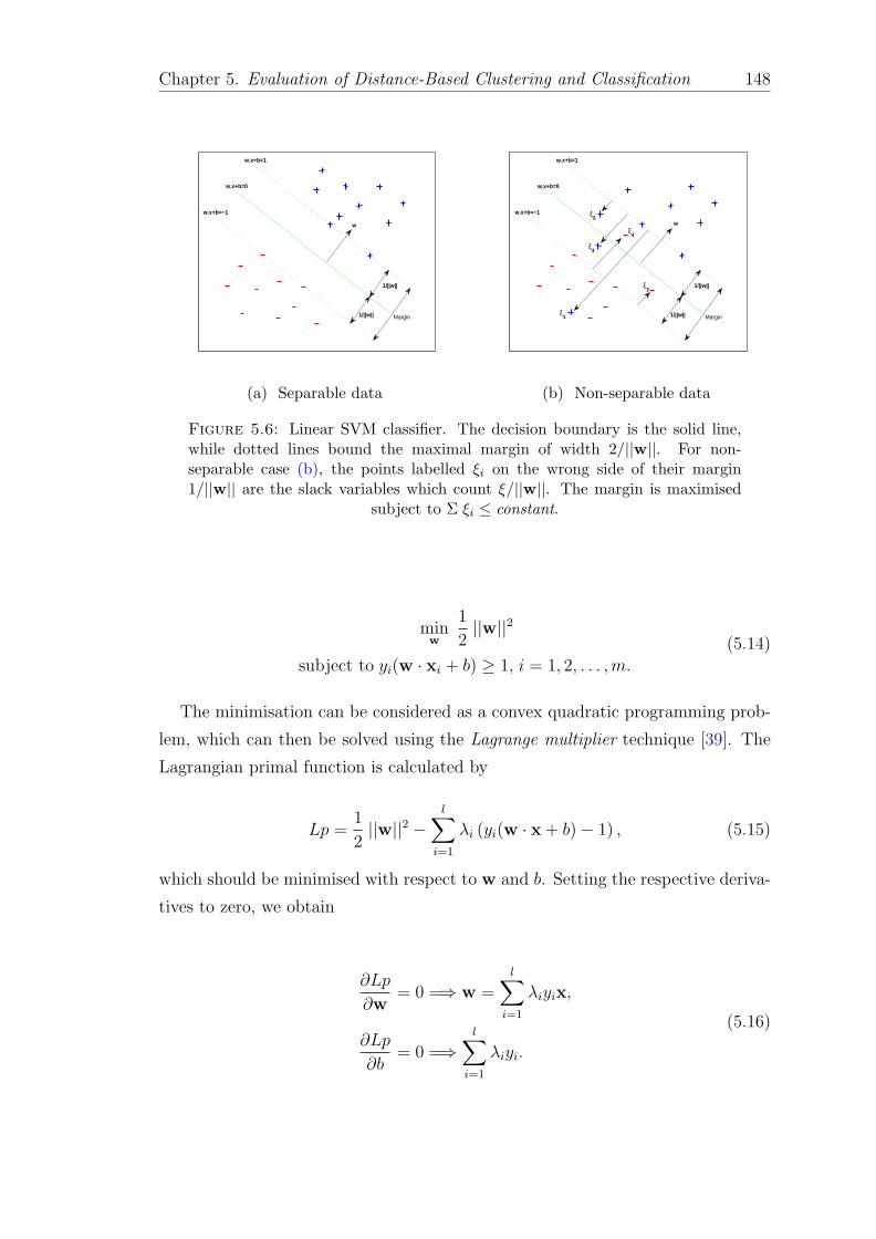
Chapter 5. Evaluation of Distance-Based Clustering and Classification 148
1/||w||
1/||w||
w.x+b=1
w.x+b=0
w.x+b=−1
Margin
w
(a) Separable data
1/||w||
1/||w||
w.x+b=1
w.x+b=0
w.x+b=−1
Margin
wξ
4
ξ3
ξ5
ξ1
ξ2
(b) Non-separable data
Figure 5.6: Linear SVM classifier. The decision boundary is the solid line,while dotted lines bound the maximal margin of width 2/||w||. For non-separable case (b), the points labelled ξi on the wrong side of their margin1/||w|| are the slack variables which count ξ/||w||. The margin is maximised
subject to Σ ξi ≤ constant.
minw
1
2||w||2
subject to yi(w · xi + b) ≥ 1, i = 1, 2, . . . ,m.(5.14)
The minimisation can be considered as a convex quadratic programming prob-
lem, which can then be solved using the Lagrange multiplier technique [39]. The
Lagrangian primal function is calculated by
Lp =1
2||w||2 −
l∑i=1
λi (yi(w · x + b)− 1) , (5.15)
which should be minimised with respect to w and b. Setting the respective deriva-
tives to zero, we obtain
∂Lp
∂w= 0 =⇒ w =
l∑i=1
λiyix,
∂Lp
∂b= 0 =⇒
l∑i=1
λiyi.
(5.16)

Chapter 5. Evaluation of Distance-Based Clustering and Classification 149
The problem can be simplified into a function of multipliers only, i.e., dual
Lagrangian, by substituting the above derivatives into Equation (5.15),
Lp =l∑
i=1
λi −1
2λiλjyiyjxi · xj. (5.17)
For non-separable data (Figure 5.6(b)), SVM can also deal with overlapping
classes by maximising the margin, allowing any misclassified data points to be
penalised using a method known as the soft margin approach [172]. The misclassi-
fication bias can be defined by the so-called slack variables, ξ = ξ1, ξ2, . . . , ξs. Let
ξi ≥ 0; the constraints of the optimisation can be rewritten as
w · xi + b ≥ 1− ξi when yi = 1, and
w · xi + b ≤ −1 + ξi when yi = −1,(5.18)
and the learning task in SVM can be formalised as follows:
minw
1
2||w||2 + C
l∑i=1
ξi
subject to
yi(w · xi + b) ≥ 1− ξi, i = 1, 2, . . . ,m,
ξi ≥ 0, Σ ξi ≤ C
(5.19)
where the constant C is a regularisation parameter used to create a balance be-
tween a maximum margin and a small number of misclassified data points.
The SVM described so far finds linear boundaries in the input space. However,
in many real problems, data may have non-linear decision boundaries, which would
make finding a hyperplane that can successfully separate two overlapping classes a
difficult task. One solution to this problem is to use the so-called kernel trick. The
trick here is to transform the data X in d-dimensional input space into a higher
D-dimensional feature space F (also known as Hilbert space), Φ : Rd → RD where
D � d. This would make the overlapping classes separable in the new space F .
The transformation is performed via a kernel function K that satisfies Mercer’s
condition [170] so that better class separation can be achieved [38]. The function
K can be defined by
K(u,v) = Φ(u) · Φ(v), (5.20)

Chapter 5. Evaluation of Distance-Based Clustering and Classification 150
where Φ : X → F and “.” denotes the dot product in the feature space F . By
defining a proper K, we simply replace all occurrences of xi in the SVM model
with Φ(xi). That is, the feature space F is never explicitly dealt with, but rather
we evaluate the dot product, Φ(xi) . Φ(xj), directly using function K in the input
space [144]. Intuitively, computing only the dot product using K, in the feature
space, is substantially cheaper than using the transformed attributes. For example,
the radial basis function kernel unfolds into an infinite-dimension Hilbert space.
5.3.3 Utility Measures for Classification
To guarantee the best performance of the distance-based classifiers, we need a
transformation that provides a faithful mapping (with minimum preservation er-
ror) for a given dataset in which the distances between neighbouring points are
approximately unchanged and the underlying structure is revealed. That is, ob-
jects that are close to each other are close to each other after the transformation.
Measuring the average distance difference between objects in the input and
output spaces may indicate the size of information loss as a results of the trans-
formation. As discussed in Chapter 4, this difference can be quantified using the
stress (4.3). Broadly speaking, minimising the stress may lead to better utility of
the perturbed data for distance-based analysis. However, to assess the “goodness”
of the perturbed data for classification analysis, we may also measure the change
of the underlying data structure. For this purpose, we define two further utility
measures. The first measure, Neighbourhood Preservation (NP), aims at quantify-
ing the impact of the perturbation on the structure of the neighbourhood points.
To provide higher data utility, for each data point in the perturbed data the k
neighbourhood points should be the same as the k neighbourhood points in the
original data. The second measure, Class Compactness (CC), aims at quantifying
the impact of the perturbation on the class distribution. Here, we would like to
ensure that for each data point with class ci, the number of the k neighbourhood
points with the same class should be the same before and after the perturbation.
A higher score for both measures represents higher data quality. Measures that
correspond to those properties are described in the following subsections.

Chapter 5. Evaluation of Distance-Based Clustering and Classification 151
X
(a) Original data
X
(b) Perturbed data
Figure 5.7: The impact of the transformation on classifying example x wherethe distances of 3-nearest neighbours have been changed. In the original data(a), the example is classified as “negative” whereas in the perturbed data (b) it
is classified as “positive”.
5.3.3.1 Neighbourhood Preservation
Preserving the topological structure of data in the lower dimensional space may
demonstrate the usefulness of the data for analysis or visualisation. The neighbour-
hood is preserved if the distribution of the k-nearest neighbours, in the original
space, X, is unchanged or well approximated in the perturbed space, Y [171].
That is, points in X are mapped to points in Y , such that nearby points and
faraway points are still nearby and faraway, respectively.
When the pairwise distances are distorted as a result of the transformation,
the accuracy of the classifier is likely to decrease. To illustrate this, consider the
example in Figure 5.7. Assume that k = 3. Unlabelled test object x, located
at the centre of the circle, will be classified based on the majority class label of
its k-neighbours training objects, which belong to either a “+” or “−” class. In
the original data (Figure 5.7(a)), the point is classified as a “−” example because
the majority class of its neighbours is negative. However, in the perturbed data
(Figure 5.7(b)), the point will be classified as “+” for the same reason. Thus,
the quantification of the neighbourhood preservation in the new space can be an
indicator of utility for distance-based classification analysis. Let m be the number
of data objects and k be the number of neighbours, the quality of neighbourhood
preservation [62] can be measured by

Chapter 5. Evaluation of Distance-Based Clustering and Classification 152
NP =1
k
m∑i=1
|Uk(xi) ∩ Uk(yi)|m
, (5.21)
where Uk(xi) and Uk(yi) are sets of the k-nearest neighbours of point xi, in the
original data, X, and point yi, in the perturbed data, Y , respectively.
This measure indeed quantifies, for each point, the size of the intersection of the
set of k neighbours in the original space, X, and in the perturbed space, Y . Hence,
it should be maximised. If the maximum value of this measure is one, the resulting
new space is clearly useful for analysis, as the distances of the neighbourhoods are
well preserved.
5.3.3.2 Class Compactness
Since the distance metric plays an important role in distance-based learning,
changing distance measurements between objects due to the transformation will
influence the behaviour of the classifier and thereby will decrease the accuracy. If
members of the same class are close to each other in the original data space, they
should also be close to each other in the perturbed data space, i.e. the cluster
they belong to should be compact and separable from other clusters. This prop-
erty indicates that the distance between any two points in different groups should
be larger than the distance between any two points within the group.
Given a set of objects X = {x1, x2, . . . , xm} and a predefined set of classes
C = {c1, c2, . . . , cs}, class compactness [62] for any class cj ∈ C is defined by
CCj =1
k
∑xi∈cj
|Uk(xi, cj)|m(cj)
, (5.22)
where Uk(xi, j) is a set of the k-nearest neighbours of point xi having class label
cj, and m(cj) is the number of points in class cj. The overall class compactness is
CC =1
s
s∑j=1
CCj. (5.23)
The class compactness measure evaluates how well the different groups within
the original data are redistributed in the perturbed space. In other words, it
assesses the local homogeneity of the objects within each group. A low value of
this measure indicates high variance of group membership. In contrast, a better
preservation of the underlying class structure can be achieved when the value is
close to one.

Chapter 5. Evaluation of Distance-Based Clustering and Classification 153
5.3.4 Experimental Results
In this section, we show some empirical results that illustrate the impact of pertur-
bation using different transforms on the accuracy of distance-based classification.
To examine the quality of classification, we compare the quality of accuracy ob-
tained from the original data, X, and the perturbed data, Y at different reduced
dimensions (Section 5.3.4.2). If the misclassification error of the classifier that is
trained on Y is equal to that error from the classifier on X, then the transforma-
tion, T , causes low distortion and thereby a good data utility is preserved. This
implies that the classifier on Y is invariant to T .
In Section 5.3.4.3, we assess the utility in terms of preserving the underlying
structure of the perturbed data using NP and CC measures which are described
in Section 5.3.3. We also evaluate the trade-off between privacy and utility in
the perturbed data (Section 5.3.4.4). Finally, we test the performance difference
between the used perturbation techniques to find out whether or not the proposed
technique (NMDS) performs significantly better than other techniques (Section
5.3.4.5).
5.3.4.1 Experimental Setup
We conducted our classification experiments on the same 15 datasets used earlier
in Section 5.2. The classifiers used are MATLAB implementations of k-NN, lin-
ear SVM and non-linear SVM with three popular kernels (Polynomial, Gaussian
Radial Basis Function (RBF) and Multilayer Perceptron). The original data are
projected into several lower dimensional spaces in order to produce the perturbed
data using five different transforms (RP, PCA, SVD, NMDS and DCT). Then,
we used the perturbed data, Y , in p-dimensional space, to carry out the classi-
fication and to compare it with the results obtained from the original data, X.
We computed the classification accuracy on the original data as a baseline for
comparison.
To estimate the accuracy of the k-NN classifier on both X and Y , we used
10-fold cross-validation over 30 runs, the results are then averaged. The value of
k was set to 4 and the number of dimensions, p, was varied in a consistent manner
based on the total number of attributes. We used 70% of the data for training
and tested the classifier on the 30% remaining data. To avoid the randomisation
caused by RP when producing the random matrix, we chose to use an average of
20 runs and choose the one with the lowest stress.

Chapter 5. Evaluation of Distance-Based Clustering and Classification 154
For SVM classification, we also we used 10-fold cross-validation and the average
classification accuracy is calculated over 30 trials. For simplicity, we used datasets
with a binary class, i.e. positive and negative groups. The error rates of the testing
set were evaluated for both data X and Y .
The regularisation parameter, C, was set to 1 in all experiments. We consider
this adequate as in this set of experiments our main concern is to compare the
SVM models obtained with the original and perturbed data and not to get the
optimal SVM model, therefore we do not experiment with the parameters of SVM.
However, C is an important parameter in SVMs which needs to be set correctly. In
general, higher values of C may lead to more accurate results, while lower values
correspond to a more flexible hyperplane where the misclassification error is less
important [76]. That is, varying the value of C may result in different performance.
The parameters of the kernels were set as follows: The degree of Polynomial
function set to 3, the radius of RBF set to 1 and the Sigmoid kernel function of
the Multilayer Perceptron set with a slope equals 1 and intercept equals -1.
In order to compare the performance of the classification algorithms over all
datasets, we used Friedman test [46]. In this test, each transform is ranked for
each dataset separately, according to the achieved accuracy, in ascending order,
from the best performing transform (getting the rank of 1) to the worse performing
transform (getting the rank of N , where N is the number of the compared trans-
forms). If two or more transforms have the same accuracy, then their ranks are
averaged. Then we calculated the mean rank for each transform on all datasets.
This may indicate the relative performance over all the datasets while the ranking
themselves may provide a fair comparison of the transforms.
The Friedman test typically checks whether the measured average ranks are
significantly different from the mean rank. The null hypotheses (H0) is all trans-
forms are equal in their performance, i.e. there is no difference in mean ranks for
repeated measures.
To further illustrate the significant difference in the average ranks of the five
transforms, we used the critical difference (CD) diagram [46] with a significance
level of α = 5%. This diagram provides a graphical representation of the overall
performance where statistically similar transforms are linked together by cliques
and each single clique is represented by a solid bar.

Chapter 5. Evaluation of Distance-Based Clustering and Classification 155
5.3.4.2 Comparing Accuracy of Classifiers
The mean classification accuracy of k-NN classifier is shown in Figure 5.8. Gener-
ally, for all datasets, it is clear that as p increases, the classification error decreases.
With decreasing p, it is expected that pairwise distances in the perturbed data
will get distorted and it will be more difficult to classify objects correctly. The
accuracies of k-NN classifier on the perturbed data produced by NMDS and PCA
are approximately the same as on the original data (even better in some cases)
particularly at high dimensions. Additionally, the performance of k-NN classifier
on the perturbed data produced by NMDS is the highest compared with other
transforms. The worse performance is reported for DCT where the accuracy is
the lowest. PCA gives a performance quite similar to NMDS in most cases. The
results show a significant decrease in accuracy for p < 2 for the datasets with a
few number of dimensions, and for p < 10 for the datasets with a large number of
dimensions.
Figure 5.9 shows the classification accuracy of linear SVM on the perturbed
data produced by NMDS at different dimensions against those of RP, PCA, SVD
and DCT. The algorithm performs well on the data produced by RP, PCA, SVD
and NMDS as the accuracy is close to the accuracy on the original data, X,
particularly when retaining a large number of dimensions. The worse performing
was on the data produced by DCT with an average accuracy of 0.07% lower than
other methods. However, linear SVM on DCT data shows a stable performance at
all dimensions. In general, the accuracies for RP, PCA, SVD and NMDS remain
apparently unchanged too much at the very lower dimensions. This implies that
SVM is able to separate non-separable classes even at low dimensions for the data
produced by these methods. One exception is shown for Pima Diabetes dataset
where the change of accuracy at lower dimensions is noticeable.
The majority of the transforms used, with the exception of DCT, achieve an
accuracy in the regions of 93-98% for BCW, 75-86% for Credit Approval, 72-77%
for Pima Diabetes, 83-86% for Hepatitis and 88-92% for Spambase. However, the
linear SVM performs slightly better on the data produced by NMDS, particularly
at high dimensions. The results also indicate using DCT results in deteriorated
performance as the accuracy compared with the other transforms is markedly
lower. However, we observe a slight improvements in accuracy on the SVD data
which is quite close the performance on the PCA and NMDS data.
Figure 5.10 shows the average classification accuracy of non-linear Linear SVM
using three different kernels at several reduced dimensions. Here, we observe that
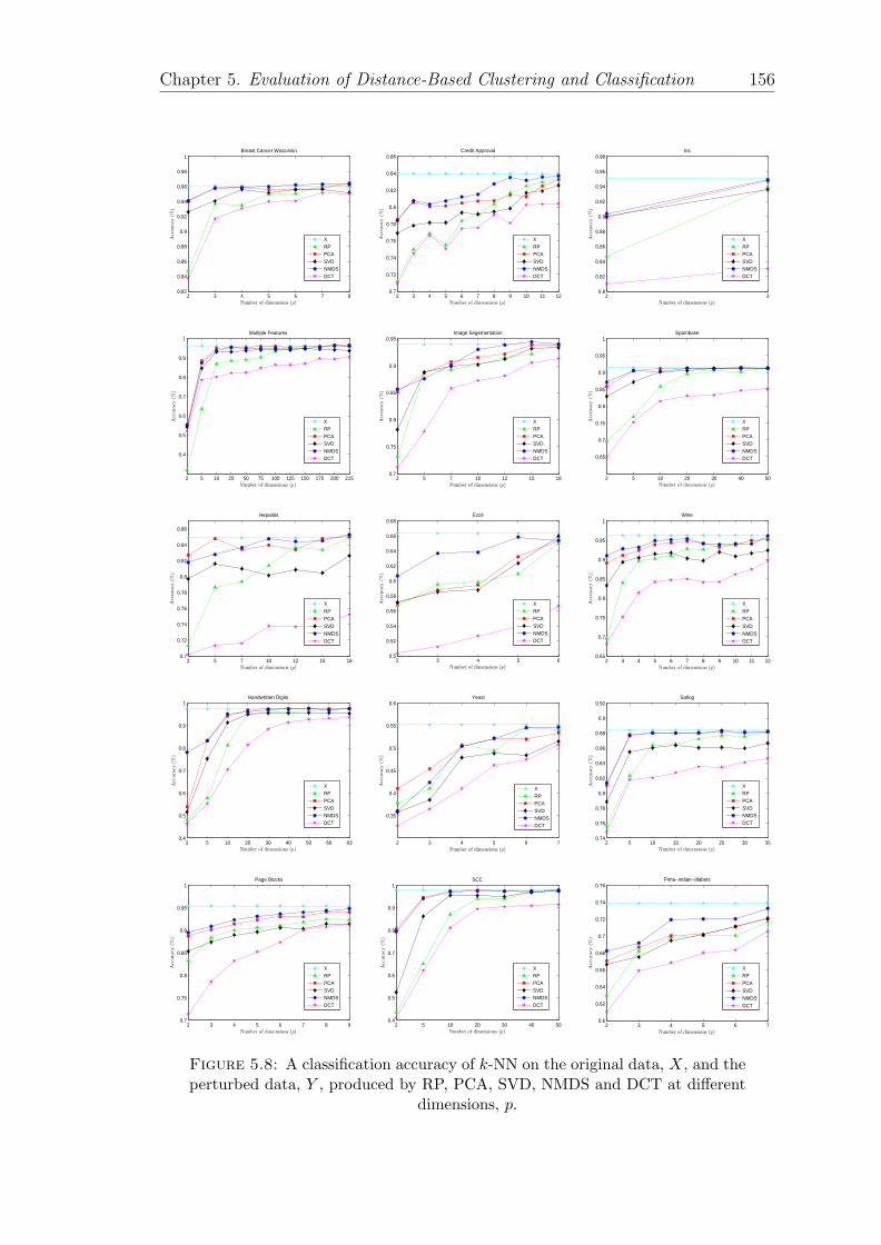
Chapter 5. Evaluation of Distance-Based Clustering and Classification 156
87654320.82
0.84
0.86
0.88
0.9
0.92
0.94
0.96
0.98
1
Number of dimensions (p)
Acc
urac
y(%
)
Breast Cancer Wisconsin
XRPPCASVDNMDSDCT
121110987654320.7
0.72
0.74
0.76
0.78
0.8
0.82
0.84
0.86
Number of dimensions (p)
Acc
urac
y(%
)
Credit Approval
XRPPCASVDNMDSDCT
320.8
0.82
0.84
0.86
0.88
0.9
0.92
0.94
0.96
0.98
Number of dimensions (p)
Acc
urac
y(%
)
Iris
XRPPCASVDNMDSDCT
2152001751501251007550251052
0.4
0.5
0.6
0.7
0.8
0.9
1
Number of dimensions (p)
Acc
urac
y(%
)
Multiple Features
XRPPCASVDNMDSDCT
181512107520.7
0.75
0.8
0.85
0.9
0.95
Number of dimensions (p)
Acc
urac
y(%
)
Image Segementation
XRPPCASVDNMDSDCT
504030201052
0.65
0.7
0.75
0.8
0.85
0.9
0.95
1
Number of dimensions (p)
Acc
urac
y(%
)
Spambase
XRPPCASVDNMDSDCT
181512107520.7
0.72
0.74
0.76
0.78
0.8
0.82
0.84
0.86
Number of dimensions (p)
Acc
urac
y(%
)
Hepatitis
XRPPCASVDNMDSDCT
654320.5
0.52
0.54
0.56
0.58
0.6
0.62
0.64
0.66
0.68
Number of dimensions (p)
Acc
urac
y(%
)
Ecoli
XRPPCASVDNMDSDCT
121110987654320.65
0.7
0.75
0.8
0.85
0.9
0.95
1
Number of dimensions (p)
Acc
urac
y(%
)
Wine
XRPPCASVDNMDSDCT
63605040302010520.4
0.5
0.6
0.7
0.8
0.9
1
Number of dimensions (p)
Acc
urac
y(%
)
Handwritten Digits
XRPPCASVDNMDSDCT
765432
0.35
0.4
0.45
0.5
0.55
0.6
Number of dimensions (p)
Acc
urac
y(%
)
Yeast
XRPPCASVDNMDSDCT
353025201510520.74
0.76
0.78
0.8
0.82
0.84
0.86
0.88
0.9
0.92
Number of dimensions (p)
Acc
urac
y(%
)
Satlog
XRPPCASVDNMDSDCT
987654320.7
0.75
0.8
0.85
0.9
0.95
1
Number of dimensions (p)
Acc
urac
y(%
)
Page Blocks
XRPPCASVDNMDSDCT
5040302010520.4
0.5
0.6
0.7
0.8
0.9
1
Number of dimensions (p)
Acc
urac
y(%
)
SCC
XRPPCASVDNMDSDCT
7654320.6
0.62
0.64
0.66
0.68
0.7
0.72
0.74
0.76
Number of dimensions (p)
Acc
urac
y(%
)
Pima−indian−diabets
XRPPCASVDNMDSDCT
Figure 5.8: A classification accuracy of k-NN on the original data, X, and theperturbed data, Y , produced by RP, PCA, SVD, NMDS and DCT at different
dimensions, p.

Chapter 5. Evaluation of Distance-Based Clustering and Classification 157
87654320.8
0.82
0.84
0.86
0.88
0.9
0.92
0.94
0.96
0.98
Number of dimensions (p)
Acc
urac
y(%
)
Breast Cancer Wisconsin
XRPPCASVDNMDSDCT
121110987654320.65
0.7
0.75
0.8
0.85
0.9
Number of dimensions (p)
Acc
urac
y(%
)
Credit Approval
XRPPCASVDNMDSDCT
7654320.69
0.7
0.71
0.72
0.73
0.74
0.75
0.76
0.77
0.78
Number of dimensions (p)
Acc
urac
y(%
)
Pima−indian−diabets
XRPPCASVDNMDSDCT
181512107520.81
0.82
0.83
0.84
0.85
0.86
0.87
0.88
0.89
Number of dimensions (p)
Acc
urac
y(%
)
Hepatitis
XRPPCASVDNMDSDCT
5040302010520.78
0.8
0.82
0.84
0.86
0.88
0.9
0.92
Number of dimensions (p)
Acc
urac
y(%
)
Spambase
XRPPCASVDNMDSDCT
Figure 5.9: Classification accuracy of linear SVM at different dimensions, p,using the original data, X, and the perturbed data, Y , produced by RP, PCA,
SVD, NMDS and DCT.
there is an increase in the accuracy whenever the number of dimensions decreases.
This implies that suppressing many dimensions may preserve the quality of non-
linear SVM classification.
The results suggest that the performance of the kernel functions are affected by
the number of dimensions. Reducing the dimensions of data can help the kernel
functions to find better mapping in the feature space and thus better class separa-
tion can be achieved. For instance, when reducing the number of dimensions, p, up
to 50% or less from the total number of dimensions for BCW, Pima Diabetes, Hep-
atitis and Spambase datasets, the accuracies of the classifier substantially increase
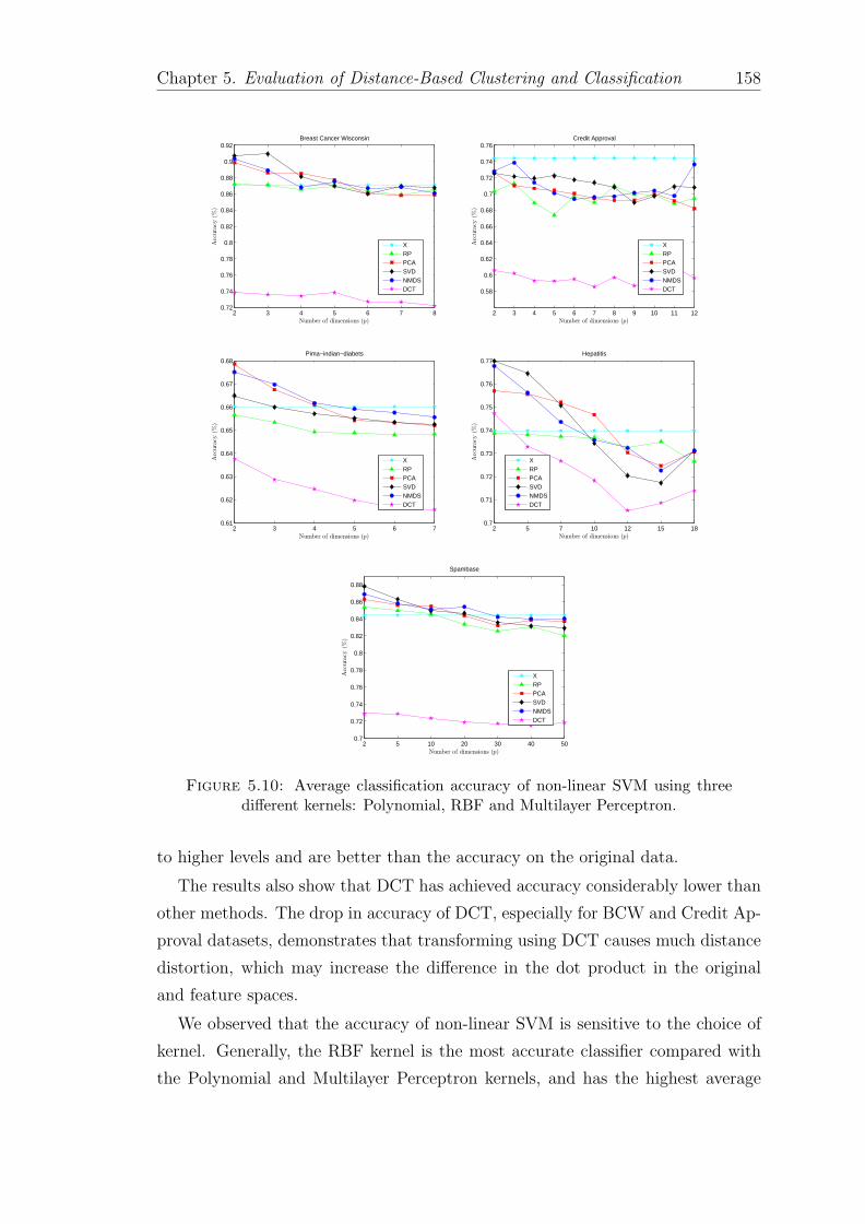
Chapter 5. Evaluation of Distance-Based Clustering and Classification 158
87654320.72
0.74
0.76
0.78
0.8
0.82
0.84
0.86
0.88
0.9
0.92
Number of dimensions (p)
Acc
urac
y(%
)
Breast Cancer Wisconsin
XRPPCASVDNMDSDCT
12111098765432
0.58
0.6
0.62
0.64
0.66
0.68
0.7
0.72
0.74
0.76
Number of dimensions (p)
Acc
urac
y(%
)
Credit Approval
XRPPCASVDNMDSDCT
7654320.61
0.62
0.63
0.64
0.65
0.66
0.67
0.68
Number of dimensions (p)
Acc
urac
y(%
)
Pima−indian−diabets
XRPPCASVDNMDSDCT
181512107520.7
0.71
0.72
0.73
0.74
0.75
0.76
0.77
Number of dimensions (p)
Acc
urac
y(%
)
Hepatitis
XRPPCASVDNMDSDCT
5040302010520.7
0.72
0.74
0.76
0.78
0.8
0.82
0.84
0.86
0.88
Number of dimensions (p)
Acc
urac
y(%
)
Spambase
XRPPCASVDNMDSDCT
Figure 5.10: Average classification accuracy of non-linear SVM using threedifferent kernels: Polynomial, RBF and Multilayer Perceptron.
to higher levels and are better than the accuracy on the original data.
The results also show that DCT has achieved accuracy considerably lower than
other methods. The drop in accuracy of DCT, especially for BCW and Credit Ap-
proval datasets, demonstrates that transforming using DCT causes much distance
distortion, which may increase the difference in the dot product in the original
and feature spaces.
We observed that the accuracy of non-linear SVM is sensitive to the choice of
kernel. Generally, the RBF kernel is the most accurate classifier compared with
the Polynomial and Multilayer Perceptron kernels, and has the highest average

Chapter 5. Evaluation of Distance-Based Clustering and Classification 159
accuracy. The worse performance is reported for the Multilayer Perceptron ker-
nel, particularly at high dimensions. However, we observed that the Multilayer
Perceptron kernel performs better with the decreases of the number of dimensions.
Our experimental results reveal that the proposed technique, i.e. NMDS, is
able to offer competitive classification results on the perturbed data with respect
to the other dimensionality reduction methods (RP, PCA, SVD and DCT). The
important observation is that retaining as many dimensions as possible can signif-
icantly reduce the generalisation error (error on the test data) when using k-NN
and linear SVM. However, this is not true for non-linear SVM as we notice a
decrease in the error when few dimensions are used.
5.3.4.3 Data Utility Measures
To examine whether or not the perturbed data are useful for classification analysis,
we measure the quality of the underlying structure using the measures defined in
Section 5.3.3. In the first set of experiments, we evaluate the impact of number
of dimensions on the neighbourhood preservation and class compactness. We
generate three synthetic groups of 1000 random samples in 100-dimensional space
and normalised the data so all variables have zero mean and standard deviation
equal to one. The data are then transformed into different dimensions, p, using
the five perturbation techniques. For each subset of the data, we measure the
change in neighbourhood structure and class compactness when k = 4. This is
illustrated in Figure 5.11.
The results presented in Figure 5.11(a) show that as the number of dimensions
increases the change in the neighbourhood structure decreases, i.e. NP increases,
for all methods except for DCT which gives a constant performance at all dimen-
sions. NMDS appears to preserve the neighbourhood of data points slightly better
than the other methods. The PCA performs quite similarly to NMDS. The differ-
ence in the neighbourhood preservation from the highest dimension (p = 100) to
the lowest dimension (p = 10) is 0.70 for RP, PCA and NMDS while SVD shows
relatively low variation where the difference is approximately 0.15.
The results presented in Figure 5.11(b) suggest that the perturbations caused
by RP, PCA, SVD and NMDS have not seriously destroyed the structure of the
classes’ distributions as all these methods successfully preserve the class compact-
ness, although the change seems slightly higher for RP and SVD at p = 10. DCT
exhibits noticeably worse performance compared with the other methods. For in-
stance, the class compactness in the perturbed data produced by DCT at p = 100

Chapter 5. Evaluation of Distance-Based Clustering and Classification 160
10 20 30 40 50 60 70 80 90 1000.2
0.3
0.4
0.5
0.6
0.7
0.8
0.9
1
Number of dimensions (p)
Nei
ghbo
urho
odP
rese
rvat
ion
(NP
)
RPPCASVDNMDSDCT
(a)
10 20 30 40 50 60 70 80 90 1000.5
0.55
0.6
0.65
0.7
0.75
0.8
0.85
0.9
0.95
1
Number of dimensions (p)
Cla
ssC
ompa
ctne
ss(C
C)
RPPCASVDNMDSDCT
(b)
Figure 5.11: (a) Neighbourhood preservation and (b) class compactness atdifferent dimensions in the perturbed data, Y , using different perturbation tech-
niques.
is 0.58 while the average class compactness for the other methods at the same
dimensions is 0.95. Again, both PCA and NMDS perform quite similarly at all
dimensions.
We can conclude that retaining as many dimensions as possible in the perturbed
space results in significantly less information loss with respect to neighbourhood
preservation. However, this my not hold for class compactness as eliminating
many dimensions does not have an effect on preserving the classes’ distributions,
particularly when k = 4. Overall, the perturbed data, produced by RP, PCA and
NMDS, at the high dimensions often preserve the underlying properties and thus
provide high data utility for distance-based classification.
To examine the effect of the number of neighbours, k, we calculate the neigh-
bourhood preservation and the class compactness of the data at 99-dimensional
space, which represents the best fit of the original dimensional space. The values
of k were varied from 3 to 10. The results of neighbourhood preservation are
shown in Tables 5.6 and the results of class compactness are shown in Table 5.7.
The results suggest that whenever the value of k increases, the neighbourhood
preservation and class compactness become relatively smaller. This can clearly
be noticed from the results for SVD and DCT. The other methods including RP,
PCA and NMDS show better performance even when using large number of k.
For the real dataset, we also evaluate the utility of the perturbed data using
different number of neighbours, k, to examine if there exists a variation in neigh-
bourhood structure and class compactness as a result of mapping data points from
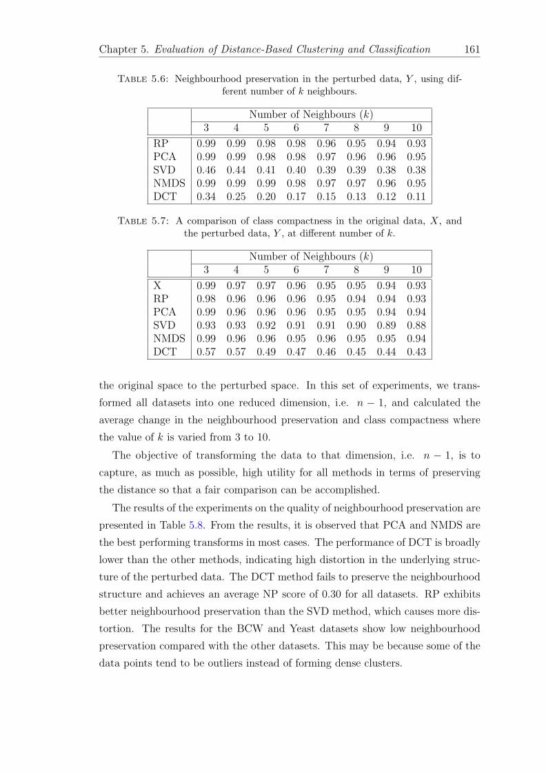
Chapter 5. Evaluation of Distance-Based Clustering and Classification 161
Table 5.6: Neighbourhood preservation in the perturbed data, Y , using dif-ferent number of k neighbours.
Number of Neighbours (k)3 4 5 6 7 8 9 10
RP 0.99 0.99 0.98 0.98 0.96 0.95 0.94 0.93PCA 0.99 0.99 0.98 0.98 0.97 0.96 0.96 0.95SVD 0.46 0.44 0.41 0.40 0.39 0.39 0.38 0.38NMDS 0.99 0.99 0.99 0.98 0.97 0.97 0.96 0.95DCT 0.34 0.25 0.20 0.17 0.15 0.13 0.12 0.11
Table 5.7: A comparison of class compactness in the original data, X, andthe perturbed data, Y , at different number of k.
Number of Neighbours (k)3 4 5 6 7 8 9 10
X 0.99 0.97 0.97 0.96 0.95 0.95 0.94 0.93RP 0.98 0.96 0.96 0.96 0.95 0.94 0.94 0.93PCA 0.99 0.96 0.96 0.96 0.95 0.95 0.94 0.94SVD 0.93 0.93 0.92 0.91 0.91 0.90 0.89 0.88NMDS 0.99 0.96 0.96 0.95 0.96 0.95 0.95 0.94DCT 0.57 0.57 0.49 0.47 0.46 0.45 0.44 0.43
the original space to the perturbed space. In this set of experiments, we trans-
formed all datasets into one reduced dimension, i.e. n − 1, and calculated the
average change in the neighbourhood preservation and class compactness where
the value of k is varied from 3 to 10.
The objective of transforming the data to that dimension, i.e. n − 1, is to
capture, as much as possible, high utility for all methods in terms of preserving
the distance so that a fair comparison can be accomplished.
The results of the experiments on the quality of neighbourhood preservation are
presented in Table 5.8. From the results, it is observed that PCA and NMDS are
the best performing transforms in most cases. The performance of DCT is broadly
lower than the other methods, indicating high distortion in the underlying struc-
ture of the perturbed data. The DCT method fails to preserve the neighbourhood
structure and achieves an average NP score of 0.30 for all datasets. RP exhibits
better neighbourhood preservation than the SVD method, which causes more dis-
tortion. The results for the BCW and Yeast datasets show low neighbourhood
preservation compared with the other datasets. This may be because some of the
data points tend to be outliers instead of forming dense clusters.

Chapter 5. Evaluation of Distance-Based Clustering and Classification 162
Table 5.8: Average neighbourhood preservation for data points in the per-turbed data, Y , when consider variations of k from 3 to 10 using five pertur-bation techniques (RP, PCA, SVD, NMDS and DCT). The best result for each
dataset is shown in bold.
DatasetNeighbourhood Preservation (NP)RP PCA SVD NMDS DCT
Wine 0.85 0.97 0.64 0.98 0.31BCW 0.83 0.73 0.70 0.73 0.23Iris 0.68 0.93 0.59 0.93 0.31Handwritten Digits 0.97 1.00 0.64 1.00 0.29Ecoli 0.89 0.93 0.71 0.93 0.31Image Segmentation 0.98 1.00 0.83 1.00 0.29Multiple Features 0.99 1.00 0.63 1.00 0.29Page Blocks 0.90 0.99 0.73 0.99 0.29Spambase 0.98 1.00 0.72 1.00 0.28Pima Diabetes 0.80 0.85 0.57 0.84 0.30Yeast 0.72 0.70 0.53 0.70 0.29Satlog 0.94 0.98 0.60 0.99 0.30SCC 0.94 0.98 0.61 0.99 0.30Credit Approval 0.93 0.95 0.71 0.94 0.30Hepatitis 0.91 0.95 0.64 0.95 0.33
Next, we examine the average class compactness in both the original and per-
turbed data for all datasets using different methods. The results are reported in
Table 5.9. The second column (titled “X”) represents the class compactness in the
original data, X, which is used as a baseline for comparison. All methods perform
quite similar, the class compactness does not change much before and after the
transformation. One exception to this is the DCT which demonstrates overall low
class compactness. The methods including PCA and NMDS, and to some extent
RP, achieve the highest values of CC, equal to those from the original data, for
most datasets. As discussed in Section 5.3.3, the class compactness measures the
overall change in class distribution and a high value would mean minimising the
intra-class distance while maximising the inter-class separation. Therefore, the
higher the class compactness, the easier distance-based algorithm can construct a
decision function separates well one class from the others. As we have seen ear-
lier, most methods are still able to preserve high class compactness (as good as
in the original space) even at low dimensions. However, choosing the appropriate
dimension to transform the data basically depends not only on the utility the data
have but also on the resistance to the disclosure risk. This issue will be discussed
further in the following section.

Chapter 5. Evaluation of Distance-Based Clustering and Classification 163
Table 5.9: Average class compactness in the original data, X and the per-turbed data, Y , when consider variations of k from 3 to 10 using different
transformations. The best result for each dataset is shown in bold.
DatasetClass Compactness (CC)
X RP PCA SVD NMDS DCT
Wine 0.96 0.96 0.96 0.93 0.96 0.55BCW 0.96 0.96 0.96 0.95 0.96 0.66Iris 0.95 0.83 0.95 0.94 0.95 0.52Handwritten Digits 0.97 0.97 0.97 0.95 0.97 0.36Ecoli 0.69 0.68 0.69 0.66 0.69 0.39Image Segmentation 0.95 0.95 0.95 0.94 0.95 0.41Multiple Features 0.96 0.96 0.96 0.94 0.96 0.37Page Blocks 0.82 0.82 0.82 0.80 0.82 0.43Spambase 0.91 0.91 0.91 0.89 0.91 0.64Pima Diabetes 0.75 0.75 0.75 0.73 0.75 0.65Yeast 0.62 0.61 0.61 0.60 0.62 0.36Satlog 0.89 0.88 0.88 0.87 0.89 0.44SCC 0.97 0.96 0.97 0.95 0.97 0.43Credit Approval 0.85 0.83 0.85 0.85 0.85 0.64Hepatitis 0.79 0.78 0.79 0.75 0.79 0.65
One distinctive feature of our method is that it is able to produce data in
which the pairwise distances within one group are relatively small and between two
groups are relatively large, i.e. better class separation. Therefore, most distance-
based classifiers can operate well on the perturbed data and yield equally good
results as on the original data. To evaluate this, we transform Wine dataset into 2-
dimensional space using the five perturbation methods and plot the data. To show
the class compactness in the original data, we choose the first two PCs obtained
from the classical MDS solution and plot them instead of the real variables. Note
that this solution may be identical to the PCA solution as described in Section 3.2
but it would be easier to visualise the classes in the original space. A comparison
of class compactness in the Wine dataset before and after the perturbation is
shown in Figure 5.12. Generally, both PCA and NMDS demonstrate better class
separation, but the classes, in NMDS, to some extent appear tight and form dense
clusters. In RP and DCT, the classes are overlapping with each other and thus
the decision boundaries are lost. In SVD, the distortion is slightly lower than in
RP and DCT and the classes are relatively separable. From an utility point of
view, we conclude that the solutions derived by PCA and NMDS are more likely to
preserve the geometrical shape of groups within the data and maximise the margin
between different groups, facilitating the task of distance-based classification. In

Chapter 5. Evaluation of Distance-Based Clustering and Classification 164
−4 −3 −2 −1 0 1 2 3 4−5
−4
−3
−2
−1
0
1
2
3
4
5
C1
C1C1
C1
C1
C1
C1C1
C1C1
C1
C1C1
C1
C1
C1 C1C1
C1
C1
C1
C1
C1
C1C1
C1
C1C1
C1C1C1C1
C1C1
C1C1
C1C1
C1
C1C1
C1
C1
C1
C1
C1
C1C1
C1
C1C1
C1
C1
C1C1C1C1
C1
C1
C2
C2C2
C2
C2
C2
C2
C2
C2
C2
C2
C2
C2
C2
C2
C2
C2
C2
C2
C2
C2C2
C2
C2
C2
C2C2
C2C2
C2C2
C2C2C2
C2C2
C2
C2
C2
C2
C2
C2
C2C2
C2
C2
C2
C2
C2
C2
C2C2
C2
C2
C2C2
C2
C2 C2
C2
C2
C2
C2
C2
C2
C2
C2 C2
C2
C2
C2C3
C3C3
C3C3
C3
C3 C3
C3
C3C3C3
C3
C3 C3C3
C3
C3
C3 C3
C3C3
C3
C3C3
C3
C3C3
C3C3
C3
C3
C3C3
C3
C3
C3C3
C3 C3
C3C3
C3
C3
C3 C3C3
C3
Dimension 1
Dim
en
sio
n 2
(a) Original data
−3 −2 −1 0 1 2 3−3
−2
−1
0
1
2
3
C1
C1C1
C1
C1C1
C1
C1
C1C1 C1C1C1
C1
C1C1
C1C1
C1
C1
C1
C1
C1C1C1
C1
C1
C1
C1
C1
C1
C1
C1
C1
C1C1
C1
C1C1
C1
C1
C1
C1
C1
C1
C1C1
C1C1
C1
C1
C1
C1C1
C1C1
C1C1 C1
C2
C2
C2C2
C2
C2C2
C2C2
C2
C2
C2
C2
C2
C2
C2
C2C2
C2
C2
C2C2
C2
C2
C2
C2C2C2
C2C2
C2
C2C2C2
C2
C2
C2
C2C2
C2C2
C2C2
C2C2
C2
C2
C2C2
C2
C2
C2C2
C2C2
C2C2
C2
C2
C2
C2
C2
C2
C2
C2
C2
C2C2
C2
C2
C2
C3
C3C3
C3
C3
C3
C3C3C3
C3C3
C3
C3
C3
C3
C3
C3
C3
C3
C3
C3C3
C3
C3
C3
C3C3
C3C3C3
C3
C3
C3
C3
C3C3C3
C3
C3
C3
C3
C3C3
C3
C3
C3
C3
C3
Dimension 1
Dim
en
sio
n 2
(b) RP
−5 0 5−4
−3
−2
−1
0
1
2
3
4
C1
C1
C1
C1
C1
C1
C1C1
C1C1
C1
C1C1C1
C1C1
C1
C1
C1
C1C1
C1C1
C1C1
C1C1
C1
C1
C1
C1C1
C1
C1
C1
C1
C1
C1
C1
C1
C1
C1
C1
C1C1
C1
C1
C1
C1
C1
C1
C1
C1C1
C1C1C1
C1
C1
C2
C2
C2C2
C2C2
C2
C2
C2
C2
C2
C2 C2C2
C2
C2
C2C2
C2
C2C2
C2
C2
C2
C2
C2
C2C2C2
C2
C2
C2C2
C2
C2C2
C2
C2
C2
C2
C2C2C2
C2
C2
C2C2
C2
C2
C2
C2C2
C2
C2
C2C2
C2
C2
C2
C2
C2
C2
C2
C2 C2
C2
C2
C2C2
C2
C2
C3C3C3 C3
C3
C3C3
C3C3 C3C3 C3C3 C3
C3
C3C3
C3C3
C3C3
C3
C3
C3
C3
C3 C3
C3
C3
C3
C3C3
C3C3
C3
C3
C3
C3
C3
C3
C3
C3
C3C3
C3
C3
C3
C3
Dimension 1
Dim
en
sio
n 2
(c) PCA
−4 −3 −2 −1 0 1 2 3 4−1
−0.8
−0.6
−0.4
−0.2
0
0.2
0.4
0.6
0.8
1
C1
C1C1
C1C1 C1
C1C1
C1C1
C1
C1 C1C1 C1
C1
C1C1
C1
C1
C1C1
C1C1
C1
C1
C1C1
C1
C1 C1C1
C1C1
C1C1
C1C1C1
C1C1
C1C1
C1
C1C1
C1
C1C1
C1C1
C1
C1C1
C1C1C1
C1
C1C2
C2
C2
C2C2
C2
C2C2
C2
C2
C2
C2
C2
C2
C2
C2C2 C2
C2C2
C2
C2
C2C2
C2
C2
C2C2
C2
C2
C2
C2C2
C2
C2C2
C2
C2
C2
C2
C2
C2
C2
C2C2
C2
C2
C2
C2C2
C2
C2
C2
C2
C2C2
C2
C2C2
C2
C2C2
C2
C2
C2
C2C2
C2
C2C2
C2
C3C3C3
C3C3C3C3
C3C3
C3
C3C3
C3 C3
C3
C3C3
C3 C3C3C3C3
C3C3C3C3C3
C3C3
C3C3
C3C3
C3C3
C3 C3
C3C3C3
C3
C3C3C3C3
C3C3C3
Dimension 1
Dim
en
sio
n 2
(d) SVD
−6 −4 −2 0 2 4 6−6
−4
−2
0
2
4
6
C1
C1
C1
C1
C1C1
C1C1
C1C1C1
C1C1
C1C1
C1C1
C1
C1
C1C1 C1C1 C1C1
C1
C1C1
C1
C1
C1C1
C1
C1
C1C1
C1C1
C1
C1
C1C1
C1
C1C1
C1C1C1
C1C1
C1
C1
C1 C1
C1C1C1 C1
C1
C2
C2
C2C2
C2C2
C2
C2 C2
C2
C2
C2
C2
C2C2
C2
C2C2
C2
C2
C2
C2
C2
C2
C2
C2C2C2
C2
C2
C2
C2C2C2C2C2
C2
C2
C2
C2
C2C2
C2
C2
C2
C2C2
C2C2
C2C2
C2
C2C2C2
C2
C2
C2
C2 C2C2
C2
C2
C2
C2C2
C2C2
C2
C2C2
C3
C3 C3C3
C3C3 C3C3C3C3C3
C3 C3C3
C3
C3 C3C3
C3
C3
C3C3C3
C3
C3
C3C3C3
C3
C3
C3C3
C3C3
C3
C3
C3
C3
C3
C3
C3
C3
C3 C3C3
C3C3 C3
Dimension 1
Dim
en
sio
n 2
(e) NMDS
−3 −2 −1 0 1 2 3 4 5 6−3
−2
−1
0
1
2
3
4
C1
C1C1
C1
C1
C1 C1C1
C1 C1
C1
C1C1
C1
C1
C1
C1
C1
C1
C1
C1C1C1
C1C1
C1
C1
C1C1
C1
C1
C1
C1
C1
C1
C1
C1
C1
C1
C1
C1
C1
C1
C1
C1
C1
C1
C1
C1
C1
C1
C1
C1
C1C1
C1
C1C1
C1
C2
C2
C2C2
C2
C2
C2
C2
C2
C2
C2
C2
C2
C2
C2
C2
C2
C2
C2C2
C2
C2
C2
C2
C2
C2
C2
C2C2C2
C2 C2C2
C2C2
C2
C2
C2
C2
C2C2
C2
C2
C2
C2
C2C2
C2
C2C2C2
C2
C2 C2C2
C2
C2
C2
C2C2
C2C2
C2
C2C2
C2
C2
C2
C2
C2
C2
C3C3
C3
C3
C3
C3C3
C3
C3
C3C3
C3C3
C3 C3
C3
C3C3
C3
C3C3
C3
C3
C3C3
C3
C3C3
C3
C3 C3C3
C3
C3
C3
C3
C3 C3 C3
C3
C3
C3
C3
C3C3C3
C3C3
Dimension 1
Dim
en
sio
n 2
(f) DCT
Figure 5.12: A comparison of class compactness between data objects in (a)the original data, X, and the perturbed data, Y , generated by different methods(b) - (f). The classes in PCA and NMDS solutions are reasonably well separated
relative to the classes in the others perturbation methods.
contrast, the other methods destroy the classes’ distributions which means that
the classes have intra-class dispersions or are poorly separated from each other.
As the similarity between two objects, in linear SVM, is essentially measured by
dot products between their vectors, the utility of the perturbed data can effectively
be increased by minimising the error of computing the dot product in the original
and perturbed spaces. To examine the effect of the perturbation on the dot prod-
uct at different number of dimensions, we computed the Root Mean Squared Error
(RMSE) of the estimated dot products with respect to the dimensionality of the
reduced subspace. For this purpose, we generated 10 synthetic datasets each of
which has 1000 random data vectors and each vector is represented by 100 dimen-
sions. We normalised the data so that each dimension has a unity length. Then,
for each dataset, we compared the dot products before and after the perturbation.
Table 5.10 shows the average RMSE for all transforms at different dimensions, p.
The results suggest that as p increases, the error decreases. This implies that the
data at high dimensions give the best distance mapping, and hence, perturbing
the data into these dimensions yields much data utility for linear SVM.

Chapter 5. Evaluation of Distance-Based Clustering and Classification 165
Table
5.1
0:
RM
SEof
com
puti
ngth
edo
tpr
oduc
tin
the
pert
urbe
dda
ta,Y
,at
diffe
rent
dim
ensi
ons,p,
usin
gdi
ffere
ntpe
rtur
bati
onte
chni
ques
.
RP
Num
ber
ofD
imen
sion
sp
1020
3040
5060
7080
9010
0M
ean
0.07
820.
0743
0.06
400.
0540
0.04
630.
0427
0.03
100.
0238
0.01
880.
0100
Min
0.09
350.
0825
0.08
490.
0719
0.06
380.
0493
0.04
550.
0397
0.03
150.
0165
Min
0.00
000.
0000
0.00
000.
0000
0.00
000.
0000
0.00
000.
0000
0.00
000.
0000
Max
0.30
620.
2861
0.27
630.
2710
0.21
490.
1783
0.16
820.
1506
0.11
800.
0562
PC
AM
ean
0.07
470.
0709
0.06
110.
0516
0.04
420.
0407
0.02
960.
0227
0.01
800.
0096
Min
0.08
930.
0788
0.08
110.
0687
0.06
090.
0470
0.04
350.
0379
0.03
000.
0158
Min
0.00
000.
0000
0.00
000.
0000
0.00
000.
0000
0.00
000.
0000
0.00
000.
0000
Max
0.29
230.
2731
0.26
380.
2587
0.20
520.
1702
0.16
050.
1437
0.11
270.
0537
SV
DM
ean
0.08
180.
0776
0.06
690.
0565
0.04
840.
0446
0.03
240.
0248
0.01
970.
0105
Min
0.09
780.
0863
0.08
880.
0752
0.06
670.
0515
0.04
760.
0415
0.03
290.
0173
Min
0.00
000.
0000
0.00
000.
0000
0.00
000.
0000
0.00
000.
0000
0.00
000.
0000
Max
0.32
020.
2991
0.28
890.
2834
0.22
470.
1864
0.17
580.
1574
0.12
340.
0588
NM
DS
Mea
n0.
0711
0.06
750.
0582
0.04
910.
0421
0.03
880.
0282
0.02
160.
0171
0.00
91Stv
0.08
500.
0750
0.07
720.
0654
0.05
800.
0448
0.04
140.
0361
0.02
860.
0150
Min
0.00
000.
0000
0.00
000.
0000
0.00
000.
0000
0.00
000.
0000
0.00
000.
0000
Max
0.27
840.
2601
0.25
120.
2464
0.19
540.
1621
0.15
290.
1369
0.10
730.
0511
DC
T
Mea
n0.
0960
0.09
110.
0786
0.06
630.
0568
0.05
240.
0381
0.02
920.
0231
0.01
23Stv
0.11
480.
1013
0.10
420.
0883
0.07
830.
0605
0.05
590.
0487
0.03
860.
0203
Min
0.00
000.
0000
0.00
000.
0000
0.00
000.
0000
0.00
000.
0000
0.00
000.
0000
Max
0.37
580.
3511
0.33
910.
3326
0.26
380.
2188
0.20
640.
1848
0.14
490.
0690

Chapter 5. Evaluation of Distance-Based Clustering and Classification 166
5.3.4.4 Privacy and Utility Assessment
As mentioned earlier, the data at high dimensions often exhibit the best utility
for k-NN and linear SVM classification as the accuracy on the perturbed data
tends to be quite similar to the accuracy on the original data (Figures 5.8 and
5.9). Moreover, the disclosure risk of distance-based attack and PCA-based at-
tack increases/decreases monotonically with p, respectively (Figures 5.4 and 5.5).
The assessment of the trade-off between privacy and utility can be understood as
finding an optimal value of p such that the perturbed data achieve the desired
accuracy, that is, very close to the original accuracy, while preserving a certain
level of privacy against the distance-based and PCA-based attacks (Sections 4.4
and 4.5).
As we have seen in Section 5.3.4.3, the change in points’ neighbourhood can be
limited by retaining as many dimensions as possible for solutions produced by RP,
PCA, SVD and NMDS. This results in high utility especially for k-NN and linear
SVM classification. Moreover, these perturbation methods (RP, PCA, SVD and
NMDS) can preserve the underlying class distributions even at low dimensions.
However, this may not necessary reflect high utility particularly for k-NN because
there is a noticeable drop in accuracy at very low dimensions (Figure 5.8).
When generating the perturbed data such that the number of dimensions is
large, small distance distortion typically occurs and thus high utility is maintained
and high privacy against distance-based attack is preserved. In other words, the
parameter p can be increased to a value that provides effective utility and dis-
closure limitation guarantees. For instance, by setting p = 8 for the perturbed
BCW dataset using NMDS, we obtained 90% privacy guarantee (Figure 5.4) and
accuracy of 96% for both k-NN and linear SVD (Figures 5.8 and 5.9), while we
obtained only 50% privacy guarantee at p = 2 and accuracies of 94% and 95% for
k-NN and linear SVD, respectively.
Similarly, transforming data to very low dimensions may provide better privacy
against PCA-based attack as it becomes hard to find a faithful estimate of the
original data. This implies that higher p does not necessarily signify higher privacy
in the perturbed data although that the utility is often high. In this case, it is
important to find a trade-off between privacy and utility where it is clear that
maintaining as much as number of p is directly proportional to the utility and
inversely proportional to the privacy. For example, the average distance error
between the original and estimated data at p = 2 for the BCW dataset perturbed
using NMDS is approximately 3.2 while the average error at p = 8 is 2.6 (Figure

Chapter 5. Evaluation of Distance-Based Clustering and Classification 167
5.5). On the other hand, the utility of data at p = 8 was high as the accuracy of
k-NN and linear SVD was 96% (Figures 5.8 and 5.9).
From the above results, we observed that the dimensions in which the original
data are projected into is essential to deliver high utility for classification tasks.
Generally speaking, if the goal is to achieve good data mining results, it would be
better to maintain high number of dimensions in the perturbed data as this may
lead to better utility for both k-NN and linear SVM classification. However, if the
goal is to achieve higher data protection, then it may be dependent on the type
of attack considered. High dimensionality data would be preferable in the case
of distance-based attack, while low dimensionality data would be recommended
to minimise the risk of PCA-based attack. For non-linear SVM, we have seen
that the data at low dimensions my provide better utility. Therefore, in this case,
depending on the type of attack, the perturbation should be performed such that
the number of dimensions is increased consistently until a satisfactory privacy and
utility trade-off is reached.
5.3.4.5 Statistical Testing
The aim of this section is to assess how a given transform of interest performs
compared with the other competitive approaches. Notice that our focus is not on
comparing different classifiers but rather comparing the performance of a single
classifier on a set of datasets produced by different perturbation techniques. The
tests presented here can help us to decide whether or not the observed difference
in the performance of the classifier on different data is statistically significant.
Table 5.11 shows the average classification accuracies and Friedman ranks ob-
tained from k-NN classifier over the perturbed data at different dimensions along
with the average and overall ranks. The results confirm that NMDS has the highest
average rank of the five perturbation technique tested, which means that NMDS
is significantly better, compared with the other competitive techniques, for this
particular experimental setup. In contrast, DCT performs very poorly as the rank
is always the highest for all datasets.
Figure 5.13 shows the critical difference diagram for ranked accuracies. The
results reveal four groups of the transforms. The first group (top clique) includes
NMDS and PCA, suggesting the similarity of their performance. However, NMDS
gives a significantly higher accuracy for most datasets and thus the average rank
is smaller than PCA. The second group combines PCA and SVD, indicating no
significant difference between them although the difference between their ranks is

Chapter 5. Evaluation of Distance-Based Clustering and Classification 168
Table 5.11: Average classification accuracy (%) and (rank) of k-NN using fiveperturbation techniques (RP, PCA, SVD, NMDS and DCT).
Dataset RP PCA SVD NMDS DCT
Wine 89.77 (4) 93.39 (2) 90.28 (3) 94.07 (1) 82.76 (5)BCW 93.45 (4) 95.59 (2) 94.84 (3) 95.77 (1) 92.39 (5)Iris 89.33 (4) 92.31 (2) 91.80 (3) 92.64 (1) 82.03 (5)Handwritten Digits 85.07 (4) 90.62 (2) 87.94 (3) 93.32 (1) 79.28 (5)Ecoli 60.39 (4) 61.56 (2) 60.55 (3) 63.89 (1) 52.98 (5)Image Segmentation 88.42 (4) 90.86 (2) 89.25 (3) 91.23 (1) 84.58 (5)Multiple Features 85.13 (4) 91.89 (1) 89.88 (3) 91.27 (2) 82.52 (5)Page Blocks 90.03 (3) 92.11 (2) 89.41 (4) 92.85 (1) 84.75 (5)Spambase 84.87 (4) 90.44 (1.5) 89.20 (3) 90.44 (1.5) 79.67 (5)Pima Diabetes 70.34 (1.5) 69.89 (3) 69.48 (4) 70.34 (1.5) 66.79 (5)Yeast 48.00 (3) 49.08 (1) 45.15 (4) 48.39 (2) 42.46 (5)Satlog 85.21 (3) 87.18 (2) 85.19 (4) 87.23 (1) 82.15 (5)SCC 82.67 (4) 94.81 (1) 88.49 (3) 94.43 (2) 78.15 (5)Credit Approval 78.82 (4) 80.88 (2) 79.55 (3) 81.79 (1) 77.30 (5)Hepatitis 80.40 (4) 84.00 (1) 80.91 (3) 83.89 (2) 72.83 (5)Average rank 3.6333 1.7667 3.2667 1.3333 5.0000Overall rank 4 2 3 1 5
CD
5 4 3 2 1
1.3333 NMDS1.7667 PCA3.2667 SVD
3.6333RP
5DCT
Figure 5.13: Critical difference diagram of the average ranks for k-NN classi-fier over the perturbed data using five perturbation techniques (CD = 1.58).
relatively high (1.5). The third group combines RP and SVD with average ranks
of 3.63 and 3.27, respectively. The difference between the two transforms is small
(0.37) and not statistically significant. The fourth group (bottom clique) has RP
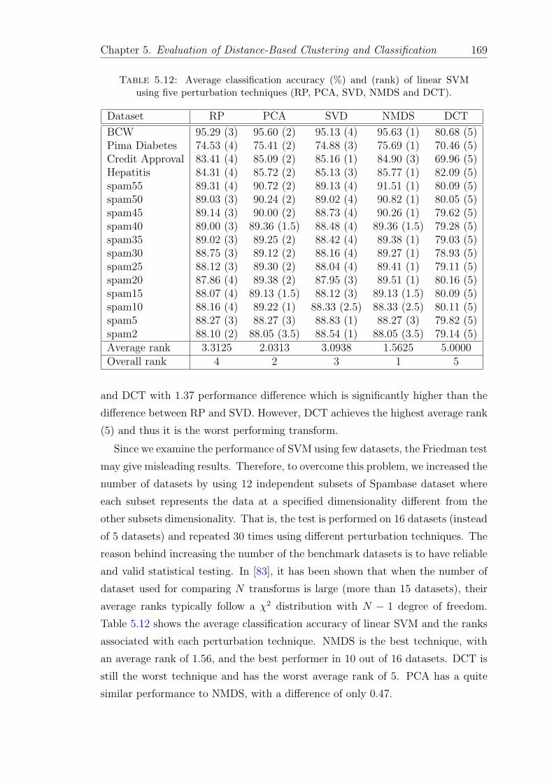
Chapter 5. Evaluation of Distance-Based Clustering and Classification 169
Table 5.12: Average classification accuracy (%) and (rank) of linear SVMusing five perturbation techniques (RP, PCA, SVD, NMDS and DCT).
Dataset RP PCA SVD NMDS DCT
BCW 95.29 (3) 95.60 (2) 95.13 (4) 95.63 (1) 80.68 (5)Pima Diabetes 74.53 (4) 75.41 (2) 74.88 (3) 75.69 (1) 70.46 (5)Credit Approval 83.41 (4) 85.09 (2) 85.16 (1) 84.90 (3) 69.96 (5)Hepatitis 84.31 (4) 85.72 (2) 85.13 (3) 85.77 (1) 82.09 (5)spam55 89.31 (4) 90.72 (2) 89.13 (4) 91.51 (1) 80.09 (5)spam50 89.03 (3) 90.24 (2) 89.02 (4) 90.82 (1) 80.05 (5)spam45 89.14 (3) 90.00 (2) 88.73 (4) 90.26 (1) 79.62 (5)spam40 89.00 (3) 89.36 (1.5) 88.48 (4) 89.36 (1.5) 79.28 (5)spam35 89.02 (3) 89.25 (2) 88.42 (4) 89.38 (1) 79.03 (5)spam30 88.75 (3) 89.12 (2) 88.16 (4) 89.27 (1) 78.93 (5)spam25 88.12 (3) 89.30 (2) 88.04 (4) 89.41 (1) 79.11 (5)spam20 87.86 (4) 89.38 (2) 87.95 (3) 89.51 (1) 80.16 (5)spam15 88.07 (4) 89.13 (1.5) 88.12 (3) 89.13 (1.5) 80.09 (5)spam10 88.16 (4) 89.22 (1) 88.33 (2.5) 88.33 (2.5) 80.11 (5)spam5 88.27 (3) 88.27 (3) 88.83 (1) 88.27 (3) 79.82 (5)spam2 88.10 (2) 88.05 (3.5) 88.54 (1) 88.05 (3.5) 79.14 (5)Average rank 3.3125 2.0313 3.0938 1.5625 5.0000Overall rank 4 2 3 1 5
and DCT with 1.37 performance difference which is significantly higher than the
difference between RP and SVD. However, DCT achieves the highest average rank
(5) and thus it is the worst performing transform.
Since we examine the performance of SVM using few datasets, the Friedman test
may give misleading results. Therefore, to overcome this problem, we increased the
number of datasets by using 12 independent subsets of Spambase dataset where
each subset represents the data at a specified dimensionality different from the
other subsets dimensionality. That is, the test is performed on 16 datasets (instead
of 5 datasets) and repeated 30 times using different perturbation techniques. The
reason behind increasing the number of the benchmark datasets is to have reliable
and valid statistical testing. In [83], it has been shown that when the number of
dataset used for comparing N transforms is large (more than 15 datasets), their
average ranks typically follow a χ2 distribution with N − 1 degree of freedom.
Table 5.12 shows the average classification accuracy of linear SVM and the ranks
associated with each perturbation technique. NMDS is the best technique, with
an average rank of 1.56, and the best performer in 10 out of 16 datasets. DCT is
still the worst technique and has the worst average rank of 5. PCA has a quite
similar performance to NMDS, with a difference of only 0.47.
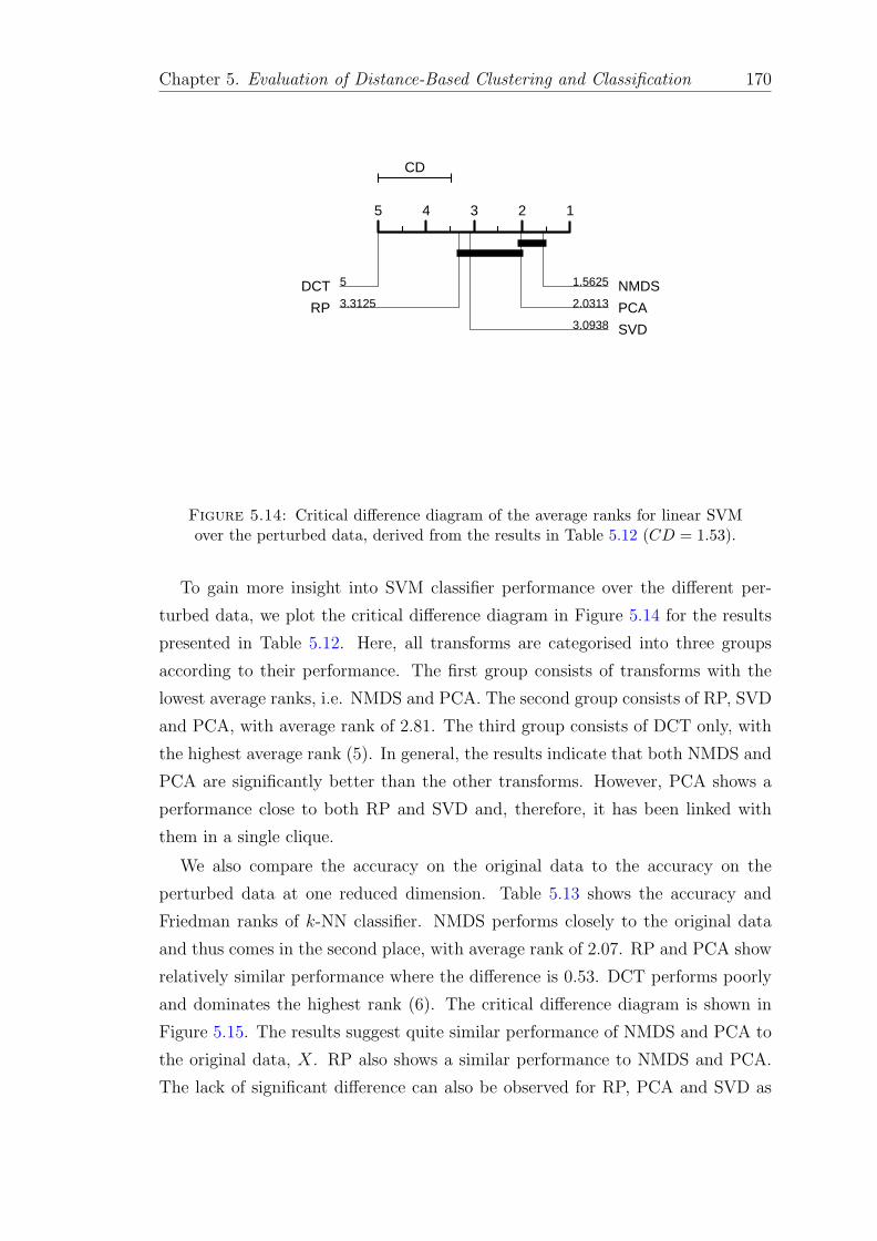
Chapter 5. Evaluation of Distance-Based Clustering and Classification 170
CD
5 4 3 2 1
1.5625 NMDS2.0313 PCA3.0938 SVD
3.3125RP
5DCT
Figure 5.14: Critical difference diagram of the average ranks for linear SVMover the perturbed data, derived from the results in Table 5.12 (CD = 1.53).
To gain more insight into SVM classifier performance over the different per-
turbed data, we plot the critical difference diagram in Figure 5.14 for the results
presented in Table 5.12. Here, all transforms are categorised into three groups
according to their performance. The first group consists of transforms with the
lowest average ranks, i.e. NMDS and PCA. The second group consists of RP, SVD
and PCA, with average rank of 2.81. The third group consists of DCT only, with
the highest average rank (5). In general, the results indicate that both NMDS and
PCA are significantly better than the other transforms. However, PCA shows a
performance close to both RP and SVD and, therefore, it has been linked with
them in a single clique.
We also compare the accuracy on the original data to the accuracy on the
perturbed data at one reduced dimension. Table 5.13 shows the accuracy and
Friedman ranks of k-NN classifier. NMDS performs closely to the original data
and thus comes in the second place, with average rank of 2.07. RP and PCA show
relatively similar performance where the difference is 0.53. DCT performs poorly
and dominates the highest rank (6). The critical difference diagram is shown in
Figure 5.15. The results suggest quite similar performance of NMDS and PCA to
the original data, X. RP also shows a similar performance to NMDS and PCA.
The lack of significant difference can also be observed for RP, PCA and SVD as

Chapter 5. Evaluation of Distance-Based Clustering and Classification 171
Table 5.13: Classification accuracy (%) and (rank) of k-NN at one reduceddimension.
Dataset X RP PCA SVD NMDS DCT
Wine 96.29 (1) 95.30 (3) 95.22 (4) 92.40 (5) 96.14 (2) 89.73 (6)BCW 96.11 (3) 96.06 (4) 96.48 (1) 95.21 (5) 96.30 (2) 95.06 (6)Iris 95.11 (1) 93.95 (4) 94.72 (3) 93.59 (5) 94.89 (2) 83.02 (6)HDigits 97.55 (1.5) 97.40 (4) 97.53 (3) 95.38 (5) 97.55 (1.5) 93.65(6)Ecoli 66.34 (1) 64.99 (5) 65.36 (4) 65.99 (2) 65.42 (3) 56.67(6)ImageSeg 94.01 (1.5) 93.85 (4) 93.91 (3) 93.33 (5) 94.01 (1.5) 91.33(6)MFeatures 96.37 (2.5) 96.04 (4) 96.66 (1) 93.73 (5) 96.37 (2.5) 90.73(6)PageBlocks 95.42 (1) 92.42 (4) 94.04 (3) 91.42 (5) 94.84 (2) 91.33(6)Spambase 91.36 (1.5) 91.36 (1.5) 91.23 (5) 91.31 (4) 91.34 (3) 85.12(6)Pima 73.89 (1) 72.67 (3) 72.15 (4) 72.00 (5) 73.29 (2) 70.55(6)Yeast 55.21 (1) 54.18 (3) 53.45 (4) 51.50 (5) 54.69 (2) 50.77(6)Satlog 88.44 (1) 88.21 (4) 88.23 (2.5) 86.64 (5) 88.23 (2.5) 84.64(6)SCC 97.93 (1) 97.44 (5) 97.70 (3) 97.67 (4) 97.88 (2) 91.44(6)Credit 83.96 (1) 83.42 (3) 83.25 (4) 82.57 (5) 83.71 (2) 80.40(6)Hepatitis 84.87 (4) 84.99 (3) 85.02 (2) 82.62 (5) 85.28 (1) 75.24(6)Ave. rank 1.53 3.63 3.10 4.67 2.07 6.00Overall 1 4 3 5 2 6
CD
6 5 4 3 2 1
1.5333 X2.0667 NMDS
3.1 PCA3.6333RP
4.6667SVD
6DCT
Figure 5.15: Critical difference diagram of the average ranks for k-NN classi-fier at one reduced dimension, n− 1, (CD = 1.98).
they are represented in a single clique. The worst performance is reported to SVD
and DCT with average ranks of 4.67 and 6, respectively.
Overall, the results reveal the good performance of NMDS in relation to the

Chapter 5. Evaluation of Distance-Based Clustering and Classification 172
other dimensionality reduction approaches in terms of retaining high data utility
for distance-based classification. The results also suggest some similarities between
NMDS and PCA, but NMDS is still the best performing technique as the accuracy,
in most cases, is the highest compared to the other approaches.
5.4 Summary
In this chapter, we benchmark our perturbation method against four alternative
perturbation techniques. We experiment with a variety of clustering and classifica-
tion algorithms and show that our method performs better than other dimension-
ality reduction techniques in terms of utility retained in the data. The patterns
inherited in the original data can easily be discovered in the perturbed data with
similar accuracies or even better in some cases.
The choice of which approach to use to perturb the data is crucial, but essen-
tially the perturbation method should not compromise either privacy or utility.
Although PCA provides very good data utility, it is vulnerable to some distance-
based privacy attacks since the location of the original data points can be estimated
when some prior knowledge is available to the attacker [108, 165]. RP, SVD and
DCT approaches cause more distortion to the data, and therefore, better privacy
would be achieved. However, the large size of distortion negatively affects the
utility of the data, and thus they seem inefficient, especially if the analysis utilises
the distance between data objects.
The main findings of this chapter are summarised as follows:
• For clustering, NMDS and PCA were the best and outperformed other tech-
niques. NMDS maintains better privacy against distance-based and PCA-
based attacks.
• Both NMDS and PCA demonstrate good neighbourhood preservation, good
class compactness and better class separation. The perturbed data gener-
ated using these methods are still good enough to provide for reasonable
discrimination between classes for SVM, and in some cases the data in the
lower dimensional spaces provide improved classification performance.
• The worse performance was reported for SVD and DCT due to the high
distortion they often cause to the original data.

Chapter 5. Evaluation of Distance-Based Clustering and Classification 173
• Using RP causes some distance distortion, specially at the low dimensions,
but, interestingly, the accuracy is highly competitive at the higher dimen-
sions.
• A trade-off between privacy and accuracy need to be determined so that the
data owner can choose an appropriate lower dimension and transform the
data to that dimension.

Chapter 6
Conclusions and Future Work
This thesis explored the geometric properties of non-metric MDS and its appli-
cation to data perturbation. The positive performance of non-metric MDS is a
consequence of the solid mathematical foundations it relies on, which ensure the
good preservation of distance and the versatility of concealing original data values.
The results of this study are promising and could contribute to an increased aware-
ness of privacy. The results could help data owners who decide to outsource their
data for data mining or share the analysis with other external parties. This chap-
ter summarises the work undertaken during this study and discusses the value and
limitations of our method for PPDM. It also recommends a number of areas that
could be investigated in the future to improve the performance of the proposed
method.
6.1 Conclusions
In this thesis, we considered the issue of protecting private information in
databases that are intended for outsourcing or sharing with other parties for the
purpose of distance-based analysis. Therefore, we have proposed a novel method
that is based on non-metric MDS for PPDM and implemented and tested it using
the capabilities of MATLAB.
The thesis can be summarised as follows. First, we surveyed the literature
to obtain useful insights and make a coherent categorisation of the most related
perturbation methods. Second, we introduced and discussed the main character-
istics of non-metric MDS and studied its capabilities in terms of data utility and
privacy. Third, we assessed both information loss and disclosure risks associated
with the proposed method under specific conditions and assumptions. Fourth, we
174

Chapter 6. Conclusions and Future Work 175
evaluated and tested the application of our method to data mining tasks, including
clustering and classification.
The term “privacy” in this work has different connotations than those for data
anonymisation [102, 113, 158], where reducing the risk of identifying individuals
is more important, and from differential privacy [54], which aims to ensure that
the presence or absence of any individual data has a statistically negligible effect
on the query results obtained by a predefined randomised function. Here, the
privacy concerns can distinctly be defined as whether or not the attacker is able
to estimate or reconstruct the original data values. This can also be extended to
include the ability to reverse-engineer the process of the transformation.
We have demonstrated that the non-metric MDS is a flexible perturbation
method that can be adapted to meet other information requirements and vari-
ous selection criteria. For instance, the pairwise distances can be calculated using
different distance metrics and the quality of the mapping can be assessed using
various measures. We have looked at the geometric properties underlying the
perturbed data and have shown their resistance to privacy threats. The overall
performance of the technique was evaluated and compared with some existing
techniques, and the results were very promising in confirming the suitability and
effectiveness of the proposed technique.
We have also shown the following in relation to non-metric MDS for data per-
turbation:
• Non-metric MDS often results in good correlation between the Euclidean
distance in the lower dimensional space and the dissimilarity in the higher
dimensional space. This means that the points in the perturbed data opti-
mally represent the objects in the original data, (i.e. the pairwise distances
are well preserved).
• The final solution is non-linearly derived by an unknown function (monotone
regression).
• The perturbed data are entirely independent from the original data, as we
only use the ordered dissimilarities to generate the final solution.
• The perturbed space, Y , generated by the non-metric MDS transformation,
T , is an ε-isometric space. This implies that the pairwise distances are
mapped with some small distortion, ε, which would effectively increase the
resistance to distance-based attacks.

Chapter 6. Conclusions and Future Work 176
• The perturbed data provide different statistics except the distance-related
statistics, which are preserved within a very small tolerance that will not
affect the accuracy of data mining model.
• It would be difficult (if not impossible) to recover or estimate the original
data values from the perturbed data due to the heavy distortion caused by
non-metric MDS.
We empirically examined the usefulness of the perturbed data for distance-based
data mining. We discovered that mapping the data into high dimensions, but
lower than the original dimensionality, results in the best trade-off performance.
The level of information loss, which is represented by the stress, confirms that
non-metric MDS perturbation successfully preserves data utility for data mining
tasks. The non-metric MDS provides a non-linear and smooth mapping of high-
dimensional input data into a low-dimensional space. The main characteristic of
the transformation provided by non-metric MDS is the preservation of the essential
topology of the original data. It has the ability to preserve the internal structure
in the input space by mapping nearby and far away points in the input space into
nearby and far away points, respectively, in the output space [90]. This feature
makes the perturbed data useful for distance-based data mining.
We also presented a theoretical study on evaluating privacy breaches when prior
knowledge is obtainable to the attacker. We proposed two privacy attacks and
quantitatively assessed the disclosure risk in the perturbed data. The first attack
is based on the non-linear least-squares technique, which attempts to minimise
the error of estimating the location of an unidentified point in the perturbed
data using some other known reference points. The second attack studies the
characteristics of the eigenvector space, which is generated by PCA and derived
from the known sample and the perturbed data, and attempts to find a closer
match to the eigenvector space of the original space so that the perturbed data
can be rotated along the best selected eigenvectors and the original data can be
recovered. The experimental results demonstrated the robustness and resistance
of non-metric MDS to these attacks because the perturbed data are subject to
high uncertainty and provide the attacker with less information about the original
data.
From a privacy-preserving perspective, non-metric MDS has distinguishing fea-
tures in comparison to existing perturbation techniques because it evades the as-
sumption made by these techniques that dissimilarities and distances are related

Chapter 6. Conclusions and Future Work 177
by some fixed formula. The solution generated by non-metric MDS introduces
further uncertainty because the dissimilarities are mapped into distances using a
non-metric function, (i.e. one that preserves the rank orders instead of the dis-
tances themselves). Since the actual distances between data objects are unknown,
it would be difficult for adversary attacks to breach privacy. Furthermore, non-
metric MDS does not use the variability of the data as a critical element in forming
the distances in the generated configuration; therefore, it avoids some of the strong
distributional assumptions that are necessary in variability-dependent techniques.
Although our study may have some limitations, we believe that our findings
are promising for better understanding of the issue of privacy in data mining ap-
plications. In general, non-metric MDS data perturbation has unique benefits for
PPDM. The patterns present in the original data can easily be discovered from
the perturbed data with similar or even better accuracy in some cases. Many
popular distance-based data mining algorithms are invariant to the perturbation.
For example, the classifiers, including nearest neighbour, linear SVM, and non-
linear SVM with kernel methods, trained on the perturbed data have almost the
same accuracy as those applied to the original data. This conclusion is also valid
for most popular distance-based clustering algorithms, including k-means, hier-
archical clustering, and density-based clustering. As described throughout this
thesis, retaining a large number of dimensions when perturbing the data obtains
the highest utility and may make the task of distance-based analysis easier. It is
also possible to apply data mining algorithms without having to modify them to
work with perturbed data.
In this thesis, we introduce the first use of a non-linear transformation, which is
represented by non-metric MDS, as a competitive method for data perturbation in
PPDM. Previous applications of non-metric MDS focused on visualisation [21, 30]
and pattern analysis [52]. To the best of our knowledge, this is the first study
to examine the suitability of non-metric MDS for PPDM. Non-metric MDS ad-
dresses problems that have been identified with previously proposed perturbation
methods, and when the results have been compared to those methods, non-metric
MDS has been found to be robust and competitive.
6.2 Limitations and Future Work
Some limitations of our work are worth mentioning, together with further work
necessary to extend the research, taking into account current limitations. These

Chapter 6. Conclusions and Future Work 178
include:
• Scalability of Non-metric MDS Algorithm
Due to the high computational complexity of the native non-metric MDS
algorithm, we use datasets with a relatively small number of data objects.
Obviously, we will need to work on making it scalable to large databases
in order for it to be used as more general perturbation tool for PPDM.
Scalability of the algorithm is left for future research.
• Uncertainty Quantification
Privacy quantification is an open research issue. In this work, we evaluate
privacy on the basis of the distance between the original and estimated data
using heuristic methods. However, other measures may be required and may
produce different understanding. For instance, it would be clever to use an
ad-hoc measure that indicates the uncertainty associated with the perturbed
data during the transformation process.
• Privacy Attacks
Another challenge in PPDM is modelling background knowledge that an
adversary obtains independently from other available data sources to conduct
privacy attacks. Clearly, it is difficult to provide a protection against attacks
with an arbitrarily large amount of knowledge because one may not be able
to predict which values of the original data may be inferred by the attacker
a priori. In our work, we consider two different attacks (Sections 4.4 and
4.5) based on an assumption that the attacker has some knowledge about
the original data. Then, we attempted to employ this information in our
simulated attacks in order to disclose the original data values. Nevertheless,
other attacks may be possible depending on different assumptions so we have
not comprehensively assessed every possible scenario. It may also be possible
to consider the problem of quantifying how much information is embedded
in the perturbed data and how the adversary could use this information to
attack the original data.
• Seeking The Best Mapping that Minimises Distortion
An essential task of distance-based data mining is that the object is assigned
to the right group according to a predefined distance function. Consequently,

Chapter 6. Conclusions and Future Work 179
preserving the distance-related properties of the underlying data in the low-
dimensional space provides high data utility and more accurate results would
be expected. This implies that whenever the stress is very small, the utility
is higher. As discussed in Section 4.2, the stress can be beneficially used to
reflect the goodness of the perturbed data for the analysis. However, it is
difficult to define a criterion that exactly determines a value of the stress in
which the derived solution represents the best representation of the original
data [18]. Thus, more systematic insight into how the stress depends on
the number of objects, dimensions, and errors in the dissimilarities would be
worth further investigation.
• The Choice of Distance Metric
Distance-based algorithms intend to group or classify a set of objects into
homogeneous non-overlapping subsets or groups according to some concept
of similarity, which is often expressed as some sort of distance between a pair
of objects. Therefore, the distance function should accurately reflect such
relationships in order to facilitate the task of the data mining algorithm.
In our work, this is also a limiting factor since our method only considers
the Euclidean distance (L2 norm) as a dissimilarity measure, which means
that it can only take into account the second-order statistics of the data. As
we have seen in Section 3.3.3, the distortion caused by non-metric MDS in
pairwise Euclidean distances is limited compared to other norms. However,
the effect of using other distance functions may be worth considering as
future work.
• Scenarios for PPDM
In our work, we have investigated two scenarios for PPDM: data outsourc-
ing and external access (Section 1.2). We believe that additional work on
distributed data analysis could be studied in conjunction with a variety of
distance-based data mining frameworks.
• Non-distance based data mining
Our privacy method attempts to generate data that preserve distance-related
properties. However, data mining algorithms vary according to the under-
lying properties they require during the learning process. For example, a
decision tree induction algorithm [160] recursively selects the best attribute

Chapter 6. Conclusions and Future Work 180
to split the data and expands the leaf nodes of the tree until a stopping crite-
rion is met. The choice of the best split is often determined by an information
gain ratio, which is based on the entropy metric. We have not investigated
how our perturbed data would work in the context of non-distance based
approaches. This could be attempted in further research.
• Other Potential Privacy Threats
Privacy concerns differ from one application to another and from one data
owner to another. However, it is essential, in both cases, that the privacy
should be defined clearly before publishing the data or sharing with external
parties. Many methods have been developed, each of which makes specific
assumptions to address the issue of privacy. For example, distribution es-
timation assumes that the perturbation is additive and the attacker knows
the distribution of the added noise, which is independent and identically
distributed. The attacker attempts to estimate the original distribution by
exploiting the properties of the random noise. Then, s/he can use the es-
timated distribution to train a decision-tree classifier and accurate results
may be obtained. Although this kind of attack may help, to some extent,
to estimate the original distribution, it is impossible to reconstruct the ex-
act distribution [5, 7]. If preventing the distribution estimation is a privacy
requirement of data owners, it would be better to consider this when design-
ing a privacy-preserving model. However, since our emphasis is initially on
providing much useful data for distance-based analysis, we defer the inves-
tigation of this problem to future work.

Appendix A
Triangle Geometry for
Non-Metric MDS
To illustrate how the points are placed in a configuration Y t where t is the itera-
tion’s number, assume that a, b, c are three data points in the data Y ; their inter-
point distances are dab, dbc and dac conforming to the rank-order dab ≤ dbc ≤ dac.
That is, these points form a triangle, as illustrated in Figure A.1(a). Assume that
the points a and c have been placed and that the distance between them is dac.
Without loss of generality, all possible positions for placing a point b, without
violating the constraint dab ≤ dbc ≤ dac, are bounded by the shaded area.
Similarly, consider another distances order: dab ≤ dac ≤ dbc. In this case, the
uncertainty about placing b will increase to include a wider area, as shown in
Figure A.1(b). The shaded area represents the uncertainty in placing the points,
which can prevent the attacker from exactly determining the position of any point.
In other words, point placement is governed by the rank-order of distances rather
than their real magnitudes.
To prove that the uncertainty of placing a given point is bounded by a closed
area in the mapping space, we have to introduce some elementary of triangle
geometry.
181
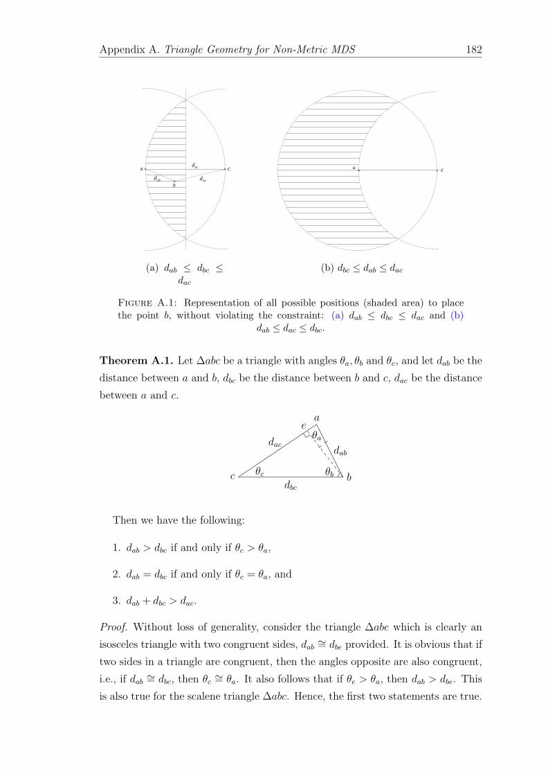
Appendix A. Triangle Geometry for Non-Metric MDS 182
x
x
xacd
bcdabd
c
b
a
(a) dab ≤ dbc ≤dac
x x ca
(b) dbc ≤ dab ≤ dac
Figure A.1: Representation of all possible positions (shaded area) to placethe point b, without violating the constraint: (a) dab ≤ dbc ≤ dac and (b)
dab ≤ dac ≤ dbc.
Theorem A.1. Let ∆abc be a triangle with angles θa, θb and θc, and let dab be the
distance between a and b, dbc be the distance between b and c, dac be the distance
between a and c.
c θcdbc
bθb
dab
a
θadac
e
Then we have the following:
1. dab > dbc if and only if θc > θa,
2. dab = dbc if and only if θc = θa, and
3. dab + dbc > dac.
Proof. Without loss of generality, consider the triangle ∆abe which is clearly an
isosceles triangle with two congruent sides, dab ∼= dbe provided. It is obvious that if
two sides in a triangle are congruent, then the angles opposite are also congruent,
i.e., if dab ∼= dbc, then θc ∼= θa. It also follows that if θe > θa, then dab > dbe. This
is also true for the scalene triangle ∆abc. Hence, the first two statements are true.
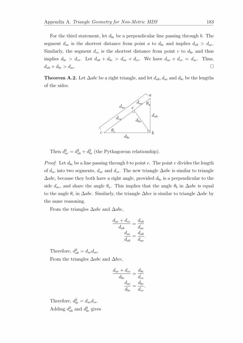
Appendix A. Triangle Geometry for Non-Metric MDS 183
For the third statement, let dbe be a perpendicular line passing through b. The
segment dae is the shortest distance from point a to dbe and implies dab > dae.
Similarly, the segment dce is the shortest distance from point c to dbe and thus
implies dbc > dce. Let dab + dbc > dae + dce. We have dae + dce = dac. Thus,
dab + dbc > dac.
Theorem A.2. Let ∆abc be a right triangle, and let dab, dac and dbc be the lengths
of the sides.
e
dbe
c θcdbc
b
dab
a
θa
dce
daedac
Then d2ac = d2
ab + d2bc (the Pythagorean relationship).
Proof. Let dbe be a line passing through b to point e. The point e divides the length
of dac into two segments, dae and dce. The new triangle ∆abe is similar to triangle
∆abc, because they both have a right angle, provided dbe is a perpendicular to the
side dac, and share the angle θa. This implies that the angle θb in ∆abe is equal
to the angle θc in ∆abc. Similarly, the triangle ∆bce is similar to triangle ∆abc by
the same reasoning.
From the triangles ∆abc and ∆abe,
dae + dcedab
=dabdae
dacdab
=dabdae
.
Therefore, d2ab = dacdae.
From the triangles ∆abc and ∆bce,
dae + dcedbc
=dbcdce
dacdbc
=dbcdce
.
Therefore, d2bc = dacdce.
Adding d2ab and d2
bc gives

Appendix A. Triangle Geometry for Non-Metric MDS 184
d2ab + d2
bc = dacdae + dacdce
= dac(dae + dce)
= dacdac.
Hence, d2ab + d2
bc = d2ac.
Definition A.3. Let ∆abc be a right triangle with an angle θb = 90◦, the acute
angles, θa and θc, are such that θc = cos−1(dbc
dac
)and θa = cos−1
(dab
dac
).
Given three ordered distances dab ≤ dbc ≤ dac, as in the previous example.
Assume that points a and c have been placed in their positions, and we want
to place a given point b, without violating the order condition. Figure A.2 shows
some three possible positions where point b is quite likely to be placed. Intuitively,
choosing any point bi in the shaded area satisfies the above condition. Now, let us
prove that point b will be somewhere within the shaded area.
Firstly, we check dac ≥ dbc. The distance dac is radius r, i.e., r = dac, and it
easy to see that
r = dac = db′c.
Now, we can see that db′c ≥ dbc. Thus,
r = dac > dbc.
Secondly, we check dbc ≥ dab. Consider the triangle in Figure A.2 whose vertices
are a, b′′ and c. It is clear that two sides are equal in length, dab′′ = db′′c, so that
by Theorem A.1,
θ1 = θ2,
and also,
θ2 + θ3 > θ1.
Hence,
dbc ≥ dab.
Similarly, we can show that changing the order would largely affect the place-
ment of a given point b, and thereby, increase the uncertainty of the location
where point b can be placed. Assume that we have distances with different order

Appendix A. Triangle Geometry for Non-Metric MDS 185
x
x
xr5.0r5.0
x
x
ca
''
ib
1
32
'
ibib
Figure A.2: Uncertainty boundary to place a point b under the constraintdab ≤ dbc ≤ dac.
dab ≤ dac ≤ dbc. Again, assume that points a and c have been placed and the
distance between them is the radius r of the circle whose centre is point a (in-
terchangeably point c) as shown in Figure A.3. Let A be the area where point b
can be place under the above condition, and B be the segment of the circle whose
centre is c. The area B can be calculated by the formula
B =1
2r2
(θ
180π − sin θ
),
so we need to find the angle θ. Since θ1 = θ2, the angle θ is
θ = θ1 + θ2 = 2θ1.
By theorem A.2
θ = 2 cos−1
( 12r
r
)= 2 cos−1
(1
2
)= 120◦.
So we have
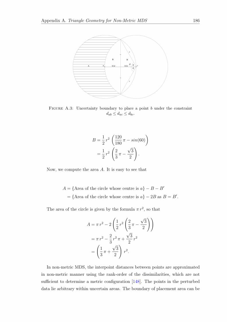
Appendix A. Triangle Geometry for Non-Metric MDS 186
x xr5.0r5.0 ca 1
2
r
r
'
θ
Figure A.3: Uncertainty boundary to place a point b under the constraintdab ≤ dac ≤ dbc.
B =1
2r2
(120
180π − sin(60)
)=
1
2r2
(2
3π −√
3
2
).
Now, we compute the area A. It is easy to see that
A = {Area of the circle whose centre is a} −B −B′
= {Area of the circle whose centre is a} − 2B as B = B′.
The area of the circle is given by the formula π r2, so that
A = π r2 − 2
(1
2r2
(2
3π −√
3
2
))
= π r2 − 2
3r2 π +
√3
2r2
=
(1
3π +
√3
2
)r2.
In non-metric MDS, the interpoint distances between points are approximated
in non-metric manner using the rank-order of the dissimilarities, which are not
sufficient to determine a metric configuration [148]. The points in the perturbed
data lie arbitrary within uncertain areas. The boundary of placement area can be

Appendix A. Triangle Geometry for Non-Metric MDS 187
small or large based on the corresponding order as shown earlier. Thus, the at-
tacker learns nothing from the perturbed data since they have no certain measures
that can be used to determine the exact positions of the points.

Bibliography
[1] S. Agarwal, J. Wills, L. Cayton, G. Lanckriet, D. J. Kriegman, and S. Be-
longie. Generalized non-metric multidimensional scaling. In International
Conference on Artificial Intelligence and Statistics, pages 11–18, 2007.
[2] C. Aggarwal and P. Yu. A General Survey of Privacy-Preserving Data Min-
ing Models and algorithms. In C. Aggarwal and P. Yu, editors, Privacy-
Preserving Data Mining: Models and Algorithms, chapter 2, pages 11 – 52.
Springer, 2008.
[3] C. C. Aggarwal, Y. Li, and P. S. Yu. On the hardness of graph anonymiza-
tion. In IEEE 11th International Conference on Data Mining (ICDM), pages
1002–1007. IEEE, 2011.
[4] C. C. Aggarwal and P. S. Yu. Outlier detection for high dimensional data.
In ACM Sigmod Record, volume 30, pages 37–46. ACM, 2001.
[5] D. Agrawal and C. C. Aggarwal. On the design and quantification of privacy
preserving data mining algorithms. In Proceedings of the twentieth ACM
SIGMOD-SIGACT-SIGART symposium on principles of database systems,
New York, USA, pages 247–255. ACM, 2001.
[6] R. Agrawal, C. Faloutsos, and A. Swami. Efficient similarity search in se-
quence databases. In D. B. Lomet, editor, Foundations of Data Organization
and Algorithms, Lecture Notes in Computer Science, pages 69–84. Springer,
Berlin, Heidelberg, 1993.
[7] R. Agrawal and R. Srikant. Privacy-preserving data mining. ACM Sigmod
Record, 29(2):439–450, 2000.
[8] S. Agrawal and J. R. Haritsa. A framework for high-accuracy privacy-
preserving mining. In Proceedings of the 21st International Conference on
Data Engineering (ICDE 2005), pages 193–204. IEEE, 2005.
188

Bibliography 189
[9] A. Ahmad and L. Dey. A k-mean clustering algorithm for mixed numeric
and categorical data. Data & Knowledge Engineering, 63(2):503–527, 2007.
[10] J. Bacardit and X. Llora. Large-scale data mining using genetics-based ma-
chine learning. Wiley Interdisciplinary Reviews: Data Mining and Knowl-
edge Discovery, 3(1):37–61, 2013.
[11] R. V. Banu and N. Nagaveni. Preservation of data privacy using PCA based
transformation. In Proceedings of the International Conference on Advances
in Recent Technologies in Communication and Computing (ARTCom’09),
pages 439–443. IEEE, 2009.
[12] V. Batagelj and M. Bren. Comparing resemblance measures. Journal of
classification, 12(1):73–90, 1995.
[13] R. J. Bayardo and R. Agrawal. Data Privacy through Optimal k-
Anonymization. In Proceedings of the 21st International Conference on Data
Engineering, pages 217–228. IEEE Computer Society, 2005.
[14] P. Berkhin. A survey of clustering data mining techniques. In Grouping
multidimensional data, pages 25–71. Springer, 2006.
[15] E. Bertino, D. Lin, and W. Jiang. A Survey of Quantification of Privacy
Preserving Data Mining Algorithms. In C. Aggarwal and P. Yu, editors,
Privacy-Preserving Data Mining: Models and Algorithms, chapter 8, pages
183–205. Springer, 2008.
[16] J. C. Bezdek, R. Ehrlich, and W. Full. Fcm: The fuzzy c-means clustering
algorithm. Computers & Geosciences, 10(2):191–203, 1984.
[17] C. M. Bishop and N. M. Nasrabadi. Pattern recognition and machine learn-
ing, volume 1. springer New York, 2006.
[18] I. Borg and P. J. F. Groenen. Modern multidimensional scaling: Theory and
applications. Springer Series in Statistics. Springer, 2005.
[19] R. N. Bracewell and R. Bracewell. The Fourier transform and its applica-
tions, volume 31999. McGraw-Hill New York, 1986.
[20] R. C. Brinker and R. Minnick. The Surveying Handbook. Chapman & Hall,
1995.

Bibliography 190
[21] A. Buja, D. F. Swayne, M. L. Littman, N. Dean, H. Hofmann, and L. Chen.
Data visualization with multidimensional scaling. Journal of Computational
and Graphical Statistics, 17(2):444–472, 2008.
[22] O. Chapelle, P. Haffner, and V. N. Vapnik. Support vector machines for
histogram-based image classification. Neural Networks, IEEE Transactions
on, 10(5):1055–1064, 1999.
[23] G. Chartrand, L. Eroh, M A Johnson, and Ortrud R Oellermann. Resolv-
ability in graphs and the metric dimension of a graph. Discrete Applied
Mathematics, 105(1):99–113, 2000.
[24] K. Chen and L. Liu. Privacy preserving data classification with rotation
perturbation. In Proceedings of the Fifth IEEE International Conference on
Data Mining, Houston, USA, pages 589–592, 2005.
[25] K. Chen and L. Liu. A survey of multiplicative perturbation for privacy-
preserving data mining. In C. Aggarwal and P. Yu, editors, Privacy-
Preserving Data Mining: Models and Algorithms, chapter 7, pages 157–181.
Springer, 2008.
[26] K. Chen and L. Liu. Privacy-preserving multiparty collaborative mining with
geometric data perturbation. IEEE Transactions on Parallel and Distributed
Systems, 20(12):1764–1776, 2009.
[27] K. Chen and L. Liu. Geometric data perturbation for privacy preserving
outsourced data mining. Knowledge and information systems, 29(3):657–
695, 2011.
[28] K. Chen, G. Sun, and L. Liu. Towards attack-resilient geometric data per-
turbation. In Proceedings of the Seventh SIAM Data Mining Conference,
Minneapolis, USA, pages 78–89. SDM’07, 2007.
[29] L. Chen and A. Buja. Local multidimensional scaling for nonlinear dimension
reduction, graph drawing, and proximity analysis. Journal of the American
Statistical Association, 104(485):209–219, 2009.
[30] L. Chen and A. Buja. Local multidimensional scaling for nonlinear dimension
reduction, graph drawing, and proximity analysis. Journal of the American
Statistical Association, 104(485):209–219, 2009.

Bibliography 191
[31] R. Chen, B. Fung, N. Mohammed, B. C. Desai, and K. Wang. Privacy-
preserving trajectory data publishing by local suppression. Information Sci-
ences, 231:83–97, 2013.
[32] C. Chow and M. F. Mokbel. Trajectory privacy in location-based services
and data publication. ACM SIGKDD Explorations Newsletter, 13(1):19–29,
2011.
[33] C. Clifton, M. Kantarcioglu, and J. Vaidya. Defining privacy for data mining.
In National science foundation workshop on next generation data mining,
pages 126–133, 2002.
[34] M. Collins, S. Dasgupta, and R. E. Schapire. A generalization of principal
component analysis to the exponential family. In Proceedings of the 14th
Annual Conference on Neural Information Processing Systems (NIPS), 2001.
[35] Federal Trade Commission. Choicepoint settles data security breach charges;
to pay $10 million in civil penalties, $5 million for consumer redress,
2006. http://www.ftc.gov/news-events/press-releases/2006/01/
choicepoint-settles-data-security-breach-charges-pay-10-million.
Retrieved: February 08, 2014.
[36] C. Cortes and V. Vapnik. Support-vector networks. Machine learning,
20(3):273–297, 1995.
[37] T. Cover and P. Hart. Nearest neighbor pattern classification. IEEE Trans-
actions on Information Theory, 13(1):21–27, 1967.
[38] T. M. Cover. Geometrical and statistical properties of systems of linear
inequalities with applications in pattern recognition. IEEE Transactions on
Electronic Computers, (3):326–334, 1965.
[39] T. M. Cover and J. A. Thomas. Elements of information theory. Wiley &
Sons, Inc., Hoboken, New Jersey, 2006.
[40] M.A.A. Cox and T.F. Cox. Multidimensional scaling. Handbook of data
visualization, pages 315–347, 2008.
[41] T. F. Cox and M. A. Cox. A general weighted two-way dissimilarity coeffi-
cient. Journal of Classification, 17(1):101–121, 2000.
Bibliography 192
[42] T. F. Cox and G. Ferry. Discriminant analysis using non-metric multidimen-
sional scaling. Pattern Recognition, 26(1):145–153, 1993.
[43] F. Critchley and B. Fichet. The partial order by inclusion of the principal
classes of dissimilarity on a finite set, and some of their basic properties. In
Classification and dissimilarity analysis, pages 5–65. Springer, 1994.
[44] D. R. Cutting, D. R. Karger, J. O. Pedersen, and J. W. Tukey. Scatter/-
gather: A cluster-based approach to browsing large document collections.
In Proceedings of the 15th annual international ACM SIGIR conference on
Research and development in information retrieval, pages 318–329. ACM,
1992.
[45] J. C. Debuse, B. de la Iglesia, C. M. Howard, and V. J. Rayward-Smith.
Building the KDD roadmap. In Industrial Knowledge Management, pages
179–196. Springer, 2001.
[46] J. Demsar. Statistical comparisons of classifiers over multiple data sets. The
Journal of Machine Learning Research, 7:1–30, 2006.
[47] M. M. Deza and E. Deza. Encyclopedia of distances. Springer, 2009.
[48] J. Domingo-Ferrer. A survey of inference control methods for privacy-
preserving data mining. In C. Aggarwal and P. Yu, editors, Privacy-
Preserving Data Mining: Models and Algorithms, chapter 3, pages 53–80.
Springer, 2008.
[49] J. Domingo-Ferrer and V. Torra. A critique of k-anonymity and some of its
enhancements. In Third International Conference on Availability, Reliability
and Security, ARES 08, pages 990–993. IEEE, 2008.
[50] J. Dricot, G. Bontempi, and P. Doncker. Static and dynamic localization
techniques for wireless sensor networks. In Sensor Networks, Signals and
Communication Technology, pages 249–281. Springer, 2009.
[51] H. Drucker, D. Wu, and V. N. Vapnik. Support vector machines for spam
categorization. IEEE Transactions on Neural Networks, 10(5):1048–1054,
1999.
[52] R. O. Duda, P. E. Hart, and D. G. Stork. Pattern Classification (2nd Edi-
tion). John Wiley & Sons, 2000.

Bibliography 193
[53] S. A. Dudani. The distance-weighted k-nearest-neighbor rule. Systems, Man
and Cybernetics, IEEE Transactions on, (4):325–327, 1976.
[54] C. Dwork. Differential privacy. In Proceedings of the 33rd International
Colloquium on Automata, Languages and Programming, Venice, Italy, pages
1–12. Springer, 2006.
[55] M. Ester, H. P. Kriegel, J. Sander, and X. Xu. A density-based algorithm for
discovering clusters in large spatial databases with noise. In Proceedings of
the 2nd International Conference on Knowledge Discovery and Data mining,
volume 1996, pages 226–231. AAAI Press, 1996.
[56] M. J. R. Fasham. A comparison of nonmetric multidimensional scaling, prin-
cipal components and reciprocal averaging for the ordination of simulated
coenoclines, and coenoplanes. Ecology, pages 551–561, 1977.
[57] U. Fayyad, G. Piatetsky-Shapiro, and P. Smyth. From data mining to knowl-
edge discovery in databases. AI magazine, 17(3):37, 1996.
[58] A. Frank and A. Asuncion. UCI machine learning repository, 2010. Univer-
sity of California, Irvine, School of Information and Computer Sciences.
[59] A. Friedman, R. Wolff, and A. Schuster. Providing k-anonymity in data
mining. The VLDB Journal, The International Journal on Very Large Data
Bases, 17(4):789–804, 2008.
[60] B. C. M. Fung, K. Wang, R. Chen, and P. S. Yu. Privacy-preserving data
publishing: A survey on recent developments. ACM Computing Surveys
(CSUR), 42(4):14:1–14:53, 2010.
[61] C. R. Giannella, K. Liu, and H. Kargupta. Breaching euclidean distance-
preserving data perturbation using few known inputs. Data & Knowledge
Engineering, 83:93–110, 2013.
[62] A. N. Gorban and A. Zinovyev. Principal manifolds and graphs in practice:
From molecular biology to dynamical systems. International Journal of
Neural Systems, 20(3):219–232, 2010.
[63] J. C. Gower. A general coefficient of similarity and some of its properties.
Biometrics, pages 857–871, 1971.

Bibliography 194
[64] J. C. Gower and P. Legendre. Metric and euclidean properties of dissimilarity
coefficients. Journal of classification, 3(1):5–48, 1986.
[65] S. Guo and X. Wu. On the use of spectral filtering for privacy preserving data
mining. In Proceedings of the 2006 ACM symposium on Applied computing,
Dijon, France, pages 622–626. ACM, 2006.
[66] S. Guo and X. Wu. Deriving private information from arbitrarily projected
data. Advances in Knowledge Discovery and Data Mining, pages 84–95,
2007.
[67] M. Halkidi, Y. Batistakis, and M. Vazirgiannis. On clustering validation
techniques. Journal of Intelligent Information Systems, 17(2):107–145, 2001.
[68] R. W. Hamming. Error detecting and error correcting codes. Bell System
technical journal, 29(2):147–160, 1950.
[69] J. Han, M. Kamber, and J. Pei. Data Mining: Concepts and Techniques.
Morgan Kaufmann Publishers Inc., San Francisco, CA, USA, 3rd edition,
2011.
[70] J. Handl, J. Knowles, and D. B. Kell. Computational cluster validation in
post-genomic data analysis. Bioinformatics, 21(15):3201–3212, 2005.
[71] F. Harary and R. A. Melter. On the metric dimension of a graph. Ars
Combinatoria, 2:191–195, 1976.
[72] J. R. Haritsa. Mining association rules under privacy constraints. In C. Ag-
garwal and P. Yu, editors, Privacy-Preserving Data Mining: Models and
Algorithms, chapter 10, pages 239–266. Springer, 2008.
[73] J. A. Hartigan and M. A. Wong. Algorithm as 136: A k-means cluster-
ing algorithm. Journal of the Royal Statistical Society. Series C (Applied
Statistics), 28(1):100–108, 1979.
[74] T. Hastie, R. Tibshirani, and J. Friedman. The elements of statistical learn-
ing, volume 1. Springer, New York, USA, 2001.
[75] X. He and P. Niyogi. Locality preserving projections. In S. Thrun, L. K.
Saul, and B. Scholkopf, editors, Advances in Neural Information Processing
Systems 16, pages 153–160. MIT Press, 2004.

Bibliography 195
[76] C. Hsu, C. Chang, and C. Lin. A practical guide to support vector classifica-
tion. Technical report, Department of Computer Science, National Taiwan
University, 2003.
[77] M. Hua and J. Pei. A survey of utility-based privacy-preserving data trans-
formation methods. In C. Aggarwal and P. Yu, editors, Privacy-Preserving
Data Mining: Models and Algorithms, chapter 9, pages 207–237. Springer,
2008.
[78] Z. Huang. Clustering large data sets with mixed numeric and categorical
values. In The First Pacific-Asia Conference on Knowledge Discovery and
Data Mining, pages 21–34. Citeseer, 1997.
[79] Z. Huang. Extensions to the k-means algorithm for clustering large data sets
with categorical values. Data Mining and Knowledge Discovery, 2(3):283–
304, 1998.
[80] Z. Huang, W. Du, and B. Chen. Deriving private information from ran-
domized data. In Proceedings of the 2005 ACM SIGMOD international
conference on Management of data, page 48. ACM, 2005.
[81] Z. Hubalek. Coefficients of association and similarity, based on binary
(presence-absence) data: An evaluation. Biological Reviews, 57(4):669–689,
1982.
[82] A. K. Jain, M. N. Murty, and P. J. Flynn. Data clustering: A review. ACM
computing surveys (CSUR), 31(3):264–323, 1999.
[83] N. Japkowicz and M. Shah. Evaluating Learning Algorithms. Cambridge
University Press, 2011.
[84] T. Joachims. Text categorization with support vector machines: Learning
with many relevant features. In Proceedings of the European Conference on
Machine Learning (ECML’98), pages 137–142, 1998.
[85] W. B. Johnson and J. Lindenstrauss. Extensions of Lipschitz mappings into
a Hilbert space. Contemporary mathematics, 26:189–206, 1984.
[86] I. T. Jolliffe. Principal Component Analysis (2nd Edition). Springer Verlag,
New York, 2002.

Bibliography 196
[87] M. Kantarcioglu. A survey of privacy-preserving methods across horizontally
partitioned data. In C. Aggarwal and P. Yu, editors, Privacy-Preserving
Data Mining: Models and Algorithms, chapter 13, pages 313–335. Springer,
2008.
[88] H. Kargupta, S. Datta, Q. Wang, and K. Sivakumar. On the Privacy Preserv-
ing Properties of Random Data Perturbation Techniques. In Proceedings of
the Third IEEE International Conference on Data Mining, Melbourne, USA,
pages 99–106. IEEE Computer Society, 2003.
[89] H. Kargupta, S. Datta, Q. Wang, and K. Sivakumar. Random-data per-
turbation techniques and privacy-preserving data mining. Knowledge and
Information Systems, 7(4):387–414, 2005.
[90] S. Katz, G. Leifman, and A. Tal. Mesh segmentation using feature point
and core extraction. The Visual Computer, 21(8-10):649–658, 2005.
[91] L. Kaufman and P. J. Rousseeuw. Finding groups in data: An introduction
to cluster analysis. John Wiley, New York, 1990.
[92] K. Kenthapadi, A. Korolova, I. Mironov, and N. Mishra. Privacy via the
johnson-lindenstrauss transform. Journal of Privacy and Confidentiality,
5(1):39–71, 2013.
[93] S. Khuller, B. Raghavachari, and A. Rosenfeld. Landmarks in graphs. Dis-
crete Applied Mathematics, 70(3):217–229, 1996.
[94] D. Kifer and J. Gehrke. Injecting utility into anonymized datasets. In
Proceedings of the 2006 ACM SIGMOD international conference on Man-
agement of data, page 228. ACM, 2006.
[95] J. J. Kim. A method for limiting disclosure in microdata based on random
noise and transformation. In Proceedings of the section on survey research
methods, pages 303–308, 1986.
[96] H. Kriegel, P. Kroger, M. Renz, and M. Schubert. Metric spaces in data
mining: applications to clustering. SIGSPATIAL Special, 2(2):36–39, 2010.
[97] J. B. Kruskal. Multidimensional scaling by optimizing goodness of fit to a
nonmetric hypothesis. Psychometrika, 29(1):1–27, 1964.
Bibliography 197
[98] J. B. Kruskal. Nonmetric multidimensional scaling: A numerical method.
Psychometrika, 29(2):115–129, 1964.
[99] M. N. Lakshmi and K. S. Rani. Privacy preserving clustering based on
singular value decomposition and geometric data perturbation. International
Journal of Computers & Technology, 10(3):1427–1433, 2013.
[100] J. A. Lee and M. Verleysen. Nonlinear dimensionality reduction. Springer,
2007.
[101] G. Li and Y. Wang. A privacy-preserving classification method based on
singular value decomposition. International Arab Journal of Information
Technology (IAJIT), 9(6), 2012.
[102] N. Li, T. Li, and S. Venkatasubramanian. t-Closeness: Privacy Beyond k-
Anonymity and l-Diversity. In Proceedings of the 23rd IEEE International
Conference on Data Engineering, Istanbul, Turkey, pages 106–115. IEEE,
2007.
[103] W. Li, S. Prasad, J. E. Fowler, and L. M. Bruce. Locality-preserving dis-
criminant analysis in kernel-induced feature spaces for hyperspectral image
classification. IEEE Geoscience and Remote Sensing Letters, 8(5):894–898,
2011.
[104] C. K. Liew, U. J. Choi, and C. J. Liew. A data distortion by probability
distribution. ACM Transactions on Database Systems (TODS), 10(3):395–
411, 1985.
[105] P. Lin, I. Jun Zhang, H. Wang, and J. Wang. A comparative study on
data perturbation with feature selection. In Proceedings of the International
MultiConference of Engineers and Computer Scientists, Hong Kong, pages
111–125, 2011.
[106] Y. Lindell and B. Pinkas. Secure multiparty computation for privacy-
preserving data mining. Journal of Privacy and Confidentiality, 1(1):59–98,
2009.
[107] K. Liu. Multiplicative Data Perturbation for Privacy Preserving Data Min-
ing. PhD thesis, University of Maryland, Baltimore County, Baltimore, MD,
2007.
Bibliography 198
[108] K. Liu, C. Giannella, and H. Kargupta. An attacker’s view of distance pre-
serving maps for privacy preserving data mining. In J. Frnkranz, T. Scheffer,
and M. Spiliopoulou, editors, Knowledge Discovery in Databases: PKDD
2006, volume 4213 of Lecture Notes in Computer Science, pages 297–308.
Springer, Berlin, Heidelberg, 2006.
[109] K. Liu, C. Giannella, and H. Kargupta. A survey of attack techniques on
privacy-preserving data perturbation methods. In C. Aggarwal and P. Yu,
editors, Privacy-Preserving Data Mining: Models and Algorithms, chap-
ter 15, pages 359–381. Springer, 2008.
[110] K. Liu, H. Kargupta, and J. Ryan. Random projection-based multiplicative
data perturbation for privacy preserving distributed data mining. IEEE
Transactions on Knowledge and Data Engineering, 18(1):92–106, 2006.
[111] L. Liu, K. Yang, L. Hu, and L. Li. Using noise addition method based on
pre-mining to protect healthcare privacy. Journal of Control Engineering
and Applied Informatics, 14(2):58–64, 2012.
[112] C. Ma, D. Yau, N. Yip, and N. Rao. Privacy vulnerability of pub-
lished anonymous mobility traces. IEEE/ACM Transactions on Networking,
21(3):720–733, 2013.
[113] A. Machanavajjhala, D. Kifer, J. Gehrke, and M. Venkitasubramaniam. `-
diversity: Privacy beyond k-anonymity. ACM Transactions on Knowledge
Discovery from Data (TKDD), 1(1):3, 2007.
[114] A. K. Maini and V. Agrawal. Satellite Technology: Principles and Applica-
tions. John Wiley & Sons, 2010.
[115] F. J. Massey. The kolmogorov-Smirnov test for goodness of fit. Journal of
the American statistical Association, 46(253):68–78, 1951.
[116] M. Meila. Comparing clusterings–an information based distance. Journal of
Multivariate Analysis, 98(5):873–895, 2007.
[117] B. Mendelson. Introduction to topology. Dover Publications, New York,
USA, 3nd edition, 1990.
[118] C. Meyer. Matrix analysis and applied linear algebra. Number 71. Society
for Industrial Mathematics, 2000.

Bibliography 199
[119] N. Mohammed, B. Fung, P. C. K. Hung, and C. Lee. Anonymizing healthcare
data: a case study on the blood transfusion service. In Proceedings of the
15th ACM SIGKDD international conference on Knowledge discovery and
data mining, pages 1285–1294. ACM, 2009.
[120] S. Mukherjee, M. Banerjee, Z. Chen, and A. Gangopadhyay. A privacy
preserving technique for distance-based classification with worst case privacy
guarantees. Data & Knowledge Engineering, 66(2):264–288, 2008.
[121] S. Mukherjee, Z. Chen, and A. Gangopadhyay. A privacy-preserving tech-
nique for Euclidean distance-based mining algorithms using Fourier-related
transforms. The International Journal on Very Large Data Bases, 15(4):293–
315, 2006.
[122] J. R. Munkres. Topology: A first course. Prentice-Hall, New Jersey, USA,
2nd edition, 2000.
[123] A. Narayanan and V. Shmatikov. Robust de-anonymization of large sparse
datasets. In IEEE Symposium on Security and Privacy, pages 111–125.
IEEE, 2008.
[124] W. Navidi, W. S. Murphy, and W. Hereman. Statistical methods in surveying
by trilateration. Computational statistics & data analysis, 27(2):209–227,
1998.
[125] R. T. Ng and J. Han. Efficient and effective clustering methods for spatial
data mining. In the 20th International Conference on Very Large Data Bases,
pages 144–155. Morgan Kaufmann Publishers Inc., San Francisco, CA, USA,
1994.
[126] The Office of Statewide Health Planning and Development. Inpatient data
reporting manual, 7th edition (10/13), 2013. http://www.oshpd.ca.gov/
hid/mircal/IPManual.html. Retrieved: February 08, 2014.
[127] E. Oja and A. Hyvarinen. Independent Component Analysis: Algorithms
and Applications. Neural Networks, 13(4-5):411–430, 2000.
[128] S. Oliveira and O. R. Zaıane. Privacy-preserving clustering by object
similarity-based representation and dimensionality reduction transforma-
tion. In Proceedings of the Workshop on Privacy and Security Aspects of

Bibliography 200
Data Mining (PSADM04) in conjunction with the Fourth IEEE Interna-
tional Conference on Data Mining (ICDM04), pages 21–30, 2004.
[129] S. Oliveira and O. R. Zaıane. Privacy-preserving clustering to uphold busi-
ness collaboration: A dimensionality reduction based transformation ap-
proach. International Journal of Information Security and Privacy, 1(2):13–
36, 2007.
[130] Executive Committee on ACMs SIGKDD. “Data Mining” is not against
civil liberties, 2003. Special Interest Group on Knowledge Discovery and
Data Mining. http://www.sigkdd.org/civil-liberties.pdf. Retrieved:
January 23, 2010.
[131] B. Pinkas. Cryptographic techniques for privacy-preserving data mining.
ACM SIGKDD Explorations Newsletter, 4(2):12–19, 2002.
[132] G. Pisier. The volume of convex bodies and Banach space geometry, vol-
ume 94. Cambridge University Press, 1999.
[133] J. O. Ramsay. Monotone regression splines in action. Statistical Science,
3(4):425–441, 1988.
[134] V. Rastogi, D. Suciu, and S. Hong. The boundary between privacy and utility
in data publishing. In Proceedings of the 33rd international conference on
Very large data bases, pages 531–542. VLDB Endowment, 2007.
[135] The Register. Acxiom database hacker jailed for 8 years, 2006. http:
//www.theregister.co.uk/2006/02/23/acxiom_spam_hack_sentencing.
Retrieved: February 08, 2014.
[136] R. Roscher, F. Schindler, and W. Frstner. High dimensional correspondences
from low dimensional manifolds—an empirical comparison of graph-based
dimensionality reduction algorithms. In R. Koch and F. Huang, editors,
Computer Vision ACCV 2010 Workshops, volume 6469 of Lecture Notes in
Computer Science, pages 334–343. Springer Berlin Heidelberg, 2011.
[137] S. T. Roweis and L. K. Saul. Nonlinear dimensionality reduction by locally
linear embedding. Science, 290(5500):2323–2326, 2000.
[138] W. Rudin. Principles of mathematical analysis. McGraw-Hill Book Co., New
York, 3rd edition, 1976. International Series in Pure and Applied Mathe-
matics.

Bibliography 201
[139] P. Samarati, S. Foresti, and V. Ciriani. k-anonymous data mining: A survey.
In C. Aggarwal and P. Yu, editors, Privacy-Preserving Data Mining: Models
and Algorithms, chapter 5, pages 105–136. Springer, 2008.
[140] J. W. Sammon. A nonlinear mapping for data structure analysis. IEEE
Transactions on Computers, 100(5):401–409, 1969.
[141] L. K. Saul, K. Q. Weinberger, J. H. Ham, F. Sha, and D. D. Lee. Spectral
methods for dimensionality reduction. Semi-Supervised Learning, pages 293–
308, 2006.
[142] A. Savvides, C. Han, and M. B. Strivastava. Dynamic fine-grained local-
ization in ad-hoc networks of sensors. In Proceedings of the 7th annual in-
ternational conference on Mobile computing and networking, MobiCom ’01,
Rome, Italy, pages 166–179. ACM, 2001.
[143] S. S. Schiffman, M. L. Reynolds, F. W. Young, and J. D. Carroll. In-
troduction to multidimensional scaling: Theory, methods, and applications.
Academic Press, New York, 1981.
[144] B. Scholkopf. The kernel trick for distances. Advances in neural information
processing systems, pages 301–307, 2001.
[145] D. W. Scott. Multivariate density estimation, volume 1. Wiley, New York,
USA, 1992.
[146] IBM Global Services. IBM Multi-national Consumer Privacy Sur-
vey, 1999. ftp://www6.software.ibm.com/software/security/privacy_
survey_oct991.pdf. Retrieved: February 21, 2010.
[147] H. Shatkay. The fourier transform-a primer. Technical report, Brown Uni-
versity, Providence, RI, USA, 1995.
[148] R. N. Shepard. The analysis of proximities: Multidimensional scaling with
an unknown distance function. II. Psychometrika, 27(3):219–246, 1962.
[149] R. N. Shepard. Metric structures in ordinal data. Journal of Mathematical
Psychology, 3(2):287–315, 1966.
[150] B. W. Silverman. Density estimation for statistics and data analysis, vol-
ume 26. Chapman & Hall, London, 1986.

Bibliography 202
[151] P. Y. Simard, Y. A. LeCun, J. S. Denker, and B. Victorri. Transformation
invariance in pattern recognition - tangent distance and tangent propagation.
In Neural networks: tricks of the trade, pages 239–274. Springer, 1998.
[152] L. I. Smith. A tutorial on principal components analysis. Technical report,
Cornell University, USA, 2002.
[153] I. Spence. A simple approximation for random rankings stress values. Mul-
tivariate Behavioral Research, 14(3):355–365, 1979.
[154] I. Spence and J. Graef. The determination of the underlying dimensionality
of an empirically obtained matrix of proximities. Multivariate Behavioral
Research, 9(3):331–341, 1974.
[155] I. Spence and J. C. Ogilvie. A table of expected stress values for random
rankings in nonmetric multidimensional scaling. Multivariate Behavioral
Research, 8(4):511–517, 1973.
[156] G. W. Stewart and J. Sun. Matrix perturbation theory. Academic Press,
New York, USA, 1990.
[157] G. Strang. Introduction to Linear Algebra. Wellesley-Cambridge Press, 4th
edition, 2009.
[158] L. Sweeney. k-anonymity: A model for protecting privacy. International
Journal of Uncertainty Fuzziness and Knowledge Based Systems, 10(5):557–
570, 2002.
[159] Y. Taguchi and Y. Oono. Relational patterns of gene expression via non-
metric multidimensional scaling analysis. Bioinformatics, 21(6):730–740,
2005.
[160] P. Tan, M. Steinbach, and V. Kumar. Introduction to data mining. Pearson
Addison Wesley, Boston, USA, 2006.
[161] J. B. Tenenbaum, V. De Silva, and J. C. Langford. A global geometric
framework for nonlinear dimensionality reduction. Science, 290(5500):2319–
2323, 2000.
[162] F. Thomas and L. Ros. Revisiting trilateration for robot localization. IEEE
Transactions on Robotics, 21(1):93–101, 2005.

Bibliography 203
[163] W. S. Torgerson. Multidimensional scaling: I. theory and method. Psy-
chometrika, 17(4):401–419, 1952.
[164] J. Traub, Y. Yemini, and H. Wozniakowski. The statistical security of
a statistical database. ACM Transactions on Database Systems (TODS),
9(4):672–679, 1984.
[165] E. Turgay, T. Pedersen, Y. Saygin, E. Savas, and A. Levi. Disclosure risks
of distance preserving data transformations. In Scientific and Statistical
Database Management, pages 79–94, Berlin, Heidelberg, 2008. Springer.
[166] J. K. Uhlmann. Satisfying general proximity/similarity queries with metric
trees. Information processing letters, 40(4):175–179, 1991.
[167] J. Vaidya. A survey of privacy-preserving methods across vertically parti-
tioned data. In C. Aggarwal and P. Yu, editors, Privacy-Preserving Data
Mining: Models and Algorithms, chapter 14, pages 337–358. Springer, 2008.
[168] J. Vaidya and C. Clifton. Privacy-preserving data mining: Why, how, and
when. IEEE Security & Privacy, 2(6):19–27, 2004.
[169] V. Vapnik. The nature of statistical learning theory. Springer, New York,
USA, 1995.
[170] V. Vapnik. The support vector method of function estimation. Nonlinear
Modeling: Advanced Black-Box Techniques, pages 55–85, 1998.
[171] J. Venna and S. Kaski. Neighborhood preservation in nonlinear projection
methods: An experimental study. Artificial Neural Networks-ICANN 2001,
pages 485–491, 2001.
[172] K. Veropoulos, C. Campbell, and N. Cristianini. Controlling the sensitiv-
ity of support vector machines. In Proceedings of the international joint
conference on artificial intelligence, pages 55–60, 1999.
[173] V. S. Verykios and P. Christen. Privacy-preserving record linkage. Wiley
Interdisciplinary Reviews: Data Mining and Knowledge Discovery, 3(5):321–
332, 2013.
[174] R. Vidya Banu and N. Nagaveni. Evaluation of a perturbation-based tech-
nique for privacy preservation in a multi-party clustering scenario. Informa-
tion Sciences, 232:437–448, 2013.

Bibliography 204
[175] J. T. Wang, X. Wang, K. Lin, D. Shasha, B. A. Shapiro, and K. Zhang.
Evaluating a class of distance-mapping algorithms for data mining and clus-
tering. In Proceedings of the fifth ACM SIGKDD international conference
on Knowledge discovery and data mining, pages 307–311. ACM, 1999.
[176] L. Wang, Y. Zhang, and J. Feng. On the euclidean distance of images. IEEE
Transactions on Pattern Analysis and Machine Intelligence, 27(8):1334–
1339, 2005.
[177] W. Wang, J. Yang, and R. Muntz. Sting: A statistical information grid
approach to spatial data mining. In the 23th International Conference on
Very Large Data Bases, volume 97, pages 186–195, 1997.
[178] S. Xu, J. Zhang, D. Han, and J. Wang. Singular value decomposition based
data distortion strategy for privacy protection. Knowledge and Information
Systems, 10(3):383–397, 2006.
[179] F. W. Young. Nonmetric multidimensional scaling: Recovery of metric in-
formation. Psychometrika, 35(4):455–473, 1970.
[180] F. W. Young. Quantitative analysis of qualitative data. Psychometrika,
46(4):357–388, 1981.
[181] F. W. Young. Scaling. Annual review of psychology, 35(1):55–81, 1984.


![Multi-Dimensional Transfer Function Design based on Flexible …hguo/publications/GuoXY11-small.pdf · Scaling (MDS) [35], which keeps the distance metric of the high dimensional](https://img.dokumen.tips/doc/110x75/5f04d5a77e708231d40ff15f/multi-dimensional-transfer-function-design-based-on-flexible-hguopublicationsguoxy11-smallpdf.jpg)