Non-Linear Regression Analysis · Residual plot in SPSS Research in Pharmacoepidemiology (RIPE) @ National School of Pharmacy, University of Otago. Residual plots in SPSS

Non-Linear Regression

AnalysisBy Chanaka Kaluarachchi

Research in Pharmacoepidemiology (RIPE) @ National School of Pharmacy, University of Otago

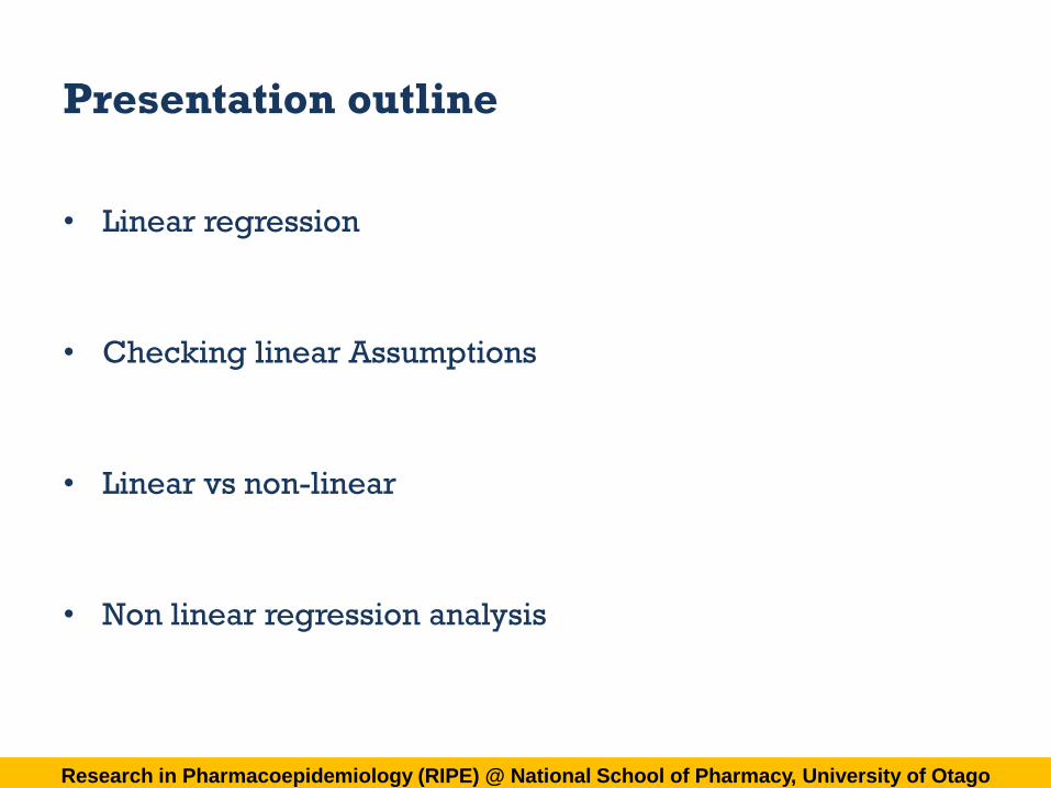
Presentation outline

• Linear regression

• Checking linear Assumptions

• Linear vs non-linear

• Non linear regression analysis


Linear regression (reminder)

• Linear regression is an approach for modelling dependent

variable(𝑦) and one or more explanatory variables (𝑥).

𝑦 = 𝛽0 + 𝛽1𝑥 + 𝜀

Assumptions:

𝜀~𝑁(0, 𝜎2 ) – iid ( independently identically distributed)


Checking linear Assumptions


iid- residual plot (𝜀 𝑣𝑠 𝑦) can be inspect to check that

assumptions are met.

• Constant variance- Scattering is a constant magnitude

• Normal data- few outliers, systematic spared above and

below the axis

• Liner relationship- No curve in the residual plot

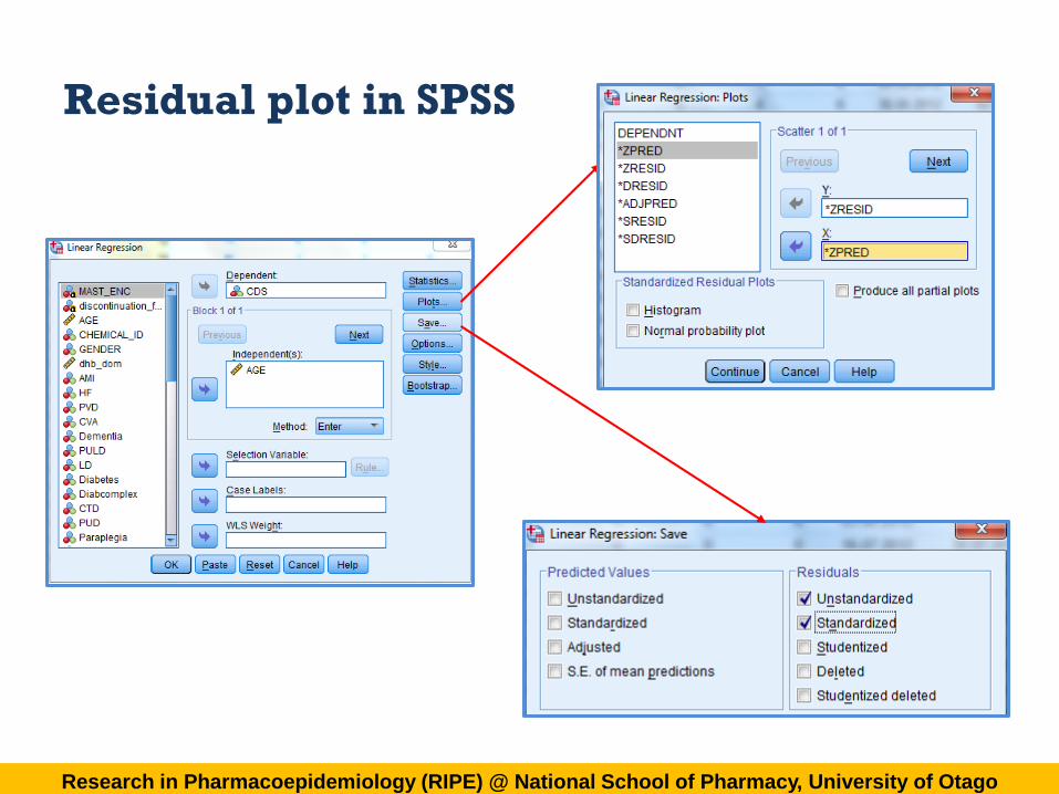
Residual plot in SPSS


Residual plots in SPSS


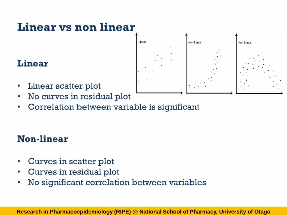
Linear vs non linear


Linear

• Linear scatter plot

• No curves in residual plot

• Correlation between variable is significant

Non-linear

• Curves in scatter plot

• Curves in residual plot

• No significant correlation between variables

Non linear regression


• Non linear regression arises when predictors and

response follows particular function form.

𝑦 = 𝑓 𝛽, 𝑥 + 𝜀

Examples

𝑦 = 𝛽2𝑥 + 𝜀 - non linear 𝑦 = 𝛽𝑥2 + 𝜀 - linear

𝑦 =1

𝛽𝑥 + 𝜀 - non linear 𝑦 = 𝛽

1

𝑥+ 𝜀 - linear

𝑦 = 𝑒𝛽𝑥 + 𝜀 - non linear 𝑦 = 𝛽 ln 𝑥 + 𝜀 - linear

𝑦 =1

1+𝛽𝑥+ 𝜀 - non linear

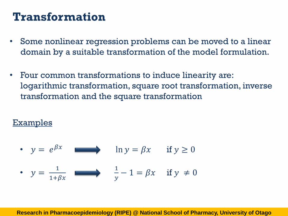
• Some nonlinear regression problems can be moved to a linear

domain by a suitable transformation of the model formulation.


Transformation

• Four common transformations to induce linearity are:

logarithmic transformation, square root transformation, inverse

transformation and the square transformation

Examples

• 𝑦 = 𝑒𝛽𝑥 ln 𝑦 = 𝛽𝑥 if 𝑦 ≥ 0

• 𝑦 =1

1+𝛽𝑥

1

𝑦− 1 = 𝛽𝑥 if 𝑦 ≠ 0


Curve Estimation

Curve fitting is the process of constructing a curve, or mathematical

function, that has the best fit to a series of data points.

Example –Viral growth model

• An internet service provider (ISP) is determining the effects of a

virus on its networks. As part of this effort, they have tracked the

(approximate) percentage of e-mail traffic on its networks over time,

from the moment of discovery until the threat was contained.


Curve Estimation- Cont.


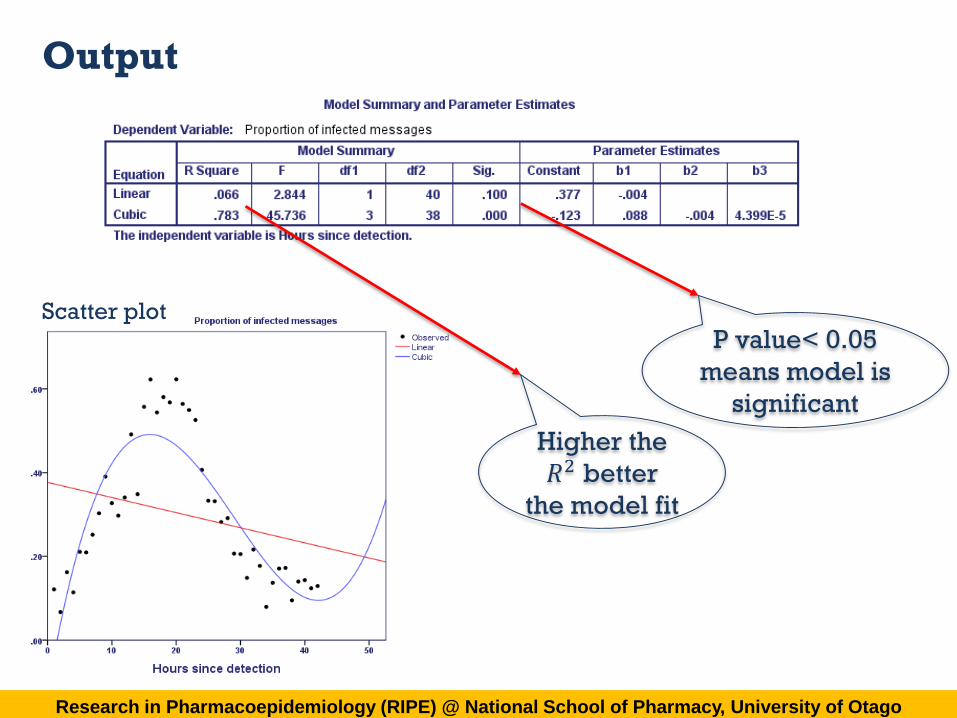
Output

Higher the

𝑅2 better

the model fit

P value< 0.05

means model is

significant

Scatter plot


Segmentation

We can split the graph in to segments and fit a segmented

model.

Example –Viral growth model

We can fit a logistic equation for the first 19 hours and an

asymptotic regression for the remaining hours should provide

a good fit and interpretability over the entire time period.


Logistic model and choosing starting values

𝑦 =𝛽1

1 + 𝛽2𝑒−𝛽3𝑥

Starting values

• 𝛽1- upper value of growth (0.65)

• 𝛽2- ratio upper value and lowest

value (0.65/0.13=5)

• 𝛽3- estimated slop between

points in plot.

(0.6-0.12/19-3)=0.03


Asymptotic regression model

𝑦 = 𝜃1 + 𝜃2𝑒𝜃3𝑥

Starting values

• 𝜃1- lowest value (0)

• 𝜃2- difference upper value and

lowest value (0.6)

• 𝛽3- estimated slop between

points in plot.

(0.6-0.1/20-40)=-0.025




Output


Output

Thanks for listening

Research in Pharmacoepidemiology (RIPE) @ National School of Pharmacy, University of OtagoResearch in Pharmacoepidemiology (RIPE) @ National School of Pharmacy, University of Otago

Documents

Non-Linear Regression Analysis · Residual plot in SPSS Research in Pharmacoepidemiology (RIPE) @ National School of Pharmacy, University of Otago. Residual plots in SPSS