Non-linear registration

aka

Spatial normalisation

FMRIB Technial Report TR07JA2

Jesper L. R. Andersson, Mark Jenkinson and Stephen Smith

FMRIB Centre, Oxford, United Kingdom

Correspondence and reprint requests should be sent to:

Jesper Andersson

FMRIB Centre

JR Hospital

Headington

Oxford OX3 9DU

phone: 44 1865 222 782

fax: 44 1865 222 717

mail: jesper@fmrib.ox.ac.uk

28 June 2007

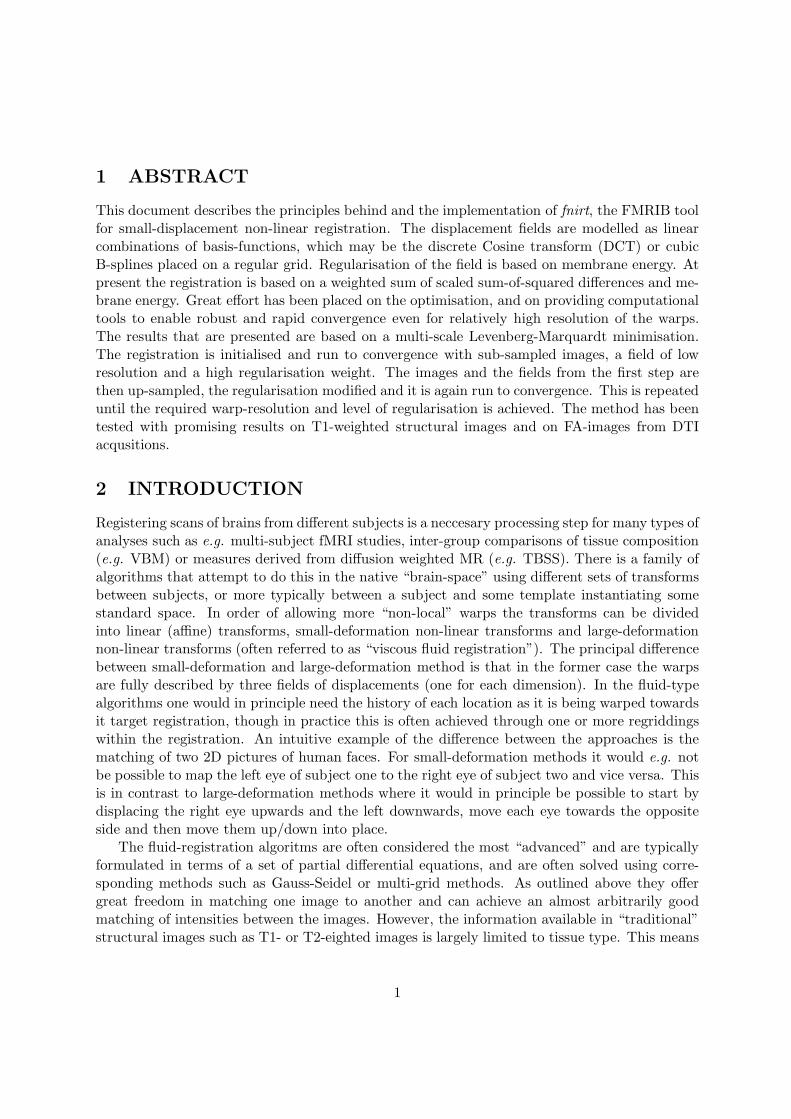
1 ABSTRACT

This document describes the principles behind and the implementation of fnirt, the FMRIB toolfor small-displacement non-linear registration. The displacement fields are modelled as linearcombinations of basis-functions, which may be the discrete Cosine transform (DCT) or cubicB-splines placed on a regular grid. Regularisation of the field is based on membrane energy. Atpresent the registration is based on a weighted sum of scaled sum-of-squared differences and me-brane energy. Great effort has been placed on the optimisation, and on providing computationaltools to enable robust and rapid convergence even for relatively high resolution of the warps.The results that are presented are based on a multi-scale Levenberg-Marquardt minimisation.The registration is initialised and run to convergence with sub-sampled images, a field of lowresolution and a high regularisation weight. The images and the fields from the first step arethen up-sampled, the regularisation modified and it is again run to convergence. This is repeateduntil the required warp-resolution and level of regularisation is achieved. The method has beentested with promising results on T1-weighted structural images and on FA-images from DTIacqusitions.

2 INTRODUCTION

Registering scans of brains from different subjects is a neccesary processing step for many types ofanalyses such as e.g. multi-subject fMRI studies, inter-group comparisons of tissue composition(e.g. VBM) or measures derived from diffusion weighted MR (e.g. TBSS). There is a family ofalgorithms that attempt to do this in the native “brain-space” using different sets of transformsbetween subjects, or more typically between a subject and some template instantiating somestandard space. In order of allowing more “non-local” warps the transforms can be dividedinto linear (affine) transforms, small-deformation non-linear transforms and large-deformationnon-linear transforms (often referred to as “viscous fluid registration”). The principal differencebetween small-deformation and large-deformation method is that in the former case the warpsare fully described by three fields of displacements (one for each dimension). In the fluid-typealgorithms one would in principle need the history of each location as it is being warped towardsit target registration, though in practice this is often achieved through one or more regriddingswithin the registration. An intuitive example of the difference between the approaches is thematching of two 2D pictures of human faces. For small-deformation methods it would e.g. notbe possible to map the left eye of subject one to the right eye of subject two and vice versa. Thisis in contrast to large-deformation methods where it would in principle be possible to start bydisplacing the right eye upwards and the left downwards, move each eye towards the oppositeside and then move them up/down into place.

The fluid-registration algoritms are often considered the most “advanced” and are typicallyformulated in terms of a set of partial differential equations, and are often solved using corre-sponding methods such as Gauss-Seidel or multi-grid methods. As outlined above they offergreat freedom in matching one image to another and can achieve an almost arbitrarily goodmatching of intensities between the images. However, the information available in “traditional”structural images such as T1- or T2-eighted images is largely limited to tissue type. This means

1

that prety much any mapping between two images that map gray matter onto gray matter,white matter onto white matter and CSF onto CSF is equally good in terms of the cost-functionand the task of finding the “true” warps can be thought of as finding the most likely set of warpsof those that yield that best cost-function value. It can therefore be argued that warps froma small-deformation model that yields a similar or identical cost-function value as those froma large-deformation model represents a more “reasonable” solution to the registration problem.Furthermore, it is clear that there exist no one-to-one mapping as defined by gyri and sulcibetween different brains. There is a set of sulci that are consistently found across “normal”subjects such as e.g. the interhemispheric fissure, the Sylvian fissure, the parietal-occipital fis-sure and the central sulcus. In contrast there appear to be large inter-subject differences ine.g. parietal cortex where it has been reported that not even the number of sulci is consistentacross “normal” subjects. Even though it would seem reasonable to assume that there exist atleast a functional one-to-one mapping across subjects there is insufficient experimental data toconclude even that. Indeed there exists studies which indicate that even low-level tasks such ase.g. odd-ball detection is processed differently in different subjects.

In this work we have therefore opted for a small-deformation model for the warps, and put ourefforts into ensuring convergence to a plausible field. We have aimed at achieveing that througha combination of a pyramid, or multi-resolution, scheme along with an afficient optimisationalgorithm for each step of the pyramid.

3 THEORY

3.1 Transforms and some definitions

The general transform of coordinates for nonlinear registration is of the form

x′

y′

z′

1

= M

xyz1

+

dx(x, y, z)dy(x, y, z)dz(x, y, z)

1

(1)

where M is an affine transform matrix that will account for differences in voxel-size, position,etc. For the reminder of this paper we will assume that M is known. The entities di(x, y, z) areknowns as displacement fields, and will for each location [x y z] tell how far the sampling pointshould be displaced in the i direction.

We will further assume the existence of some interpolating function such that given samplesof some function g(i, j, k) where i, j and k are sampled on some regular grid we can infer valuesg(x, y, z) as long as x, y and z fall within the original grid. We will then use g(x′, y′, z′) to denotethe values of g for a set of coordinates given by 1. This value can be thought of as the value ofg at some point [x y z] under the transform given by M and the displacement fields di(x, y, z).

In this paper we will use basis-functions to model the fields di(x, y, z) as a function of someset of parameters w. We can for example model the field as a linear combination of 3D cubicB-splines. Each spline in the 3D set is associated with a spline coordinate lmn specifying theposition of the spline in the space given by xyz. We will use Blmn(x, y, z) to denote the value ofthe spline with coordinate lmn at the location [x y z]. Each of these splines are then multipled

2

by a coefficient clmn, specifying how much is needed of that particular spline (see fig. ?). Wenow vectorise the coefficients clmn and denote the resulting vector by wi where i denotes thedirection of the field such that e.g. wx denotes the vector containing the coefficients definingthe dx(x, y, z) displacement field. Furthermore we denote the concatenation of these vectors byw, i.e w = [w(x)T w(y)T w(z)T ]T . With this notation we can the write gxyz(w) to denote thevalue of g at [x′ y′ z′] under the transform given by w implicit on the (constant) M.

The general notation gxyz(w) is independent of our choice of basis-function and would beequally valid for e.g a discrete cosine basis set.

We will also make use of the gradient, or rather its components, of g at some point [x′ y′ z′],which we define as

∇gxyz(w) =[

∂gxyz

∂x

∣∣∣w

∂gxyz

∂z

∣∣∣w

∂gxyz

∂z

∣∣∣w

]

(2)

where the partial derivative with respect to e.g x, ∂gxyz/∂x|w, denotes the rate of change ofg at [x′ y′ z′] as one translates the sampling point in the x-direction. It should be noted thatthe exact form of the partial derivatives ∂g/∂x is conditional on the interpolating function al-luded to above. In the present paper we will ignore this issue and assume the existence offunctions/kernels to perform the interpolation and calculating the corresponding partial deriva-

tives. If we now assume that the parameter w(x)i is the coefficient for the lmnth spline in the

x-displacement field dx we can denote the derivative of g as

∂gxyz

∂w(x)i

∣∣∣∣∣w

=∂gxyz

∂x

∣∣∣∣w

Blmn(x, y, z) (3)

where the w subscript indicates that is has been calculated at a point w in the parameter space.Let us further define the vector

g(w) =

g111(w)g211(w)gX11(w)

...g121(w)g221(w)

...gX21(w)

...gXY 1(w)

...gXY Z(w)

(4)

where x, y and z are defined on the ranges 1–X, 1–Y and 1–Z respectively. In an equivalent

3

manner we define the vectors

∂g

∂x

∣∣∣∣w

=

∂g111

∂x

∣∣∣w

∂g211

∂x

∣∣∣w

...∂gXY Z

∂x

∣∣∣w

(5)

and

Blmn =

Blmn(1, 1, 1)Blmn(2, 1, 1)

...Blmn(X,Y,Z)

(6)

Noting that there is a direct mapping from the index i into w to the triplet lmn we can equallywell, and more succinctly, write Bi as Blmn for the vector representation of the ith basis function.Combining equations 3, 5 and 6 we can further define the matrix

Jx(w) =[

∂g

∂x

∣∣∣w�B1

∂g

∂x

∣∣∣w� B2 . . . ∂g

∂x

∣∣∣w� BLMN

]

(7)

where � denotes elementwise (or Hadamard) product. Hopefully it should be clear that eachelement of Jx(w) is of the form given by equation 3. Finally by thinking of g(w) as an <3LMN →<XY Z mapping where L, M and N are the number of basis-functions and X, Y and Z are thenumber of samples/voxels in the x-, y- and z-directions respectively we can define the Jacobianmatrix J of that mapping as

J(w) =[

Jx(w) Jy(w) Jz(w)]

︸ ︷︷ ︸

XY Z×3LMN

(8)

3.2 Sum of squared differences cost-function

Our task is to find the parameters w describing the fields di(x, y, z) that transforms our func-tion/image g from its native space to some other arbitrary reference space. In this paperwe consider intensity-based methods for finding these. This is performed by defining somecost/objective-function in terms of some template f that defines our reference space and our ob-ject image g(w). Let us call this function O, and let us write it as O(w) as a short for O(f ,g(w)).An example of such a function is the “mean sum of squared differences” cost-function which wecan write as

O(w) =1

XY Z

Z∑

z=1

Y∑

y=1

X∑

x=1

(gxyz(w) − fxyz)2 (9)

or equivalently using the notation we defined in equation 4

O(w) =1

XY Z(g(w) − f)T (g(w) − f) (10)

4

In this case O is indeed a cost-function, i.e the smaller it is the happier we are. The generalstrategy of finding an estimate w is then to find

minarg w

O(w) (11)

3.3 What do we need for minimising the cost-function

Apart from time and patience, that is. Methods for minimsation of functions that are non-linearin the parameters of interest come in various flavors. Some rely solely on the ability to calculatethe costfuntion O at any point w in the parameter space. These methods typically need tocalculate O at a large number of points are are therefore not practical for problems where w

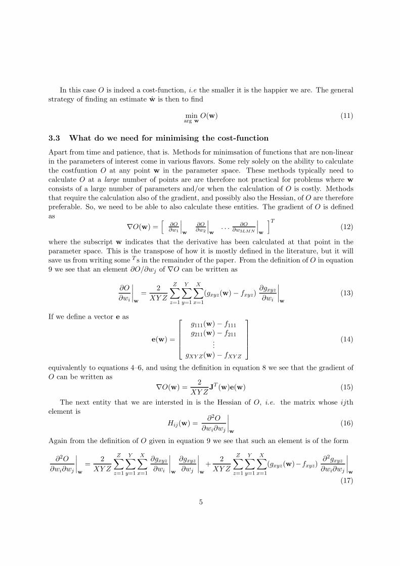
consists of a large number of parameters and/or when the calculation of O is costly. Methodsthat require the calculation also of the gradient, and possibly also the Hessian, of O are thereforepreferable. So, we need to be able to also calculate these entities. The gradient of O is definedas

∇O(w) =[

∂O∂w1

∣∣∣w

∂O∂w2

∣∣∣w

. . . ∂O∂w3LMN

∣∣∣w

]T

(12)

where the subscript w indicates that the derivative has been calculated at that point in theparameter space. This is the transpose of how it is mostly defined in the literature, but it willsave us from writing some T s in the remainder of the paper. From the definition of O in equation9 we see that an element ∂O/∂wj of ∇O can be written as

∂O

∂wi

∣∣∣∣w

=2

XY Z

Z∑

z=1

Y∑

y=1

X∑

x=1

(gxyz(w) − fxyz)∂gxyz

∂wi

∣∣∣∣w

(13)

If we define a vector e as

e(w) =

g111(w) − f111

g211(w) − f211...

gXY Z(w) − fXY Z

(14)

equivalently to equations 4–6, and using the definition in equation 8 we see that the gradient ofO can be written as

∇O(w) =2

XY ZJT (w)e(w) (15)

The next entity that we are intersted in is the Hessian of O, i.e. the matrix whose ijthelement is

Hij(w) =∂2O

∂wi∂wj

∣∣∣∣w

(16)

Again from the definition of O given in equation 9 we see that such an element is of the form

∂2O

∂wi∂wj

∣∣∣∣w

=2

XY Z

Z∑

z=1

Y∑

y=1

X∑

x=1

∂gxyz

∂wi

∣∣∣∣w

∂gxyz

∂wj

∣∣∣∣w

+2

XY Z

Z∑

z=1

Y∑

y=1

X∑

x=1

(gxyz(w)−fxyz)∂2gxyz

∂wi∂wj

∣∣∣∣w

(17)

5

Using equations 8 and 17 we see that we can write the Hessian matrix H as

H(w) =2

XY ZJT (w)J(w) + term with weird second derivatives (18)

The first term in equation 18 is known as the Gauss-Newton approximation to the Hessian. Inour technical report on optimisation we explain why this works, and often works better than ifusing the exact Hessian. For the remainder of this paper we will work with an approximationof the hessian given by

H(w) ≈2

XY ZJT (w)J(w) (19)

3.3.1 Relation to my code

In the implementation of fnirt there is a virtual base class called basisfield from which twoclasses, splinefield and dctfield, have been derived. An object of such a class containsinformation about the field it implements. So if we were to e.g to declare a field of typesplinefield we would do it like

std::vector<int> field_size(3), knot_spacing(3);

field_size[0] = 128; field_size[1] = 128; field_size[2] = 96;

knot_spacing[0] = 8; knot_spacing[1] = 8; knot_spacing[1] = 8;

BASISFIELD::splinefield xfield(field_size,knot_spacing);

Thus we have an object called xfield, corresponding to the entity dx(x, y, z) in the textabove, implementing a cubic B-spline field of size 128 × 128 × 96, corresponding to X × Y × Zin the equations above, with a knot-spacing of 8 voxels. The latter means that the splines areplaced on a regular grid with a distance of 8 voxels between adjacent spline kernels. These areplaced such that the centre of spline # 2 coincides with the centre of the first voxel and thenplaced at regular intervals of 8 voxels until the first kernel whose whole support falls outside thefield. From this are given the entities L, M and N in the equations above, and we can enquireabout these of our field as

int L = xfield.CoefSz_x();

int M = xfield.CoefSz_y();

int N = xfield.CoefSz_z();

Let us now say we have vectors f, g, and dgdx containing the reference image f , the objectimage g and the partial derivative w.r.t. x, ∂g/∂x, both sampled at some point w in referencespace. And let us say the we now want to calculate the gradient and Hessian of O. We can thennote that

∇O(w) =2

XY ZJT (w)e(w) =

2

XY Z

JTx (w)e(w)

JTy (w)e(w)

JTz (w)e(w)

(20)

Thus we can calculate the upper third of ∇O from

NEWMAT::ColumnVector f(xfield.FieldSz()), g(xfield.FieldSz()), dgdx(xfield.FieldSz());

... /* Use NEWIMAGE to calculate values for f, g and dgdx */

6

NEWMAT::ColumnVector e = g-f;

NEWMAT::ColumnVector nablaO(3*xfield.CoefSz());

nablaO.Rows(1,xfield.CoefSz()) = (2.0/xfield.FieldSz()) * xfield.Jte(dgdx,e);

We want of course all of nablaO and we would get that from corresponding field objects fordy(x, y, z) and dz(x, y, z)

NEWMAT::ColumnVector f(xfield.FieldSz());

NEWMAT::ColumnVector g(f), dgdx(f), dgdy(f), dgdz(f);

... /* Use NEWIMAGE to calculate values for f, g, dgdx, dgdy and dgdz */

NEWMAT::ColumnVector e = g-f;

int cfsz = xfield.CoefSz();

NEWMAT::ColumnVector nablaO(3*cfsz);

nablaO.Rows(1,cfsz) = (2.0/xfield.FieldSz()) * xfield.Jte(dgdx,e);

nablaO.Rows(cfsz+1,2*cfsz) = (2.0/yfield.FieldSz()) * yfield.Jte(dgdy,e);

nablaO.Rows(2*cfsz+1,3*cfsz) = (2.0/zfield.FieldSz()) * zfield.Jte(dgdz,e);

In the code above we could actually make do with a single field, provided we want to modelthe x-, y- and z-displacement fields with the same resolution, which we assume we always want.The important thing in the example above is that the member function Jte gets called withdifferent partial derivatives. However, in any actual case we will still need to represent the threedisplacement fields.

The next entity we would like to calculate is the (approximate) Hessian of O. Looking atequations 8 and 19 we see that it can be written as

H(w) ≈2

XY ZJT (w)JT (w) =

2

XY Z

JTx (w)JT

x (w) JTx (w)JT

y (w) JTx (w)JT

z (w)

JTy (w)JT

x (w) JTy (w)JT

y (w) JTy (w)JT

z (w)

JTz (w)JT

x (w) JTz (w)JT

y (w) JTz (w)JT

z (w)

(21)

Let us now look at how we would calculate two of the submatrices, JTx (w)Jx(w) and JT

x (w)Jy(w).

BASISFIELD::splinefield xfield(field_size,knot_spacing);

NEWMAT:ColumnVector dgdx(xfield.CoefSz()), dgdy(xfield.CoefSz());

... /* Use NEWIMAGE to calculate dgdx and dgdy */

boost::shared_ptr<MISCMATHS::BFMatrix> Hxx = xfield.JtJ(dgdx);

Hxx->MulMeByScalar(2.0/xfield.FieldSz());

boost::shared_ptr<MISCMATHS::BFMatrix> Hxy = xfield.JtJ(dgdy,dgdx);

Hxy->MulMeByScalar(2.0/xfield.FieldSz());

Please don’t be confused by the declaration of Hxx and Hxy. It is basically a pointer toan object of type BFMatrix. The class BFMatrix in turn is a virual base class with two de-rived classes SparseBFMatrix and FullBFMatrix which implements interfaces to sparse and fullmatrices respectively.

The final thing that should be pointed out in this section is that it is very easy to write codethat is independent of what basis-set we actually want to use. The following code would forexample work

7

boost::shared_ptr<basisfield> myfield;

if (I_like_splines == true) {myfield = boost::shared_ptr<splinefield>(new splinefield(fsize,ksp));

}else {myfield = boost::shared_ptr<dctfield>(new dctfield(fsize,order));

}

ColumnVector nablaO = myfield->Jte(dgdx,e);

nablaO &= myfield->Jte(dgdy,e);

nablaO &= myfield->Jte(dgdz,e);

nablaO *= 2.0/myfield.FieldSz();

boost::shared_ptr<BFMatrix> = myfield->JtJ(dgdx);

etc etc

So, you can see that after the initial creation of the field we can do all we need to do withit without actually having to know what type of field it is.

3.4 Sum of squared differences cost-function with scaling

This is a tiny change compared to the “sum of squared differences” described above. But itis of interest because it is the first (most basic) actual cost-function implemented in fnirt, andas such will allow us further insights into the structure of the code. For the more generalcases later on it is now useful to define the vector θ as the concatenation of w, the parameterspertaining to the displacement field, and any other parameters we might want to introduce.These other parameters will typically be used to model variations/differences in intensity thatdoes not pertain to structure and can hence be seen as confounds within the present problem.The very simplest form would be a scalar scaling factor that models global intensity differencesbetween f and g. So, let us now define θ as

θ =

[w

α

]

(22)

and the cost-function as

O(θ) =1

XY Z

Z∑

z=1

Y∑

y=1

X∑

x=1

(gxyz(w) − αfxyz)2 (23)

or

O(θ) =1

XY Z(g(w) − αf)T (g(w) − αf) (24)

which yields the gradient

∇O(θ) =2

XY Z

[JT (w)(g(w) − αf)−fT (g(w) − αf)

]

(25)

and the (approximate) Hessian

H(θ) =2

XY Z

[JT (w)J(w) −JT (w)f−fTJ(w) fT fT

]

(26)

8

3.4.1 So, how do we calculate that using the basisfield class?

The upper left block is identical to before, so we have already seen how to calculate that. It canfurther be seen that the block consisting of −JT (w)f is of the same general form as the upperportion of the gradient, only with the vector (g(w) − αf) replaced by f .

splinefield xfield(fsize,ksp), yfield(fsize,ksp), ...

ColumnVector f, g, e, dgdx, dgdy, dgdz;

.../* Calculate g, e, dgdx etc */

ColumnVector nablaO = xfield.Jte(dgdx,e) & xfield.Jte(dgdy,e) & xfield.Jte(dgdz,e);

nablaO &= DotProduct(f,e);

nablaO *= (2.0/xfield.FieldSz());

boost::shared_ptr<BFMatrix> JtJ;

.../* Calculate the 9 components of JtJ, and put them together */

ColumnVector toprightbit = xfield.Jte(dgdx,f) & xfield.Jte(dgdy,f) & xfield.Jte(dgdz,f);

boost::shared_ptr<BFMatrix> H = JtJ;

H->HorConcatToMyRight( -toprightbit)

ColumnVector bottomrow = ( -toprightbit.t()) | DotProduct(f,f);

H->VerConcatBelowMe(bottomrow);

H->MulMeBySCalar(2.0/xfield.FieldSz());

/* Gradient and Hessian now ready to use */

As tempting as it might seem to try this out straight away, we should mention that there isyet another layer of abstraction though.

3.4.2 The cost-function class and the nonlinear toolbox

As part of implementing a toolbox for nonlinear optimisation we defined a cost-function classwith the very simple interface

class NonlinCF

{public:

/* Constructors, destructor and all that malarky */

virtual double cf(ColumnVector& p) const = 0;

virtual ColumnVector grad(ColumnVector& p) const;

virtual boost::shared_ptr<BFMatrix> hess(ColumnVector& p) const;

private:

/* Stuff */

};

It can be seen that the member function cf is pure virtual, which means that NonlinCF is avirtual base class. Its purpose is to provide a consistent interface for obtaining the cost-function,

9

its gradient and Hessian. The parameter p corresponds to θ in the paragraph above and e.g acall like mygrad = cf.grad(p) is literally identical to ∇O(theta).

Being a virtual base class there will never be any instances of NonlinCF but rather of classesderived from it. To make it really concrete let us imagine we want to fit a mono-exponentialfunction to some data under the assumption that errors are normal distributed. So, our modelis given by

yi = θ1e−θ2xi + ei, ei ∼ N(0, σ2) (27)

where we are interested in finding θ = [θ1 θ2]T . We do so by defining a cost-function which is

the sum of squared errors between the model predictions and the observed data. To accomplishthis we create class which we may call OneExpCF, and which down to its bare bones might looksomething like

class OneExpCF: public NonlinCF

{public:

OneExpCF(const ColumnVector& px, const ColumnVector& py) : x(px), y(py) {/* Should do some error checking here */

}~OneExpCF() ;

virtual double cf(const ColumnVector& p) const;

private:

ColumnVector x; // Independent data (times) goes here

ColumnVector y; // "Measured" data goes here

};

double OneExpCF::cf(const ColumnVector& p) const

{double cfv = 0.0;

for (int i=1; i<=x.Nrows(); i++) {double err = y(i) - p(1)*exp(-p(2)*x(i));

cfv += err*err;

}return(cfv);

}

As you see we have now added “space” for the data in the class, and defined the memberfunction cf. We are a little lazy so we don’t override neither grad or hess. This is OK sincethe base class NonlinCF defines these using numerical differentiation based on the cf functionthat we have just defined. To use this we will further need to create an instance of the classNonlinParam which is a glorified struct that contains information about what algorithm we wantto use for the minimisation, convergence critera etc. So, all the code we need to write is

ColumnVector x, y;

.../* Get x and y from a file, the user or something. */

OneExpCF mycf(x,y);

NonlinParam mypar(2,NL_LM); // 2 -> We have two parameters

// NL_LM -> Use Levenberg-Marquardt

10

NonlinOut status = nonlin(mypar,mycf);

if (status != NL_MAXITER) {cout % << ‘‘Found values theta1 = ‘‘ << (mypar.Par())[0]

% << ‘‘, theta2 = ‘‘ << (mypar.Par()[1] << ‘’’, found in ‘‘

% << par.NIter() << ‘‘ iterations’’;

}else {mypar.SetGaussNewtonType(LM_L) // Maybe pure Levenberg is better

mypar.Reset();

status = nonlin(mypar,mycf);

if (status != NL_MAXITER) {cout % << ‘‘Found values theta1 = ‘‘ << (mypar.Par())[0]

% << ‘‘, theta2 = ‘‘ << (mypar.Par()[1] << ‘’’, found in ‘‘

% << par.NIter() << ‘‘ iterations’’;

}else {cout % << ‘‘Maximum # of iterations exceeded’’;

}

As can be deduced from the above nonlin is a global function that takes as parametersa NonlinPar and a NonlinCF (or any class derived from NonlinCF) object and finds a set ofparameters that minimise the value of the cost-function. There is a rich set of parameters thatcan be set for objects of type NonlinParam that should be sufficient to ensure convergence formost types of models and data.

3.4.3 The fnirt CF class

The fnirt CF class is intended as a base-class from which to derive cost-function classes for usein fnirt (or fnirt-like applications). It is derived from NonlinCF, but contrary to what itsname implies it doesn’t actually implement any cost-function as such. Its purpose is instead toimplement functionality that transcends any particular cost-function. It does so through a setof protected member functions (i.e. functions that are only available from within subclassesof fnirt CF). It may all seem a little esoteric so let us dive straight into an example

class fnirt_CF : public NonlinCF

{public:

fnirt_CF(const volume<float>& ref, // Reference image

const volume<float>& obj, // Object image

Matrix& M, // Affine matrix

vector<shared_ptr<basisfield> > dfield); // x-, y- and z-fields

.../* Stuff */

virtual void SetRefMask(const volume<char>& refm); // Set a mask in ref-space

virtual void SetObjMask(const volume<char>& objm); // Set a mask in object-space

11

.../* More stuff */

protected:

virtual void SetDefFieldParams(const ColumnVector& p); // Set field coefficients

virtual const voulme<char>& Mask() const; // Get mask

virtual const volume<float>& Robj() const; // Get warped object image (g)

virtual const volume4D<float> RobjDeriv() const; // Get dgdx, dgdy and dgdz

virtual const volume<float> Ref() const; // Get ref (f)

.../* Even more stuff */

};

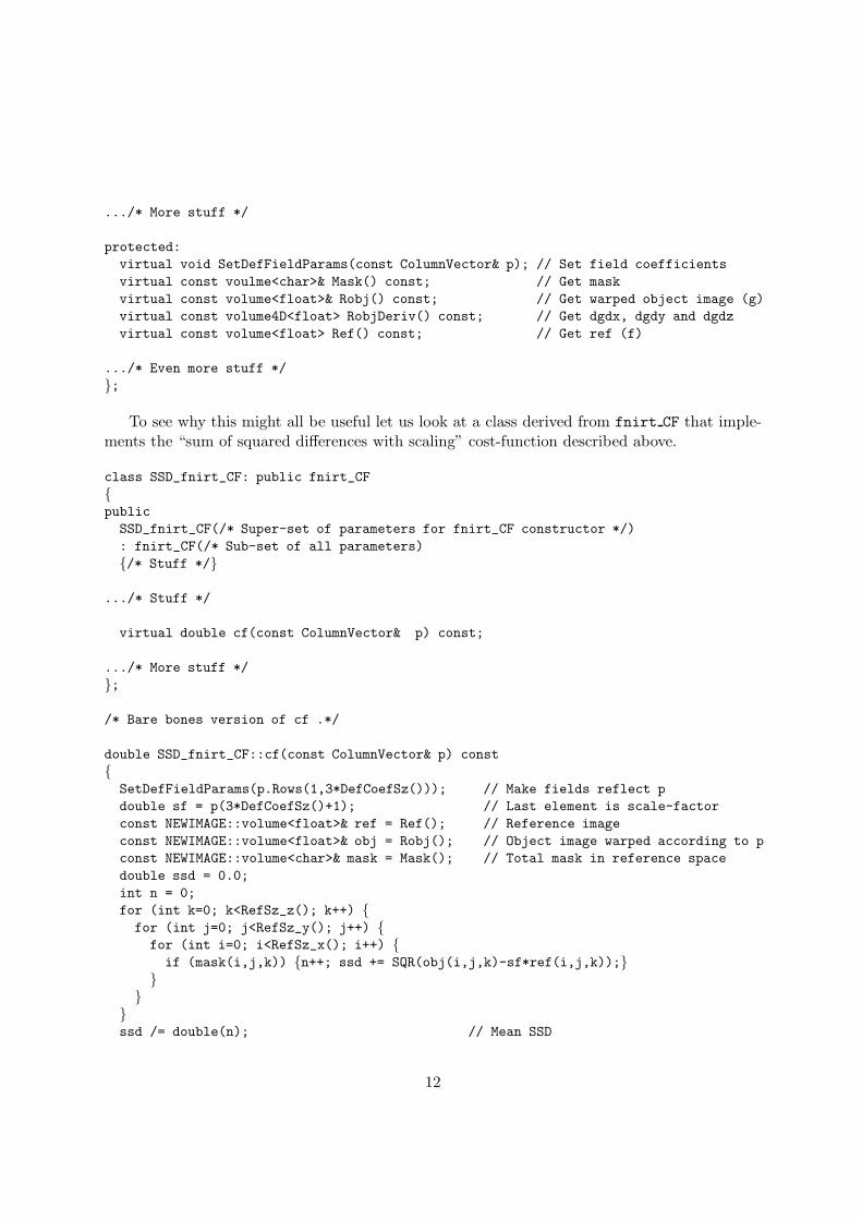
To see why this might all be useful let us look at a class derived from fnirt CF that imple-ments the “sum of squared differences with scaling” cost-function described above.

class SSD_fnirt_CF: public fnirt_CF

{public

SSD_fnirt_CF(/* Super-set of parameters for fnirt_CF constructor */)

: fnirt_CF(/* Sub-set of all parameters)

{/* Stuff */}

.../* Stuff */

virtual double cf(const ColumnVector& p) const;

.../* More stuff */

};

/* Bare bones version of cf .*/

double SSD_fnirt_CF::cf(const ColumnVector& p) const

{SetDefFieldParams(p.Rows(1,3*DefCoefSz())); // Make fields reflect p

double sf = p(3*DefCoefSz()+1); // Last element is scale-factor

const NEWIMAGE::volume<float>& ref = Ref(); // Reference image

const NEWIMAGE::volume<float>& obj = Robj(); // Object image warped according to p

const NEWIMAGE::volume<char>& mask = Mask(); // Total mask in reference space

double ssd = 0.0;

int n = 0;

for (int k=0; k<RefSz_z(); k++) {for (int j=0; j<RefSz_y(); j++) {

for (int i=0; i<RefSz_x(); i++) {if (mask(i,j,k)) {n++; ssd += SQR(obj(i,j,k)-sf*ref(i,j,k));}

}}

}ssd /= double(n); // Mean SSD

12

return(ssd);

}

and SSD fnirt CF may be used in an applictaion like e.g. fnirt

volume<float> ref, obj; // Reference and Object image

volume<char> objm; // Used to mask away that nasty tumor in obj

Matrix M; // Affine matrix from fnirt

.../* Read images, mask and affine matrix. */

vector<int> ksp(3,8); // 8 voxels knot-spacing

vector<int> isz(3); // Size of field/ref

isz[0] = ref.xsize(); isz[1] = ref.ysize(); isz[2] = ref.zsize();

vector<shared_ptr<basisfield> > dfield(3); // field

for (int i=0; i<3; i++) {dfield[i] = shared_ptr<splinefield>(new splinefield(isz,ksp));

}

SSD_fnirt_CF mycf(ref,obj,M,dfield);

mycf.SetObjMask(objm);

NonlinPar mypar(mycf.NPar(),NL_LM); // Levenberg-Marquardt often a good choice

if ((NonlinOut status = nonlin(mypar,mycf)) == NL_MAXITER) {cout % << "Rats!" << endl;

}

So, making ones cost-function a subclass of fnirt CF makes it relatively easy to implementthe cost-function. The functionality inherited from NonlinCF makes it easy to perform theactual minimisation and the functionality from fnirt CF facilitates implementing the actualcost-function (and its derivative and Hessian). So in the example above we used a mask inobject space because we didn’t want the warping to be confused by some ghastly growth thathappens to be in poor obj. Because the mask is in the space of the image we attempt to warpit means that it will have to be warped along with obj in each iteration. This is facilitated byfnirt CF offering a public interface .SetObjMask(mask) that allows us to specify the mask andthe protected function .Mask() that returns a mask that is the intersection of all the masks (inobject and/or reference space) that has been set by the user transformed into reference space.

This is just one example of how the functionality in fnirt CF may facilitate the implemen-tation of new cost-functions.

3.5 Regularisation of the field

The chosen model for non-linear registration offers considerable freedom in terms of different con-stellations of warps. It is frequently the case that a large set of different warps (as parametrisedby different instances of w) yields similar values for the cost-function, and in these cases we need

13

some way to decide between them. Furthermore, representing the field as a linear combinationof basis-fuctions ensures that it is smooth and continous but does not not guarantee that it is“one-to-one” and “onto”.

The term “one-to-one” means that no two points in the original space x can map onto thesame point in the warped space x′, a condition which is indicated by the Jacobian determinantof the [x y z] → [x′ y′ z′] transformation becoming zero or negative at one or more grid points.The significance of “onto” is that each point in the transformed space x′ should have a mappingonto some point in the original space x, i.e. there must not be any points in the transformedspace that “cannot be reached”. The “onto” requirement is not really meaningful (i.e. we cannever hope to enforce it) for a discretely sampled function, but the “one-to-one” condition iswidely thought to be important if we are to consider a transform/field as reasonable.

As alluded to above the “one-to-one” requirement is not guaranteed, or even helped, byrepresenting the field by some basis-set. All that guarantees is that when the Jacobian goesnegative it does so gradually (over space). A common solution to these problems is to use someform of “regularisation” on the field. This is simply some differentiable function of the field, orthe parameters of the field, whose value indicates how “likely” we consider that field to be. Itis quite common to use some mechanical analogy such that in the choice between two fields wewill consider e.g. that with a smaller membrane energy to be the more likely. The mechanicalanalogy results in the same set of equations as one obtains from considering the sum-of-squareddifferences cost-function as a likelihood (assuming normal distributed errors) and postulating amultinormal prior on the coefficients of the field. There are forms for the variance-covariancematrix of the prior that corresponds to e.g. membrane energy and bending energy.

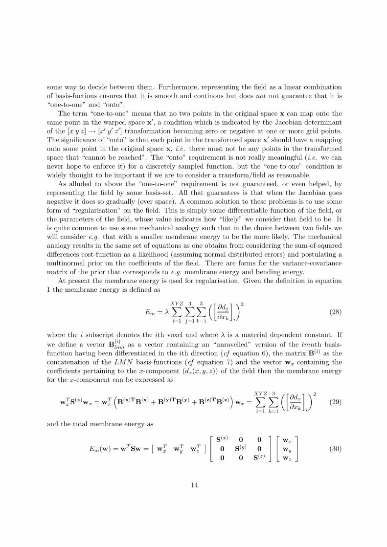
At present the membrane energy is used for regularisation. Given the definition in equation1 the membrane energy is defined as

Em = λXY Z∑

i=1

3∑

j=1

3∑

k=1

([∂dj

∂xk

]

i

)2

(28)

where the i subscript denotes the ith voxel and where λ is a material dependent constant. If

we define a vector B(i)lnm as a vector containing an “unravelled” version of the lmnth basis-

function having been differentiated in the ith direction (cf equation 6), the matrix B(i) as theconcatenation of the LMN basis-functions (cf equation 7) and the vector wx containing thecoefficients pertaining to the x-component (dx(x, y, z)) of the field then the membrane energyfor the x-component can be expressed as

wTx S(x)wx = wT

x

(

B(x)TB(x) + B(y)TB(y) + B(z)TB(z))

wx =

XY Z∑

i=1

3∑

k=1

([∂dx

∂xk

]

i

)2

(29)

and the total membrane energy as

Em(w) = wTSw =[

wTx wT

y wTz

]

S(x) 0 0

0 S(y) 0

0 0 S(z)

wx

wy

wz

(30)

14

Consequently the gradient and the Hessian of Em(w) are

∇Em = Sw (31)

andHEm = S (32)

Hence the cost-function including regularisation, its derivatives and Hessian are

O(θ) =1

XY Z(g(w) − αf)T (g(w) − αf) + λwTSw (33)

,

∇O(θ) =2

XY Z

[JT (w)(g(w) − αf)−fT (g(w) − αf)

]

+ λ

[Sw

0

]

(34)

and

H(θ) =2

XY Z

[JT (w)J(w) −JT (w)f−fTJ(w) fT fT

]

+ λ

[S 0

0T 0

]

(35)

where λ can be seen as an arbitrary weighting of the regularisation versus the sum-of-squareddifferences, or between the likelihood and the prior if one prefers that perspective.

3.5.1 Implementation in the basisfield class

The contribution of the membrane energy is a function only of the field, or rather the parametersdefining the field, and can hence be calculated and returned by the basisfield class. Let us forexample say that we have declared and defined a splinefield like

NEWMAT::ColumnVector w = ...; // Whichever way we get them

BASISFIELD::splinefield xfield(size,knot_spacing);

xfield.SetCoef(w);

we can then obtain the mebrane energy and its gradient and hessian at this point in parameterspace as

double membrane_energy = xfield.MemEnergy();

NEWMAT::ColumnVector gradient = xfield.MemEnergyGrad();

boost::shared_ptr<MISCMATHS::BFMatrix> hessian = MemEnergyHess();

3.5.2 What is going on with that BFMatrix class?

The Hessian H will rapidly become very large and costly to store and calculate (more aboutthe latter below). A reasonable “bread-and-butter” resolution may be, in the case of using aspline-basis, a 4× 4× 4 voxel knot-spacing over the 91× 109 × 91 matrix of the MNI template.This would result in 25 × 30 × 25 splines requiring 18750 parameters for each of the x-, y- andz-displacement fields. This means that H is a 56251 × 56251 matrix, requiring on the order of25GB to store and represent it, something which is beyond most computers today. This is thereason why for example the DCT-based registration in SPM is limited to a resolution of roughly20mm (or 10 voxels) isotropically. The spline basis set has a great advantage here in that theHessian is sparse, meaning that a large proportion of the entries are zero. And that proportion

15

increases with increased resolution of the warps. No row or column of the Hessian contains morethan 343 (7 × 7 × 7) non-zero elements, and many contain fewer. It is therefore crucial thatwe have an efficient storage format for the Hessian (or for sparse matrices in general) if we areto reap the full benefits of the spline basis-set. At the same time we do not wish to representall Hessian matrices as sparse matrices (e.g. the full Hessian matrices from the DCT basis set)since that will typically increase storage needs by more than 50% and incurr an execution timepenalty when the matrix is indeed full.

This is the reason why our basisfield classes, and also the classes derived from NonlinCF,return an object of type BFMatrix. This is a virtual wrapper-class with two derived classesFullBFMatrix and SparseBFMatrix which has an API that is sufficient for the needs of thedifferent sub-classes of NonlinCF. This is a way to obtain the required polymorphism given therestriction that the matrix-class we commonly use, Newmat, do not have a sparse representationnor has it been designed such that it would be easy to sub-class a sparse-matrix class from it.

Why do we then bother to include the DCT basis-set in the first place? When performinglow-resolution ( 20mm warp resolution or poorer) non-linear warping the full Hessian for theDCT set is feasible to represent and very efficient to calculate. This has to do with the propertiesof the basis and slightly simplified it can be though of as an FFT for Hessian calulation. Incontrast the Hessian for the spline set is not very sparse at that resolution, and each element isquite costly to calculate because of the large overlap (in units of voxels) of neighbouring splines.The DCT-set will therefore yield similar results as the spline-set for an order of magnitudeshorter execution time.

The advantage of the spline-set becomes obvious when going to medium-resolution regis-tration ( 10mm warp resolution), when it is no longer possible to represent the full Hessianfor the DCT-set. Even if it was possible to represent it the Hessian contains 64 times moreelements, each element taking as long to compute as for the low-resolution case. For the splineset the number of elements grow much more slowly with increasing reolution since sparsity alsoincreases with resolution. In addition the cost of calculating each element decreases since theoverlap between neighbouring splines decreases. In fact there is but limited difference in the timeit takes to calculate the 5616× 5616 Hessian for a knot-spacing of 20mm and the 31752× 31752Hessian for a 10mm knot-spacing.

3.6 Approximations for speed

When using Gauss-Newton style optimisation (Levenberg or Levenberg-Marquardt) the costliestoperations are the calculation and inversion of H. The example in the preceeding section showsthat a 56251 × 56251 Hessian is in no way unreasonable, and will take a little while both tocompute and invert. For this reason the .JtJ() routines of the derived classes of basisfield

are the real bottle necks, and efforts at optimisation should focus on these.If we look at e.g. equation 19 we see that H is a function of w and will thus need to

be recalculated at each iteration. If we further look at equations 7 and 8 we see that thatdependence comes from caculating ∂g/∂x (and y and z) at the point w in the parameter space.What then do we think ∂g/∂x would look like when we are reasonable close to convergence? Ithink it would look very similar to ∂f/∂x, and that doesn’t depend on w. So one trick, thathas been played successfully in e.g. SPM, is to calculate H once and for all using ∂f/∂x. The

16

approximation is of course worse for the first few iterations when g and f are still quite dissimilar.However, at that stage the second order Taylor expansion that underlies Gauss-Newton styleminimisation is likely to be a poor approximation anyway. It should also be noted that gettingH “wrong” in a Levenberg/Levenberg-Marquardt minimisation should not affect the end result,just the way and time it takes to get there. A poor approximation to H would mean that itwould take more iterations to converge, but on the other hand that should be weighed againstthe time and computational effort of each iteration which will be much smaller if we can reuseH. Even better, of course, would be if we could in the first iteration calculate the Choleskydecomposition of H which would greatly facilitate solving for θ in subsequent iterations.

These are all things that we need to look into empirically. It is neither clear that we will endup using Gauss-Newton style optimisation as our default. In particular the Scaled ConjugateGradient method seems to do well on the model examples I have looked at, and that doesaway with calulating H altogether (though it calculates the gradient twice at each iteration).However, see my reservations below regarding different scales of different sets of parameters.

3.7 Scaling of the gradient vector

Many algorithms for non-linear optimisation suffers quite badly when different parts of thegradient vector (∇O) have vastly different scales. Consider ∇O given by equation 25. It is a3LMN + 1 × 1 vector where the upper 3LMN elements are of the form jTi (g(w) − αf) whereji is a vector which is non-zero only over small portion corresponding to the support of splinethat it pertains to. This is in contrast to the final element −fT (g(w) − αf) where more or lessall elements of f are non-zero. Intuitively it is also obvious that a unity change of α (say from 1to 2) will change O massively, whereas a unity change of one of the spline coefficients will movethe samling point for a few hundred voxels to varying degrees and will have much smaller effecton O. So we have a vector where 3LMN elements are of one scale, and then one element thatis hundreds, or even thousands, of times larger.

Let us then consider what would happen when a method that bases its step (in parameterspace) on the gradient, i.e. attempts to take a step in the −∇O(θ) direction. That directionwill be completely dominated by the α direction, i.e. we attempt to take a long step in the αdirection and a short step in all other directions. The problem though is that most likely we onlyneed to take a very short step in the α direction. If we have done an intial global normalisation(as one does) a realistic range might be 0.97 < α < 1.03. So that means that for the stepθ

(k+1) = θ(k) − λ∇O(θ) we will find a very small λ, and therefore it is likely that we will only

have taken a tiny step of that we would need to take for the other direction. We should note herethat although the search directions for e.g. Variable-Metric and Conjugate-Gradient methodsare not the gradient, they both start ot with that as their initial direction. And because of theway they construct new directions based on previous directions and the present gradient eachnew directions will have a large proportion of the present gradient in them.

In practice what will tend to happen is that for the first few (can be a small few, butsometimes a large few) attempted steps the gradient will be dominated by −fT (g(w) − αf)so the step lengths become very small and we practicaly do not move at all in any of the w

directions. Then comes a step where we are literally at the bottom of the pass in the α directionand ∂O/∂α becomes (very close to) zero. The algorithm will then be able to take a sizeable

17

step along the w directions and the cost-function will decrease. After that step α is typicallynon-zero again and there will be another few steps of neglible length until ∂O/∂α is again zeroand the algorithm will again be able to take a “proper” step. So, the problem produces verytypical symptoms of slow and jerky convergence. For the particular case of a single scale-factorwhose scale is vastly different from the warp parameters (w) it is relatively easy to “fudge” itby redefining O as a summation over (gxyz(w) − (1 + cα)fxyz)

2 where c is some suitably smallconstant (10−3 seems to work reasonably well). However the problem is more “general” thanthat and for example for my top-down-bottm-up method the parameter vector θ = [wTpT ]T

where w is a set of spline-coefficients used to model the (magnetic) field and p are a set ofrigid body movement parameters describing any change in subject position between the twoacquisitions. The effects on the cost-function is of course much larger for any of the movementparameters than for the warp parameters, and we have again a problem of different scales ofparameters. We will see similar problems also if/when we want to include a model for RFinhomogeneity. I suspect/hope it shall be possible to find reasonable fudge factors also for thoseparameters, but it won’t be pretty. It is hardly realistic that we shall be able to find a generalsolution to it since this is a long standing issue in “non-Newton” non-linear optimisation.

In contrast, for the Newton/Gauss-Newton style algorithms this is a non-issue. If we takeagain the example of the gradient described by equation 25, remember that the step for aNewton style algorithm is of the general form θ

(k+1) = H(θ)−1∇O(θ) and look at the elementin the bottom-right corner of H we see that that, just as the large element of ∇O, that too ismuch larger than the other elements of H. A, very crude, approximation to the α componentof the Newton-step is −fT (g(w) − αf)/fT f , and in practice this typically turns out to be oneof the smallest components of the step. The information in the Hessian will for all practicalpurposes “calibrate” any akward scalings in the gradients without any need for finding onesown fudgy factors. This means that convergence tend to be steady and reliable, which makes iteasy to implement convergence criteria. Non-Newton type algorithms, as described above, willfor poorly scaled parameters exhibit long stretches of sometimes tens of iterations during whichchanges in cost-function are very small, and may then all of a sudden make another “jerk” andchange by maybe a factor of two (I have seen it happen). How, then, does one implement a testfor convergence?

Intrestingly the Variable-Metric methods are actually supposed to be able to handle thistype of problem (hence the name), but in my practical tests I have found nothing to indicatethat would actually be the case.

For this reason I tend to favor Gauss-Newton type algorithms over the various flavours ofVariable-Metric/Conjugate-Gradient methods out there that doesn’t require calculation or rep-resentation of the Hessian. Although the price of course is that it complicates the implementationquite considerably and represents a large proportion of the total calculations.

4 EXPERIMENTS

Experiments have been performed registering different structural images against each otherand against templates acquired with similar tissue contrasts. This has been performed bothfor T1-weighted and FA (Fractional anisotropy) images. Tests have been aimed at finding

18

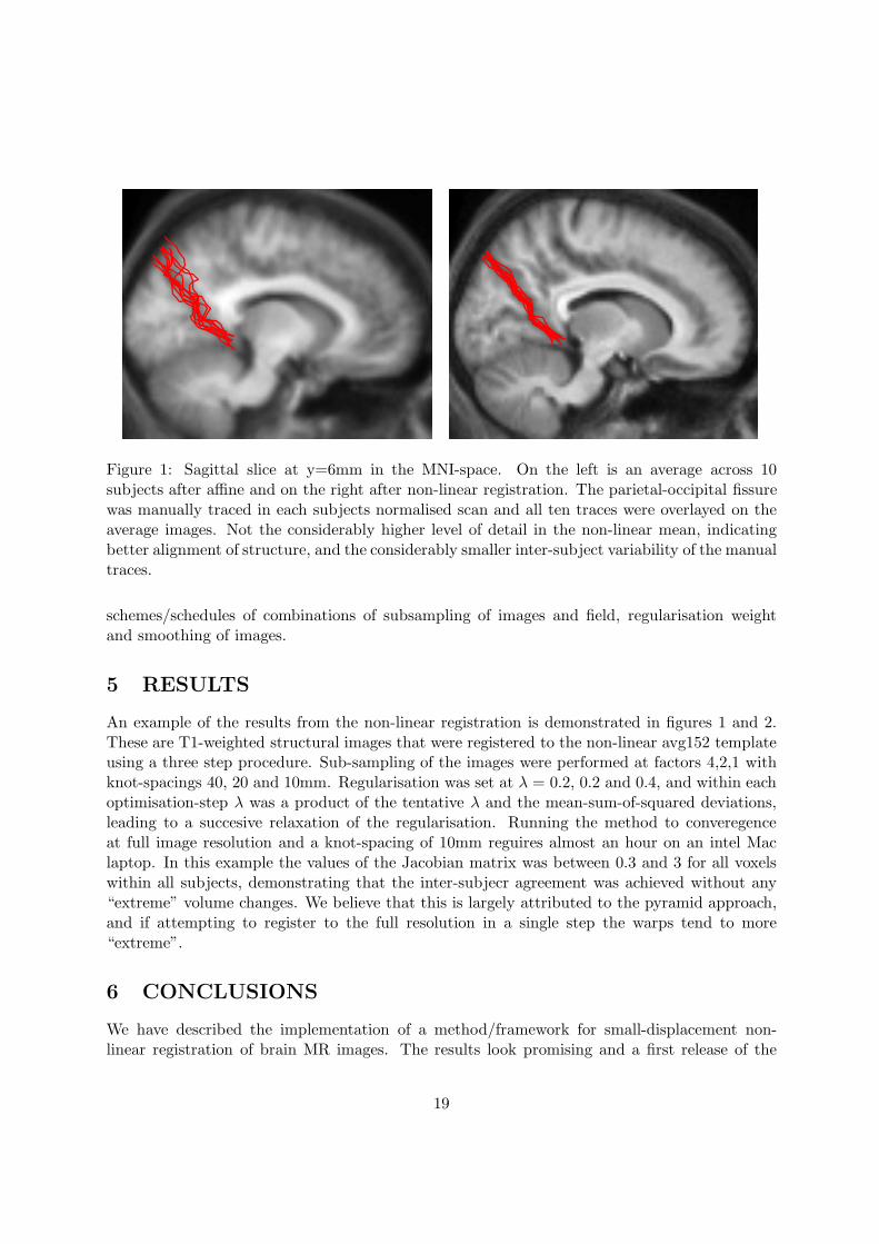
Figure 1: Sagittal slice at y=6mm in the MNI-space. On the left is an average across 10subjects after affine and on the right after non-linear registration. The parietal-occipital fissurewas manually traced in each subjects normalised scan and all ten traces were overlayed on theaverage images. Not the considerably higher level of detail in the non-linear mean, indicatingbetter alignment of structure, and the considerably smaller inter-subject variability of the manualtraces.

schemes/schedules of combinations of subsampling of images and field, regularisation weightand smoothing of images.

5 RESULTS

An example of the results from the non-linear registration is demonstrated in figures 1 and 2.These are T1-weighted structural images that were registered to the non-linear avg152 templateusing a three step procedure. Sub-sampling of the images were performed at factors 4,2,1 withknot-spacings 40, 20 and 10mm. Regularisation was set at λ = 0.2, 0.2 and 0.4, and within eachoptimisation-step λ was a product of the tentative λ and the mean-sum-of-squared deviations,leading to a succesive relaxation of the regularisation. Running the method to converegenceat full image resolution and a knot-spacing of 10mm reguires almost an hour on an intel Maclaptop. In this example the values of the Jacobian matrix was between 0.3 and 3 for all voxelswithin all subjects, demonstrating that the inter-subjecr agreement was achieved without any“extreme” volume changes. We believe that this is largely attributed to the pyramid approach,and if attempting to register to the full resolution in a single step the warps tend to more“extreme”.

6 CONCLUSIONS

We have described the implementation of a method/framework for small-displacement non-linear registration of brain MR images. The results look promising and a first release of the

19

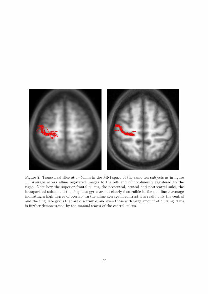
Figure 2: Transversal slice at z=56mm in the MNI-space of the same ten subjects as in figure1. Average across affine registered images to the left and of non-linearly registered to theright. Note how the superior frontal sulcus, the precentral, central and postcentral sulci, theintraparietal sulcus and the cingulate gyrus are all clearly discernible in the non-linear averageindicating a high degree of overlap. In the affine average in contrast it is really only the centraland the cingulate gyrus that are discernible, and even those with large amount of blurring. Thisis further demonstrated by the manual traces of the central sulcus.

20

software is scheduled to July 2007. Future work will aim at validation, finding the best setof parameters/schedules for different types of images and at a better modelling of the signalby including bias-field, and a physics based mapping of intensities between the two image (orbetween the template and the input image).

21