1

Non-Linear Constrained Optimal Control Problem: A PSO-GA-Based Discrete Augmented Lagrangian Approach

1Faculty of Business Administration, University of New Brunswick, Fredericton, E3B 5A3, Canada 2Department of Systems Engineering, King Fahd University of Petroleum and Minerals, Dhahran 31261, Saudi Arabia

Correspondence should be addressed to Haris M. Khalid, mhariskh@kfupm.edu.sa

Abstract— This work deals with the optimal control problem which has been proposed to solve using the discrete augmented

lagrangian based non-linear programming approach. It is shown that this technique guarantee a satisfactory performance in the face of both

optimality by minimizing the energy and maximizing the output. Later on, the optimization has been more effective by using PSO-GA-

Based to achieve the optimal value of Lagrange Multipliers and required dynamic parameters and optimally controlling the dynamics. The

designed scheme has been successfully tested through extensive simulation. The successful use of the proposed scheme encourages their

extension to other physical systems. The proposed scheme is evaluated extensively on a two-tank process used in industry exemplified by a

benchmarked laboratory scale coupled-tank system.

Keywords — optimal control, augmented lagrangian, non-linear programming, particle swarm optimization, genetic algorithm,

control of two-tank system.

I. INTRODUCTION

Many processes in chemical and biotechnological industries are described by multiple sets of differential and algebraic

equations. As such they are difficult to control and optimize in transient regimes if switching between the sets is to be taken

into account. The switches can involve different regimes of operation (occurrence of flooding in distillation columns,

explosive areas in mixtures of gasses, etc) or external actions (addition of second reactor when production increases, etc). In

theoretical and numerical research, optimal control problems have been either treated as cone constrained optimization

problems in functional spaces, or studied using some specialized tools. In the first approach, problems of optimal control are

placed in a broader framework of optimization problems, and general techniques can be used to solve them, whereas the

second approach allows us to take maximal advantage of the specific structure of the problems. Such a situation takes place

also in applications of the methods involving Lagrangian for solving numerically optimal control problems.

The paper is organized as follows: in Section II the related work is presented and Optimal Control problem statement is

considered in Section III. Section IV gives the system model and description, Section V discusses the implementation and

simulation results for all the techniques implemented. Finally some conclusions are given Section VI.

II. RELATED WORKS

There are several approaches to solution of such as dynamic optimization problem. If the process to be optimized can be

described accurately enough by piece-wise linear and logic formulation, powerful algorithms in the area of explicit model

predictive control exists [1]. If fully nonlinear processes are concerned, original dynamic optimization problem has to be

approximated by some simplified formulation. The usual approaches are complete discretisation of state and control variables

– orthogonal collocation. Such formulation can be found in [2]. Other possibility is to leave the states intact and approximate

only the control variables as piece-wise constant, or with some higher order approximations. This approach is known as

M.A. Rahim1, Haris M. Khalid2, S.Z. Rizvi2 and Amar Khoukhi2

2

control vector parameterization. Here different formulations can be found, depending on how gradients of the resulting

nonlinear programming problem (NLP) are calculated. In [3], system of sensitivity equations is formed and the gradients are

calculated from its solution. The advantage of this method is easy formulation of the problem and forward integration of both

states and sensitivity equations. The drawback of this method lies in a large system of differential equations as each

optimized parameter generates a set of differential equations with the same dimension as the number of states of the

optimized process. Another possibility, which is pursued in this work, is to calculate the gradients of NLP via optimal control

theory using the so-called co-state, or adjoint equations [4]. The advantage is that the number of differential equations is not

proportional to number of optimized parameters, but to number of constraints. On the other side, adjoint equations have to be

solved in opposite direction of time which makes the implementation more difficult. When dealing with processes comprised

of a large number of state equations and only a small number of state-dependent constraints, this approach has favorable

properties compared to calculation of sensitivities.

The classical Lagrange-Newton method [5], one of the most efficient numerical methods of solving optimization problems,

was developed for problems with equality-type constraints. In this method, the Newton procedure is applied to the first-order

optimality system, which has the form of a system of equations. In the case of inequality-type constraints, the first-order

optimality system cannot be expressed as an equation. However, it can be expressed as an inclusion, or the so-called

generalized equation [6]. It was shown by S.M. Robinson [6] that a Newtontype procedure applied to this general equation is

locally quadratically convergent to the solution, provided that a property called strong regularity is satisfied. This approach

has been successfully applied to a class of nonlinear cone-constrained optimization problems in infinite dimensional spaces

[7][8][9] and optimal control problems subject to control and/or state constraints[10]. Hybridizing the classical optimization

technique with evolutionary algorithms can be a good proposed option.

Genetic Algorithms (GAs) are a special type of evolutionary algorithms, algorithms that simulate biological processes to

solve search and optimization problems. Given a specific problem, potential solutions are typically encoded as bit strings,

constituting a population. The bit strings are allowed to reproduce on the basis of their fitness, thus forming a new population.

Iterating this process, the population evolves according to a ‘natural selection and survival of the fittest’ process similar to the

one described by Charles Darwin in the Origin of Species. If the GA is implemented successfully, the final population should

consist of maximally-fit it individuals, approximating the sought optimal solution. GAs have been implemented for a wide

variety of problems, both real-world (e.g. Fault diagnosis, fault tolerant) and abstract (e.g. solving NP-complete problems [11]).

The bulk of the GA literature is concerned with practical applications. For a very complete bibliography, see [12], which

contains a comprehensive survey. PSO has attracted much attention among researchers and has been used to solve complex

optimization problems with wide applications in different fields [13].

Khoukhi et al. has also done considerable work in optimal dynamic modeling and optimal time-energy off-line

programming [14-16].

The main aim of this work is to show a detailed derivation of the dynamic Augmented Lagrangian Based optimization based

on the optimal control theory. The results obtained will then be presented on an example of benchmarked laboratory scaled two

tank level control that exhibits non-linear dynamics. It is the most used prototype applied in the wastewater treatment plant, the

petro-chemical plant, and the oil/gas systems. The main contribution of the paper is the implementation of PSO-GA-Based

optimal control of augmented lagrangian functions.

3

III. PROBLEM STATEMENT

Complex optimal control problems require a serious attention for surviving smartly in the process industries. Many units

in process industries are described by multiple sets of differential and algebraic equations. Many complex control tasks, for

example those associated with controlling an autonomous vehicle to carry out a sequence of maneuvers or with controlling a

collection of interacting process units in a process plant, involve two levels of decision making. At the maximum level, it is

necessary to achieve a certain maximum output whereas at the same time, at the minimum, it is required to minimize the

certain possibility of fault. Hybrid control addresses the problem of integrating the minimization and maximization for

decision making in this context. The early optimal control of mission critical systems becomes highly crucial for preventing

failure of equipment, loss of productivity and profits, management of assets, reduction of shutdowns.

Figure 1. Implementation plan for the evaluation of the proposed scheme

The proposed scheme has been evaluated on the above- cited process control system. The scheme is carried out by jointly

interpreting model outputs. The implementation plan for the proposed scheme is shown in the Fig 1. It should be noted that

PSO-GA-Based NLP Constrained optimization is applied for the optimal control of the system.

IV. SYSTEM MODEL AND DESCRIPTION

A. System Description

The Benchmarked laboratory-scale process control system has been used to collect data. The data has been collected at a

sampling time of 50 milli-second. The different data sets have been generated for PI Control-based water level control.

Different fault scenarios have also been considered for the generation of the data sets.

B. Experimental Setup

Process Data has been generated through an experimental setup as shown in Figure 2. A two tank system has been used in

order to collect the data with the introduction of actuator, and sensor faults through the system as can be seen in the labview

circuit window. An amplified voltage of 18 volts has been used to handle the controller effectively for the changes/fluctuation

produced in the system. So, the fault diagnosis was done over here in a closed loop identification where in the same time, the

controller is suppressing the faults.

4

C. Process Data Collection and Description

The process data has been collected at 50 milli-seconds sampling time. The main objective of the benchmarked dual-tank

system is to reach a reference height of 200 ml of the second tank. During this process, several faults have been introduced

such as the leakage faults, sensor faults and actuator faults. Leakage faults have been introduced through the pipe clogs of the

system, knobs between the first and the second tank etc. Sensor faults have been introduced by introducing a gain in the circuit

as if there is a fault in the level sensor of the tank. Actuator faults have been introduced by introducing a gain in the setup for

the actuator that comprises of the motor and pump. A PI controller has been employed in order to reach the desired reference

height. Due to the inclusion of faults, the controller was finding it difficult to reach the desired level. For this reason, the power

of the motor has been increased from 5 volts to 18 volts in order to provide it the maximum throttle to reach the desired level.

In doing so, the actuator performed well in achieving its desired level but it also suppressed the faults of the system. So, it

made the task of detecting the faults. After the collection of data, techniques such as settling time, steady state value, and

coherence spectra can help us to give an insight of the fault.

Figure 2 A – The two tank system interfaced with the Labview through a DAQ and the amplifier for the magnified voltage , B – The labview setup of the apparatus including the ciruit window and the block diagram of the experiment.

D. Model of the Coupled Tank System

The physical system under evaluation is formed of two tanks connected by a pipe. The leakage is simulated in the tank by

opening the drain valve. A DC motor-driven pump supplies the fluid to the first tank and a PI controller is used to control the

fluid level in the second tank by maintaining the level at a specified level, as shown in Fig 3.

A step input is applied to the dc motor- pump system to fill the first tank. The opening of the drainage valve introduces a

leakage in the tank. Various types of leakage faults are introduced and the liquid height in the second tank, 2H , and the inflow

rate, iQ , are both measured. The National Instruments LABVIEW package is employed to collect these data.

A benchmark model of a cascade connection of a dc motor and a pump relating the input to the motor, u, and the flow, iQ ,

is a first-order system:

( )i m i mQ a Q b uφ= − +ɺ (1)

5

where ma and mb are the parameters of the motor-pump system and ( )uφ is a dead-band and saturation type of nonlinearity.

It is assumed that the leakage Qℓ occurs in tank 1 and is given by:

12dQ C gH=ℓ ℓ

(2)

With the inclusion of the leakage, the liquid level system is modeled by:

( ) ( )11 12 1 2 1i

dHA Q C H H C H

dtϕ ϕ= − − −

ℓ (3)

( ) ( )22 12 1 2 0 2

dHA C H H C H

dtϕ ϕ= − − (4)

where (.) (.) 2 (.)sign gϕ = , ( )1Q C Hϕ=ℓ ℓ

is the leakage flow rate, ( )0 0 2Q C Hϕ= is the output flow rate, 1H is the height

of the liquid in tank 1, 2H is the height of the liquid in tank 2, 1A and 2A are the cross-sectional areas of the 2 tanks,

g=980 2/ seccm is the gravitational constant, 12C and oC are the discharge coefficient of the inter-tank and output valves,

respectively.

The model of the two-tank fluid control system, shown above in Fig. 3, is of a second order and is nonlinear with a smooth

square-root type of nonlinearity. For design purposes, a linearized model of the fluid system is required and is given below in

(5) and (6):

( )11 1 1 1 2i

dhb q a h a h

dtα= − + + (5)

( )22 1 2 2

dha h a h

dtβ= − − (6)

where 1h and 2h are the increments in the nominal (leakage-free) heights 01H and 0

2H :

01 1 0 0 0

1 1 2 2

1, ,

2 2 ( ) 2 2

dbC Cb a

A g H H gHβ= = =

−, 2 1 0 0

2 12 2 2 2

do dC Ca a

gH gHα= + = ℓ

and the parameter α indicates the amount of leakage.

Fig. 3 Process control system: A Lab-scale two-tank system

A PI controller, with gains pk and Ik , is used to maintain the level of the Tank 2 at the desired reference input r as:

6

3 2

3p I

x e r h

u k e k x

= = −

= +

ɺ

(7)

The linearized model of the entire system formed by the motor, pump, and the tanks is given by:

x Ax Br y Cx= + =ɺ

(8)

where

1 1 11

2 22

3

0

0 0, ,

1 0 0 0

0

0 0 1 , [1 0 0 0]

i m p m I m

T

m p

a a bh

a ahx A

x

q b k b k a

B b k C

α

β

− − − −

= = − − −

= =

(9)

where iq ,qℓ

, 0q , 1h and 2h are the increments in iQ ,Qℓ, oQ , 0

1H and 02H , respectively, the parameters 1a and 2a are

associated with linearization whereas the parameters α and β are respectively associated with the leakage and the output

flow rate, i.e. 1q hα=ℓ

, 2oq hβ= .

Proposition: During the implementation process, sign(.) can be approximated with arc tangent. A relationship for approximation can be

as follows:

( ) arctan( ), 11 *

xsign x where x

x x= <

−

Likewise, after approximation, the profiles can be as follows: (See Fig. 4) where (a) representing the sign(.) profile and (b)

representing the arctangent profile for a certain set of numbers.

1 2 3 4 5 6 7 8 9-2

-1.5

-1

-0.5

0

0.5

1

1.5

2

x-axis

y-ax

is

arc sine profile

0 2 4 6 8 10 12 14 16 18

-1.5

-1

-0.5

0

0.5

1

1.5

x-axis

y-ax

is

arctangent profile

(a) (b)

Fig. 4 (a) sign(.) profile and (b) Arctangent profile for a certain set of numbers

V. IMPLEMENTATION AND SIMULATION RESULTS

The tasks of our optimal control scheme, are executed with an increasing precision accompanied with a more detailed

optimality picture. Firstly, the data collected from the plant has been initialized and the parameters are being optimized which

comprises of the pre-processing and normalization of the data and applying the Kalman filter to obtain the feasible solution.

Then, the estimation of states based on updated Lagrangian multipliers, and the penalty parameter estimate updates are being

done followed by the iterative aggregated updates. To have a cross-optimal solution, the functions have been optimized using

PSO-GA-Based approach. The flowchart of the implementation can be seen in the Figure 6.

7

A. Kalman Filter-Based Feasible solution for Optimal Control

Using the leakage-free model together with the covariance of the measurement noise, R, and the plant noise covariance, Q,

the Kalman filter model is finally derived. As it is difficult to obtain an estimate of the plant covariance, Q, a number of

experiments were performed under different plant scenarios to tune the Kalman gain, 0K obtained by:

( )0 0 0 0ˆ ˆ ˆ( 1) ( ) ( ) ( ) ( )x k A x k B u k d K y k C x k+ = + − + − and 0 ˆ( ) ( ) ( )e k y k C x k= − . The initial feasible solution for the Kalman

filter filter can be shown in Figure 5 where height profile is shown in the upper window and the kalman filter residual

analysis is shown in the lower window.

0 500 1000 1500 2000 25000

50

100

150

200

time

heig

ht

The height profile and the residual of Kalman filter

0 500 1000 1500 2000 2500-10

-5

0

5

time

resi

dual

residual

Figure 5. Kalman filter residual analysis considered as feasible solution

B. Cost Function of the System

2 2 21 2

1 1 1( ) ( )

2 2 2pL H t H t u= − − + (10)

Constraints:

1 1 12 1 2 1 2 1 11

1( 1) ( ) [ ( arctan( ) 2 ( ) arctan( ) 2 )]*i l sH t H t Q C H H g H H C H gH T

A+ = + − − − − (11)

2 2 12 1 2 1 2 0 2 22

1( 1) ( ) [ ( arctan( ) 2 ( ) arctan( ) 2 )]*sH t H t C H H g H H C H gH T

A+ = + − − − (12)

( 1) ( ) [ arctan( ) 2 ( ) ( )]*i i m m i sQ t Q t b u gu t a Q t T+ = + − (13)

12 0L dlQ C gH− = (14)

2 0e r H− + = (15)

3 0p Iu k e k x− − = (16)

8

Optimal Control using Augmented Lagrangian Algorithm Approach

Data Pre-treatment and Reading: Gather data from the setup → Samples of data required to extract the feasible solution from kalman filter → Initial and Final States, state components and sampling periods N, and iterations T* are considered to be the root definition of the embedded data → Model Extraction: state space model of the system (A0_fault(fp=N/A),……, D0_fault(fp=N/A)) where fp: fault potency considered to be healthy.

Continuous time system→ Discrete time system→ Cost Function→ Energy Minimization with Output Flow and level of Height Maximization

2 2 2 20 2 1 2

1 1 1 1( 2 ( )) ( ) ( )

2 2 2 2dE C gH t H t H t u= − − −

Feasibility Test: / 4v dE w∇ <

Convergence Test *

tw w<

Convergence achieved with precision: * * *1,w andη η

Convergence optimal trajectory: * * *( ) , ( ) , ( )k k l k k l k k lx x h h v v= = =

Estimation of states Based on Updated Lagrange Multipliers:

1 1

0,1,.....,

( ), (1 ) ( )t t t tk k st k k gt gt g

for k N

σ ρ µσ σ µ Ψ σ ρ ρ µ µ Ψ ρ+ +

== + ∇ = − + ∇

Penalty Parameter Estimate Updates: 1 1

1

0,1,....., ,t t t tk k k k

t t t

for k N

update penalty by decreasing it

ρ ρ σ σµ υ µ

+ +

+

= = ==

Iterative Aggregated Updates: Put 1 1max ( , )k i icα µ+ += , If final convergence test holds (e.g.

k toleranceτ ≤ ) exit, Else 1 *1 ( )k k k kc xλ λ µ −

+ = − Choose 1 (0, )k kµ µ+ ∈ Choose a new starting point xk+1, e.g. xk+1 =

xk*. End

Optimized Updates through PSO-GA: Optimization of global best solution using initial population generation, fitness function evaluation, elite chromosomes, cross-over and mutation.

Kalman Filter Based Inner Optimization: Time-energy Feasible Solution Initial Solution Based Inner optimization for control input u using Kalman Filter where αi denotes the leakeage and Yi denotes the Height of water. Backward computation of the co-states, , 1,......,0k k Nλ = −

:

h

Dv

Compute gradients

Lµ∇

^ ^ ^ ^2 * * 1

1 1/, 0 / 1 0 , / 1 0 , , 0 ,

* * *1 / / 1 , , , 2

, , ( , ) * ,

1( )

leak leak leak leaki i i ie i n N P i i f i i i e i N P f i f i ii

i i i i i f i e i f in

R I C P C K P C R I K C K Y F

P F P K R K F GG

σ α α α α

σ

−− ++ − − +

+ −

= + = = − + =

= − +

N0O

YES

Figure 6. Flowchart for the implementation of the proposed scheme

Bounds:

1) Qi ≥0, Qi ≤ 200

2) Q0 ≥0, Q0 ≤ 200

3) 0≤ H1 ≤ 200

4) 50≤ H2 ≤ 200

YES

9

4) u ≥ 5, u ≤ 18

5) C0 ≥ 0.25, C0 ≤ 1.0

6) C1 ≥0.25, C1 ≤ 1.0

7) am ≥ 0, am ≤ 18

8) am ≥ 0, bm ≤ 18

Where

Q0 represents the output flow rate.

kp represents the proportional gain of the controller.

kI represents the integral gain of the controller.

H1 represents the Height of the first tank.

H2 represents the Height of the second tank.

Qi represents the Initial flow of water

am represents the motor system

bm represents the pump system

C12 represents the Discharge coefficient of Inter-tank

C0 represents the Discharge coefficient of output valves

C. Augmented Lagrangian Method for Optimal Control

C.I. Lagrangian Algorithmic Framework of Optimal Control

The augmented lagrangian multiplier method combines the lagrange multiplier and the penalty function methods. The augmented Lagrangian function is given as:

2

1 1

( , , ) ( ) ( ) ( )p p

k j j k jj j

A X r f X h X r h Xα α= =

= + +∑ ∑

Where rk is the penalty parameter. It can be noted that the function A reduces to the Lagrangian if rk=0.

10

Figure 7. Flowchart for the augmented largrangian multiplier Algorithm method for optimal control

Given 0 0 00,x andµ λ> and final tolerance tolerance,

For k = 0,1,2,…….

Starting with xk minimize ( , ; )A k kL x λ µ terminating when

( , ; )A k k kL x λ µ τ∇ ≤

Call the result *kx

If final convergence test holds (e.g. k toleranceτ ≤ ) exit

Set k=1

Augmented Lagrange multiplier Algorithm method

Start with initial values X(1), λ(1), r1, c >1,

Minimize A(X, λ(k), rk) from starting point X (k) and find X * (k)

Check for the convergence of X (k) and X * (k)

Set λj(k+1)= λj

(k) + 2rkhj (X * (k)), j=1,2,…..,p

Set rk+1 = crk

If rk+1 > rmax , set rk+1 = rmax

Set k=k+1

Take X*= X*(k) and stop

NOT CONVERGED

Basic Concept

� L(X, λ) is called as the Lagrange function, X is the objective function and λ is the lagrange multiplier. � A(X, λ, rk ) is called as the Augmented Lagrange function, X is the objective function, λ is the lagrange multiplier, and rk is the penalty function.

11

Else

1 *1 ( )k k k kc xλ λ µ −

+ = −

Choose 1 (0, )k kµ µ+ ∈

Choose a new starting point xk+1, e.g. xk+1 = xk*.

End

End

This algorithmic framework allows a gentler decrease in µ.

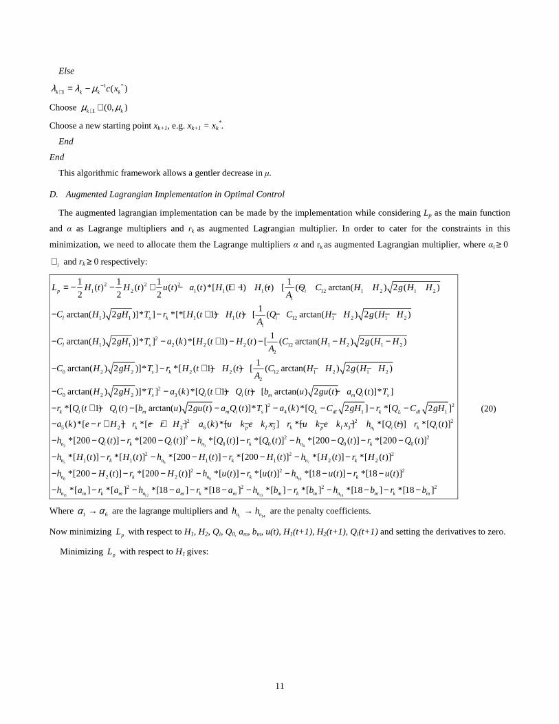
D. Augmented Lagrangian Implementation in Optimal Control

The augmented lagrangian implementation can be made by the implementation while considering Lp as the main function

and α as Lagrange multipliers and rk as augmented Lagrangian multiplier. In order to cater for the constraints in this

minimization, we need to allocate them the Lagrange multipliers α and rk as augmented Lagrangian multiplier, where αi 0≥

i∀ and rk 0≥ respectively:

2 2 21 2 1 1 1 12 1 2 1 2

1

1 1 1 1 12 1 2 1 21

21 1 2 2

1 1 1 1( ) ( ) ( ) ( ) *[ ( 1) ( ) [ ( arctan( ) 2 ( )

2 2 2

1arctan( ) 2 )]* ] *[*[ ( 1) ( ) [ ( arctan( ) 2 ( )

arctan( ) 2 )]* ] ( ) *[ ( 1)

p i

l s k i

l s

L H t H t u t a t H t H t Q C H H g H HA

C H gH T r H t H t Q C H H g H HA

C H gH T a k H t

= − − + − + − − − − −

− − + − − − − −

− − + 2 12 1 2 1 22

0 2 2 2 2 12 1 2 1 22

20 2 2 3

1( ) [ ( arctan( ) 2 ( )

1arctan( ) 2 )]* ] *[ ( 1) ( ) [ ( arctan( ) 2 ( )

arctan( ) 2 )]* ] ( ) *[ ( 1) ( ) [ arctan( ) 2 ( ) ( )]* ]

*[ ( 1)

s k

s i i m m i s

k i

H t C H H g H HA

C H gH T r H t H t C H H g H HA

C H gH T a k Q t Q t b u gu t a Q t T

r Q t Q

− − − −

− − + − − − −

− − + − − −

− + −

1

2 3

2 24 1 1

2 2 25 2 2 6 3 3

2

( ) [ arctan( ) 2 ( ) ( )]* ] ( ) *[ 2 ] *[ 2 ]

( ) *[ ] *[ ] ( ) *[ ] *[ ] *[ ( )] *[ ( )]

*[200 ( )] *[200 ( )] *[

i m m i s L dl k L dl

k p I k p I n i k i

n i k i n

t b u gu t a Q t T a k Q C gH r Q C gH

a k e r H r e r H a k u k e k x r u k e k x h Q t r Q t

h Q t r Q t h Q

− − − − − −

− − + − − + − − − − − − − −

− − − − −4

5 6 7

8 9 10

2 20 0 0 0

2 2 21 1 1 1 2 2

2 22 2

( )] *[ ( )] *[200 ( )] *[200 ( )]

*[ ( )] *[ ( )] *[200 ( )] *[200 ( )] *[ ( )] *[ ( )]

*[200 ( )] *[200 ( )] *[ ( )] *[ ( )] *[18 ( )]

k n k

n k n k n k

n k n k n

t r Q t h Q t r Q t

h H t r H t h H t r H t h H t r H t

h H t r H t h u t r u t h u t r

− − − − −

− − − − − − − −

− − − − − − − − −

11 12 13 14

2

2 2 2 2

*[18 ( )]

*[ ] *[ ] *[18 ] *[18 ] *[ ] *[ ] *[18 ] *[18 ]

k

n m k m n m k m n m k m n m k m

u t

h a r a h a r a h b r b h b r b

−

− − − − − − − − − − − −

(20)

Where 1 6α α→ are the lagrange multipliers and 1 14n nh h→ are the penalty coefficients.

Now minimizing pL with respect to H1, H2, Qi, Q0, am, bm, u(t), H1(t+1), H2(t+1), Qi(t+1) and setting the derivatives to zero.

Minimizing pL with respect to H1 gives:

12

12 1 21 1 1 22

1 1 1 21 2 1 2

11 1 1 122

11 1 1

(( ( ) ( )).1( ) ( 1 [ ( .( 2 ( ( ) ( )) )

2 ( ( ) ( ))1 (( ( ) ( )) 2 ( ( ) ( )

( ( ). 1( .( 2 ( ( )) ) 2 [( ( 1) ( ) [ ( arctan1 ( ( ) 2 ( ( )) 2 ( ( ))

p

Lk i

L C H t H t gH t g H t H t

H A g H t H tH t H t g H t H t

C H t gg H t r H t H t Q C

AH t g H t g H t

α∂ − −

⇒ − − − − − +∂ −+ − −

−− + − + − − −

+ 1 2

2 121 2 1 1 1 22

2 1 2 1 2

1 22 2 12 1 2 1 2 0 2 2

21 2

( )

2 ( ) arctan( ) 2 )]* ] ( ).( 2 ( ( ) ( ))1 (( ( ) ( ( )) 2 ( ( ) ( ))

(( ( ) ( )). 1)) 2 ( ( 1) ( ) [ ( arctan( ) 2 ( ) arctan( ) 2 )

2 ( ( ) ( ))

l s

k

H H

Cg H H C H gH T g H t H t

A H t H t g H t H t

H t H t gr H t H t C H H g H H C H gH

Ag H t H t

α

−

− − + − −+ − −

−− + − − − − −

−

5 64 1 1 1

1

]* )]

( ) 2 [( 2 )] (1) 2 [( )] (1) 2 [(200 )] 02

s

dlk L dl n k n k

T

Cr Q C gH h r H h r H

gHα+ − − − − − − − =

(21)

Minimizing pL with respect to H2 gives:

1 12 1 22 1 22

2 1 1 21 2 1 2

1 1 12 1 2 1 2 1 11

2 12

2 1

(( ( ) ( )).( ) ( .( 2 ( ( ) ( )) )

2 ( ( ) ( ))1 (( ( ) ( )) 2 ( ( ) ( )

12 [( ( 1) ( ) [ ( arctan( ) 2 ( ) arctan( ) 2 )]* ]

( 11 (( (

p

k i l s

L C H t H t gH t g H t H t

H A g H t H tH t H t g H t H t

r H t H t Q C H H g H H C H gH TA

C

A H

α

α

∂ − −⇒ − − − − − −

∂ −+ − −

+ − − − − − − +

− ++

1 21 22

2 1 2 1 2

0 22 2 2 12 12

22 2 2

2 1 2 0 2 2

(( ( ) ( )).).( 2 ( ( ) ( )) ))

) ( ( )) 2 ( ( ) ( )) 2 ( ( ) ( ))

( ( )). 1.( 2 ( ) ) 2 ( ( 1) ( ) [ ( arctan(

1 [( ( ) 2 ( )] 2 ( ( ))

) 2 ( ) arctan( ) 2 )]*

k

s

H t H t gg H t H t

t H t g H t H t g H t H t

C H t ggH t r H t H t C H

AH t gH t g H t

H g H H C H gH T

−− − − −− − −

+ − + − − −+

− −7

8

6 2 2

2

)] (1) 2 [( )] (1) 2 [( )]

(1) 2 [(200 )] 0

k n k

n k

r e r H h r H

h r H

α− − − + − − +

− − =

(22)

Minimizing pL with respect to Qi gives:

1 2

0 3( ) ( )) ( ) (1 ) 2 [( ( 1) ( ) [ arctan( ) 2 ( ) ( )]* )]( )

(1) 2 [( )] (1) 2 [(200 )] 0

pi i m k i i m m i s

i

n k i n k i

LQ t Q t Q t a r Q t Q t b u gu t a Q t T

Q t

h r Q h r Q

α∂

⇒ − + + − + − + − − −∂

− − + − − = (23)

Minimizing pL with respect to Q0 gives:

3 40 0 00

( ( ) ( )) 2 [( )] 2 [(200 )] 0pi n k n k

LQ t Q t h r Q h r Q

Q

∂⇒ − − − + − − =

∂ (24)

Minimizing pL with respect to am gives:

11 12

3( ( )) 2 [( ( 1) ( ) [ arctan( ) 2 ( ) ( )]* )]

2 [( )] 2 [(18 )] 0

pm i k i i m m i s

m

n k m n k m

La Q t r Q t Q t b u gu t a Q t T

a

h r a h r a

α∂

⇒ − − + − − − −∂

− + − − = (25)

Minimizing pL with respect to bm gives:

13

13 14

3 2 2 12 12

2 1 2 0 2 2

1( arctan ( ) 2 ( )) 2 ( ( 1) ( ) [ ( arctan(

) 2 ( ) arctan( ) 2 )]* )] 2 [( )] 2 [(18 )] 0

pm k

m

s n k m n k m

Lb u t gu t r H t H t C H

b A

H g H H C H gH T h r b h r b

α∂

⇒ − − − + − − −∂

− − − − + − − = (26)

Minimizing pL with respect to u(t) gives:

9 10

3 2

( ).( ) ( . 2 ( ) 2 [( ( 1) ( ) [ arctan( ) 2 ( )

( ) 1 ( ( ) 2 ( )) 2 ( )

( )]* )] 2 [( ( ))] 2 [(18 ( ))] 0

p mk i i m

m i s n k n k

L b u t gu t gu t r Q t Q t b u gu t

u t u t gu t gu t

a Q t T h r u t h r u t

α∂

⇒ − − + − + − − −∂ +

− − + − − = (27)

D.I. Solving the derivatives:

Considering all the lagrange multipliers α , minimizing pL with respect to the states gives (See-Equation 28-33):

1 20 3 3( ) ( ) 0m n nQ t a h hα α+ − − + = (28)

11 123( ( )) 0m i n na Q t h hα− − + = (29)

13 143(arctan ( ) 2 ( ) 0m n nb u t gu t h hα+ − + = (30)

9 103 2

( ).( )( 2 ( ) ) 01 ( ( )( 2 ( )) 2 ( )

mn n

b u t gu gu t h h

u t gu t gu tα+ + − + =

+ (31)

7 82 6( ) 0n nH t h hα− − + = (32)

5 61( ) 0n nH t h h− − = (33)

11

22

3

0 (34)( 1)

0 (35)( 1)

0 (36)( 1)

p

p

p

i

L

H t

L

H t

L

Q t

α

α

α

∂⇒ − =

∂ +∂

⇒ − =∂ +

∂⇒ − =

∂ +

Substituting, Equation # (21-36) gives a new formulation (Equation 31, which being dependent onα , we need to

maximize:

1 20 ( ) 0n nQ t h h− + = (37)

11 120m n na h h− + = (38)

13 140m n nb h h− + = (39)

3 40( ) ( ) 0i n nQ t Q t h h− − + = (40)

9 105 0n nu h hα+ − + = (41)

5 61 4

1

( ) ( ) 02

dln n

gCH t h h

gHα− − + = (42)

14

7 102 6( ) 0n nH t h hα− − + = (43)

1 1 1 12 1 2 1 2 1 11

2 2 2 12 1 2 1 2 0 2 22

3

1( 1) ( ) [ ( arctan( ) 2 ( ) arctan( ) 2 )] (44)

1( 1) ( ) [ ( arctan( ) 2 ( ) arctan( ) 2 ) (45)

( 1) ( ) [ arctan( ) 2 ( ) ( )] (46)

i l

i i m m i

H t H t Q C H H g H H C H gHA

H t H t C H H g H H C H gHA

Q t Q t b u gu t a Q t

α

α

α

= + − − − − − −

= + − − − − −

= + − − −

4 1( 2 ) 0dlC gHα+ = (47)

Thus, the implication of lagrangian without implication of augmentation after the insertion of all the constraint derivates is as

follows: (See Equation # 48-68).

2 2 20 2 1 1 2 2 0

20 0 3

1

4 5

1

1 1 7 1 1( 2 ( )) ( )[ ( ) 200] ( )[ ( ) 200] [ ( ) ( ) ( )

2 2 2 2 21 1

4 ( ) ( ) 200 ( ) 2 ( ) 18 18 ( )[ ( ) 18] ( )2 22

200( ) (18 ( ))

2 ( )

p i i

Li i m m p I dl dl

dl

L C gH t H t H t H t H t e r Q t Q t Q t

QQ t Q t Q t Q t a b u t u t k e k x C C

gH

gCu t

gH tα α α

= − − + − + − − − − +

− + + + + − + + − + − −

+ − + 6 2 7 8 9 0

10 0 11 1 12 1 13 2 14 2

15 3 16 3 17 18

(2 ( ) 200) ( ( ) 200) ( ( )) ( 200 ( ))

( ( )) ( ( ) 200) ( ( )) (2 ( ) 200) ( 2 ( ) )

( 2 ( ) 18 ( )) ( ( ) ( )) ( 18) (

i i

p I p I m

H t Q t Q t Q t

Q t H t H t H t e r H t e r

u t k e k x u t u t k e k x u t a a

α α α

α α α α αα α α α

− + − + − + − +

+ − + − + + + + − − + − − ++ − + + − + + − − − + − + − 19

20

) ( 18)

( )m m

m

b

b

αα

+ −

+ −

(48)

Where,

1 1 1 12 1 2 1 2 1 11

2 2 2 12 1 2 1 2 0 2 22

3

4

1( 1) ( ) [ ( arctan( ) 2 ( ) arctan( ) 2 )] , (49)

1( 1) ( ) [ ( arctan( ) 2 ( ) arctan( ) 2 ), (50)

( 1) ( ) [ arctan( ) 2 ( ) ( )], (51)

i l

i i m m i

dl

H t H t Q C H H g H H C H gHA

H t H t C H H g H H C H gHA

Q t Q t b u gu t a Q t

C

α

α

α

α

= + − − − − − −

= + − − − − −

= + − − −−

=1

5 15 16

6 2 13 14

, (52)2

( ), (53)

( ) , (54)

gH

u t

H t

α α αα α α

= − −= − +

15

1 2

2 1

3 4

4 3

5 6

6 5

7 8

8 7

9 1

0

0

0

0

1 4

1

1 4

1

2 6

2 6

5

( ) , (55)

( ), (56)

( ) ( ) , (57)

( ) ( ) , (58)

( ) ( ) (59)2

( ) ( ) (60)2

( ) (61)

( ) (62)

( )

n n

n n

n i n

n i n

dln n

dln n

n n

n n

n n

h Q t h

h h Q t

h Q t Q t h

h Q t Q t h

gCh H t h

gH

gCh H t h

gH

h H t h

h H t h

h u t h

α

α

αα

α

= +

= −

= − +

= − +

= − +

= − +

= − +

= − + +

= + +0

10 9

11 12

12 11

13 14

14 13

5

(63)

( ) (64)

(65)

(66)

(67)

(68)

n n

n m n

n n m

n m n

n n m

h h u t

h a h

h h a

h b h

h h b

α= − −

= +

= −

= +

= −

Now, the final formulation, dependent on α, penalty function and augmented lagrange multliplier, rk yields (See Equation #

69):

16

2 2 20 2 1 1 2 2 0

20 0 3

1

2 3 4 5

1 1 7 1 1( 2 ( )) ( )[ ( ) 200] ( )[ ( ) 200] [ ( ) ( ) ( )

2 2 2 2 21 1

4 ( ) ( ) 200 ( ) 2 ( ) 18 18 ( )[ ( ) 18] ( ) 22 22

p i i

T T TLi i m m p I dl dl n k

L C gH t H t H t H t H t e r Q t Q t Q t

QQ t Q t Q t Q t a b u t u t k e k x C C H h I r A

gH

where

α

α α α α α α

= − − + − + − − − − +

− + + + + − + + − + − − − −

= − −[ ]1 2 3 4 5 6 7 8 9 10 11 12 13 14

6

1 1 12 1 2 1 2 1 11

2 2 12 1 2 1 2 02

1( 1) ( ) [ ( arctan( ) 2 ( ) arctan( ) 2 )]

1( 1) ( ) [ ( arctan( ) 2 ( ) arctan(

n n n n n n n n n n n n n n

i l

T

where I h h h h h h h h h h h h h h

H t H t Q C H H g H H C H gHA

H t H t C H H g H H CA

and H

α

= − − − − − − − − − − − − − −

+ − − − − − −

+ − − − − −

=

2 2

1

2

0

0

1

1

2

2

) 2 )

( 1) ( ) [ arctan( ) 2 ( ) ( )]

200

2 ( )

18 ( )

2 ( ) 200

( ) 200

( )

200 ( )

( )

( ) 200

( )

2 ( ) 200

2 ( )

2 ( )

T

i i m m i

dl

i

i

T

p

H gH

Q t Q t b u gu t a Q t

gC

gH t

u t

H t

Q t

Q t

Q t

Q t

H t

H t

H t e rand I

H t e r

u t k e

+ − − −

− −

−

−−

− +−

− +

+ − −=

− − +− + + 3

3

1

3

2

18 ( )

( ) ( )

18

18

2

( )

854

I

p I

m

m

m

m

L

dl

pT

I

k x u t

u t k e k x u t

a

a

b

b

Q

C gH

u t

k eand A k x

e

r

H

− + − − −

− − − −

−

− = −

−

(69)

17

E. Augmented Lagrangian unconstrained presentation co-states calculation for optimal control:

2 2 2

1 2 1 1 1 12 1 2 1 2 1 11

21 1 12 1 2 1 2 1 1

1

2 2

1 1 1 1( ,1) ( ) ( ) ( ) ( ) *[ ( 1) ( ) [ ( arctan( ) 2 ( ) arctan( )2 )]* ]

2 2 2

1*[*[ ( 1) ( ) [ ( arctan( ) 2 ( ) arctan( ) 2 )]* ]

( ) *[

i l s

k i l s

L k H k H k u k a k H t H t Q C H H g H H C H gH TA

r H t H t Q C H H g H H C H gH TA

a k H

µ = − − + − + − − − − − −

− + − − − − − −

− 2 12 1 2 1 2 0 2 22

22 2 12 1 2 1 2 0 2 2

2

3

1( 1) ( ) [ ( arctan( ) 2 ( ) arctan( ) 2 )]* ]

1*[ ( 1) ( ) [ ( arctan( ) 2 ( ) arctan( ) 2 )]* ]

( )*[ ( 1) ( ) [ arctan( ) 2 ( ) ( )]* ] *[ (

s

k s

i i m m i s k i

t H t C H H g H H C H gH TA

r H t H t C H H g H H C H gH TA

a k Q t Q t b u gu t a Q t T r Q t

+ − − − − −

− + − − − − −

− + − − − −

1

2

2

24 1 1

25 2 2

2 26 3 3

2

1) ( ) [ arctan( ) 2 ( ) ( )]* ]

( ) *[ 2 ] *[ 2 ]

( ) *[ ] *[ ]

( )*[ ] *[ ] *[ ( )] *[ ( )]

*[200 ( )] *[200 ( )]

i m m i s

L dl k L dl

k

p I k p I n i k i

n i k i

Q t b u gu t a Q t T

a k Q C gH r Q C gH

a k e r H r e r H

a k u k e k x r u k e k x h Q k r Q k

h Q k r Q k

h

+ − − −

− − − −

− − + − − +

− − − − − − − −

− − − −

−3

4

5

6

7

8

9

10

20 0

20 0

21 1

21 1

22 2

22 2

2

*[ ( )] *[ ( )]

*[200 ( )] *[200 ( )]

*[ ( )] *[ ( )]

*[200 ( )] *[200 ( )]

*[ ( )] *[ ( )]

*[200 ( )] *[200 ( )]

*[ ( )] *[ ( )]

*[18 (

n k

n k

n k

n k

n k

n k

n k

n

Q k r Q k

h Q k r Q k

h H k r H k

h H k r H k

h H k r H k

h H k r H k

h u k r u k

h u

−

− − − −

− −

− − − −

− −

− − − −

− −

− −

11

12

13

14

2

2

2

2

2

)] *[18 ( )]

*[ ] *[ ]

*[18 ] *[18 ]

*[ ] *[ ]

*[18 ] *[18 ]

k

n m k m

n m k m

n m k m

n m k m

k r u k

h a r a

h a r a

h b r b

h b r b

− −

− −

− − − −

− −

− − − −

The co-states αk are determined by backward integration of the adjunct state equation yielding:

1

21

3 1

1

2 [ ( , ( ))]

[ ( , ( , , ))]

k

k

NT j Dld

k d k k x s k i kik

k

Nj D

k x g k j k k kj

Eh F h s x

x

h g x h

µ

µ

αα λ Ψ σα

φ ρ υ

=−

=

∂ = − − − ∇ ∂

− ∇

∑

∑

where

1

1 2

( , , ) , 0,......., 1

( , , ) 0, {1,2,...... }

,

z

Dk d k k k

Dj k k k

Td d

d

x f x h k N

g x h j j

F I

E H H and u

τ

υ+ = = −

≤ ∈

==

F. Implementation of the Two Tank System using Matlab:

The two tank system implementation has been done on matlab using the differential state equations representing the model

18

of the two tank system (See Fig 8-10).

0 100 200 300 400 500 600 700 800 900 10000

20

40

60

80

100

120

140

160

180

No. of Samples

Hyd

raul

ic H

eigh

t

Two Tank hydraulic height of first tank

Figure 8. Two tank Implementation for the height of H1 tank

0 100 200 300 400 500 600 700 800 900 100020

40

60

80

100

120

140

160

180

no. of samples

hydr

aulic

hei

ght

two tank hydraulic height of 2nd tank

Figure 9. Two tank Implementation for the height of H2 tank

0 100 200 300 400 500 600 700 800 900 10000

5

10

15

20

25

30

no. of samples

initi

al f

low

two tank system initial flow

Figure 10. Two tank Implementation for the flow Qi

19

0 100 200 300 400 500 600 700 800 900 10000

50

100

150

200

250

no. of samples

hydr

aulic

hei

ght

two tank system with impact of leakage

Figure 11. Two tank Implementation for the flow QL

G. Implementation of Augmented Lagrangian Iterative algorithm:

Generating the augmented Lagrangian Iterative Algorithm yields the following states of the system, the lagrangrange

multipliers and augmented lagrangians,

The profiles of height of tank 1, tank2 can be seen in figure 12-13.

0 50 100 150 200 250 3000

20

40

60

80

100

120

140

160

180

200

0 50 100 150 200 250 3000

20

40

60

80

100

120

0 20 40 60 80 100 120 140 1600

20

40

60

80

100

120

140

160

no. of samples

Hyd

raul

ic H

eigh

t ta

nk 1

H1

Hydraulic height of H1 using iterative method

(a) (b) (c)

Figure 12. Iterative method Implementation for the height of H1

0 50 100 150 200 250 3000

20

40

60

80

100

120

140

0 50 100 150 200 250 3000

10

20

30

40

50

60

70

80

90

0 20 40 60 80 100 120 140 1600

10

20

30

40

50

60

70

80

no. of samples

Hyd

raul

ic H

eigh

t H

2

H2: iterative method

(a) (b) (c)

Figure 13. Iterative method Implementation for the height of H2

The profiles of u can be seen in figure 14(a-c). It can be seen that the iteration process is giving updated results in the control u profile.

20

0 50 100 150 200 2500

50

100

150

200

250

300

350

no. of samples

volta

ge

augmented lagrangian response of optimal iterative updates

0 50 100 150 200 250

21

22

23

24

25

26

27

no. of samples

volta

ge

augmented lagrangian response of optimal iterative updates

0 50 100 150 200 250

20

20.5

21

21.5

22

22.5

23

23.5

24

24.5

25

no. of samples

volta

ge

augmented lagrangian response of optimal iterative updates

(a) (b) (c)

Figure 14 (a-c). Iterative method Implementation for the profile of control u

H. Genetic Algorithm Based Implementation of Augmented Lagrangian

Because of highly diversified system, the standard functional technique of implementing the Genetic Algorithm was not

successful, therefore, a generalized genetic algorithm has been designed to capture all the critical sides of implementing the

Algorithm. The following are the steps for the Genetic Algorithm.

The following are the steps for the Genetic Algorithm.

H.I Genetic Algorithm Function The following is the function of the genetic algorithm developed: function[global best, cost convergence]=genetic(num genes, min gene, max genetic pop size, minimize, elite count, tour size, prob mut, max gen, alpha)

The implementation of the Genetic Function can be elaborated as follows:

[global best, cost convergence]=genetic(a, b, c, d, e, f, g, h, i, j) where

� a = number of genes � b = row vector containing minimum values of genes � c = row vector containing maximum values of gene � d = population size � e = '1' for minimize and '0' for maximize � f = number of elite chromosomes (must be an even number) � g = tournament size for parent chromosome selection � h = probability of mutation � i = maximum number of generations � j = alpha for BLX-alpha crossover, typical values are 0.4 to 0.5

Initializing best solution matrix with zeros: best = zeros (max gen,num genes+1); H.II Initial Population Generation pop = repmat(min gene,pop size,1) + rand(pop size,1)*(max gene - min gene); H.III Fitness Function Evaluation

21

for gen=1:1:max_gen [cost]=costfunc(pop); Now calculating fitness if minimize == 1 fitness = 1./cost; else fitness = cost; end H.IV Selection of elite chromosomes and best solutions pop_sort = [pop fitness]; pop_sort = sortrows (pop_sort,(num_genes+1)); elite = pop_sort(end-elite_count+1:end,1:end-1); best(gen,:) = pop_sort(end,:); H.V Generation Formation new_gen = zeros(pop_size,num_genes); new_gen(end-elite_count+1:end,:) = elite; for g_update=1:1:(pop_size-elite_count)/2 H.VI Tournament Selection tour_index = 1+(pop_size-1)*rand(2,tour_size); tour_index = round(tour_index); parent_ind = max(tour_index'); preventing asexual reproduction while parent_ind(1) == parent_ind(2) [a,b] = max(tour_index(2,:)); tour_index(2,b) = 0; parent_ind(2) = max(tour_index(2,:)); end selected parents are given by parent(1,:) = pop_sort(parent_ind(1),1:end-1); parent(2,:) = pop_sort(parent_ind(2),1:end-1); H.VII Applying crossover finding crossover point by generating a random integer between "1" and "number-of-genes-minus-one"

22

c = 1+(num_genes-1-1)*rand; c = round(c); child(1,:) = [parent(1,1:c) parent(2,c+1:end)]; child(2,:) = [parent(2,1:c) parent(1,c+1:end)]; applying BLX-alpha crossover for blx=1:num_genes pblx = [parent(1,blx) parent(2,blx)]'; pmax = max(pblx); pmin = min(pblx); I = pmax - pmin; child(1,blx) = (pmin-I*alpha)+(pmax+I*alpha - pmin-I*alpha)*rand; child(2,blx) = (pmin-I*alpha)+(pmax+I*alpha - pmin-I*alpha)*rand; saturating the value of child gene if child gene exceeds the constraint on the gene for child_check=1:1:2 if child(child_check,blx) < min_gene(blx) child(child_check,blx) = min_gene(blx); end if child(child_check,blx) > max_gene(blx) child(child_check,blx) = max_gene(blx); end end end H.VIII Comparison Comparing children with parents, and selecting the ones that are more fit to pass on to the next generation comp = [parent; child]; [cost_comp]=costfunc(comp); calcuating fitness if minimize == 1 fit_comp = 1./cost_comp; else fit_comp = cost; end comp = [comp fit_comp]; comp = sortrows(comp,(num_genes+1)); selecting the two most fit out of the 4 parents and children new_gen((2*g_update)-1:(2*g_update),:) = comp(end-1:end,1:end-1); F.VII Mutation

23

finding mutation point by generating a random integer between "1" and "number-of-genes" for each child if d <= probability of mutation, performing mutation for mut = 1:1:2 d(mut) = rand; if d(mut) <= prob_mut mut_point = 1+(num_genes-1)*rand; mut_point = round(mut_point); new_gen(2*g_update+mut-2,mut_point)=min_gene(mut_point)+rand*(max_gene(mut_point)-min_gene(mut_point)); end end end pop=new_gen; gen end H.IX Formulating Global Best and Cost Convergence if minimize == 1 cost_convergence = 1./(best(:,num_genes+1)); else cost_convergence = best(:,num_genes+1); end global_best = best(:,1:num_genes);

The follwing results are being obtained after the implementation of the Genetic Algorithm:

H.XI Optimization of the hydraulic Height for H1 Tank

0 50 100 150100

110

120

130

140

150

160

170

180

190

200

iterations

Hyd

raul

ic H

eigh

t of

H1 t

ank

Genetic Algorithm based optimization of H! tank

Figure 15. Genetic Algorithm Based Optimization for the height of H1 tank

H.XII Optimization of the hydraulic Height for H2 Tank

24

0 50 100 150100

100.5

101

101.5

102

102.5

iterations

Hyd

raul

ic H

eigh

t of

H2 t

ank

Genetic Algorithm Based Optimization of H2 tank

Figure 16. Genetic Algorithm Based Optimization for the height of H2 tank

H.XIII Optimization of the Controller Voltage u for minimum energy: Figure 17 shows the result of Genetically optimized augmented Lagrangian based controller voltage u for minimum energy:

0 50 100 1505

5.05

5.1

5.15

5.2

5.25

5.3

5.35

iterations

Vol

tage

of

the

Con

trol

ler

u

Genetically Algorithm Based Optimization of controller voltage u

Figure 17 Genetic Algorithm Based Optimization for the controller voltage u

I. Particle Swarm Optimization Based Implementation of Augmented Lagrangian

0 5 10 15

2.034

2.036

2.038

2.04

2.042

2.044

2.046x 10

5

number of iterations

Figure 18. PSO-Based Cost Convergence for controller voltage u

Particle Swarm based Augmented Lagrangian is developed. The developed algorithm is applied on the above defined problem to search for optimal value of control input data clusters. The number of iterations is kept 15, population size is kept

25

75, cognitive and social parameters 1c and 2c are kept equal to 2, and constraints on the radii, as defined above, are observed

strictly. The convergence of objective function is shown in figure 18. Cost function convergence to optimal or near optimal solution regardless of initial solution demonstrates the robustness of the algorithm.

VI. COMPARISON OF RESULTS BETWEEN ITERATIVE METHOD AND GENETIC ALGORITHM

For the gist of optimal control, the result is being compared for the methods of iteration based algorithm and PSO-GA-

Based approach as can be seen in this section from Figure 19(a-b). It can be seen that both iterative based algorithm and

PSO-GA based algorithm were able to provide a “controlled” u profile in the given number of iterations but the genetic

algorithm has an upper edge than the iterative algorithm because it is providing an economical value of u.

0 50 100 150 200 25020

20.5

21

21.5

22

22.5

23

23.5

24

24.5

25

no. of samples

volta

ge

augmented lagrangian response of optimal iterative updates

0 100 200 300 400 500 600 700

-5

0

5

10

15

20

25

no. of samples

volta

ge

augmented lagrangian response of optimal iterative updates

(a) (b)

Figure 19 (a) Iterative algorithm based optimal control and (b) PSO-GA-Based Optimal control

VII. SURFACE PLOTS FOR ANALYSIS

For the analysis of the effect of control/energy u, on the height of first tank, height of second tank, and the initial flow, the result is being shown as can be seen in this section from Figure 20(a-b).

0

100

200

300

1

1.5

2

2.5

30

10

20

30

40

50

60

Control/Energy u

Surface view of H1, Qi and u

Initial Flow

Hei

ght

of t

ank

H1

0

100

200

300

1

1.5

2

2.5

30

10

20

30

40

50

Control/Energy u

Surface view of H2, Qi and u

Initial Flow Qi

Hei

ght

of t

ank

H2

(a) (b)

Figure 20 Surface view for (a) Height of tank 1, initial flow and control/energy and (b) Height of tank 2, initial flow, and control/energy

VIII. CONCLUSION

In this paper, we presented an optimal control approach to a constrained optimization non-linear problem to the fault diagnosis problem, based on a combination of strategies like augmented lagrangian and PSO-GA-Based approach. This

26

optimal control approach ensures the optimal height of water at minimum energy level. As such, this augmented lagrangian based approach can be made an effective part of an overall approach that tackles both optimal control of the system and optimization of the non-linear constraints. For this technique, PSO-GA-Based approach has been used. The effectiveness of this scheme has been evaluated on a benchmarked laboratory scaled two tank system.

ACKNOWLEDGMENT

The authors wish to acknowledge the support of KFUPM in carrying out this work under the grant of SB100017.

REFERENCES

[1] A. Bemporad and M. Morari. Control of systems integrating logic, dynamics, and constraints. Automatica, 35(3):407 – 427, 1999. [2] M. P. Avraam, N. Shah, and C. C. Pantelides. Modelling and optimisation of general hybrid systems in the continuous time domain.

Computers chem. Engineering, S221–S228, 1998. [3] V. S. Vassiliadis, R. W. H. Sargent, and C. C. Pantelides. Solution of a class of multistage dynamic optimization problems. 1.

Problems without path constraints, 2. Problems with path constraints. Ind. Eng. Chem. Res., 33:2111–2122, 2123–2133, 1994. [4] A. I. Ruban, Sensitivity coefficients for discontinuous dynamic systems. Computer and Systems Sciences International, 36:536–542,

1997. [5] Stoer J. and Bulirsch R. (1980): Introduction to Numerical Analysis.—New York: Springer. [6] Robinson S.M. (1980): Strongly regular generalized equations.— Math. Oper. Res., Vol. 5, No. 1, pp. 43–62. [7] Alt W. (1990a): Lagrange-Newton method for infinite dimensional optimization problems. — Numer. Funct. Anal. Optim., Vol. 11,

No. 3/4, pp. 201–224. [8] Alt W. (1990b): Parametric programming with applications to optimal control and sequential quadratic programming.—Bayreuther

Math. Schriften, Vol. 34, No. 1, pp. 1–37. [9] Alt W. (1990c): Stability of solutions and the Lagrange-Newton method for nonlinear optimization and optimal control problems. —

(Habilitationsschrift), Universität Bayreuth, Bayreuth. [10] Alt W. and Malanowski K. (1993): The Lagrange-Newton method for nonlinear optimal control problems. — Comput. Optim. Appl.,

Vol. 2, No. 1, pp. 77–100. [11] K.A. De Jong and W.M. Spears, Using genetic algorithms to solve NO-complete problems, in Proceedings of the Third International

Conference on Genetic Algorithms, ed. By J. D. Schaffer. Morgan Kaufmann: 1989. [12] D.E. Goldberg, K. Zakrzewski, B. Sutton, R. Gadient, C. Chang, P. Gallego, B. Miller and E. Cantu-Paz, Genetic Algorithms: A

Bibliography, illegal Report no. 97011, Illinois Genetic Algorithms Laboratory, University of Illinois at Urbana-Champaign, 1997. [13] Eberhart, R., Shi, Y. (1998). Parameter selection in particle swarm optimisation. In Evolutionary Programming VII. pages 591-600. [14] Khoukhi A et al, Luc Baron, Marek Balazinski, “Constrained multi-objective trajectory planning of parallel kinematic machine”,

Robotics and Computer Integrated Manufacturing, (2008). [15] Khoukhi A et al, “Dynamic modeling and optimal time-energy off-line programming for mobile robots, a cybernetic problem.

Kybernetes 2002; 31(5–6): 731–5. [16] Khoukhi A et al, Baron L, Balazinski M., “Constrained multi-objective off-line programming of parallel kinematic machines,

Technical Report, E´cole Polytechnique de Montreal, CDT-P2877-05,70Pages; May2007.