Embed Size (px)
Citation preview
Non-Invasive Blood Flow Measurements Using Ultrasound Modulated
Diffused Light
N. Rachelia, A. Ron
a, Y. Metzger
a, I. Breskin
a, G. Enden
b, M. Balberg
a, R. Shechter
a1
a Ornim Medical Ltd, Israel
b Biomedical Engineering Department, Ben- Gurion University, Israel
ABSTRACT
Adequate capillary blood flow is a critical parameter for tissue vitality.
We present a novel non-invasive method for measuring blood flow based on the acousto-optic effect, using ultrasound
modulated diffused light. The benefits of the presented method are: deep tissue sampling (> 1cm), continuous real time
measurement, simplicity of apparatus and ease of operation.
We demonstrate the ability of the method to measure flow of scattering fluid using a calibrated flow phantom model.
Fluid flow was generated by a calibrated syringe pump and the phantom’s sampled volume contained millimeter size
flow channels. Results demonstrate linear dependence of flow as measured by the presented technique (CFI) to actual
flow values with R2=0.91 in the range of 0 to 2 ml/min, and a linear correlation to simultaneous readings of a laser
Doppler probe from the same phantom.
This data demonstrates that CFI readings provide a non-invasive platform form measuring tissue microcirculatory blood
flow.
Keyword List: Ultrasound Modulated Light; Capillary Blood Flow; Phantom; Near Infrared; Acousto Optic Effect;
1. Introduction
Measuring capillary blood flow is critical for determining tissue vitality (1).
Several optical methods for measuring flow
already exist. All these methods utilize Near Infrared (NIR) light due to its low absorption in tissue which allows a large
penetration depth of up to several centimeters (2)
.
The two mostly used methods are Laser Doppler (LD) and Diffuse Correlation Spectroscopy (DCS). Both of these
methods are based on detecting a change in the phase or frequency of a coherent laser beam that irradiates the tissue.
In DCS, the tissue is irradiated with a laser beam and the resulting speckle pattern is detected using photon counting
detectors (3)
.Flow is extracted by measuring the decorrelation time of the detected light, and fitting it to a theoretical
model. In DCS, the measured depth is roughly proportional to the source-detector separation.
In LD based methods, a laser beam is directed onto the tissue and is sometimes combined with a reference beam to
obtain the Doppler shift caused by the flow (4)
. The drawbacks of this method are: high sensitivity to movements, it is
limited to shallow (few millimeters) flows and gives only relative measurements. In order to obtain flow measurements
at deeper tissue depth, the LD probe is inserted into the tissue.
In this work a novel non-invasive method for measuring blood flow based on the acousto-optic effect is presented. For
this method, the sampled tissue is illuminated with a highly coherent light source. A slowly travelling ultrasound (US)
beam modulates the light through the acousto-optic effect. The light exiting the tissue at a certain distance produces a
speckle pattern which is detected with a single photo-detector. The detected light has a spectral component at the US
frequency. Blood flow within the sampled volume affects the photons’ temporal correlation and therefore the amplitude
of the spectral component at the US frequency decreases as flow increases while the spectral width around the ultrasound
frequency broadens.
1Correspondence to R. Shechter, Ph.D.: E-mail [email protected]
When a light beam enters a semi-infinite turbid medium, photons scatter many times before exiting the medium. The
trajectories of photons that exit the medium at a distance d from the source are within a “banana” shape”. The location of
the peak of the photon’s distribution along the axis perpendicular to the source-detector axis is around d/2 (5)
.
When the light source is coherent, different photons that travel through different trajectories interfere constructively and
destructively at the detector plane, creating numerous bright and dark spots called speckles (6)
.
In biological tissues, the medium through which light travels is in constant motion due to cells’ or large molecules’ finite
temperature. Therefore, the speckle pattern is varying as a function of time. When the movements within the tissue are
substantial relative to those induced by temperature, e.g. due to blood flow, the temporal correlation between the
trajectories of the photons that reach the detector decreases and results in a decrease of speckle contrast (6)
.
Light that travels through a medium that is irradiated with an US beam is "tagged" by the acoustic wave through the
acousto-optic effect. Therefore, the speckle pattern obtained from such a medium will have a modulated component at
the US frequency (7)
in addition to the random speckle variations.
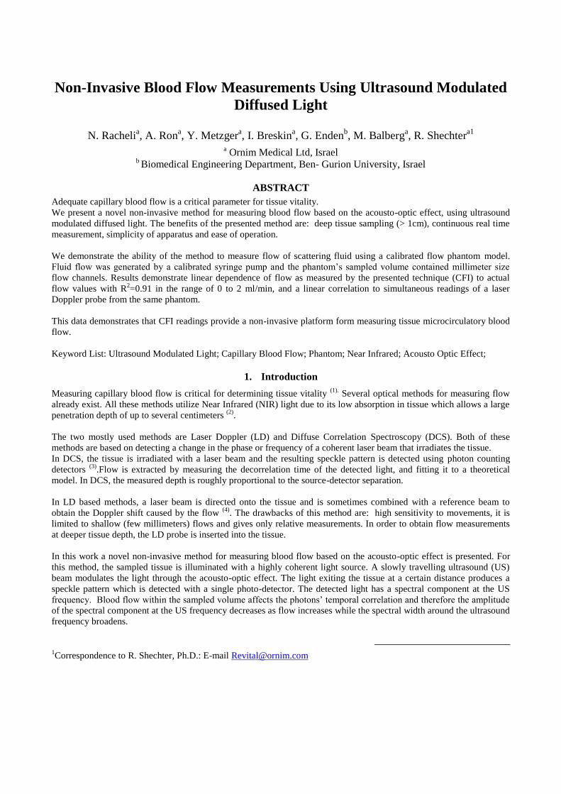
An example of a short train of US pulses introduced into the tissue is plotted in Figure 1A .This US train modulates the
light as it travels through the different medium layers. The measured light intensity by the detector is of the form shown
in Figure 1B. The time-based cross correlation between the US pulse train and detected light provides a depth profile of
the tagged light intensity which corresponds to a cross section of the ”banana” (for a given speed of sound in the
medium) as shown in Figure 1C. We denote this resulting profile a “UTL curve” (Ultrasound Tagged Light curve).
Figure 1 – a) The transmitted pulse train. B) The detected light intensity I(t) averaged over 10,000 traces.
c) The temporal cross correlation between the transmitted US sequence and the detected light.
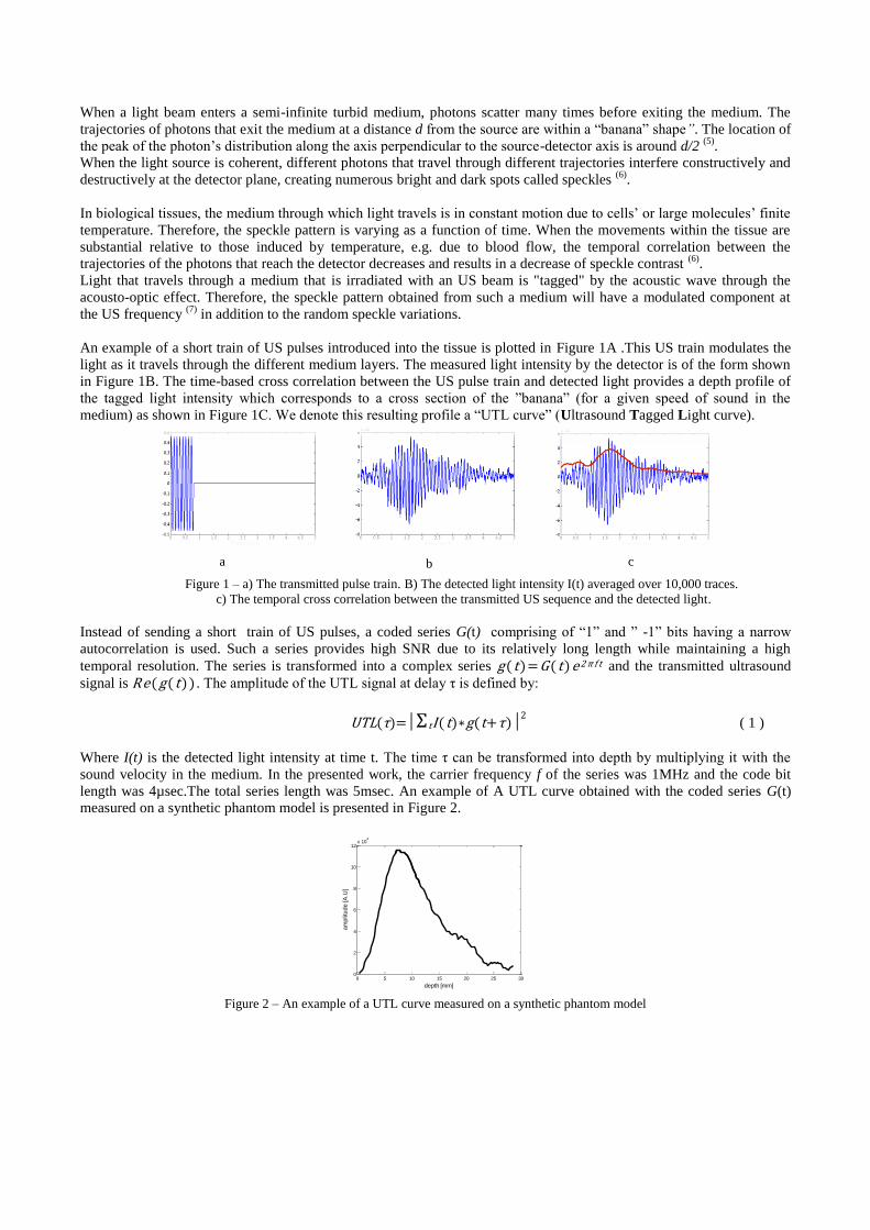
Instead of sending a short train of US pulses, a coded series G(t) comprising of “1” and ” -1” bits having a narrow
autocorrelation is used. Such a series provides high SNR due to its relatively long length while maintaining a high
temporal resolution. The series is transformed into a complex series g(t)=G (t)e2π f t and the transmitted ultrasound
signal is R e(g(t)) . The amplitude of the UTL signal at delay τ is defined by:
UTL(τ)=│ΣtI(t)∗g(t+τ)│2 ( 1 )
Where I(t) is the detected light intensity at time t. The time τ can be transformed into depth by multiplying it with the
sound velocity in the medium. In the presented work, the carrier frequency f of the series was 1MHz and the code bit
length was 4µsec.The total series length was 5msec. An example of A UTL curve obtained with the coded series G(t)
measured on a synthetic phantom model is presented in Figure 2.
Figure 2 – An example of a UTL curve measured on a synthetic phantom model
0 5 10 15 20 25 300
2
4
6
8
10
12x 10
4
depth [mm]
am
plitu
de
[A
.U]
a b c
As mentioned previously, the speckle contrast decreases proportionally to the motion of scatterers in the medium.
Therefore, the amplitude of the cross correlation between the US pulse and the intensity of the light, or the amplitude of
the UTL curve, is expected to decrease as flow increases.
2. Materials and methods
Experiments were performed on a tissue-mimicking phantom model in order to demonstrate the detection of changes in
flow using the proposed method. A tissue mimicking phantom that encapsulates millimeter size flow channels was
fabricated and the flow rate of scattering fluid was varied with a syringe pump. The experimental setup used for these
experiments is explained in detail in the following sections.
2.1. Tissue-mimicking Phantom structure
A phantom model that mimics blood flow in the tissue was designed. The phantom is made of UltraFlex (Douglas &
Sturgess Inc) which is a synthetic polymer matrix soaked with oil. TiO2 particles (0.1% by weight) were added as light
scattering agents. The optical and acoustic properties of the phantom are similar to those of tissue as listed in Table 1.
Table 1- optical and acoustic properties of the phantom and the tissue (2;11)
Property Tissue – muscle/brain Phantom
Light Effective decay coefficient 2.17/2.12 cm-1
2.2 ±0.2cm-1
Sound Velocity 1.5 ∙105 cm/s 1.43 ∙10
5 cm/s
Acoustic impedance 150-170 Kg/cm2s
149 Kg/cm
2s
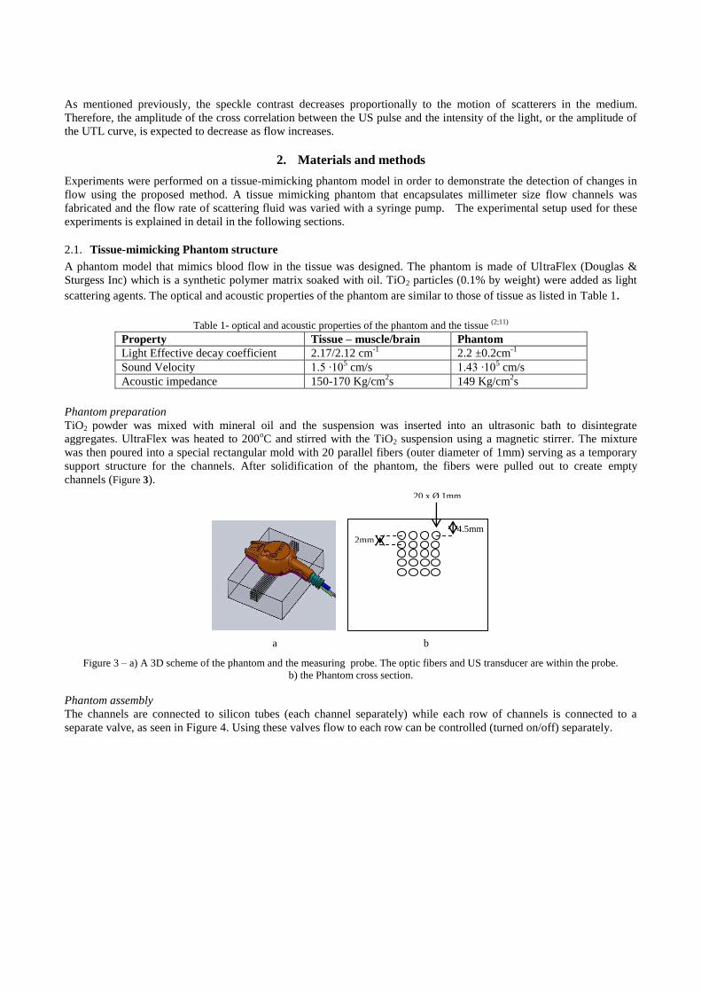
Phantom preparation
TiO2 powder was mixed with mineral oil and the suspension was inserted into an ultrasonic bath to disintegrate
aggregates. UltraFlex was heated to 200oC and stirred with the TiO2 suspension using a magnetic stirrer. The mixture
was then poured into a special rectangular mold with 20 parallel fibers (outer diameter of 1mm) serving as a temporary
support structure for the channels. After solidification of the phantom, the fibers were pulled out to create empty
channels (Figure 3).
Figure 3 – a) A 3D scheme of the phantom and the measuring probe. The optic fibers and US transducer are within the probe.
b) the Phantom cross section.
Phantom assembly
The channels are connected to silicon tubes (each channel separately) while each row of channels is connected to a
separate valve, as seen in Figure 4. Using these valves flow to each row can be controlled (turned on/off) separately.
2mm
4.5mm
20 x Ø 1mm
a b
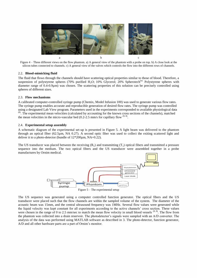
Figure 4 – Three different views on the flow phantom. a) A general view of the phantom with a probe on top. b) A close look at the
silicon tubes connected to channels. c) A general view of the valves which controls the flow into the different rows of channels.
2.2. Blood-mimicking fluid
The fluid that flows through the channels should have scattering optical properties similar to those of blood. Therefore, a
suspension of polystyrene spheres (70% purified H2O; 10% Glycerol; 20% SpherotechInc
Polystyrene spheres with
diameter range of 0.4-0.9µm) was chosen. The scattering properties of this solution can be precisely controlled using
spheres of different sizes.
2.3. Flow mechanisms
A calibrated computer-controlled syringe pump (Chemix, Model Infusion 100) was used to generate various flow rates.
The syringe pump enables accurate and reproducible generation of desired flow rates. The syringe pump was controlled
using a designated Lab View program. Parameters used in the experiments corresponded to available physiological data (8)
. The experimental mean velocities (calculated by accounting for the known cross sections of the channels), matched
the mean velocities in the micro-vascular bed (0.2-2.5 mm/s for capillary flow (9; 8)
.
2.4. Experimental setup assembly
A schematic diagram of the experimental set-up is presented in Figure 5. A light beam was delivered to the phantom
through an optical fiber (62.5µm, NA 0.27). A second optic fiber was used to collect the exiting scattered light and
deliver it to a photo-detector (bundle of 12*200µm, NA=0.22).
The US transducer was placed between the receiving (Rx) and transmitting (Tx) optical fibers and transmitted a pressure
sequence into the medium. The two optical fibers and the US transducer were assembled together in a probe
manufactures by Ornim medical.
Figure 5 – The experimental setup
The US sequence was generated using a computer controlled function generator. The optical fibers and the US
transducer were placed such that the flow channels are within the sampled volume of the system. The diameter of the
acoustic beam was 15mm, and the central ultrasound frequency was 1MHz. Several flow values were generated while
the liquid velocity was kept constant for all experiments according to the active channels’ cross section. These values
were chosen in the range of 0 to 2.5 mm/sec to match the mean flow velocity in small blood vessels (9; 8)
. The flow from
the phantom was collected into a drain reservoir. The photodetector’s signals were sampled with an A/D converter. The
analysis of the data was performed using MATLAB software as described in 3. The photo-detector, function generator,
A/D and all other hardware parts are a part of Ornim’s monitor.
a b c

2.5. Experimental procedure
Experiments were carried out with different flow rates. In each session a chosen flow rate was set and fluid flow was
kept constant for 2 minutes. Six experiments were performed to test the sensitivity to fluid flow in deeper channels. In
the first experiment all channels were activated. In the second experiment, the shallowest row of channels (4.5mm depth)
was activated and in the third experiment the central row of channels (8.5mm depth) was activated.
3. Data analysis and results
3.1. Extracting the Flow Index from the UTL curve
As a first step, the UTL curve (Figure 6) is normalized to the average light intensity (DC value) to account for the effect
of the light intensity on the amplitude of the cross correlation. Next, the Flow Index (CFI) is calculated from an interest
range k to k+N of the normalized UTL curved:
)
∗ ) )
( 2 )
where t is the discrete recording time.
Figure 6 – An example of a UTL curve. The solid line over the dashed UTL curve is the interest range from k to k+N
The chosen interest range is the range over which the UTL curve is most sensitive to flow variations. To find this range,
a linear regression between CFI and the real velocity rates was calculated for different interest ranges for the
configuration with all channels active. The interest range length (N) was chosen to be 5mm.
3.2. Experimental results
Experiments were performed with a sequence of ten flow rates in the range of 0 to 450 ml/min. The same sequence was
repeated while different channels were activated, as mentioned in section 2.5.
As expected, the amplitude of the UTL curves decreased as the flow rate through channel increased. In Figure 7 the
average UTL curves for different flow rates are presented. The most sensitive interest range was in the range of 8 to 13
mm. This interest range was used for all future CFI calculations.
0 5 10 15 20 25 300
2
4
6
8
10
12x 10
4
depth [mm]
am
plitu
de
[A
.U]
N
K
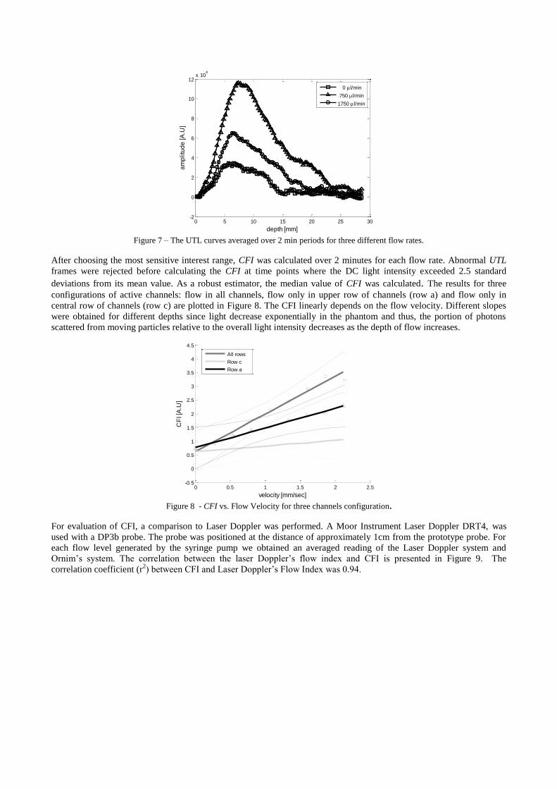
Figure 7 – The UTL curves averaged over 2 min periods for three different flow rates.
After choosing the most sensitive interest range, CFI was calculated over 2 minutes for each flow rate. Abnormal UTL
frames were rejected before calculating the CFI at time points where the DC light intensity exceeded 2.5 standard
deviations from its mean value. As a robust estimator, the median value of CFI was calculated. The results for three
configurations of active channels: flow in all channels, flow only in upper row of channels (row a) and flow only in
central row of channels (row c) are plotted in Figure 8. The CFI linearly depends on the flow velocity. Different slopes
were obtained for different depths since light decrease exponentially in the phantom and thus, the portion of photons
scattered from moving particles relative to the overall light intensity decreases as the depth of flow increases.
Figure 8 - CFI vs. Flow Velocity for three channels configuration.
For evaluation of CFI, a comparison to Laser Doppler was performed. A Moor Instrument Laser Doppler DRT4, was
used with a DP3b probe. The probe was positioned at the distance of approximately 1cm from the prototype probe. For
each flow level generated by the syringe pump we obtained an averaged reading of the Laser Doppler system and
Ornim’s system. The correlation between the laser Doppler’s flow index and CFI is presented in Figure 9. The
correlation coefficient (r2) between CFI and Laser Doppler’s Flow Index was 0.94.
0 5 10 15 20 25 30-2
0
2
4
6
8
10
12x 10
4
depth [mm]
am
plitu
de
[A
.U]
0 l/min
750 l/min
1750 l/min
0 0.5 1 1.5 2 2.5-0.5
0
0.5
1
1.5
2
2.5
3
3.5
4
4.5
velocity [mm/sec]
CF
I [A
.U]
All rows
Row c
Row a
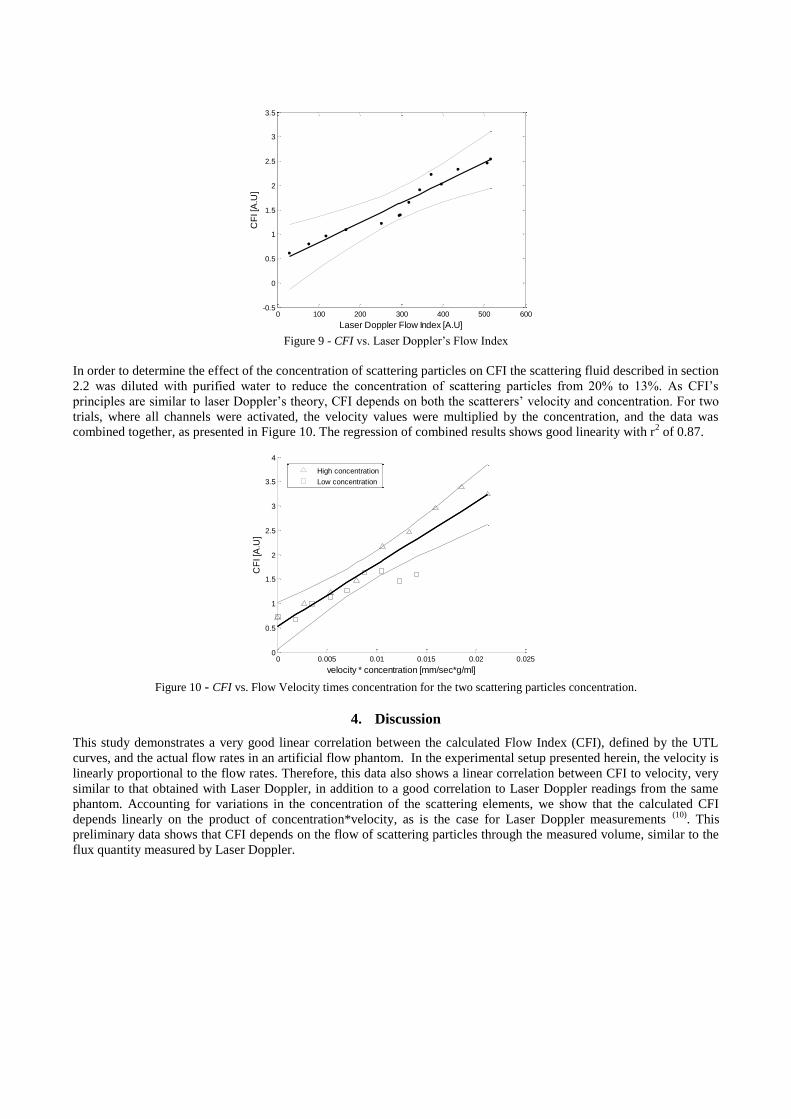
Figure 9 - CFI vs. Laser Doppler’s Flow Index
In order to determine the effect of the concentration of scattering particles on CFI the scattering fluid described in section
2.2 was diluted with purified water to reduce the concentration of scattering particles from 20% to 13%. As CFI’s
principles are similar to laser Doppler’s theory, CFI depends on both the scatterers’ velocity and concentration. For two
trials, where all channels were activated, the velocity values were multiplied by the concentration, and the data was
combined together, as presented in Figure 10. The regression of combined results shows good linearity with r2 of 0.87.
Figure 10 - CFI vs. Flow Velocity times concentration for the two scattering particles concentration.
4. Discussion
This study demonstrates a very good linear correlation between the calculated Flow Index (CFI), defined by the UTL
curves, and the actual flow rates in an artificial flow phantom. In the experimental setup presented herein, the velocity is
linearly proportional to the flow rates. Therefore, this data also shows a linear correlation between CFI to velocity, very
similar to that obtained with Laser Doppler, in addition to a good correlation to Laser Doppler readings from the same
phantom. Accounting for variations in the concentration of the scattering elements, we show that the calculated CFI
depends linearly on the product of concentration*velocity, as is the case for Laser Doppler measurements (10)
. This
preliminary data shows that CFI depends on the flow of scattering particles through the measured volume, similar to the
flux quantity measured by Laser Doppler.
0 100 200 300 400 500 600-0.5
0
0.5
1
1.5
2
2.5
3
3.5
Laser Doppler Flow Index [A.U]
CF
I [A
.U]
0 0.005 0.01 0.015 0.02 0.0250
0.5
1
1.5
2
2.5
3
3.5
4
velocity * concentration [mm/sec*g/ml]
CF
I [A
.U]
High concentration
Low concentration
The described experimental setup demonstrates the linear dependence of CFI on flow of scattering particles through the
channels, but is not used to calibrate the CFI dependence on flow in live tissue. This is due to the different decorrelation
time of the phantom’s solid matrix and due to the different coupling efficiency between the probe and the phantom
relative to those of tissue.
For clinical application CFI depends on several parameters, including the US coupling efficiency between the transducer
and the skin, the decorrelation time of the tissue and on the concentration of moving particles inside the measured
volume.
5. Conclusions
A novel method for continuously and non invasively measuring flow in deep tissue based on ultrasound modulated
diffused light is presented. The data demonstrates a linear correlation of CFI readings to flow rates in channels that are
deeper than 1cm in a synthetic phantom. The CFI readings are shown to depend on the concentration of scattering
centers within the channels. A very good correlation to Laser Doppler readings from the same phantom is also
demonstrated. CFI readings provide a non-invasive platform form measuring tissue microcirculatory blood flow.
6. Bibliography
1. Louis, Jean Vincent and De Backer, Daniel. “Microvascular dysfunction as a cause of organ dysfunction in severe
sepsis,” Critical Care , pp. s9-s12 (2005).
2. Welch, Ashley J., Prahl, Scott A. and Wai-Fung, Cheong. “A Review of the Optical Properties of Biological
Tissues,” IEEE Journal Of Quantum Electronics, VOL. 26. No. 12, December, pp. 2166-2185 (1990)
3. Cheung, Cecil, et al. “In vivo cerebrovascular measurement combining diffuse near-infrared absorption and
correlation spectroscopies,” Phys. Med. Biol. 46, pp. 2053–2065 (2001)
4. Fredriksson I., Fors C. and Johansson J., "Laser Doppler Flowmetry – a Theoretical Framework," Department of
Biomedical Engineering, Linköping University, www.imt.liu.se/bit/ldf/ldfmain.html (2007)
5. Guoqiang Yu, Turgut Durduran, Gwen Lech, Chao Zhou, Britton Chance, Emile R. Mohler III, and Arjun G.
Yodh, J. “Time-dependent blood flow and oxygenation in human skeletal muscles measured with noninvasive near-
infrared diffuse optical spectroscopie” Biomed. Opt. 10, 024027 (2005)
6. Yodh, Arjun G. and Boas, David A. “Spatially varying dynamical properties of turbid media probed with diffusing
temporal light correlation,” J. Opt. Soc. Am. A/ Vol. 14, No. 1/January, pp. 192-215 (1997)
7. Uzgiris, E., et al. “Ultrasonic tagging of light: Theory,” Applied Physical Sciences, Vol 95, pp. 14015-14019 (1998)
8. Guyton, Arthur C. and Hall, Jhon E. [Medical Physiology] Elsevier Health Sciences , pp. 150-158. (2005)
9. Schaller, B. “Physiology of cerebral venous blood flow: from experimental data in animals to normal function in
humans,” Brain Research Reviews 46, pp. 243-260. (2004)
10. Nilsson, E. Gert., Tenland, Torsten and Ake, P. Oberg. “Evaluation of a Laser Doppler Flowmeter for
Measurement of Tissue Blood Flow,” IEEE TRANSACTIONS ON BIOMEDICAL ENGINEERING, pp. 597-604.
(1980)
11. Christensen, Douglas A. [Ultrasonic Bioinstrumentation] Wiley , (1988)
Vital Signs for Vital Organs™
Non-Invasive Blood Flow Measurements Using
Ultrasound Modulated Diffused Light
N. Rachelia, A. Rona, Y. Metzgera, I. Breskina, G. Endenb, M. Balberga, R. Shechtera
a Ornim Medical Ltd, Israelb Biomedical Engineering Department, Ben- Gurion University, Israel
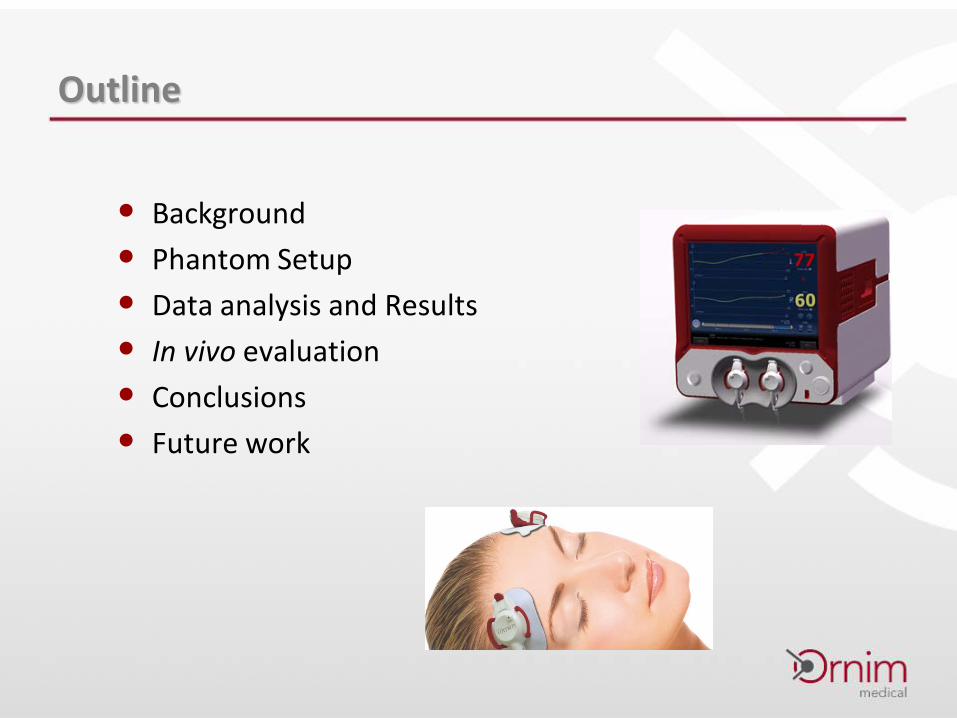
Outline
• Background• Phantom Setup• Data analysis and Results• In vivo evaluation • Conclusions• Future work
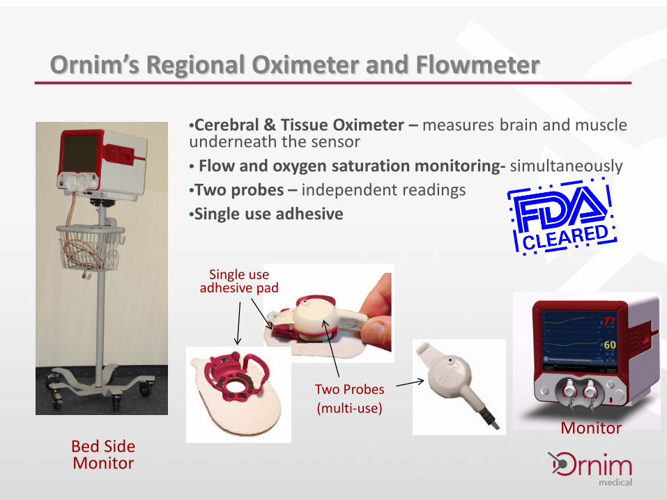
Ornim’s Regional Oximeter and Flowmeter
Monitor
Two Probes(multi-use)
Single use adhesive pad
Bed Side Monitor
•Cerebral & Tissue Oximeter – measures brain and muscle underneath the sensor• Flow and oxygen saturation monitoring- simultaneously•Two probes – independent readings•Single use adhesive
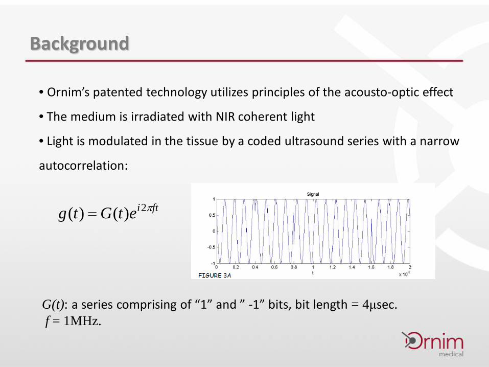
Background
• Ornim’s patented technology utilizes principles of the acousto-optic effect
• The medium is irradiated with NIR coherent light
• Light is modulated in the tissue by a coded ultrasound series with a narrow
autocorrelation:
ftietGtg π2)()( =
G(t): a series comprising of “1” and ” -1” bits, bit length = 4μsec. f = 1MHz.
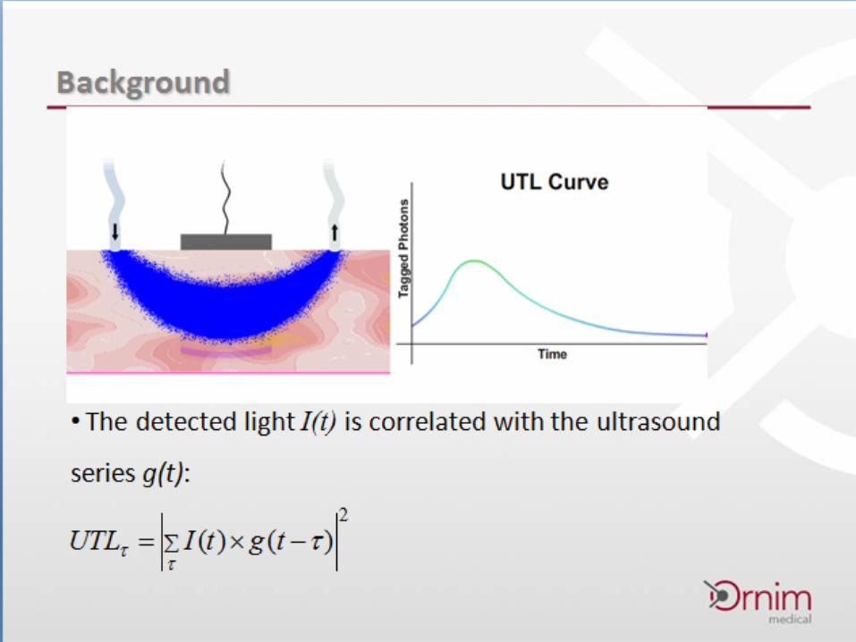
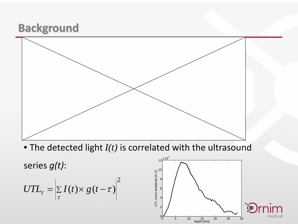
Background
• The detected light I(t) is correlated with the ultrasound
series g(t):2
)()(∑ −×=τ
τ τtgtIUTL
0 5 10 15 20 25 300
2
4
6
8
10
12 x 104
depth [mm]
UTL
cur
ve a
mpl
itude
[A.U
]
Background
• The detected light I(t) is correlated with the ultrasound
series g(t):2
)()(∑ −×=τ
τ τtgtIUTL
0 5 10 15 20 25 300
2
4
6
8
10
12 x 104
depth [mm]
UTL
cur
ve a
mpl
itude
[A.U
]
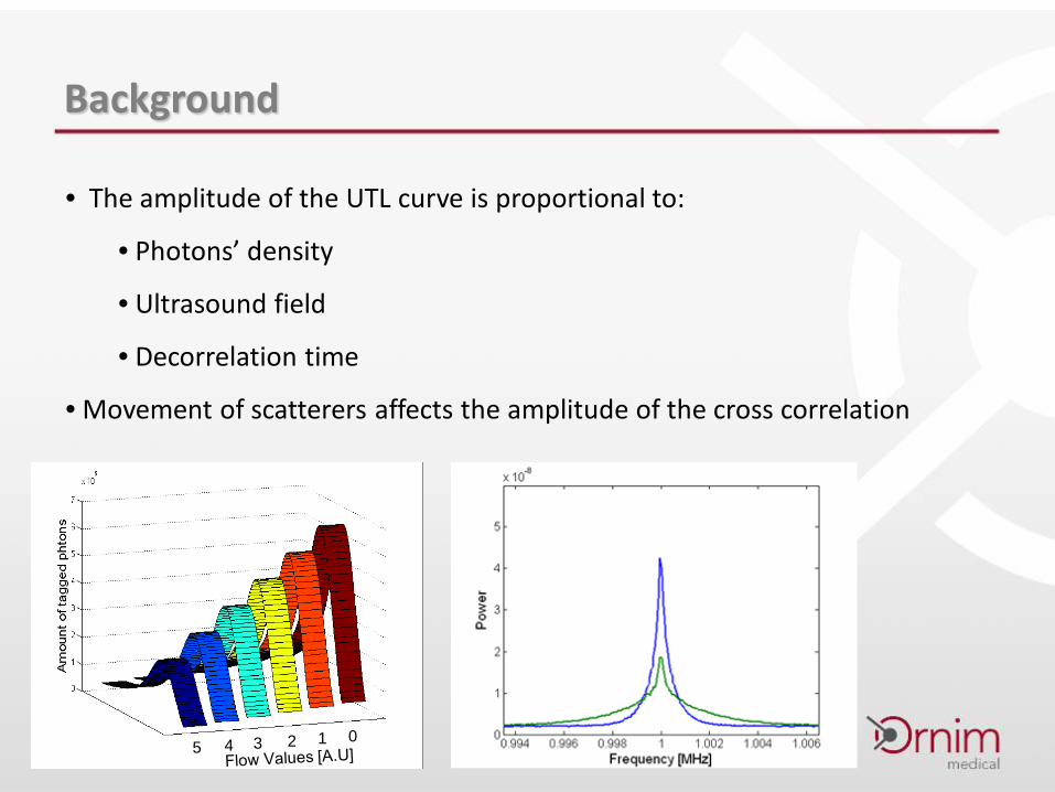
Background
• The amplitude of the UTL curve is proportional to:
• Photons’ density
• Ultrasound field
• Decorrelation time
• Movement of scatterers affects the amplitude of the cross correlation
2)()(∑ +×=
ττ τtgtIUTL
ftietGtg π2)()( =
012345

Experimental setup
Phantom1
Syringe pump2 Reservoir
Tissue mimicking phantom with micro channels simulates small blood vessels
1Generate flow at the range of 0 to 2.5 mm/sec
2Deliver coherent light and Ultrasound into the phantomRecord and analyze the light signal
3
3
Fluid:
70% purified H2O;10% Glycerol; 20% SpherotechInc Polystyrene spheres, 0.4-0.9µm (5% W/V)

Data Analysis and Results
• Extracting the Flow Index (CFI) from the UTL curve
1
)()(1)(
−+
=
×
= ∑Nk
kii tUTL
NtItCFI
0 5 10 15 20 25 300
2
4
6
8
10
12x 10
4
depth [mm]
UTL
cur
ve a
mpl
itude
[A.U
]
N
K
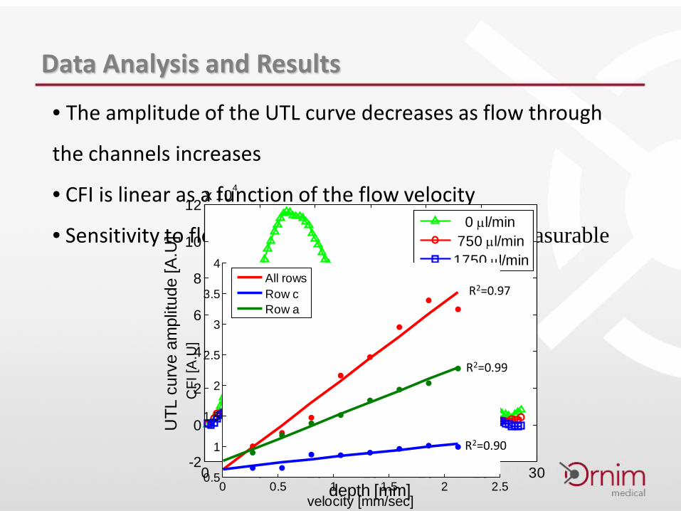
Data Analysis and Results
• The amplitude of the UTL curve decreases as flow through
the channels increases
• CFI is linear as a function of the flow velocity
• Sensitivity to flow in deep channels is lower but measurable
0 5 10 15 20 25 30-2
0
2
4
6
8
10
12x 104
depth [mm]
UTL
cur
ve a
mpl
itude
[A.U
]
0 µl/min 750 µl/min1750 µl/min
0 0.5 1 1.5 2 2.50.5
1
1.5
2
2.5
3
3.5
4
velocity [mm/sec]
CFI
[A.U
]
All rowsRow cRow a
R2=0.97
R2=0.99
R2=0.90

Data Analysis and Results
• The effect of scatterers concentration was tested
• Diluted the original liquid from 1% to 0.66% of Polystyrene spheres (W/V)
• The CFI is linear as a function of the normalized velocity values
0 0.005 0.01 0.015 0.02 0.0250
0.5
1
1.5
2
2.5
3
3.5
4
velocity * concentration [mm/sec*g/ml]
CFI
[A.U
]
High concentrationLow concentration
R2=0.87
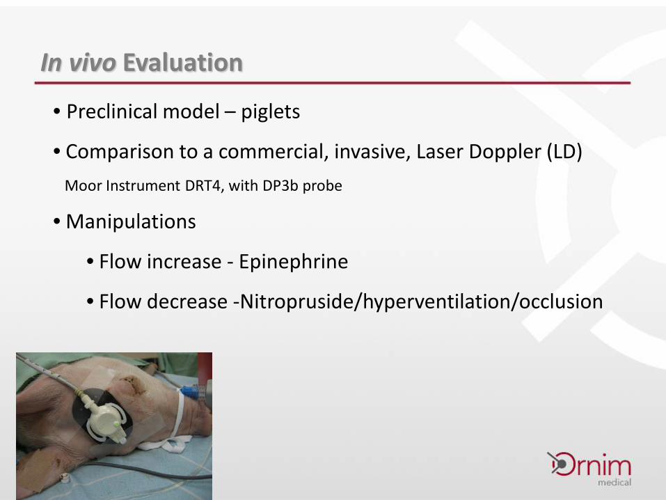
In vivo Evaluation
• Preclinical model – piglets
• Comparison to a commercial, invasive, Laser Doppler (LD)Moor Instrument DRT4, with DP3b probe
• Manipulations
• Flow increase - Epinephrine
• Flow decrease -Nitropruside/hyperventilation/occlusion
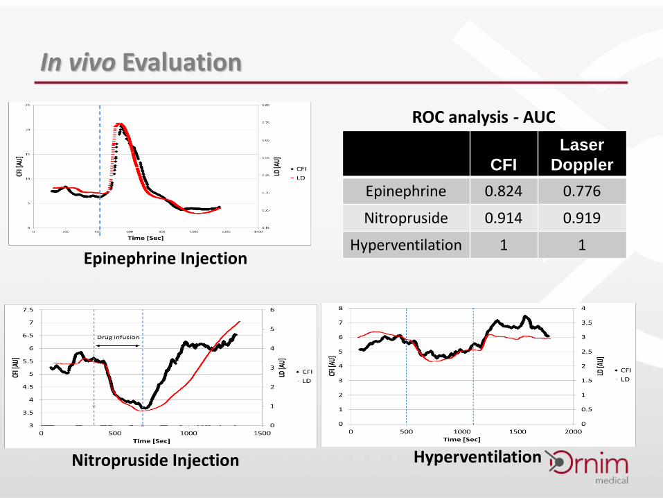
In vivo Evaluation
CFILaser
DopplerEpinephrine 0.824 0.776
Nitropruside 0.914 0.919
Hyperventilation 1 1Epinephrine Injection
Nitropruside Injection
ROC analysis - AUC
Hyperventilation
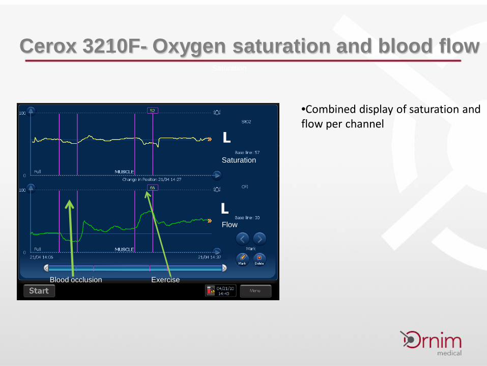
Cerox 3210F- Oxygen saturation and blood flow
•Combined display of saturation and flow per channel
Saturation
Flow
Blood occlusion Exercise
Saturation
Conclusions
• A novel method for continuously and non invasively measuring flow in deep tissue based on ultrasound modulated diffused light was presented
• Data demonstrates a linear correlation of CFI to flow in channels deeper than 1cm in a synthetic phantom
• A very good in vivo correlation to Laser Doppler readings was demonstrated
Future Work
• Clinical studies – cerebral flow monitoring during surgeries
• Calibrate CFI
• Numerical model

Vital Signs for Vital Organs™
THANK YOU
http://www.ornim.com
Vital Signs for Vital Organs™