University of South FloridaScholar Commons

Graduate Theses and Dissertations Graduate School

January 2013

Non-equilibrium melting and sublimation ofgraphene simulated with two interatomic potentialsBrad SteeleUniversity of South Florida, brad4@mail.usf.edu

Follow this and additional works at: http://scholarcommons.usf.edu/etd

Part of the Condensed Matter Physics Commons, and the Materials Science and EngineeringCommons

This Thesis is brought to you for free and open access by the Graduate School at Scholar Commons. It has been accepted for inclusion in GraduateTheses and Dissertations by an authorized administrator of Scholar Commons. For more information, please contact scholarcommons@usf.edu.

Scholar Commons CitationSteele, Brad, "Non-equilibrium melting and sublimation of graphene simulated with two interatomic potentials" (2013). GraduateTheses and Dissertations.http://scholarcommons.usf.edu/etd/4586

Non-equilibrium melting and sublimation of graphene simulated with two

interatomic potentials

by

Bradley A. Steele

A thesis submitted in partial fulllmentof the requirements for the degree of

Master of ScienceDepartment of Physics

College of Arts and SciencesUniversity of South Florida

Major Professor: Ivan I. Oleynik, Ph.D.Vasily V. Zhakhovsky, Ph.D.Inna Ponomareva, Ph.D.Sagar Pandit, Ph.D.

Date of Approval:March 20, 2013

Keywords: REBO, Molecular Dynamics, Stone Wales Defects, Double Vacancy,Single Vacancy, Liquid Carbon, Carbon Chains, Carbon Vapor, Condensation,

Coexistance, Maxwell Construction

Copyright c© 2013, Bradley A. Steele

Table of Contents

List of Figures . . . . . . . . . . . . . . . . . . . . . . . . . . . . . . . . . . . iii

Abstract . . . . . . . . . . . . . . . . . . . . . . . . . . . . . . . . . . . . . . iv

1 Introduction To Graphene . . . . . . . . . . . . . . . . . . . . . . . . . . . 11.1 Graphene as a Two Dimensional Wonder Material . . . . . . . . . . . . 11.2 Instability of Two Dimensional Crystals . . . . . . . . . . . . . . . . . 11.3 Melting by the Formation of Point Defects . . . . . . . . . . . . . . . . 21.4 Characterizing the Phase Transition at High Temperature . . . . . . . 3

2 Modeling the Phase Transition . . . . . . . . . . . . . . . . . . . . . . . . 42.1 Existing Models of the Melting Process . . . . . . . . . . . . . . . . . . 42.2 Using Molecular Dynamics to Model the Phase Transition . . . . . . . 5

3 Point Defects in Graphene . . . . . . . . . . . . . . . . . . . . . . . . . . 83.1 Stone Wales Defect and Vacancies . . . . . . . . . . . . . . . . . . . . 83.2 Activation and Formation Energies . . . . . . . . . . . . . . . . . . . . 9

4 Previous Experimental and Computational Results for the Melting of Grapheneand Graphite . . . . . . . . . . . . . . . . . . . . . . . . . . . . . . . . . . 114.1 Diculty in Determining the Melting Temperature Experimentally . . 114.2 Previous Computational Results . . . . . . . . . . . . . . . . . . . . . 14

5 Previous Studies on Liquid and Gaseous Carbon . . . . . . . . . . . . . . 175.1 Experimental Results . . . . . . . . . . . . . . . . . . . . . . . . . . . . 175.2 Computational Results . . . . . . . . . . . . . . . . . . . . . . . . . . . 18

6 Results on the Sublimation Process of Graphene . . . . . . . . . . . . . . 216.1 Computational Details: Sublimation . . . . . . . . . . . . . . . . . . . 216.2 Determination of the Sublimation Temperature . . . . . . . . . . . . . 21

6.2.1 Method for Finding Sublimation Temperature . . . . . . . . . . 216.2.2 Determination Using the REBO Potential . . . . . . . . . . . . . 246.2.3 Determination Using the SED-REBO Potential . . . . . . . . . . 25

6.3 Mechanisms of Sublimation . . . . . . . . . . . . . . . . . . . . . . . . 266.3.1 Mechanisms of Sublimation Using the REBO Potential . . . . . 266.3.2 Mechanisms of Sublimation Using the SED-REBO Potential . . 29

i

7 Results on Liquid and Gaseous Carbon . . . . . . . . . . . . . . . . . . . 327.1 Computational Details: Condensation . . . . . . . . . . . . . . . . . . 327.2 Sublimation and the Gas Phase of Carbon . . . . . . . . . . . . . . . . 337.3 Coexistance of the Liquid and Gaseous Phases . . . . . . . . . . . . . . 36

7.3.1 Description of the Coexistance Using the REBO Potential . . . . 367.3.2 Description of the Coexistance Using the SED-REBO Potential . 377.3.3 Comparison with Previous Results on Liquid Carbon . . . . . . . 40

8 Conclusion . . . . . . . . . . . . . . . . . . . . . . . . . . . . . . . . . . . 41

References . . . . . . . . . . . . . . . . . . . . . . . . . . . . . . . . . . . . . 42

ii

List of Figures

Figure 1 Evolution of the potential energy for dierent heating rates . . . . 22

Figure 2 Relationship between the extracted sublimation temperature/latentheat and the heating rate . . . . . . . . . . . . . . . . . . . . . . . 23

Figure 3 Sequence of snapshots of a 'seed of melt' forming in graphene using the

REBO potential in 3D . . . . . . . . . . . . . . . . . . . . . . . . . . 26

Figure 4 Relation between the number of non-hexagonal rings and the sublimation

point in graphene . . . . . . . . . . . . . . . . . . . . . . . . . . . . 27

Figure 5 Sequence of snapshots taken in 2D for the REBO potential . . . . 28

Figure 6 Sequence of snapshots of a 'seed of melt' forming in graphene takenusing the SED-REBO potential in 3D . . . . . . . . . . . . . . . . 29

Figure 7 Histogram of the number of atoms immediately proceeding the phasetransformation of graphene . . . . . . . . . . . . . . . . . . . . . . 33

Figure 8 Snapshots taken of liquid/gaseous carbon along the 6,000 K isotherm 34

Figure 9 Pressure, volume, and average coordination calculated along the6,000 K isotherm for liquid/gaseous carbon . . . . . . . . . . . . . 34

Figure 10 Mean square displacement for liquid and gaseous carbon of variousdensities . . . . . . . . . . . . . . . . . . . . . . . . . . . . . . . . . 35

Figure 11 The energy barrier for a one atom sp-to-sp2 transformation for theREBO potential and the SED-REBO potential . . . . . . . . . . . 38

Figure 12 Snapshot taken of the gas phase using the SED-REBO potential . 38

iii

Abstract

The mechanisms of the sublimation of graphene at zero pressure and the conden-

sation of carbon vapor is investigated by molecular dynamics (MD) simulations. The

interatomic interactions are described by the Reactive Empirical Bond Order poten-

tial (REBO). It is found that graphene sublimates at a temperature of 5,200 K ±100

K. At the onset of sublimation, defects that contain several pentagons and heptagons

will form, that are shown to evolve from double vacancies and SW defects. These

defects consisting of pentagons and heptagons will eventually form carbon chains.

The inuence of the interatomic interactions on the sublimation process are also in-

vestigated by comparing the results that are obtained using the REBO potential with

the screened environment dependent (SED)-REBO potential. Two-dimensional MD

simulations are also performed, and it is found that graphene melts at a much higher

temperature and forms many more point defects than in three dimensions. It is also

observed that carbon chains make up the two-dimensional molten state.

The isothermal equation of state of gaseous and liquid carbon, as well as the coex-

istance of the two phases is calculated at 6,000 K and up to a few GPa. The analysis

shows that the material that forms immediatly following the phase transformation in

graphene is actually a coexistance of liquid and gaseous phases, but it is primarily

two-fold coordinated, so it is mostly a gas, hence the identication of the phase trans-

formation as sublimation. The coexistance pressure for liquid and gaseous carbon is

found using the Maxwell Construction to be 0.0365 GPa at 6,000 K. At a pressure

lower than the coexistance pressure, carbon vapor undergoes a densication and de-

velops a small amount (∼6 %) of sp2 bonds. The diusion coecient of this dense

iv

gas is calculated to be in between that of the liquid and gaseous phases.

v

1 Introduction To Graphene

1.1 Graphene as a Two Dimensional Wonder Material

Graphene is a one atom thick layer of carbon atoms composed of planar sp2 bonds

arranged in a hexagonal pattern. It is considered the basic building block for all

other graphitic structures. It can be wrapped to form nanotubes, or it can be stacked

to form graphite [1]. It is a very interesting material due to its exceptional thermal,

mechanical, and electronic properties as well as its implications as a novel 2D material

[1, 2, 3, 4]. It has been estimated to have very high rigidity with an elastic modulus

in the TPa range [5], and very high electronic mobility with some estimates reaching

up to 100,000 cm2·V−1·s−1 [1]. For these reasons, graphene oers many potential

practical applications, especially in device physics. By introducing defects into the

crystal structure, the properties of graphene can be altered [6]. Precise control over

the properties of graphene would make the material much more suitable for real-world

applications. One way to introduce defects into graphene is simply by the application

of temperature. Due to the strong, planar, sp2 bonds in graphene high temperatures

are required to form defects.

1.2 Instability of Two Dimensional Crystals

Graphene, as well as any other two-dimensional crystal, was originally believed to

be thermodynamically unstable according to the well known Mermin-Wagner theorem

dating back to about 70 years ago, with renements made about 40 years ago [7]. The

theorem states that there is a divergent contribution of thermal uctuations at nite

1

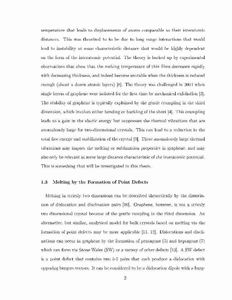
temperature that leads to displacements of atoms comparable to their interatomic

distances. This was theorized to to be due to long range interactions that would

lead to instability at some characteristic distance that would be highly dependent

on the form of the interatomic potential. The theory is backed up by experimental

observations that show that the melting temperature of thin lms decreases rapidly

with decreasing thickness, and indeed become unstable when the thickness is reduced

enough (about a dozen atomic layers) [8]. The theory was challenged in 2004 when

single layers of graphene were isolated for the rst time by mechanical exfoliation [2].

The stability of graphene is typically explained by the gentle crumpling in the third

dimension, which involves either bending or buckling of the sheet [4]. This crumpling

leads to a gain in the elastic energy but suppresses the thermal vibrations that are

anomalously large for two-dimensional crystals. This can lead to a reduction in the

total free energy and stabilization of the crystal [9]. These anomalously large thermal

vibrations may impact the melting or sublimation properties in graphene, and may

also only be relevant at some large distance characteristic of the interatomic potential.

This is something that will be investigated in this thesis.

1.3 Melting by the Formation of Point Defects

Melting in strictly two dimensions can be described theoretically by the dissocia-

tion of dislocation and disclination pairs [10]. Graphene, however, is not a strictly

two dimensional crystal because of the gentle rumpling in the third dimension. An

alternative, but similar, analytical model for bulk crystals based on melting via the

formation of point defects may be more applicable [11, 12]. Dislocations and discli-

nations can occur in graphene by the formation of pentagons (5) and heptagons (7)

which can form via Stone Wales (SW) or a variety of other defects [13]. A SW defect

is a point defect that contains two 5-7 pairs that each produce a dislocation with

opposing burgers vectors. It can be considered to be a dislocation dipole with a burg-

2

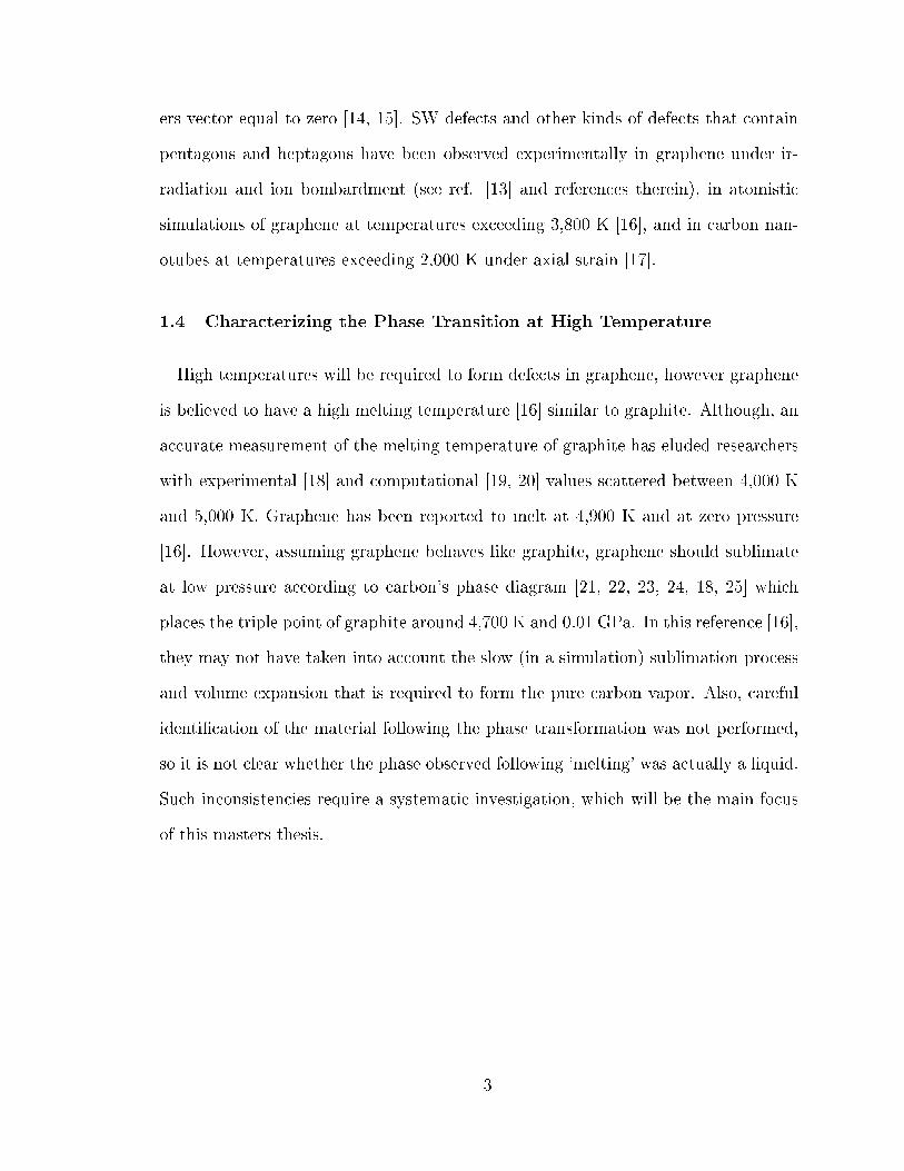
ers vector equal to zero [14, 15]. SW defects and other kinds of defects that contain

pentagons and heptagons have been observed experimentally in graphene under ir-

radiation and ion bombardment (see ref. [13] and references therein), in atomistic

simulations of graphene at temperatures exceeding 3,800 K [16], and in carbon nan-

otubes at temperatures exceeding 2,000 K under axial strain [17].

1.4 Characterizing the Phase Transition at High Temperature

High temperatures will be required to form defects in graphene, however graphene

is believed to have a high melting temperature [16] similar to graphite. Although, an

accurate measurement of the melting temperature of graphite has eluded researchers

with experimental [18] and computational [19, 20] values scattered between 4,000 K

and 5,000 K. Graphene has been reported to melt at 4,900 K and at zero pressure

[16]. However, assuming graphene behaves like graphite, graphene should sublimate

at low pressure according to carbon's phase diagram [21, 22, 23, 24, 18, 25] which

places the triple point of graphite around 4,700 K and 0.01 GPa. In this reference [16],

they may not have taken into account the slow (in a simulation) sublimation process

and volume expansion that is required to form the pure carbon vapor. Also, careful

identication of the material following the phase transformation was not performed,

so it is not clear whether the phase observed following 'melting' was actually a liquid.

Such inconsistencies require a systematic investigation, which will be the main focus

of this masters thesis.

3

2 Modeling the Phase Transition

2.1 Existing Models of the Melting Process

The oldest theory that explains the mechanism of melting comes from Lindemann

[26]. This simple model of melting is based on the vibrations of atoms. As the tem-

perature of the solid increases the average amplitude of the vibrations becomes larger

and eventually becomes comparable to interatomic distances. When this occurs the

atoms will begin to disturb their nearest neighbors and melting can occur. Since an

accurate quantitative calculation would be dicult, a simple relation for determining

the melting temperature based on the root mean vibration amplitude is given. As-

suming all the atoms vibrate with the same frequency, υE (Einstein approximation)

the average thermal vibrational energy can be related to the temperature using the

equipartition theorem, E = 4π2mυ2E < u2 >= kBT . Where < u >2 is the average

vibrational amplitude squared, T is the temperature, and m is the mass of the atom.

The lindemann criteria states that the melting will occur when < u >2= cla2 where cl

is the lindemann constant. In other words, melting occurs when the average thermal

vibrational amplitude becomes comparable to the interatomic distances. However,

experimental agreement is only fair [27].

This simple model obviously has its aws. For instance, it is based on a harmonic

model which does not allow for bond breaking or the formation of defects. In addition,

it is based on the assumption that the melting is homogeneous throughout the crystal.

Hence, this model can not take into account the observation of heterogeneous melting,

which involves the nucleation of the liquid phase at certain preferred sites in the solid

4

(the free surface, grain boundaries, large dislocations and disclinations, etc), followed

by subsequent growth of the liquid phase.

One such model that can account for such phenomena is based on the formation of

point defects by Stillinger and Weber who propose a simple statistical model [12]. It is

based on the idea that at the melting transition the amount of defects reaches a max-

imum. It also assumes that there exists, what they call, defect softening which causes

a softening of the solid that eases the formation of additional defects and introduces

new local modes of vibration. After minimizing the free energy with respect to the

number of defects, they obtain a temperature dependence of the number of defects,

which indeed does show a sharp peak at the melting temperature. Further develop-

ment of the theory includes eects due to interstitials, which allow for the calculation

of thermodynamic properties of the material in the solid, liquid, or amorphous state

[28]. A spike in the number of defects at the melting point has been observed in a sim-

ulation of the melting (it is described as melting in this paper, but this is inconsistent

with the phase diagram of carbon) of graphene in a recent paper by Zakharchenko

et. al (our results give similar qualitative agreement for sublimation) [16]. So despite

the fact that these models, which are based on the formation of point defects, were

created for bulk crystals, they do qualitatively give good agreement with simulations

of graphene. A similar model for a purely 2D system has also been developed [10] as

well as models for surface melting [29, 30].

2.2 Using Molecular Dynamics to Model the Phase Transition

We will be using Molecular Dynamics (MD) to study the sublimation process of

graphene. Our MD simulations are implemented in LAMMPS [31]. Describing the

interatomic interactions of graphene with a rst principles calculation such as density

functional theory (DFT) would be ideal to describe the sublimation process. However,

incorporating large system size and a large number of particles to model the melt-

5

ing/sublimation process makes DFT based MD computationally prohibitive. This

makes MD simulations employing empirical potentials a viable option. MD simula-

tions have been shown to reproduce the phase diagram of carbon within experimental

uncertainty [32]. MD also allows one to probe physical phenomena on time (on the

order of ps) and length scales (on the order of Å) much smaller than an experiment

can.

MD is based on Newtonian mechanics where each atomic position is updated ac-

cording to the initial position, initial velocity, and acceleration. Updating the position

at each step in the simulation can be performed according to the Verlet algorithm

[33]. The algorithm works as follows: at each time step the the potential is calculated

based on the positions of all the atoms, then the velocities are adjusted according

to the gradient of the potential, and nally each position is adjusted according to

the velocities. The validity of this method hinges on the quality of the interatomic

potential which usually involves several empirical parameters that are adjusted to

match sets of experimental results such as elastic constants, stress-strain curves, and

bond energies. Furthermore, the potential typically includes a cuto distance where

the potential begins to level o and the force is taken to be zero beyond this distance.

Longer range potentials extend this distance to more accurately match the binding

energy curves given by DFT at the cost of being more computationally expensive.

One of the potentials that will be used in this master thesis is the Reactive Empirical

Bond Order Potential (REBO) [34]. Bond order potentials not only contain a pair

wise interaction term between carbon atoms but also a bond order factor that includes

many body eects that take into account bond angles, dihedral angles, bond lengths,

and atomic coordination. REBO has been shown to give a good description elastic

properties, defect energies, and surface energies for graphite and diamond [34]. It

has been widely used to describe not only diamond and graphite but also carbon

nanotubes. The potential is very well suited to investigate the behavior of carbon

6

systems under normal conditions of temperature and pressure. It has been shown that

REBO reproduces the results of LCBOPII and density functional molecular dynamics

(DF-MD) for liquid carbon below 2 g·cm−3 [35, 36, 37]. Above this density (at 6,000

K) REBO gives an under-representation of sp3 bonds. Hence, this is the highest

density we use in our calculations.

We will compare the results of REBO with the newly developed Screened Envi-

ronment Dependent (SED) REBO potential [38]. SED-REBO is a modied REBO

potential, including long-range interactions and a screening function able to discrimi-

nate between the rst and farther nearest-neighbor. The potential is able to reproduce

the response of carbon materials under high compressive or tensile stress. The tech-

nical details regarding the potential can be found elsewhere [38]. Another potential

that we will compare our results with is called the Long Range Carbon Bond Order

Potential (LCBOPII). LCBOPII is a sophisticated bond order potential including

short, middle, and long range contributions to the carbon carbon interaction. It has

been shown to reproduce the formation energy for the Stone Wales defect and single

vacancies [39]. In addition, it has also been shown to give an accurate equation of

state and hybridization of the liquid state of carbon at high temperature and pres-

sure [39]. Accurately representing the composition and energetics of the liquid state

of carbon will be important in describing the phase transition, so the properties of

liquid and gaseous carbon will also be investigated with REBO and SED-REBO.

7

3 Point Defects in Graphene

3.1 Stone Wales Defect and Vacancies

The formation and aggregation of point defects will play a crucial role in the sub-

limation of graphene. At temperatures exceeding 4,000 K (kBT=0.34 eV), the ener-

getics of defects with activation/formation energies on a comparable scale will play

a signicant role in a simulation of the sublimation of graphene. This is why it is

useful to elucidate the structure and energetics of some of the more common defects

that are known to occur.

The most common point defects are the Stone Wales (SW) defect mentioned in

the introduction, single vacancies (SV), and double vacancies (DV). SW defects are

formed by a rotation of a carbon carbon bond by ninety degrees which results in

the formation of two pentagons and two heptagons (55-77). SV's are simply the

removal of one atom from the crystal which results in the formation of a pentagon

(5-atom) and a nine-atom defect after relaxation around the defect. DV's can result

in the formation of pentagons, heptagons, and octagons in various ways; the 5-8-5

(two pentagons on opposite sides of an octagon) defect is formed by the removal

of two neighboring atoms or the merger of two single vacancies, the 555-777 defect

is formed by the rotation of a bond in the 5-8-5 defect, and a 5555-6-7777 defect

is formed by the rotation of another bond in the 555-777 defect (see ref. [13] for

a pictorial representation of these defects and how they form). It is known that

non-hexagonal rings induce local Gaussian curvature in a graphene sheet. Pentagons

represent positive curvature and heptagons represent negative curvature, and an even

8

number of pentagons and heptagons typically cancels the local curvature. Although,

it has been shown that SW defects can induce small local deviations from the at

structure [40].

3.2 Activation and Formation Energies

The probability of forming a defect can be determined by the Arrhenius law which

is equal to a prefactor (proportional to the frequency at which atoms collide) multi-

plied by Exp[Ea/kBT ], where Ea is the activation energy to form the defect, kB is

the Boltzmann constant, and T is the temperature. In other words, the higher the

activation energy the less likely a defect is to form, while the higher the temperature

the more likely a defect is to form. Another important factor is the formation energy

of defects. The formation energy is the dierence between the energy of the initial

state and the nal state of the defect. So the activation energy is the energy barrier

the atoms must overcome to make the defect, while the formation energy represents

how much higher in energy the system is with the defect than without it. The dier-

ence between the activation energy and the formation energy represents the energy

barrier for the defect to heal itself (the reverse process of forming the defect).

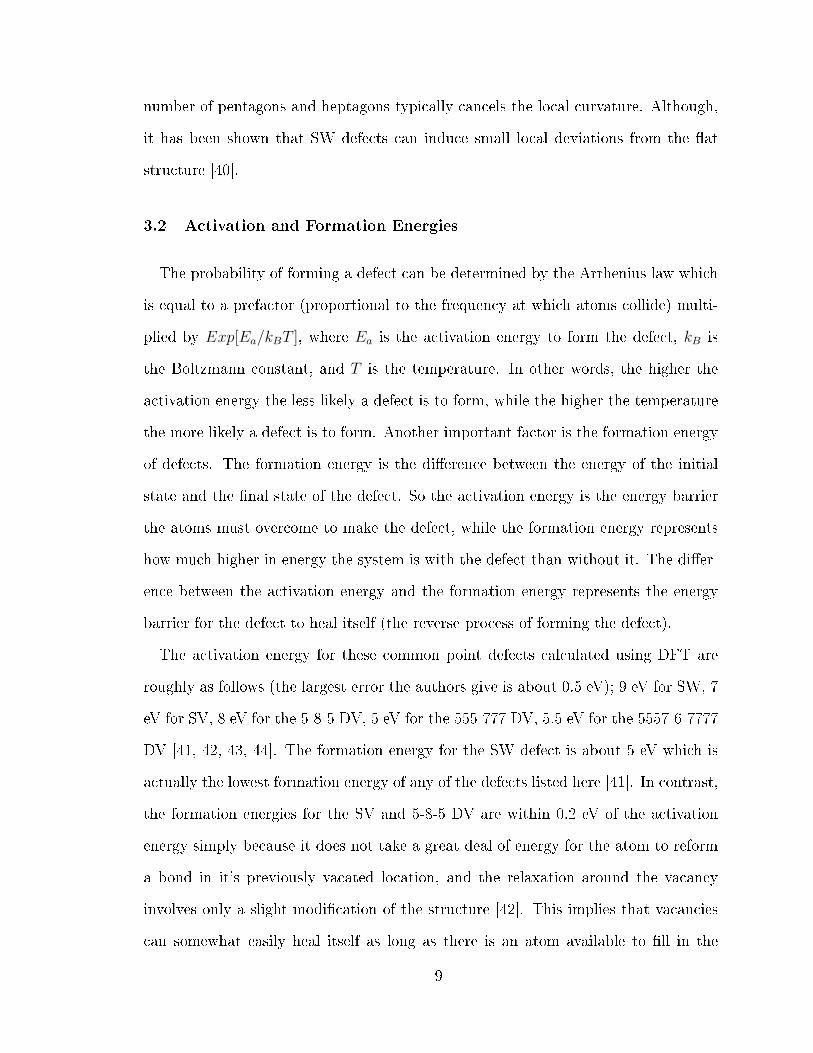
The activation energy for these common point defects calculated using DFT are

roughly as follows (the largest error the authors give is about 0.5 eV); 9 eV for SW, 7

eV for SV, 8 eV for the 5-8-5 DV, 5 eV for the 555-777 DV, 5.5 eV for the 5557-6-7777

DV [41, 42, 43, 44]. The formation energy for the SW defect is about 5 eV which is

actually the lowest formation energy of any of the defects listed here [41]. In contrast,

the formation energies for the SV and 5-8-5 DV are within 0.2 eV of the activation

energy simply because it does not take a great deal of energy for the atom to reform

a bond in it's previously vacated location, and the relaxation around the vacancy

involves only a slight modication of the structure [42]. This implies that vacancies

can somewhat easily heal itself as long as there is an atom available to ll in the

9

vacancy. On the other hand, the defects that involve a bond rotation are much more

stable because the reverse process takes much more energy which makes the SW, 555-

777 DV, and 5555-6-7777 DV fairly stable. Another important point to note is that

SV's have a small migration energy and can somewhat easily form the 5-8-5 DV via

the coalescence of two SV's with a calculated migration energy of only about 1 eV[42].

In other words, even though the SV's have the smallest activation energy (about 7

eV) migration and healing should cause this defect to be relatively unstable. Lastly,

the defects listed above are of course not the only kinds of defects that can form in

graphene. There are a myriad of other defects that can form via the coalescence of

multiple defects, multivacancies, and various bond rotations. Nonetheless, the defects

elucidated above are quite common in our simulations.

10

4 Previous Experimental and Computational Results for the Melting of

Graphene and Graphite

4.1 Diculty in Determining the Melting Temperature Experimentally

Graphene was not synthesized until 2004, and as of the current date of this mas-

ter thesis the author is not aware of any experimental melting lines measured for

graphene. However, the melting line for graphite has been studied extensively over

the past century. Since graphene's melting temperature is expected to be very similar

to graphite's it is useful to elucidate the results and the experimental diculties asso-

ciated with measuring the melting line for graphite. The experimental procedure for

measuring the melting line is fairly straightforward in concept [24, 45]. Essentially,

the tempereture of the sample is increased either through resistive heating or by laser

pulsed heating. At some point in time, the temperature will plateau indicative of

a phase transition. Afterwards, careful observation of the recrystallized material is

performed to determine whether the sample melted or sublimated. However, in prac-

tice, a number of issues prevent accurate measurements from being made for carbon.

This diers dramatically from the situation with metals, where the error is only a few

Kelvin.

One of the oldest experimental measurements on the melting temperature of graphite

was done by Pirani in 1930 [46]. In this work, graphite was melted by applying an

alternating current to rods with a blind whole drilled into the side surface. A py-

rometer was focused into these holes in order to measure the radiance and hence the

temperature of the sample. When the liquid lled this hole the radiance of the hole

changed abruptly, which was believed to coincide with the melting point. The author

11

applied this procedure successfully to measuring the melting point of several metals

at low pressure (0.1 MPa) with the expectation that it would yield adequate results

for graphite as well [46]. The author observed the bulging of what is now considered

to have been graphite, as can be seen from a gure of the bulging in the original

paper. The author measured the temperature of this bulged region to be about 3,700

K and assumed that this was the melting point. This measurement is considered to

be incorrect, and the bulging is now considered to be due to an increase in plasticity

of the rod.

Following Pirani's work, experimentalists had diculty in measuring the the melt-

ing temperature precisely due to the diculty in measuring the precise instant of

melting [18]. It wasn't until the pioneering work done by Bundy in 1963 that a reli-

able measurement of the melting point at high pressures was made (1-10 GPa) [45].

The measurement involved the discharging of an electrical current through the carbon

sample, which was contained inside of a high pressure apparatus. The melting point

was taken to be given by the beginning of the decrease in electrical resisitivity. Bundy

found the melting temperature to be 4,100 K at 0.9 GPa, a maximum of 4,600 K at

about 7 GPa, and decreases to about 4,100 K at 12.5 GPa [45]. Bundy's work is still

highly regarded, however many subsequent papers give conicting data.

A myriad of additional work has been devoted to measuring the melting point of

graphite, which varies between 4,000-5,000 K [22, 25, 47, 48, 49, 50, 51, 52, 53]. A thor-

ough compilation and review of the work up to 2003 was provided by Savvatimskiy[18].

In this paper it was found that several key factors contributed to the discrepancy be-

tween experiments; non-uniform heating of the sample, diculty in measuring the

temperature using the pyrometer, expansion of the gas following melting, and some

issues associated with laser pulsed heating. Anisotropy of the structure could give

rise to non-uniform heating of the substance. For example, it has been found that

in the case of pulsed electric heating there is drop in the electrical resistivity in the

12

initial stages of heating [50, 49]. However, when annealed at a temperature greater

than 3,000 K this drop does not occur, resulting in a low resistivity of 50µΩcm. Sav-

vatimskiy suggests verifying such a resisitivity prior to measuring the melting point.

Another possible cause of non-uniform heating can occur by using a graphite sample

with low initial density (less than 2 g·cm−3) because the low densities usually contain

initial disorder in the system as was veried in ref. [54]. This disorder can give rise

to signicant dierences in the resisitivity even over small distances.

Another issue has to do with the sublimation of graphite and the diculty in

measuring the temperature with the pyrometer. It was found that when the distance

between the graphite surface and the apparatus enclosing the sample was large enough

(greater than 12 mm), a visible glow of a coagulated vapor cloud would form about

1 mm above the surface [18]. This was veried by orienting the optical axis of the

pyrometer along the sample's surface. The temperature of the vapor was measured

to be 4,000 K, similar to the lower values for the melting temperature that were

previously measured. When the distance was reduced to 0.05-0.15 mm, transparency

of the vapor was ensured and the melting temperature was found to be 4,750 K which

was reproduced by other papers employing similar techniques [18]. This work utilized

a laser pulse to heat the sample and a pyrometer to measure how the temperature

of the substance changed with time. The melting point can be characterized by a

temperature plateau where the temperature stops increasing and levels o for a short

period of time, followed by a reduction in the temperature when the sample melts

or sublimates. Savvatimiskiy points out that it is not easy to obtain a temperature

plateau at the melting point. Two necessary conditions for obtaining the plateau are

given; uniformity of the heat ux over the heating spot and restricting the volume

above the surface of the graphite. The volume must be restricted so that the vapor

does not coagulate above the surface as previously discussed, as well as to prevent

energy release to the coagulated vapor, and to provide a thin transparent layer of

13

vapor. Savvatimskiy also points out that fast heating is preferable because it reduces

the amount of vapor that forms via sublimation of the sample.

Another source of uncertainty in measuring the melting point comes from the ob-

servation of the rise in the temperature at the temperature plateau [18]. Savvatimskiy

oer two possible explanations for this. First, it may be due to the rise in pressure

which would cause the melting point to rise as long as the pressures are not too high.

Vereshchagin measured the melting point of graphite to be 4,750 K at 300 MPa and

6,500 K at 4 GPa yielding a slope of, dP/dT≈2.1 MPa/K [48]. This is consistent

with Savvatimskiy's data which gives the beginning of melting at about 4,900 K and

the end at about 5,200 K. Using the slope of 2.1 MPa/K and an initial pressure of

500 MPa the nal pressure would be 1.1 GPa [18]. This matches closely with a cal-

culation that showed the pressure as a function of temperature and dierent layers of

the sample [18]. Second, it could also be due to surface melting which would cause

the top layer of graphite to melt early on in the melting time. The rest of the sample

would continue to melt, however parts of the surface layer may rise in temperature.

This is a known problem for metals with low conductivity, and the problem could be

amplied in graphite because of it's low conductivity in the 'c' direction [18].

Savvatimskiy concludes that some of the lower estimates for the melting point

between 3,700-4,000 K are unreliable, and that the majority of experimental studies

gives a melting point of graphite between 4,600-5,000 K at pressures above 10 MPa.

Graphene may have a similar melting point as graphite, but it would depend on how

the mechanisms that give rise to melting dier between the two materials.

4.2 Previous Computational Results

Simulations employing empirical potentials for carbon have previously been used

to study the mechanisms of melting of graphene and graphite. A recent Monte Carlo

simulation by Zakharchenko et al using LCBOPII has shown that graphene melts

14

via the formation of clusters of pentagons and heptagons that are reported to form

by way of clusters of SW defects [16]. This is followed by the formation of octagons

or larger rings, and nally the formation of carbon chains. This is in contrast to

graphite which melts via the formation of interplanar bonds. A similar process re-

sulting in the formation of carbon chains has also been observed in a simulation of

the melting of carbon nanotubes using a Terso potential [55] and in the melting

of fullerenes using the Brenner potential [56]. Zakharchenko found that the melting

temperature of graphene was 4,900 K which is close to the value obtained for nan-

otubes of 4,800 K [55]. In order to nd the melting temperature, Zakharchenko used

a modied lindemann criteria that averages over several nearest neighbor atoms. This

is needed because the ordinary lindemann criteria is divergent at nite temperatures

in 2D. They nd that melting occurs when this modied lindemann criteria is equal

to roughly 0.1 which is close to the lindemann criteria calculated for a strictly 2D

triangular lattice [57].

Zakharchenko's simulations were performed at zero pressure and the nal molten

state is reported to be a complex liquid phase composed of interconnected carbon

chains. However, assuming graphene behaves like graphite, graphene should subli-

mate at low pressure according to carbon's phase diagram [21, 22, 23, 24, 18, 25]

which places the triple point of graphite around 4,700 K and 0.01 GPa.

Nonetheless, a value of 4,900 K for the melting point is within the experimentally

acceptable range of melting temperatures of graphite. However, this is greater than

the value of 4,250 K at 2 GPa based on free energy calculations of graphite [19]. Free

energy calculations depend critically on the structure of the system and the interac-

tions between the particles. In ref. [19] an einstein crystal [58] is used to model the

solid phase and a lennard jones potential to model the liquid phase, parameterized

by LCBOPII. The parameterization was based on the rst two peaks of the radial

distribution function and the mean square displacement from equilibrium calculated

15

using LCBOPII. Both the radial distribution function and the equation of state used

to model the solid and liquid phases match up well with the results obtained with

LCBOPII. Verifying LCBOPII's predicted liquid phase as well as the melting mech-

anisms for graphene against other reliable potentials would therefore be useful.

LCBOPII gives a good estimation of the melting temperature when compared to

what is considered to be the most reliable experiments discussed in the previous

section. Nonetheless, the carbon chains that are observed with LCBOPII and the

Brenner potential are reminiscent of carbon chains that have been observed for uni-

axial strain of graphene. It is well known that REBO gives an over-representation

of carbon chains during uniaxial strain (see ref. [59] and references therein) due to

the spurious force that arises near the cuto distance. The cuto distance is typ-

ically adjusted for simulations that impose a large amount of strain to avoid these

erroneous results. It is natural to speculate whether the chains observed during the

melting could also be an artifact of the potential. It is fairly well established that

small carbon chains, Cn where 2<n<8, are the primary molecular species in carbon's

vapor phase [60, 61, 62]. However the chains that form during the melting process

are not in an equilibrium state so therefore warrant investigation.

16

5 Previous Studies on Liquid and Gaseous Carbon

5.1 Experimental Results

The melting/sublimation process of graphene obviously involves a transition to the

liquid/gaseous phase of carbon. This is why it is important for an MD interatomic

potential to not only accurately describe the structure and energetics of graphene,

but also the structure of liquid/gaseous carbon. One of the most well cited papers

investigating carbon vapor goes back to 1973 [60]. In this reference, experimental

data, including the carbon vapor pressure and specic heat, were t to empirical

functions based on the assumption that carbon vapor is composed of small carbon

chains (Cn n < 10). Coexistence curves between the gaseous and liquid phases are

also given that give fair agreement to experimental data [63]. Our results are also

in good agreement with this study at low pressure, however at higher pressure and

densities (well within the range that is studied) we nd that there is roughly 10 % sp2

bonds in a dense gaseous phase. This implies a slight non-chain bonding character.

There has been much more work done investigating liquid carbon. Prior to Bundy's

experiments in 1963, theoretical predictions of the heat of fusion based on the assump-

tion that the liquid phase of carbon at low pressure is composed of long molecular

chains gave a heat of fusion of, ∆H=0.44 eV/atom [18]. Bundy measured the heat

of fusion to be, ∆H=1.09 eV/atom [22]. This led Bundy to believe that the liquid

state of carbon is composed of smaller carbon chains. Later, more sophisticated ex-

periments gave a heat of fusion between 1-1.25 eV/atom [52, 64], close to Bundy's

results.

17

Since liquid carbon only exists in thermal equilibrium at high temperatures (about

6,000 K) it is dicult to probe it's structure experimentally. One interesting experi-

ment was performed by Johnson et. al in 2005 by laser pulsed heating of amorphous

carbon [65]. They measured the amount of π∗ states per site by time resolved x-

ray absorption spectroscopy. This indicates, roughly, the average coordination of the

sample. The coordination being the number of bonds that an atom has formed. For

example, in pristine graphene each atom has a coordination of 3 corresponding to

the sp2 hybridized orbitals. An sp3 bond has 0 π∗ states per site, an sp2 bond has

one π∗ state per site, and an sp bond has two. At a density of 2.0 g·cm−3 there were

on average 1.5 π∗ states per site and at 2.6 g·cm−3 there were 1.4 π∗ states per site.

This means that the liquid was composed of a combination of sp and sp2 hybridized

orbitals. The sp hybridized orbitals can be considered a carbon chain such as what

makes up carbon's vapor phase, however there are other structures that can be sp

hybridized. For example, a carbon chain that closes in on itself in a loop would be

entirely sp hybridized but would obviously have a dierent structure than a chain.

5.2 Computational Results

Johnson compared this result with a theoretical study that utilized a tight binding

model of carbon which gave good agreement, except at higher density where theory

may have over-predicted the coordination slightly [37]. A direct comparison with

experiment is also somewhat dicult to make because Johnson was unable to measure

the temperature and pressure of their samples in the experiment. Nonetheless, these

simulations showed that as the density was increased from 1.4-4.2 g·cm−3 at 6,000

K and 7,000 K liquid carbon transformed from being primarily 2-fold coordinated

to primarily 3-fold coordinated at about 2 g·cm−3, then to being primarily 4-fold

coordinated at about 3.6 g·cm−3 [37]. Several other papers have given similar results

[66, 21, 67, 35] utilizing rst principles and density functional based MD, however the

18

results are not identical. These results indicate simply that liquid carbon's structure

is complex and therefore dicult to describe theoretically. This is especially true

because of all the various hybridizations that have been shown to form simultaneously

in liquid carbon. It is therefore important to know how the structure/composition

of liquid carbon diers among various MD interatomic potentials to not only know

how accurate they are, but also as a way to aid in the characterization of the melting

mechanisms of graphitic structures.

There have been previous studies on how the REBO potential describes liquid

carbon. For example, a study that was done using the most recent version of the

REBO potential compared the structure of liquid carbon at high pressure between

REBO, a rened LCBOP [68], and a density functional molecular dynamics (DF-MD;

Car-Parrinello[69]) method [35]. It was found that along the 6,000 K isotherm up to

a pressure of about 60 GPa (6.5 Å3) they each give a very similar equation of state.

However, they each give dierent hybridizations. At a specic volume of about 7.2 Å3

REBO gave a mostly 2-fold coordinated liquid while both LCBOP and DF-MD gave

a mostly 3-fold coordinated liquid. Furthermore, at the smallest volume investigated,

5 Å3/atom, the REBO potential evolved to form a graphitelike liquid with almost

exclusively 3-fold coordinated atoms while both LCBOP and DF-MD both gave a

diamondlike liquid with mostly 4-fold coordinated atoms. LCBOP actually gave an

almost exclusively diamondlike liquid while the DF-MD contained about 62% of atoms

as 4-fold coordinated. The fact that LCBOP gives a result that is close to the DF-

MD result, which is more accurate, is surprising because LCBOP wasn't necessarily

developed to be used for liquid carbon especially at such high pressure.

The authors conclude that the long range interactions included in LCBOP and

the torsional energy term between 3-fold coordinated atoms plays a crucial role in

giving a good description of the liquid. The long range interactions were considered

to be important because of a simulation that was conducted on liquid carbon with

19

the short range version of LCBOP, called CBOP, reproduced the results of REBO

[68]. The authors point out that this is somewhat puzzling because the longer range

interactions are expected to be not as signicant at higher densities. The torsional

energy is considered signicant because it was previously shown that an older version

of REBO [70] gives a poor description of the torsional energy barrier and hence a poor

description of the liquid [66]. The discrepancy was that REBO gave a liquid-liquid

phase transition between a predominantly sp liquid to a predominantly sp3 liquid

which disagreed with the paper by Morris previously discussed (using tight binding)

and their rst principles MD results. Verication that the torsional barrier was the

cause of the problem was found by running simulations along the 6,000 K isotherm

with the torsional barrier, without the torsional barrier, and with 25% of the torsional

barrier. Neither with 25% of the barrier or without the barrier was a liquid-liquid

phase transition observed. A barrier strength of 25% was used because the calculated

energy versus torsional angle between two 3-fold coordinated bonded atoms was shown

to match rst principles calculations most accurately. This is justied because the

dependence on the angle is simply an empirical formula proportional to sin2Θ where

Θ is the torsional angle.

The potential we will be using will be the newer version of REBO which has this

correction. Also, at relatively low pressure and density REBO has been shown to

give good agreement with DFT and tight binding of liquid carbon up to a density of

2 g·cm−3 [36, 35]. The highest density we will use is about 2.00 g·cm−3 so we do not

anticipate any of the issues that we have discussed. Nonetheless, these results indicate

that the structure and atomistic hybridization of liquid carbon depends critically on

the analytical form of the potential.

20

6 Results on the Sublimation Process of Graphene

6.1 Computational Details: Sublimation

Sublimation simulations of free standing graphene are modeled using the MD code

implemented in LAMMPS [31] using periodic boundary conditions (PBC) at zero

pressure. Since the sublimation does not occur below 3,000 K, a substantial amount

of computational time is saved by equlibrating at 3,000 K initially, when a heating

rate is applied. In the two dimensional simulations, the system is relaxed at 6,000 K

prior to ramping the temperature because it is found that the melting temperature

is around 7,000 K in 2D. All simulations of graphene contain 12,960 atoms arranged

initially as a 200 X 185 Å2sheet. It was veried that the time step used, 4t = 0.2

fs, is small enough to maintain energy conservation at such high temperature. All

sublimation simulations are performed at constant pressure. Since graphene is a

two dimensional system, the pressure is controlled by allowing the simulation box

to expand in the x and y directions. For the transverse direction, the dimension is

chosen large enough to avoid the interaction of the sheet with itself through PBC.

6.2 Determination of the Sublimation Temperature

6.2.1 Method for Finding Sublimation Temperature

The sublimation temperature can be identied by where the Gibbs free energy for

the solid and gaseous phases are identical. At this temperature, energy is added to

the system to bring about the phase change, but the temperature and Gibbs free

energy do not change. However, when a heating rate is applied in a simulation,

21

Figure 1: Evolution of the potential energy for dierent heating rates (a). The tran-sition is characterized by a sharp change in the slope of potential energy.The sublimation temperature is estimated by tting a linear line to the PEbefore and during the transition, as shown for a=50 K/ps, and determiningthe intersection.

the temperature increases at a constant rate even when the system is undergoing

a phase transition, therefore the phase transition point will be overshot by some

amount depending on the heating rate. In order to account for this, the sublimation

temperature is found for graphene for smaller and smaller heating rates and then

extrapolated down to a heating rate of zero. The sublimation temperature for each

heating rate is determined by tting a straight line to the linear increase in potential

energy (PE) before sublimation and the (somewhat) linear increase in temperature

during sublimation shown in Figure 1. The sublimation temperature is determined by

the intersection point. The sublimation temperature vs. heating rate is then tted to

a square root function that gives a good t (Figure 2). In an experiment, the heating

rates would be much lower than in a MD simulation because MD can only simulate

up to a few ns, preventing experimentally realistic heating rates. Nevertheless, by

extrapolating to a heating rate of zero this can be taken into account and an accurate

determination for the sublimation temperature can be found.

A similar procedure for estimating the latent heat of sublimation is performed.

Straight lines are tted to the PE for the solid and non-equilibrium phases. The

non-equilibrium phase that forms after the sublimation process is not in equilibrium

22

Figure 2: Relationship between the extracted sublimation temperature (Ts) and thechange in enthalpy (4H) with the heating rate for graphene modeled bythe REBO potential in 3D. The method for acquiring the sublimation tem-perature and change in enthalpy is explained in the text.

because, at low pressure, it will expand to form a gas, but it takes a nite amount

of time for this to occur. Hence, it is referred to as a non-equilibrium dense gas

or liquid-like gas (discussed later on). The dierence between the two straight lines

tted to the energy before and after sublimation, at the sublimation temperature,

would be exactly equal to the change in internal energy of the system (the pressure is

equal to zero), at that heating rate, if the exact sublimation temperature and specic

heats were known (for our simulations). The errors in the tted lines are found to

be; ±100 K for the sublimation temperature, ±10−6 eV/atom·K for the slope in the

solid phase,±10−5 eV/atom·K for the slope in the gaseous phase, 10−4 eV/atom for

the intercept in the solid phase, and 10−3 eV/atom for the intercept in the gaseous

phase. Constant temperature simulations are also performed in order to obtain a more

accurate determination of the melting temperature. The temperature is chosen to be

the estimate obtained from the previous simulation as a starting point. The static

temperature simulations are more computationally expensive, especially when not

using the simple REBO potential, so only one relevant static temperature simulation

is performed with the SED-REBO potential.

23

6.2.2 Determination Using the REBO Potential

In Figure 1, a plot of the PE versus temperature for dierent heating rates is

shown that is used to estimate the sublimation temperature. Using the method

described previously, the sublimation temperatures that are obtained, from the largest

heating rate to the smallest are: 6,100 K, 5,900 K, 5,800 K, and 5,500 K. By visual

inspection of the slow increase in energy around the extracted sublimation point, the

error for these measurements is determined to be ±100 K. The extracted sublimation

temperature versus heating rate is plotted in Figure 2. Although it does not converge

for the heating rates used, an estimate of the sublimation temperature at a heating

rate of zero can be made. The t results in a sublimation temperature of 5,300 K.

This t is expected to overestimate the sublimation temperature because the tted

curve is above the measured sublimation temperature at the two smallest heating

rates and due to the lack of convergence at small rates.

In order to conrm these results, constant temperature simulations are performed at

5,100 K and 5,200 K. Since the sublimation process is a slow process for temperatures

close to the actual sublimation temperature, the constant temperature simulations are

run for over a nanosecond. It is found that graphene sublimates at 5,200 K after about

600 ps, while at 5,100 K sublimation does not occur even after 1,200 ps. On this time

scale it is reasonable to conclude that the sublimation temperature is 5,200 K for

REBO with an error of roughly ±100 K. This is close to the sublimation temperature

of 4,900 K obtained by Zakharchenko et al. [16] using LCBOPII. It is also within the

error (±100 K) of the sublimation temperature obtained just by using the t.

In the two dimensional simulations, a similar procedure is conducted and it is found

that the melting temperature is 7,000 K±100 K. Similarly to the 3D case, constant

temperature simulations are conducted at zero pressure at 6,900 K and 7,000 K for

800 ps. It is found that melting occurs at 7,000 K, but not at 6,900 K.

The latent heat of sublimation of graphene is extrapolated to a heating rate of

24

zero to be 1.38 ± 0.03 eV/atom in 3D (Figure 2). The error is calculated using

the estimated errors for the melting temperature, slopes, and intercepts given in the

previous section. A value of 1.38 eV/atom is only slightly larger than the values

obtained by Bundy for the melting heat of graphite which range between 0.7-1.3

eV/atom [45], which was subsequently rened to be about 1.25 eV/atom [18]. Since

Bundy's experiment measured the melting of graphite, as opposed to the sublimation,

it would seem as though the non-equilibrium dense gas phase that forms following the

sublimation of graphene is similar to molten graphite. This non-equilibrium dense-

gas phase will be discussed in more detail later on. In two dimensions, the carbon

atoms can not break their bonds as easily because they can not move into the third

dimension. Hence, the latent heat required to melt/sublimate the 3D system should

be more than the latent heat to melt the 2D system. Consistent with this idea, it is

found that the latent heat for a 2D system is approximately 0.98 eV/atom, about 0.4

eV smaller than sublimation in 3D.

6.2.3 Determination Using the SED-REBO Potential

For the SED-REBO potential, simulations with a heating rate of 3 K/ps, 12.5 K/ps,

and 50 K/ps are run and the corresponding sublimation temperatures are found to be,

4,600 K, 4,900 K, and 5,500 K respectively. By plotting the sublimation temperature

versus the heating rate similar to what was done with the REBO potential, the t

results in a sublimation temperature of 4,400 ± 200 K. The error is larger than for

the REBO potential because there are fewer data points. To verify this value and to

reduce computational time only one NPT simulation at zero pressure and at 4,300

K is conducted to verify the accuracy of the tting procedure. The PE does begin

to drift after about 200 ps indicating the onset of sublimation. We conclude that

the non-equilibrium sublimation temperature is 4,300 K ± 200 K for the SED-REBO

potential. This number is within the range of experimentally measured sublimation

25

temperature's of graphite [22].

6.3 Mechanisms of Sublimation

6.3.1 Mechanisms of Sublimation Using the REBO Potential

a db5

5

55

8

7

7

c

Figure 3: Sequence of snapshots of a 'seed of melt' that forms in graphene using the REBO

potential in the NPT ensemble taken at 5,400 K in 3D. Here, the process begins

by the merger of a SW defect and a DV (a), followed by a cluster of 5 and 7

atom defects (b) (55555-6-77777), then the initial chain formation (c), and nally

(d) shows a typical structure during the onset of sublimation with long chains

and defects surrounding the broken area. This melted/sublimated area will then

spread through the rest of the sheet. Time elapsed for each gure: 99 ps, 108 ps,

111 ps, and 120 ps respectively. Color scheme (# of atoms in ring): dark blue

(6), orange (5), light blue (7), yellow (8), and red (9).

Our description of the sublimation process using the REBO potential is very similar

to the melting process described by Zakharchenko using LCBOPII [16], except DV's

are a much more important part of the process. The DV's that are observed are

not only the 5-8-5 DV but also the 555-777 and 5555-6-7777 DV. In addition, the

structure shown in Figure 3(b) is observed. This structure contains 5 pentagons, 5

heptagons, and one hexagon in the center (55555-6-77777). This structure forms by

the merger of a SW defect and a DV (Figure 3(a)). The sequence of snapshots shown

in Figure 3(a-c) track the same piece of graphene.

The formation energy for DV's is about 3-4 eV less than the formation energy for

SW defects for pristine graphene [13]. In Figure 4, it is shown that the number of

octagons is near zero and the number of heptagons is much higher before the phase

transformation begins to occur, consistent with a much higher formation energy for

DV's than SW defects. However, as the phase transformation occurs, the number of

26

Figure 4: Relation between the number of non-hexagonal rings and the sublimation point

in graphene. The number of non-hexagonal rings increases exponentiallyas graphene undergoes the phase transformation. The number of octagonsstarts out near zero indicating almost no DV's, but as the system begins toundergo the phase transformation many more DV's are created. This sim-ulation was done with constant temperature at 5,400 K and zero pressure.

non-hexagonal rings increases exponentially and many octagons begin to form. The

DV in Figure 3(a) forms after 99 ps, which is very close to the point in time where

the potential energy begins to rise (Figure 4). About 10 ps later, breakdown of the

graphene sheet and the formation of the carbon chains can be seen (Figure 3(c)). In

summary, DV's are indeed an important part of the sublimation process despite their

high formation energy in pristine graphene.

Defects such as that shown in Figure 3(b) containing pentagons and heptagons

typically form the 'seed of melt' for graphene, which is where the sheet will begin

sublimating by rst forming the carbon chains and eventually the gas. This trans-

formation occurs despite the fact that this particular structure does not introduce

any curvature into the system because there are an even number of pentagons and

heptagons. The carbon chains can be seen to form in Figure 3(c),(d). Once the chains

form, the sublimated area spreads through the rest of the sheet until the whole sheet

has sublimated, however there can be multiple seeds of melt. This process for the sub-

limation is similar qualitatively with a model of melting based on the correspondence

27

ba c5

5

5

5

5

5

6

77

7

7

7

7 66

6

6

6 6

Figure 5: Sequence of snapshots taken in 2D for the REBO potential in the NPT en-semble at 7,400 K with 12,960 atoms. In (a) a ring-like structure containingalternating 5 and 7 atom defects is observed, followed by (b) where smallchains have begun to form in the plane as well as many 5 and 7 atom de-fects. In (c) melting is underway containing a few small chains interspersedin the plain of the sheet. Figure (c) has been shifted down by ∼ 5Å and tothe left ∼ 10 Å to see the chains more clearly. Time elapsed for each gure:

56 ps, 70 ps, and 87 ps respectively.

between the melting point and the aggregation and maximization of point defects

[12, 10, 28].

An in depth analysis of the migration of defects is not performed, however inspec-

tion of the snapshots during the sublimation process shows that the defects do not

appear to be very mobile. We see that the defects will disappear often. This is typi-

cally because the defects will heal themselves, however the evolution of most defects

are tracked on the order of ps, so the disappearance could be due to migration if the

migration occurs on a much smaller time scale.

The sublimation process for REBO in 2D follows the same pattern as in 3D; a seed

of melt will form that involves the formation of pentagons and heptagons, the carbon

chains will then form from the seed, and nally the seed/carbon chains will spread to

the rest of the sheet. The key dierence is that the defects begin to form at a much

greater temperature than in 3D. A common structure that is typically part of the

seed of melt is shown in Figure 5(a), the full seed of melt contains many 5 and 7 atom

defects similar to what can be seen around the edges of Figure 5(b). The structure in

5(a) is a called a 'ower' defect and it has been observed by chemical vapor deposition

on Ni but not on Cu [71] as well as by epitaxial growth on SiC(0001)[15]. It is only

28

natural to attribute defects like these to SW defects or a merger of SW defects. This

is because it is highly unplausible that any defects could be formed by vacancies since

the atoms do not have the extra degree of motion to migrate into. It is interesting

to note that the chains will form in the plane as part of the melting process in 2D as

shown in Figure 5(b),(c).

SW defects have a formation energy that is about twice as much when the rotation

is restricted to be in the plane [13], so it is not surprising that the SW defects form at

a much greater temperature in 2D. This is why the melting temperature is so much

higher in 2D. The chains require a certain amount of defects in the system in order to

form, and since vacancies are essentially forbidden, SW defects and SW-like defects

(that involve a bond rotation) are all that remain. Since these defects require a very

high temperature to form it makes sense the melting temperature is very high as well.

6.3.2 Mechanisms of Sublimation Using the SED-REBO Potential

a b c

Figure 6: Sequence of snapshots of a 'seed of melt' forming in graphene taken usingthe SED-REBO potential in 3D in the NPT ensemble at 4,800 K and with12,960 atoms. The immediate formation of a small chain is found (a) by therotation of a carbon carbon bond similar to the way a SW defect is formed.This quickly results in the formation of a relatively unstable defect other than a

SW defect (b). This structure did not form via a vacancy (there are no atoms

added or subtracted from the image except possibly for the atoms at the edges).

Eventually, this leads to the formation of chains and many uncoordinated atoms

at the onset of melting (c). Time elapsed for each gure: 20 ps, 21 ps, and 36 ps

respectively.

The sublimation mechanisms predicted by the SED-REBO potential are much dif-

ferent than REBO. It does not require many defects to cluster together, in contrast

29

to what was found previously. Instead, it usually involves the formation of broken

or dangling bonds as well as a small number of defects to initially form the 'seed of

melt'. As can be seen in Figure 6(a), two uncoordinated atoms and what can be con-

sidered a carbon chain forms in the sheet. This structure forms without any defects

previously present. The chain forms in the same way as a SW defect would form,

yet the SW defect does not form. Instead, this structure very quickly (less than a

ps) evolves into a defect containing four pentagons, two heptagons, and one hexagon

shown in Figure 6(b) by the rearrangement of atoms. The structure in Figure 6(b)

has the same number of pentagons as a SW defect and a 5-8-5 DV, but the structure

is dierent than if the two were isolated. This structure does introduce curvature into

the system because of the additional pentagons that are present and the deformation

of the sheet in the transverse direction is visible in the image. This structure seems

unstable because it is not observed often in our simulations. It is displayed here

simply to illustrate that the defect in Figure 6(a) does not form a SW defect.

Although it is not pictured, the formation of 5-8-5 double vacancies and SW defects

is occasionally observed, but at a much smaller concentration. Oddly the 555-777 DV

and the 5555-6-7777 DV is not observed (the activation energy of the 555-777 DV is

about 5 eV compared to about 7 eV for the 5-8-5 DV [42, 13]). This could be the

result of the activation energy for the chains to form from the 5-8-5 DV being less

than the activation energy for 555-777 DV to form. This would cause the chains to

be more likely to form instead of the 555-777 DV, and since the chains appear to be

preferred with the SED-REBO potential, this seems plausible. The reason why the

sublimation temperature is so much lower than what is predicted for REBO is this

apparent low activation energy for the chain structures. The clustering of defects that

would form the 'seed of melt' in for REBO requires a large concentration of defects

which requires high temperature. Since these kinds of defects are not required in

large concentrations in order for chains to form with the SED-REBO potential, the

30

sublimation temperature will be less than REBO. This is because the chains are what

ultimately cause the sheet to sublimate and are what makes up the gaseous phase.

31

7 Results on Liquid and Gaseous Carbon

7.1 Computational Details: Condensation

To recover the liquid phase following the melting of graphene that was reported

by Zakharchenko [16], and, more importantly, to indentify whether or not the non-

equilibrium material following the phase transformation of graphene is a liquid or

a gas, the carbon vapor is compressed into liquid carbon. The equilibrium carbon

vapor is easily identied as it contains many small non-interacting carbon chains and

has been previously studied [60], however the material that forms immediatly after

the phase transformation of graphene is more dense than pure carbon vapor and so

it may not be a gas as one would anticipate.

The pure carbon vapor is obtained from the sublimated graphene material, so it

contains an identical number of atoms as in the graphene simulations. The equilibrium

carbon vapor is relaxed dynamically for over a ns to achieve equilibrium in the NPT

ensemble (constant pressure). To sample the equation of state, the temperature

is xed at 6,000 K and the isotherm is calculated in the pressure range of 0.008-8

GPa. The volume is increased slowly such that the pressure changes by about 0.006

GPa at low pressure (< 0.15 GPa) and 0.15 GPa for higher pressure (> 0.15 GPa)

because the compressability changes dramatically at high pressure. Each simulation

is relaxed dynamically in the NVT ensemble at the specied volume for at least

300 ps. Simulations of the coexistance between liquid and gaseous phases require

more time to reach equilibrium, so they were relaxed for an additional 300 ps. Each

simulation uses the nal structure from the previous simulation as initial coordinates.

32

Figure 7: A histogram of the number of atoms along the transverse direction imme-diately proceeding the melting of graphene. The density is non-uniform,however in the central region where the density varies the least (between -5Å and 10 Å) the density is 0.25 g·cm−3 (specic volume of 80.16 Å

3) with

an average coordination of two. The average coordination at this densityand temperature nearly matches up with the data in Figure 9, and is at avolume/pressure less/greater than the coexistance point that is found forthe liquid and the gaseous phases.

The pure liquid and gaseous carbon reach equilibrium in about 20 ps. To obtain

thermal properties an average over the last 100 ps of the simulation is taken. It also

is important to point out that longe range Van der Waals forces are not included in

the potential.

7.2 Sublimation and the Gas Phase of Carbon

As mentioned previously, when the graphene sheet melts it transforms into a non-

equilibrium state. A histogram of the number of atoms along the transverse direction

of this non-equilibrium state has a Gaussian shape, indicating a non-uniform density

(Figure 7). Nonetheless, the average density in the central region where the density

varies the least, which contains roughly 65% of all the atoms, is about 0.25 g·cm−3

(specic volume of 80.16 Å3/atom) at 5,400 K and with an average coordination

of two. An average coordination of two at this specic volume and temperature (a

temperature dierence of 600 K is assumed to have a negligible eect) matches up

33

b ca d

Figure 8: Snapshots taken of liquid/gaseous carbon along the 6,000 K isotherm us-ing the REBO potential relaxed for at least 300 ps at (a) 0.015 GPa and852.4 Å

3/atom, (b) 0.033 GPa and 204.2 Å

3/atom, (c) 0.045 GPa and 66.4

Å3/atom, (d) 0.12 GPa, and 15.4 Å

3/atom. Figure (a) is the vapor phase

of carbon composed of many small chains. Upon compression, the vaporbecomes more dense (Figure (b)) and forms a small number of sp2 bonds(5.7 %), even though the coexistance point has not been reached yet. Fig-ure (c) shows the coexistance of the liquid and gaseous phases where theliquid is beginning to nucleate. Figure (d) is the pure liquid phase of carboncomposed of many sp2 bonds. The color scheme is the same as in Figure 3,except chains are the same color as hexagons (dark blue) in these gures.

a

b

Figure 9: Pressure, volume, and average coordination calculated along the 6,000K isotherm for liquid/gaseous carbon. Two ideal gas curves are shownthat have a reduced density as described in the text. The dilute carbonvapor is well described by the ideal gas curve, but the dense carbon vaporis not, indicating attractive forces between carbon chain molecules. Thecoexistance point between liquid and gaseous phases is about 0.0365 GPaand 160 Å

3/atom, which is found using the Maxwell Construction.

34

Figure 10: Mean square displacement (MSD) calculated using the REBO potentialfor various densities of liquid and gaseous carbon at 6,000 K. The slope ofthe line is proportional to the diusion constant. The dense carbon vapor(0.094 g·cm−3) has a diusion coecient that is roughly in between thatof the pure liquid and gaseous phases.

with the data in Figure 9, and is at a volume less than the coexistance point is found

to occur. This phase slowly expands, and after about 400 ps the pure equilibrium

carbon vapor is formed. The equilibrium carbon vapor consists of many small carbon

chains, Cn where n ranges from 1 to 31 (the average chain length is about 7) (Figure

8(a)) . This representation of gaseous carbon is similar to what has been previously

studied [60].

The equation of state for the pure carbon vapor is well-described by a modied ideal

gas law (at low pressure) which uses a reduced density of carbon chain molecules (as

opposed to singe carbon atoms) (Figure 9). The total number of chains is calcu-

lated using the program polypy which uses Franzblau statistics to calculate the total

number of chains [72]. However, the program considers a chain to be at least 3 con-

nected two-fold coordinated atoms so it does not count the amount of Cn, where n<5.

Nonetheless, it is calculated that 77.1% of atoms are apart of Cn, with n≥5, at 6,000

K and 0.008 GPa using the REBO potential. Only a small fraction of atoms, 1.5%

(at low pressure), are apart of loops which are carbon chains with the two end atoms

bonded to one another. For simplicity, it is assumed that the rest of the atoms are

35

evenly distributed between C2,C3, and C4 for the reference ideal gas curves.

The dilute ideal gas curve in Figure 9 is based on the carbon chain density given

by the dilute carbon vapor with specic volume 852.4 Å3/atom, and the dense ideal

gas curve is based on the carbon chain density given by the dense carbon vapor with

specic volume 61.8 Å3/atom. These ideal gas curves represent the kinetic portion

of the given pressure. The agreement at high specic volume (pressures below about

0.025 GPa) indicate almost no interactions between carbon chain molecules, and the

disagreement at higher pressure indicates attractive forces between the molecules.

These attractive forces cause a densication of the carbon vapor (with a structure

similar to that shown in Figure 8(b)) and give it liquid-like properties. For example,

at 204.2 Å3/atom (0.033 GPa), there is about 6 % sp2 bonds despite being mostly

chain-like (the liquid typically contains sp2 bonds [66, 19]). The presence of sp2

bonds indicates a slight non-chain bonding character that diers from the typical

representation of carbon vapor [60]. In addition, the self diusion coecient of the

dense gas is in between the values found for the gas and the liquid (Figure 10). The

self diusion coecient is calculated using the mean square displacement, which is

shown in Figure 10. The diusion coecient is found to be; 12.79 X 10−4 cm2s−1,

7.45 X 10−4 cm2s−1, 4.32 X 10−4 cm2s−1, and 1.52 X 10−4 cm2s−1 for specic volumes

852.4 Å3/atom, 204.2 Å

3/atom, 61.8 Å

3/atom, and 14.7 Å

3/atom respectively.

7.3 Coexistance of the Liquid and Gaseous Phases

7.3.1 Description of the Coexistance Using the REBO Potential

The coexistance point between the liquid and gaseous phases can be found by where

the Gibbs free energy for both phases are equal, or equivalently by when the change

in the Gibbs free energy is zero. The Gibbs free energy can be calculated with the

integral of the volume respect to pressure. This leads to the well-known Maxwell

equal-area Construction for nding the phase coexistance point described in most

36

statistical mechanics textbooks [73]. The coexistance point is found by integrating

the volume with respect to the pressure around the coexistance point, such that the

integral is equal to zero. The Maxwell Construction is performed using the data

shown in Figure 9, and the integral is calculated numerically. At a pressure of 0.0350

GPa and 0.0375 GPa the change in Gibbs free energy is a positive and negative value

respectively, implying that the coexistance point is in between these two pressures.

At 0.0365 GPa the change in the Gibbs free energy is equal to 1.45 X 10−4 eV/atom,

a relatively small value. Hence, 0.0365 GPa (160 Å3/atom) is the pressure that we

nd for the coexistance point between gaseous and liquid phases using the REBO

potential.

The non-equilibrium phase immediatly proceeding the phase transformation of

graphene previously discussed had a density of 80.16 Å3/atom. This means that

this material is a coexistance of liquid and gaseous phases. A snapshot of the coex-

istance of the two phases is shown in Figure 8(c) at 66.4 Å3/atom. This snapshot

has an average coordination of 2.07 which means that this material is still made up

of mostly chains. This means that this material is still mostly gaseous, whereas at

higher pressure the average coordination jumps (Figure 9(b)) as many sp2 bonds are

formed. This means that the material immediatly following the phase transforma-

tion of graphene is a coexistance of liquid and gas, but is mostly gas, hence the

identication of the phase tranformation as sublimation.

7.3.2 Description of the Coexistance Using the SED-REBO Potential

The energy barrier as two carbon chains (C9) are brought closer together until the

formation of two sp2 bonds for both potentials is shown in Figure 11 (Van der Waals

attraction is not included in both REBO and the SED-REBO potential). The barrier

is calculated by holding the two central carbon atoms xed followed by a conjugate

gradient energy minimization. The distance between the two central atoms changes

37

Figure 11: The energy barrier for a one atom sp-to-sp2 transformation for the REBOpotential and the SED-REBO potential. The Van der Waals attractiveforce is not included in either potential. The energy barrier is much greaterfor the SED-REBO potential reaching a maximum of about 3 eV, whilethe barrier for the REBO potential reaches a maximum of only 0.7 eV.Snapshots are shown of the initial state consisting of two non-interactingcarbon chains and the state with the lowest energy with an sp2 bond at aseparation of 1.45 Å. The relative potential energy (y-axis) is the dierencein potential energy between each point and the initial non-interacting chainenergy for that particular potential.

Figure 12: Snapshot taken using the the SED-REBO potential of the gaseous phase

relaxed in the NVT ensemble at 6,000 K and 2 GPa (23.5 Å3/atom).

This phase contains almost exclusively carbon chains, but is at a higherpressure than the REBO potential with the same average coordination(Figure 8(b)). This phase also has more chains (75 % of atoms) than it'sREBO counterpart (63.6 % of atoms). The color scheme is the same as inFigure 8.

38

at each point by 0.01 Å. Both carbon chains are initially linear and at ninety degrees

to one another as shown in the inset (on the right) in Figure 11. When the sp2 bond

forms, the chains bend so that the bonds are roughly at 120o to one another, as

would be expected (the inset on the left). The energy barrier for this transformation

is much greater for the SED-REBO potential than for the REBO potential by about

2.3 eV. Overcoming this barrier causes the amount of sp2 bonds in the gaseous phase

described by the SED-REBO potential to be very small (Figure 9(b)). The barrier

also completely prevents the condensation from occuring, as can be seen in Figure

9. Instead, a gas phase of repulsize carbon chains forms (Figure 12). This image is

at a specic volume of 23.5 Å3/atom, but is similar in appearence and has the same

average coordination as REBO does at 204.2 Å3/atom.

It is likely that the SED-REBO potential does not give a good description of the

liquid phase of carbon because of the large barrier that exists between carbon chains.

It is also possible that the sp-to-sp2 transformation portrayed in Figure 11 is not the

actual reaction pathway for sp2 bonds to form that occurs in DF-MD and experiment

[65, 66]. Nonetheless, there is useful information that can be extracted from this data.

The size of the barrier is relatively small for such high temperatures (about 3 eV for

SED-REBO and 0.7 eV for REBO), but this barrier is still enough to prevent the

condensation of the gas in SED-REBO. This must be due to the interaction between

many chains as the material becomes increasingly more dense. This would cause

the repulsive forces between the chains to accumulate, which is what prevents the

condensation. Hence, it is clear that the interaction between chains, such as what is

portrayed in Figure 11, plays a critical role in accurately describing the liquid phase

of carbon.

39

7.3.3 Comparison with Previous Results on Liquid Carbon

Good agreement with previous simulations done on liquid carbon is obtained with

the REBO potential but not with the SED-REBO potential. The general transition

from being primarily sp bonded to being primarily sp2 bonded has been reported

previously [37, 66, 21]. Wu et. al. obtained an average coordination of 2.60 at 1.27

g·cm−3 (at 6,000 K) using rst principles DF-MD [66], while an average coordination

of 2.52 at a density of 1.30 g·cm−3 (at 6,000 K and a pressure of 0.12 GPa) is found

using the REBO potential. In contrast, SED-REBO has an average coordination

of 2.13 at a density of 1.36 g·cm−3 indicating poor agreement. Another interesting

comparison can be made to an experiment done aimed at obtaining liquid carbon

by Johnson et. al. in which a femtosecond laser pump is used and time resolved

x-ray absorption spectroscopy is performed. Roughly an identical amount of 1 and 2

coordinated atoms is measured in their untamped run as the carbon vapor simulated

in this master thesis, which consists of about 70 % 2-fold coordinated atoms and 30

% 1-fold coordinated atoms [65].

40

8 Conclusion

In summary, the sublimation mechanisms of graphene using the widely known

REBO potential and the newly developed SED-REBO potential have been described

and the coexistance point has been found. Atomistic simulations show that graphene

sublimates by rst forming DV's and SW defects which results in the formation of

clusters of pentagons and heptagons. These clusters evolve into carbon chains that

eventually form a non-equilibrium dense gas phase of carbon. This dense gas phase

will continue to expand at low pressure on the order of hundreds of picoseconds

until equilibrium is reached. The sublimation process described by the SED-REBO

potential, begins with the creation of small carbon chains and large rings in the

graphene sheet. These large rings weaken the graphene sheet and allow the formation

of carbon chains. Our simulations show that the melting temperature is much higher

in 2-dimensional simulations simply due to the higher SW formation energy. Also,

it was found that the molten state in two dimensions also consists of mostly carbon

chains.

We have shown that carbon vapor, initially composed of non-interacting carbon

chains, forms a dense gas of attactive carbon chains at about 0.03 GPa and 6,000 K.

This dense gas phase is found to have a small sp2 fraction of atoms indicative of a

slight non-chain bonding character. The coexistence point is found to occur at about

0.0365 GPa (160 Å3/atom). It was found that the material that forms immediatly

proceeding the phase transformation of graphene is a coexistance of liquid and gaseous

phases, however is composed of mostly carbon chains indicating that it is mostlly gas.

41

References

[1] A. K. Geim and K. S. Novoselov, The rise of graphene., Nature materials,

vol. 6, pp. 18391, Mar. 2007.

[2] K. S. Novoselov, A. K. Geim, S. V. Morozov, D. Jiang, Y. Zhang, S. V. Dubonos,

I. V. Grigorieva, and A. A. Firsov, Electric eld eect in atomically thin carbon

lms., Science (New York, N.Y.), vol. 306, pp. 6669, Oct. 2004.

[3] K. S. Novoselov, A. K. Geim, S. V. Morozov, D. Jiang, M. I. Katsnelson, I. V.

Grigorieva, S. V. Dubonos, and A. A. Firsov, Two-dimensional gas of massless

Dirac fermions in graphene., Nature, vol. 438, pp. 197200, Nov. 2005.

[4] J. C. Meyer, A. K. Geim, M. I. Katsnelson, K. S. Novoselov, T. J. Booth, and

S. Roth, The structure of suspended graphene sheets., Nature, vol. 446, pp. 60

3, Mar. 2007.

[5] B. Yakobson, C. Brabec, and J. Berhnolc, Nanomechanics of carbon tubes:

Instabilities beyond linear response., Physical Review Letters, vol. 76, pp. 2511

2514, Apr. 1996.

[6] J. Lahiri, Y. Lin, P. Bozkurt, I. I. Oleynik, and M. Batzill, An extended defect in

graphene as a metallic wire, Nature Nanotechnology, vol. 5, no. 5, pp. 326329,

2010.

[7] D. Mermin, Crystalline Order in Two Dimensions, Phys. Rev., vol. 176, no. 1,

1968.

42

[8] J. A. Venables, G. D. T. Spiller, and M. Hanbucken, Nucleation and growth of

thin lms, Rep. Prog. Phys., vol. 47, pp. 399459, 1984.

[9] D. Nelson, T. Piran, and S. Weinberg, Statistical Mechanics of Membranes and

Surfaces. Singapore: World Scientic, 2nd ed., 2004.

[10] B. I. Halperin and D. R. Nelson, Theory of Two-Dimensional Melting, vol. 41,

no. 2, pp. 121124, 1978.

[11] D. Kuhlmann-yvilsdorf, Theory of Melting, Phys. Rev., vol. 140, no. 5A, 1965.

[12] F. H. Stillinger and T. A. Weber, Point defects in bcc crystals: Structures,

transition kinetics, and melting implications, The Journal of Chemical Physics,

vol. 81, no. 11, p. 5095, 1984.

[13] F. Banhart, J. Kotakoski, and A. V. Krasheninnikov, Structural defects in

graphene., ACS nano, vol. 5, pp. 2641, Jan. 2011.

[14] J. Hirth, J. P. and Lothe, Theory of Dislocations. McGraw-Hill, 1968.

[15] E. Cockayne, G. Rutter, N. Guisinger, J. Crain, P. First, and J. Stroscio, Grain

boundary loops in graphene, Physical Review B, vol. 83, p. 195425, May 2011.

[16] K. V. Zakharchenko, A. Fasolino, J. H. Los, and M. I. Katsnelson, Melting of

graphene: from two to one dimension., Journal of physics. Condensed matter,

vol. 23, p. 202202, May 2011.

[17] M. Nardelli, B. Yakobson, and J. Bernholc, Brittle and Ductile Behavior in

Carbon Nanotubes, Physical Review Letters, vol. 81, pp. 46564659, Nov. 1998.

[18] A. Savvatimskiy, Measurements of the melting point of graphite and the prop-

erties of liquid carbon (a review for 1963-2003), Carbon, vol. 43, pp. 11151142,

May 2005.

43

[19] F. Colonna, J. Los, a. Fasolino, and E. Meijer, Properties of graphite at melt-

ing from multilayer thermodynamic integration, Physical Review B, vol. 80,

p. 134103, Oct. 2009.

[20] G. Galli, R. M. Martin, R. Car, and M. Parrinello, Ab initio calculation of

properties of carbon in the amorphous and liquid states, Phys Rev B, vol. 42,

no. 12, 1990.

[21] M. Grumbach and R. Martin, Phase diagram of carbon at high pressures and

temperatures., Physical review. B, Condensed matter, vol. 54, pp. 1573015741,

Dec. 1996.

[22] F. Bundy, W. Basset, M. Wenthers, R. Hemley, H. Mao, and A. Goncharov, The

pressure-temperature phase and transformation diagram for carbon; updated

through 1994, Carbon, vol. 34, no. 2, 1996.

[23] X. Wang, S. Scandolo, and R. Car, Carbon Phase Diagram from Ab Initio

Molecular Dynamics, Physical Review Letters, vol. 95, pp. 14, Oct. 2005.

[24] D. M. Haaland, Graphite-liquid-vapor triple point pressure and the density of

liquid carbon, Carbon, vol. 14, no. 6, 1976.

[25] M. Togaya, Pressure Dependences of the Melting Temperature of Graphite and

the Electrical Resistivity of Liquid Carbon, Physical Review Letters, vol. 79,

pp. 24742477, Sept. 1997.

[26] F. Lindemann, Theory of Melting, Z. Phys., vol. 11, no. 609, 1910.

[27] G. Grimvall and S. Sjodin, Correlation of Properties To Debye and Melting

Temperatures, Physica Scripta, vol. 10, p. 340, 1974.

[28] A. V. Granato, Model for Condensed Matter States of Face-Centered-Cubic,

Phys. Rev. Lett., vol. 68, no. 7, pp. 974977, 1992.

44

[29] A. Trayanov and E. Tosatti, Lattice Theory of Surface Melting, Phys Rev B,

vol. 38, no. 10, 1988.

[30] R. Lipowsky, Critical Surface Phenomena at First-Order Bulk Transitions,

Phys. Rev. Lett., vol. 49, no. 21, pp. 15751578, 1982.

[31] S. Plimpton, Fast Parallel Algorithms for Short-Range Molecular Dynamics,

Journal of Computational Physics, vol. 117, pp. 119, 1995.

[32] L. Ghiringhelli, J. Los, E. Meijer, A. Fasolino, and D. Frenkel, Modeling the

Phase Diagram of Carbon, Physical Review Letters, vol. 94, pp. 1316, Apr.

2005.

[33] L. Verlet, Title?, Phys. Rev., vol. 159, no. 98, 1967.

[34] D. W. Brenner, O. A. Shenderova, and J. A. Harrison, A second-generation

reactive empirical bond order ( REBO ) potential energy expression for, Journal

of Physics: Condensed Matter, vol. 14, pp. 783802, 2002.

[35] L. Ghiringhelli, J. Los, E. Meijer, A. Fasolino, and D. Frenkel, High-pressure

diamondlike liquid carbon, Physical Review B, vol. 69, pp. 14, Mar. 2004.

[36] N. Marks, N. Cooper, D. McKenzie, D. McCulloch, P. Bath, and S. Russo,

Comparison of density-functional, tight-binding, and empirical methods for the

simulation of amorphous carbon, Physical Review B, vol. 65, pp. 19, Jan. 2002.

[37] J. R. Morris, Relationship between structure and conductivity, Physical Review

B, vol. 52, no. 6, 1995.

[38] R. Perriot, To be published, To be published, 2012.

[39] J. Los, L. Ghiringhelli, E. Meijer, and A. Fasolino, Improved long-range reactive

bond-order potential for carbon. I. Construction, Physical Review B, vol. 72,

pp. 114, Dec. 2005.

45

[40] J. Ma, D. Alfè, A. Michaelides, and E. Wang, Stone-Wales defects in graphene

and other planar sp2-bonded materials, Physical Review B, vol. 80, pp. 14,

July 2009.

[41] L. Li, S. Reich, and J. Robertson, Defect energies of graphite: Density-functional

calculations, Physical Review B, vol. 72, pp. 110, Nov. 2005.

[42] G.-D. Lee, C. Wang, E. Yoon, N.-M. Hwang, D.-Y. Kim, and K. Ho, Diu-

sion, Coalescence, and Reconstruction of Vacancy Defects in Graphene Layers,

Physical Review Letters, vol. 95, pp. 14, Nov. 2005.

[43] J. Kotakoski, A. Krasheninnikov, U. Kaiser, and J. Meyer, From Point Defects

in Graphene to Two-Dimensional Amorphous Carbon, Physical Review Letters,

vol. 106, pp. 14, Mar. 2011.

[44] A. El-Barbary, R. Telling, C. Ewels, M. Heggie, and P. Briddon, Structure and

energetics of the vacancy in graphite, Physical Review B, vol. 68, pp. 17, Oct.

2003.

[45] F. P. Bundy, Melting of Graphite at Very High Pressure, The Journal of Chem-

ical Physics, vol. 38, no. 3, p. 618, 1963.

[46] M. Pirani, Electrothermie; die electrische Erzengung und technische Verwendung

hoher Temperaturen. Berlin: J. Springer, 1930.

[47] M. Sheindlin, The diagram of carbon state at high temperatures, Teploz Vys

Temp, vol. 19, no. 3, 1981.

[48] L. Vereshchagin, Tverdoe telo pri vysokikh davleniakh. 1981.

[49] S. Lebedev and A. Savvatimskii, Investigation of Metals and Graphite under

Conditions of Rapid Electric heating, Thermal Physics Reviews, section B,

vol. 5, no. 3.

46

[50] S. Lebedev and A. Savvatimskiy, Graphite resistivity in a wide range of con-

densed state, High Temp, vol. 24, no. 5, pp. 671678, 1986.

[51] A. Malwezzi, N. Bloembergen, and C. Huang, Time-resolved picosecond optical

measurements of laser-excited graphite, Phys. Rev. Lett., vol. 57, no. 1, 1986.

[52] G. Pottlacher, R. Hixson, S. Melnitzky, E. Kaschnitz, M. Winkler, and H. Jager,

Thermophysical properties of POCO AXF-5Q graphite up to melting, Ther-

mochim Acta, vol. 218, pp. 183193, 1993.

[53] M. Musella, C. Ronchi, M. Brykin, and M. Sheindlin, The molten state of

graphite: an experimental study, Journal of Applied Physics, vol. 84, no. 5,

pp. 25302537, 1998.

[54] V. Mirkovich, Electrical resistance anisotropy of a POCO AXM- 5Q1 graphite,

Int J Thermophys, vol. 8, no. 6, 1987.

[55] K. Zhang, G. M. Stocks, and J. Zhong, Melting and premelting of carbon nan-

otubes, Nanotechnology, vol. 18, p. 285703, July 2007.

[56] S. C. Kim and D. Tomanek, Melting the fullerenes: A molecular dynamics

study, Phys. Rev. Lett., vol. 72, no. 15, pp. 24182422, 1994.

[57] V. Bedanov, G. V. Gadyak, and Y. E. Lozovik, On a modied Lindemann-like

criterion for 2D melting, Phys Lett A, vol. 109, no. 289, 1987.

[58] D. Frenkel and B. Smit, Understanding Molecular Simulations. San Diego, CA:

Academic Press, 2nd ed., 2002.

[59] B. Zhang, L. Mei, and H. Xiao, Nanofracture in graphene under complex me-

chanical stresses, Applied Physics Letters, vol. 101, no. 12, p. 121915, 2012.

[60] H. R. Leider, O. H. Krikorian, and D. A. Young, Thermodynamic properties of

carbon up to the critical point, Carbon, vol. 11, no. 5, pp. 555563, 1973.

47

[61] M. Joseph, N. Sivakumar, and P. Manoravi, High temperature vapour pressure

studies on graphite using laser pulse heating, Carbon, vol. 40, pp. 20312034,

2002.

[62] M. Kertesz and S. Yang, Energetics of linear carbon chains in one-dimensional

restricted environment., Physical chemistry chemical physics : PCCP, vol. 11,

pp. 42530, Jan. 2009.

[63] E. I. Asinovskii, A. V. Kirillin, and A. V. Kostanovskii, Experimental investi-

gation of the thermal properties of carbon at high temperatures and moderate

pressures, Physics-Uspekhi, vol. 45, pp. 869882, Aug. 2002.

[64] V. Korobenko, Experimental investigation of liquid metals and carbon properties

under high temperatures. Phd, RAS Moscow, 2001.

[65] S. Johnson, P. Heimann, A. MacPhee, A. Lindenberg, O. Monteiro, Z. Chang,

R. Lee, and R. Falcone, Bonding in Liquid Carbon Studied by Time-Resolved

X-Ray Absorption Spectroscopy, Physical Review Letters, vol. 94, pp. 14, Feb.

2005.

[66] C. Wu, J. Glosli, G. Galli, and F. Ree, Liquid-Liquid Phase Transition in

Elemental Carbon: A First-Principles Investigation, Physical Review Letters,

vol. 89, pp. 14, Sept. 2002.

[67] J. N. Glosli and F. H. Ree, Liquid-Liquid Phase Transformation in Carbon,

Physical Review Letters, vol. 82, no. 23, pp. 46594662, 1999.

[68] J. Los and A. Fasolino, Intrinsic long-range bond-order potential for carbon:

Performance in Monte Carlo simulations of graphitization, Physical Review B,

vol. 68, p. 024107, July 2003.

48

[69] R. Car and M. Parrinello, Unied Approach for Molecular Dynamics and

Density-Functional Theory, Phys. Rev. Lett., vol. 55, no. 22, 1985.

[70] D. W. Brenner, Empirical potential for hydrocarbons for use in simulating the

chemical vapor deposition of diamond lms, Physical Review B, vol. 42, no. 15,

1990.

[71] H. J. Park, V. Skákalová, J. Meyer, D. S. Lee, T. Iwasaki, C. Bumby, U. Kaiser,

and S. Roth, Growth and properties of chemically modied graphene, Physica

Status Solidi (B), vol. 247, pp. 29152919, Dec. 2010.

[72] D. S. Franzblau, Computation of ring statistics for network models of solids,

Physical Review B, vol. 44, no. 10, pp. 49254930, 1991.

[73] J. P. Sethna, Statistical Mechanics: Entropy, Order Parameters, and Complexity.

Oxford University Press, 2006.

49