NOISE ROBUST ALGORITHMS TO IMPROVE CELL …ufdcimages.uflib.ufl.edu/UF/E0/02/11/39/00001/ramani_m.pdf · noise robust algorithms to improve cell phone speech intelligibility for the

NOISE ROBUST ALGORITHMS TO IMPROVE CELL PHONE SPEECHINTELLIGIBILITY FOR THE HEARING IMPAIRED

By

MEENA RAMANI

A DISSERTATION PRESENTED TO THE GRADUATE SCHOOLOF THE UNIVERSITY OF FLORIDA IN PARTIAL FULFILLMENT

OF THE REQUIREMENTS FOR THE DEGREE OFDOCTOR OF PHILOSOPHY

UNIVERSITY OF FLORIDA

2008

1

c© 2008 Meena Ramani

2

To Appapa, Ammama, Appa, Amma and Hari

I dedicate this dissertation to my incredible family who have been a constant source of

support and inspiration.

3

ACKNOWLEDGMENTS

I would like to thank my advisor Dr. John G. Harris for his encouragement, patience

and guidance. He taught me to ask the right questions and get to the root of the problem

and that is something I will always be grateful for. I also thank him for making the hybrid

group a home away from home for all of us.

I would like to thank Dr. Alice E. Holmes for meeting with me every week and

helping me understand the fascinating field of audiology. I also thank Dr. Holmes for

access to the Shands speech and hearing clinic where I met amazing people who further

strengthened my resolve to work on hearing loss compensation.

I would like to thank Dr. Hans van Oostrom and Dr. Clint Slatton for being part of

my committee and providing me with helpful insights. I would like to thank the Motorola

iDEN group for funding the research in Chapters 2 and 3.

Over the course of my inter-disciplinary research, I had the opportunity to work with

several audiology students who have helped me look at hearing loss from a non-engineering

perspective. I thank Sharon Powell, Ryan Baker, Shari Kwon and Brittany Sakowicz for

that. I also thank them for helping me run the subjective evaluation tests and for helping

me collect the hearing aid fitting data.

I feel extremely blessed to be part of the hybrid group where I get to interact with

brilliant people on a day to day basis. Apart from being extremely knowledgeable

researchers, they are also some of the nicest people I have met. I thank Kwansun,

Xiaoxiang, Jeremy, Ismail, Mark, Harsha, Du, Christy and the many others for making my

PhD life extra special.

Finally, I would like to thank my family for their unwavering faith in me.

4

TABLE OF CONTENTS

page

ACKNOWLEDGMENTS . . . . . . . . . . . . . . . . . . . . . . . . . . . . . . . . . 4

LIST OF TABLES . . . . . . . . . . . . . . . . . . . . . . . . . . . . . . . . . . . . . 7

LIST OF FIGURES . . . . . . . . . . . . . . . . . . . . . . . . . . . . . . . . . . . . 8

ABSTRACT . . . . . . . . . . . . . . . . . . . . . . . . . . . . . . . . . . . . . . . . 11

CHAPTER

1 INTRODUCTION . . . . . . . . . . . . . . . . . . . . . . . . . . . . . . . . . . 13

1.1 Sensorineural Hearing Impairment . . . . . . . . . . . . . . . . . . . . . . . 141.1.1 Causes of Sensorineural Hearing Loss . . . . . . . . . . . . . . . . . 151.1.2 Perceptual Measure of Sensorineural Hearing Loss . . . . . . . . . . 151.1.3 Characteristics of Sensorineural Hearing Loss . . . . . . . . . . . . . 161.1.4 Modeling Sensorineural Hearing Loss . . . . . . . . . . . . . . . . . 18

1.2 Speech Intelligibility and Quality . . . . . . . . . . . . . . . . . . . . . . . 191.2.1 Factors Influencing Speech Intelligibility and Quality . . . . . . . . 191.2.2 Speech Intelligibility Measures . . . . . . . . . . . . . . . . . . . . . 201.2.3 Speech Quality Measures . . . . . . . . . . . . . . . . . . . . . . . . 21

1.3 Cell Phone Speech Intelligibility . . . . . . . . . . . . . . . . . . . . . . . . 21

2 HEARING LOSS COMPENSATION ALGORITHMS . . . . . . . . . . . . . . . 31

2.1 Review of Existing Hearing Loss Compensation Algorithms . . . . . . . . . 312.1.1 Threshold-Only Gain Prescription Procedures . . . . . . . . . . . . 322.1.2 Suprathreshold Gain Prescription Procedures . . . . . . . . . . . . . 33

2.2 Development of Recruitment Based Compensation . . . . . . . . . . . . . . 342.3 Parameter Analysis of RBC . . . . . . . . . . . . . . . . . . . . . . . . . . 36

2.3.1 Dynamic Constants of Compression . . . . . . . . . . . . . . . . . . 362.3.2 Filter Bank Analysis . . . . . . . . . . . . . . . . . . . . . . . . . . 382.3.3 Real-Time Implementation Issues . . . . . . . . . . . . . . . . . . . 39

2.4 Performance Analysis of the RBC Algorithm . . . . . . . . . . . . . . . . . 392.4.1 Performance of Algorithm in Terms of Speech Quality . . . . . . . . 402.4.2 Performance of Algorithm in terms of Speech Intelligibility . . . . . 41

2.5 Summary . . . . . . . . . . . . . . . . . . . . . . . . . . . . . . . . . . . . 43

3 NOISE ROBUST HEARING ENHANCEMENT ALGORITHMS . . . . . . . . 60

3.1 Effects of Noise on Cell Phone Speech . . . . . . . . . . . . . . . . . . . . . 603.2 Development of Noise Robust Recruitment Based Compensation . . . . . . 61

3.2.1 Single Microphone Noise Estimation . . . . . . . . . . . . . . . . . . 623.2.2 Calculating the Noise Masking Threshold . . . . . . . . . . . . . . . 623.2.3 Derivation of Noise Robust Recruitment Based Compensation . . . 63

5

3.3 Performance Analysis of the NR-RBC Algorithm . . . . . . . . . . . . . . 643.3.1 Performance of Algorithm in Terms of Speech Quality . . . . . . . . 643.3.2 Performance of Algorithm in terms of Speech Intelligibility . . . . . 65

3.4 Summary . . . . . . . . . . . . . . . . . . . . . . . . . . . . . . . . . . . . 66

4 ACCLIMATIZATION MODELING FOR THE AIDED HEARING IMPAIRED 76

4.1 Development of the Fitting Satisfaction Scale . . . . . . . . . . . . . . . . 774.2 Hearing Aid Fitting Data . . . . . . . . . . . . . . . . . . . . . . . . . . . 78

4.2.1 Hearing Aid Fitting Data Collection . . . . . . . . . . . . . . . . . . 784.2.2 Multi-Session Hearing Aid Fitting Data Analysis . . . . . . . . . . . 78

4.3 Modeling the Acclimatization Effect . . . . . . . . . . . . . . . . . . . . . . 794.4 Performance Analysis of Model . . . . . . . . . . . . . . . . . . . . . . . . 804.5 Summary . . . . . . . . . . . . . . . . . . . . . . . . . . . . . . . . . . . . 81

5 CONCLUSIONS . . . . . . . . . . . . . . . . . . . . . . . . . . . . . . . . . . . 99

APPENDIX

A SURVEY OF HEARING-IMPAIRED CELL PHONE USERS . . . . . . . . . . 102

A.1 Participants . . . . . . . . . . . . . . . . . . . . . . . . . . . . . . . . . . . 102A.2 Results . . . . . . . . . . . . . . . . . . . . . . . . . . . . . . . . . . . . . . 102

A.2.1 Cell Phone Usage . . . . . . . . . . . . . . . . . . . . . . . . . . . . 102A.2.2 Electromagnetic Interference . . . . . . . . . . . . . . . . . . . . . . 103A.2.3 Cell Phone Speech and Ringer Level . . . . . . . . . . . . . . . . . . 103A.2.4 Summary and Conclusions . . . . . . . . . . . . . . . . . . . . . . . 103

B CELL PHONE HEARING EVALUATION QUESTIONNAIRE . . . . . . . . . 106

C ANALYSIS OF THE FOCUS GROUP DISCUSSIONS . . . . . . . . . . . . . . 110

C.1 Participants . . . . . . . . . . . . . . . . . . . . . . . . . . . . . . . . . . . 110C.2 Focus Group Main Themes . . . . . . . . . . . . . . . . . . . . . . . . . . . 110

C.2.1 Aided Cell Phone Listening Problems . . . . . . . . . . . . . . . . . 110C.2.2 Ideal Hearing Aid Compatible Cell Phone . . . . . . . . . . . . . . . 111C.2.3 Comments on a Cell Phone Assistive Listening Device . . . . . . . . 111

D PHYSIOLOGY OF HEARING . . . . . . . . . . . . . . . . . . . . . . . . . . . 112

REFERENCES . . . . . . . . . . . . . . . . . . . . . . . . . . . . . . . . . . . . . . . 117

BIOGRAPHICAL SKETCH . . . . . . . . . . . . . . . . . . . . . . . . . . . . . . . . 123

6

LIST OF TABLES

Table page

1-1 Mean opinion score 5 point scale . . . . . . . . . . . . . . . . . . . . . . . . . . 23

2-1 The kf constant for POGO . . . . . . . . . . . . . . . . . . . . . . . . . . . . . 43

2-2 The kf constant for NAL . . . . . . . . . . . . . . . . . . . . . . . . . . . . . . . 43

3-1 Sources of cell phone noise and noise-reduction methods . . . . . . . . . . . . . 67

3-2 Critical bands and FFT bins . . . . . . . . . . . . . . . . . . . . . . . . . . . . . 67

4-1 Speech intelligibility based fitting satisfaction scale . . . . . . . . . . . . . . . . 81

4-2 Phonak hearing aid fitting parameters . . . . . . . . . . . . . . . . . . . . . . . 82

7

LIST OF FIGURES

Figure page

1-1 Effects of aging on hearing thresholds . . . . . . . . . . . . . . . . . . . . . . . . 23

1-2 Matlab audiogram graphic user interface (GUI) . . . . . . . . . . . . . . . . . . 24

1-3 Decreased audibility characteristic of sensorineural hearing loss (SNHL) . . . . . 24

1-4 Decreased dynamic range characteristic of SNHL . . . . . . . . . . . . . . . . . 25

1-5 Decreased frequency resolution characteristic of SNHL . . . . . . . . . . . . . . 25

1-6 Decreased temporal resolution characteristic of SNHL . . . . . . . . . . . . . . . 26

1-7 Spectrograms of cell phone speech for normal-hearing and simulated SNHL . . . 27

1-8 Simulated SNHL model . . . . . . . . . . . . . . . . . . . . . . . . . . . . . . . 28

1-9 Speech intelligibility (SI) as a function of bandwidth . . . . . . . . . . . . . . . 28

1-10 Hearing in noise test (HINT) Matlab GUI . . . . . . . . . . . . . . . . . . . . . 29

1-11 Speaker response for the Motorola i265 . . . . . . . . . . . . . . . . . . . . . . . 29

1-12 Mean opinion score (MOS) speech quality ratings for cell phone vocoders . . . . 30

1-13 Nature of cell phone hearing problems . . . . . . . . . . . . . . . . . . . . . . . 30

2-1 Classification of existing hearing aid fitting methods . . . . . . . . . . . . . . . . 43

2-2 Gains prescribed by the Fig6 method . . . . . . . . . . . . . . . . . . . . . . . . 44

2-3 Input-Output curve at 2 kHz obtained from the visual input output locator . . . 44

2-4 Variation of desired sensation level (DSL) prescribed gain with hearing loss . . . 45

2-5 Recruitment based compensation system . . . . . . . . . . . . . . . . . . . . . . 45

2-6 Computation of gain based on loudness recruitment . . . . . . . . . . . . . . . . 46

2-7 Estimated dependence of recruitment range on hearing loss . . . . . . . . . . . 46

2-8 Compression input-output and gain curves . . . . . . . . . . . . . . . . . . . . 47

2-9 Effect of variation of filter bank size on speech intelligibility . . . . . . . . . . . 48

2-10 Average MOS scores for the hearing-impaired . . . . . . . . . . . . . . . . . . . 49

2-11 Audiogram on the phone Java midlet . . . . . . . . . . . . . . . . . . . . . . . . 50

2-12 Audiograms of all the hearing-impaired listeners . . . . . . . . . . . . . . . . . . 50

8

2-13 Hearing loss simulation system . . . . . . . . . . . . . . . . . . . . . . . . . . . 51

2-14 The PESQ objective speech quality score for normal-hearing and hearing-impaired 51

2-15 Spectrogram of SNHL and linear-amplified speech . . . . . . . . . . . . . . . . . 52

2-16 Spectrogram of normal-hearing and linear-amplified speech . . . . . . . . . . . 53

2-17 Average MOS scores for the hearing-impaired . . . . . . . . . . . . . . . . . . . 54

2-18 Average MOS scores for the normal-hearing . . . . . . . . . . . . . . . . . . . . 55

2-19 Speech intelligibility index (SII) scores for normal-hearing as a function of SNR 56

2-20 Average HINT scores of the hearing-impaired for wide band speech . . . . . . . 57

2-21 Average HINT scores of the hearing-impaired for cell phone speech . . . . . . . 58

2-22 Average HINT scores of the normal-hearing for cell phone speech . . . . . . . . 59

3-1 Noise robust recruitment based compensation (NR-RBC) system . . . . . . . . . 68

3-2 The PESQ objective speech quality score for various HA fitting algorithms . . . 69

3-3 Spectrogram of SNHL and linear-amplified speech . . . . . . . . . . . . . . . . 70

3-4 Spectrogram of normal-hearing and linear-amplified speech . . . . . . . . . . . 71

3-5 Average NR-RBC MOS scores for the hearing-impaired listener . . . . . . . . . 72

3-6 Average NR-RBC MOS scores for the normal-hearing listener . . . . . . . . . . 73

3-7 The SII scores for simulated normal-hearing as a function of SNR . . . . . . . . 74

3-8 The HINT scores for NR-RBC for hearing-impaired . . . . . . . . . . . . . . . . 74

3-9 The HINT scores for NR-RBC for normal-hearing . . . . . . . . . . . . . . . . . 75

4-1 Comparison of Claro gain parameters from initial to final fitting . . . . . . . . . 83

4-2 Comparison of Savia gain parameters from initial to final fitting . . . . . . . . . 84

4-3 Comparison of Savia compression parameters from initial to final fitting . . . . . 85

4-4 Comparison of Savia compression parameters from initial to final fitting . . . . . 86

4-5 Phonak Savia maximum trend in fitting parameter variation . . . . . . . . . . . 87

4-6 Phonak Claro maximum trend in fitting parameter variation . . . . . . . . . . . 87

4-7 Phonak Extra maximum trend in fitting parameter variation . . . . . . . . . . . 88

4-8 Phonak Valeo maximum trend in fitting parameter variation . . . . . . . . . . . 89

9

4-9 Phonak Eleva maximum trend in fitting parameter variation . . . . . . . . . . . 90

4-10 Phonak Perseo maximum trend in fitting parameter variation . . . . . . . . . . 91

4-11 Structure of the MLP used to model multi-session fitting trends . . . . . . . . . 92

4-12 Phonak Savia neural network modeling results for 40dB gain parameter . . . . . 93



4-15 Phonak Savia neural network modeling results for CR parameter . . . . . . . . . 96

4-16 Phonak Savia neural network modeling results for TK parameter . . . . . . . . 97

4-17 Phonak Savia neural network modeling results for MPO parameter . . . . . . . 98

A-1 Degree of hearing impairment . . . . . . . . . . . . . . . . . . . . . . . . . . . . 104

A-2 Degree of hearing impairment for survey participants . . . . . . . . . . . . . . . 105

D-1 Structure of the human ear . . . . . . . . . . . . . . . . . . . . . . . . . . . . . 114

D-2 Organ of corti . . . . . . . . . . . . . . . . . . . . . . . . . . . . . . . . . . . . . 115

D-3 Electron micrograph of the organ of corti . . . . . . . . . . . . . . . . . . . . . . 115

D-4 Frequency sensitivity of the basilar membrane . . . . . . . . . . . . . . . . . . . 116

10

Abstract of Dissertation Presented to the Graduate Schoolof the University of Florida in Partial Fulfillment of theRequirements for the Degree of Doctor of Philosophy

NOISE ROBUST ALGORITHMS TO IMPROVE CELL PHONE SPEECHINTELLIGIBILITY FOR THE HEARING IMPAIRED

By

Meena Ramani

May 2008

Chair: John G. HarrisMajor: Electrical and Computer Engineering

Cell phone speech can lead to a difficult listening environment because of the

environmental noise, the reduced bandwidth, the packet drop offs and the vocoder

artifacts. This is especially true for hearing-impaired listeners who require a 9 dB

improvement in signal to noise ratio (SNR) compared to normal-hearing listeners in

order to understand speech in noise. This research explored various means to improve cell

phone speech intelligibility for the hearing-impaired and resulted in the development of

three novel hearing enhancement algorithms.

The first algorithm developed by us is the recruitment based compensation (RBC)

fitting method. RBC is a hearing enhancement algorithm aimed at improving speech

intelligibility (SI) for unaided listeners with sensorineural hearing loss. It is a fitting

algorithm which adjusts the gain parameters of the cell phone based on the individuals

threshold of hearing. It provides multiple band gain and compression to make cell phone

speech audible and within the reduced dynamic range of the hearing-impaired individual.

Subjective hearing in noise tests (HINT) run on hearing-impaired subjects reveal that

RBC shows a 15 dB improvement in SNR when compared to linear amplification which

is typical of the cell phone volume control. RBC also shows a 6 dB improvement in SNR

when compared to the desired sensation level (DSL) fitting method which is a popular

audiology option.

11

The second algorithm developed by us is the noise robust recruitment based

compensation (NR-RBC) algorithm. NR-RBC is derived from RBC but uses the masked

thresholds in noise instead of the thresholds in quiet. NR-RBC provides hearing loss

compensation and automatic volume control in noisy environments. The objective speech

intelligibility index (SII) scores indicate that NR-RBC has high speech usage when

compared to all the other fitting methods. Both RBC and NR-RBC received a speech

quality mean opinion score (MOS) of “Good.”

Though RBC and NR-RBC were designed with the hearing-impaired in mind the

algorithm proves beneficial to the normal-hearing person with slight modifications. This

resulted in a 3 dB improvement in SNR when compared to DSL using RBC, a 13 dB

improvement in SNR using NR-RBC and a speech quality rating of “Good.”

For the aided hearing-impaired population, the hearing aid fitting acclimatization

method was developed to improve speech intelligibility. Acclimatization occurs because

of the plasticity of the auditory cortex. Acclimatization modeling was carried out using

neural networks which were trained with multi-session Phonak hearing aid fitting data.

This method is to be used in conjunction with existing hearing loss fitting algorithms and

predicts the effect of hearing aid acclimatization. The mean square error (MSE) between

the predicted values and the optimal values averaged across the parameters is lower than

with the initial settings.

12

CHAPTER 1INTRODUCTION

The sense of hearing plays a pivotal role in human interaction and communication.

Acoustic pressure waves are transduced by the cochlea into electrical neural signals

which are processed by the brain to provide a meaningful cognitive experience. Hearing

impairment can reduce the ability to communicate successfully. The inability of being

able to understand what is being said can result in social and emotional isolation [1].

The telephone, one of the most important inventions of the 19th century, was the result

of Alexander Graham Bell’s work on communication devices for the hearing-impaired.

Telephones have now become an integral part of human communication and provide

easy means of long-distance communication. The invention of the wireless cell phone has

further lead to an ease in communication. Cell phones are the modern day Swiss Army

knives and are packed with a myriad of hardware and software functionalities. As of June

2007, there are 243 million [2] cell phone subscribers in the United States and this number

is growing.

In the United States alone there are 28 million [3] people who are hearing-impaired.

Yet less than 8% of them use hearing aids though they could obtain significant improvement

with them. This is mainly because of the high costs and the stigma attached to using

hearing aids. Studies have shown that hearing-impaired listeners require a 9 dB

improvement in signal to noise ratio (SNR) [4] when compared to normal-hearing

listeners in order to understand conversational speech. Hearing aids can help satisfy

this requirement to a certain extent. Unfortunately hearing aids and cell phones are not

completely compatible because of electromagnetic interference (EM) [5]. The amount of

interference depends on the amount of radio-frequency (RF) emission produced by the

particular cell phone and the immunity of the particular hearing aid. The IEEE C63.19

standard [6] provides a rating scale which serves as a measure of the compatibility between

cell phones and hearing aids. Consumers can look for this rating while purchasing a cell

13

phone or hearing aid. Appendix A has the results of a survey conducted at University

of Florida which indicates that in order to avoid the EM interference, most aided

hearing-impaired listeners prefer to remove their hearing aid in order to use the cell

phone.

Cell phone speech can sometimes be difficult to understand, because of the environmental

noise, the reduced signal bandwidth (300–3400 Hz), the packet dropoffs and the vocoder

artifacts. The environmental noise masks the speech while the reduced signal bandwidth

and vocoder artifacts result in a loss in naturalness and intelligibility [7]. Hearing-Impaired

listeners often find cell phones speech to be unintelligible. Modern hearing aids are

extremely low power digital signal processor (DSP) based systems and provide gain

and compression based on the individuals hearing loss through a process referred to as

hearing-aid fitting. In addition, hearing aid DSPs also run feedback cancellation and

noise reduction algorithms. In order to improve cell phone speech intelligibility for the

hearing-impaired, powerful hearing enhancement algorithms can be run on the cell phones.

This chapter will provide an introduction to sensorineural hearing-impairment and cell

phone speech intelligibility.

1.1 Sensorineural Hearing Impairment

Hearing impairment can be categorized both according to the type and the severity

of the loss. The loss can be conductive or sensorineural. In conductive loss, the acoustical

energy is attenuated uniformly by the outer and middle ears before reaching the cochlea.

The signal processing solution for conductive loss is linear amplification. Sensorineural

hearing loss occurs as a result of damage to the outer hair cells (OHC) and inner hair

cells (IHC) of the cochlea [8]. Because of the nonlinear nature of this loss, simple linear

amplification will not restore normal hearing. Hearing loss can be categorized based on

the severity as mild (25–40 dB HL), moderate (40–70 dB HL), severe (70–95 dB HL) and

profound (≥95 dB HL.) Hearing aids can help people with mild to severe hearing loss.

The hearing aid algorithms attempt to imitate the OHCs acting to replace the damaged or

14

dead OHCs [9]. Cochlear implants have to be used if there is significant IHC loss as is the

case with profound hearing loss. Appendix D provides a short description of how we hear

and describes the roles of the IHCs and the OHCs.

1.1.1 Causes of Sensorineural Hearing Loss

Hearing loss due to aging also known as presbycusis is the most common type of

sensorineural hearing loss. It is a predominantly high frequency loss. Figure 1-1 shows

the effects of aging on the thresholds of hearing. Presbycusis occurs due to wear and tear

of the hair cells of the cochlea. Losses up to 60 dB HL can be assumed to be caused by

damage to the OHCs. For losses greater than 80 dB HL, both the IHCs and OHCs have to

be damaged.

Sensorineural hearing loss caused due to exposure to loud sounds is called noise

induced hearing loss (NIHL) [10]. Sounds at high intensities fatigue the hair cells of the

cochlea and depending on the duration of exposure this may cause permanent damage.

Portable audio devices like iPods can produce sound levels which can cause irreversible

damage even when played for a couple of minutes [11]. Cell phones and bluetooth headsets

also produce sound levels which can cause considerable damage. Recently there has been

a lot of effort on the part of portable audio device manufacturers to educate the public on

safe listening practices. Safe listening levels for music and speech have been estimated [11]

using existing noise exposure standards [12], [13].

1.1.2 Perceptual Measure of Sensorineural Hearing Loss

Sensorineural hearing loss can be measured using several perceptual tests. The most

commonly used one is the audiogram [14]. The audiogram measures the threshold of

hearing in quiet. It is obtained by playing pure tones or narrow bands of noise, typically

between 250–8000 Hz, at various intensity levels till it is just audible.

The thresholds of hearing thus obtained are compared to the average normal hearing

thresholds and the difference is reported in dB HL (hearing level). People with ‘perfect’

hearing will have an audiogram of 0 dB HL. Normal hearing is defined as having all points

15

on an audiogram at or below 20 dB HL. Figure 1-2 shows an audiogram of a person with

a mild hearing loss measured using a Matlab GUI. On an average, a pure tone audiogram

takes 5 minutes to be measured.

1.1.3 Characteristics of Sensorineural Hearing Loss

Sensorineural hearing loss is characterized by four main effects: decreased audibility,

decreased dynamic range or loudness recruitment, decreased frequency resolution and

decreased temporal resolution [15], [8].

Decreased audibility. Sensorineural hearing loss results in the decreased audibility

of high frequencies. This is because the basal OHCs which are worn out first are the ones

closest to the oval window. Appendix D describes the mechanics behind how we hear and

how hearing loss occurs. Figure 1-3 shows the hearing thresholds for a hearing-impaired

and a normal-hearing listener and it can be seen that the hearing-impaired listener has

higher thresholds of hearing especially at high frequencies.

This decreased audibility results in low speech intelligibility because the consonants

and the second, third formants of speech will not be audible. Since the loudness of speech

is dominated by the low frequency components, the hearing-impaired listeners do not

realize that they are missing out on part of the signal [16]. Even though cell phone speech

is band limited to 300–3400 Hz, for 90% of hearing-impaired listeners the degree of hearing

loss worsens from 500 Hz–4 kHz [17] and this detrimentally affects the cell phone speech

intelligibility. The audiogram provides a direct measure of the decreased audibility and

is used in all hearing aid fitting algorithms. Decreased audibility can be compensated by

providing a frequency dependent gain.

Loudness recruitment. The uncomfortable listening level (UCL) is the level at

which the sound is painful to listen to. For conductive hearing loss, the threshold of

hearing and the UCL increase by the same amount. For sensorineural hearing loss only the

threshold of hearing increases. This implies that sound levels which are uncomfortable

for normal-hearing listeners are also uncomfortable for sensorineural hearing loss

16

listeners [18]. This results in a decreased dynamic range of speech and this phenomenon

is called loudness recruitment. Loudness recruitment is measured using loudness scaling

experiments. Figure 1-4 shows typical loudness growth curves measured using a six point

loudness scale for a normal-hearing and a hearing-impaired listener. Decreased dynamic

range can be compensated by providing compression.

Decreased frequency resolution. Decreased frequency resolution [19] refers to

the decrease in frequency sensitivity and frequency selectivity [20]. The OHCs increase

the sensitivity of the cochlea to the particular frequency that the portion of the basilar

membrane is tuned to. When the OHCs are damaged this sensitivity decreases. Frequency

resolution can be measured using psychoacoustic tuning curves. Psychoacoustic curves

are measured by playing an audible pure tone (probe) and varying the level of a narrow

band of noise (masker) till the tone is barely audible. Figure 1-5 shows the psychoacoustic

curves for a normal-hearing and hearing-impaired listener for a 4 kHz tone with a 40 dB

masker.

The tuning curve for the hearing-impaired listener is flat and broad (Figure 1-5) [21].

Because of this, the high energy, low frequency parts of speech will mask more of the

weaker high frequency components. This is known as upward spread of masking [22].

Most often environmental noise is low frequency and because of upward spread of masking

hearing-impaired listeners have a difficult time understanding speech in noise. Also, it has

been shown that at high intensity levels even normal-hearing listeners have poor frequency

resolution. This is because of saturation of the hair cells. Hearing-Impaired listeners

always listen to high intensity sounds. This further worsens their frequency resolution [23].

Decreased frequency resolution can be compensated for to a certain extent by using sharp

and narrow filter banks while processing the speech.

Decreased temporal resolution. Temporal resolution refers to the ability to

distinguish consecutively occurring sounds. Speech has a lot of temporal intensity

variations and often the intense sounds can mask the weak sounds which occur immediately

17

after it. This effect is more pronounced for those with hearing impairment [24]. While

listening to speech in an noisy environment, normal-hearing listeners extract most

information from speech when the noise is low in magnitude. But because of reduced

temporal resolution,these speech regions will be masked for the hearing impaired [25].

Temporal resolution is measured using psychoacoustic tuning curves. Figure 1-6 shows the

psychoacoustic curves for the normal-hearing and hearing-impaired for a 4 kHz probe tone

with a 40 dB masker. Decreased temporal resolution can be compensated by varying the

gain so as to get normal masking threshold.

1.1.4 Modeling Sensorineural Hearing Loss

Algorithms which simulate sensorineural hearing loss [26], [27], [28] help in the

development and testing of compensatory techniques. For our research, we used a model

based on both Moore [26] and Duchnowski [28]. The model simulates the decreased

audibility and the loudness recruitment aspects of hearing loss. Spectrograms of cell phone

speech at a normal conversational level for both normal-hearing and a typical mild to

severe SNHL hearing loss of [10 20 30 60 80 90] dB HL are shown in Figure 1-7.

The high frequency consonant information of speech is completely missing for the

hearing-impaired and this results in low speech intelligibility (Figure 1-7b). The high

energy low frequency part of speech is still present and makes the speech audible but

unintelligible. Figure 1-8 is the setup used to model the hearing loss.

The algorithm uses multiple filter bands and calculates the Hilbert transform for each

filter band output. The envelope of the bandlimited speech obtained from the Hilbert

transform is then raised and smoothed to obtain the effect of loudness recruitment. The

modified envelope is then multiplied with the fine structure within the original envelope,

to generate simulated lossy speech for that band. The outputs of all the filter bands are

finally summed together to get the simulated lossy speech. The Matlab simulation used

30 filter banks with center frequencies equally spaced in mel frequency between 100 Hz to

8000 Hz.

18

1.2 Speech Intelligibility and Quality

Speech intelligibility indicates the degree to which speech is understood by the

listener [29] and speech quality indicates whether the speech meets the expectations of the

listener. Subjective measures of evaluating speech intelligibility and quality are based on

scores obtained via listening experiments. Objective measures of intelligibility and quality

rely on signal-to-noise measurements and models of human speech perception.

1.2.1 Factors Influencing Speech Intelligibility and Quality

Bandwidth. The frequency response of speech, both the shape and bandwidth,

affects it’s intelligibility [30]. Measurements show that the intelligibility of speech

decreases with decreasing bandwidth. It is also important for the frequency response to

be reasonably flat throughout it’s range. For single words narrow band (NB) speech yields

an accuracy of only 75%, while wide band (WB) speech results in a 97% accuracy [31].

This loss of intelligibility increases when multiple-word speech sounds are used to test

intelligibility (Figure 1-9).

Masking. Noise is any unwanted signal that interferes with speech and a decrease in

the signal-to-noise ratio is the most common cause for a decrease in speech intelligibility.

Masking is the phenomenon where the perception of speech is affected by the presence

of noise [32]. Only noise which falls within the same critical bandwidth as speech can

contribute to the masking of speech. Environmental noise is predominantly low frequency

and is a strong masker which at high sound pressure levels can mask both the speech

vowels and consonants [33], [34].

Distortion. Speech distortion is an unfavorable byproduct of certain signal

processing techniques like coding, spectral subtraction, peak clipping and compression [35].

Independent multi-band operations change the temporal and spectral envelope of speech

and this detrimentally affects the speech cues resulting in low SI [36]. To avoid audible

artifacts, multi-band techniques are usually followed by some post-processing like envelope

smoothening.

19

1.2.2 Speech Intelligibility Measures

The most commonly used subjective measure of speech intelligibility is the hearing

in noise test (HINT). The speech intelligibility index (SII) is the most commonly used

objective measure of intelligibility.

Subjective: Hearing in noise test. The hearing in noise test is a standard test of

intelligibility commonly used in audiology [37]. Listeners are placed in a 65 dBA constant

noise environment and speech sentences at various signal levels are presented to them via

headphones. The listener then has to repeat what he heard. The intensity of the next

sentence is adaptively varied by ± 2 dB or ± 4 dB based on their response. It is stipulated

that after 10 sentences, the final sentence intensity level converges to a level at which the

listener recognizes 50% of the sentences correctly. This method of scoring intelligibility is

called the reception threshold for sentences (RTS). A Matlab GUI was used to automate

the test (Figure 1-10). The result of the HINT is a SNR value based on RTS. The lower

the SNR value, the higher the speech intelligibility.

Objective: Speech intelligibility index. The speech intelligibility index (SII)

is the ANSI S3.51997 standard for the objective measurement of speech understanding.

Like the articulation index, it varies in value from 0 (speech is inaudible) to 1 (speech

is audible and useful). The SII is not a direct measure of SI. But when the SII is used

with empirically derived transfer functions, it can be translated to a speech recognition

% correct score. SII and speech understanding have a monotonic relationship so higher

the SII value the higher the speech understanding. The SII is calculated as shown in

Equation 1–1.

SII =n∑

i=1

AiIi (1–1)

In this formula, n refers to the number of frequency bands used which can vary from 6

octave bands to 21 critical bands. Ii is the band importance function and Ai refers to the

band audibility, which ranges from 0 to 1 and indicates the proportion of speech cues that

20

are audible in a given frequency band. Details about Ii and Ai are available in the ANSI

SII standard [38].

1.2.3 Speech Quality Measures

The mean opinion score (MOS) is the standard listening test used to measure speech

quality. The perceptual evaluation of speech quality (PESQ) score is an ITU standard

which provides an objective measure of speech quality.

Subjective: Mean opinion score. The mean opinion score is a subjective listening

test where sentences are played to the listener at a comfortable listening level. The listener

then rates the quality of the sentences using a 5 point scale, as shown in Table 1-1. A

Matlab GUI was created to automate the MOS test.

Objective: Perceptual evaluation of speech quality. The perceptual evaluation

of speech quality is the ITU-T P.862 [39] recommended standard for the objective

measurement of the speech quality of narrow band systems. PESQ compares the original

signal to a modified version of the same and predicts the perceived quality that would be

given to the modified signal by subjects in a subjective listening test. The range of the

PESQ score is -0.5 (extremely low quality) to 4.5 (excellent quality).

1.3 Cell Phone Speech Intelligibility

The telephone bandwidth was restricted to 300–3400 Hz more than 60 years ago

because of the limitations of the transducers then available. Even though the present day

transducers operate on a wider frequency band, cell phone speech is still restricted to

the narrow 3 kHz bandwidth because of all the existing NB infrastructure. This reduced

cell phone bandwidth makes it difficult to distinguish between consonants like ‘f’ and ‘s’

because the distinguishing F2 information lies above 3 kHz. The elimination of frequencies

below 250 Hz results in a loss in naturalness and comfort [7]. Figure 1-11 shows the

frequency response of the Motorola i265 cell phone loudspeaker. It can be noted that

response is not flat across frequencies and this further results in a loss in intelligibility.

21

Overall, the frequency response of the cell phone, both the bandwidth and the shape,

results in speech with reduced quality and intelligibility.

In addition, cell phone speech also has vocoder artifacts. Basically for any vocoder,

the input speech is first divided into overlapping frames. A set of model parameters are

then estimated for each frame, quantized and then transmitted. At the receiver, the

decoder reconstructs the model parameters and uses them to generate a synthetic speech

signal. The advanced multi-band excitation (AMBE) vocoder is commonly used with

Motorola handsets [40]. Figure 1-12 shows the MOS speech quality ratings for the most

commonly used vocoders. Depending on the data rate, AMBE has an average MOS score

of 3.2 to 3.7.

Clarity and the EAR foundation conducted a research study among a random group

of 458 baby boomers between the age of 41-60 [41]. 53% of the baby boomers reported

having at least a ‘mild’ loss and over 57% of baby boomers had trouble hearing on their

cell phones. 40% of those who had problems using the cell phone said they would use the

cell phone more often if they could hear the conversations more clearly while using it.

Figure 1-13 lists the nature of the cell phone hearing problems.

In order to better understand the cell phone needs of the hearing-impaired, focus

groups and surveys on cell phone hearing were carried out at the University of Florida.

A ‘Cell phone hearing evaluation’ questionnaire, available from Appendix B, was created

and handed out to 84 patients at the Shands speech and hearing clinic in Gainesville.

Appendix A has the results from the questionnaire based survey and Appendix C discusses

the main themes observed at the two focus groups which were conducted. The results from

both these indicate the necessity of having algorithms run on the cell phone in order to

enhance the hearing and improve speech intelligibility.

22

Table 1-1: Mean opinion score 5 point scaleMOS Quality1 Bad2 Poor3 Fair4 Good5 Excellent

Figure 1-1. Effects of aging on hearing thresholds [42]

23

Figure 1-2. Matlab Audiogram GUI for a mild hearing loss

Figure 1-3. Thresholds of hearing for the normal-hearing and hearing-impaired

24

Figure 1-4. Loudness growth curve for the normal-hearing and hearing-impaired

Figure 1-5. Psychoacoustic tuning curve showing decreased frequency resolution

25

Figure 1-6. Psychoacoustic tuning curves for the normal-hearing and hearing-impaired

26

a

b

Figure 1-7. Spectrograms of cell phone speech for A) Normal-Hearing B) Mild to SevereSNHL

27

Figure 1-8. Simulated sensorineural hearing loss model

Figure 1-9. Speech intelligibility measured using articulation index as a function ofbandwidth [31]

28

Figure 1-10. Hearing in Noise Test Matlab GUI

Figure 1-11. Speaker response for the Motorola i265

29

Figure 1-12. MOS speech quality ratings for cell phone vocoders [40]

Figure 1-13. Nature of cell phone hearing problems [41]

30

CHAPTER 2HEARING LOSS COMPENSATION ALGORITHMS

Hearing aids have to be customized to each user’s unique hearing loss. This is

achieved by adjusting the gain and compression values of the hearing aid digital signal

processor (DSP) using a prescriptive algorithm. This process is referred to as hearing

aid fitting and the prescriptive algorithm used is called the hearing loss compensation

algorithm or the hearing aid fitting algorithm. As mentioned in Chapter 1 and in

Appendix D, mild to moderately severe sensorineural hearing loss (SNHL) is primarily

caused by damage to the outer hair cells of the cochlea. So in effect, the hearing loss

compensation algorithm has to imitate the outer hair cells (OHC) [9]. In order to run

hearing enhancement algorithms on the cell phone for the hearing-impaired, the DSP of

the phone has to be fit to the listener’s hearing loss. This chapter will provide a brief

review of the existing fitting algorithms and will detail the development of a new hearing

loss compensation algorithm for cell phone speech, the recruitment based compensation

(RBC) method. Speech processed by the new algorithm will be shown to have higher

intelligibility and quality than the existing methods.

2.1 Review of Existing Hearing Loss Compensation Algorithms

There are a number of existing hearing aid fitting algorithms [15] which vary in their

rationale behind gain prescription. Some algorithms prescribe gain so that the speech

is always at a most comfortable level (MCL) [43], others use loudness normalization

or loudness equalization [44] as the rationale. Loudness normalization is a means of

prescribing gain so as to make the loudness growth curve of the hearing-impaired the

same as that for normal-hearing. Loudness equalization is based on the principle of

equalizing the loudness information across frequencies. Intelligibility is assumed to be

maximized when all the bands of speech are perceived to have the same loudness [45].

Figure 2-1 shows the basic classification of the hearing aid gain fitting algorithms. All

these algorithms have been implemented in Matlab.

31

2.1.1 Threshold-Only Gain Prescription Procedures

The threshold-only algorithms are simple linear prescription algorithms. They provide

the same amount of gain for all input intensity levels based on the audiogram [46]. Just

mirroring the audiogram would result in an ineffective fitting since the output will reach

uncomfortable loud levels when the input signal is high in intensity. This is because of the

decreased dynamic range aspect of SNHL. Since threshold-only algorithms do not include

compression in the prescription, they should be followed by output limiting compression to

prevent the sounds from getting too loud.

Half-Gain rule. Lybarger in 1944 made the observation that while mirroring the

audiogram resulted in an uncomfortable fit, providing half the gain of the audiogram

resulted in speech being at the most comfortable level. The formula for fitting is given by

Equation 2–1.

IGf = 0.5 Hf (2–1)

Here IGf is the gain and Hf is the frequency dependent hearing loss,

Prescription of gain and output. The prescription of gain and output (POGO) [47]

is a 12

gain rule with an attenuation term at the low frequencies. This is done to decrease

the upward spread of masking. The formula for fitting is given by Equation 2–2.

IGf = 0.5 Hf + kf (2–2)

Here IGf is the Gain, Hf is the frequency dependent hearing loss, and kf is as shown in

Table 2-1. POGO can be used for hearing losses up to 80 dB HL.

National acoustic lab-revised. The national acoustic lab (NAL) [48] of Australia

published the national acoustic lab-revised (NAL-R) formula in 1983. It is the most

popular of the threshold-only based fitting methods. The aim of the NAL-R procedure is

to maximize listener intelligibility at the MCL by equalizing loudness. The NAL-R fitting

formula is given by Equation 2–3. Table 2-2 indicates how the constant kf varies with

32

frequency.

H3FA =H500 + H1k + H2k

3

X = 0.15 H3FA

IGf = X + 0.31 Hf + kf (2–3)

2.1.2 Suprathreshold Gain Prescription Procedures

Suprathreshold fitting methods are those which prescribe both gain and compression

using both the audiogram and the loudness growth curves. Unlike threshold-only based

methods, suprathreshold methods vary the gain based on the input intensity.

Fig6 fitting method. The Fig6 [49] procedure follows the loudness normalization

rationale for medium and high level input signals. Fig6 prescribes gains for three different

input intensity levels (40 dB SPL, 65 dB SPL and 95 dB SPL) based on the audiogram

and average loudness growth data. The three levels of speech represent the different levels

of conversational speech with 40 dB SPL representing soft speech, 65 dB SPL representing

conversational speech and 95 dB SPL loud speech.

Figure 2-2 shows the targets as prescribed by fig6. The 95 dB SPL curve provides

little gain for the low frequency sounds which are more intense than the high frequency

sounds even for conversational level speech. The 65 dB SPL and 40 dB SPL curves

provides more gain at the high frequencies. It can be seen that the amount of gain

decreases when the input level increases.

Independent hearing aid fitting forum method. The independent hearing aid

fitting forum (IHAFF) [50] technique is based on loudness normalization and uses loudness

scaling experiments instead of average loudness growth curves. The loudness scaling

procedure used is the contour test and involves playing pulsed warble tones in ascending

order from 5 dB till the subject indicates that the stimulus is at the MCL.

At each level the subject uses a 7 point rating scale to describe its loudness. The

seven loudness categories for warble tones are condensed to three categories for speech

33

shown as the shaded horizontal bars in Figure 2-3. The visual input output locator

(VIOLA) program then plots for each frequency an input-output curve with 2 compression

thresholds and 2 compression ratios. An example input-output graph is shown in

Figure 2-3. The diagonal line across the graph represents the 0 dB gain. The distance

between the IHAFF prescribed targets (the asterisks) and the diagonal line is the gain to

amplify soft, average and loud input speech for that frequency.

Desired sensation level fitting method. The desired sensation level (DSL) [51],

[52] aims at making speech comfortably loud and audible. The gain for different hearing

loss and frequency as used in the DSL 4.0 computer program is shown in Figure 2-4. The

compression ratio prescribed by DSL is larger than that required to normalize loudness

and is prescribed so as to fit the extended dynamic range from the normal-hearing

threshold to the hearing-impaired UCL into the reduced dynamic range of the hearing

impaired. DSL is the most popular suprathreshold fitting method.

2.2 Development of Recruitment Based Compensation

Hearing loss compensation algorithms have to provide gains which vary with

frequency and input levels [53]. For our novel method this is achieved by using filter banks

as shown in Figure 2-5. Here S(n) is the incoming cell phone speech signal which is to be

enhanced. Processing is carried out in the time domain using a frame-by-frame approach.

S(n) is fed to a filter bank which has 14 bands with center frequencies equally spaced in

mel frequency between 300-3400Hz. The gain computation block uses the energy per band

and the user’s hearing thresholds to prescribe a gain and compression term for each band

as per the RBC formula. The signals from each band are finally combined together to get

the enhanced speech signal Se(c). The RBC gain block should be followed by a output

limiting block which makes sure that the sounds never get painfully loud. The compression

ratio and threshold for this stage are fixed at: 10:1 and 110 dB SPL respectively. Loudness

normalization is a method of prescribing gains so as to make the loudness growth curve

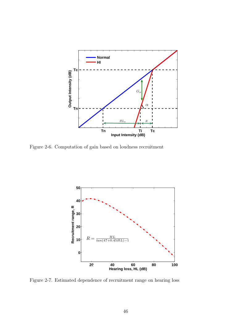
for the hearing-impaired the same as that for the normal-hearing. Figure 2-6 shows the

34

loudness relationship for the normal-hearing and the hearing-impaired. The blue line

shows the relationship between the sound levels judged to be at equal loudness by a

normal listener.

Tn represents the normal threshold of audibility and serves as a reference for the

typical impaired loudness growth which is shown in the red solid line. At the impaired

threshold, Ti, the perceived loudness is assumed to be equal to that of a signal at the

normal threshold Tn. At Tc, the threshold of complete recruitment, the loudness for the

impaired and the normal listener becomes the same.

In 1959, Hallpike and Hood [54] showed that the range of recruitment, Tc − Ti, is

a fairly orderly function of the hearing loss, Ti − Tn and is independent of frequency for

unilateral hearing loss. Miskolczy-Fodor [55] further reported this behavior for presbycusis.

Both these relationships are as shown in Figure 2-7.

Let α be defined as the angle between the recruitment curve and the horizontal axis

(Figure 2-6). The relation between α and hearing loss can be described by Equation 2–4.

α = 47 + 0.45HL (2–4)

Here hearing loss HL = Ti − Tn. If R = Tc − Ti is used to represent the recruitment

range, the relation between the recruitment range and hearing loss can be described by

Equation 2–5

R =HL

tanα− 1(2–5)

In order to achieve loudness normalization, the algorithm amplifies the signal in

each channel such that the output level is related to the input level by the solid line.

As the level is increased, the gain decreases until at Tc the gain becomes one. From

the audiogram, we can compute α and R and hence the gain factor per channel can

be computed. This approach which is based on the frequency independent relationship

between recruitment and hearing loss is called the recruitment based compensation (RBC)

method.

35

The gain for each channel GdB(w) is calculated as indicated by Equation set 2–6.

GdB(w) = Pout(w)− Pin(w)

Pout(w) = m(w)Pin(w) + b(w)

m(w) =R(w)

R(w) + HL(w)

b(w) = (1−m(w))Tc(w)

Tc(w) = R(w) + HL(w) + Tn(w)

R(w) =HL(w)

tanα(w)− 1

α = 47 + 0.45HL(w) (2–6)

Here HL(w) is the hearing loss at the center frequency of each band which is obtained

by the linear-interpolation of the audiogram. The RBC algorithm includes compression as

part of the prescription and the compression ratio for each channel is given by CR(w) =

1m(w)

. Compression is restricted to be within 1.1 and 3 for the hearing-impaired in order to

prevent any artifacts

While the existing algorithms which are also based on the concept of loudness

normalization require the loudness growth curve for each frequency or the average loudness

growth curves, all the RBC method requires is the audiogram of the hearing-impaired

person.

2.3 Parameter Analysis of RBC

2.3.1 Dynamic Constants of Compression

Compression is used to reduce the dynamic range of speech so that it can fit within

the reduced dynamic range of the hearing-impaired listener [56]. Compression can be

carried out either in a single band on in multiple bands. In multi-band processing, each

band usually has different compression characteristics and the degree of compression either

increases or decreases with frequency. Typically 2 or 3 bands are used. Increasing the

number of compression bands beyond 3 can result in audible distortion. Fitting algorithms

36

should always have output limiting compression to make sure that the sounds never get

painfully loud.

The attack and release times are the dynamic constants of compression and specify

how quickly a compressor operates. If the effect of compression is instantaneous audible

artifacts are produced because of the sudden change in levels. ANSI S3.22 defines the

attack time as the time taken for the output to stabilize within 3 dB of its final level after

the input changes from 55 to 90 dB SPL. The release time is defined as the time taken for

the output to stabilize within 4 dB of its final level after the input falls from 90 to 55 dB

SPL. Experimentally an attack time of 6 ms and a release time of 20 ms was found to be

ideal. The implementation of the attack and release time constants compression is given

by Equations 2–7.

Gave(w) = βattackGi(w) + (1− βattack)Gave(w)

Gave(w) = βreleaseGi(w) + (1− βrelease)Gave(w) (2–7)

Here Gave(w) is the average smoothed gain per band, Gi(w) is the instantaneous gain per

band, βattack and βrelease are the attack and release constants as defined in ANSI S3.22.

Compression ratio is the inverse of the slope of the input-output curve. The

compression ratio usually varies from 1.1:1 to 3:1. Compression threshold is the SPL

above which compression kicks in. If loudness is to be normalized completely, compression

should kick in from the threshold of normal-hearing which is 0 dB SPL [57]. But useful

speech sounds rarely occur below 30 dB SPL. When the compression threshold is > 50 dB

SPL it is termed as high-threshold and when the compression threshold is < 50 dB SPL it

is termed as low-threshold. Wide dynamic range compression (WDRC) refers to systems

which have low threshold. Figure 2-8 shows a typical WDRC characteristics with output

limiting.

Till the compression threshold of 50 dB, the gain is linear. Compression is effective

from after the threshold till the threshold of complete recruitment Tc(80 dB in this

37

example). The gain after Tc is linear till it reaches the output limiting compressor’s

threshold.

2.3.2 Filter Bank Analysis

The Matlab implementation of the RBC algorithm used 14 filter banks with center

frequencies equally spaced in Mel frequency between 100 Hz to fs/2. The number of filter

bank was chosen after listening experiments proved that 14 was the optimal number for

maximum cell phone speech intelligibility for the hearing-impaired (Figure 2-9).

In order to use RBC for the normal-hearing population a filter bank size of 5

was found to be optimal as a result of subjective listening tests. This is because

normal-hearing listeners can hear the artifacts caused because of multi-band gain. Also,

since typical normal-hearing population have little or no loudness recruitment effects, the

compression parameters varied from 1.1 to 1.5.

Compensation for reduced temporal and frequency resolution. The current

algorithm overcomes the decreased audibility and the loudness recruitment aspects of

sensorineural hearing loss by providing frequency and level dependent gain. By including

14 filter bands in 300–3400 Hz bandwidth we increase the frequency resolution. None of

the existing fitting algorithms include processing to overcome the reduced resolution in

time and frequency.

Dead regions of the cochlea. The RBC algorithm limits the amount of gain

per band based on the frequency and on the threshold of hearing for that band. If the

band has a loss ≥ 80 dB HL then the gain for that band is set to zero. This is done

because speech intelligibility decreases when the listening levels are loud. Also, high

frequency bands with high thresholds are penalized more than low frequency bands with

high threshold. Severe loss such as ≥ 80 dB HL usually occur due to damage to the

IHCs and OHCs. An area of non-functioning IHCs is referred to as a ‘dead region’. The

threshold equalizing noise (TEN) test [58] can be used clinically to detect dead regions

of the cochlea. It is similar to measuring thresholds of hearing in noise and measures the

38

threshold for detecting a tone in a threshold-equalizing noise. The dead frequency regions

are extrapolated to the filter band frequencies. Any band which lies in a dead region has

it’s gain set to zero. The first nearest neighbor frequency bands are also provided a gain

lower than usual.

2.3.3 Real-Time Implementation Issues

Audiogram on the phone. A Java midlet [59] was created to measure the

thresholds of hearing using the cell phone. Since the cell phone is to be used as an

assistive listening device for cell phone conversations and not a hearing aid, calibration is

not a key issue. The midlet plays tones at different levels and the listener presses a key

to indicate having heard the sound. The Motorola Roker E2 has 7 volume steps and by

playing scaled tone wave files a volume range from 3–65 dB was achieved. Figure 2-11

shows a depiction of how the audiogram on the phone would look.

2.4 Performance Analysis of the RBC Algorithm

The performance of RBC was compared with linear amplification (LA), a simple high

pass filter (HPF) [60], the DSL method, the HG method, the POGO method and the

NAL-R method. The speech database unless otherwise mentioned is the standard HINT

database. Cell phone speech was obtained by bandlimiting the speech to 300–3400 Hz

and then passing it through an AMBE vocoder/decoder block to introduced the vocoder

effects.

Experimental Setup. The HINT and the MOS listening tests were run at the

speech and hearing clinic, at the Gainesville Shands hospital in a sound treated booth

using the Sennheiser HDA 200 head phones. 10 hearing-impaired patients with a pure

tone average (500 Hz, 1 kHz, 2 kHz) of 40-70 dB HL were recruited. 10 normal-hearing

were also recruited. Figure 2-12 shows the audiograms of all the hearing impaired subjects.

Output limiting compression was provided for all the algorithms with a compression ratio

of 10:1 and a compression threshold of 110 dB.

39

2.4.1 Performance of Algorithm in Terms of Speech Quality

Both the subjective mean opinion score (MOS) test and the objective perceptual

evaluation of subjective quality (PESQ) scores were used to measure speech quality.

PESQ speech quality measurement for hearing-impaired and normal

hearing. To evaluate the performance of the new algorithm using PESQ the setup

shown in Figure 2-13 was used. Typical mild to severe sensorineural hearing loss and

typical normal-hearing were simulated using the Matlab hearing loss simulation block.

The audiograms used were: [10 20 30 60 80 90] dB HL and [5 10 15 20 20 20] dB HL

respectively. The unprocessed cell phone speech was passed through the hearing loss block

to generate simulated loss speech. Speech preprocessed by the various fitting algorithms

were passed through the hearing loss block to generate compensated speech.

The objective PESQ scores were obtained using the original cell phone speech as the

reference signal and comparing it to both the simulated loss speech and the compensated

speech (Figure 2-14).

PESQ is sensitive to distortion due to compression. The typical mild to severe SNHL

modeled here would provide output levels at high frequencies which would turn on the

output limiting compression. This results in low PESQ scores. If we compare with all

the compression based systems RBC does the best followed by DSL and NAL-R. The

scores also reveal that RBC outdid linear amplification and the other fitting algorithms for

normal-hearing subjects with an average PESQ score greater than “4-Good.”

Spectrograms for hearing-impaired and normal-hearing. The spectrograms for

the typical mild to severe SNHL simulated speech, linear-amplified speech and the speech

compensated using the RBC method were obtained (Figure 2-15). The simulated hearing

loss block was used to generate the speech (Figure 2-13).

For the hearing-impaired, a lot of high frequency information is missing (Figure 2-15a).

Linear amplification does not help because of the reduced dynamic range aspect of the

40

hearing loss (Figure 2-15b). Compression results in more high frequencies and this helps

improve intelligibility (Figure 2-15c).

The spectrograms for the typical normal-hearing simulated speech, linearly amplified

speech and the speech compensated using the RBC method were also obtained (Figure 2-16).

There is more high frequency information because of frequency dependent gain and this

helps improve intelligibility.

These results show that for both the normal-hearing and the hearing-impaired RBC

has better speech quality and more useful frequencies than with just a linear gain which is

what the cell phones volume control does.

Subjective speech quality measurement for hearing-impaired and normal

hearing: MOS. The MOS test provides subjective rating of speech quality in the absence

of noise. For the unaided hearing-impaired listeners speech was played at 75 dBA. For

normal-hearing listeners speech was played at 65 dBA. The Matlab MOS GUI was used to

run this test. Figure 2-17 shows the average of the MOS scores for the hearing-impaired.

For the hearing-impaired, RBC has an average MOS score greater than “4-Good.”

Figure 2-18 shows the average of the MOS scores for the normal-hearing. For the

normal-hearing, RBC has an average MOS score greater than “4-Good.”

2.4.2 Performance of Algorithm in terms of Speech Intelligibility

Both the subjective HINT test and the objective SII scores were used to measure

speech intelligibility.

Objective speech intelligibility measurement for normal-hearing: SII. The

speech intelligibility index (SII) was measured using the simulated hearing loss model for

normal-hearing. Cell phone bandwidth speech both unprocessed and processed by the

various fitting methods were passed through the simulated hearing loss block. The SII

standard does not give a valid score for hearing-impaired speech. Figure 3-7 shows the

variation of SII with SNR from -30 to 30.

41

For the normal-hearing, RBC does marginally better than linear amplification for

all SNR. An SII of 0.5 does not mean that speech is understandable 50% of the time. It

means that about 50% of the speech cues are audible. For conversational speech an SII of

0.5 corresponds to about 100% intelligibility for normal-hearing listeners.

Subjective speech intelligibility measurement for hearing-impaired and

normal hearing: HINT. The Matlab HINT GUI was used in this test. The 10

hearing-impaired and normal-hearing subjects listened to both unprocessed HINT

sentences and sentences processed by the different algorithms at various signal levels

in the presence of a constant 65 dBA noise. Figure 2-20 shows the averaged SNR for the

10 hearing-impaired subjects, with reference to the baseline (linear gain) for wide band

speech. These scores show that RBC does the best followed by DSL and half-gain. NAL-R

and half-Gain. When compared to the linear gain technique RBC provides upto 15 dB

improvement in SNR. The difference between RBC and DSL for wideband speech is about

3 dB.

Figure 2-21 shows the averaged HINT results with narrow band cell phone speech

input. These scores indicate that RBC does the best followed by NAL-R and half-gain.

Half-Gain prescribes a higher gain than all the fitting methods being tested. For loud

input levels, this will lead to a decrease in intelligibility but in the HINT the level of

speech is reduced so the gain increment helps half-gain do better. The difference between

RBC and linear gain is 15 dB. The difference between RBC and DSL for cell phone speech

is about 6 dB.

Figure 2-22 shows the averaged HINT results with narrow band cell phone speech

input. These scores show that RBC does the best followed by NAL-R and HPF. The

difference between RBC and linear gain is 6 dB. The difference between RBC and DSL for

cell phone speech is about 3 dB.

42

2.5 Summary

This chapter introduced a new hearing enhancement algorithm called recruitment

based compensation. RBC is based on loudness normalization and is used to fit the

cell phone to the user’s hearing thresholds. The RBC stage is followed by an output

limiting compressor to prevent damaging loud sound outputs. The performance of RBC

was measured in terms of objective and subjective measures of speech intelligibility and

quality. RBC was found to show consistent good performance.

Table 2-1: The kf constant for POGOFreq 250 500 1000 2000 4000kf -10 -5 0 0 0

Table 2-2: The kf constant for NALFreq 250 500 1000 2000 3000 4000kf -17 -8 1 -1 -2 -2

Figure 2-1. Classification of existing hearing aid fitting methods

43

Figure 2-2. Gains prescribed by the Fig6 method

Figure 2-3. Input-Output curve at 2 kHz obtained from the visual input output locator

44

Figure 2-4. DSL prescribed gain for different hearing loss

Figure 2-5. Recruitment based compensation system

45

Tn Ti Tc

Tn

Tc

Input Intensity (dB)

Ou

tpu

t In

ten

sity

(d

B)

NormalHI

α

Gw

RHLw

Figure 2-6. Computation of gain based on loudness recruitment

20 40 60 80 100

0

10

20

30

40

50

Hearing loss, HL (dB)

Rec

ruit

men

t ra

ng

e, R

R =HL

tan(47+0.45HL)−1

Figure 2-7. Estimated dependence of recruitment range on hearing loss

46

Figure 2-8. Compression input-output and gain curves

47

None RBC:2 RBC:3 RBC:4 RBC:5 RBC:7 RBC:9 RBC:12 RBC:14 RBC:20 RBC:32−30

−25

−20

−15

−10

−5

0

5

10

15

20

Algorithm:No of filter bands

Ave

SN

R w

rt b

asel

ine(

dB)

a

250 500 1000 2000 4000 80000

10

20

30

40

50

60

70

80

90

100

Frequency (Hz)

HL

(d

B)

Left ear

Right ear

b

Figure 2-9. Subjective HINT results for hearing-impaired A) Average HINT scores withvarying filter bank size B) Average audiogram of the hearing-impaired listeners

48

None HPF RBC:14NALR PG HG NALRP DSL

1−Bad

2−poor

3−Fair

4−Good

5−Excellent

Algorithm

a

250 500 1000 2000 4000 80000

10

20

30

40

50

60

70

80

90

100

Frequency (Hz)

HL

(d

B)

b

Figure 2-10. Subjective MOS results A) Average MOS scores for the hearing-impaired B)Audiogram of the hearing-impaired listeners

49

Figure 2-11. Audiogram on the phone Java midlet

Figure 2-12. Audiograms of all the hearing-impaired listeners

50

Figure 2-13. Hearing loss simulation system

Figure 2-14. The PESQ objective speech quality score for normal-hearing andhearing-impaired

51

ab

c

Fig

ure

2-15

.Spec

trog

ram

ofhea

ring-

impai

red

for

A)

Typic

alm

ild

tose

vere

SN

HL

B)

Lin

ear-

Am

plified

spee

chC

)R

BC

amplified

spee

ch

52

ab

c

Fig

ure

2-16

.Spec

trog

ram

ofnor

mal

-hea

ring

for

A)

Typic

alnor

mal

-hea

ring

B)

Lin

ear-

Am

plified

spee

chC

)R

BC

amplified

spee

ch

53


1−Bad

2−poor

3−Fair

4−Good

5−Excellent

Algorithm

a

250 500 1000 2000 4000 80000

10

20

30

40

50

60

70

80

90

100

Frequency (Hz)

HL

(d

B)

b


54


1−Bad

2−poor

3−Fair

4−Good

5−Excellent

Algorithm

a

250 500 1000 2000 4000 8000−10

−5

0

5

10

15

20

25

30

Frequency (Hz)

HL

(dB

)

b

Figure 2-18. Subjective MOS results A) Average MOS scores for the normal-hearing B)Audiogram of the normal-hearing listeners

55

Figure 2-19. Speech intelligibility index (SII) scores for normal-hearing as a function ofSNR

56

None HPF RBC NALR PG HG NALRPDSL−20

−15

−10

−5

0

5

Algorithm

Ave

. SN

R w

rt b

asel

ine

(dB

)

a

250 500 1000 2000 4000 800010

20

30

40

50

60

70

80

90

100

Frequency (Hz)

HL

(d

B)

b

Figure 2-20. Subjective HINT results with wide band speech for the hearing-impaired A)Average HINT scores B) Audiogram of the hearing-impaired listeners

57

None HPF RBC:14 NALR PG HG NALRP DSL−20

−15

−10

−5

0

5

Algorithm

Ave

. SN

R w

rt b

asel

ine(

dB)

a

250 500 1000 2000 4000 800010

20

30

40

50

60

70

80

90

100

Frequency (Hz)

HL

(d

B)

b

Figure 2-21. Subjective HINT results with cell phone speech for the hearing-impaired A)Average HINT scores B) Audiogram of the hearing-impaired listeners

58

None HPF RBC:14 NALR PG HG NALRP DSL−6

−5

−4

−3

−2

−1

0

1

2

Algorithm

Ave

. SN

R w

rt b

asel

ine(

dB)

a

250 500 1000 2000 4000 8000−5

0

5

10

15

Frequency (Hz)

HL

(dB

)

b

Figure 2-22. Subjective HINT results with cell phone speech for the normal-hearing A)Average HINT scores B) Audiogram of the normal-hearing listeners

59

CHAPTER 3NOISE ROBUST HEARING ENHANCEMENT ALGORITHMS

Environmental noise detrimentally affects the intelligibility of speech [61] and this

effect is more pronounced for people with hearing impairment. Speech is a highly

redundant signal. In a moderately noisy environment, a normal-hearing listener will

be able to understand what is being said even if some parts of the speech are masked

by noise by virtue of the redundant nature of speech. Hearing-Impaired listeners deal

with a less redundant speech signal because of the nature of their hearing loss [62]. This

implies that even if the environmental noise masks a smart portion of the remaining

speech, the intelligibility will be degraded significantly. The cochlea analyzes sound by

means of a group of highly overlapping narrow band filters. These filters are called the

critical bands and play an important role in noise masking. Only the noise which falls

within the same critical band as speech can mask the speech. But the same noise will

mask to a lesser extent, signals in higher frequency bands because of the highly overlapped

structure of the critical filter bank. This effect is called the upward spread of masking

and it increases with increase in noise intensity. This is also why low frequency sounds

are better speech maskers. For the hearing-impaired the critical bands will be more broad

and hence the upward spread of masking increases. This is why hearing-impaired listeners

require a 9 dB increase in SNR, when compared to normal-hearing listeners, in order

to understand speech in noise [25]. This chapter will discuss the development of a noise

robust recruitment based compensation (NR-RBC) algorithm.

3.1 Effects of Noise on Cell Phone Speech

Cell phone noise can be classified based on where it originates as the transmitter side

noise or the receiver side noise. The transmitter side environmental noise is often picked

up along with the speech and is transmitted as part of the outgoing signal. The channel

and vocoder produce some artifacts which are also transmitted. At the receiver end the

incoming signal is processed in order to remove or reduce the noise before it is played.

60

The receiver side environmental noise can mask the incoming cell phone speech. Table 3-1

provides a list of cell phone noise sources and suggests possible ways to reduce it.

3.2 Development of Noise Robust Recruitment Based Compensation

In order to reduce the effects of environmental noise masking at the listeners end,

the hearing enhancement algorithms have to be tuned to the noise. Hearing aid fitting

methods like DSL, NAL-R assume that a single frequency response is enough for speech

intelligibility under all listening conditions. But recent studies show that different

responses are desirable under different listening conditions. The factors that influence

the best setting are the noise spectrum and the noise level. In addition to the frequency

response, the best compression parameters also change with noise.

The RBC algorithm uses the audiogram in quiet information to prescribe the gains.

If masked thresholds of hearing are calculated then they can be used in the place of the

thresholds in quiet in the RBC estimation method. The algorithm will then vary the

gain and compression based on both the thresholds of hearing and the environmental

noise. This modified algorithm is called the noise robust recruitment based compensation

(NR-RBC) method.

Figure 3-1 shows the block diagram of the procedure. Here S(n) is the incoming

cell phone speech signal which is to be enhanced. Processing is carried out in the time

domain using a frame-by-frame approach. S(n) is fed to a filter bank which has 18 bands

with center frequencies and bandwidth as shown in Table 3-2. The environmental noise

is picked up by the cell phone’s calibrated microphone and is referred to as Y (n). The

microphone also picks up the user’s voice. In order to identify which frames contain noise,

Y (n) passes through a voice activity detection block. The noise frames are then fed to a

noise estimation block which provides an estimate of the noise for each octave-band. This

octave-band noise estimate is used to compute the noise masked thresholds. The gain

computation block uses the energy per band, the noise estimate and the user’s hearing

thresholds to prescribe a gain and compression term for each band as per the NR-RBC

61

formula. The signals from each band are finally combined together to get the enhanced

speech signal Se(c).

3.2.1 Single Microphone Noise Estimation

The cell phones microphone signal is referred to as Y (n) (Figure 3-1). During

pauses in the conversation Y (n) picks up the environmental noise. Using a voice activity

detection system the frames can be monitored for noise and speech. If a noise flag is set

then the noise power estimate is then updated. Using the single microphone system an

estimate of the environmental noise N(w) at the listeners end has to be calculated. This

will be done during pauses in the conversation. Techniques like Minima Controlled

Recursive Averaging (MCRA) [63] method and others [64] are available for robust

estimation of noise. We used a simple voice activity detector based on spectral distance.

3.2.2 Calculating the Noise Masking Threshold

The noise masking threshold is calculated for the incoming cell phone speech. If the

environmental noise lies below the noise masking threshold then the gain prescription

formula is the same as for RBC. The noise masking threshold can be obtained by modeling

the frequency selectivity and masking properties of the cochlea [65], [66]. As a first step

a critical band analysis has to be carried out in order to know which speech bands of

the incoming cell phone signal will be affected by the environmental noise. This can be

achieved by passing the noise through filter bank structure similar to the one used in

RBC 2-5. While this will lead to an accurate analysis, it will be computationally inefficient

to implement on the phone. A way to work around this is to group together the FFT bins

based on the critical band center frequencies and bandwidth. Table 3-2 lists the critical

band number, center frequency, bandwidth and the FFT bin details for a bin size of 256

and a sampling frequency of 8000 Hz.

Critical band analysis is carried out on the power spectrum of the signal over the

FFT bins which correspond to each critical band. 18 critical bands cover the cell phone

frequency range up to 4000 Hz. Since the critical bands are highly overlapped structures

62

the critical band power signal has to be convolved with a spreading function in order to

estimate the effects of masking across critical bands. The spreading function proposed by

Schroeder [67] is given by Equation 3–1

10 log10 Ti = 15.81 + 7.5(i + 0.474)− 17.5(1 + (i + 0.474)2)1/2 (3–1)

where, i is the critical band number and Ti is the spreading function.

The next step involves the calculation of the noise masking threshold, given by

Equation ??, which includes an offset term Oi which is specified in Table ??

Ti = 10log 10Ci−(Oi/10) (3–2)

The noise spread threshold has to be converted back to the Bark or critical band domain.

This is done by renormalization. The bark thresholds are compared to the individuals

absolute thresholds of hearing HL(w) also in the bark scale. The noise masking threshold

T (w) for any critical band which has a noise threshold lower than the absolute threshold is

changed to the absolute threshold.

3.2.3 Derivation of Noise Robust Recruitment Based Compensation

If the environmental noise is below noise masking thresholds for the speech, then the

usual RBC formula is used. If the noise is greater than the threshold of hearing then the

new gain can be calculated as follow:

The gain for each channel GdB(w) is calculated by Equation set 3–3.

HLn(w) = T (w) +(N(w)− T (w)

2, when T (w) < N(w) (3–3)

GdB(w) = Pout(w)− Pin(w)

Pout(w) = m(w)Pin(w) + b(w)

m(w) =R(w)

R(w) + HLn(w)b(w) = (1−m(w))Tc(w)

Tc(w) = R(w) + HLn(w) + Tn(w)

R(w) =HLn(w)

tanα(w)− 1

63

α = 47 + 0.45HLn(w)

3.3 Performance Analysis of the NR-RBC Algorithm

The performance of NR-RBC was compared with RBC and the other existing

algorithms in terms of subjective and objective measures of speech intelligibility and

quality.

Experimental setup. The HINT and the MOS listening tests were run at the

Shands speech and hearing clinic in a sound treated booth using a modified headset. The

modified device was shaped to look like a cell phone. 10 hearing-impaired patients with a

pure tone average (500 Hz, 1 kHz, 2 kHz) of 40–70 dB HL and 10 normal-hearing listeners

were recruited.

3.3.1 Performance of Algorithm in Terms of Speech Quality

Both the subjective mean opinion score (MOS) test and the objective perceptual

evaluation of subjective quality (PESQ) scores were used to measure speech quality.

PESQ speech quality measurement for hearing-impaired and normal

hearing. To evaluate the performance of the new algorithm using PESQ the setup

shown in Figure 2-13 was used. A typical mild to severe sensorineural hearing loss and

a typical normal-hearing was simulated using the Matlab hearing loss simulation block.

The audiograms used were: [10 20 30 60 80 90] dB HL and [5 10 15 20 20 20] dB HL.

The unprocessed cell phone speech was passed through the hearing loss block to generate

speech with simulated loss. Then speech preprocessed by the various fitting algorithms

were passed through the hearing loss block to generate compensated speech.

Among the HA fitting algorithms which include compression, NR-RBC has the

maximum PESQ score. For the normal-hearing NR-RBC had a slightly lower PESQ score

this could be due artifacts. In order to understand this the spectrograms of simulated

normal-hearing speech were calculated.

64

Spectrograms for hearing-impaired and normal hearing. Figure 3-3 shows

the spectrograms for the hearing-impaired speech, linearly amplified speech and the

speech compensated using the NR-RBC method. These results show that for the

hearing-impaired NR-RBC has better speech quality and intelligibility than with just

a linear gain which is what the cell phones volume control does. Figure 3-4 shows

the spectrograms for the normal-hearing speech, linearly amplified speech and the

speech compensated using the NR-RBC method. These results also show that for the

normal-hearing NR-RBC has better speech quality and intelligibility than with just a

linear gain.

Subjective speech quality measurement: MOS. The MOS test provides

subjective rating of speech quality in the absence of noise. For the unaided hearing-impaired

listeners speech was played at 75 dBA. For the normal hearing listeners speech was played

at 65 dBA. The room where the MOS test was conducted had a noise floor of in a room

with a noise floor of 46 dBA. The Matlab MOS GUI was used to run this test.

Figure 3-5 shows the average of the MOS scores for the hearing-impaired. For the

hearing-impaired, NR-RBC has an average MOS score greater than ‘4-Good’. Figure 3-6

shows the average of the MOS scores for the normal-hearing. For the normal-hearing,

NR-RBC has an average MOS score greater than ‘4-Good’.

3.3.2 Performance of Algorithm in terms of Speech Intelligibility

Both the subjective hearing in noise test (HINT) and the objective speech intelligibility

index (SII) scores were used to measure speech intelligibility.

Objective speech intelligibility measurement: SII. The SII was measured

using the simulated hearing loss model for normal-hearing. Cell phone bandwidth speech

both unprocessed and processed by the various fitting methods were passed through the

simulated hearing loss block. The sentences were then normalized and passed through

the SII measurement block while varying the SNR. It can be seen that NR-RBC has the

highest SII score at all SNRs.

65

Subjective speech intelligibility measurement: HINT. The Matlab HINT GUI

was used in this test. From the HINT tests in the Chapter 2 we know that RBC and DSL

show the best performance. The performance of NR-RBC was compared to RBC and DSL

with varying filter sizes.

Figure 3-8 shows the averaged SNR for the 10 hearing-impaired subjects, with

reference to the baseline (linear gain). It is clear that NR-RBC outperforms RBC and

DSL and has best performance at N=14 (Figure 3-8). The difference between NR-RBC

and the best DSL is about 20 dB.

Figure 3-9 shows the averaged SNR for the 10 normal-hearing subjects, with reference

to the baseline (linear gain). It is clear that NR-RBC outperforms RBC and DSL and

has best performance at N=8.The difference between NR-RBC and the best DSL is about

13 dB.

3.4 Summary

Environmental noise degrades the speech intelligibility for both normal-hearing and

hearing-impaired listeners though the degree of degradation is more for the hearing-impaired.

The recruitment based compensation algorithm was modified to include the noise term by

introducing the noise masked threshold. This leads to the noise robust recruitment based

compensation method (NR-RBC). This creates a fitting system which varies the gains

based on both the environment and the hearing thresholds. The noise robust recruitment

based compensation method was found to have good performance in terms of speech

intelligibility and quality for both the hearing-impaired and the normal hearing.

66

Table 3-1: Sources of cell phone noise and noise-reduction methodsCell phone noise Ways to reduce noiseReceiver side environment noise To prevent it from being transmitted:

Beamforming and AGCTo help you hear better: RBC algorithm(Automatically adjust gain)To help you hear better:Occlude contra-lateral ear

Transmitted environment noise To reduce its effects:Spectral subtraction

Vocoder and channel noise To reduce its effects:Spectral subtraction

Table 3-2: Critical bands and FFT binsCritical band details FFT details Noise masking

details N = 256, fs = 8kHz thresholdCritical band Center freq Bandwidth FFT critical band Offset term

number (Hz) (Hz) range (Hz) (dB)1 50 80 0 94 -172 150 100 94 187 -183 250 100 187 312 -194 350 100 312 406 -205 450 110 406 500 -216 570 120 500 625 -227 700 140 625 781 -238 840 150 781 906 -249 1000 160 906 1094 -2510 1170 190 1094 1281 -2511 1370 210 1281 1469 -2512 1600 240 1469 1719 -2513 1850 280 1719 2000 -2514 2150 320 2000 2312 -2515 2500 380 2312 2687 -2416 2900 450 2687 3125 -2317 3400 550 3125 3687 -2218 4000 700 3687 4000 -19

67

Fig

ure

3-1.

Noi

sero

bust

recr

uit

men

tbas

edco

mpen

sati

on(N

R-R

BC

)sy

stem

68

Fig

ure

3-2.

The

PE

SQ

obje

ctiv

esp

eech

qual

ity

scor

efo

rva

riou

sH

Afitt

ing

algo

rith

ms

69

ab

c

Fig

ure

3-3.

Spec

trog

ram

innoi

seof

hea

ring-

impai

red

for

A)

Typic

alm

ild

tose

vere

SN

HL

B)

Lin

ear-

Am

plified

spee

chC

)N

R-R

BC

amplified

spee

ch

70

ab

c

Fig

ure

3-4.

Spec

trog

ram

innoi

seof

nor

mal

-hea

ring

for

A)

Typic

alsi

mula

ted

nor

mal

-hea

ring

B)

Lin

ear-

Am

plified

spee

chC

)N

R-R

BC

amplified

spee

ch

71

None RBC:14 NR−RBC:14 DSL

1−Bad

2−poor

3−Fair

4−Good

5−Excellent

Algorithm

a

250 500 1000 2000 4000 80000

10

20

30

40

50

60

70

80

90

100

Frequency (Hz)

HL

(d

B)

b


72

None RBC:14 NR−RBC:14 DSL

1−Bad

2−poor

3−Fair

4−Good

5−Excellent

Algorithm

a

250 500 1000 2000 4000 8000−10

−5

0

5

10

15

20

25

30

Frequency (Hz)

HL

(dB

)

b

Figure 3-6. Subjective MOS results A) Average MOS scores for the normal-hearing B)Audiogram of the normal-hearing listeners

73

Figure 3-7. The SII scores for simulated normal-hearing as a function of SNR

Figure 3-8. The HINT scores for RBC (A1), NR-RBC (A2) and DSL (A3) with variationof filter size for hearing-impaired

74

Figure 3-9. The HINT scores for RBC (A1), NR-RBC (A2) and DSL (A3) with variationof filter size for normal-hearing

75

CHAPTER 4ACCLIMATIZATION MODELING FOR THE AIDED HEARING IMPAIRED

The auditory cortex undergoes physiological and anatomical changes over a period

of time when presented with altered auditory signal inputs. In the case of a person with

mild to severe SNHL, the altered auditory signal will have little or no high frequencies.

Moore [68] provided a review of studies showing evidence of plasticity in the auditory

system of the adult brain. Because of this brain plasticity, it takes time for the aided

hearing-impaired listeners to fully use the high-frequency information that they were

previously not used to hearing. This is known as the acclimatization effect. The time

period for acclimatization is defined as the period between when the hearing loss was

noticed and when the hearing aid was fitted.

Acclimatization is more pronounced for new hearing aid users and affects the hearing

aid fitting procedure. For a first time hearing aid user, the audiologist will first measure

the amount of loss, discuss the various hearing aid options (styles, binaural or monoaural)

and then choose a make and model of a hearing-aid. Ear mold measurements of the

patient are then made. The hearing aid will arrive after 2-3 weeks and the patient will be

‘fit’ with the hearing aid. Fitting is the procedure by which the hearing aid parameters

are tuned for the patient’s hearing loss. Usually, each hearing aid is accompanied by a

CD with the company’s proprietary fitting software which also allows selecting certain

established fitting procedures like DSL and NAL. As long as the initial fitting parameters

do not cause any discomfort, they will not be modified during the first visit. During the

follow up visits, the audiologist will fine-tune the parameters based on verbal feedback

from the patient. The verbal feedback is descriptive and indicates how certain sounds are

now being perceived with the hearing-aid. The patient is not asked to rate the sounds on

any scale. The fine-tuning process is repeated over multiple visits until the hearing aid

user is satisfied with a particular fitting. The follow up visits are usually apart by a couple

of weeks.

76

It is hypothesized that initially patients choose the amplification characteristics which

gives them the greatest gain at frequencies where they have the least loss because they

are used to hearing sounds at those frequencies. After a month, they then prefer high

frequency emphasis. It is also possible for patients to get acclimatized to a particular

hearing aid fitting. In such cases, the initial fitting parameters should be the optimum

ones. A compromise is to provide patients with a response that slowly varies over time

from the response they prefer to the response that is best for them. This will enable them

to gradually get used to a new response without subjecting them to a sound quality that

they are not happy with.

4.1 Development of the Fitting Satisfaction Scale

In the analysis of multi-session fitting data the final fitting parameters are considered

to be optimum since they provide the best sound experience for the patients. But this

definition of optimality is ambiguous since it can mean either best sound quality or best

speech intelligibility. This is because while manually adjusting the HA fitting parameters

audiologists rely on verbal patient feedback which is ambiguous. A better and more

structured approach would be to use a fitting satisfaction scale at each session to evaluate

the fitting.

The three main psychoacoustic phenomena associated with SNHL, elevated

threshold, loudness recruitment, and frequency blurring, lower the speech intelligibility

for hearing-impaired listeners by degrading the speech cues. Our previous research in

this area [69] has shown that SI based fitting methodologies show better performance in

noise and other real world scenarios. Hence it is better to use a rating scale, as shown

in Table 4-1, based on SI where 1 is low intelligibility and 5 is high intelligibility. It is

assumed that the listeners are not trained listeners, that the speech stimuli are sentences

and that the listeners have no prior cues about the speech stimuli.

77

4.2 Hearing Aid Fitting Data

4.2.1 Hearing Aid Fitting Data Collection

Multi-session fitting data was collected from patients using Phonak hearing aids (HA).

The Phonak HAs targeted were the Savia (30 patients), Claro (20 patients), Extra (7

patients), Valeo (4 patients), Perseo (3 patients) and Eleva (2 patients). All the patients

were fit binaurally. The left and right ear HAs were viewed as two separate inputs since

the audiograms for both the ears were different. The fitting software used with the

Claro used the desired sensation level (DSL) fitting procedure while the rest used the

national acoustic lab nonlinear (NAL-N1) procedure. Each HA users had 3-8 follow-up

sessions which were separated by a maximum of 3 months. The HA users used their

perception of speech to judge improvements between sessions and did not provide any

rating. Table 4-2 shows some of the fitting parameters provided by the listed Phonak HAs.

All HAs allow frequency based fine-tuning of the gain parameters and the maximum power

output (MPO) values at one or several input signal levels. Some hearing aids also allow

modification of the compression parameters (CR, TK, TK knee) across frequency.

4.2.2 Multi-Session Hearing Aid Fitting Data Analysis

Since most of the Phonal HAs use either NAL-NL1 or DSL[i/o], the fitting data of

one of each type was compared. National acoustic lab nonlinear (NAL-NL1) prescribes

gain which is similar to the NAL-R procedure but it also includes compression unlike

the NAL-R. NAL-NL1 prescribes less gain at the low frequencies compared to the other

suprathreshold methods and this is more evident at low input levels. DSL[i/o] and RBC

prescribe gain at lows in order to normalize loudness.

Figure 4-1 shows the variation of the 50 dB and 80 dB gains for the Claro HA, as

prescribed by DSL, between the first and last fitting. For the Claro, more people tend to

prefer having lesser gain at the final-fitting than at the initial-fitting. This goes against

our hypothesis that patients will slowly increase the HF gain. This could be explained by

78

the fact that DSL[i/o] has been known to over prescribe gain at 500Hz,2kHz and 4kHz at

both input levels [15].

Figure 4-2 shows the variation of the 40 dB and 80 dB gains for the Savia HA, as

prescribed by NAL-NL1, between the first and last fitting. For the Savia more people

prefer having higher gain at the final-fitting than at the initial-fitting. This could be

explained by the acclimatization process.

Figures 4-3 and 4-4 show the variation of the compression parameters for the Claro

and Savia HA. It can be seen that more people tend to not change TK for both Claro

and Savia. For Claro HAs, the change in compression ratio does not follow any conclusive

trend while for Savia the compression ratio seems to increase at the final fitting. This

could be explained by the fact that NAL-NL1 prescribes lesser CR at all frequencies

compared to the other suprathreshold methods [15].

In order to study the variation of the all the parameters for each HA, the trend in

change for each parameter was first averaged across the frequency. The maximum trend

across this average was then picked up and plotted for each HA in Figures 4-5 to 4-9.

For the Claro which was fit by DSL, from Figure 4-6it appears that the gain

parameters decrease at the final fitting while the TK, MPO parameters remain the

same and the CR decrease at the final fitting.

For the NAL-NL1 based HAs it appears that the frequency averaged gain parameters

increase at the final fitting. For Savia (Figure 4-5), Extra (Figure 4-7), and Valeo

(Figure 4-8) the frequency averaged compression parameters remain the same across

the fitting stages. For Eleva (Figure 4-9) and Perseo (Figure 4-10) the frequency averaged

compression parameters decrease across the fitting stages.

4.3 Modeling the Acclimatization Effect

A neural network (NN) can be used to model the variations from the initial fitting

to the final fitting (best response). The use of NNs in the area of hearing aids is not a

new thought. NNs have been used with HAs in the task of noise reduction [70] and to

79

help select the HA model based on the patient information [71]. J.M. Kates [72] studied

the feasibility of using NNs to derive HA prescriptive procedures. Kates concluded that

the factors which affected the accuracy of a NN based fitting method were the training

database size, the variability of the patient’s responses and the variability of the hearing

loss. Gao [73] proposed a new hearing prosthetics similar to the one proposed by Kates

which was based on NNs and fuzzy logic.

Rather than using NNs to replace existing fitting algorithms, we propose to use the

NNs along with the existing fitting algorithms to model the acclimatization effect. The

NN was trained on the multi-session fitting data using supervised learning. The input was

the initial fitting data and the desired was the final fitting data. In addition to the fitting

data, some HA user specific parameters such as patient’s age, degree of hearing loss (HL)

and the number of years with HL were used as inputs during training.

Figure 4-11 shows the structure of the NN used in the acclimatization modeling

setup. The NN used to model acclimatization was the multi-layer perceptron [74]. It had 7

sigmoidal input nodes and 7 linear output nodes. The number of hidden nodes was varied

until the lowest error was obtained and was found to be 4. Training was carried out using

the Levenberg-Marquardt [75] method with an initial global learning rate (LR) of 0.01.

Cross validation was used to stop the training in order to prevent over-training. The NN

was trained on the Savia data which had the most number of data points.

4.4 Performance Analysis of Model

The NN was trained using validation to prevent over-training. There were 60

multi-session data vectors for the Savia. The multi-session data was divided into 40

training sets, 10 validation sets and 10 test sets. 10 iterations with random initial weights,

training, testing and validation tests were run. A separate NN was used to model each

parameter The MSE error between the predicted and the target was used as our figure of

merit and comparison.

80

Figures 4-12to 4-17 show the results of training for the Savia HA. In the figures, the

red curve shows the MSE between the initial fitting values and the desired or optimal

values. From the figures, it can be observed that the gains predicted by the NN are

closer to the optimal values than by just using the initial values. There exists some error

between the predicted and the optimal values especially at the low frequencies and this

might be resolved by increasing the training database.

From the figures, it can be seen that the neural network succeeds in modeling the

trend with a certain amount of error. The error can be brought down by increasing the

training database. The MSE of the optimum setting is always less than that with the

initial setting.

4.5 Summary

Acclimatization occurs due to the plasticity of the auditory cortex. Fitting the HA

with the close to optimal solution at the first visit will both reduce the number of follow

up fitting sessions and result in a more optimum fit since the brain will get readjusted to

hearing the right frequencies from the first session. A neural network was trained to model

the variation of the change in parameters across fitting sessions for the Phonak Savia. The

results show a low test on new data MSE for all the parameters. A fitting satisfaction

scale based on SI was also proposed which will further help with the acclimatization

modeling by providing a statistic label to each session data.

Table 4-1: Speech intelligibility based fitting satisfaction scaleSpeech intelligibility ScoreSpeech is never intelligible 1

Speech is rarely intelligible 2

Speech is sometimes intelligible 3

Speech is usually intelligible 4

Speech is always intelligible 5

81

Tab

le4-

2:P

hon

akhea

ring

aid

fitt

ing

par

amet

ers

Hea

ring

Aid

sFit

ting

Input

Fre

quen

cy(k

Hz)

No

ofN

oof

par

amet

ers

leve

l(dB

)par

amet

ers

Pat

ients

Sav

iaG

ain

40

[0.3

0.88

1.7

2.4

3.5

7]

630

Gai

n60

[0.3

0.88

1.7

2.4

3.5

7]

630

Gai

n80

[0.3

0.88

1.7

2.4

3.5

7]

630

CR

-[0.3

0.88

1.7

2.4

3.5

7]

630

TK

-[0.3

0.88

1.7

2.4

3.5

7]

630

MP

O-

[0.3

0.88

1.7

2.4

3.5

7]

630

Cla

roG

ain

50

[0.25

0.5

0.75

1.2

23

5]

720

Gai

n80

[0.25

0.5

0.75

1.2

23

5]

720

CR

-[0.25

0.75

1.2

25]

520

TK

Knee

-[0.50

3]

220

TK

--

120

MP

O-

-1

20

Extr

aG

ain

40

[0.3

0.88

1.7

2.4

3.5

7]

67

Gai

n60

[0.3

0.88

1.7

2.4

3.5

7]

67

Gai

n80

[0.3

0.88

1.7

2.4

3.5

7]

67

CR

-[0.3

0.88

1.7

2.4

3.5

7]

67

TK

-[0.3

0.88

1.7

2.4

3.5

7]

67

MP

O-

[0.3

0.88

1.7

2.4

3.5

7]

67

Val

eoG

ain

50

[0.25

0.5

1.2

23

5]

64

MP

O-

-1

4

Per

seo

Gai

n50

[0.4

0.75

1.2

2.2

35]

63

Gai

n80

[0.4

0.75

1.2

2.2

35]

63

TK

-[

0.4

0.75

1.2

2.2

35]

63

MP

O-

[0.4

0.75

1.2

2.2

35]

63

82

a

b

Figure 4-1. Comparison of change from initial to final stage for Claro parameter A) 50 dBGain B) 80 dB Gain

83

a

b

Figure 4-2. Comparison of change from initial to final stage for Savia parameter A) 50 dBGain B) 80 dB Gain

84

a

b

Figure 4-3. Comparison of change from initial to final stage for Claro parameter A) TKand B) CR

85

a

b

Figure 4-4. Comparison of change from initial to final stage for Savia parameter A) TKand B) CR

86

L40:6 L60:6 L80:6 R40:6 R60:6 R80:6 RTk:6 LTk:6 RMpo:6 LMpo:6 RCr:6 LCr:60

2

4

6

8

10

12

14

16

18

20

Fitting Parameter:No of Frequencies

No

of

Pat

ien

ts

Final<InitFinal=InitFinal>Init

Figure 4-5. Phonak Savia maximum trend in fitting parameter variation averaged acrossfrequencies

L50:7 L80:7 R50:7 R80:7 RTk:2 LTk:2 RMpo:1 LMpo:1 RCr:5 LCr:5 RTKTh:1LTKTh:10

2

4

6

8

10

12

14

16


No

of

Pat

ien

ts


Figure 4-6. Phonak Claro maximum trend in fitting parameter variation averaged acrossfrequencies

87

L40:6 L60:6 L80:6 R40:6 R60:6 R80:6 RTk:6 LTk:6 RMpo:6LMpo:6 RCr:6 LCr:60

1

2

3

4

5

6


No

of

Pat

ien

ts


Figure 4-7. Phonak Extra maximum trend in fitting parameter variation averaged acrossfrequencies

88

L50:6 R50:6 RMpo:1 LMpo:10

0.5

1

1.5

2

2.5

3

3.5

4


No

of

Pat

ien

ts


Figure 4-8. Phonak Valeo maximum trend in fitting parameter variation averaged acrossfrequencies

89

L40:6 L60:6 L80:6 R40:6 R60:6 R80:6 RTk:6 LTk:6 RMpo:6 LMpo:6 RCr:6 LCr:60

0.2

0.4

0.6

0.8

1

1.2

1.4

1.6

1.8

2


No

of

Pat

ien

ts


Figure 4-9. Phonak Eleva maximum trend in fitting parameter variation averaged acrossfrequencies

90

L50:6 L80:6 R50:6 R80:6 RTk:6 LTk:6 RMpo:1 LMpo:10

0.5

1

1.5

2

2.5

3


No

of

Pat

ien

ts


Figure 4-10. Phonak Perseo maximum trend in fitting parameter variation averaged acrossfrequencies

91

Figure 4-11. Structure of the MLP used to model multi-session fitting trends

92

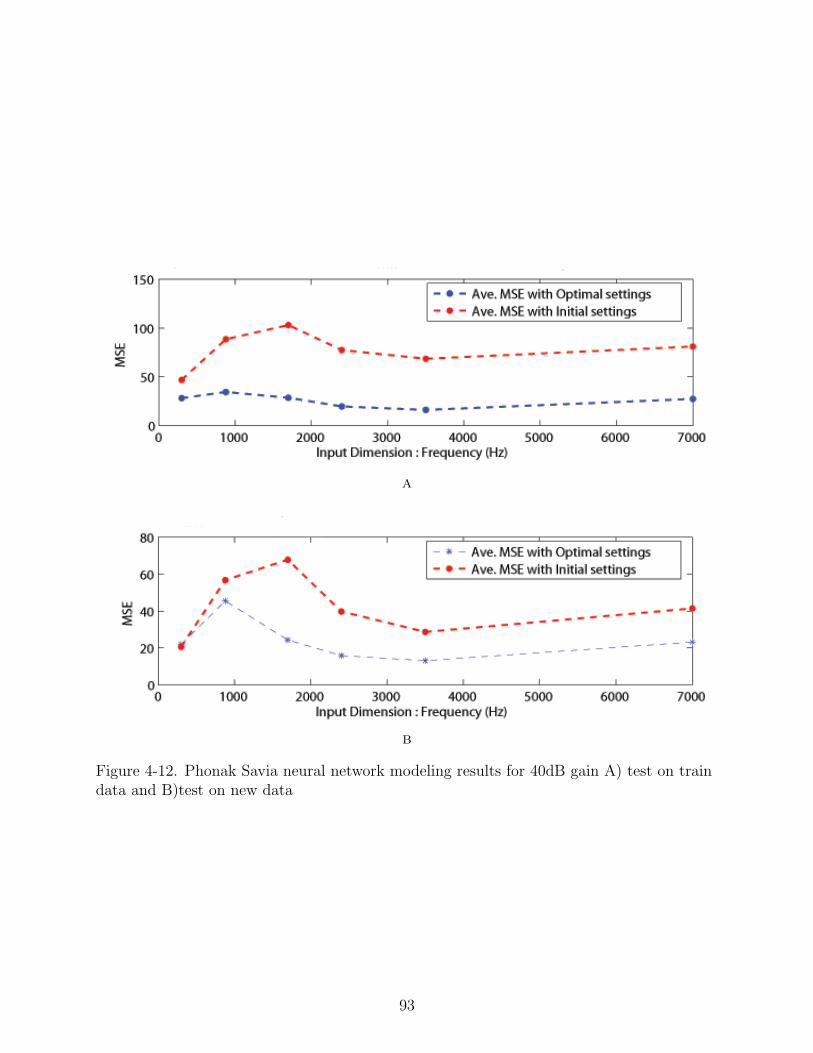
a

b

Figure 4-12. Phonak Savia neural network modeling results for 40dB gain A) test on traindata and B)test on new data

93

a

b


94

a

b


95

a

b

Figure 4-15. Phonak Savia neural network modeling results for CR parameter A) test ontrain data and B)test on new data

96

a

b

Figure 4-16. Phonak Savia neural network modeling results for TK parameter A) test ontrain data and B)test on new data

97

a

b

Figure 4-17. Phonak Savia neural network modeling results for MPO parameter A) test ontrain data and B)test on new data

98

CHAPTER 5CONCLUSIONS

The US census bureau states that 50 million people, nearly one-fifth of the US

population, are in some way disabled. Among this 28 million people are hearing-impaired.

With suitable technological assistance these men and women (notably the aging baby

boomers) may prolong their independence and reduce their need for specialized care.

Their quality of life will be improved. While no product can be designed so that every

single person in the world can use it, the intent is to maximize the potential of each

device. This dissertation proposes using the cell phone as an assistive listening device.

This will enable the 20 million hearing-impaired people who do not use hearing aids

understand cell phone speech better. This will also help normal-hearing listeners especially

in noise situations.

Sensorineural hearing loss (SNHL) is mostly caused by damage to the outer hair

cells (OHC). So in particular, the hearing loss compensation algorithm has to replace

the damaged outer hair cells. A novel algorithm based on the frequency independent

relationship between hearing loss and recruitment was developed. This recruitment based

compensation (RBC) algorithm prescribes both the gains and compression parameters.

RBC shows a 15 dB improvement in speech intelligibility when compared to the baseline

algorithm (linear gain) for the hearing-impaired. For the normal hearing the SNR

difference between RBC and linear gain is 6 dB. By providing frequency dependent

gain and compression the decreased audibility and decreased dynamic range aspects of

SNHL are overcome. This is carried out by processing the speech signal in 14 filter banks.

The filter banks have their centers equally spaced in mel frequency and is so designed

keeping the auditory processing of the OHCs in mind.

The OHCs lose their abilities to increase the sensitivity of the cochlea for frequencies

to which the affected part of the cochlea is tuned. Psychoacoustically, this shows

up as flatter tuning curves. Because of this, noise has a greater masking effect for

99

hearing-impaired people. The noise robust recruitment based compensation (NR-RBC)

algorithm was developed to improve the performance of RBC in noise. NR-RBC uses a

noise estimate to calculate the noise masked threshold for speech which is used in the

gain prescription. NR-RBC outperforms RBC and DSL in terms of speech intelligibility.

The difference between NR-RBC and DSL for the hearing-impaired is 20 dB and for the

normal-hearing is 13 dB. Both RBC and NR-RBC have a MOS speech quality rating of

‘Good’.

The auditory cortex undergoes physiological and anatomical changes in the

presence of altered auditory input. Because of this brain plasticity, it takes some time

for the hearing-impaired to learn to fully use the high-frequency information that

they were previously not used to hearing. This is known as the acclimatization effect.

Multiple-session data for a number of Phonak hearing aids was collected and analyzed.

Neural network were used to model the acclimatization effect in hearing aid fitting. Low

mean square error (MSE) for test on new data was obtained.

Contribution summary. Three novel hearing enhancement algorithms were

developed as part of this multi-disciplinary research which was the result of a proposal

written by us. A cell phone hearing evaluation questionnaire was created to understand

the needs of the hearing-impaired. Focus group meetings were conducted and video

testimonials were obtained to further narrow down on the main problems faced by the

hearing-impaired. Higher speech intelligibility was found to be a main requirement.

Three novel algorithms all based on the rationale of maximizing speech intelligibility

were created. RBC is aimed towards helping both normal-hearing and unaided hearing-impaired

listeners understand cell phone speech better. NR-RBC is a noise robust technique which

enhances the hearing in noise. Acclimatization modeling is proposed to improve the

quality of the initial fit for the aided hearing-impaired listener. The hearing enhancement

algorithms were tested extensively in terms of objective and subjective measures of speech

quality (SQ) and intelligibility (SI) on both normal-hearing and hearing-impaired subjects

100

and were shown to have good performance in terms of both quality and intelligibility. A

FFT based filter bank approach to implement both RBC and NR-RBC was also proposed

which leads to an easy realtime implementation. Matlab code was written for the hearing

loss simulation, for the audiogram GUI, for the three new algorithms, for all the popular

hearing aid fitting methods mentioned in this dissertation, for the automated subjective SI

and SQ tests.

101

APPENDIX ASURVEY OF HEARING-IMPAIRED CELL PHONE USERS

This chapter discusses the results of the cell phone hearing evaluation survey. 84

hearing-impaired participants answered 20 hearing aid and cell phone related questions

and provided other relevant demographic information. The questionnaire used in the

survey is available in Appendix B.

A.1 Participants

84 subjects with hearing loss were recruited from four different University of Florida

clinics during patient visits and voluntarily completed the surveys in the fall of 2004

and spring of 2005.. All participants were previous or current cell phone users. The

participants’ hearing impairment ranged from mild to profound and the distribution is

shown in Figure A-1. Hearing aid usage experience varied among the subjects. Subjects

ranged from 23 to 89 years of age with a mean age of 66.32 years old. Fifty-two males and

32 females participated in the survey.

A.2 Results

Review of the completed surveys showed some questions were left unanswered by

some participants. Therefore, the survey data posted below indicates the number of

participants who responded to each question.

A.2.1 Cell Phone Usage

Of the 84 participants, 62 were experienced hearing aid users and the remaining 22

had not tried hearing aids. Five of the 62 hearing aid users were fit unilaterally and the

other 57 were fit binaurally. Only 4 of the 62 hearing aid users wore completely in canals

(CICs) and the remaining hearing aid styles were almost evenly split between behind the

ears (BTEs) and in the ears (ITEs). Sixty-one cell phone users indicated their estimated

time spent on their cell phone and the results showed that 8 individuals use their cell

phone just for emergencies, 7 reported over 400 minutes of use each month, while the

remaining 45 reported less than 400 minutes on the cell phone each month. The average

102

age of respondents who reported frequent cell phone usage was 61.6 years while those who

used their phones less frequently was 70.0 years, and finally those who reported they do

not use their cell phone frequently was 75.6 years. Sixty respondents identified the style

of cell phone they use, and 55% indicated that their cell phone was a flip phone while the

other 45% used a candy bar style phone. Two cell phone users used neckloops.

A.2.2 Electromagnetic Interference

14 of 35 hearing aid users indicated that their cell phone created EM interference

in their hearing aid and 8 of these 14 reported that the noise was so severe that it had

prevented them from using their cell phone. Two participants thought that the noise

might have occurred and were not sure about it, while two others experienced interference

from the cell phone backlight. Analysis of variance indicated that 78% of respondents who

reported noise in their hearing aid used candy bar style cell phones and the other 22%

were flip phone users. The two individuals who used neckloops expressed concern that the

neckloop would not be compatible with other phones. Other individuals commented that

they were not interested in buying any additional equipment to make their hearing aids

compatible with their cell phone.

A.2.3 Cell Phone Speech and Ringer Level

One in three of the hearing-impaired cell phone users reported trouble hearing their

cell phone ring. 31.8% of cell phone users who did not use hearing aids had trouble

hearing the ringer. 31 of 54 cell phone users desired louder cell phone speech levels and

1/3rd of those desiring more volume were non-hearing aid users. The need for higher cell

phone output level was also shared by persons with hearing loss ranging from mild to

profound. Figure A-2 indicates the self-reported understanding of cell phone speech in

quiet and in noise for both aided and unaided hearing-impaired participants.

A.2.4 Summary and Conclusions

The results of the survey indicate that a large percentage of the hearing-impaired

have difficulty using the cell phone effectively because of obstacles such as electromagnetic

103

(EM) interference and insufficient cell phone signal and ringer volume. ANSI standard

C63.19 [6] indicates how hearing aid and cell phone manufacturers should measure the

EM interference. The measurements are translated into M-ratings in which the higher

ratings indicate a lower likelihood of interference. Handsets that receive a hearing aid

compatibility rating of M3 or higher have met or surpassed FCC requirement. The FCC

has required that cell phone companies have 50% of their handsets meet a minimum ANSI

rating of M3 or better by February 18, 2008.

Figure A-1. Degree of hearing impairment among survey participants

104

Figure A-2. Degree of hearing impairment for survey participants

105

APPENDIX BCELL PHONE HEARING EVALUATION QUESTIONNAIRE

1. Is your hearing loss:

(a) Mild- A little difficulty hearing speech

(b) Moderate- More difficulty hearing speech

(c) Severe- A lot of difficulty hearing speech

(d) Profound- So bad that hearing aids may not help

2. Do you use Hearing aids?

(a) Yes

(b) No

3. Your Left Ear Hearing aid is:

(a) None

(b) ITE- In The Ear

(c) BTE-Behind the Ear

(d) CIC-Completely In Canal

(e) Other

4. Your Right Ear Hearing aid is:

(a) None

(b) ITE- In The Ear

(c) BTE-Behind the Ear

(d) CIC-Completely In Canal

(e) Other

5. What is the make and model of your Hearing aid?

6. Check whichever is true:

(a) I can understand speech over the telephone with my hearing aid

106

(b) I can understand speech over the telephone in noisy environments with my

hearing aid

(c) I can understand speech over the telephone without my hearing aid

7. Does your Hearing aid have a telecoil?

(A feature available on many hearing aids is the telecoil or t-switch or t-coil which

aids in hearing telephone conversations.)

(a) Yes

(b) No

8. If your Hearing aid has a telecoil, do you use your telecoil with your cell phone?

(a) Yes

(b) No

(c) I don’t use cell phones

9. Do you frequently use cell phones?

(a) Yes

(b) No

10. Check whichever is true: What has been your general experience with cell phones?

(a) I can understand speech on the cell phone

(b) I can understand speech on the cell phones in noisy environments

(c) I have trouble hearing my cell phone ring

(d) I cannot understand speech on the cell phones because:

If you don’t use cell phones regularly jump to question 17 else continue

11. What is the make and model of the cell phone you use?

(Example Make= Motorola Model=v300)

12. Is it a Flip phone?

(a) Yes

107

(b) No

13. Do you use a neckloop for cell phone conversations?

(A neckloop is a necklace-size loop of wire worn around the neck of someone who has

a hearing aid with a telecoil.)

(a) Yes

(b) No

14. Which Cell phone Network provider do you use?

(a) Cingular

(b) Tmobile

(c) Verizon

(d) Sprint

(e) Other

15. How many minutes per month do you talk on the cell phone?

(a) Just for emergencies

(b) <200

(c) 200-400

(d) 400+

(e) Don’t know

16. Check whichever is true:

(a) I wish my cell phone would be louder

(b) My cell phone create noise in my Hearing aid

(c) This noise prevents me from using my cell phone

(d) A person talking near me on a cell phone produces noise in my Hearing aid

17. Does your cell phone backlight cause noise in your Hearing aid?

(a) Yes

(b) No

(c) Not noticed

108

18. Would you be interested in a combination Hearing aid and cell phone?

(a) Yes

(b) No

19. Is there enough information available online to help you choose the cell phone right

for you?

(a) Yes

(b) No

20. What information regarding cell phones and hearing aids would you like to see

available?

109

APPENDIX CANALYSIS OF THE FOCUS GROUP DISCUSSIONS

In order to better understand the needs of the hearing-impaired population two

focus groups with hearing-impaired participants were conducted. This chapter provides a

synopsis of the main themes which were observed at the two focus group.

C.1 Participants

The two focus groups were held on 06/18/2004 and 09/24/2004 at the University

of Florida speech and hearing clinic at Shands hospital in Gainesville. Focus group one

lasted approximately two hours and was attended by 3 hearing-impaired subjects. All of

them were hearing-aids users and and had used cell phones. Focus group two was attended

by 10 hearing-impaired subjects. All of them owned hearing aids and had used cell

phones.The hearing-impaired participants were informed that they were at the meeting to

give their opinions, answer questions, ask questions, nominate topics and generate ideas.

The sessions were audio taped and later transcribed.

C.2 Focus Group Main Themes

C.2.1 Aided Cell Phone Listening Problems

The placement of the microphones in the behind the ear (BTE) hearing aids makes

it tricky to couple the cell phone loudspeaker output to the hearing aid. There was the

worry that, in trying to find the ‘sweet spot’ for the BTE hearing aid (HA), the phone

would be placed at such an odd angle that the person on the other end would not be able

to hear you speak. Some people find it easier to remove their HAs to use the cell phone

but do not like doing so. The HA volume had to be at maximum to hear the cell phone

conversation and this caused feedback for the in the ear (ITE) hearing aids. Louder cell

phone output was requested by all. Some participants reported electromagnetic (EM)

interference between the cell phone and the HA. There was also trouble hearing the phone

ring.

110

C.2.2 Ideal Hearing Aid Compatible Cell Phone

The ideal cell phone would be one which would not have any feedback or placement

problems. It would have volume control which would allow for louder levels and which

would offer frequency based adjustments so as to match their unique losses. The phone

would be a flip-phone style which was found to have less EM interference with the HA.

It would have a hands-free option where it could be directly coupled to the hearing-aid.

Control over the ring tone volume level and frequency would also be provided.

C.2.3 Comments on a Cell Phone Assistive Listening Device

There was the thought that one could wear one normal hearing aid on one ear and a

handsfree cell phone assistive listening device (ALD) on the other ear.The idea of taking

a hearing test on the cell phone was favored by all. There was some worry about whether

the phone would be too loud and the option of fitting the phone at the audiology clinic

was mentioned. There was the thought that fitting a cell phone to meet a hearing loss and

also using the HA might provide the increase in volume required to hear speech especially

for those with high losses. A hands-free solution, similar to a bluetooth headset, was

appreciated. In the absence of a hands free solution, there was worry over taking out the

HA in order to use the phone.

111

APPENDIX DPHYSIOLOGY OF HEARING

The human ear, the organ of hearing and balance, is the best example of an

engineering masterpiece. It enables us to hear sounds ranging from 20 Hz-20 kHz with

a dynamic range of 0-130 dB. Anatomically, the human ear can be divided into three

parts: the outer ear (pinna, auditory canal), the middle ear (ossicles, eardrum, oval

window) and the inner ear (cochlea, semicircular canals). Figure D-1, shows the internal

structure of the ear.

The human pinna is symmetric, points forward and has a curved structure. It focuses

sound pressure waves into the auditory canal. The structure of the pinna aids in sound

localization. Horizontal localization is made possible because of inter-aural time and

intensity differences while vertical localization is made possible because of the frequency

shaping of the sound by the curves of the pinna. The auditory canal which is around

2.7 cm in length acts as a 14

wave closed tube resonator and boosts the 2-5 kHz region by

15 dB. The broad resonance peak is because the closed end of the auditory canal is the

pliant ear drum or tympanic membrane.

The middle ear consists of the eardrum, the ossicles (malleus, incus and stapes) and

the oval window. The ossicles translate the sound pressure wave to vibrations in the

cochlea. They provide impedance matching since the acoustic impedance of the fluid

in the cochlea is about 4000 times that of air. The ossicles provide amplification by

lever action (3x) and by terms of area amplification (15x). The ossicles also help block

very loud low frequency sounds by means of the stapedius reflex. The stapes transmits

vibrations to the oval window on the outside of the cochlea. This moves the fluid in the

cochlea which forms a traveling wave, with a peak at one location along the length of the

cochlea. Conductive hearing loss occurs when sound is not conducted efficiently to the

cochlea through the ossicles. The cochlea is intact for conductive hearing loss.

112

The cochlea is the body’s microphone. It converts the mechanical movement into

electrical action potentials which are then carried to the brain through the auditory nerve.

The cochlea is a snail-shell like structure and contains three fluid filled canals. One of

them the organ of corti has a lining called the basilar membrane (BM). Hair cells are

arranged in four rows along the entire length of the cochlear coil (Figure D-2). Three rows

consist of outer hair cells (OHCs) and one row consists of inner hair cells (IHCs). Each

hair cell has hundreds of tiny stereocilia. The stereocilia of the OHCs are embedded in

the tectorial membrane. The traveling wave bends the IHC’s stereocilia and this produces

action potentials.

The afferent IHCs transmit signals to the brain via the auditory nerve. The efferent

OHCs receive neural input from the brain which influences its motility as part of the

cochlea’s mechanical pre-amplifier. The OHCs help the IHCs sense soft sounds by

sharpening the peak of the traveling wave. Based on feedback from the brain, the OHCs

mechanically shrink pulling down the tectorial membrane. Once the IHCs cilia brushes

against the tectorial membrane, action potentials are generated. In addition to amplifying

soft sounds, OHCs also sharpen the peak of the traveling wave resulting in high frequency

resolution. Sensorineural hearing loss occurs because of damage to the hair cells. Hearing

loss due to aging or presbycusis is a type of sensorineural hearing loss and occurs due to

wear and tear of the hair cells. A hearing loss up to 60 dB HL can be considered to be

because of OHCs and anything higher than 80 dB HL is because of both IHC and OHC

damage. Figure D-3, shows the hair cells for a person with normal-hearing and a person

with severe hearing loss. Damage to the OHCs indicates a lower frequency resolution

and the inability to hear soft sounds while damage to the IHCs indicates that the sound

information is not being sent to the brain.

There is a tonotopic mapping along the length of the BM (Figure D-4). Each part of

the BM has a characteristic frequency of maximum vibration which depends on its relative

position. At the base of the cochlea (near the oval window), the BM is stiff and thin and

113

hence more responsive to high frequencies. The apex of the cochlea is wide and floppy and

more responsive to low frequencies. Each IHC has about 10 auditory nerve (AN) fibers.

The AN fibers also have a tonotopic mapping and encode steady state sounds and onsets.

At the stimulus onset, the AN firing increases rapidly. For constant stimulus, the firing

rate decreases exponentially. The AN pathway passes from the cochlea to the brainstem

and then upwards to the auditory processing centers of the temporal lobes of the brain

which decode the neural signal and provides us with the sensation of sound.

Figure D-1. Structure of the human ear [76]

114

Figure D-2. Hair cells of the Organ of corti [77]

a b

Figure D-3. Electron micrograph of the organ of corti for A) Normal-hearing B) Severehearing loss [78]

115

Figure D-4. Frequency sensitivity of the basilar membrane

116

REFERENCES

[1] S. Arlinger, “Negative consequences of uncorrected hearing loss–a review,” Interna-tional Journal of Audiology, vol. 42, pp. S17–20, 2003.

[2] “CTIA semi-annual wireless industry survey,” (updated 2007; cited December 2007).[Online]. Available: http://files.ctia.org/pdf/CTIA Survey Mid Year 2007.pdf, CTIA,Washington, DC.

[3] Statistics about hearing disorders, ear infections, and deafness. (updated January2007; cited December 2007). [Online]. Available: http://www.nidcd.nih.gov/health/statistics/hearing.asp. NIDCD. Bethesda, MD.

[4] M. C. Killion, “The SIN report: Circuits haven’t solved the hearing-in-noiseproblem,” The Hearing Journal, vol. 50, p. 10, 1997.

[5] M. Skopec, “Hearing aid electromagnetic interference from digital wirelesstelephones,” IEEE Transactions On Rehabilitation Engineering, vol. 6, pp. 235–239,1998.

[6] American National Standard for Methods of Measurement of Compatibility betweenWireless Communications Devices and Hearing Aids, ANSI Std. C63.19-2005, 2005.

[7] J. Rodman, “The effect of bandwidth on speech intelligibility,” White Paper,Polycom, 2003.

[8] B. C. J. Moore, “Perceptual consequences of cochlear hearing loss and theirimplications for the design of hearing aids,” Ear and Hearing, vol. 17, pp. 133–161,1996.

[9] T. Venema, Compression for Clinicians. San Diego, CA: Singular Publishing Group,1999.

[10] Noise induced hearing loss facts. (updated 2007; cited December 2007). [Online].Available: http://www.hei.org/news/facts/nihlfact.htm. HEI. Los Angeles, CA.

[11] C. Portnuff. Safe listening levels for apple iPod. (updated October 2006; citedDecember 2007). [Online]. Available: http://www.physorg.com/news80304823.html.Boulder, CO.

[12] Occupational Safety and Health Standards, Occupational Safety and HealthAdministration Std. 1910.95, 1983.

[13] Criteria for a Recommended Standard: Occupational Noise Exposure Publication,National Institute for Occupational Safety and Health Std. 98-126, 1998.

[14] J. W. Hall and H. G. Mueller, Audiologists’ Desk Reference Volume I: DiagnosticAudiology Principles Procedures and Protocols. San Diego, CA: Singular PublishingGroup, 1996.

117

http://files.ctia.org/pdf/CTIA_Survey_Mid_Year_2007.pdf

http://www.nidcd.nih.gov/health/statistics/hearing.asp

http://www.nidcd.nih.gov/health/statistics/hearing.asp

http://www.hei.org/news/facts/nihlfact.htm

http://www.physorg.com/news80304823.html

[15] H. Dillon, Hearing Aids. New York: Thieme Medical Publishers; 1st edition, 2001.

[16] M. C. Killion, “SNR loss: I can hear what people say, but i can’t understand them,”The Hearing Review, vol. 4, pp. 8–14, 1997.

[17] J. H. Macrae and H. Dillon, “Gain, frequency response, and maximum outputrequirements for hearing aids,” Journal of Rehabilitation Research and Development,vol. 33, no. 4, pp. 363–76, 1996.

[18] J. C. Steinberg and M. B. Gardner, “The dependence of hearing impairment on soundintensity,” Journal of the Acoustical Society of America, vol. 9, no. 1, pp. 11–23, 1937.

[19] B. A. Henry, C. W. Turner, and A. Behrens, “Spectral peak resolution and speechrecognition in quiet: Normal hearing, hearing impaired, and cochlear implantlisteners,” Journal of the Acoustical Society of America, vol. 118, pp. 1111–1121,2005.

[20] B. R. Glasberg and B. C. J. Moore, “Psychoacoustic abilities of subjects withunilateral and bilateral cochlear hearing impairments and their relationship to theability to understand speech,” Scandinavian Audiology, vol. 32, pp. 1–25, 1989.

[21] E. Zwicker and K. Schorn, “Psychoacoustical tuning curves in audiology,” Audiology,vol. 17, pp. 120–40, 1978.

[22] E. M. Danaher and J. M. Pickett, “Some masking effects produced by low-frequencyvowel formants in persons with sensorineural hearing loss,” Journal of Speech andHearing Research, vol. 18, pp. 261–71, 1975.

[23] J. R. Dubno and A. B. Schaefer, “Frequency selectivity for hearing-impaired andbroadband-noise-masked normal listeners,” Quarterly Journal of ExperimentalPsychology, vol. 43, pp. 543–64, 1991.

[24] E. M. Danaher, M. P. Wilson, and J. M. Pickett, “Backward and forward masking inlisteners with severe sensorineural hearing loss,” Audiology, vol. 17, pp. 324–38, 1978.

[25] S. Hygge, J. Ronnberg, and B. Larsby, “Normal-hearing and hearing-impairedsubjects’ ability to just follow conversation in competing speech, reversed speech, andnoise backgrounds,” Journal of Speech and Hearing Research, vol. 35, pp. 208–15,1992.

[26] B. C. J. Moore and B. R. Glasberg, “Simulation of the effects of loudness recruitmentand threshold elevation on the intelligibility of speech in quiet and in a backgroundof speech,” Journal of the Acoustical Society of America, vol. 94, pp. 2050–2062, Oct.1993.

[27] Y. Nejime and B. C. J. Moore, “Simulation of the effect of threshold elevation andloudness recruitment combined with reduced frequency selectivity on the intelligibilityof speech in noise,” Journal of the Acoustical Society of America, vol. 102, no. 1, pp.603–615, 1997.

118

[28] P. Duchnowski and P. M. Zurek, “Villchur revisited: Another look at automatic gaincontrol simulation of recruiting hearing loss,” Journal of the Acoustical Society ofAmerica, vol. 98, no. 6, pp. 3170–3181, 1995.

[29] P. W. Barnett, “Overview of speech intelligibility,” in Proceedings of the Institute ofAcoustics, vol. 21, 1999.

[30] K. Kasturi, P. Loizou, M. Dorman, and T. Spahr, “The intelligibility of speech withholes in the spectrum,” Journal of the Acoustical Society of America, vol. 112, 2002.

[31] N. R. French and J. C. Steinberg, “Factors governing the intelligibility of speechsounds,” Journal of the Acoustical Society of America, vol. 19, p. 90, 1947.

[32] J. D. Miller, “Effects of noise on people,” Journal of the Acoustical Society of Amer-ica, vol. 56, pp. 724–764, 1974.

[33] S. Fidell, R. Horonjeff, and S. Teffeteller, “Effective masking bandwidths at lowfrequencies,” Journal of the Acoustical Society of America, vol. 73, pp. 628–38, 1983.

[34] G. Parikh and P. Loizou, “The influence of noise on vowel and consonant cues,”Journal of the Acoustical Society of America, vol. 118, pp. 3874–3888, 2005.

[35] L. M. Jenstad and P. E. Souza, “Quantifying the effect of compression hearing aidrelease time on speech acoustics and intelligibility,” Journal of Speech, Language andHearing Research, vol. 48, pp. 651–67, 2005.

[36] R. V. Shannon, F. Zeng, and V. Kamath, “Speech recognition with primarilytemporal cues,” Science, vol. 270, pp. 303–304, 1995.

[37] Hearing in noise test. (updated June 2005; cited December 2007). [Online]. Available:http://www.californiaearinstitute.com/audiology/hint.php. California Ear Institute.Palo Alto, CA.

[38] American National Standard Methods for Calculation of the Speech IntelligibilityIndex, American National Standards Institute Std. S3.51 997, 1997.

[39] Perceptual Evaluation of Speech Quality (PESQ): An Objective Method for End-to-endSpeech Quality Assessment of Narrowband Telephone Networks and Speech Codecs,ITU-T Std. P.862, 2001.

[40] MOS results on DVSI AMBE Vocoders. (updated 2006; cited December 2007).[Online]. Available: http://www.dvsinc.com/papers/toll.htm. DVSI. Westford, MA.

[41] Baby boomer hearing loss study. (updated 2006; cited December 2007). [Online].Available: http://www.clarityproducts.com/boomer/. Clarity and the EARfoundation. Chattanooga, TN.

[42] E. Zwicker and H. Fastl, Psychoacoustics, facts and models. New York: SpringerVerlag, 1990.

119

http://www.californiaearinstitute.com/audiology/hint.php

http://www.dvsinc.com/papers/toll.htm

http://www.clarityproducts.com/boomer/

[43] K. W. Berger, E. N. Hagberg, and D. M. Varavvas, “Comparison of hearing thresholdlevel and most comfortable loudness level in hearing aid prescription,” Ear andHearing, vol. 3, pp. 30–3, 1982.

[44] G. Keidser and F. Grant, “Comparing loudness normalization (IHAFF) with speechintelligibility maximization (NAL-NL1) when implemented in a two-channel device,”Ear and Hearing, vol. 22, pp. 501–515, 2002.

[45] C. V. Pavlovic, “Derivation of primary parameters and procedeures for use in speechintelligibility predictions,” Journal of the Acoustical Society of America, vol. 82, pp.413–422, 1987.

[46] L. E. Humes, “Evolution of prescriptive fitting approaches,” American Journal ofAudiology, vol. 5, pp. 19–23, 1995.

[47] “Prescription of gain/output (POGO) for hearing aids,” Hearing Instruments, vol. 34,p. 16, 1983.

[48] D. Byrne and H. Dillon, “The national acoustic laboratories’ (nal) new procedure forselecting the gain and frequency response of a hearing aid,” Ear and Hearing, vol. 7,pp. 257–265, 1986.

[49] M. C. Killion, “Loudness-data basis for FIG6 hearing-aid fitting targets,” Journal ofthe Acoustical Society of America, vol. 98, p. 2927, 1995.

[50] R. M. Cox, “A hands-on discussion of the IHAFF approach,” The Hearing Journal,1995.

[51] R. C. Seewald, M. Ross, and M. K. Spiro, “Selecting amplification characteristics foryoung hearing-impaired children,” Ear and Hearing, vol. 6, pp. 48–53, 1985.

[52] R. Seewald and L. Cornelisse, “A software implementation of the desired sensationlevel DSL[i/o] method for fitting linear gain and wide dynamic range compression,”Users manual, Healthcare Research Unit, University of Western Ontario, London,Ontario, Canada, 1997.

[53] E. Villvhur, “Signal processing to improve speech intelligibility in perceptivedeafness,” Journal of the Acoustical Society of America, vol. 53, no. 6, pp. 1646–1657,1973.

[54] C. S. Hallpike and J. D. Hood, “Observations upon the neurological mechanism of theloudness recruitment phenomenon,” Acta Otolaryngol, vol. 50, pp. 472–86, 1959.

[55] F. Miskolczy-Fodor, “Relation between loudness and duration of tonal pulses.iii.response in cases of abnormal loudness function,” Journal of the Acoustical Societyof America, vol. 32, pp. 486–492, 1960.

120

[56] A. J. Oxenham and S. P. Bacon, “Cochlear compression: perceptual measures andimplications for normal and impaired hearing,” Ear and Hearing, vol. 24, no. 5, pp.352–366, 2003.

[57] C. Grasso, D. Quaglia, and L. Farinetti, “Wide-band compensation of presbycusis,”in IASTED International Conference on Signal Processing, Pattern Recognition, andApplications, Greece, 2003, pp. 104–108.

[58] B. C. J. Moore. A new CD for diagnosis of dead regions in the cochlea-theTEN(HL)CD. (updated 2004; cited December 2007). [Online]. Available:http://hearing.psychol.cam.ac.uk/dead/TENCD.html. Department of ExperimentalPsychology. Cambridge, England.

[59] Q. Yang, “Hearing enhancement algorithm implementation,” University of Florida,Motorola Internal Document, December 2006.

[60] R. J. Niederjohn and D. G. Mliner, “The effects of high-pass and of low-pass filteringupon the intelligibility of speech in white noise,” Journal of Audiology Research,vol. 22, pp. 189–99, 1982.

[61] J. Cooper and B. Cutts, “Speech discrimination in noise,” Journal of Speech andHearing Research, vol. 14, pp. 332–337, 1971.

[62] M. A. .Pickeny and N. I. .Durlach, “Speaking clearly for the hard of hearing ii:acoustic characteristics of clear and conversational speech,” Journal of Speech andHearing Research, vol. 29, pp. 434–445, 1986.

[63] I. Cohen, “Noise spectrum estimation in adverse environments: Improved minimacontrolled recursive averaging,” IEEE Transactions on Speech and Audio Processing”,year=”2002”, volume=”11”, pages=466-475,.

[64] K. Maleh, A. Samouelian, and P. Kabal, “Frame-level noise classification in mobileenvironments,” in Proceedings of IEEE Conference on Acoustics, Speech and SignalProcessing, Phoenix, AZ, 1999, pp. 237–240.

[65] N. Virag, “Single channel speech enhancement based on masking properties of thehuman auditory system,” Ieee Transactions On Speech And Audio Processing, vol. 7,no. 2, pp. 126–137, 1999.

[66] J. D. Johnston, “Transform coding of audio signals using perceptual noise criteria,”IEEE Journal on Selected Areas in Communications,, vol. 6, pp. 314–323, 1988.

[67] M. R. Schroeder and B. S. Atal, “Optimizing digital speech coders by exploitingmasking properties of the human ear,” Journal of the Acoustical Society of America,vol. 66, p. 16471652, 1979.

[68] C. I. Moore, M. B. Browning, and G. M. Rose, “Hippocampal plasticity induced byprimed burst, but not long-term potentiation, stimulation is impaired in area CA1 ofaged fischer-344 rats,” Hippocampus, vol. 3, pp. 57–66, 1993.

121

http://hearing.psychol.cam.ac.uk/dead/TENCD.html

[69] M. Ramani, J. G. Harris, and A. Holmes, “Comparison of hearing loss compensationalgorithms using speech intelligibility measures,” in Journal of the Acoustical Societyof America, vol. 117, Vancouver, CA, April 2005, p. 2604.

[70] F. Feldbusch, “Identification of noises by neural nets for application in hearing aids,”in Proceedings of the Second International ICSC Symposium on Neural Computation,Berlin, May 2000, pp. 505–510.

[71] O. Arnsten, H. Koren, and T. Strom, “Hearing-aid pre-selection through a neuralnetwork,” Scandinavian Audiology, vol. 25, pp. 259–262, 1996.

[72] J. M. Kates, “On the feasibility of using neural nets to derive hearing-aid prescriptiveprocedures,” Journal of the Acoustical Society of America, vol. 98, no. 1, pp. 172–180,1995.

[73] R. Gao, Y. Liu, and S. Basseas, “Next generation hearing aid devices,” in Proceedingsof the 11th IEEE International Conference on Tools With Artificial Intelligence, vol.117, Chicago, IL, April 1999, pp. 327–331.

[74] D. W. Ruck, “The multilayer perceptron as an approximation to a bayes optimaldiscriminant function,” IEEE Transactions on Neural Networks, vol. 1, no. 4, pp.296–298, 1995.

[75] I. A. Manolis, “A brief description of the levenberg-marquardt algorithm,” (updatedFebruary 2005; cited December 2007). [Online]. Available: http://www.ics.forth.gr/∼lourakis/levmar/levmar.pdf, Institute of Computer Science, Crete, Greece.

[76] D. Packard. Human ear. (Updated 2006; Cited December 2007). [Online]. Available:http://commons.wikimedia.org/wiki/Image:HumanEar.jpg. Stanford, CA.

[77] R. Fettiplace and C. Hackney, “The sensory and motor roles of auditory hair cells,”Nature Reviews Neuroscience, vol. 7, pp. 19–29, 2006.

[78] A. S. Lab, “Electron micrographs of normal and damaged cochlea,” (updated2005; cited December 2007). [Online]. Available: http://www.sickkids.ca/AuditoryScienceLab/section.asp?s=Hearing+Loss&sID=3243, University of Toronto,Toronto, Canada.

122

http://www.ics.forth.gr/~lourakis/levmar/levmar.pdf

http://www.ics.forth.gr/~lourakis/levmar/levmar.pdf

http://commons.wikimedia.org/wiki/Image:HumanEar.jpg

http://www.sickkids.ca/AuditoryScienceLab/section.asp?s=Hearing+Loss&sID=3243

http://www.sickkids.ca/AuditoryScienceLab/section.asp?s=Hearing+Loss&sID=3243

BIOGRAPHICAL SKETCH

Meena Ramani was born in the small town of Palakkad, Kerala in India, on June

1, 1981. She received her bachelors degree in electronics and communication engineering

from Kumaraguru college of technology in 2002. She received her masters degree in

electrical and computer engineering from the University of Florida in 2004. She joined

the Computational NeuroEngineering Laboratory (CNEL) at the University of Florida

in 2003 and has since been working under the guidance of Dr. John G. Harris. Her PhD

research has been funded by Motorola. Her research interests include speech and hearing

enhancement, noise reduction, spike based computation and cochlear implants. During the

course of her studies, Meena has worked as a software development and testing intern at

Microsoft, WA and as a research scientist with SoundID, CA. After graduation Meena will

join SoundID fulltime as a research scientist.

123

Documents

NOISE ROBUST ALGORITHMS TO IMPROVE CELL …ufdcimages.uflib.ufl.edu/UF/E0/02/11/39/00001/ramani_m.pdf · noise robust algorithms to improve cell phone speech intelligibility for the