i

NOISE POLLUTION – CAUSES, MITIGATION

AND CONTROL MEASURES FOR ATTENUATION

A THESIS

Submitted by

DASARATHY A K

In partial fulfillment for the award of the degree

of

DOCTOR OF PHILOSOPHY

Department of Civil Engineering

FACULTY OF ENGINEERING AND TECHNOLOGY

Dr. M.G.R.

EDUCATIONAL AND RESEARCH INSTITUTE

UNIVERSITY (Decl. u/s 3 of the UGC Act 1956)

CHENNAI 600095

MARCH 2015

ii

BONAFIDE CERTIFICATE

Certified that the thesis entitled, “NOISE POLLUTION – CAUSES,

MITIGATION AND CONTROL MEASURES FOR ATTENUATION” is the

bonafide work of Mr. DASARATHY, A.K. who had carried out the

research under my supervision and it is devoid of any plagiarism to the best

of my knowledge. Certified further, that to the best of my knowledge, the

work reported herein does not form part of any other thesis or dissertation

on the basis of which a degree or diploma was conferred on an earlier

occasion on this or any other scholar.

T. S. Thandavamoorthy, FIE, FIITArb

Supervisor Professor

Adiparasakthi Engineering College Melmaruvathur, Kancheepuram District and

Past Vice-President, ICI tan_44@yahoo.com

iii

DECLARATION BY THE CANDIDATE

I declare that the thesis entitled, ”NOISE POLLUTION – CAUSES,

MITIGATION AND CONTROL MEASURES FOR ATTENUATION”

submitted by me for the degree of Doctor of Philosophy is a bonafide

record of work carried out by me during the period from August 2007 to

July 2014 under the guidance of Dr. T.S. Thandavamoorthy and has not

formed the basis for the award of any degree, diploma, associateship,

fellowship, titles in this or any other University or other similar institution

of higher learning and devoid of any plagiarism.

I have also published several of my papers based on the thesis in

International Journals (Scopus rated) as per the list of publications

presented in the Annexure.

iv

ABSTRACT

Noise is a prominent feature of the environment including that from

sources such as transport, industry and neighborhood. Noise pollution is

becoming more and more acute, and hence many researchers are studying

the effect of noise pollution on people and its attenuation. In this thesis an

attempt has been made to find the measures for the reduction in noise

levels. Different sources have been identified that have potential for

generation of noise pollution. Sources which are identified for the study

are: noise level generated from vehicular traffic, noise from flour mill

operation, construction machinery, and so on so forth.

Therefore, the primary objective of this research is to quantify the

exceedance of noise level above permissible level at selected types of

sources, identify appropriate and innovative noise barrier designed to

attenuate noise level that has potential for implementation at the sources of

selected types in which the noise levels are high when compared to the

standards. Based on the study and evaluation conducted for this research it

is recommended here to implement three categories of innovative barriers

and their designs, namely, (i) thatched shed; (ii) cubicles made of concrete,

v

viz., normal concrete and concrete with coral shell powder (CSP); and (iii)

fly ash brick; as they are cost effective, easy to install with locally available

materials as well as beneficial to human beings in the long run.

Research involved in field measurement of the noise levels

generated by a traffic flow in an open stream as well as on a road provided

with noise barrier. The noise that is generated from the existing system of

operation is about 6% to 58% higher than the standards prescribed by the

authorities. Such a severe noise pollution has to be reduced. Hence

effective noise barrier was devised to attenuate the noise and the outputs

are presented in the form of numerical results.

From the numerical results and graphical representations, it is

concluded that the reduction of noise level is about 5 to 8% in noise

decibels through noise barriers. This will be significant when noise barriers

are used especially in residential zones where a huge noise pollution is

experienced due to vehicular traffic and construction machinery.

In conclusion it can be stated that the noise barriers suggested are

simple and they can be erected easily with locally available materials.

vi

���க�

ேபா��வர� ஒலி, ெதாழி� ம��� அ�க� ப�க�திலி��

இ�� ச�த� உ�ளி ட "ழலி� ஒலி மா#ப$வ ஒ� அ�ச�

ஆ��. ஒலி மா# நா'��நா� த(விரமாகி வ�கிற, எனேவ பல

ஆரா-.சியாள0க� ஓைச ம��� ஓைசயி3 மா#வினா�

ஏ�ப$� விைள5கைள ப67பதி� ஈ$ப $�ளன0. இ�த ஆ-வி�

ஒ� :ய�சியாக இைர.ச� அள5க� �ைற7;�கான

வழி:ைறக� க<$பி6�க7ப $�ளன. ப�ேவ� ஆதார=களி�

ஓைசயி3 மா#�கான சா�திய� உ�ள எ3� அைடயாள�

காண7ப $�ளன. இைர.ச� நிைல, வாகன ேபா��வர� ?ல�,

க $மான இய�திர=க� இ�� உ�வா�த�, ம���

மா5மி�லி3 ஓ ட� ஆகிய ஆதார=களிலி�� உ�வாவதாக

க<$பி6�க7ப $�ள

எனேவ, இ�த ஆரா-.சியி3 :த3ைம ேநா�கமாக தர�ைத

ஒ7பி$�ேபா ேபா ச�த� அள5 அதிகமாக இ����

நிைலயி�, இ�த ேத05 ?ல� ஒலி மா#ப$வைத ஆதார�ட3

ெசய�ப$�த சா�திய� உ�ள எ3��, ச�த� நிைல �ைற�க

ச�த�தைட எ3கிற ;ைமயான வ6வைம7; அைடயாள�

ஆ��. அத�காக ?3� ;ைமயான ச�த�தைட :ய�சியாக

ெசய�ப$�த இ=ேக பA�ைர�க7ப$கிற. இ�த ஆரா-.சி

vii

நட�திய ஆ-வி� ம��� மதி7ப$ீ அ67பைடயி� ஓைல

ெகா டைக, சாதாரண கா3கிC 6னா� ெச-ய7ப ட, சிறிய

அைறக�, ேசாழியினா� உ�வா�க7ப ட கா3கிC சிறிய

அைறக�, சா�ப� ெச=கலி� ஆன சிறிய அைறக� ேரா ேடார�

அைம�க பA�ைர�க7ப $�ள.

ச�த��ைறய அைம�க7ப $�ள தைடD�ள சாைலயி� உ<டா��

இைர.சைல திற�த ெவளியி� உ�ள சாைலயி� உ<டா�� இைர.ச

ேலா$ ஒ7பி $ பா0�த� எ3கிற ஆரா-.சி இதி� அட=��. ப�ேவ�

கண�கீ $��பி3 ச�த� அள5 தர�க $பாைடவிட 6% :த�

58% அதிகமாக இ��கிற என ெதAயவ�கிற . இ�நிைலயி� ஒலி

மா#ைவ �ைற�க ேவ<$�. எனேவ பயF�ள ச�த�, தைட

ச�த� அலகி3 ஆராய7ப ட ம��� ெவளிய$ீகைள எ<

:65க� வ6வ�தி� வழ=க7ப$கிற.

ACKNOWLEDGEMENT

viii

I wish to express my sincere thanks and heart-felt gratitude to our

Honorable Chancellor Thiru A.C. SHANMUGAM, and the President Thiru

A.C.S. ARUN KUMAR for their munificent permission granted to me in pursuing my

research at their esteemed institution.

I thank my project guide, Dr. T.S. Thandavamoorthy, Professor for his

kind help and timely guidance.

I extend my sincere thanks to Dr. R. Jayabalou, Former Scientist(-in charge-),

CSIR-NEERI for his constant support in completing this project.

I would also like to express my deep gratitude to my Head of the Department of

Civil Engineering, Dr. Felix Kala for providing me with all the facilities required

for the completion of the project.

My thanks are due to Er. M. Muthukumar (TNRDC) for giving all required

project information for carrying out the survey at OMR. I owe my sincere thanks to

Southern Railways, M/s Navin Housing Pvt Limited, Tambaram Municipality, M/s

K.G. Housing Pvt. Limited and M/s Eco Fly Infrastructure for their invaluable

assistance provided during the course of the thesis.

Thanks to all Staff members of Civil Engineering Department and university

members for their timely help during the project work.

I thank GOD for the door of opportunity He has opened for me. Last but

not the least I thank my PARENTS for their love, support and co-operation,

without them this work would not have been possible.

Dasarathy, A.K. TABLE OF CONTENTS

ix

CHAPTER TITLE PAGE

Abstract (English) iv

Abstract (Tamil) vi

Acknowledgement viii

Table of Contents ix

List of Figures xii

List of Tables xvi

List of Symbols and Abbreviations xviii

1 INTRODUCTION

1.1 General aspect of noise pollution 1

1.2 Sources of noise pollution 2

1.3 Effect of noise pollution 2

1.4 Present scenario in Indian context 3

1.5 Statutory guidelines 4

1.6 Objectives and Scope of this research 6

2 LITERATURE REVIEW

2.1 General 8

2.2 Purpose of Literature Review 10

2.3 Review of published papers 10

2.4 Summary of collective literatures 33

CHAPTER TITLE PAGE

x

3 METHODOLOGY

3.1 General 34

3.2 Data collection 35

3.3 Field area and exposure timings 35

3.4 Equipment 39

3.5 Parameters calculated from primary survey 39

4 OBSERVATIONS AND CALCULATIONS OF

PARAMETERS

4.1 Noise parameters from traffic survey 40

4.2 Noise parameters from vehicles Tambaram

subway 42

4.3 Construction noise and noise parameters 44

4.4 Vehicle manufacturing years – Cars 54

4.5 Noise from railway station 56

4.6 Flour mills noise during grinding operation 58

4.7 Findings from observation 60

5 RESULTS AND DISUSSIONS

5.1 Analysis of noise data 61

5.2 Solution to noise menace 71

5.3 Noise reduction 72

5.4 Comparison of noise barrier 84

5.5 Noise control barrier 86

5.6 Noise Prediction 86

xi

CHAPTER TITLE PAGE

6 MODELS FOR PREDICTION

6.1 Developing model based on traffic parameters 89

6.2 Regression analysis 89

6.3 Regression model 90

6.4 Spectral analysis 94

6.5 Theory about LFN 95

6.6 MATLAB 96

6.7 Spectral analysis for traffic stream 99

6.8 Spectral analysis for subway 100

6.9 Spectral analysis for construction noise 101

6.10 Spectral analysis for cars of different

years of manufacturing 102

6.11 Spectral analysis for Perungalathur

railway station 103

6.12 Spectral analysis flour mills and traffic stream 104

6.13 Spectral analysis for noise reduction barriers 106

6.14 Power Spectrum 112

7 CONCLUSIONS 124

REFERENCES 129

PUBLICATIONS 135

ANNEXURE I 136

xii

List of Figures

Figure No. Figure Description Page

No.

1.1 Traffic congestion in the study area 3

3.1 Flow Chart of Methodology 34

3.2 Noise level meter and the digital display of

observation 39

4.1 Comparison of noise level with CPCB standards 41

4.2 Location of Tambaram subway 42

4.3 Noise parameters at Tambaram subway 43

4.4 Comparison of noise level with standards 44

4.5 Mixer machine in operation 45

4.6 Noise parameters for mixer machine operation 46

4.7 Vibrator machine in operation 47

4.8 Noise parameters for vibrator machine operation 47

4.9(a) Driven piling operation 48

4.9(b) Concreting of driven pile 49

4.10 Noise parameters for piling operation 49

4.11 Variation of pile operation in a day 50

xiii

List of Figures

Figure No. Figure Description Page

No.

4.12 Marble cutting process 51

4.13 Noise parameters for marble cutting operation 52

4.14 Jack hammer operation 53

4.15 Noise parameters for jack hammer operation 54

4.16 Noise parameters for vehicle manufacturing years 55

4.17 Perungalathur railway station and adjoining places 56

4.18 Level crossing near Perungalathur railway station 57

4.19 Noise parameters for the railway station location 57

4.20 Flour mill selected for observation 59

4.21 Noise parameters for flour mill operation 59

5.1 Comparison of Leq with CPCB standards for both

locations

61

5.2 Noise level compared with CPCB standards 63

5.3 Noise level compared with CPCB standards 64

5.4 Perungalathur station and level crossing location 66

5.5 Noise parameters for the railway station location 67

xiv

List of Figures

Figure No. Figure Description Page

No.

5.6 Noise parameters for cars 68

5.7 Flour mills operation compared with standards of

CPCB

69

5.8 Comparison between a traffic streams with flour

mill noise level

70

5.9 Thatched leaves noise barrier at Toll Plaza location 74

5.10 Thatched leaves noise barrier at SRP tools Junction 74

5.11 Concrete noise barriers as cubicles at SRP Tools

location

77

5.12 Concrete noise barriers as cubicle at Toll Plaza

location

78

5.13 Noise parameter for Toll Plaza location 78

5.14 Noise parameter for SRP tools location 79

5.15 View of noise barrier as a cubicle made of fly ash at Toll

Plaza location

81

5.16 View of noise barrier as a cubicle made of fly ash at

SRP tools location

81

5.17 Noise parameters at Toll Plaza with and without fly

ash cubicles

82

5.18 Noise parameters at SRP Tools with and without fly

ash cubicles

82

5.19 Details of noise reduction at both locations 83

xv

List of Figures

Figure No. Figure Description Page

No.

6.1 R value corresponding to Leq value 91

6.2 Distribution of predicted Leq and measured values 92

6.3 Frequency distribution 95

6.4 Spectrum of open traffic stream at SRP tools

location

99

6.5 Spectrum of Tambaram Subway 100

6.6 Spectrum of Construction noise 101

6.7 Spectrum of Cars manufactured in different years 103

6.8 Spectrum of railway station, level crossing and

outside traffic

104

6.9 Spectrum of flour mills 105

6.10 Spectrum of flour mills and open traffic 105

6.11 Spectrum of thatched shed to attenuate noise 107

6.12 Spectrum of cubicles made of concrete cubes 107

6.13 Spectrum of cubicles made of fly ash bricks 108

6.14 Power spectrum for traffic stream 115

6.15 Power spectrum for Kolapakkam Porur Road 115

6.16 Power spectrum for jack hammer 116

6.17 Power spectrum for flour mill – mirchi 116

6.18 Power spectrum for Perungalathur level crossing 117

6.19 Power spectrum for Perungalathur railway station 117

6.20 Power spectrum for thatched shed second layer 118

6.21 Power spectrum for concrete cubicles 118

6.22 Power spectrum for fly ash cubicles 118

xvi

List of Tables

Table No. Table Description Page

No.

1.1 Comparison of noise levels from different studies in

India

4

1.2 Guidelines on noise pollution by MoEF (GOI) 5

1.3 Permissible noise levels by CPCB 5

3.1 Details of noise pollution from pedestrian sources and

noise generation hours

36

3.2 Details of noise pollution sources and noise generation

hours

36

3.3 Noise duration of different years of manufacturing of

car

37

3.4 Details of noise pollution from railway station and

crossing

37

3.5 Details of noise pollution from flour mills and

exposure time in hours

38

3.6 Details of traffic noise recorded using barriers 38

4.1 Consolidated values of noise parameters for Toll Plaza

location (dBA)

40

4.2 Consolidated values of noise parameters for SRP tools

location (dBA) 40

xvii

List of Tables

Table No. Table Description

Page

No.

5.1 Showing noise parameters for noise barrier made of

thatched shed

75

5.2 Details of noise reduction at both locations 76

5.3 Details of noise reduction at both locations 80

5.4 Details of noise reduction at both locations 83

5.5 Comparison of all barriers provided in the study area 85

6.1 Variables used and their respective representation 90

6.2 Comparison of predicted model with other developed

models.

93

6.3

6.4

6.5

File Management Commands

Frequency and power distribution

Max energy and corresponding frequency

97

120

123

Annexure I Frequency range and corresponding decibel range for

values presented: Table A

131

xviii

List of symbols and abbreviations

AM Anti Meridian

Ave Average

cm Centimeter

contd Continued

CPCB Central Pollution Control Board

CSP Coral Shell Powder

dBA Decibel at A scale

e.g Example

eq Equivalent

FFT Fast Fourier Transformation

GOI Government of India

HCV Heavy Commercial Vehicle

HGV Heavy Geared Vehicle

hr Hour

Hz Hertz

IRC Indian Road Congress

KMPH Kilo Meter Per Hour

KPR Kolapakkam Porur Road

LCV Light Commercial Vehicle

LFN Low Frequency Noise

LGV Light Geared Vehicle

xix

List of symbols and abbreviations

m Meter

Max Maximum

MCI Medical Council of India

Min Minimum

Mins Minutes

mm Millimeter

MoEF Ministry of Environment and Forest

NC Noise Climate

NGO Non Governmental Organisation

No Number

Np Noise pollution

OMR Old Mahabalipuram Road

PM Post Meridian

SD Standard Deviation

Sec Seconds

Sl. No Serial Number

TNI Traffic Noise Index

2D Two Dimensional

3D Three Dimensional

% Percentage

1

CHAPTER 1

INTRODUCTION

1.1 General aspect of noise pollution

Sound that is unwanted or disrupts one’s quality of life is called as noise. When

there is a lot of noise in the environment beyond certain limit, it is termed as noise

pollution. Sound becomes undesirable when it disturbs the normal activities such as

working, sleeping, and during conversations. It is an underrated environmental problem

because of the fact that it can’t be seen, smelt, or tasted. World Health Organization

(Report 2001) stated that “Noise must be recognized as a major threat to human well-

being”

Noise is normally defined as 'unwanted sound'. A more precise definition could

be: noise is audible sound that causes disturbance, impairment or health damage. The

terms 'noise' and 'sound' are often synonymously used when purely acoustical

dimension is meant (e.g., noise level, noise indicator, noise regulation, noise limit, noise

standard, noise action plan, aircraft noise, road traffic noise, occupational noise, etc.).

The link between exposure and outcome (other terms: endpoint, reaction, response) is

given by reasonably well-established exposure-response. Managing noise is crucial for

enhancing the living condition of a dwelling. Noise can be generated internally within a

building (e.g., noise from surrounding neighbors’ voices, music or appliances) or

externally (e.g., traffic noise from automobiles, buses, trains, aircraft, industrial

activities or surrounding construction activities). Noises (or impact of sounds) are

transmitted through building materials from sound sources such as vehicular or foot

traffic, banging, or objects being dropped to the floor and can also be associated with

vibrations. The design solutions for limiting air‐borne and structure‐borne noises are not

always the same as stated by Li et al (2000).

2

1.2 Sources of noise pollution

� Transportation systems are the main source of noise pollution in urban areas.

� Construction of buildings, highways, and roads cause a lot of noise, due to the

usage of air compressors, bulldozers, loaders, dump trucks, and pavement

breakers.

� Industrial noise also adds to the already unfavorable state of noise pollution.

� Loud speakers, plumbing, boilers, generators, air conditioners, fans, and vacuum

cleaners add to the existing noise pollution as per environmental protection

bureau (Anon. 2010a).

1.3 Effect of noise pollution

The effects of noise are seldom catastrophic, and are often only transitory, but

adverse effects can be cumulative with prolonged or repeated exposure. Sleep

disruption, the masking of speech and television, and the inability to enjoy one's

property or leisure time impair the quality of life. In addition, noise can interfere with

the teaching and learning process; disrupt the performance of certain tasks, and increase

the incidence of anti-social behavior (Mangalekar et al 2012).

� According to the MCI, there are direct links between noise and health. Also,

noise pollution adversely affects the lives of millions of people.

� Noise pollution can damage physiological and psychological health.

� High blood pressure, stress related illness, sleep disruption, hearing loss, and

productivity loss are the problems related to noise pollution.

� It can also cause memory loss, severe depression, and panic attacks.

Noise is a disturbance to the human environment and is escalating at such a high

rate that it will become a major threat to the quality of human lives. Noise in all

localities, especially urban areas, has been increasing rapidly during the last few

decades. To prevent this and ensure that the level of pollution emission will not exceed

the legal limits, Gilchrist et al (2003) have described some positive measures to

eliminate the noise pollution.

3

1.4 Present scenario in the Indian context

In India, the problem of noise pollution is wide spread. Several studies report

that noise level in metropolitan cities exceeds specified standard limits. Figure 1.1

shows the existing traffic condition in the study area selected for the research work.

Figure 1.1 Traffic congestion in the study area

Road traffic is a major source of noise in urban areas with far-reaching and wide range

effect to human. India as a developing country, traffic noise pollution is serious enough

in its urban and suburban areas. A simple comparison in Table 1.1 shows the present

noise levels at different places in India.

4

Table 1.1 Comparison of noise levels from different studies in India

City name Silent zone Residential

zone

Commercial

zone

Industrial

zone

Kolhapur Mangalekar et al (2012)

50.02 58.88 65.52 74.28

Melmaruvathur Dinesh Kumar et al (2012)

36.50-92.60 51.40-102.40 42.60-102.40 40.20-99.20

Vishakapatnam Vidyasagar et al (2006)

43.0-60.00 45.00-77.00 70.00-90.00

Ambur Thangadurai et al (2005)

47.20-80.40 30.60-83.60 40.00-96.40

Burdwan Datta et al (2006)

60.00-90.00 69.00-110.00

Bolpur- Santiniketan Pratapkumar et al (2006)

20.50-78.50 25.00-80.50 42.00-98.00

Gwalior Kursheed et al (2010)

45.50-69.30 51.70-77.20 64.50-119.20

Lucknow Narendra et al (2004)

67.70-78.90 74.80-84.20

Dehradun Avinash et al (2010)

55.60-104.80

55.30-107.60 59.60-118.20 74.80-104.30

Mangalore Sanjeeb et al (2012)

43.20-97.20 50.60-97.00 56.00-99.00 51.00-91.80

Chidambaram Balashanmugam et al (2013)

54.33-84.33 57.00-75.60 86.00-101.00

OMR (Present study 2012) 44-105

From the observed noise level in various studies carried out in different parts of India it

was found that, all other urban areas faced similar trend of noise pollution. Thus, there

is a need to create awareness among the people and educate the citizens about the rising

noise pollution; health effects, etc. Therefore a key message that has to be disseminated

is that control of noise at individual’s level will control noise pollution. There are many

legal provisions to control or check the noise pollution. Many laws and acts have been

amended to prevent the noise pollution but serious implementation of these laws has not

yet taken shape.

1.5 Statutory Guide Lines

The relevant guideline specified by competent authorities like MoEF and CPCB (2000)

are shown in Table 1.2 and Table 1.3

5

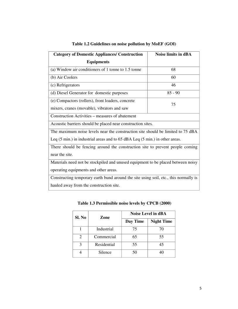
Table 1.2 Guidelines on noise pollution by MoEF (GOI)

Category of Domestic Appliances/ Construction

Equipments

Noise limits in dBA

(a) Window air conditioners of 1 tonne to 1.5 tonne 68

(b) Air Coolers 60

(c) Refrigerators 46

(d) Diesel Generator for domestic purposes 85 - 90

(e) Compactors (rollers), front loaders, concrete

mixers, cranes (movable), vibrators and saw 75

Construction Activities – measures of abatement

Acoustic barriers should be placed near construction sites.

The maximum noise levels near the construction site should be limited to 75 dBA

Leq (5 min.) in industrial areas and to 65 dBA Leq (5 min.) in other areas.

There should be fencing around the construction site to prevent people coming

near the site.

Materials need not be stockpiled and unused equipment to be placed between noisy

operating equipments and other areas.

Constructing temporary earth bund around the site using soil, etc., this normally is

hauled away from the construction site.

Table 1.3 Permissible noise levels by CPCB (2000)

Sl. No Zone Noise Level in dBA

Day Time Night Time

1 Industrial 75 70

2 Commercial 65 55

3 Residential 55 45

4 Silence 50 40

6

1.5 Objectives and Scope of this research

The objectives of this research are to measure the noise pollution levels

generated due to vehicles and machinery and also to devise a cost effective, viable

simple solution for noise attenuation.

� To determine the level of noise pollution along the noise disturbed places

� To check whether any noise attenuation is required

� To evaluate the existing noise control measures

� To suggest suitable noise attenuation measures to reduce noise pollution

� To analyse the attenuation of noise by providing the noise barrier

� To compare the efficacy of different noise barriers and suggest suitable

barrier depending upon its adaptability

� To develop noise models to predict noise pollution

� To do spectrum analysis on noise levels generated using MATLAB

software

The scope of the research conducted based on the above objectives was

recording of noise levels recorded at different noise generating sources viz.,

vehicular traffic, flour mills, construction machinery and railway stations. A

detailed study has been arrived and noise levels were recorded, compared and

presented. Attenuation of noise levels using barriers of different materials was tried

to find a cost effective noise attenuator and a comparative study made.

Noise levels due to road traffic varying spatially in different time periods are to

be measured. A comprehensive study has to be conducted with a view to understand

the noise related problem. A collective measurement technique has to be adopted

for the accurate determination of the acoustical environment of an area and source

of noise generation. The noise levels are proposed to be recorded by conducting

onsite measurements of noise levels using noise meters for a period of 8 hours and

all the values are logged. The noise levels are to be used for calculating equivalent

noise level and compared with the CPCB and MoEF guidelines. At all places of

study it was found that the noise levels measured were above the acceptable

standards. Hence an urgent need to control the noise pollution and to attenuate noise

with cost effective simple solutions is necessitated in developing countries like

India. The study also covers a review of the existing control measures and suggests

7

improvement such as barrier provision to attenuate noise levels. Three different

types of noise attenuating barriers viz., thatched shed, concrete cubicles and fly ash

cubicles are proposed to be constructed on a traffic road. Noise levels are to be

measured within and outside the barriers and a comparative study is to be carried

out. The reduction in noise levels due to the provision of barriers is to be

established.

It is also proposed to address the problem of low frequency noise as people’s

hearing sensitivity varies from one individual to another that is often the case that a

low frequency noise which is heard by one person is not heard by another. An A-

weighting network capturing low frequency noise is to be utilised to analyse

frequency spectrum through FFT (Fast Fourier Transform) analyser to arrive a band

spectrum displaying the amount of LFN generated in all sources of noises.

8

CHAPTER 2

LITERATURE REVIEW

2.1 General

Human needs for transportation has always been evolving and growing with

time. In early days man had depended on himself and animals for carrying on

transportation tasks. According to history, wheeled vehicles had existed some thousand

years ago. Presently solid wheeled vehicles combined with automatic controls have

come into existence. India seems to be one of the lands where roads received

considerable attention quite early to serve the needs for the transportation requirements.

Road development is very important for economic development of any region.

In order to increase the efficiency of the transportation system new roads are laid and

existing one are being improved.

Traditionally road work is labor intensive and requires deployment of heavy

machinery. Well mechanized operations are carried out in metropolitan areas. Since

road projects are generally intended to improve the economic and social well being of

people increased road capacity and improved pavements can lower the costs of vehicle

use and also reduce the transportation costs for both freight and passenger traffic.

With all the important aspects of road projects it has significant positive aspects

and negative aspects on nearby communities and the natural environment. Primary

disturbance to the natural environment may include aesthetic, air quality, circulation,

traffic pattern, social disturbance, soil erosion, noise hindrance, water quality, and wild

life, etc. There are other secondary effects such as change in land use, social

development, mass movement, etc.

Environmental impact arising out of any project falls in four categories

• Direct impact

• In direct impact

9

• Cumulative impact

• Post impact

The above impacts are further categorized according to nature as

• Positive and negative impact

• Random, predictable, and sensitive impact

• Local, wide spread impact and adverse impact

• Temporary, permanent and tertiary impact

• Short and long term impacts

Impacts are sometimes easier for inventory, assessment and control, since the

relationship between cause and effect is usually obvious. In some cases impacts are

more difficult to measure and ultimately important to profound for consequences. Over

time they can affect larger geographical areas of environment than anticipated.

To qualify environmental impact by the type of effect they have on the environment

is not sufficient. Impact must also be categorized according to their seriousness. The

most damaging and longest lasting impact will obviously be the first to be avoided and

mitigated.

Additionally there can be effects on vegetation, water flow and siltation. Road work

in build up areas can be a source for dust and noise. The most pronounced effects of

road transport were exhaust gases and noise emitted by vehicles. In metropolitan areas

there is a high level of air pollution as well as noise pollution along road ways.

Most of the impacts can be mitigated through proper engineering design and applying

environmentally appropriate construction methods.

To mitigate these adverse impacts a range of measures are available. But how far those

measures are successful is to be researched (Dasarathy and Thandavamorthy 2013a).

It is now becoming important that environment friendly measure is mandatory.

The consequences are to be analyzed at the planning stage and it has to be monitored

continuously. Now a day, post impact study is given less important after completion

and commissioning of any project. This thesis will focus on a particular source of

environmental pollution like noise pollution and compare with the help of publications

in the literature. The researcher is able to demonstrate how far the mitigating measures

10

which are the primary functions for Environmental Impact Assessment studies are

insufficient.

2.2 Purpose of literature review

In this chapter an extensive review of literature has been carried out with regard

to noise pollution, causes, and sources for different aspects. These reviews will

emphasis on all formations relating to environmental considerations for the occurrence

of any noise pollution.

To qualify noise pollution by the type of effect they have on the environment is

not sufficient. Impact must also be categorized according to their seriousness. The most

damaging and longest lasting impact will obviously be the first to be avoided and

mitigated. The collection of literature ranges from the year 1986 to the year 2014. The

references are arranged in a systematic manner to assist realization of the objective of

the study. Even though some of the references are not directly related to the thesis but

are still included because of their usefulness and relevance.

Extensive survey of literature in terms of research reports, technical papers, journal

articles, conference proceedings, websites and brochures containing theoretical

calculations, experimental calculations, field applications and practical stimulations of

barriers was carried out.

2.3 Review of published papers

The published papers available in the open literature are collected and categorized

based on the following headings

• Noise pollution defining the noise and explaining about noise pollution causes,

effects and mitigation measures.

• Noise pollution and its health effects

• Noise from different sources

• Noise generation from construction operations

• Noise guidelines from competent authorities

• Noise control measures

• Noise barriers forms and types of barriers

11

• Noise prediction models

• Noise spectrum analysis for frequency distribution

The policy section of the Environmental Policy Branch Environment Protection

Authority (Report 1999) on Environmental criteria for road traffic noise from noise

report shows that there are needs for programs to complement strategies that are geared

towards reducing motor vehicle use with more effective ways of managing existing

levels of traffic noise, through influencing the nature of road design, road use and

development adjacent to roads. Maximum noise levels during the night-time period (10

pm – 7 am) should be assessed to analyze possible affects on sleep. The assessment

should encompass the likely maximum noise levels due to road traffic, the extent to

which these maximum noise levels exceed ambient noise levels, and the number of

noise events from road traffic during the night on an hourly basis for a ‘typical’ night.

Noise levels that are attributable to sources other than road traffic, including sirens on

emergency vehicles, should be discarded. When describing the measurement and

analysis procedures used in any monitoring program, details of the method used to be

given to determine maximum noise levels.

Noise pollution levels in Visakhapatnam City (India) have been reported by Vidya

Sagar and Nageswara Rao (2006). Visakhapatnam is an industrial and sea port city

located on the east coast of India. A hospital (RCD hospital), residential area (Lawson’s

Bay Colony), traffic zone (Jagadamba junction, Andhra Pradesh State Road Transport

Corporation Complex junction and Seethammadhara junction) and industrial zone (sea

port) were chosen to monitor the noise levels. The observed noise level at RCD hospital

was more than 10 dBA at any time. The background noise at Santhi Ashram was

approximately 3 dBA less at night time and 2 dBA less at day time compared to ambient

air quality noise standards (AAQNS) for silent zone. The ambient air quality noise levels

(AAQNL) at traffic junctions were 5 dBA or more than those prescribed by AAQNS for

commercial zone and most of the values were found in the range of 80 + 10 dBA, among

which 75% values were found in the range of 110 + 10 dBA. AAQNL near port were

found in the range of 5 to 10 dBA positive shifts on AAQNS due to conveyor operation.

The AAQNL were alarming even in the absence of conveyor system, indicating the

impact of vehicular traffic. Remedial measures were suggested separately for each

situation.

12

A Draft Comprehensive Plan to Tackle Road Traffic Noise in Hong Kong the

Digest Environmental Protection Department (Anon. 2006a) Hong Kong is one of the

densest cities in the world with most of the 6.9 million people being housed in 225

square kilometers of development. Similar to other metropolitan cities, Hong Kong is

facing significant road traffic noise problems. Excessive road traffic noises deteriorate

the quality of life. Similar to other metropolitan cities, many residents in Hong Kong

are exposed to high level of road traffic noise. Although the Government has taken

many proactive actions, road traffic noise still remains the most severe environmental

noise problem. The Government would continue to adopt a "balanced, integrated,

proactive and transparent" strategy in tackling road traffic noise. All relevant

stakeholders would be consulted to conduct necessary feasibility studies and seek

funding and resources to develop and implement the proposed enhanced measures to

tackle the road traffic noise problems. Support from all stakeholders and in partnership

with them is crucial in this common endeavor to pursue a satisfactory noise

environment

Assessment of noise quality in Bolpur- Santiniketan areas of India was made by

Padhy and Padhi (2005). Noise is a prominent feature of the environment including noise

from transport, industry and neighbors. An important part of noise assessment is the

actual measurement of the noise levels. Continuous Leq measurement during day time

(0600 – 2100 hr) was carried out in residential, commercial and silence zone location of

Bolpur-Santiniketan areas during June-December, 2005. The results show that the noise

pollution in the city is wide spread throughout most of its area. The noise in this area is

composite in nature. Public participation, education, traffic management and structural

designing play a major role in noise management.

Gwalior is an important historical city of Madhya Pradesh, India. Rising level of

transportation mainly by road vehicles i.e., tempos, rickshaws, four wheelers, two

wheelers and heavy vehicles is one of the major source of augmented noise pollution in

Gwalior. The ambient noise level was measured by using Sound Level Meter SL- 4010.

The highest noise level was recorded at commercial area like railway station and

accordingly a maximum of 119.2 dBA at Batmorar and 92.7 dBA at Thathipur followed

by residential zone a maximum of 69.8 dBA at Pinto Park and 77.2 dBA at Lascar and

silence zone 64 dBA at Madhav dispensary and 65.8 dBA at Jiwaji campus were found.

13

The noise level values far exceeded the standards set by the CPCB. A cross-sectional

study on the basis of questionnaire was carried out the results of which revealed that

100% of the respondents were not wearing ear protective equipments. Noise annoyance,

headache, speech interference, etc., have been reported by various shopkeepers. Various

mitigation measures have been suggested to keep the noise level within the prescribed

standards (Wani and Jaiswal 2010).

Singh and Davar (2004) in their paper on Noise pollution - sources, effects and

control describe the life of the people. Cross-section surveys of the population in Delhi

State points out that main source of noise pollution are loudspeakers and automobiles.

However, female population is affected by religious noise a little more than male

population. Major effects of noise pollution include interference with communication,

sleeplessness, and reduced efficiency. The extreme effects e.g., deafness and mental

breakdown neither is ruled out. Generally, a request to reduce or stop the noise is made

out by the aggrieved party. However, complaints to the administration and police have

also been accepted as a way of solving this menace. Public education appears to be the

best method as suggested by the respondents. However, government and NGOs can

play a significant role in this process.

Chanhan and Pande (2010) deal with monitoring of noise pollution at different

zones of Dehradun, Uttarakhand, India. Exposure to high level of noise may cause

severe stress on the auditory and nervous system. Transportation and horn used in

vehicles are the major sources of noise pollution in Dehradun City.

The assessment of noise pollution can be made through measurements which,

however, are restricted to a limited number of points. The simulation of the sound waves

propagation enables the study of a whole region in respect to the expected sound pressure

levels as a result from existent sound sources. Of course, in order to perform a meaningful

simulation, the environmental properties as well as the characteristics of the sound sources

must be modeled. The results obtained may be gathered and presented graphically as in a

so called noise map. Actual measurements are used to verify and adjust the simulation to

the real situation. Noise mapping techniques together with standards for the calculation of

noise propagation are powerful tools to aid urban planners in correctly applying noise

abatement measures in an economically feasible way. Nevertheless, the results of such

mappings rely on a great amount of data, location and strength of noise sources, ground

14

geometry, location and geometry of buildings, etc. This work also discusses the sensitivity

of the obtained simulated noise levels to the quality and precision of the geometric data

available. Actual measurements are however, needed only to verify the model Fernando

and Pinto (2010).

A study and comparison of the noise dose on workers in a small scale industry in

West Bengal, India, was conducted by Sen and Bhattacharjee (2008). This paper refers to

a study and effect of noise dose in a small scale manufacturing sheet metal industry

situated in West Bengal of India. Different noise related data were taken from

individual machine and compared with the different noise related variables with Leq,

Lav, LAE and TWA (Time weighted average). Noise induced hearing loss (NIHL),

which is creating highly environmental pollution, causes the leading occupational

disease. For the development of age related hearing loss, it creates a major contribution.

A noise related hearing loss reduction for workers is proposed in this paper.

Agbalagba et al (2013) conducted a survey on noise pollution levels in four

selected sawmill factories in Delta State. The physical measurement assessed the noise

level of different machines in the factories and the background noise levels were

measured at 50 meters away from the factories. A mean level of machine noise

pollution (and background noise level) of 103.77 ± 4.71 dBA (78.25 dBA), 96.55 ±

1.48 dBA (72.08 dBA), 99.02 ± 3.20 dBA (72.54 dBA), 99.97 ± 3.66 dBA (79.89 dBA)

was recorded in Ozoro, Ughelli, Warri and Sapele, respectively. These recorded values

show that the noise levels in the four factories investigated are well above the federal

environmental protection agency (FEPA) recommended maximum permissible limits

for an industrial environment. This may cause hearing impairment and some

psychological effect like susceptibility to mistake, irritation, and sleeping and social

discomfort among staff and resident living in close vicinity to these factories. This is

further affirmed by the social survey which revealed the level of social discomfort and

health menace caused by machines noise from the factories on the workers and those

residing close to these factories. Recommendations were therefore made to control, and

abate this health threatening pollution effects.

Ehrampoush et al (2011) conducted a noise pollution study in Yazd city, Iran.

The aim of the study was to determine noise pollution in different parts of Yard’s city in

2010 and to compare them with current standard levels. A total of 135 samples were

15

obtained from both residential and commercial areas according to the ISO1996-2002

method in order to measure noise pressure levels. Locations included 10 streets and 5

squares of city and the measurement times were considered in the morning, afternoon

and evening. Noise level was determined in A-weighted by sound level meter model

2232. Results showed that the rate of background noise in Yazd city was high as it was

71.24 ± 4 dBA, 66.23 ± 7 dBA and 60.3 ± 4 dBA in the L10, L50 and L90, respectively.

The mean level of maximum noise pressure was 74.3dBA and mean Leq was 66.7dBA.

Comparing the noise level obtained in the present study to the standard level, it can be

obviously concluded that the noise levels are higher than that of acceptable levels in

most parts of the city. So, different preventive counter measures such as increasing

public awareness through educational programs and technical controls for the future

development of the city are crucial.

Mangalekar et al (2011) conducted a study of noise pollution in Kolhapur city,

Maharashtra, India. Kolhapur city is a district place in the state of Maharashtra, India

with population of 5,49,283. It is one of the emerging industrial and commercial cities

of Western Maharashtra. Problems of pollution along with noise pollution are

increasing with time, especially, due to the increase in the number of vehicles for

transportation. In the present study, continuous monitoring of noise levels Leq dB (A)

was carried out for three days in the month of December, 2011 at six different sites

within the Kolhapur city. On the basis of location, these sites were grouped into

industrial, commercial, residential and silent zones respectively. The average noise

level at industrial, commercial, residential and silence area were 74.28 dBA, 65.52

dBA, 58.88 dBA and 50.02 dBA, respectively. The results showed that there is an

enhanced pressure of noise at all sites due to increase in the number of vehicles and

facilities of transportation. All the sites under study showed higher sound level than the

prescribed limits of Central Pollution Control Board (CPCB).

Ambient noise level monitoring was carried out by Balashanmugam et al (2013)

at various locations of the Chidambaram town of Tamil Nadu, India during September –

November 2011. The data obtained was used to compute various noise parameters,

namely, equivalent continuous level (Leq), Noise pollution level (Lnp), Noise climate

(NC), Percentile noise levels (L10, L50, L90). The comparison of the data shows that the

noise levels at various locations of the Chidambaram town are more than the

permissible limits. Vehicular traffic and air horns are found to be the main reasons for

16

these high noise levels. This study examines the problems of reduction of individual's

efficiency in his/her respective working places because of road traffic noise pollution in

Chidambaram due to rapidly growing vehicular traffic. This paper deals with

monitoring of the disturbances caused due to vehicular road traffic interrupted by traffic

flow conditions on personal work performance. Traffic volume count and noise indices

data were collected simultaneously at ten selected sites of the town. The noise level

values far exceeded the standards set by the Central Pollution Control Board (CPCB).

Traffic noise measurements as well as social survey were conducted at different

locations along the National Highway No.17 at Mangalore, India by Mohapathra et al

(2012). Noise measurements were taken at 2 min and 5 min intervals. The measured

data were analyzed in the form of Leq value. From the survey results, perception of the

people and consequently the relationships between annoyances due to traffic noise and

other variables were established among residents, general public and shop owners with

the help of correlation analysis. Three prior models were constructed based on the

strong correlation coefficient for different degree of annoyance for different parts of a

day.

The study by Banihani and Jadaan (2012) provided an evaluation of road traffic

noise pollution in the city of Amman and its effects on residents. Statistical noise index

L10 (18 hr) was measured at nine different sites throughout the city of Amman. The

British Calculation of Road Traffic Noise (CRTN) method was used to predict noise

levels at the chosen sites. The results showed that Amman was environmentally noise

polluted at the studied locations with noise levels ranging between 80.41 dBA and

83.71 dBA; thereby exceeding the maximum allowable limit of 63 dBA. The

effectiveness of noise barrier walls in reducing noise levels was investigated. Noise

barriers 5 meter high were found to be effective in reducing noise levels below the

permissible limits at all sites. A social survey was carried out to evaluate the perceived

noise impacts of road traffic noise on residents. The results of the survey revealed that

road traffic noise was a major concern for the communities living in the vicinity of

streets.

The World Health Organization (WHO) carried out an assessment of the global

disease burden from occupational noise, as part of a larger initiative to assess the impact

of 25 risk factors in a standardized manner (Report 2001). This guide was built on the

global assessment, by providing a tool for occupational health professionals to carry out

17

more-detailed estimates of the disease burden associated with hearing loss from

occupational noise at both national or sub national levels. It was complemented by an

introductory volume on methods for assessing the environmental burden of disease. The

present guide describes how to quantify the burden of disease associated with hearing

impairment from occupational noise. The following topics are described:

− Noise characteristics and their relevance to workers’ health;

− Criteria for selecting health outcomes for the burden of disease assessment;

− Methods of assessing exposure to workplace noise, for all segments of a

population;

− Relative risk data for the main health outcome of occupational noise;

− Procedures for generating a summary measure of the burden of disease from

occupational noise;

− Sources of uncertainty in disease burden estimates;

− Policy implications.

The European Environmental Agency released a report on Good Practice guide

(Anon. 2010b) on noise exposure and potential health effects. The main purpose of this

document is to present current knowledge about the health effects of noise. The

emphasis was first of all to provide end users with practical and validated tools to

calculate health impacts of noise in all kinds of strategic noise studies such as the action

plans required by the Environmental Noise Directive (END) or any environmental

impact statements. The basis of this was a number of recent reviews carried out by well

known institutions like WHO, National Health and Environment departments and

professional organisations. No full bibliography was provided but the key statements

were referenced and in the reference list, some documents were highlighted which

might serve as further reading.

Noise is a stressor of today for man’s working and living place. Therefore, the

present study by Abolhasannejad et al (2013) was conducted aiming to compare the

noise sensitivity and annoyance among the residents of Birjand old and new districts. In

this analytical – descriptive study, using Weinstein noise sensitivity scale and the seven

point scale of noise annoyance based on ISO 15666 standards the rate of noise

sensitivity was measured as one of the attitudinal factors as well as that of noise

annoyance among individuals exposed to environmental noise. The result showed that

18

the mean total score of sensitivity was 63.5 ± 16.1 dBA. The highest and lowest scores

in noise sensitivity subscales associated with “sensitive to noise” and “attitude towards

noise in residence”, respectively. No significant difference was seen between total score

of noise sensitivity in old and new district among both sexes. Between “attitude towards

noise control” at illiterate and university education levels significant difference was

observed. Also, a significant difference was seen between noise annoyance in the old

district and job. The one way analysis of variance showed a significant difference

between annoyance degrees and noise sensitivity subscales. This research clearly

showed that most of the heavy traffic areas were located in the old district. Lack of

urbanization measures has caused noise pollution and dissatisfaction among the

residents. Regarding higher degrees of annoyance in the old district, probably caused by

heavier traffic, particularly by motorcycles and narrower streets, one can reduce noise

pollution and its subsequent physical and mental disorders by eliminating old and noisy

vehicles and expanding urban green spaces.

The report of most common sources of noise in the city (2010a) provides an

understanding of noise related problems. In order to enforce this objective, the New

York City Department of Environmental Protection (DEP) and the New York City

Police Department (NYPD) share duties based on the type of noise complaint. This

booklet is designed to provide an overview of the Noise Code and some of the most

common sounds of the city.

A study on characteristics of transportation noise sources in Klang Valley,

Malaysia by Yusoff and Karim (1997) stated that they detected the level of noise

pollution due to various modes of transportation, its effect towards the environment and

to look at some of the control measures that could be adopted to minimise the impact of

the noise emitted. Noise level measurements and recording were taken at a few selected

sites in the Klang Valley. From the hourly continuous noise levels recorded for 24

hours by using the sound level meter and noise level analyser, it had been found that

these areas were seriously polluted by these noise sources. Subsequently, the Lr, Lro,

Lo and Lq noise indices were identified and determined. Simultaneously, public survey

had also been conducted to gauge the existing public attitude and degree of awareness

towards contemporary transportation noise pollution problems.

19

A quantitative approach to construction pollution management and control

based on resource leveling by introducing parameters of construction pollution index

(CPI) and hazard magnitude (hi) was proposed by Li et al (2000). Using these

parameters, a method to predict the distribution of accumulated pollution level

generated from construction operations was presented. It was suggested that if the

pollution level exceeded the allowable limit, then construction activities needed to be

re-scheduled to ‘spread’ the pollution emissions. In doing so, pollution emission was

treated as a pseudo resource, and then applied to a GA based leveling technique to re-

schedule the project activities. The authors suggested that the proposed method for

controlling construction pollution was an effective tool that could be used by project

managers to reduce the level of pollution generated from a project at a certain period of

time. This method is useful when there is no other ways to reduce the level of pollution.

However, it is necessary to point out that the method proposed here can only

redistribute the amount of pollution over project duration so that at any specific period

of time, the level of pollution will not exceed the legal limit. In order to reduce the

overall amount of pollution, other methods, such as alternative construction

technologies, new materials, have to be applied.

As per Australian Construction Agency (2007) controlling construction noise

can pose special problems for contractors. Unlike general industry, construction

activities are not always stationary and confined at one location. Construction activities

often take place outside where they can be affected by weather, wind tunnels,

topography, atmosphere and landscaping. Construction noise makers, e.g., heavy earth

moving equipment, can move from location to location and is likely to vary

considerably in its intensity throughout a work day High noise levels on construction

worksites can be lowered by using commonly accepted engineering and administrative

controls. This booklet is filled with tips for contractors and to lower the noise levels on

construction worksites. Normally, earplugs and other types of personal protective

equipment (PPE) are used to control a worker’s exposure to noisy equipment and work

areas. However, as a rule, engineering and administrative controls should always be the

preferred method of reducing noise levels on worksites. Only, when these controls are

proven unfeasible, earplugs as a permanent solution should be considered.

Sellappan and Janakiraman (2014) have showed that untreated noise levels of

generator set were 100 dBA or more. From this it was clear that generator set noise

20

mitigation was a subject of great importance. The permissible exposure level 90 dBA

was reached at 7.0 m from G1 and 10.5m from G2 generator. The noise effects from

generators can be mitigated by introducing noise reduction screens or acoustic shields

around, or provide hard barricades to exclude the employee’s entry and minimize the

exposure in noisy zone. The combined noise exposure to workers ranges from 76.2

dBA to 92.5 dBA; this represents a cautionary risk of hearing damage to 600

construction workers involved in this work area. This scenario exists in many

construction sites wherever open generators are used for power generation and seeks

implementation of an effective hearing protection and awareness program. Furthermore,

the high cost of retrofitting a site for noise reduction makes it imperative to assess noise

performance requirements early in the on-site power system design stage. Working

closely with local regulations, a consulting engineer or acoustic specialist should be

involved in achieving the sound- attenuation goals. The first part of this paper assesses

the potential noise emissions associated with two unclosed caterpillar power generators

used in a construction site. In the second part combined noise effects of generators and

other activities are studied over a 12 hr period to establish background environmental

noise levels. The study shows large number of construction workers working nearby

generators are exposed to 100 dB (A) or more noise. The chain of noise control at the

source – along the noise path or at the receiver – and what effective steps could be

taken to mitigate the noise exposure at each stage are considered.

Gilchrist et al (2003) described a deterministic model for predicting the noise

levels that could be anticipated in the vicinity of construction operations. A growing

number of construction projects were performed in congested urban areas. Often, the

surrounding community founds these projects annoying because of noise, vibration,

dust, light, and greenhouse gas emissions. This paper focuses on one type of irritant,

noise. Common noise generators on construction sites are identified, and the elements

of a generic program for mitigating construction-related noise are outlined. Mitigation

strategies including source control, path control, and receiver control are discussed The

model uses the branch method together with standard attenuation and dissipation

equations developed in the areas of transportation and industrial engineering to estimate

the instantaneous noise level around a construction site. The Monte Carlo simulation

method is used to predict 500 possible outcomes using random determination of the

operation status of the various pieces of equipment involved. The model provides a

21

decision support tool for determining the need for noise-control measures at different

receptors

IOMA’s safety directors’ report (2003) says safety professionals know that

noise is one of those “facts-of-life” hazards wherever construction is going on. (There

seems little way around it—these projects make noise). But this mindset may be

putting workers at unnecessary risk, according to experts barriers must be placed

between the noise source and exposed workers.

_ Enclose the noise source. Use a quieter noise source or reduce the noise at the

source through engineering retrofit.

_ Increase the distance between the noise source and workers exposed to it.

_ Use active noise-control equipment, such as “white noise” generators.

_ Improve the maintenance of equipment including keeping blades sharp.

_ Purchase quieter equipment when new or replacement equipment is needed.

_ Schedule the use of a noise source when the fewest workers are present.

_ Limit the dropping of materials from heights.

_ Post noise warning signs and signs that remind workers to wear noise-

protection devices.

Study by Fernandez et al (2010) states that there are several noise sources in the

construction sector that may affect the workers along the whole construction work. So,

seven different construction sites have been considered (three housing blocks, three of

single family dwellings and one warehouse), where 40 workers have been measured. In

general, it can be stated from the data achieved that the sound environment which the

construction workers are within is quite noisy and potentially harmful to health, since

the lower limit of 80 dBA is exceeded in most of the cases, and even more, the

percentage of cases that go beyond the top limit of 87 dBA is quite high Usually, three

types of actions are considered in the working procedures of the industrial hygiene to

try to control the noise: on the source (for instance by using machines with less noise

emissions and properly labeled: on the environment (for instance by using enclosures

and barriers and on the worker (essentially by using hearing protection devices).

Noise guidelines given by MoEF and supported by CPCB standards presented

ambient air quality standards for the noise pollution from the different sources. Whereas

the increasing ambient noise levels in public places from various sources, inter-alia,

industrial activity, construction activity, generator sets, loud speakers, public address

22

terms, music systems, vehicular horns and other mechanical devices have mysterious

effects on human health and the psychological well being of the people; it is considered

necessary to regulate and control noise producing and venerating sources with the

objective of maintaining the ambient air quality standards in respect of noise. All the

factors are considered in the standards formation and they are listed.

Mitigation measures against road traffic noise in elected places prepared by

Hong Kong research library (Anon. 2006b) to tackle this subject, it had been suggested

by Members that a comprehensive study should be conducted with a view to

understanding the present government policy and mechanism in determining the need

for mitigation measures and the scope of measures, including noise barriers, which can

be put in place. The study should also cover the measures and improvement works

undertaken by other densely populated urban cities under similar circumstances. As the

mitigation of traffic noise falls within the terms of reference of the Panel on

Environmental Affairs (the EA Panel) of LegCo, it was agreed that the study be steered

by the EA Panel, with all Members, in particular members of public work

subcommittee (PWSC), invited to participate in the study.

Paper by Choudhari et al (2011) has reported that noise generated from various

industrial activities can disrupt the activities. The scope and purpose of this is to control

or minimize the noise pollution and its effects on human being. Noise control method

can be classified as noise control at source, during transmission and at the receiver.

Using these noise control methods, the noise level can be reduced up to the desired

level, i.e., 70 dBA. There are two basic ways of eliminating noise at sources; through

the design or modification of machinery itself or through isolation or enclosure of the

noise source. Noise can be controlled along the path through separation of worker from

noise sources and use of barriers or reflector. Acoustical control is one of most popular

technique available for absorbing noise. This paper presents the principles of noise

control, various noise control techniques, use of noise control materials at saw mill.

According to Queens Land University of Technology, Australia (2009) in their

high‐density livability guide on noise mitigation it is important to insulate and provide

barriers against noise, and also it is important to look at measures to control noise at the

source. Managing noisy neighbors can be achieved through following good neighbor

protocols. This factsheet focuses on ways to reduce the impacts of both air‐borne and

structure‐borne noise which may undermine the livability of dwellings for residents. It

23

was recommended guidelines for the Residents, Building Managers, Designers and

Developers for managing noise in the dwelling.

According to the course conducted by Birla Institute of Technology and Science

(BITS) Pilani (Anon. 2013) identifies the sources of noise pollution. Once identified,

the reason(s) for increased noise levels to be assessed. Now, efforts shall be made to

reduce the undesired noise levels from (unwanted) noise generating sources. This leads

to marginal reduction of noise levels. It is still unbearable scientific methods of noise

control. The Statutory Regulations have prescribed the noise level exposure limits. The

public may complain to the Statutory Board for violation of noise level limits by any

noise generator. Suitable action will be taken to attenuate the noise levels and

controlling pollution. It is advisable that suitable noise control measures be taken and

reduces the interference of Statutory Board. It is high time that everyone should do this

a bit in curbing the noise pollution, which is otherwise becoming as effective as SLOW

POISONING.

As per Colin et al (2010) on engineering noise control defines the noise problem

and set a good basis for the control strategy. The following factors should be

considered:

_ Type of noise

_ Noise levels and temporal pattern

_ Frequency distribution

_ Noise sources (location, power, and directivity)

_ Noise propagation pathways, through air or through structure

_ Room acoustics (reverberation).

In addition, other factors have to be considered; for example, number of exposed

workers, type of work, etc. If one or two workers are exposed to noise pollution,

expensive engineering measures may not be the most adequate solution and

other control options should be considered; for example, a combination of

personal protection and limitation of exposure. The need for control or

otherwise in a particular situation is determined by evaluating noise levels at

noisy locations in a facility where personnel spend time.

24

As per Indian Institute of Technology Roorkee (Anon. 2012) explains the

control techniques to vehicle noise and vibration, and number of ways in which the

final sound radiation may be influenced:

�Reduction at the source of combustion forces and mechanical forces.

�Reduction of the vibration transmission between the sources and the outer

surface.

�Reduction of the sound radiation of the outer surface.

The Report on the Status of Rubberized Asphalt Traffic Noise Reduction in

Sacramento County (1993) is a joint study prepared for the Sacramento County Public

Works Agency, Transportation Division by the Sacramento County Department of

Environmental Review and Assessment and Bollard and Brennan, Inc., consultants in

acoustics and noise control engineering. The purpose of this report is to document the

effectiveness of rubberized asphalt as a traffic noise mitigation measure. Rubberized

asphalt is a bituminous mix, consisting of blended aggregates, recycled rubber and

binding agents. The rubber is often obtained from used tires. Studies conducted locally,

nationally, and internationally, have shown that rubberized asphalt can reduce the noise

pollution that is associated with roadway traffic. The specific findings of this analysis

are based primarily on a series of traffic noise level measurements conducted along the

Alta Arden Expressway, between Howe and Watt Avenues, from 1993 to the present.

The conclusions of the 6-year study indicate that the use of rubberized asphalt on Alta

Arden Expressway resulted in an average four (4) decibel reduction in traffic noise

levels as compared to the conventional asphalt overlay used on Bond Road. This noise

reduction continued to occur six (6) years after the paving with rubberized asphalt. This

degree of noise attenuation is significant, as it represents a 60% reduction in traffic

noise energy, and a clearly perceptible decrease in traffic noise. This traffic noise

attenuation from rubberized paving is similar to the results documented in several non-

related studies conducted in recent years at other locations, both nationally and

internationally (Milford et al 2012) have measured and investigated noise barriers, facade

insulation, quieter road surfaces and development and production of quieter vehicles The

purpose of this paper is to provide support when strategies, plans and positions for future

actions are discussed in order to reduce adverse noise effects more effectively. The paper

compares the effectiveness of different types of noise measures to reduce noise disturbance and

25

adverse effects in relation to the cost of the measures. The measures investigated are noise

barriers, facade insulation, quieter road surfaces and development and production of quieter

vehicles. This approach is in accordance with the traffic noise optimisation TNO report, where

it is argued that 44 % of the people are exposed to noise levels above 55 dB in total. Data from

European Environmental Agency (EEA) for agglomerations report that 51 % of inhabitants in

agglomerations are exposed to noise above Lden 55 dB. Some roads have restrictions or very low

traffic flow, and as a consequence about 10 % of the population is hardly exposed to any traffic

noise (TNO, 2011). In this paper no traffic noise exposure equate to exposure less than 40 dB.

In conclusion the authors gave handling noise at source is by far the most cost effective measure

to reduce noise annoyance.

Study by Dasarathy and Thandavamoorthy (2013b) focuses on the noise

reduction by way of providing a noise enclosure which is an apt technique to reduce

noise. This is suitable for all the places, low cost technique and does not require skilled

manpower for installation, flexible in altering the design, and can be installed in critical

places where other measures are ineffective. To address the problem of noise effects on

roads, a porous natural material called thatched leaves is used as a sound barrier and

implemented on the road side. The sound barrier is installed as a rectangular shed of

size 1.5 m × 1.2 m × 2.0 m on the side of the road. The thatched hut is a simple barrier

for noise attenuation and easily erectable. The percentage reduction of noise level

ranges from 13 to 19 by the provision of thatched leaves and it shows that the noise

level can be reduced considerably. The selected area is a suitable location because of

highly congested place the provision of noise barrier as an enclosure found to be a

suitable alternative solution for noise control measure.

The primary goal of the project report prepared by Arizona Department of

Transportation (ADOT) (Anon. 2006c) was to identify innovative noise barrier designs

that had the potential to be implemented in Arizona. The study initially focused on

gathering existing literature on noise barrier materials and designs that were non-

conventional. Literature was collected on dozens of noise barrier research projects in 12

countries around the world. The results of the previous research studies were compiled

into a matrix to assist in evaluating the various barrier designs and materials. The

evaluation matrix was used to score the barrier designs based on their acoustic

performance, as well as economic, constructability, maintenance, and aesthetic

considerations. An attempt was made to identify the processes by which ADOT selects

26

and approves various barrier designs for implementation on a project. Based on the

research and evaluation conducted for this study, it was recommended that two

innovative barrier designs be implemented in Arizona – the T-top design with

absorptive material placed on the top of the horizontal portion of the barrier and a

vertical barrier with absorptive material applied to the face of the barrier. These two

barrier designs have been shown in the available literature to reduce noise levels by up

to 3 decibels, which could reduce overall barrier heights by as much as 5 feet compared

with a conventional noise barrier of concrete or masonry block construction.

The paper presented at International conference NOISE – CON 2010 at Portugal

by António et al (2010) gave a choice for an economically ideal solution of

environmental noise barrier. It acknowledged both the cost of its main components and

the benefits it can provide, through time. An algorithm based on benefit/cost ratio

(BCR) analysis was created to achieve a systematic analysis tool. It calculated the BCR

for any potential noise barrier. The cost of a barrier could be described with known or

quantifiable parameters such as barrier height, thickness, materials, initial investment

costs, maintenance costs, replacement costs due to accidents, etc. The benefits

associated with a solution were defined by computable parameters such as sound

absorption, sound reduction, insertion loss, and even intangible parameters such as its

visual impact and environmental impact. Each benefit was weighed regarding its

importance. Using the necessary parameters it was possible to calculate the BCR of a

barrier for any number of years of life expectancy.

According to Sagarzazu (2011) gave a bibliographical revision concerning

acoustic absorbing materials, also known as poroelastics. These absorbing materials are

a passive medium used extensively in the industry to reduce noise. This review presents

the fundamental parameters that define each of the parts comprising these materials, as

well as current experimental methods used to measure said parameters. Further along,

the principle- models of characterization was analysed in order to study the behavior of

poroelastic materials. Given the lack of accuracy of the standing wave method three

absorbing materials were characterized using said principle models. A comparison

between measurements with the standing wave method and the predicted surface

impedance with the models were shown.

In the study done by Ozturk et al (2012) the barriers used for reducing traffic

noise were being examined by means of performance and construction cost. First a

27

noise prediction was made in the sample highway under certain traffic conditions in

order to determine the noise barrier requirement and the results were confirmed by

measurement. According to the noise prediction equations used in Turkey, Germany

and Canada, the effects of heavy vehicle ratio, average traffic flow speed and hourly

total vehicle quantity change on noise level and barrier requirement were examined, so

assessment could be made for highways having different traffic specifications than the

sample highway. In the continuation of the study, the working principle of noise

barriers and effects of barrier position and height on reducing noise were researched in

order to determine the construction costs of barriers in Turkey and Canada at different

heights and made from different materials. All calculated or observed results showed

that noise barrier construction was necessary and 3 m tall barrier could not perform the

desired noise reduction at all distances while 5 and 7 m tall barriers could. It was

concluded that the actual noise reduction performance was not defined by the surface

mass of used material but by the height of the barrier and the related distances.

Mutairi et al (2009) gave a model by a detailed process which involves the

following steps. Problem identification: The problem of urban traffic noise pollution is

universal and in the past few decades it has grown to the point that it has become a

major concern for both the public and the policy-makers. Approach: In a

comprehensive 18 month research project, traffic-generated noise was monitored at 47

roadway locations in fourteen districts in metropolitan Kuwait in 2004-2005.

Simultaneously with noise, traffic flow variables of volume-by mix and traffic speed

were also measured. Measurements of noise and traffic flow variables were performed

for a period of 20 min at each location, repeated 3-5 times, during peak and off-peak

hours to account for time-fluctuation of these variables. At each district, a sample of

freeway, arterial, collector and local residential streets were included in the noise and

traffic flow monitoring plan. In addition to the analysis of noise, flow and their

interrelationships, two models-regressions and the traffic noise model, were employed

to predict noise pollutions from traffic. Results: Findings indicated that traffic noise is

at or above, the standard outdoor limits in most locations and especially at arterial

roadways and freeways. Recommendations concerning measured to improve the

problem of urban traffic noise pollution in Kuwait are also made. Conclusion: Findings

of this research project had shown that level of traffic generated noise pollution in

Kuwait urban area is high enough to adversely affect the welfare activities and

28

productivities of its residents. With the rapidly growing rate of infrastructural

development and unplanned urban land-use change, it is almost certain, that problem of

urban traffic noise pollution will soon assume a critical dimension and will be a cause

of increasing concern for both public and responsible policy-makers. The quality of

urban life will undoubtedly be adversely affected.

Karantonis et al (2008) provided an update of information presented in a paper

presented at the AAS Acoustics 2008 conference in Geelong, Victoria. In particular this

paper presents results of traffic noise modeling using CadnaA and SoundPLAN and

compares both to noise measurements for three large recent road projects in NSW.

CadnaA is a well known and internationally accepted noise modeling package, and its

acceptance and use in Australia amongst acoustic professionals is growing fast. To

assist the Australian acoustical profession, the appropriateness and accuracy of CadnaA

under Australian conditions is currently being verified, and this paper presents actual

project results for this purpose. Unlike CadnaA, the SoundPLAN noise prediction

model is extensively used in Australia, particularly for road traffic noise predictions,

and has been recognized and accepted nationally by various regulatory authorities

including the major road authorities and environmental agencies. The aim of this paper

was to provide additional comparative data for predicted traffic noise levels using the

Calculation of Road Traffic Noise (CoRTN) algorithms as implemented by

SoundPLAN and the CadnaA noise models for three large recent road projects in NSW.

These three projects offered features and characteristics that differed significantly from

the projects reported in the 2008 paper. Results from this study re-confirmed that the

CadnaA noise modeling package was accurate and effective for modeling road traffic

noise in Australia.

Fan Dan Qun et al (1986) gave the medium term prediction of noise and

evaluation of noise pollution in “microscopic” way using computer and was a new

research work in China. In this paper, some investigations including the methods of

prediction and evaluating urban traffic pollution have been reported. Models for

vehicles flow and propagation of noise in urban areas have been setup. Finally a set of

computer programs for these purposes was given. Models and computer programs had

been tested in more than 70 cities of China. It was proved that they could be used in

medium and long term prediction of urban traffic noise pollution in China and they

were of great values in evaluating the extent of urban traffic noise pollution.

29

Models were developed by Golmohammadi et al (2007, 2009). Background:

The recognition of road traffic noise as one of the main sources of environmental

pollution had led to develop models that enabled to predict noise level from

fundamental variables. Traffic noise prediction models were required as aids for

designing roads and highways. In addition, sometimes were used in the assessment of

existing or envisaged changes in traffic noise conditions. In this paper a statistical

modeling approach had been used for predicting road traffic noise in Iranian road

conditions. Methods: The study was performed during 2005-2006 in Hamadan city, in

the west of Iran. The data set consisted of 282 noise measurements. The entire data set

was utilized to develop a new model for Iranian condition using regression analysis.

Result: The developed model had twelve explanatory variables in order to achieve a

proper fit for measured values of Leq (R2 = 0.913). Conclusion: The proposed road

traffic noise model could be effectively used as a decision support tools for prediction

of traffic noise index of Leq(30 min) in Iran's cities.

Modeling free flowing vehicular traffic noise was developed by Sooriyaarachchi

and Sonnadara (2008). Traffic noise of 650 vehicles classified into 8 vehicle classes

was measured in several locations within the Western Province of Sri Lanka in order to

extract the necessary coefficients to develop a road traffic noise prediction model. The

model was developed to predict the traffic noise generated from free-flowing vehicles

in roadways. Traffic flow data used for constructing this model was limited to vehicle

noise, vehicle class, vehicle speed and the distance from the traffic flow line. It is

shown that the predictions could be made within ±11 dBA accuracy with respect to the

actual experimental observations. Microsoft .Net® platform was used for the

development of the traffic simulator based on the model parameters.

Evaluation and mitigation of road traffic noise in Amman, Jordan done by

Jadaan et al (2012, 2013) provided an evaluation of road traffic noise pollution in

Amman, the capital of Jordan through measuring and predicting the statistical noise

index L10 (18 hr) at selected sites using the British calculation of road traffic noise

(CRTN) method after validation. The measured and future noise levels were found high

and exceeded the maximum allowable limit of 63 dBA at all survey sites calling for the

need to apply mitigation measures. The effectiveness of noise barriers in reducing noise

levels was investigated and 3-5 m noise barriers were found appropriate.

30

The investigation of noise attenuation by plants and the corresponding noise –

reducing spectrum by Fan et al (2010) stated as noise pollution was becoming more and

more serious, many researchers were studying the noise attenuation effect provided by

plants. This article examines six kinds of evergreens as research subjects so as to

compare the different arrangements and densities of plants and their effect on noise

attenuation. The authors studied the relationship between each of the plant’s

characteristics (the characteristics include leaf area, leaf fresh weight, leaf tactility, and

leaf shape) and their average relative noise attenuation. The authors then generated the

noise reducing spectrum of the six plants. The results showed that there was a notable

difference in noise reducing effects for low frequency and high frequency when plants

were arranged differently. Also every plant demonstrated a specific noise reducing

spectrum. By quantifying noise attenuation species to achieve the mutual benefits of

plant varieties and establish an ecotype sound barrier model with effective density and

arrangement.

Proposed criteria for the assessment of low frequency noise disturbance by

Moorhouse et al (2005) was to recommend a method for assessing low frequency noise

(LFN), suitable for use by Environmental Health Officers (EHOs) in the UK. A general

introduction to LFN was given, in which it was argued that a method of assessment was

needed both from the sufferer’s point of view, because there is currently not much to

protect them against LFN, and from the Environmental Health Officer’s point of view,

where guidance is needed in determining whether a nuisance exists. Criteria already in

use in Germany, Sweden, Denmark, the Netherlands and Poland were reviewed and

compared. Experience from these countries in applying the criteria was also reviewed,

and was found to be generally positive. A complementary set of field and laboratory

studies was conducted in order to establish the best form for an assessment method. In

the field studies, eleven cases of reported LFN were investigated, as well as five control

cases where no complaints about LFN had been received. Analysis of recordings made

over three to five days at each location distinguished three groupings: positively

identified LFN, unidentified, and marginal. Three cases were positively identified,

meaning that the various national criteria were exceeded and there was correlation

between the resident’s logged comments and the LFN level. Five cases were

unidentified: the criteria were generally not exceeded, (except perhaps by traffic noise),

and there was a lack of correlation between comments and noise levels. Three cases

31

were marginal in that the LFN was marginal with respect to the criteria and did not

correlate with comments. It was concluded that the criteria were successful at

distinguishing cases where an engineering solution could be applied from those where

no such solution could be found.

Noise prediction simulation and noise reduction technology at low-frequencies

by Kaneuchi and Nishimura (2011) developed a noise prediction simulation and a

noise-reduction technology which could be used for low-frequency noise whose

propagation was difficult to predict and to reduce. For developing a method of noise

prediction simulation, the validity of the geometrical acoustic method and the wave

acoustic method was evaluated and confirmed. The interference mainly occurs near a

wall and in enclosed space at low frequencies. The wave acoustic method could be used

in the situation where the interference was dominant. It was confirmed that the

environmental noise impact of gas equipment could be predicted by using the

geometrical acoustic method and the wave acoustic method as the situation demands.

Additionally, for reducing the low-frequency noise in three-dimensional space, an ANC

system whose second sound source was set next to the noise source was developed.

Although its noise-reduction effect was restricted to the frequencies in the range of 20

Hz to 100 Hz, the noise at the peak frequency depending on the rotating speed of the

machine was reduced by about 15 dB. As a result of developing pre- and post-

operational measures, it became possible to suppress successfully the undesirable effect

of the noises from the system exerts on its surroundings.

The analysis with MATLAB given by Wendy and Angel (2005) was used to

define exploratory data analysis. It was an area of statistics and data analysis, where the

idea was to first explore the data set, often using methods from descriptive statistics,

scientific visualization, data tours, dimensionality reduction, and others. This

exploration is done without any pre-conceived notions or hypotheses. Indeed, the idea

was to use the results of the exploration to guide and to develop the subsequent

hypothesis tests, models, etc. It was closely related to the field of data mining, and

many of the EDA tools discussed in this book are part of the toolkit for knowledge

discovery and data mining.

According to Christoph (2001) on spectrum analysis is intended to familiarize

the uninitiated reader with the field of spectrum analysis. To understand complex

measuring instruments it is useful to know the theoretical background of spectrum

32

analysis. Even for the experienced user of spectrum analyzers it may be helpful to recall

some background information in order to avoid measurement errors that are likely to be

made in practice. In addition to dealing with the fundamentals, this book provides an

insight into typical applications such as phase noise and channel power measurements.

In low frequency noise technical research support for DEFRA Noise Programme

(Report 2001) possible causes and possible effects of low frequency noise were

described, and a procedure for investigating complaints concerning low frequency noise

is set out. Some general advice was given regarding the measurement of low frequency

noise, but a detailed measurement procedure was not given. A further detailed report on

the subject of the measurement of low frequency noise may be produced in due course.

In the field of low frequency noise and its perception, there are still a number of factors

that make it difficult to derive specific, quantitative guidelines by which to judge the

acceptability or otherwise of a given level of noise at low frequency. This document,

therefore, tries to offer suggestions which may be helpful in explaining some of the

factors most commonly affecting the outcome of investigations.

Traffic noise spectrum analysis: Dynamic modeling vs. Experimental

observations developed by Leclercq et al (2010) compares two different representations

for the assessment of urban noise frequency spectrum (i) a static one based on mean

vehicle speeds and flow rates and (ii) a dynamic one which considers vehicle

interactions along the network. The two representations were compared on their

suitability to match real on field noise levels, recorded on a three lane quite busy street.

Representations (i) falls in reproducing spectra evolves that correspond to this site. In

particular, it underestimates low frequencies, what can conceal the real impact of traffic

flow on urban sound quality. Representation (ii) greatly improves estimation. It

quarantines accurate environmental noise assessment, since it reproduces all traffic

situations that are encountered in the site. Moreover, its base structure allows for the

evaluation of spectra variations, with a good accuracy.

Tandel and Macwan (2012) carried out assessment and modeling of urban

traffic noise at major arterial roads of Surat. In India, transportation demands in urban

areas continue to increase rapidly as a result of both of population growth and changes

in travel patterns. The recognition of road traffic noise as one of the main sources of

environmental pollution has led to develop models that enable to predict noise level

from fundamental variables. Therefore, this study was carried out to generate a noise

33

prediction model and to analyze various parameters affecting road traffic noise. The

model, when validated gives quite satisfactory results. The study reveals that present

noise level at all three major arterial roads exceed the limit prescribed by CPCB. Based

on the finding, it can be said that the persons nearby these roads are exposed to

significantly high noise levels and hence necessary mitigation measures should be

adopted.

2.4 Summary of collective literatures

Findings from a large body of studies show that traffic noise causes non-

auditors' stress effects such as changes in the physiological systems, e.g., elevated blood

pressure, various cognitive deficits, poor sustained attention, memory/concentration

problems, sleep disturbances, psychosocial stress disturbance. A series of reports on

traffic noise prediction of national scope have been published, but they lack detailed

information and its application on Indian condition.

Hence, this research is to analyze the outcome of noise barriers provided and the

objectives are arrived based on the above listed literatures.

34

CHAPTER 3

3 METHODOLOGY

3.1 General

The methodology adopted includes a study of existing condition, real- time work

made to explore the general system followed in the noise pollution mitigation

measure. The methodology is presented as a flow chart in Figure 3.1

Figure 3.1 Flow Chart of Methodology

Literature Review

Objectives and Scope of research

Data Collection / Field Study and

Exposure Timings

Analysis for each Source

Results and Discussion

Conclusion

Problem Identification – Causes,

Sources, Effects, Mitigation

35

3.2 Data Collection

Data collection is the process of measuring and gathering information on

variables of interest, in an established systematic fashion that enables one to answer

stated research questions, test hypotheses, and evaluate outcomes. The data collection

component of research is common to all fields of study including physical and social

sciences, humanities, business, etc. While methods vary by discipline, the emphasis on

ensuring accurate and honest collection remains the same. The goal for all data

collection is to capture quality evidence that then translates to rich data analysis and

allows the building of a convincing and credible answer to questions that have been

posed.

Since the formal problem identified is about noise pollution a formal data

collection process is necessary as it ensures that data gathered are both defined and

accurate and that subsequent decisions based on arguments embodied in the findings are

valid. The process provides both a baseline from which to measure and in certain cases

a target on what to improve.

3.3 Field Area and Exposure Timings

The important aspect with respect to noise pollution is collecting information

about noise levels, source from where noise is created and its time of exposure. The

following are the different sources of noise to record observations.

3.3.1 Traffic noise – Noise levels were recorded at OMR (Old Mahabalipuram Road)

near Toll Plaza and SRP tools intersection, Perungalathur and Kolapakkam Road in

Chennai, Tamil Nadu, India.

• The noise levels were recorded from morning 10.00 AM to 18.00 PM at an

interval of 10 sec from Monday through Saturday at both locations.

• Total volume of vehicles for the entire period was recorded.

• Number of vehicles/Hr according to the type of vehicle such as bus, car,

two- wheeler, auto, LGV, and HGV were taken at an interval of two hours in

morning and afternoon during peak and non-peak hour.

36

• Speed of the vehicle was recorded by the way of moving car method at SRP

tools.

• Noise measurements were taken at distances of 0.90 m and 1.10 m from nearest

road border

• The height of noise measurement was 1.30 m above the road surface

3.3.2 Pedestrian noise – Pedestrian movement existed in a subway, noise level was

recorded where pedestrians were receiving the noise intensity. The noise level was

recorded near Tambaram, a suburb of Chennai pedestrian subway both inside and

outside the subway as shown in Table 3.1.

Table 3.1 Details of noise pollution from pedestrian sources and noise generation

hours

Place of noise pollution

measurement carried out

No. of hours of

survey conducted

Pedestrian location 8 hours for five days

Inside subway 8 hours for two days

3.3.3 Construction noise

Construction noise is predominant, especially cities like Chennai where construction

activity is in full swing. Construction machinery or equipments which create more

noise level during operation are selected and shown in Table 3.2.

Table 3.2 Details of noise pollution sources and noise generation hrs

Place of noise pollution measurement

carried out

No. of hours survey

conducted

Bored pile (during drilling, driving the

casing and concreting)

6 hours at two points

Vibrator (during concreting ) 45 min. at three locations

Mixer machine (when concreting work in

progress )

4 hours at two locations

Jack hammer demolishing work 6 hours at two points

Marble cutting machine for laying flooring 6 hours at two points

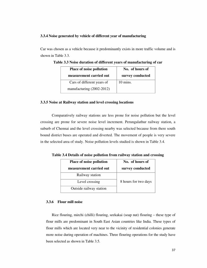
37

3.3.4 Noise generated by vehicle of different year of manufacturing

Car was chosen as a vehicle because it predominantly exists in more traffic volume and is

shown in Table 3.3.

Table 3.3 Noise duration of different years of manufacturing of car

Place of noise pollution

measurement carried out

No. of hours of

survey conducted

Cars of different years of

manufacturing (2002-2012)

10 mins.

3.3.5 Noise at Railway station and level crossing locations

Comparatively railway stations are less prone for noise pollution but the level

crossing are prone for severe noise level increment. Perungalathur railway station, a

suburb of Chennai and the level crossing nearby was selected because from there south

bound district buses are operated and diverted. The movement of people is very severe

in the selected area of study. Noise pollution levels studied is shown in Table 3.4.

Table 3.4 Details of noise pollution from railway station and crossing

Place of noise pollution

measurement carried out

No. of hours of

survey conducted

Railway station

8 hours for two days Level crossing

Outside railway station

3.3.6 Flour mill noise

Rice flouring, mirchi (chilli) flouring, seekakai (soap nut) flouring – these type of

flour mills are predominant in South East Asian countries like India. These types of

flour mills which are located very near to the vicinity of residential colonies generate

more noise during operation of machines. Three flouring operations for the study have

been selected as shown in Table 3.5.

38

Table 3.5 Details of noise pollution from flour mills and exposure time in hours

Place No of exposure time

Rice flour 2 min 5 sec Mirchi (chilli) flour 3 min 25 sec Seekakai (soapnut) flour 3 min 10 sec

3.3.7 Traffic noise with barriers

The noise barriers provided for reducing noise pollution is expensive. With costs

frequently reaching hundreds of Euros per square meter of barrier it is highly important

to choose the cost effective best solution. Four types of barriers were selected as shown

in Table 3.6.

Table 3.6 Details of traffic noise recorded using barriers

Sl.

No.

Type of

barrier Location Duration Size of barrier Nature of exposure

1

Thatched Shed

barrier

Toll Plaza

3 hours

Length 1.50 m Width 1.20 m Height 2.0 m

Open place 1 hour Shed with one layer of

thatched leaves 1 hour Shed with two layer of

thatched leaves

2

SRP tools

3 hours Open place 1 hour Shed with one layer of

thatched leaves 1 hour Shed with two layer of

thatched leaves

3

Concrete barrier

Toll Plaza

1 hour

Length 0.60 m Width 0.60 m Height 0.60m

Open place Cubicle with M30 mix concrete Cubicle with M30 mix concrete with CSP

4

SRP tools

Open place Cubicle with M30 mix concrete Cubicle with M30 mix concrete with CSP

5 Fly Ash Brick barrier

Toll Plaza

1 hour

Length 1.00 m Width 1.00 m Height 0.60 m

Open place Cubicle with fly ash bricks

6

SRP tools

Open place Cubicle with fly ash bricks

39

3.4 Equipment

An important part of noise assessment is the actual measurement of the noise

levels. The ‘A’ weighted network was used as it corresponds very closely to a person’s

hearing sensitivity. The noise level at all locations were measured with the help of HTC

make Sound Level Meter (3241 – c type II data logger) on a digital display type shown in

Figure 3.2

Figure 3.2 Noise level meter and the digital display of observation

3.5 Parameters Calculated From Primary Survey

The following noise parameters L10, L50, L90, Leq, Lnp, Lmin, Lmax, Lave, NI and

NC were calculated (Dinesh Kumar et al 2012).

L10, L50, L90 = noise level exceeded for 10%, 50%, 90% of the time in noise recording

Leq = L50 + (L10 - L90 )2/60

Lnp, = Leq + (L10 - L90 )

NI = L90 + (L10 - L90 ) – 30

NC = (L10 - L90)

Lmin, Lmax, Lave from data logger of sound level meter.

40

CHAPTER 4

4 Observations and Calculation of Parameters

4.1 Noise parameters from traffic survey at Toll Plaza and SRP Tools

Using the noise level meter traffic noise was recorded at the sensitive locations

selected as study area. The noise level is recorded using the noise level meter. The noise

level is recorded for duration of about 8 hours at both locations. The noise level was

recorded for six days from Monday to Saturday. The noise parameters such as Noise

equivalent level, noise pollution level and noise index were calculated. These are

presented in Table 4.1 and Table 4.2 for both the locations.

Table 4.1 Consolidated values of noise parameters for Toll Plaza location (dBA)

Day L10 L50 L90 Leq Lnp TNI LMAX LMIN LAVE

Monday 63.2 72.9 57.1 73.32 79.42 33.2 78.8 44.4 60.32

Tuesday 61.1 57.3 66.3 57.75 52.55 31.1 70.5 50.9 64.27

Wednesday 73.2 77.7 67.3 78.28 84.18 43.2 105.6 51.9 70.65

Thursday 73.2 77.3 62.4 79.24 90.04 43.2 105.6 51.9 74.59

Friday 71.8 59.3 55.4 63.78 80.18 41.8 83.9 44.4 61.2

Saturday 64.2 67.2 58.7 62.1 67.6 34.2 90.5 50.9 61.97

Table 4.2 Consolidated values of noise parameters for SRP tools location (dBA)

Day L10 L50 L90 Leq Lnp TNI LMAX LMIN LAVE

Monday 63.2 72.7 57.1 73.32 79.42 33.2 78.8 44.4 63.39

Tuesday 71.2 61.7 57.1 65.01 79.11 41.2 83.9 44.4 63.45

Wednesday 69.1 60.8 63.1 61.4 67.4 39.1 90.5 50.9 63.66

Thursday 63.2 72.7 57.1 73.32 79.42 33.2 79.9 44.4 63.57

Friday 71.8 69.3 71.4 69.3 69.7 41.8 83.39 44.4 64.69

Saturday 74.2 61.6 58.7 66.7 84.2 46.2 90.5 50.9 63.76

41

The observations show that noise level is in the range of about 44.4 dBA (Lmin)

to 105.6 dBA (Lmax). The noise level is 10 dBA more on Wednesday when compared

to other days at both the locations. The average noise level is in the range of 61.2 dBA

to 74.59 dBA. During 90% of the time the noise level is in the range of 55.4 dBA to

71.4 dBA. The equivalent noise level is in the range of 57.75 dBA to 79.24 dBA.

During Saturday the noise level is equivalent to a week day value which shows that the

traffic volume is existed on that day. Further recorded noise level is compared with

standards prescribed and are presented in Figure 4.1.

Figure 4.1 Comparison of noise level with the standards given by CPCB

Figure 4.1 shows Leq, Lmin, Lmax and Lave compared with the CPCB

standards. The noise level prescribed by the CPCB is 55 dBA where as the noise level

Leq is in the range of 57.75dBA to 79.24 dBA, Lmax is in the range of 70.5 dBA to

105.6 dBA, Lave 60.32 dBA to 74.59 dBA. Lmin value is in 44.4 dBA to 51.9 dBA.

This value is very close to the CPCB standards whereas this minimum value is not

reflected in L10, L50 and L90 values. This shows that the Lmin existed for very short

duration that too when the traffic is at calming.

0

20

40

60

80

100

120

Toll

Plaza

SRP

tools

Toll

Plaza

SRP

tools

Toll

Plaza

SRP

tools

Toll

Plaza

SRP

tools

Toll

Plaza

SRP

tools

Toll

Plaza

SRP

tools

MONDAY TUESDAY WEDNESDAY THURSDAY FRIDAY SATURDAY

De

cib

el

Lev

el

in d

BA

Day / Location

LMIN

LAVE

LMAX

Leq

LCPCB

42

4.2 Noise parameters from vehicles at Tambaram Subway

The pedestrians are most affected persons due to generation of noise pollution. This as a

measure, a congested location is selected to identify the level of existing noise

generated due to vehicular movement. The place selected is Tambaram, Chennai a

suburban hub for the south bound traffic from Chennai. Subway location and

surrounding place are shown in Figure 4.2.

Figure 4.2 Location of Tambaram Subway

The noise level was recorded outside the subway for 5 days and the noise level

was recorded inside the subway for two days. The noise level recorded using the noise

level meter. The noise level recorded for duration of about 8 hours at both locations.

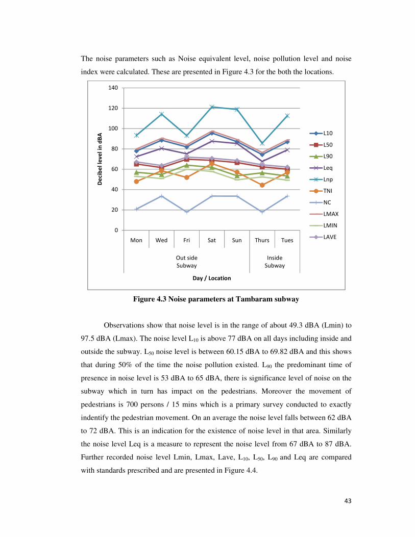
43

The noise parameters such as Noise equivalent level, noise pollution level and noise

index were calculated. These are presented in Figure 4.3 for the both the locations.

Figure 4.3 Noise parameters at Tambaram subway

Observations show that noise level is in the range of about 49.3 dBA (Lmin) to

97.5 dBA (Lmax). The noise level L10 is above 77 dBA on all days including inside and

outside the subway. L50 noise level is between 60.15 dBA to 69.82 dBA and this shows

that during 50% of the time the noise pollution existed. L90 the predominant time of

presence in noise level is 53 dBA to 65 dBA, there is significance level of noise on the

subway which in turn has impact on the pedestrians. Moreover the movement of

pedestrians is 700 persons / 15 mins which is a primary survey conducted to exactly

indentify the pedestrian movement. On an average the noise level falls between 62 dBA

to 72 dBA. This is an indication for the existence of noise level in that area. Similarly

the noise level Leq is a measure to represent the noise level from 67 dBA to 87 dBA.

Further recorded noise level Lmin, Lmax, Lave, L10, L50, L90 and Leq are compared

with standards prescribed and are presented in Figure 4.4.

0

20

40

60

80

100

120

140

Mon Wed Fri Sat Sun Thurs Tues

Out side

Subway

Inside

Subway

De

cib

el

lev

el

in d

BA

Day / Location

L10

L50

L90

Leq

Lnp

TNI

NC

LMAX

LMIN

LAVE

44

Figure 4.4 Comparison of noise level with standards

Figure 4.4 shows that the noise level Lmin is very close to the value given by CPCB

standards. The predominant time of survey shows that noise level existed at all time.

The Leq level was 24.52 dBA more than the CPCB standards. The pedestrians are

subjected to severe noise injection due to vehicular movement throughout the day. Also

there is substantial presence of hawkers near the subway where there are about 75

hawking shops in the vicinity. Approximately about 125 persons are facing the severity

of the noise during the entire day due to traffic. They also spend considerable time of

the day in selling their commodities in this environment of noise pollution.

4.3 Construction noise and noise parameters

The disturbance in terms of severity of noise caused during the construction

process and their impact vary depending on the nature of the activities being performed,

the equipment being used, and the physical nature of the surrounding environment i.e.,

urban area versus green field conditions Gilchrist et al (2003).

Controlling construction noise can pose special problems, at the same time,

there have been not many studies related to pollution control in construction sites. There

have also been some studies engaged to the quantitative measurement and effective

0

20

40

60

80

100

120

Mon Wed Fri Sat Sun Thurs Tues

Out side

Subway

Inside

Subway

de

cib

el

lev

el

in d

BA

Day / Location

L10

L50

L90

Leq

LMAX

LMIN

LAVE

LCPCB

45

control of construction pollution, using methods such as life-cycle costing; efficient

energy consumption; reduction, reuse, and recycle of construction and demolition

material/debris; degradation and abatement of construction noise and dust; and

environmental impact assessment Li et al (2000), Hassan et al (2012) and Transit noise

and vibration assessment (2000). Construction noise makers, e.g., heavy earth moving

equipment, jack hammer, marble cutting machine, mixer machine operation and

vibrator machines are taken as examples for this study.

4.3.1 Mixer Machine Operation

The operation of mixer machine shown in Figure 4.5 is manual and a person

will be used to operate. The mixer machine is used for concreting works which

completes in a day of work. Usually in residential construction and large construction

involving huge quantity of concrete, site mixer machine for concreting is preferred. The

loading of ingredients for mixing components is carried by the laborers associated with

the work. The mixer machine is usually operated for middle level construction sites and

is predominant in rural areas and suburban areas. The operation selected for the study

purpose is a multi-storeyed and residential building construction site. The operation

considered is 4 hours during casting of concreting. The noise parameters calculated are

presented in Figure 4.6.

Figure 4.5 Mixer machine in operation

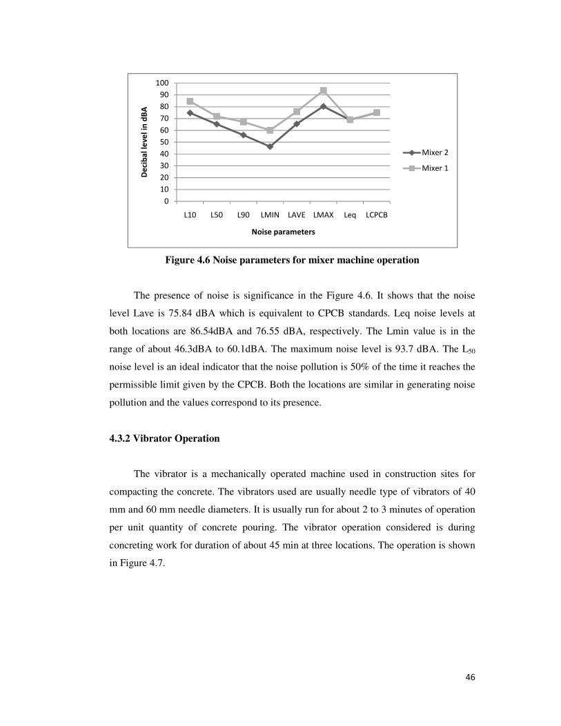
46

Figure 4.6 Noise parameters for mixer machine operation

The presence of noise is significance in the Figure 4.6. It shows that the noise

level Lave is 75.84 dBA which is equivalent to CPCB standards. Leq noise levels at

both locations are 86.54dBA and 76.55 dBA, respectively. The Lmin value is in the

range of about 46.3dBA to 60.1dBA. The maximum noise level is 93.7 dBA. The L50

noise level is an ideal indicator that the noise pollution is 50% of the time it reaches the

permissible limit given by the CPCB. Both the locations are similar in generating noise

pollution and the values correspond to its presence.

4.3.2 Vibrator Operation

The vibrator is a mechanically operated machine used in construction sites for

compacting the concrete. The vibrators used are usually needle type of vibrators of 40

mm and 60 mm needle diameters. It is usually run for about 2 to 3 minutes of operation

per unit quantity of concrete pouring. The vibrator operation considered is during

concreting work for duration of about 45 min at three locations. The operation is shown

in Figure 4.7.

0

10

20

30

40

50

60

70

80

90

100

L10 L50 L90 LMIN LAVE LMAX Leq LCPCB

De

cib

al

lev

el

in d

BA

Noise parameters

Mixer 2

Mixer 1

47

Figure 4.7 Vibrator machine in operation

The noise is generated from the motor attached with the needle which in turn

rotates for compaction. The operator is bound to start, run for few minutes and stop

frequently. This operation is done by laborers present in the work place and in turn they

receive the amount of noise generated from it. The noise level is recorded and the noise

parameters are presented in Figure 4.8.

Figure 4.8 Noise parameters for vibrator machine operation

0

20

40

60

80

100

120

L10 L50 L90 LMIN LAVE LMAX Leq LCPCB

de

cib

el

lev

el

in d

BA

Noise parameters

Vibrator3

Vibrator2

Vibrator 1

48

The noise level Leq is 71.12 dBA and 90.31 dBA, respectively. The noise level is

reaching the permissible limit mentioned by the CPCB which is 75 dBA. Here the noise

generation existed in the few hours of operating simple machinery like vibrator needle

in construction. The Lmax noise level is 81.1 dBA and 98.3 dBA shown in Figure 4.8

and reaches the peak point equivalent to CPCB standards.

4.3.3 Piling Operation

Multi-storeyed construction nowadays opts for foundation using piles. The

operation of piling is done through manual or machinery. Manual operation does not

require sophisticated equipments, whereas the mechanical operation requires full

fledged machinery arrangements for piling operation that too when the depth of

foundation exceeds more than 10 m it is always preferable to go for driven piling

operation. During driven piling operation noise generation is enormous and this

operation considered as a noise source for evaluation. The piling operation considered

is shown in Figure 4.9(a) and Figure 4.9(b).

Figure 4.9(a) Driven piling operation

49

Figure 4.9(b) Concreting of driven pile

The study area considered is a high rise building near Chennai. The piling

operation is a multiple stage process wherein it involves staging, erection of jig,

centering, driving operation, insertion of casing with bentonite solution, reinforcement

erection, pouring of concrete, and finally disassembly of entire jig arrangements. The

entire operation will have duration of about 6 to 7 hours. During the entire duration of

operation the machine will be in running condition and the noise generation is

enormous. Even though the operation and process will have minimum labour

involvement but the surrounding area for a radius of 20 m will have noise generation.

The noise level meter is placed during the entire operation and the noise is recorded at

two piling points. The noise level observed, recorded and noise parameters are

calculated and are presented in Figure 4.10.

Figure 4.10 Noise parameters for piling operation

0

50

100

150

L10 L50 L90 LMIN LAVE LMAX Leq

De

cib

al

lev

el

in d

BA

Noise parameters

Pile 2

Pile 1

50

The noise level recorded shows that the Lmin noise level is 72 dBA to 78 dBA.

The noise level is maximum of 119.9 dBA, where as the Lave is 100.46 dBA. This

shows that the noise level is predominant. During the piling operation, 90% of its

timing the noise level is 82 dBA. The generation of noise is from the attached machine

and the hydraulic operation involved in the process. The noise level generated is

uniform, and during the entire operation of one piling the noise is predominantly

exposed. The noise generation for the entire duration of piling is shown in Figure 4.11.

Figure 4.11 Variation of pile operation in a day

The Figure 4.11 represents the noise level with an amplitude in a range of 92

dBA to 110 dBA. Thus, the piling is a source of severe noise generation and it creates

pollution. The piling operation is carried out in open stream and the dissipation of noise

is minimal that shows that the severity of noise.

4.3.4 Marble cutting operation

The process of marble cutting occurs during laying of marbles in the flooring.

This operation is tedious because the marble plate will come in an irregular shape and

the person laying the plate will fine tune to accommodate by simply using a tool for

cutting. This operation generates louder noise. The laborers working near the marble

cutting operation and the process is shown in Figure 4.12.

0

20

40

60

80

100

120

140

00

:05

:10

00

:18

:50

00

:32

:30

00

:46

:10

00

:59

:50

01

:13

:30

01

:27

:10

01

:40

:50

01

:54

:30

02

:08

:10

02

:21

:50

02

:35

:30

02

:49

:10

03

:02

:50

03

:16

:30

03

:30

:10

03

:43

:50

03

:57

:30

04

:11

:10

04

:24

:50

04

:38

:30

04

:52

:10

05

:05

:50

05

:19

:30

05

:33

:10

05

:46

:50

de

cib

el

lev

el

Time Duration

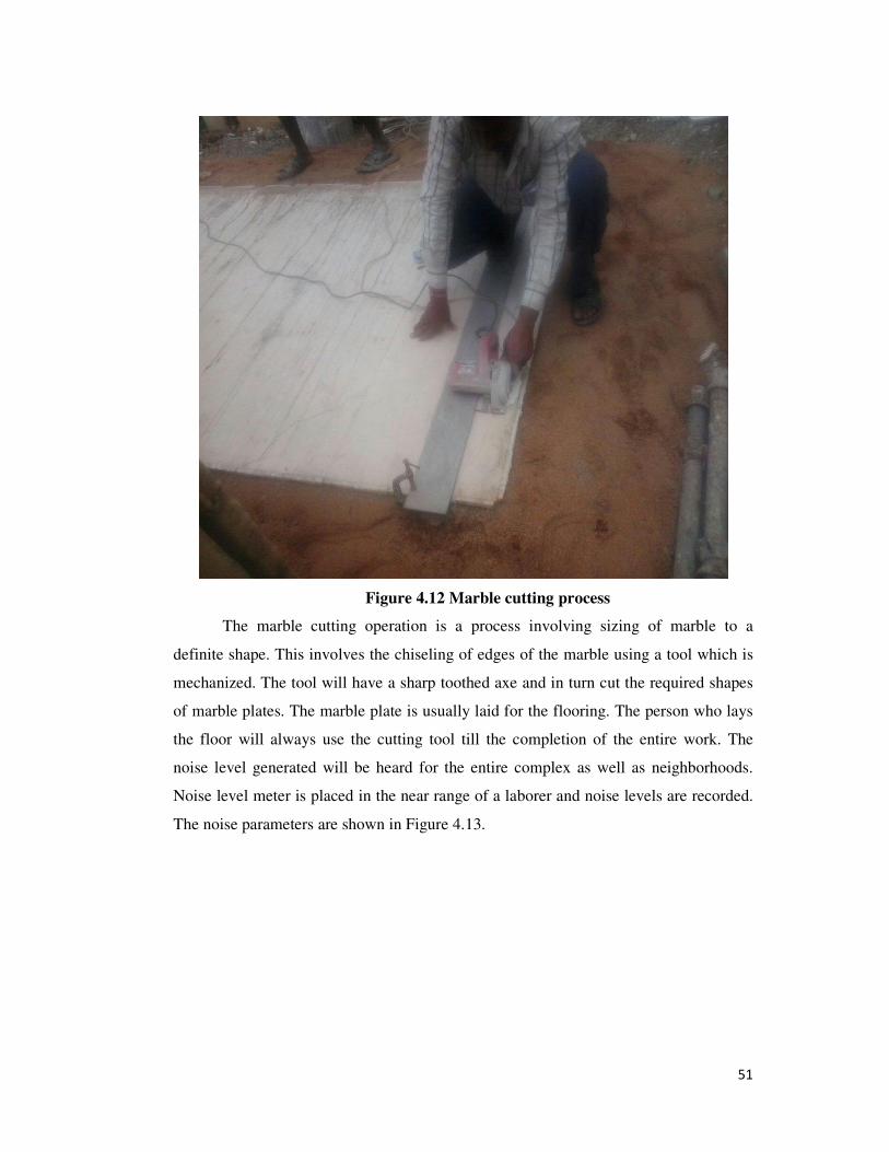
51

Figure 4.12 Marble cutting process

The marble cutting operation is a process involving sizing of marble to a

definite shape. This involves the chiseling of edges of the marble using a tool which is

mechanized. The tool will have a sharp toothed axe and in turn cut the required shapes

of marble plates. The marble plate is usually laid for the flooring. The person who lays

the floor will always use the cutting tool till the completion of the entire work. The

noise level generated will be heard for the entire complex as well as neighborhoods.

Noise level meter is placed in the near range of a laborer and noise levels are recorded.

The noise parameters are shown in Figure 4.13.

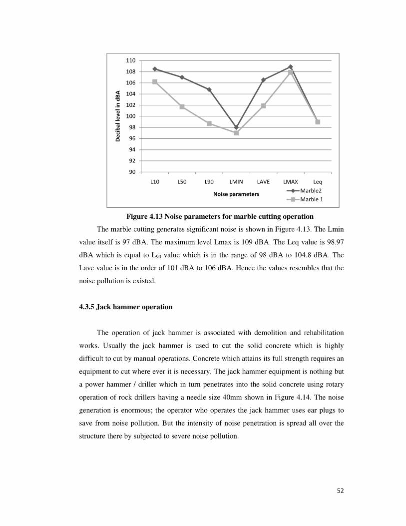
52

Figure 4.13 Noise parameters for marble cutting operation

The marble cutting generates significant noise is shown in Figure 4.13. The Lmin

value itself is 97 dBA. The maximum level Lmax is 109 dBA. The Leq value is 98.97

dBA which is equal to L90 value which is in the range of 98 dBA to 104.8 dBA. The

Lave value is in the order of 101 dBA to 106 dBA. Hence the values resembles that the

noise pollution is existed.

4.3.5 Jack hammer operation

The operation of jack hammer is associated with demolition and rehabilitation

works. Usually the jack hammer is used to cut the solid concrete which is highly

difficult to cut by manual operations. Concrete which attains its full strength requires an

equipment to cut where ever it is necessary. The jack hammer equipment is nothing but

a power hammer / driller which in turn penetrates into the solid concrete using rotary

operation of rock drillers having a needle size 40mm shown in Figure 4.14. The noise

generation is enormous; the operator who operates the jack hammer uses ear plugs to

save from noise pollution. But the intensity of noise penetration is spread all over the

structure there by subjected to severe noise pollution.

90

92

94

96

98

100

102

104

106

108

110

L10 L50 L90 LMIN LAVE LMAX Leq

De

cib

al

lev

el

in d

BA

Noise parametersMarble2

Marble 1

53

Figure 4.14 Jack hammer operation

The present study considered this aspect and the noise level is recorded during the

jack hammer operation for a pile cap work and the duration of recording is for a period

of 6 hours. The noise meter placed at a distance of 4 m radius from the hammer and the

observations were recorded. The noise parameters are shown in Figure 4.15.

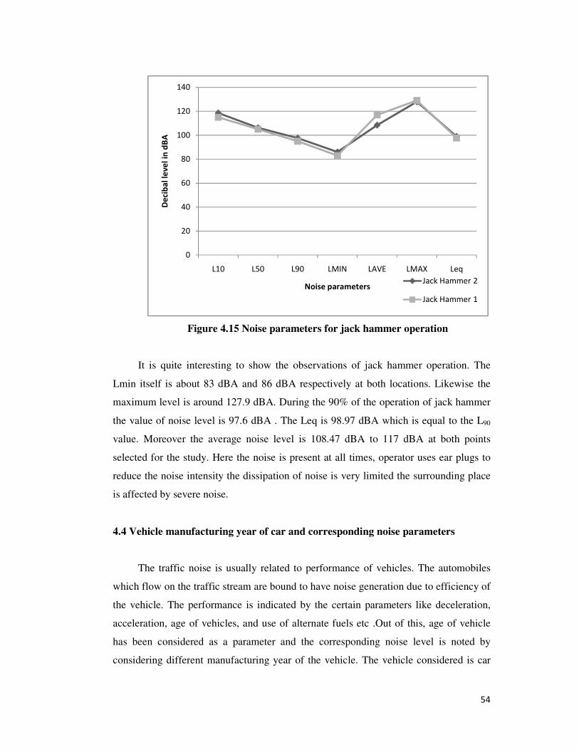
54

Figure 4.15 Noise parameters for jack hammer operation

It is quite interesting to show the observations of jack hammer operation. The

Lmin itself is about 83 dBA and 86 dBA respectively at both locations. Likewise the

maximum level is around 127.9 dBA. During the 90% of the operation of jack hammer

the value of noise level is 97.6 dBA . The Leq is 98.97 dBA which is equal to the L90

value. Moreover the average noise level is 108.47 dBA to 117 dBA at both points

selected for the study. Here the noise is present at all times, operator uses ear plugs to

reduce the noise intensity the dissipation of noise is very limited the surrounding place

is affected by severe noise.

4.4 Vehicle manufacturing year of car and corresponding noise parameters

The traffic noise is usually related to performance of vehicles. The automobiles

which flow on the traffic stream are bound to have noise generation due to efficiency of

the vehicle. The performance is indicated by the certain parameters like deceleration,

acceleration, age of vehicles, and use of alternate fuels etc .Out of this, age of vehicle

has been considered as a parameter and the corresponding noise level is noted by

considering different manufacturing year of the vehicle. The vehicle considered is car

0

20

40

60

80

100

120

140

L10 L50 L90 LMIN LAVE LMAX Leq

De

cib

al

lev

el

in d

BA

Noise parametersJack Hammer 2

Jack Hammer 1

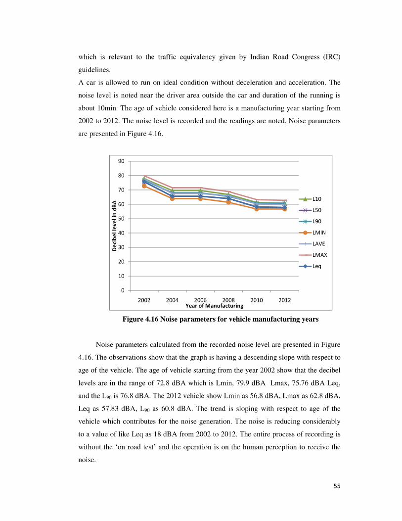
55

which is relevant to the traffic equivalency given by Indian Road Congress (IRC)

guidelines.

A car is allowed to run on ideal condition without deceleration and acceleration. The

noise level is noted near the driver area outside the car and duration of the running is

about 10min. The age of vehicle considered here is a manufacturing year starting from

2002 to 2012. The noise level is recorded and the readings are noted. Noise parameters

are presented in Figure 4.16.

Figure 4.16 Noise parameters for vehicle manufacturing years

Noise parameters calculated from the recorded noise level are presented in Figure

4.16. The observations show that the graph is having a descending slope with respect to

age of the vehicle. The age of vehicle starting from the year 2002 show that the decibel

levels are in the range of 72.8 dBA which is Lmin, 79.9 dBA Lmax, 75.76 dBA Leq,

and the L90 is 76.8 dBA. The 2012 vehicle show Lmin as 56.8 dBA, Lmax as 62.8 dBA,

Leq as 57.83 dBA, L90 as 60.8 dBA. The trend is sloping with respect to age of the

vehicle which contributes for the noise generation. The noise is reducing considerably

to a value of like Leq as 18 dBA from 2002 to 2012. The entire process of recording is

without the ‘on road test’ and the operation is on the human perception to receive the

noise.

0

10

20

30

40

50

60

70

80

90

2002 2004 2006 2008 2010 2012

De

cib

el

lev

el

in d

BA

Year of Manufacturing

L10

L50

L90

LMIN

LAVE

LMAX

Leq

56

4.5 Noise from railway station, level crossing and on road side and the

corresponding noise parameters

Noise from the trains, at railway stations, near level crossing and adjoining roads

is a source of information. Here, a place located at Perungalathur, Tamilnadu, India was

considered. This location is paramount for all south bound movement of traffic from

Chennai. It is a useful link from all sources of national highways across Chennai.

Presently all the south bound intercity buses uses from Chennai, the headquarters of

Tamil Nadu State, uses this place for alighting and boarding passengers who are

transiting from Chennai city to go for down south. Presently the traffic congestion is

severe and another feature is the railway station which is located adjoining to the

national highway. The railway station is bounded by two level crossings one on North

and the other on South. The location of the present study area is shown in Figure 4.17.

The noise level is recorded at three different locations. The locations are railway

station, level crossing and in between track and the national highway. The noise at the

railway station will be exclusively from the trains which are coming from the

neighboring stations. The next location is at the level crossing point and the level

crossing is shown in Figure 4.18.

Figure 4.17 Perungalathur railway station and adjoining places

57

Figure 4.18 Level crossing near Perungalathur railway station

The level crossing is severely trafficked due to movement of vehicles. The

national highway which is adjoining the railway station and track is chosen as the

location for conducting noise survey. Each location is surveyed for two days and each

day for about 8 hours duration. The noise level meter is placed near the railway station

from a distance of about 1 m from the end of the platform. In the level crossing the

noise level meter is placed at a distance of 3 m from the track. On the highway location

it is on the road since there is no designated platform located. The noise level recorded

was calculated for noise parameters and Figure 4.19 shows the observations.

Figure 4.19 Noise parameters for the railway station location

0

20

40

60

80

100

120

Day 1 Day 2 Day 1 Day 2 Day 1 Day 2

Railway

station

Level

crossing

Road side

de

cib

el l

ev

el

in d

BA

Location / Day

L10 L50 L90 LMIN LAVE LMAX Leq

58

The observations made at railway stations and the adjoining places are shown in

Figure 4.19. It shows that railway stations are less prone for noise pollution. The

observation from railway station shows values of Lmin, L90 and L50 are 43.7 dBA,

53.16 dBA and 50.5 dBA, respectively. The noise level of Lmax of 87.4 dBA and L10

of 85.4 dBA are more or less similar and show that the noise generation is marginal.

The cause for the noise exceeding the required level such as 55 dBA mentioned by

CPCB standards is because of air horn ignited from the train. This air horn is for a

period of 10 seconds only and at times only when required. The Leq level is 62.93 dBA

which is the equivalent level with respect to the standards and which is marginally

higher than the standards.

Considering the observations at the level crossing and the road side both are of

similar nature. The representations are shown in Figure 4.19. Figure 4.19 shows that

Lmax level is 107.1 dBA at the Level crossing and 109.1 dBA on the road side. Both

are subjected to vehicular traffic and congested movement. All corresponding values for

both cases, viz., L10 105.1dBA and 104.7 dBA, L50 85.9 dBA and 84.9 dBA,L90 84.81

dBA and 86.4 dBA,Lmin 80.8 dBA and 82.4 dBA, Lave 89.3 dBA and 90.3 dBA,

respectively are calculated and are having similar trend on the vehicular movement to

display noise levels at both the locations. The Perungalathur and adjoining location of

residential zone should have a sound level of 55 dBA. However the noise level

generated is very much on the higher side. The pedestrian movement is 992

persons/hour and this indicates movement of persons and utilization level of the

selected place.

4.6 Flour mills noise during grinding operation

Country like India where people use instant flouring of grains rather packed and

previously powdered grains. The instant flouring operation is carried out in flour mills.

The flour mills are located in the residential areas and the flour mills are having three to

five machines which grind the products for the required smoothness. A flour mill has

been considered here as a source of noise generator and the flour mill is shown in

Figure 4.20.

59

Figure 4.20 Flour mill selected for observation

The flour mills normally consist of grinding machines for rice, mirchi (chilli),

seekakai and spare for maintenance. The flouring operation is carried out whenever

required. The noise generation is enormous and the surrounding place is disturbed with

annoyance in such a way that people are bound to face a lot of health effects. Here, we

consider three flouring operations like rice, mirchi and seekakai as noise generator. The

noise level is recorded for a duration of 2 to 4 minutes during the operation of the

machines. The duration is considered for a set of grinding operation. This operation of

grinding existed for more than 25 to 30 sets in a day of work. The noise meter is placed

at a distance and the noise levels were recorded. The noise parameters are calculated

and shown in Figure 4.21.

Figure 4.21 Noise parameters for flour mills operation

80

85

90

95

100

105

110

RICE FLOUR MIRCHI FLOUR SEEYAKAI FLOUR

De

cib

el

lev

el

in d

BA

Flouring operationL10 L50 L90 Lmin Lavg LMax Leq

60

The flour mill operation is specific in country like India. Here, people mostly use

instant powder mix rather than already powdered mix. The noise generation is more

acute than the other sources. The noise parameters represented in Figure 4.21 show that

the noise pollution existed. The Lmin valve is 89.8 dBA, 90 dBA and 93.8 dBA for the

three flouring operations, respectively. This itself is an indicator for the noise pollution

about the flouring operation. The Lmax is 102.5 dBA, 103.5 dBA and 106.5 dBA,

respectively. All the values of noise parameters are in the range of 92.2 dBA to 106.8

dBA for all the flouring operations. The grinding operation of mirchi is around 3.2 dBA

higher than the other operations. This is because mirchi grinding is operated under

stressful condition, mirchi is in the form of flakes and the fine grain requires extra

power of rotation of machinery. The flour mills are located at the residential localities

and sometimes even in crowded locations. People transiting, utilizing and staying near

the mills are bound to face a lot of hard ships in the form of noise which is significant

from the above test results.

4.7 Findings from observation

It is generally found that people feel much pain in their ears and migraine during

duty hours as well as after duty hours. This study suggests that noise induced hearing

loss is a great challenge in environmental pollution. This noise exposure and

occupational noise exposure both interfere with their activities in their personal life as

well as their healthy living. The findings of this study also indicated the high density

residential area like OMR affected by noise pollution that took a developed residential

area in the vicinity. Indeed some control measures and proper planning has to be

implemented to overcome the adverse effects from noise pollution and for the well

being of the residents.

61

CHAPTER 5

RESULTS AND DISCUSSION

5.1 Analysis of Noise Data

All the observations from the primary survey are presented in each phases and

the results are arrived. Each noise parameters has its own implications but mostly the

noise level like L10, L50, L90, Leq, Lmin, Lmax, Lave were considered for result analysis. The

observations are compared with the standards prescribed by the competent authorities like

MoEF and CPCB (2000).

5.1.1 Results Based on Traffic Noise

The noise parameters calculated from the traffic noise are compared with MoEF

standards and presented in Figure 5.1 for both the locations.

Figure 5.1 Comparison of Leq with CPCB standards for both locations

0

10

20

30

40

50

60

70

80

90

MONDAY TUESDAY WEDNESDAY THURSDAY FRIDAY SATURDAY

De

cib

el

lev

el

in d

BA

Day of Survey TOLL PLAZA SRP TOOLS

CPCB

62

None of the two places recorded below 55 dBA. The values are in the range of

44 dBA and 105 dBA. The highest noise level recorded was during Wednesdays and

Thursdays. The scenario is same at both the sample points. The high level of noise

existed when compared to the standards laid down by CPCB.

The Leq level is alone compared with the CPCB where as if we observe from

the Table 4.1 and Table 4.2 it is clear that L10, L50, L90 values representing the time

duration of noise levels existed. These values show an increase of around 2.7 dBA to

22.7 dBA from standards set by CPCB. The noise level is generated because of

excessive number of vehicles that are plying along the OMR and the noise intensity

heard at surrounding places.

It is high time to evaluate a measure so that the noise intensity can be reduced.

The road way width is two-way and four lane highway, whereas in Chennai this case is

not predominant and the lane width is at times two lanes alone. The road way width is

also limited to and the people are subjected to severity of noise pollution.

In order to furnish the existence of noise pollution across the other states,

observed noise level at OMR areas are compared with other studies carried out in

different parts of India and it was found that, other urban areas also faced the similar

trend of noise pollution (Table 1.1). Thus, there is a need to create awareness among the

people about the rising noise pollution.

To reduce noise pollution, several measures can be implemented such as proper

maintenance of vehicles and roads, plantation of trees and application of appropriate

technology of providing noise barriers and enclosures will go a long way in the

abatement of high level of noise.

5.1.2 Results Based on Vehicular Noise on Pedestrian

The pedestrians are the persons who directly receive the noise pollution from the road

traffic. The road users are subjected to severe noise impact and this is shown in this

research. The noise level Leq is compared with the CPCB standards in the case of

Tambaram subway and is shown in Figure 5.2.

63

Figure 5.2 Noise level compared with CPCB standards

The noise level is higher than the CPCB standards by about 12.66 dBA to 22.67

dBA at both locations. On Saturdays and Sundays the noise levels are higher than the

normal days and show that the traffic is uniform through the week.

o The noise is predominant on all days both inside and outside the subway

o Leq level outside the subway is 72 dBA to 85 dBA and inside is 65 dBA to 80

dBA.

o The pedestrian rate is 700 persons/15 min and the vehicle rate is 1200

vehicle/hour. This rate shows that people suffer due to severity of existing noise

level.

o The location of subway very close to the highway and the subway surrounded

by crowded hawkers making the provision of a noise attenuating measure to

eliminate noise a difficult task.

5.1.3 Results Based on Noise Generated From Machinery (Construction)

Construction noise makers, e.g., heavy earth moving equipment, jack hammer,

marble cutting machine and vibrator machines are taken as examples for this study. The

noise parameters calculated from the primary survey are compared with the standards

set by MoEF and are presented in Figure 5.3.

0

10

20

30

40

50

60

70

80

90

100

Mon Wed Fri Sat Sun Thurs Tues

Out side

Subway

Inside

Subway

de

cib

el

lev

el

in d

BA

Day / Location

Leq

LCPCB

64

Figure 5.3 Noise level compared with CPCB standards

Figure 5.3 shows the simple comparison of Leq level with CPCB standards. The

CPCB standards set for the construction works is shown in Table 1.2. The construction

is multi activity oriented work and it involves different kinds of operation

simultaneously. The standard set by MoEF states that the noise limiting values are 75

dBA for compactors, vibrators, mixer, cranes and saw. Apart from these limits there are

certain rules to be complied for the construction activity like noise level should not be

maintained for more than 5 min interval, acoustic barriers to be provided, provision of

fencing around the sites and temporary earth bund around site using soil. From MoEF

guidelines the observations are now compared and shown that except mixer machine

and vibrator all the others are generating excessive noise. The noise level is 3 dBA

higher on the piling operation, 23.9 dBA on marble cutting and jack hammer operation.

The operation of all these three is for the entire day of work.

• Except the operation of vibrator and mixer all the equipment are above that

standard prescribed by the MoEF.

• The Leq level of MoEF is 75 dBA, where as it is observed the level is increased

from 6% to 58% from the machinery.

• The Lmin, Lmax and Lave levels are quite higher than the standards except in

vibrator equipment.

0.00

20.00

40.00

60.00

80.00

100.00

120.00

Mixer Vibrator Pile Marble Jack

Hammer

De

cib

al

lev

el

in d

BA

Construction activity

Leq

LCPCB

65

• The standards are prescribed for only 5 min of operation, whereas the machinery

operation is spread for a period of 2 to 8 hours depending upon the scale of

work.

• The level of noise for piling is presented in Figure 4.11 shows the intensity of

noise existed with respect to the time.

At present, there is no specific and detailed legislation to control the noise

pollution in construction except the guidelines given for a specific work.

The construction is a multi operational activity which consists of utilization of

different equipments like jack hammer, electrical conduit cutting, earth moving

equipment, and so on. The present construction now going in tech savvy way, it is high

time to evolve a standard for specific equipments. Moreover, the operations like jack

hammer not only disturbs the existing workers but also the surrounding residential areas

are affected when it is operated.

Normally, earplugs and other types of personal protective equipment (PPE) are

used to control a worker’s exposure to noisy equipment and work areas (Sellappan et al

2014). But this is of not much in use because the existing noise control measure is also

very limited to the present need. So, it is high time to evaluate the control measures

available so as to enable the authorities to provide a suitable control measure. The

control suggested by the researcher is based on the observations from his successive

studies done on these aspects.

5.1.4 Results from railway station and near locations

Railway stations are less prone for noise pollution but the level crossing and the

road side locations are subjected to severe noise pollution. Figure 5.4 shows the

intensity of vehicle crossing at Perungalathur railway road crossing.

66

Figure 5.4 Perungalathur station and level crossing location

The railway stations are receiving noise from the air horn alone. The trains

usually move at a speed of 70 to 100 KMPH and dissipate less noise. When the driver

of the train realizes the necessity of application of air horn he in turn presses the button.

Since the Perungalathur railway station and adjoining places prone for movement of

passengers as well as pedestrians frequent application of air horn existed. The Figure

5.5 shows the noise level at the Perungalathur railway station and nearby locations. The

noise level Lmin is around 37.7 dBA and L90 is 47.7 dBA in the railway station

premises. This shows noise is always at minimum level. The maximum noise of 87.4

dBA and the L10 of 85.4 dBA show that the noise is because of air horn alone in the

railway stations.

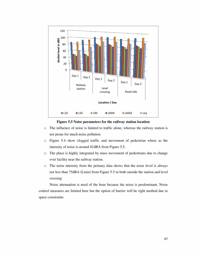
Figure 5.5 Noise parameters for the railway station location

o The influence of noise is limited to traffic alone

not prone for much noise pollution

o Figure 5.4 show clogged traffic and movement of pedestrian where as the

intensity of noise is around 81dBA

o The place is highly integrated by mass movement of pedestrians due to change

over facility near the railway station.

o The noise intensity fro

not less than 75dBA (Lmin) from Figure

crossing

Noise attenuation is need of the hour

control measures are limited here but the option of barrier will be right method due to

space constraints

0

20

40

60

80

100

120

Day 1

Railway

station

de

cib

el

lev

el

in d

BA

L10

oise parameters for the railway station location

The influence of noise is limited to traffic alone, whereas the railway station is

not prone for much noise pollution

show clogged traffic and movement of pedestrian where as the

intensity of noise is around 81dBA from Figure 5.5.

The place is highly integrated by mass movement of pedestrians due to change

over facility near the railway station.

The noise intensity from the primary data shows that the noise level is al

not less than 75dBA (Lmin) from Figure 5.5 in both outside the station and level

Noise attenuation is need of the hour because the noise is predominant. Noise

control measures are limited here but the option of barrier will be right method due to

Day 1Day 2

Day 1Day 2

Day 1Day 2Railway

station Level

crossing Road side

Location / Day

L50 L90 LMIN LMAX Leq

67

oise parameters for the railway station location

whereas the railway station is

show clogged traffic and movement of pedestrian where as the

The place is highly integrated by mass movement of pedestrians due to change

that the noise level is always

in both outside the station and level

the noise is predominant. Noise

control measures are limited here but the option of barrier will be right method due to

68

5.1.5 Results based on year of manufacturing of vehicle (Car)

Car was selected as a parameter for recording observation. The car was allowed

to run without deceleration and acceleration. The relevant noise parameters for this case

are shown in Figure 5.6.

Figure 5.6 Noise parameters for cars

o It is obvious that the vehicle manufacturing and the age of vehicle to run in

traffic stream has significance in contributing to the noise generation.

o Figure 5.6 shows that the noise generation is on down side giving an inference

of deterioration of engine for noise generation

o The Leq level was 78 dBA in the year 2002 and 58 dBA in the year 2012.

o The noise level was measured in an open environment and noise reflection was

marginal

o It is ideal to compare with CPCB standards to show the characteristics of

vehicle during non-operating condition in traffic. However it is generating noise

shown in Figure 5.6.

o Age of vehicle – an important aspect to be analysed for the noise generation.

0

10

20

30

40

50

60

70

80

90

2002 2004 2006 2008 2010 2012

De

cib

el

lev

el

in d

BA

Year of Manufacturing

L10

L50

L90

LMIN

LAVE

LMAX

Leq

LCPCB

69

5.1.6 Results based on flour mills operation

Rice flouring, mirchi flouring, seekakai flouring – these type of flour mills are

predominant in country like India. These types of flour mills are located very near to the

vicinity of residential colony and generate more noise during its grinding operation. The

noises levels are now compared with the standards prescribed by CPCB are presented in

Figure 5.7.

Figure 5.7 Flour mills operation compared with standards of CPCB

The noise levels at the flour mills were excessive as shown in Figure 5.7. The

CPCB has followed the guidelines set by MoEF and was used for comparison. The

flour mills show increase in noise with respect to the standards. All the flour mills are

having Leq level as 93 dBA for rice flour, 96 dBA for mirchi flour and 92 dBA for

seekakai mills operation an increase of about 18 dBA to 21 dBA with respect to the

standards. Of all the flour mills, mirchi flour machine showed more noise pollution. It

showed a 3 dBA increase with respect to other operations. The flour mills operation is a

day to day work and the process carried through all day of week. The flour mills are

located very near to the residential localities and are surrounded by three sides with

walls and front side open. Around 10 sqm of area is provided for the flourmills and the

front side is always open. Since the provision of flour mills are near to the residential

0

20

40

60

80

100

120

RICE FLOUR MIRCHI FLOUR SEEYAKAI FLOUR

De

cib

el

lev

el

in d

BA

Flouring operation

Leq LCPCB

70

colonies and lot of publics will be walking through the roads, it was decided to compare

the level of pollution emitted to a road where human interface existed. The comparison

is shown in Figure 5.8.

Figure 5.8 Comparison between traffic streams with flour mill noise level

To arrive at a meaningful comparison of noise pollution the process identified is

that the people are considered for the effects they face and who are affected directly

because of excessive noise generation. Two sources are identified for comparing noise

pollution one is due to traffic where the pedestrians are facing the hardships and other is

flour mills operation which is situated near the residential localities. The traffic survey

was already done on the OMR road and the noise parameters are calculated and the

observations are already presented in previous chapter 4. Another road indentified for

survey is Kollapakkam-Porur road (KPR) which is running through the residential

localities with less traffic. The comparison and the results are indentified and presented

in Figure 5.8.

o The traffic noise level Leq at OMR was 80.43 dBA which was 46% higher than

the standards set by CPCB of 45 dBA whereas at KRP Leq was 11% higher than

the standards.

0

20

40

60

80

100

120

OMR KPR RICE FLOUR MIRCHI FLOUR SEEYAKAI

FLOUR

De

cib

el

lev

el

in d

BA

Location

L10 L50 L90 Lmin Lavg

LMax Leq LCPCB LMoEF

71

o This was because the volume of traffic at KPR was very less. The noise level

Lmin to Lmax was in the range of 59.30 dBA to 87.90 dBA, at an average

intensity of 75.53 dBA at OMR.

o The corresponding traffic noise level at KPR was 39.90 dBA to 84.30 dBA, at

an average of 47.80 dBA.

o The traffic noise level Lmin at OMR was 59.30 dBA which was well above the

CPCB level of 55 dBA whereas the Lmin at KRP was 39.90dBA which was

well below the standards.

o Noise level L90 - noise level exceeded for 90% of the time in noise recording -

was 66.80 dBA, which was 21% higher than the standards in OMR whereas in

the KPR L90 was 42.20dBA which was well below the standards.

o Noise level high due to the floor mills operation when compared to standards.

o Flour mills are 18dBA to 21dBA higher than the MoEF standards.

o Whereas when compared with CPCB standards on the source specific it shows

that the noise levels in the mills are 38 dBA to 41 dBA more than the standards.

o Both cases of traffic and flour mills are subjected to severe noise intensity. If the

vehicles are less then no noise and the flour mills are not operated then there

will not be any noise.

o The two traffic noise locations show that vehicles contribute to generation of

noise among the humans.

o Both the scenario show that the humans are intervened in both the location but

the only change is noise source.

It is generally found that the people feel much pain in their ears and migraine during

duty hours as well as after duty hours. This study suggests that noise induced hearing

loss is a great challenge to environmental pollution. This noise exposure and

occupational noise exposure both interfere with their activities in the personal life of

people as well as their healthy living. The findings of this study also indicated the high

density residential area like OMR is affected by noise pollution that took a developed

residential area in the vicinity. Indeed some control measures and proper planning has

to be implemented to overcome the adverse effects from noise pollution and for the well

being of the residents.

72

5.2 Solution to noise menace

To tackle this noise menace; a slow poison – A comprehensive study should be

conducted as suggested from this study. With the present government policy and

mechanism in determining the need for mitigation measures to control noise pollution

in the country, an ideal solution is needed. Hence, a noise barrier is an ideal tool to

attenuate the noise which can be put in a place where noise intensity is high and the

surrounding environment is affected. Further study focuses with a suitable barrier

design as a control measure to attenuate noise.

5.3 Noise reduction

It is frequently necessary to use techniques that lower the level of noise on the

road side or at source. A variety of methods are available for noise reduction but they

can be basically grouped as follows: passive and active medium. Active medium differ

from passive mediums in that it is necessary to apply external energy in the noise

reducing process. The absorbing materials, as such, are passive mediums that lower

noise by disseminating energy and turning it into heat given by Environmental

Protection Department Hong Kong (Anon. 2006a).

The techniques employed for noise control can be broadly classified as

• Control at source

• Control in the transmission path

• Using protective equipment.

Out of all the three techniques noise control using transmission path is employed here

to reduce noise against traffic. The control measure is by providing noise barrier in the form

of cubicles and noise reduction is observed.

An attempt has been made to find the noise levels reduction at OMR section; two

sensitive places selected along OMR. It was observed that the noise levels were above

the standards prescribed by the CPCB standards at open stream where as inside barrier

reduction was considerable by about 3% to 20%.

73

5.3.1 Noise barrier

Noise barriers are typically constructed of cast-in-place concrete or masonry block in

certain areas, where space allows and where soil material is available, earth berms are

constructed as noise barriers. The barriers effectively reduce noise levels, but often

cause undesirable secondary impacts, such as blocked views of houses, blocking the

entry point for houses, frontal view, scenic features, and decreased visibility from the

roadway, large shadows cast across a resident’s front yard and backyard for extended

periods of the day. Raising noise barriers to achieve further noise reduction often

exacerbates these secondary impacts (Anon. 2006c). Innovative noise barrier designs

and treatments have been successfully implemented in other countries for a number of

years. These innovative designs have allowed the construction of a noise wall as a

traditional wall. Some of the innovative materials and designs that have been researched

and used in other jurisdictions include transparent panels, semi-translucent concrete

materials, acoustical treatments, and specially designed top treatments, such as curved

or angled tops, irregular top edges, or T-top treatments. Many of these designs have

their own advantages and disadvantages (Anon. 2006c). This research paper deals with

one such barrier: provision along the road side to find the noise levels reduction at

OMR.

The noise barrier selected were

• Noise barrier made of thatched leaves (porous material)

• Noise barrier made of plain cement concrete (non porous material)

• Noise barrier made of fly ash bricks (non porous material)

5.3.2 Barrier made of thatched leaves

A porous plant material called thatched leaves made of coconut leaves was used

as a sound barrier to construct a room on the road side near the sites of measurement.

The sound barrier was installed as a rectangular shed of size 1.5 m × 1.2 m × 2.0 m on

the side of the road as shown in Figure 5.9 and Figure 5.10. Continuous recordings of

Leq measurement during day time was carried out at both study areas. The results showed

that the noise pollution at the places of measurements was wide spread throughout most

74

of its time. The noise in this area was composite in nature consists of transport noise as

well as other sources. After the introduction of the shed there was a considerable reduction

in the level of noise inside the shed. An attempt was made to find the reduction in noise

levels at OMR section; two sensitive places were selected along OMR. It was observed

that the noise levels were above the standards prescribed by the CPCB (Central

Pollution Control Board, New Delhi) at outside the shed whereas inside the shed the

reduction was considerable by about 19%.

Figure 5.9 Thatched leaves noise barrier at Toll Plaza location

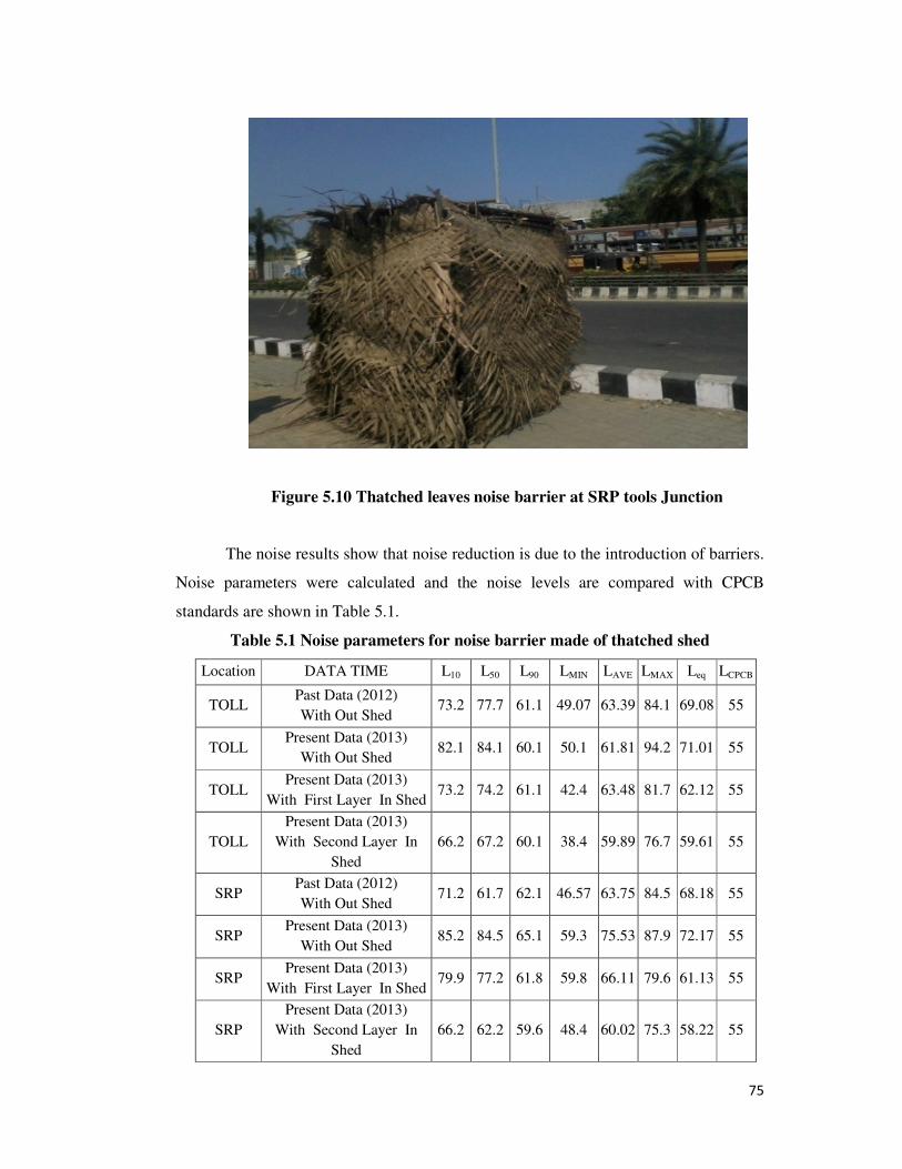
75

Figure 5.10 Thatched leaves noise barrier at SRP tools Junction

The noise results show that noise reduction is due to the introduction of barriers.

Noise parameters were calculated and the noise levels are compared with CPCB

standards are shown in Table 5.1.

Table 5.1 Noise parameters for noise barrier made of thatched shed

Location DATA TIME L10 L50 L90 LMIN LAVE LMAX Leq LCPCB

TOLL Past Data (2012)

With Out Shed 73.2 77.7 61.1 49.07 63.39 84.1 69.08 55

TOLL Present Data (2013)

With Out Shed 82.1 84.1 60.1 50.1 61.81 94.2 71.01 55

TOLL Present Data (2013)

With First Layer In Shed 73.2 74.2 61.1 42.4 63.48 81.7 62.12 55

TOLL

Present Data (2013)

With Second Layer In

Shed

66.2 67.2 60.1 38.4 59.89 76.7 59.61 55

SRP Past Data (2012)

With Out Shed 71.2 61.7 62.1 46.57 63.75 84.5 68.18 55

SRP Present Data (2013)

With Out Shed 85.2 84.5 65.1 59.3 75.53 87.9 72.17 55

SRP Present Data (2013)

With First Layer In Shed 79.9 77.2 61.8 59.8 66.11 79.6 61.13 55

SRP

Present Data (2013)

With Second Layer In

Shed

66.2 62.2 59.6 48.4 60.02 75.3 58.22 55

76

• The observations show that noise reduction is attained because of providing

noise barrier.

• Location of installation of noise barrier is same as the noise recorded in the

traffic stream

• Leq at the time of traffic data recorded was 69.08 dBA at Toll Plaza and 68.18

dBA at SRP location but during the time of observation at installation of barrier

the values are 71.01 dBA 72.17 dBA, respectively.

• The above statement shows that noise level is increasing or not up to the

standards.

• The results of noise level with barrier Leq level is 62.12 dBA and 59.61 dBA at

Toll Plaza location for first layer and second layer of thatched leaves whereas at

SRP location 61.13 dBA and 58.22 dBA, respectively.

• Noise reduction is possible and noise reduction is predominant when two layers

of thatched leaves barriers are provided.

• Noise reduction and the percentage of noise reduction are shown in Table 5.2.

Table 5.2 Details of noise reduction at both locations

Parameter

% Increase of noise

from past (2012) to

present date of

recording (2013)

% of noise

reduction due to

shed consisting of

first layer

% of noise

reduction due to

shed consisting of

second layer

Toll

Plaza

SRP

tools

Toll

Plaza

SRP

tools

Toll

Plaza

SRP

tools

Leq 3 6 13 15 16 19

LMAX 12 4 13 9 19 14

LMIN 2 28 15 0 23 19

LAVE 2 18 3 12 3 21

• The noise Leq is increased from the past data collected in 2012 to present date of

recording in 2013

• The increase in noise level is 3 to 6 % from the past data to present data

77

• The Table 5.2 shows that there is a considerable reduction on providing barrier

• The percentage reduction of noise level ranges from 3 to 10

• The provision of thatched leaves shows that the noise level can be reduced

considerably.

• The selected area is a suitable location because of highly congested place

• The provision of noise barrier as an enclosure found to be a suitable alternative

solution for noise control measure.

• This is suitable for all places, low cost technique not requiring skilled manpower

for installation, flexible in altering the design, can be installed in critical places

where other measures are ineffective.

5.3.3 Noise barrier made of plain cement concrete and coral shell powder concrete

The noise barrier provided was cement concrete blocks made of plain cement,

aggregates and partial replacement of cement with powder made from coral shells with

aggregates. Plain cement concrete were nothing but conventional 100% cement

concrete blocks and Coral Shell Powder (CSP) blocks are cement concrete blocks

where cement is partially replaced by about 10% during concrete mixing. The M30

mix concrete was used for both types of concrete blocks. The blocks are of size 15 cm ×

15 cm × 15 cm. The blocks were stacked as cubicles as shown in Figure 5.11 and

Figure 5.12 at both locations.

The noise barrier was installed as rectangular cubicles of size 0.60 m × 0.60 m ×

0.60 m on the side of the road. Figure 5.11 and Figure 5.12 shows a schematic view of a

noise barrier as concrete cubicles constructed both with conventional concrete and CSP

concrete at the selected locations. Continuous noise level is recorded and duration of

noise recording is presented in previous chapter. Noise level is first recorded in traffic

stream, followed by providing noise barrier in the form of cubicles. Noise meter is then

placed inside the cubicles at both type of concrete blocks noise levels were recorded.

Noise levels recorded were calculated for noise parameters and are presented in Figure

5.13 and Figure 5.14.

78

Figure 5.11 Concrete noise barriers as cubicles at SRP Tools location

Figure 5.12 Concrete noise barriers as cubicle at Toll Plaza location

Figure 5.1

Figure 5.14 N

Noise levels recorded are compared with the CPCB

calculated and are presented in Figure 5.

Results show that there is considerable reduction by the provision of noise barrier

• Noise level leq is 69.08

0

20

40

60

80

100

LMINLAVE

De

cib

el

lev

el

in d

BA

Noise parameter

0

20

40

60

80

100

LMINLAVE

De

cib

el

lev

el

in d

BA

Noise parameter

13 Noise parameter for Toll Plaza location

14 Noise parameter for SRP tools location

Noise levels recorded are compared with the CPCB standards. All noise parameters

calculated and are presented in Figure 5.13 and Figure 5.14.

Results show that there is considerable reduction by the provision of noise barrier

Noise level leq is 69.08 dBA on the year 2012 and it was increased to 73.3

LAVELMAX

Leq

Toll plaza

Noise parameter

Past data (2012) with out

barrier

Present data (2013) with out

barrier

Cubicles made of normal

concrete

Cubicles made of CSP

concrete

LCPCB

LAVELMAX

Leq

SPR Tools

Noise parameter

Past data (2012) with out

barrier

Present data (2013) with out

barrier

Cubicles made of normal

concrete

Cubicles made of CSP

concrete

LCPCB

79

All noise parameters

Results show that there is considerable reduction by the provision of noise barrier

on the year 2012 and it was increased to 73.3 dBA

Past data (2012) with out

Present data (2013) with out

Cubicles made of normal

Cubicles made of CSP

Past data (2012) with out

Present data (2013) with out

Cubicles made of normal

Cubicles made of CSP

80

in 2013 at Toll Plaza location, similar trend is continued in SRP tools location.

• Noise level is 60.5 dBA and 61.1 dBA inside both cubicles at Toll Plaza

location, where as 58.85 dBA and 59.64 dBA at SRP tools location

• Noise level is reduced inside the cubicles and the reduction is shown in Table

5.3.

• Noise level maximum is 86.1 dBA in 2012 and which has been increased to 98.2

dBA in 2013

• Day to day the noise level is increasing, this is due to number of vehicles keeps

on increasing.

• The comparison of CPCB standards also show that noise level is increasing at a

rate of about 18.33 dBA

• Noise pollution is at negligible level inside the cubicle and the levels are slightly

equal to CPCB standards.

Table 5.3 Details of noise reduction at both locations

Reduction of noise level from present data to cubicles made of normal concrete

Reduction of noise level from present data to cubicles made of CSP concrete

All values are in Decibels

Toll Plaza SRP tools Toll Plaza SRP tools

Leq 11.2 11.31 10.8 10.6

• The reduction shown in Table 5.3 shows that noise is reduced by about 106 dBA

to 11.31 dBA by providing noise barrier in the form of cubicles.

• The conventional concrete and CSP concrete shows that barrier can be provided

as pre-cast unit along the road sides.

• Even though the test is carried as a construction of concrete cubicle there is no

significance loss of noise reflection because the concrete is plain cement

concrete.

• The CSP concrete gives noise reduction of 16.64% which is equal to the normal

concrete.

• The concrete shed as a barrier shows that the noise level can be reduced

considerably

81

• The CSP concrete shows equal reduction of noise with respect to normal

concrete

• There will be a considerable reduction in utilising the cement because CSP is

used as partial replacement.

• The cost is reduced when compared to normal concrete.

• The CSP will be an alternate material for cement because now the cost of

cement escalates daily.

• The selected area is a suitable location because of highly congested place

5.3.4 Noise barrier made of fly ash bricks.

The noise barrier provided was constructed with bricks that are made of fly ash.

The blocks were of size 230 mm × 115 mm × 75 mm (which is a standard size of bricks

used in construction industry). The blocks were then placed along road side and stacked

for the required size as mentioned below and constructed as an enclosure. The enclosure

was installed as a square cubicle of size 1.0 m × 1.0 m × 0.60 m on the side of the road

shown in Figure 5.15 and 5.16.

Figure 5.15 View of noise barrier as a cubicle made of fly ash at Toll Plaza location

82

Figure 5.16 View of noise barrier as a cubicle made of fly ash at SRP tools location

For both locations the process of noise reduction is achieved by reducing the

noise along its transmission path. Here, another way of reducing the noise was used by

providing a cubicle form of enclosure made of fly ash bricks. The data collected from

survey is for duration of about an hour and result is presented in chapter 4. Noise levels

were recorded and noise parameters calculated. The noise levels are further compared

with noise levels prescribed by CPCB and presented in Figure 5.17 and Figure 5.18 in

respect of both the locations.

Figure 5.17 Noise parameters at Toll Plaza with and without fly ash cubicles

0

20

40

60

80

100

120

L10 L50 L90 LMIN LAVE LMAX Leq

De

cib

el

lev

el

in

dB

A

Noise parameters

Toll plaza with fly ash shed Toll plaza with out fly ash shed LCPCB

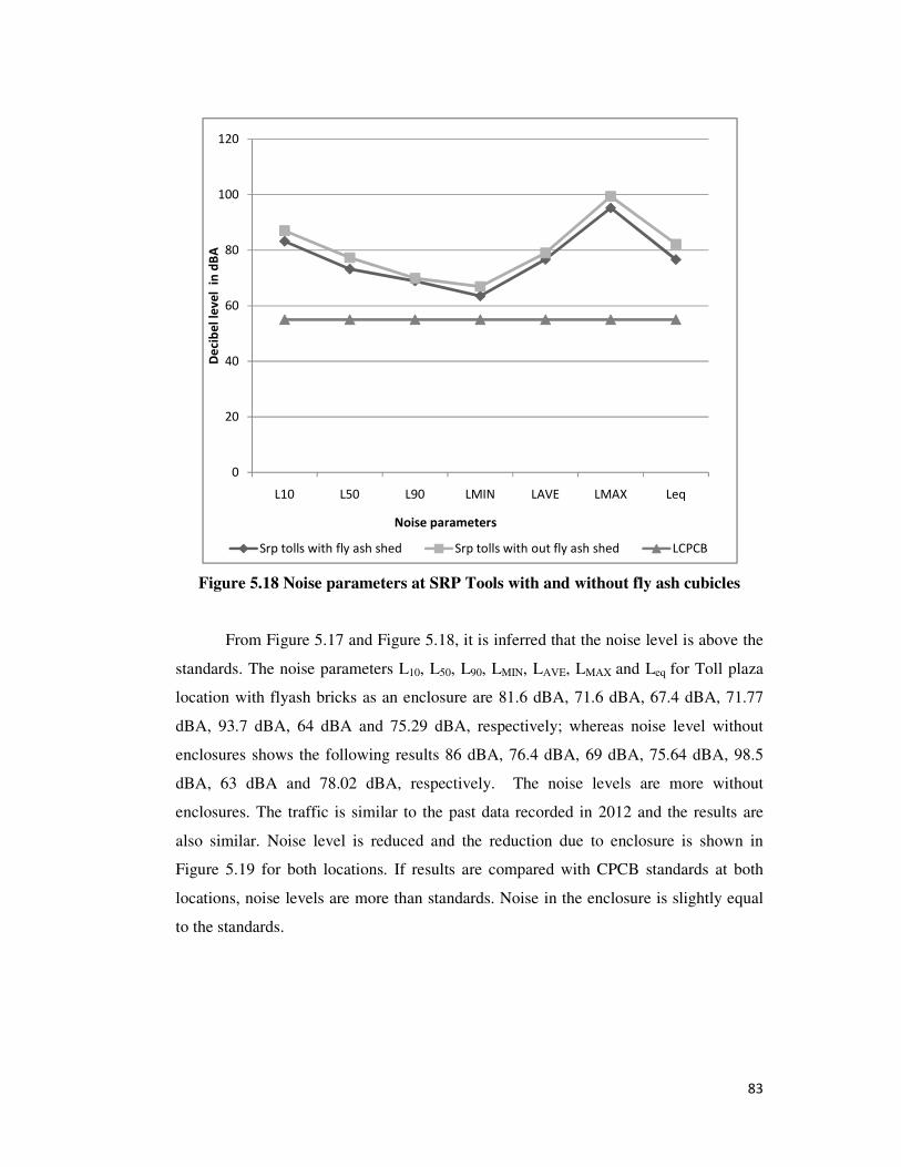
83

Figure 5.18 Noise parameters at SRP Tools with and without fly ash cubicles

From Figure 5.17 and Figure 5.18, it is inferred that the noise level is above the

standards. The noise parameters L10, L50, L90, LMIN, LAVE, LMAX and Leq for Toll plaza

location with flyash bricks as an enclosure are 81.6 dBA, 71.6 dBA, 67.4 dBA, 71.77

dBA, 93.7 dBA, 64 dBA and 75.29 dBA, respectively; whereas noise level without

enclosures shows the following results 86 dBA, 76.4 dBA, 69 dBA, 75.64 dBA, 98.5

dBA, 63 dBA and 78.02 dBA, respectively. The noise levels are more without

enclosures. The traffic is similar to the past data recorded in 2012 and the results are

also similar. Noise level is reduced and the reduction due to enclosure is shown in

Figure 5.19 for both locations. If results are compared with CPCB standards at both

locations, noise levels are more than standards. Noise in the enclosure is slightly equal

to the standards.

0

20

40

60

80

100

120

L10 L50 L90 LMIN LAVE LMAX Leq

De

cib

el

lev

el

in

dB

A

Noise parameters

Srp tolls with fly ash shed Srp tolls with out fly ash shed LCPCB

Figure 5.19

From the results it is shown that there

of barriers. The noise reduction and its percentage are shown in Table

Table 5.4 D

Parameter

Leq

LMAX

LMIN

LAVE

• The result shows that the noise pollution existed.

• Noise levels are at an increasing trend from the year 2012 to year 2014.

• Noise levels are 69.08

dBA in the year 2014. When compared with CPCB levels increment is around

20dBA.

• Even the minimum sound level of 63dB

55dBA.

• This shows that there is an urgent need for controlling the noise pollution.

• Figure 5.19 shows that there is a considerable reduction on providing noise

barrier.

0

10

20

30

40

50

60

70

80

90

Toll plaza

De

cib

el

lev

el

in

dB

A

Past data (2012) with out barrier

With out fly ash cubilces

LCPCB

19 Details of noise reduction at both locations

shown that there is considerable noise reduction by the installation

of barriers. The noise reduction and its percentage are shown in Table 5.4.

Details of Noise Reduction at both locations

arameter % Reduction of Noise from enclosure

Toll plaza SRP tools

5.12 6.77

4.87 4.23

--- ---

3.50 2.79 The result shows that the noise pollution existed.

Noise levels are at an increasing trend from the year 2012 to year 2014.

levels are 69.08 dBA in the year 2012, 73 dBA in the year 2013 and 75.08

year 2014. When compared with CPCB levels increment is around

Even the minimum sound level of 63dBA is higher than the limiting value of

This shows that there is an urgent need for controlling the noise pollution.

shows that there is a considerable reduction on providing noise

Leq Leq

Toll plaza SRP tools

Noise parametersPast data (2012) with out barrier Past data (2013) with out barrier

With out fly ash cubilces With fly ash cubilces

84

considerable noise reduction by the installation

.

Noise levels are at an increasing trend from the year 2012 to year 2014.

2013 and 75.08

year 2014. When compared with CPCB levels increment is around

is higher than the limiting value of

This shows that there is an urgent need for controlling the noise pollution.

shows that there is a considerable reduction on providing noise

Past data (2013) with out barrier

85

• The reduction of pollution inside the barrier comes to about 7% from the

existing road condition

• Even though the reduction is partial but the percentage reduction is significant if

number of vehicles increased.

• Normally, the provision of noise barrier is a cost incurring operation, however,

this type of low cost effective barriers were constructed along highly congested

locations where noise pollution is heavy.

• This is suitable for all locations, low cost technique, not requiring skilled

manpower for installation, flexible in altering the design and can be installed in

critical places where other measures are ineffective.

5.4 Comparison of noise barriers

The barriers effectively reduce noise levels, but often cause undesirable

secondary impacts, such as blocked views of mountains and other scenic features,

decreased visibility from the roadway, or large shadows cast across a resident’s

backyard for extended periods of the day. Raising noise barriers to achieve further noise

reduction often exacerbates these secondary impacts. Following the identification of

available innovative noise barrier designs, a comparison was created to evaluate best

designs. The comparison is shown as table in annexure. Evaluation criteria generally

grouped into performance, material availability, economic considerations,

constructability considerations, maintenance considerations, and aesthetic

considerations. The comparison is shown in Table 5.5.

86

Table 5.5 Comparison of all barriers provided in the study area

Sl.

No.

Comparison

description

Thatched leaves

(1 layer and 2 layers)

Concrete M30 grade

(normal and CSP concrete)

Fly Ash bricks

1 Type of material Porous material Non porous material Non porous material

2 Cost of barrier Low cost barrier High initial cost High when compared to

thatched and low when

compared to concrete

3 Installation Installation is easy It can be pre casted and fixed

3 Suitability Suitable for temporary noise

attenuation

Highly suitable for permanent attenuation

4 Adaptability Due to porous and flexible

adaptability is limited to short

term measure

Meant for long term measure where sure of noise attenuation

5 Aesthetic Aesthetically not ideal but

depending upon usage it can be

installed

Aesthetically ideal and can be a good suitable attenuator

6 Climate

sustainability

The barrier sustainability is

limited to 3 months to 6 months

Permanent barrier only casting and cost involved

7 Environment

friendly

It reduces noise – it is as good

as other material

Waste material like CSP was

used as partial replacement of

cement - utilisation of waste

material has been achieved

Here also we use waste

material like fly ash

8 Percentage of

noise reduction

3% to 10% 11% to 20% 3% to 7%

87

5.5 Noise control barrier

At the present time, the active noise control barrier design is mostly theoretical

and has only seen limited field test installations. There have not been any practical real-

world installations of the active noise control barrier design.

Based on the research and evaluation conducted for this study, it was

recommended that three innovative noise barriers design to be implemented in places

where noise pollution is more than the standards. Barriers are of two different kinds

such as porous and non porous material but have potential to attenuate noise levels. The

barrier which is porous in nature like thatched leaves can be applied as a vertical noise

barrier facing highway traffic. This barrier reduces noise by absorbing noise and

eliminating reflected noise off the face of the barrier. When the traffic is high the noise

levels will also be high in that locations these form of barrier can be installed and the

noise reduction can be attained. In addition during specific requirements like festivals,

special engagements and public meetings these forms of barriers can be erected.

Because these are light in weight, easy to handle, eco friendly and cost effective. The

other form of barrier like concrete blocks, concrete made of CSP blocks and fly ash

bricks blocks which are non porous and has potential to reduce noise by about 15% in

decibel levels can be installed in places where noise source is high like flour mills,

subway, jack hammer, marble cutting places and other noise generating sources.

5.6 Noise prediction

An important factor for the life quality in urban centers like Chennai is related to

the noise levels to which the population is submitted. Several factors interfere with the

amount of noise pollution throughout the city. Among them, and as one of the most

important, is the traffic noise which has been shown in previous chapters. A major

challenge is the quantification of the noise effects on the population. For this reason, to

establish pre- and post-operational measures against such noise problems, noise

prediction simulation is adopted.

88

5.6.1 Noise model necessity

Criteria of road traffic noise in India are based on Leq, therefore any model that

estimates Leq is applicable. As the type of vehicle, noise emission and road structure in

India especially in Chennai is different from other countries. The empirical models such

as FHWA, Stefano, Li, Parida, Gundugdu, Tansatcha and Lam (Golmohammad et al

2007) are not suitable for prediction of road traffic noise in Indian condition. Here, the

mode of transport is from bi cycle , two wheeler, car, share auto, auto, LCV, HCV, Bus

and sometimes bullock carts as per Saxena (1989) and Staff Reporter (2013). In this

thesis a statistical model for predicting -weighted equivalent level is proposed for

Indian condition to design a road traffic noise prediction model from traffic variables.

5.6.2 Contributors for predicting noise

There are more than 10 factors such as volume of vehicles, mode of vehicles,

speed of the vehicles, number of pedestrians, pavement width, surface of pavement,

height of building from road way, observation of noise level from its source, etc.

Golmohammad et al (2009). The list is enormous that contributes to the generation of

noise among the humans. Measuring all the variables for predicting road traffic noise is

difficult and also it is a long term process. Therefore in this research a compact model

with four variables were adopted to obtain a prediction of noise level. The purpose of

this study is to introduce a compact road traffic noise model from traffic variables and

conditions for the city like Chennai. The researcher has suggested the basic parameters

such as volume of vehicles, mode of vehicles, sound source distance from observation

point and speed of vehicles as exploratory factors to predict equivalent sound level.

5.6.3 Study area and data collected

The OMR selected for study purpose the sampling locations were Toll Plaza at

Perungudi and an intersection by name SPR Tools where traffic noise was recorded.

The following data were collected by conducting primary survey.

89

• The noise levels were recorded from morning 10.00 AM to 18.00 PM at an

interval of 10 sec from Monday through Saturday at both locations.

• Total volume of vehicles for the entire period.

• No of vehicle/ hr according to the mode of vehicle such as bus, car, LGV, two

wheeler, share auto and HGV.

• The above details have been taken at a sampling rate of two hours on morning

and afternoon and at peak and non peak hour.

• Speed of the vehicle by way of moving car method at SRP tools.

• Noise measurements were taken at a distance of 0.90 m and 1.10 m from the nearest

road band

• The height of noise measurement is 130cm above the road surface

It was assumed that only these modes of vehicles types contribute to the road traffic

noise and that all vehicles can be categorized into one of these classes. The noise levels

vary within the selected categories due to their variations within the classes and the

condition of the vehicles, mode of operation of vehicles and speed of vehicles.

90

CHAPTER 6

MODELS FOR PREDICTION

6.1 Developing model based on traffic parameters

Using the contributing parameters, the urban traffic noise pollution for the

whole city could be predicted as described below. The method of prediction was to find

out mathematical and physical models that could be applied to real like scenario and for

future development. As the traffic noise pollution was not the same as other types of

pollution, the multiple linear regression method was the best suitable method, since

traffic varied statistically.

The choice of prediction models can be divided into two steps: first to find out

the prediction function and its dependent variable y and independent variable x1, x2, x3

etc., that means to set up a relationship between traffic noise level and some parameters

such as traffic volume, vehicle's type, driving speed, etc; then to establish dependent

variables y. Once the values of y are determined, the prediction can be arrived. The

situations of traffic noise pollution in the future can be predicted using the obtained

regression equation Saxena (1989).

6.2 Regression analysis

Regression analysis is nowadays the most common method employed in traffic

forecasting analysis. The approach is to derive linear equation based on results of the

survey. These relationships are presented in the following forms:

y = a0 + b1x1 + b2x2 + b3x3 + ……….

where, y = dependent variable

a0 , b1, b2 , b3 = Constants (coefficient of regression).

x1 , x2 , x3 = Independent variable

In case of traffic analysis like trip generation it is always the case that variables

are truly independent. For example, vehicle ownership of a house hold is an important

factor for trip generation, but vehicle ownership itself depends on income, household

size, location etc. For structuring regression model, it is necessary to make choice of

91

only those variables which are independent, and have significant effect on end results.

Variables should be continuous in nature, but this is not true always where as zonal

averages make it true.

All of the collected data were entered in the statistical sheet of Excel and SPSS

software. Multiple linear regression models were applied to develop a new model for

Chennai city. The scatter plot of the data would be generated to show if there was any

relationship between Leq and mean vehicles' speed as well as vehicles flow. Therefore,

for the fitted model, the transformation of flow and speed of vehicles were considered.

The developed model and their relationship between them were arrived at and the most

possible R (correlation factor) value was found. The correlation between independent

variable and dependent variable and the cases considered is presented in Table 6.1.

Table 6.1 Variables used and their respective representation

Sl.

No.

Location Case

considered

Dependent

variable

Independent variable

1

Toll Plaza

and

SRP

Tools

C1 – C6

Leq

Type of Vehicles –

Car/LGV/Two-wheeler/Bus/HGV 2

3

C7 – C12 Speed of all type of vehicles

(Car/LGV/Two-

wheeler/Bus/HGV

C 13 Total Vehicles / hour

4 C14 Distance from the source

5 C15 All the above parameters

6.3 Regression Model

The developed model has most possible entrance variable for estimation traffic

noise (Leq). Four groups of independent variables were considered to assist dependent

variable Leq in the model. This designed model can predict Leq at distances of about 0.90 m

to 1.10 m from the roadside edge. Several papers described about modeling of noise

pollution and prediction of noise Leq. The results are shown in Figure 6.1.

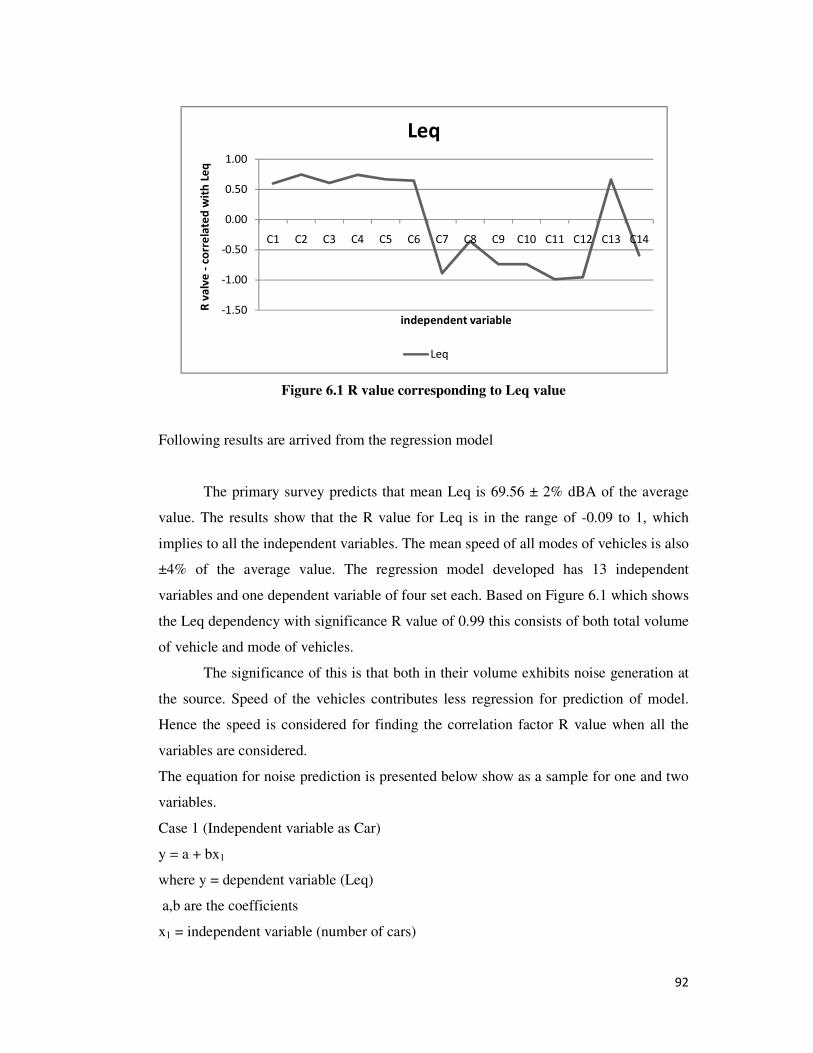
92

Figure 6.1 R value corresponding to Leq value

Following results are arrived from the regression model

The primary survey predicts that mean Leq is 69.56 ± 2% dBA of the average

value. The results show that the R value for Leq is in the range of -0.09 to 1, which

implies to all the independent variables. The mean speed of all modes of vehicles is also

±4% of the average value. The regression model developed has 13 independent

variables and one dependent variable of four set each. Based on Figure 6.1 which shows

the Leq dependency with significance R value of 0.99 this consists of both total volume

of vehicle and mode of vehicles.

The significance of this is that both in their volume exhibits noise generation at

the source. Speed of the vehicles contributes less regression for prediction of model.

Hence the speed is considered for finding the correlation factor R value when all the

variables are considered.

The equation for noise prediction is presented below show as a sample for one and two

variables.

Case 1 (Independent variable as Car)

y = a + bx1

where y = dependent variable (Leq)

a,b are the coefficients

x1 = independent variable (number of cars)

‐1.50

‐1.00

‐0.50

0.00

0.50

1.00

C1 C2 C3 C4 C5 C6 C7 C8 C9 C10 C11 C12 C13 C14

R v

alv

e -

corr

ela

ted

wit

h L

eq

independent variable

Leq

Leq

93

y = 62.49 + 0.0247x1 where R value is 0.596

Similarly if two sets of independent variables are considered (number of cars and speed

of cars)

y = a + b1x1 + b2x2

Where y = dependent variable (Leq)

a,b are the coefficients

x1, x2 = independent variable (number of cars and journey speed of car)

y = -1.3150 + 0.0067x1 + 1.2426x 2 where R value is 0.9362

Likewise for the entire variable can predict the noise Leq value and the R value is

plotted in Figure 6.1.

The predicted and observed value is shown in Figure 6.2 where one can obtain a

residual statistics of about 64.79dbA minimum and 74.45dbA maximum with a

difference of about -1.19dbA to 1.23dbA.

Figure 6.2 Distribution of predicted Leq and measured values

Model suggested by the present researcher is applicable for all condition of road

traffic existed in country like India. Here, pattern of traffic is not uniform and also the mode

of transportation is from public transportation vehicles to private transportation. The share

of private transportation is about 70% of total volume Staff Reporter (2013). The control

measures are limited and the noise is predominant at all the places (Dasarathy and

Thandavamoorthy 2013b).

94

The predicted model is compared with the model study conducted around other

cities and are presented in Table 6.2. There the model is developed based on the certain

independent variables and software for predicting the noise models. The traffic pattern

is complex nowadays and the growth of vehicles is phenomenal. The model with

multiple linear regressions is most common method adopted in traffic analysis. Here,

the consideration is that the independent variable is true to its independence and

continuous in nature (Saxena 1989). For constructing regression models it is necessary

to choose the variables which are contributing to predicting the required noise level

Leq. The present study used a simple method of regression model for predicting traffic

noise level leq. The correlation also has a good range of R value for predicting noise

level.

Table 6.2 Comparison of predicted model with other developed models.

Noise model by

authors

Parameters considered Mathematical

or Software

Mean SD Differenc

e

Measured Leq Mode of Vehicles, total

number of vehicles,

journey speed

Multiple Linear

regression

69.56 3.99

Suggested model

(present study) 69.62 3.49 +0.07

Model by

Golmohammadi et

al (2007)

Mean speed, number of

vehicles in different mode,

distance

Mathematical 69.69 3.45 +0.365

Model by

Golmohammadi

et al (2009)

Mean speed, number of

vehicles, number of trucks,

distance

Mathematical 68.27 3.81 -0.77

Model by

Dan Qun (1989)

Traffic flow, population

near, distance

Mathematical 72.3

±0.10 to -

1.30

Model by

Sooriyaarachchi

et al (2008)

Spot speed, mode of

vehicles, distance

Mathematical

±10.91dBA

Model by

Karantonis et al

(2010)

Total vehicles, mean speed

of vehicles, barriers

provided.etc,

CadnaA and

soundPLAN

75.2 4.8 ±2.3

Model by

Mutairi et al (2009)

Light vehicle ,heavy

vehicle, mean speed of

vehicles number of lanes

US AHWA ±1.0 to 2.0dBA

Model by

Dinesh Kumar

et al (2012)

Growth of vehicles, Lyons Model R2 = 1 to 0.7

95

This study focused on developing a suitable model for noise prediction in

Chennai. The noise prediction models are used as a solution for designing noise

reduction measures and also control measures. Several studies developed regression

models but suitability to the mixed flow of traffic in Chennai is needed now. This

research is the result of noise survey conducted in Chennai in the year 2012, can be

applied to any amount of traffic pattern and has high chance of predicting noise level

with a distance of around 1.0 m from the carriage way.

6.4 Spectral analysis

Noise frequency spectrum influences sound quality especially low frequency

noise (LFN) which gives raise to same level of concern as neighborhood noise and can

have a serious effect on the quality of life of those affected by it. The sources of LFN

may vary from vehicle noise from traffic, wind mills, machinery from industries and

some sensitive equipments. Frequency carries a vital role in detecting sound quality and

propagation. Noise frequency spectrum is taken into account to preciously assess noise

attenuation and mitigation measures

Compared with other environmental noise standards it may initially seem too

stringent to required levels of LFN to be reduced to around the threshold of hearing.

However, there is a growing experience that such low limits are needed to provide

adequate protection from LFN. This is because of the strong reactions and the apparent

difficulty in habituating to LFN (Noise Programme Department of the Environment,

Northern Ireland 2001).

The form of the reference curve has been discussed above. Most existing curves

are based on thresholds of audibility, which have been established for many subjects

over many years, and provides one with the most comprehensive and reliable data about

hearing in the low frequency range. Regarding fluctuations, there is much less data

available. It is not possible to determine the effect of fluctuations through field studies;

for one thing it would not be practicable to survey enough cases, and for another, there

is too much variation between field studies, including the personal situation of the

subjects, the length of exposure and the character of the sound. To establish the effect

96

of fluctuations there is a need to measure the reactions of several people to the same

sound, and this can best be done by setting up tests in the laboratory.

There are limitations in laboratory testing of LFN. In particular, the disturbance

in the field often includes an element of ‘sensitization’ to exposure over extended time,

and this factor cannot be reproduced in the laboratory. Nevertheless, the annoyance of a

sound can be judged by most subjects after a few minutes.

Frequency Composition of Sound is represented in Figure 6.3

Figure 6.3 Frequency distribution

Since the LFN is multiple frequency composition sound, frequency spectrum is

obtained through Fourier Analysis from Brüel & Kjær Sound and Vibration

Measurement A/S (Anon. 2010c).

6.5 Theory about LFN

The LFN problem could occur anywhere in the range 10 –150 Hz but were

usually associated with noise in the 40 – 60 Hz range. The commonest cause of such

noise is industry but there can be many other causes, some of them domestic

(refrigerators, oil fired boilers, and washing machines) and some associated with road

vehicles. Sometimes LFN seems more like vibration than noise and it can cause

structural vibration. It is in any case likely that the business of identifying the source of

LFN will be laborious and may not always be conclusive. LFN is sometimes confused

with vibration. This is mainly due to the fact that certain parts of the human body can

resonate at various low frequencies. For example the chest wall can resonate at

97

frequencies of about 50 to 100 Hz and the head at 20 to 30 Hz (Noise Programme

Department of the Environment, Northern Ireland 2001).

As the A-weighting network attenuates low frequencies by a large amount, any

measurements made of the noise should be with the instrumentation set to linear. For a

preliminary analysis, measurements should be by conducting noise survey and detailed

analysis would need the use of narrower frequency bands or even a FFT (Fast Fourier

Transform) analyses (Can et al 2010).

Spectral analysis was used to determine the frequency composition of sounds.

Spectrum is built by a series of sine waves and Fast Fourier spectral analysis was

carried for the present study. The spectrum analysis is run through MATLAB tool for

each cases and are represented in separate figures.

The procedure adopted for the spectral analysis is each noise source data

recorded through the noise meter is logged. Data which were received from sound level

meter is converted in to signal as an input to the FFT analysis using MATLAB.

6.6 MATLAB

MATLAB is a technical computing environment developed by The MathWorks,

Inc. for computation and data visualization. It is both an interactive system and a

programming language, whose basic data element is an array: scalar, vector, matrix, or

multi-dimensional array. Besides basic array operations, it offers programming features

similar to those of other computing languages, e.g., functions, control flow, etc.

Martinez (2005).

� MATLAB is a program for doing numerical computation. It was originally

designed for solving linear algebra type problems using matrices. Its name is

derived from MATrix Laboratory.

� MATLAB has since been expanded and now has built-in functions for solving

problems requiring data analysis, signal processing, optimization, and several

other types of scientific computations. It also contains functions for 2-D and 3-

D graphics and animation.

98

� Writing User Defined Functions and m-files which can be executed by

specifying some inputs and supply some desired outputs (Christoph 2001).

� The coding language telling procedure to be adopted for the execution of signal

data from the noise meter and FFT process in the MATLAB.

� This coding language is written in command at the beginning of the m-file and

has to be saved as the m-file with a file name and the same as the function name

has to be retrieved for analysis.

A sample coding language is mentioned and it is written with necessary procedure

and options of performing FFT analysis. Commands can be entered interactively at the

command line or saved them in an m-file. So, it is important to know some commands

for file management. Some of the commands shown in Table 6.3 can be used to list,

view, and delete files. Variables created in a session (and not deleted) live in the

MATLAB workspace. It can recall the variable at any time by typing in the variable

name with no punctuation at the end. It is to be noted that MATLAB is case sensitive,

so Temp, temp, and TEMP represent different variables. MATLAB remembers the

commands that one enters in the command history. There is a separate command history

window available via the View menu and certain desktop layouts. One can use this to

re-execute old file with new in formations.

Table 6.3 File Management Commands

Command Usage

dir, less Shows the files in the present directory.

delete filename Deletes filename.

cd, pwd Show the present directory.

cd dir, chdir Changes the directory. There is a pop-up menu on the

toolbar that allows the user to change directory.

type filename Lists the contents of filename

edit filename Brings up filename in the editor.

which filename Displays the path to filename. This can help

determine whether a file is part of the standard

MATLAB package.

what Lists the .m files and .mat files that are in the current

directory.

clc;

clear all;

99

close all;

NNN = 10000;

Fs = 200;

F=1000;

YY2=load('f:\SRP TOOLS\With CSP concrete shed.txt');

YY3=load('f:\SRP TOOLS\With normal concrete shed.txt');

YY4=load('f:\SRP TOOLS\With out shed.txt');

l=length(YY2);

T=0:(l-1);

N=512;

figure;

plot(T,YY2); hold on;

hold off;

title('Noise Signal');

xlabel('Time(s)');

ylabel('magnitude(db)');grid on;

for i=1:N/2

freq(i)=(i/256)*(Fs/2);

end

y=fft(YY2,N);

y=fft(YY3,N);

y=fft(YY4,N);

figure;

plot(freq(1:256),YY2(1:256),freq(1:256),YY3(1:256),freq(1:256),YY4(1:256)); hold

on

title('Noise Signal');

xlabel('Frequency(Hz)');

ylabel('Magnitude(db)');grid on;

figure;

title('Noise Signal');

xlabel('Frequency(Hz)');

ylabel('Magnitude(db)');grid on;

plot(freq(1:256),abs(ifft(1:256))/256,'r');

100

hold off;

If more was known about the effects of noise pollution, however, it would be

possible to know exactly how noise effects the environment, and at that frequencies,

making it possible to enact laws limiting noise pollution specifically and with greater

effect, and to learn how much noise is dangerous to humans and the environment.

6.7 Spectral analysis for traffic stream

The noise frequency is random and sample spectrum analysis (Figure 6.4) shows

that the frequency is of range 20 Hz to 40 Hz with a decibel level of 53 dBA to 74 dBA.

The peak frequency of 85 Hz occurred at a sound intensity of 80 dBA. This show that

usually low frequency noise is also has frequency distribution.

Frequency distribution here is oscillatory representation that shows that noise

levels uniformly penetrate into the atmosphere. Noise spectrum shows that noise levels

lie between 61 dBA to 79 dBA during all range of frequencies this implies that it is like

a band width.

Figure 6.4 Spectrum of open traffic stream at SRP tools location

0 10 20 30 40 50 60 70 80 90 10045

50

55

60

65

70

75

80Noise Signal

Frequency(Hz)

Ma

gn

itu

de

(db

)

Open stream on friday

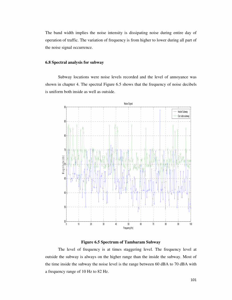
101

The band width implies the noise intensity is dissipating noise during entire day of

operation of traffic. The variation of frequency is from higher to lower during all part of

the noise signal occurrence.

6.8 Spectral analysis for subway

Subway locations were noise levels recorded and the level of annoyance was

shown in chapter 4. The spectral Figure 6.5 shows that the frequency of noise decibels

is uniform both inside as well as outside.

Figure 6.5 Spectrum of Tambaram Subway

The level of frequency is at times staggering level. The frequency level at

outside the subway is always on the higher range than the inside the subway. Most of

the time inside the subway the noise level is the range between 60 dBA to 70 dBA with

a frequency range of 10 Hz to 82 Hz.

0 10 20 30 40 50 60 70 80 90 10050

55

60

65

70

75

80

85

90Noise Signal

Frequency(Hz)

Ma

gn

itu

de

(db

)

Inside Subway

Out side subway

102

Whereas the frequency ranges of 80 Hz to 90 Hz occurs with a decibel level of

75 dBA outside the subway. The maximum decibel level 88 dBA reaches at a frequency

of 77 Hz inside the subway. Outside the subway the maximum decibel level of 84 dBA

reaches on different frequencies. This show that noise frequency is predominant at

outside the subway with a higher decibel level.

6.9 Spectral analysis for construction noise

Construction noise is usually a hindrance to the human interface. Lots of

construction activities require machinery. Noise generation due to machinery nowadays

has become annoyance. The spectral Figure 6.6 shows some light on the frequency

representation of noise levels. Here, noise levels are interpreted for the frequency

representation.

Except the marble cutting operation all other operations falls like a band width

in a frequency range of 0 to 200 Hz with a decibel range of 70 dBA to 80 dBA in the

case of mixer machine and vibrator operation.

Figure 6.6 Spectrum of construction noise

Whereas the decibel range is 90 dBA to 100 dBA for piling work, jack hammer

shows a decibel level of 100 dBA to 120 dBA. The band width form of frequency

0 20 40 60 80 100 120 140 160 180 20060

70

80

90

100

110

120

130Noise Signal

Frequency(Hz)

Ma

gn

itu

de

(db

)

Jack hammer

Pile operation

Marble cutting

Vibrator

Mixer machine

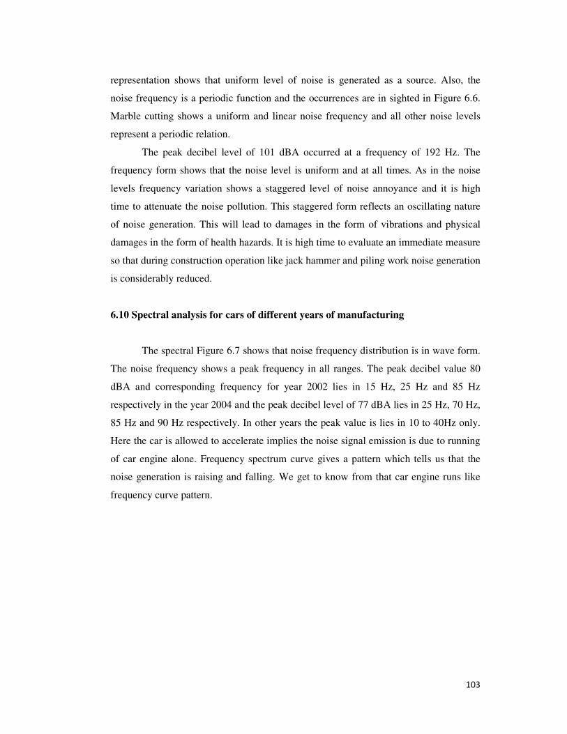
103

representation shows that uniform level of noise is generated as a source. Also, the

noise frequency is a periodic function and the occurrences are in sighted in Figure 6.6.

Marble cutting shows a uniform and linear noise frequency and all other noise levels

represent a periodic relation.

The peak decibel level of 101 dBA occurred at a frequency of 192 Hz. The

frequency form shows that the noise level is uniform and at all times. As in the noise

levels frequency variation shows a staggered level of noise annoyance and it is high

time to attenuate the noise pollution. This staggered form reflects an oscillating nature

of noise generation. This will lead to damages in the form of vibrations and physical

damages in the form of health hazards. It is high time to evaluate an immediate measure

so that during construction operation like jack hammer and piling work noise generation

is considerably reduced.

6.10 Spectral analysis for cars of different years of manufacturing

The spectral Figure 6.7 shows that noise frequency distribution is in wave form.

The noise frequency shows a peak frequency in all ranges. The peak decibel value 80

dBA and corresponding frequency for year 2002 lies in 15 Hz, 25 Hz and 85 Hz

respectively in the year 2004 and the peak decibel level of 77 dBA lies in 25 Hz, 70 Hz,

85 Hz and 90 Hz respectively. In other years the peak value is lies in 10 to 40Hz only.

Here the car is allowed to accelerate implies the noise signal emission is due to running

of car engine alone. Frequency spectrum curve gives a pattern which tells us that the

noise generation is raising and falling. We get to know from that car engine runs like

frequency curve pattern.

104

Figure 6.7 Spectrum of cars manufactured in different years

6.11 Spectral analysis for Perungalathur railway station

The noise frequency curve shown in Figure 6.8 presents a simple comparison

curves. The spectrum is drawn and compared for open traffic, level crossing and

railway station location. The multiple peak frequency occurrences are sighted in all the

curves. The degree of frequency representation is uniform in all cases. For every 10 Hz

of frequency the decibel value is moving from higher range to lower range.

0 10 20 30 40 50 60 70 80 90 10055

60

65

70

75

80Noise Signal

Frequency(Hz)

Ma

gn

itu

de

(db

)

Year 2002

Year 2010

Year 2012

Year 2008

Year 2006

Year 2004

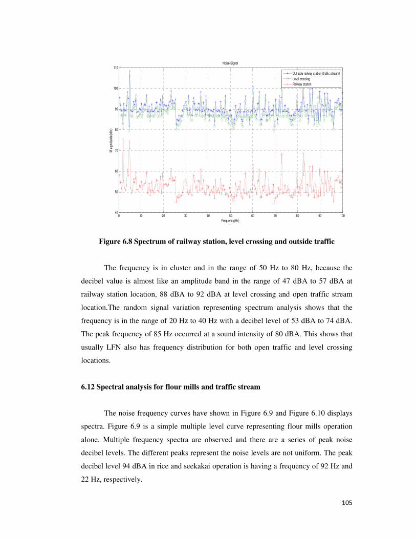
105

Figure 6.8 Spectrum of railway station, level crossing and outside traffic

The frequency is in cluster and in the range of 50 Hz to 80 Hz, because the

decibel value is almost like an amplitude band in the range of 47 dBA to 57 dBA at

railway station location, 88 dBA to 92 dBA at level crossing and open traffic stream

location.The random signal variation representing spectrum analysis shows that the

frequency is in the range of 20 Hz to 40 Hz with a decibel level of 53 dBA to 74 dBA.

The peak frequency of 85 Hz occurred at a sound intensity of 80 dBA. This shows that

usually LFN also has frequency distribution for both open traffic and level crossing

locations.

6.12 Spectral analysis for flour mills and traffic stream

The noise frequency curves have shown in Figure 6.9 and Figure 6.10 displays

spectra. Figure 6.9 is a simple multiple level curve representing flour mills operation

alone. Multiple frequency spectra are observed and there are a series of peak noise

decibel levels. The different peaks represent the noise levels are not uniform. The peak

decibel level 94 dBA in rice and seekakai operation is having a frequency of 92 Hz and

22 Hz, respectively.

0 10 20 30 40 50 60 70 80 90 10040

50

60

70

80

90

100

110Noise Signal

Frequency(Hz)

Ma

gn

itu

de

(db

)

Out side railway station (traffic stream)

Level crossing

Railway station

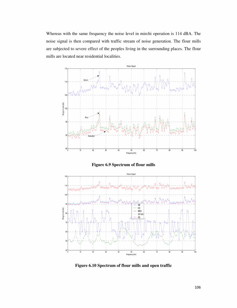
106

Whereas with the same frequency the noise level in mirchi operation is 114 dBA. The

noise signal is then compared with traffic stream of noise generation. The flour mills

are subjected to severe effect of the peoples living in the surrounding places. The flour

mills are located near residential localities.

Figure 6.9 Spectrum of flour mills

Figure 6.10 Spectrum of flour mills and open traffic

0 10 20 30 40 50 60 70 80 90 10085

90

95

100

105

110

115Noise Signal

Frequency(Hz)

Ma

gn

itu

de

(db

)

Mirchi

Rice

Seeyakai

0 10 20 30 40 50 60 70 80 90 10040

50

60

70

80

90

100

110

120Noise Signal

Frequency(Hz)

Ma

gn

itu

de

(db

)

OMR

KPR

MIRCHI

SEEY AKAI

RICE

107

The traffic which is severe along the highway also thrust severe noise impact on

people using the highway. This instance is shown as a spectral frequency curve in

Figure 6.10. For every 10 Hz of frequency the decibel value is moving from higher

range to lower range. The frequency curve is not uniform for the KPR, where as OMR

traffic curve is segmental curve in representing the noise signal level.

The multiple peaks representation of decibel levels corresponding to the

frequency shows vehicles are more in OMR where as it is less in KPR. The peak

decibel level is 69 dBA in KPR and is having 42 Hz as frequency, where as the peak

level of 84 dBA happens in different frequencies. The band width formation of about 10

dBA from 60 dBA to 70 dBA is occurred in OMR traffic stream for a frequency 10 Hz

to 75 Hz.

This shows that the noise level is uniform throughout the time. When compared

to the noise signal from traffic stream the flour mill operation the frequency spectrum is

showing a uniform decibel level. The noise levels are uniform though out the operation

and the peak variance of noise levels are at every frequency intervals.

The human interface is subjected to severity on the uniform rate of noise signal

emission. The frequency represents a non periodic form which is explicit in flourmills

operation than the traffic stream. This is also another indicator for noise levels present

throughout the time of operation. This shows that usually low frequency noise also has

frequency distribution.

6.13 Spectral analysis for noise reduction barriers

The barriers considered are three types, namely thatched shed barrier, normal

concrete cubicle barrier and CSP concrete barrier, and fly ash bricks barrier. The noise

levels recorded allowed consideration for producing frequency distribution as spectrum

analysis. The results are shown in three different Figures 6.11, Figure 6.12, and Figure

6.13, respectively.

108

Figure 6.11 Spectrum of thatched shed to attenuate noise

Figure 6.12 Spectrum of cubicles made of concrete cubes

0 10 20 30 40 50 60 70 80 90 10045

50

55

60

65

70

75

80

85

90Noise Signal

Frequency(Hz)

Ma

gn

itu

de

(db

)

Open stream with out barrier

Tatched leaves as barrier first layer

Tatched leaves as barrier second layer

0 10 20 30 40 50 60 70 80 90 10045

50

55

60

65

70

75

80

85

90Noise Signal

Frequency(Hz)

Ma

gn

itu

de

(db

)

With enclosure (CSP)

With enclosure (normal)

With out enclosure

109

Figure 6.13 Spectrum of cubicles made of fly ash bricks

Noise attenuation can be achieved by different ways of providing a noise control

measure. Here, noise attenuation was achieved by providing a barrier form of noise

control measure. The barrier is made of thatched leaves which are porous material. A

shed was constructed like structure where noise levels are recorded inside the shed.

The thatched leaves were stacked by first layer and second layer, noise levels

were recorded in the case of both layers. The noise levels recorded were compared with

the noise levels recorded at outside the shed to indicate the noise attenuation. The noise

levels recorded were analyzed for spectrum to arrive noise reduction spectrum. Figure

6.11 to Figure 6.13 show spectral analysis and frequency spectrum for all the cases.

While observing the frequency spectrum of the noise signal it is found that there are

multiple peaks around every 10 Hz over the frequency range from 0 to 100 Hz.

The three different frequency spectrums drawn for noise levels show the

following observations. The second layer of thatched leaves shows that lowest noise

level of 48 dBA at a frequency of 75 Hz and 85 Hz. Whereas the frequency of noise

recorded without barrier is 15 Hz for a lowest noise level of 55 dBA. Same way the

0 10 20 30 40 50 60 70 80 90 10040

50

60

70

80

90

100Noise Signal

Frequency(Hz)

Ma

gn

itu

de

(db

)

With fly ash cubicles as barrier

Present data (2013)-open stream

Past data (2012) - open stream

110

peak noise level of 76 dBA for second layer thatched leaves shows a frequency of 21

Hz, frequency of open stream is 75 Hz for the maximum noise level of 88 dBA.

This way the representation of multiple frequency distributions existed for each

frequency value. This staggered form reflects that a noise level is not uniform and at

times peak to its range. In the second layer of thatched leaves shed most of the decibel

values falls between 18 Hz to 82 Hz for a decibel value range of 53 dBA to 61 dBA.

The open stream between the decibel levels of 70 dBA to 80 dBA the frequency 0 to 70

Hz. Cluster of multiple peak show the maximum noise levels existed at all time of

traffic stream in open traffic and also on attenuating barrier. The noise attenuation refers

to noise having different frequency shows noise waves spread through time factors.

Similar way of representation was observed for both the concrete cubicles

shown in Figure 6.12 and for fly ash type of barriers in Figure 6.13. All in the entire

spectrum indicates that noise attenuation is possible by providing barriers. The noise

reducing capability of the barriers is associated with the type as well as its material

properties. Consequently it is presumed that noise reduction associated with frequency

distribution of noise levels existed.

The low frequency noise problems could occur anywhere in the range 10 – 150

Hz but were usually associated with noise in the range of 40 – 60 Hz. The commonest

cause of such noise is industry but there can be many other causes, some of them

domestic (refrigerators, oil-fired boilers, and washing machines) and some associated

with road vehicles.

Sometimes low frequency noise seems more like vibration than noise and it can cause

structural vibration.

It has also been postulated that non-acoustic sources such as high intensity

electromagnetic fields or radar microwaves may create for some people the illusion of

LFN. It will be apparent that LFN presents particular problems for those who have to

deal with complaints about it. It is in any case likely that the business of identifying the

source of LFN will be laborious and may not always be conclusive (Noise Programme

Department of the Environment, Northern Ireland 2001).

111

It is accepted that this problem, though it generates comparatively few

complaints, is a real one. Much remains to be done to extend the understanding of the

nature of LFN and how best to detect and deal with it.

Let the spectrum analysis be catagorized with a simple statement stating the

frequency range with decibel range. The table in Annexure II shows the different

sources of noises, noise levels range and respective frequency in 10 to 40 Hz, 41 to 70

Hz and 71 to 100 Hz.

It is observed that each noise source has its own range of frequency representation.

• The open traffic stream has decibel level of around 51 dBA to 77 dBA around

10 Hz to 100 Hz. This significantly shows that noise levels are predominant at

all times of the survey.

• Tambaram subway shows a different structure when compared to open traffic

stream. The observations are inside the subway and the noise levels are uniform

where it is in the range of 55 dBA to 75 dBA in the respective frequency range.

Whereas outside the subway between 10 Hz to 40 Hz category the noise levels

are 60 dBA – 84 dBA. In the other frequency range the noise levels falls in 69

dBA to 84 dBA. This shows that noise levels are on most of the time higher than

69 dBA.

• Construction operation shows a different range of frequency distribution.

Multiple peak levels show that all activities considered are showing the

maximum to minimum decibel levels in all frequency range. The decibel levels

of jack hammer operation, marble cutting, piling, mixer machine and vibrator

show a peak levels as 127 dBA, 100 dBA, 113 dBA, 97 dBA and 81 dBA

respectively, which are peak levels in all frequency distribution. This shows that

noise levels are not incidental or sudden and the signal presence is always

emitted through each operation of work.

• Four mills generate severe noise effect due to its geographical location. These

mills are operated near the vicinity of people and residential localities. There are

minor variations with respect to maximum value to minimum value in decibel

112

levels. The frequency distribution shows that noise levels are at constant rate

and the dissipation of noise is throughout.

• Barrier provision shows a frequency distribution in a different manner. Multiple

peaks of noise decibel levels are reflected in each category of frequency range

between 41 to 70 Hz. As LFN usually falls in this range, the attenuating barriers

are representing this type of noise levels in the frequency range. Also, open

stream of traffic is severe in all cases of barrier installed places.

The examples show a relationship between the waveform of a signal from noise

levels in the time domain compared to its spectrum in the frequency domain. Most

natural sound signals are complex in shape. The primary result of a frequency analysis

is to show that the signal is composed of a number of discrete frequencies at individual

levels present simultaneously. The number of discrete frequencies displayed is a

function of the accuracy of the frequency analysis which normally can be defined by the

user. This observation together with frequency masking - limitations in the capability of

ears to discriminate closely spaced frequencies at low sound levels in the presence of

higher sounds - is the foundation for the calculation of the loudness of stationary

signals. Loudness of non-stationary signals also needs to take the temporal masking of

the human perception into account.

A suitable experimental analysis for investigating problems in measuring the noise

pollution generated by noise generating sources by using a traditional sound observer

spectrum analysis was presented. Due to the pulsed and noise-like behavior of the

observed signals show LFN existed and serious attenuating measure has to be carried at

the earliest to attenuate noise levels. Most frequency spectra of exterior tyre/road noise

display a prominent peak in the range of 40 to 70 Hz. This research identifies and

examines this peak, analyses its causes and suggests some noise reduction possibilities

through attenuating barriers.

Noise spectra composed of a mix of different sources of noise having a clear

dominance range of 40 to 70 Hz. From this fact, one might be tempted to speculate that

the peak is due to the oscillatory pattern of noise geometry and resulting impact

frequencies. But this could at most be only a partial reason, since the peak frequency

113

relation between different sources of noise generation is the same also for pattern less

type of noise generators.

Having analyzed plenty of data from wave files recorded at selected locations under

different traffic conditions it was observed that the noise power is higher at lower

frequencies in most of the cases and as one goes to higher frequencies, the noise power

rapidly falls down. Later a stage is reached where the noise power is found to be more

or less same with random fluctuations.

6.14 Power Spectrum

Power spectrum estimation can be defined as the method of finding power

values of hidden frequency components in the harmonics of a measured noisy signal,

and is a highly recommended problem in practice. Many applications in engineering

and biomedicine ranging from synthetic aperture radar for image analysis, radar for

determining range of a target, sonar for positioning, speech recognition, heart rate

variability analysis, time series analysis in seismology etc., can be recognized as

spectrum estimation problems. Non parametric power spectrum estimation methods do

not assume any rational functional form but allow the form of estimator to be

determined entirely by the data. Consequently, many methods have been proposed and

developed achieving the spectrum estimation. Some of these methods are called

classical methods and others are called modern methods from national semiconductor

instruments (National 1980).

6.14.1 Power Spectral Density (PSD)

The PSD is the magnitude of the spectrum normalized to a 1 Hz bandwidth.

This measurement approximates what the spectrum would look like if each frequency

component were really a 1 Hz wide piece of the spectrum at each frequency bin. PSD

means when measuring broadband signals (such as noise) amplitude of the spectrum

changes with the frequency span. This is because the line width changes, so the

frequency bins have a different noise bandwidth. The PSD, on the other hand,

normalizes all measurements to a 1 Hz bandwidth, and the noise spectrum becomes

114

independent of the span. This allows measurements with different spans to be

compared. If the noise is Gaussian in nature, the amount of noise amplitude in other

bandwidths may be approximated by scaling the PSD measurement by the square root

of the band width. Thus, the PSD is displayed in units of V/√Hz or dBV/√Hz. Since the

PSD uses the magnitude of the spectrum, the PSD is a real quantity. There is no real or

imaginary part, or phase.

Power Spectral Density (PSD) is the frequency response of a random or periodic signal.

It tells us where the average power is distributed as a function of frequency.

The PSD of a random time signal x(t) can be expressed in one of two ways that are

equivalent to each other

1. The PSD is the average of the Fourier transform magnitude squared, over a large

time interval

====−−−−

−−−−∞∞∞∞→→→→ ∫∫∫∫2

2

2

1dtetx

TEfS ftj

T

TTx

ππππ)(lim)(

2. The PSD is the Fourier transform of the auto-correlation function.

dteRfS

ftjT

Txx

ππππττττ2−−−−

−−−−∫∫∫∫==== )()(

{{{{ }}}})(*)()( ττττττττ ++++==== txtxERx

• The power can be calculated from a random signal over a given band of

frequencies as follows:

1. Total Power in x(t): ∫∫∫∫∞∞∞∞

∞∞∞∞−−−−

======== )()( 0xx RdffSP

2. Power in x(t) in range f1 - f2: ∫∫∫∫ ========

2

112 0

f

fxx RdffSP )()(

The PSD for each signal looks more or less flat across the frequency band.

This type of noise is referred to as white, and if one had taken an infinitesimally small

115

time increment, he/she would see this flatness across the entire frequency band as per

stand for research systems (Stanford 2014).

The reason that there is some variation about the constant level is that one

didn’t take a large enough (i.e., infinite) time sequence of random numbers to calculate

the PSD from. The estimate of the PSD (as calculated in MATLAB) becomes more

accurate as the sample size becomes infinite.

6.14.2 Energy and Power

The total energy in a signal f(t) is equal to the area under the square of the

magnitude of its Fourier transform łF(f)ł2 is typically called the energy density, spectral

density, or power spectral density function and łF(f)ł2 df describes the density of signal

energy contained in the differential frequency band from f to f ± df. In many electrical

engineering applications, the instantaneous signal power is desired and is generally

assumed to be equal to the square of the signal amplitudes i.e., f2(t). Having established

the definitions of this section, energy can now be expressed in terms of power, P(t),

with power being the time rate of change of energy As a final clarifying note, again,

łF(f)ł2 and P(t), as used in equations (1) and (2), are commonly called energy density,

spectral density, or power spectral density functions, PSD. Further, PSD may be

interpreted as the average power associated with a bandwidth of one Hertz centered at f

Hertz.

Here this research estimated the power spectral density of a wide sense

stationary random signal with available low frequency noise signal. The resulting

signals from one after another are processed using MATLAB after the signal data are

processed for FFT analyser. The performance of finding the power spectrum is tested

on different sets of noise signal like traffic stream, flour mills, constructions noise and

barrier type of structures the results are presented in individual cases.

Figures 6.14 to 6.22 show the power spectrum of noise levels recorded for the

different sources. It displays the energy dissipation levels in different forms. Also the

dependence of time is noticed in measuring the noise levels.

116

Figure 6.14 Power spectrum for traffic stream

Figure 6.15 Power spectrum for Kolapakkam Porur Road

0 10 20 30 40 50 60 70 80 90 1002782

2784

2786

2788

2790

2792

2794

2796

2798Spectral density with Random Noise

Frequency (Hz)

Po

we

r in

wa

tt/H

z

traffic at OMR

0 10 20 30 40 50 60 70 80 90 100566

568

570

572

574

576

578Spectral density with Random Noise

Frequency (Hz)

Porur Kolapakkam Road

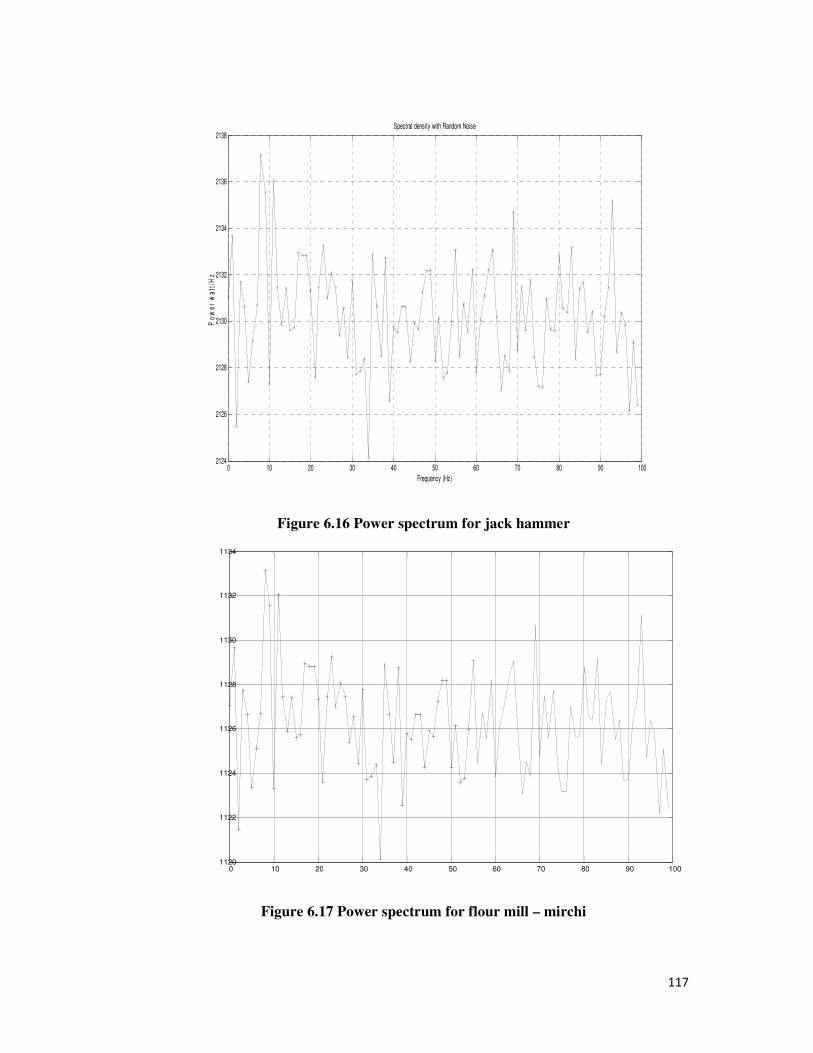
117

0 10 20 30 40 50 60 70 80 90 1001120

1122

1124

1126

1128

1130

1132

1134

Figure 6.16 Power spectrum for jack hammer

Figure 6.17 Power spectrum for flour mill – mirchi

0 10 20 30 40 50 60 70 80 90 1002124

2126

2128

2130

2132

2134

2136

2138Spectral density with Random Noise

Frequency (Hz)

Po

we

r w

att

/Hz

118

0 10 20 30 40 50 60 70 80 901374

1376

1378

1580

1382

1384

1386

1388Spectral density with Random Noise

Frequency (Hz)

Power in watt/Hz

Figure 6.18 Power spectrum for perungalathur level crossing

Figure 6.19 Power spectrum for Perungalathur railway station

0 10 20 30 40 50 60 70 80 90 1001576

1577

1578

1579

1580

1581

1582

1583

1584

1585

119

Figure 6.20 Power spectrum for thatched shed second layer

Figure 6.21 Power spectrum for concrete cubicles

Figure 6.22 Power spectrum for fly ash cubicles

0 10 20 30 40 50 60 70 80 90 100348

350

352

354

356

358

360

362Spectrdom Noise

Frequency (Hz)

pow

er

in w

att

/Hz

Tatched shed second layer

0 10 20 30 40 50 60 70 80 90 100362

364

366

368

370

372

374

Frequency (Hz)

Pow

er

watt

/Hz

fly ash bricks cubicles

0 10 20 30 40 50 60 70 80 90 100319

321

323

325Spectral density with Random

Frequency (Hz)

power watt/Hz

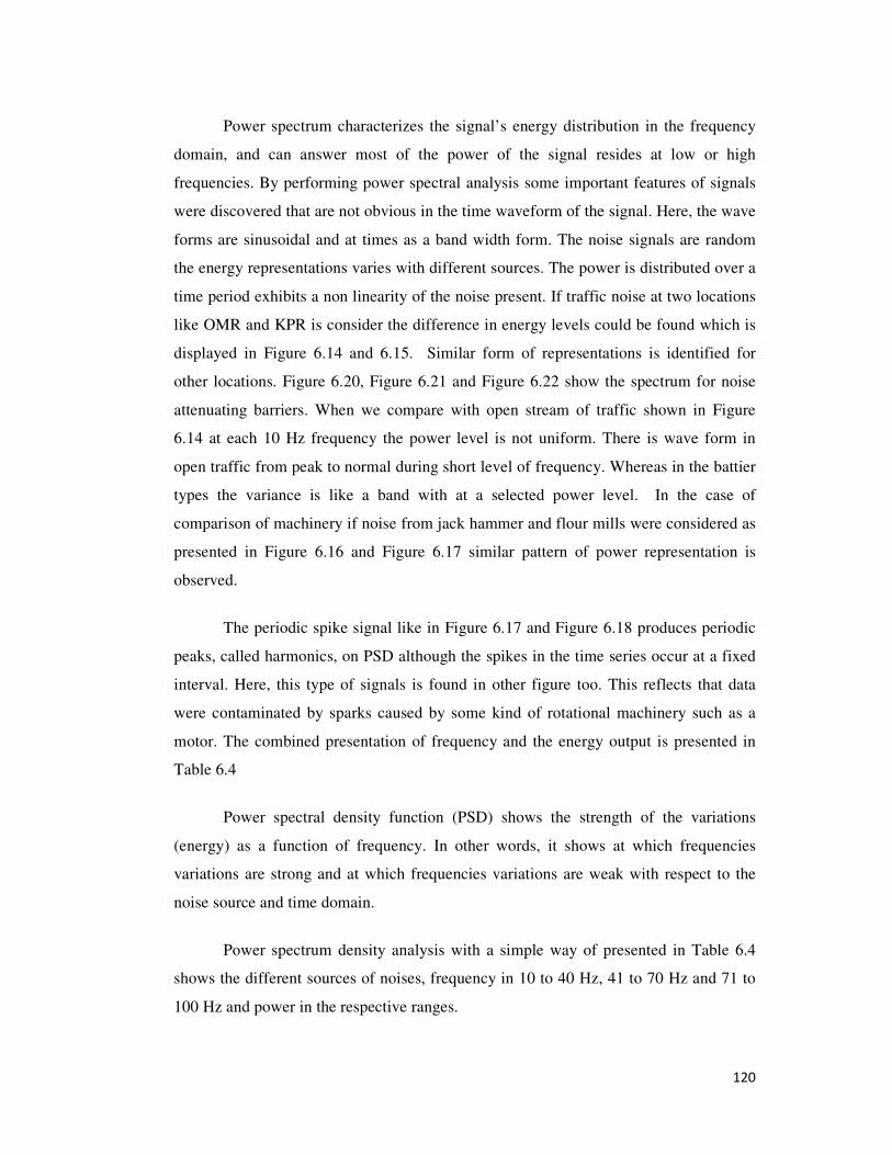
120

Power spectrum characterizes the signal’s energy distribution in the frequency

domain, and can answer most of the power of the signal resides at low or high

frequencies. By performing power spectral analysis some important features of signals

were discovered that are not obvious in the time waveform of the signal. Here, the wave

forms are sinusoidal and at times as a band width form. The noise signals are random

the energy representations varies with different sources. The power is distributed over a

time period exhibits a non linearity of the noise present. If traffic noise at two locations

like OMR and KPR is consider the difference in energy levels could be found which is

displayed in Figure 6.14 and 6.15. Similar form of representations is identified for

other locations. Figure 6.20, Figure 6.21 and Figure 6.22 show the spectrum for noise

attenuating barriers. When we compare with open stream of traffic shown in Figure

6.14 at each 10 Hz frequency the power level is not uniform. There is wave form in

open traffic from peak to normal during short level of frequency. Whereas in the battier

types the variance is like a band with at a selected power level. In the case of

comparison of machinery if noise from jack hammer and flour mills were considered as

presented in Figure 6.16 and Figure 6.17 similar pattern of power representation is

observed.

The periodic spike signal like in Figure 6.17 and Figure 6.18 produces periodic

peaks, called harmonics, on PSD although the spikes in the time series occur at a fixed

interval. Here, this type of signals is found in other figure too. This reflects that data

were contaminated by sparks caused by some kind of rotational machinery such as a

motor. The combined presentation of frequency and the energy output is presented in

Table 6.4

Power spectral density function (PSD) shows the strength of the variations

(energy) as a function of frequency. In other words, it shows at which frequencies

variations are strong and at which frequencies variations are weak with respect to the

noise source and time domain.

Power spectrum density analysis with a simple way of presented in Table 6.4

shows the different sources of noises, frequency in 10 to 40 Hz, 41 to 70 Hz and 71 to

100 Hz and power in the respective ranges.

121

Table 6.4 Frequency range and corresponding energy range

Frequency range in Hz

Location Energy range watts / Hz

10 to 40

Traffic stream

OMR 2792-2785 41 to 70

71 to 100

10 to 40

KPR

569-577

41 to 70 566-576

71 to 100 567-576

10 to 40

Perunglalathur raliway station

and level crossing

Railway station

1376-1381 41 to 70 71 to 100 10 to 40

Level crossing

1577-1584 41 to 70 1577-1582 71 to 100 1577-1582

10 to 100 Flour mill Mirchi 1123-1129

10 to 100 Construction

operation Jack

hammer 2127-2135

10 to 40 Thatched

shed barrier Second layer

353-357 41 to 70 352-358 71 to 100 352-359

10 to 100 Concrete Barrier

cubicles Normal concrete

321-323

10 to 40 Fly ash brick

barrier cubicles Fly ash bricks

352‐357

41 to 70 352‐358

71 to 100 352‐354

It is observed that each noise source has its own range of power spectrum emission.

• The open traffic stream at OMR has decibel level of around 51 dBA to 77 dBA

around 10 Hz to 100 Hz and energy level of around 2792 to 2785 watt/HZ.

Where as in the KPR it is on the 569-576. This show the sound energy emission

is significant level and the volume of vehicles contribute to the excessive level

of difference in frequencies.

• Construction operation of jack hammer and flour mill operation were considered

for power spectrum density and the Table 6.4 shows the following observations.

The noise levels are 93 dBA to 127 dBA for 10 Hz to 200 Hz and energy level

of around 2127 to 2135 Watt/Hz for jack hammer where as for flourmill

operation like mirchi show 105 dBA to 115 dBA, 10 Hz to 100 Hz and 1123 Hz

122

to 1127 Watt/Hz, respectively. The multiple distribution on the power spectrum

figure show that the variance with respect to machinery is more than the

reduction of noise levels.

• Railway station location and the level crossing location show an equal

distribution of energy like 1376 Hz to 1381 Hz and 1571 Watt/Hz to 1583

Watt/Hz, respectively.

• Barrier provision shows a power distribution in a different manner. All the

barriers are of equal power level of 321 Watt/Hz to 357 Watt/Hz. This power is

similar to all frequency range of 10 Hz to 100 Hz.

• Usually low frequency noise does not damage structures. However LFN with

high energy as indicated in Table 6.4 may become detrimental to structures.

Consider the situation, suppose if one is standing on the passenger-loading platform of

the commuter railway line. As the commuter train approaches the station, it gradually

slows down and the train leaves the station it will move in a designated speed. During

this process of slowing down and speeding up the operating engineer sounds the horn at

a constant frequency with a definite pitch he/she will perceive the sound propagation

through waves. The same can be from any source of noise because the signal

transmission through waves to the affected persons. This phenomenon is called Doppler

Effect where source of waves is moving with respect to an observer. Sometimes these

excessive waves create shock wave where the source of waves travelling in high speed.

The distance between the waves goes to zero and so the frequency becomes very high.

More importantly, all of the energy gets concentrated into a very small distance – this is

called a shock wave. In this case, the observer does not hear the approaching source at

all until the shock wave hits with all of the energy in the wave. For sound waves, this

can cause a very loud noise, called a sonic boom. Any time a source exceeds the speed

of the wave, a shock wave will be formed.

Let us consider the following news item in the print media.

A portion of the false ceiling near the first floor check-in counters at the new domestic

terminal of Chennai airport collapsed in the wee hours of Sunday. In the fourth such

incident in the airport in Chennai since last month, a portion of false ceiling collapsed at

the old Anna International terminal on Wednesday. About ten panels of the false ceiling

123

near bay number 28 came crashing down around 3.30 am. However, none was injured

in the incident, airport sources said. A statement from Airport Authority of India said

the slabs measuring 2 feet × 2 feet fell in the international arrival area, which is due for

renovation. “At the time of the incident there was no movement of passengers and the

place was cleaned in an hour,” it said. The airport has been witnessing a spate of

mishaps such as false ceiling falling and glass panels cracking at its new domestic and

international terminals, built at a cost of over Rs. 2,000 crores and raising questions

about the quality of the construction. Since March 31 alone, three incidents of collapse

of granite slabs and glass panels had been reported at the new terminals (Staff Reporter

2014). The above incident reflects a sonic boom is creating in the airport terminal areas

where the excessive sound wave propagates with respect to the noise intensity. Also the

LFN is prevailing due to speeding of aircrafts rather than taking off or landing. The

serious of incident reflects that the incidents are to be addressed. This condition is now

prevailing at the current study where we can say that the noise levels are about more

than 100 dBA to 125 dBA at flourmills and traffic places on OMR. It reveals that here

the LFN about 40 Hz to 60 Hz generates equal amount of energy formation.

This research began looking more closely at the composition of generating sonic booms

including the LFN content. Sound waves influence sonic boom how loud and irritating

it can be perceived by listeners on the ground. Table 6.5 indicates the maximum energy concentration to respective frequency

level for each source of noise. The volume of traffic, noise level at OMR is severe and

noise intensity is about 104 dBA (max level) that shows that the max energy output is

about 2794 Watt/Hz for a frequency of 69 Hz. Correspondingly, the less traffic place

like KPR show a 577 Watt/Hz with a frequency of 40 Hz.

124

Table 6.5 Max energy and corresponding frequency range

Similarly, if noise intensity and the energy output were compared a trend is

observed that if the noise level is lower there is a possibility of energy dissipation on

LFN. This may lead to a source for vibration which includes construction and

excavation equipment, rail and road traffic, and industrial machinery. Low-frequency,

airborne pressure waves are emitted by some heavy vehicles, aircraft and machinery

.This phenomenon can also cause vibration in buildings. Some vibration sources give

rise to audible effects such as structure-borne noise and secondary rattling of building

elements or contents. Yes, high frequency sound waves do possess more energy.

However, that doesn't mean that their vibrations can be felt. Lower frequency sound

waves (at the very bottom of the human hearing range) produce vibrations that can be

felt. The amount of energy in a wave is related to its amplitude. Large-amplitude

earthquakes produce large ground displacements, as seen. Loud sounds have higher

pressure amplitudes and come from larger-amplitude source vibrations than soft sounds.

Max Energy in Watts / Hz

Location Corresponding Frequency in Hz

2794 Traffic stream

OMR 69

577 KPR 40

1583 Perunglalathur railway station and level crossing

Railway station

74

1384 Level crossing

32

1131 Flour mill Mirchi 68

2135 Construction operation

Jack hammer

69

361 Thatched shed barrier

Second layer

32

324 Concrete Barrier cubicles

Normal concrete

68

372 Fly ash brick barrier cubicles

Fly ash bricks

51

125

CHAPTER 7

CONCLUSIONS

From the research carried out in this thesis the following conclusions are drawn.

Knowingly or unknowingly everyone contributes to noise pollution, because

most of the day-to-day activities of human beings generate some noise. Often neglected,

noise pollution adversely affects the human being leading to irritation, loss of

concentration, loss of hearing.

• One has to identify the sources of noise pollution. Once identified, the

reason(s) for increased noise levels are to be assessed.

• It is generally found that the people feel much pain in their ears and

migraine during duty hours as well as after duty hours due to increase in

noise level.

• The findings of this study also indicated that the high density residential

area like OMR is affected by noise pollution.

• Indeed some control measures and proper planning has to be

implemented to overcome the adverse effects from noise pollution and

for the well being of the residents.

• This thesis explores the sources, effects, reactions and suggestions for

controlling the excessive noise generated from road traffic.

• Exposure to noise pollution exceeding 75 decibels for more than eight

hours daily for a long period of time can cause health hazards.

• The traffic noise recorded in open traffic stream at Chennai at two

sensitive places was not below 44 dBA and 105 dBA.

• Survey conducted for different sources of noises show noise pollution

existed. At all sources noise levels are higher than the standards

prescribed by MoEF guidelines.

126

• Pedestrians are severely affected both inside and outside the subway.

Noise decibel levels are 30 dBA more than the MoEF standards. This

reflects how the people who are using road way affected by the severity

of noise

• A comprehensive measure is immediately required and a measure to

attenuate noise is tested and it has proved that noise can be reduced in

Indian condition.

• City like Chennai where construction activities are in brisk phase here

certain operations of machinery show that noise levels are high

• Machinery like jack hammer and marble cutting show a 23 dBA higher

noise levels than standards. There is marginal increase in level due to

piling and running of mixer machine.

• As construction activity is now getting advanced, one needs to consider

different noise standards for different equipments. There are now limited

equipments standards.

• Open traffic stream shows that vehicle contributes less noise levels. The

principle contributor car has been identified as a guide to evaluate noise

levels.

• Different years manufacturing of cars were considered and show that

there is noise level reduction of about 20 dBA from year 2002 to 2012.

This reflects age of the vehicles contribute to noise pollution.

• Railway stations are less prone for noise levels. Noise levels recorded

show a value of 63 dBA even though the station is partly congested one

and passengers are frequently using this station. The nearby area like

level crossing and open traffic show a decibel level of 97 dBA which is

42 dBA more than the standards.

• The need for noise pollution assessment in some flour mills is

demonstrated in this study. The physical measurement reveals that the

noise level status in the three operations of flour machinery is far above

the MoEF guidelines. Thus, the noise pollution level is having impact on

the flour mill employees as well as the public who are residing nearby

the mills and also who uses the mills for flouring.

127

• Flour mills have peoples interference, open traffic are also prone for the

same. The study compared these two aspects and had shown, if less

number of vehicles are operated then noise levels will be considerably

reduced.

• Survey conducted in Kolapakkan-Porur road reflects that noise levels 47

dBA where as OMR noise levels are 80.43 dBA and flourmills show a

noise levels of above 92 dBA.

• There is a need to create awareness among the people and educate the

citizens about the rising noise pollution, health effects, etc.

The excessive noise could cause hearing impairment while this social survey

revealed the level of social and health menace caused by the presence of these mills to

the employees and the people residing in these environments.

The most cost effective measure to reduce noise annoyance is to reduce the

vehicle noise. It has cost measure to reduce noise. Particularly, city like Chennai where

the traffic is more and the use of private transportation becomes higher. The regulatory

measures are minimal and it is high time to focus on alternate measure to reduce noise

pollution. The most suitable non- expensive measure is providing noise barriers.

It has been proved that by providing noise barrier such as thatched leaves, fly

ash brick barriers, noise attenuation of about 3% to 10% was achieved. Where as if

barriers like concrete are provided the noise attenuation can be of about 20%. The noise

barriers are, however, as distinct from façade insulation, also helps to reduce noise in

the outdoor areas.

Presently, this study gives three different noise barriers namely thatched leaves

shed, fly ash (a pollutant) bricks and concrete barrier in form of enclosures. There are

advantages and disadvantages on each barrier nevertheless all attenuate noise to some

extent. Sometimes a severe noise reduction is required, and local measures are the only

alternative.

Such measures are of importance for adapting to local needs like provision of

thatched leaves and sensitive locations where heavier noise recorded may opt for

concrete made of normal concrete or CSP (a pollutant) concrete which will always be of

great importance when helping those exposed to the highest noise levels. CSP concrete

gives equal attenuation that of normal concrete, this proves that low cost barriers are

128

also can be provided. The waste material is recycled to use as a partial binder to get

equal strength that of normal concrete.

The recognition of road traffic noise as one of the main sources of

environmental pollution led to design models that enable one to predict traffic noise

level, to be used as aids for designing roads, change in traffic pattern and highways

planning. In this study a statistical modeling approach has been used for predicting road

traffic noise in Chennai road conditions.

The data sets consisted of more than 3000 measurements on a single day and at

two locations along OMR were considered. The entire data set was utilized to develop a

new model for Chennai traffic condition to predict noise and to be used as a tool for

further prediction. Thus this research suggests the prediction value is ±2% dBA value

accuracy for the developed Leq model.

The individual ear, for the common of people, is not aware at low frequencies.

At low levels of noise, the creature ear attenuates sound by about 25 dB at 100 Hz, 40

dB at 50 Hz and 70 dB at 20 Hz

At upper levels, the effect is not so striking with the attenuation being about 5

dB. This means that frequencies in the region of 20 Hz may not be audible unless the

level exceeds about 70 dB. The A-weighting network found on most sound level meters

is intended to reflect this response.

This study presents LFN for all the noise source considered and an assessment

of urban noise frequency spectrum were drawn using MATLAB software. The results

show multiple peak noise levels variance in every 10 Hz of frequency intervals. Noise

levels were severe and show maximum to minimum in the frequency range of 40 Hz to

70 Hz. Spectra were drawn for all the cases of noise generation.

It has been proposed to estimate PSD for a wide range of stationary random

signals with available low frequency noise. A modified design of algorithm is based on

FFT analysis using MATLAB. The power spectral density simulation results show that

the improved spectral estimation accuracy and shifting of frequency peaks towards the

low frequency region.

The simulation results present a good argument with the published work. In all

cases, the contribution of noise source generated creates waves in the vicinity of the

source. The PSD results obtained indicate that in contrast to high-frequency fields, low-

129

frequency acoustic fields on opposite sides are much more closely connected than

previously believed possible.

Likely practical applications are related to the air–material interface, which occupies

about two-thirds of the surface and are seriously related to each other. The PSD value is

in the range between maximum energy level of 2794 Watts/Hz to a minimum of 324

Watts/Hz. This range spread over all the sources of noise recorded. There is a reduction

of energy in the barriers attenuating energy levels and found to be a value of 324

watts/Hz for a frequency of 51 Hz.

It is clear that LFN a fact of inconsistent transparency can occur where most of

the sound power generated by a source in a noise can be passed into a place. The

results indicate that LFN should not be ignored since there is a possibility of creation of

sonic boom which may be detrimental to the structures. The places where noise survey

was conducted were surrounded by glass facade structures, residential colonies and high

raise buildings with insulating panels, which may conduct acoustic signals through the

air interface. It is high time to evaluate the above to attenuate the noise prorogation

waves by proper mitigation measures.

Noise reduction is the most paramount problem and at any cost this nuisance has

to be reduced. Based on this consideration the thesis addresses the issue of reducing

noise along highway to suite Indian working condition. Here, investigation was carried

out by providing a noise barrier in the form of enclosure.

Knowledge gained from this research

From the study the researcher learned the presence of noise pollution in the

traffic, construction sites, flour mills, etc., and its seriousness. It needs to attenuate

noise by way of providing barriers. Further the researcher learned the effectiveness of

barriers. There are advantages and disadvantages using barrier, there are indirect

benefits of using cost effective barriers like thatched leaves. Also effective use of waste

products like CSP and fly ash show the energy dissipation is marginal in generation of

pollution. This study also tackles the twin problems of noise pollution and

environmental degradation that are created by wastes.

130

REFERENCES

Agbalagba, EO, Akpata, AKO, & Olali, SA 2013 'Investigation of Noise Pollution

Levels of Four Selected Sawmill Factories in Delta State, Nigeria' Advances in Applied

Acoustics (AIAAS), vol.2, issue 3, pp. 83-90

Al-Mutairi, N, Al-Rukaibi, F & Koushki, P 2009 'Measurements and Model Calibration

of Urban Traffic Noise Pollution' American Journal of Environmental Sciences, vol. 5,

no-5, pp. 613-617

Andy Moorhouse, David Waddington & Mags Adams 2005 ' Proposed criteria for the

assessment of low frequency noise disturbance Prepared for Defra' Acoustics Research

Centre, Salford University Project report

Avinash Chauhan & Krishnakumar Pande 2010 'Study of noise levels in different

Zones of Dehradun City', Journal of report and opinion, vol.2, issue-7, pp. 65-68

Balashanmugam, P, Ramanathan, AR, Nehrukumar, V, Balasubramaniyan, V 2013

'Assessment of Noise Pollution in Chidambaram Town', International Journal of

Research in Engineering and Technology, vol. 2, issue. 10, pp. 85 -93

Can, A, Leclercq, L, Lelong, J & Botteldooren, D 2010 'Traffic noise spectrum

analysis: dynamic modelling vs. Experimental observations' Journal of applied

acoustics, vol.71, issue 8, pp. 7645-770

Carvalhoa, APO & Oliveirab, PD, S 2010 'Model of a Benefit/cost Ratio Analysis for

Comparison of Environmental Noise Barriers' Proceedings of NOISE CON 2010,

Baltimore, Maryland, Laboratory of Acoustics, FEUP - Faculty of Engineering

University of Porto, 4200-465 Porto, Portugal

Choudri, VP., Deepak and Ramesh, C., 2011, 'Assesment and control of sawmill

noise,' Proc. International Conference on Chemical and Biological Environmental

Sciences, Bangkok pp 299-303

Christoph Rauscher 2001 'Fundamentals of Spectrum Analysis' Rohde & Schwarz

GmbH & Co. Press, KG Germany edition, Germany

Colin, H, Hansen, Berenice, I & Goelzer, F 2010 'Engineering noise control' World

Health Organization, University of Adelaide, South Australia 5005,

AUSTRALIA,Chapter10 pp. 1-52

Dasarathy, AK & Thandavamoorthy, TS 2013a 'Noise Pollution in Chennai - A Case

Study', Asia Pacific Journal of Research, vol. 1, issue. XI, pp. 143-148

131

Dasarathy, AK & Thandavamoorthy, TS 2013b 'Attenuation of noise using barrier in

the form of enclosures', Journal of Applied Research, vol. 3, issue. 8, pp. 83-89

Datta, JK, Sadhu, S, Gupta, S, Saha, R, Mondal, NK & Mukhopadhyay, B 2006 'Noise

pollution in Burdwan town & its impact', Journal of Environmental Biology, vol. 27,

pp.609-612

Dinesh Kumar, R, Mathivanan, V, Ponmaran, P & Pradeepraj, V 2012 'A Case Study of

Traffic Noise in and around Melmaruvathur', A Project Report, Anna University

Elancheliyan Sellappan & Krishnakumar Janakiraman 2014 'Environmental noise from

construction site power systems and its mitigation', Journal of Noise & Vibration

Worldwide, pp. 14 to 22

Fan Dan-Qun, Liu Ke & Chen Qian 1989 'Prediction and Evaluation of Pollution of

Urban Traffic Noise in China', Science in China Series A, vol. 32, No. 1, pp. 93-100

Fernando, A, N & Castro Pinto 2010 'Urban Noise Pollution Assessment Techniques,

Methods and Techniques in Urban Engineering', Armando Carlos de Pina Filho and

Aloisio Carlos de Pina (Ed.), 96-4, InTech, available from:http://www.intechopen.com

/books/methods-and-techniques-in- urban engineering / urban-noise-pollution-

assessment- techniques

Gilchrist, A, Allouche, EN & Cowan, N 2003 'Prediction and mitigation of construction

noise in an urban environment', Canadian Journal of Civil Engineering, vol. 30, pp.

659–672

Golmohammadi, R, Abbaspour, M, Nassiri, P & and Mahjub, H 2007 'Road Traffic

Noise Model', Journal of Environmental Health Science and Engineering, vol. 7, No. 1,

pp. 13-17

Golmohammadi, R, Abbaspour, M, Nassiri, P & and Mahjub, H 2009 'A Compact

Model For Predicting Road Traffic Noise', Journal of Environmental Health Science

and Engineering, vol. 6, No. 3, pp. 181-186

Heng Li, Zhen Chen, Conrad TC, Wong & Peter, E, D, Love 2000 'A quantitative

approach to construction pollution control based on resource levelling', Journal of

Construction Engineering and Management. ASCE, vol. 126(4), pp. 320-324

Ingunn Milford, Sigve, J, Aasebo & Kjell Strommer 2012 'Value of money in road

traffic noise abatement' Procedia Social and Behavioral Sciences, online on

www.sciencedirect.com.

132

Jadaan, K, Al-Dakhlallah, A (Tomah), Goussous, J & Gammoh, H 2013 'Evaluation

and Mitigation of Road Traffic Noise in Amman, Jordan', Journal of Traffic and

Logistics Engineering, vol. 1, no. 1, pp. 51-53

Ken Kaneuchi & Koichi Nishimura 2011 'Noise Prediction Simulation And Noise

Reduction Technology At Low-Frequencies' Proceedings of International Gas Union

Research Conference, Japan, pp. 1-12

Khursheed Ahmed Wani & Jaiswal, YK 2010 'Assessment of noise Pollution in

Gwalior M.P., India', Journal of Advances in Bio Research, vol. 1, pp. 54-60

Mangalekar, SB, Jadhav, AS & Raut, PD 2012 'Study of Noise Pollution in Kolhapur

City, Maharashtra, India', Universal Journal of Environmental Research and

Technology, vol. 2, issue. 1, pp. 65-69

Marcos, D, Fernandez, Samuel Quintana, Jose A. Ballesteros & Noelia Chavarria 2010

'Are workers in the construction sector overexposed to noise', Journal of Noise &

Vibration Worldwide, pp. 11-15

Mohammad Hassan Ehrampoush, Gholam Hossein Halwani, Abolfazl Barkhordarl &

Mohsen Zare 2012 'Noise pollution in urban environments a study in YAZD city',

Pollution Journal of Environmental Studies, vol. 21, pp. 1015-1100

NarendraSingh & Davar,S,C 2004 'Noise Pollution – Sources, Effects and Control',

Journal of Human Ecology, vol. 6, issue. 3, pp. 181-187

Peter Karantonis, Tracy Gowen & Mathew Simon 2010 'Further Comparison of Traffic

Noise Predictions Using the CadnaA and SoundPLAN Noise Prediction Models',

Proceedings of 20th International Congress on Acoustics, ICA 2010, Sydney, pp. 23-27

Pratapkumar Padhy & Bijaya Kumar Padhi 2006 'Assessments of noise quality in

Bolpur and Santiniketan areas -India', Journal of Environmental Research and

Development, vol. 3, no. 1, pp. 301-306

Qais Banihani & Khair Jadaan 2012 'Assessment of Road Traffic Noise Pollution at

Selected Sites in Amman, Jordan: Magnitude, Control and Impact on the Community',

Jordan Journal of Civil Engineering, vol. 6, no. 2, pp. 267-278

Sagartzazua, X, Hervellab, L & Pagaldaya, JM 2012 'Review in Sound Absorbing

Materials', Arrasate-Mondragón Spain Inc. Publications, Spain

Sanjeeb Mohapathra, Mrityunjay Basankopp & Shrihari, S 2012 'Public Reception And

Response To Traffic Noise Induced Annoyance: A Case Study At Mangalore, India',

Nitk Research Bulletin, vol. 21, no. 2, pp. 39-50

133

Saxena, SC 1989 'A Course in Traffic Planning and Design', first edn. V, Nemichand

and Bros., Roorkee

Sooriyaarachchi, RT & Sonnadara, DUJ 2008 'Modelling Free Flowing Vehicular

Traffic Noise', Journal of Institution of Engineers, vol. 40, no. 2, pp. 43-47

Sumiani Yusoff 1997 'Study on Characteristics of Transportation Noise Sources in

Klang Valley, Malaysia', Journal of Eastern Asia Society Transportation s, vol. 2, no.6,

pp.2053-2069

Tandel, BN & Macwan, JEM 2013 'Assessment And Modeling Of Urban Traffic

Noise At Major Arterial Roads Of Surat, India', Journal of Environmental Research

And Development, vol. 7, no. 4A, pp. 1703-1709

Thangadurai, N, Venkateswaran, P & Jeevanraj, S 2005 'Evaluation and analysis of

noise quality of Ambur, TamilNadu, India' Journal of Environmental Sci and Engg,

vol. 47, pp. 7-12

Tirtharaj Sen, Pijush Kanti Bhattacharjee, Debamalya Banerjee & Bijan Sarkar, 2010

'Study and Comparison of the Noise Dose on Workers in a Small Scale Industry in

West Bengal, India', International Journal of Environmental Science and Development,

vol.1, no. 4, pp. 364 – 370

Turgut Öztürk, Zübeyde ÖZTÜRK & Metehan ÇALIS 2012 'A case study on acoustic

performance and Construction costs of noise barriers', Scientific Research and Essays,

vol. 7, issue. 50, pp. 4213-4229

Vahideh Abolhasannejad, Mohammad Reza Monazzam & Narjes Moasheri 2013

'Comparison of Noise Sensitivity and Annoyance Among the Residents of Birjand Old

and New Urban Districts', Current World Environment, vol. 8(1), pp. 29-36

Vidyasagar, T & Rao, GN 2006 'Noise Pollution Levels in Visakhapatnam City

(India)', Journal of Environmental Science and Engineering, vol. 48, no. 2, pp. 139-142

Wendy, L, Martinez & Angel R. Martinez 2005 'Exploratory Data Analysis with

MATLAB' Chapman & Hall/CRC Press, London SW15 2NU

Yang Fan, Bao Zhiyi, Zhu Zhujun & Liu Jiani 2010 'The investigation of noise

attenuation by plants and corresponding noise reduction', Journal of Environmental

Health, vol. 72, pp.8-12

134

Web reference

Annual Report 2005-2006 to combat noise pollution Activities of the West Bengal

Pollution Control Board (WBPCB), www.wbpcb.gov.in/html/ annualreps/ar0607/

part1.pdf

Anon. 2012 'Report on Noise and Vibrations' Indian Institute of Technology – Roorkee a

ppt presentation.http://www.iitro.in/publications/ppt presentations/html

Anon. 2000 'Transit noise and vibrations assessment' Inc. Publications United States,

chapter 12, pp. 12-1 to 12-12, www.fta.dot.gov/documents/FTA_Noise_and_Vibration

Manual.pdf

Anon. 2000 'The Ambient Air Quality Noise Standards in Respect of Noise as per GOI,

MoEF Notification Environment (Protection) Act 1986 as amended in 2000' CPCB

Chennai, www.envfor.nic.in/legis/noise/noise.html

Anon. 2001 'Environmental health criteria of noise' World Health Organisation, (WHO)

Occupational and community noise, Fact sheet 258, Geneva, www.who.int/quantifying_

ehimpacts/publications/en/ebd9.pdf

Anon. 2006a 'Plan to tackle road traffic noise in Hong Kong' A Draft Comprehensive Plan

Prepared by Environmental Protection Department, Hong Kong, www.epd.gov.hk/epd/

english/environmentinhk/noise/.../LNRS-final.pdf

Anon. 2006b 'Mitigation measures against road traffic noise in selected places' Prepared

by Jackie WU Research and Library Services Division Legislative Council Secretariat,

Hong Kong, www.epd.gov.hk/epd/english/environmentinhk/noise/.../LNRS-final.pdf

Anon. 2006c 'Evaluation of benefits and opportunities for innovative noise barrier design'

A Comprehensive plan prepared by Arizona Department of Transportation [ADOT].

Anon. 2010a 'Understanding the most common sources of noise in the city' New York City

Department of Environmental Protection Bureau of Environmental Compliance 59-17

Junction Blvd, 11th Fl, Flushing, NY, www.nyc.gov/html/dep/pdf/noise_code_guide.pdf

Anon. 2010b 'Good Practice Guide on Noise Exposure and Potential Health Effects'

European Environment Agency – 36, pp ISBN 978-92-9213-140-1 doi:10.2800/54080

Anon. 2010c 'A basic frequency analysis of sound' lecture notes issued by Brüel & Kjær

Sound and Vibration Measurement A/S www.bksv.com/

Anon. 2013 'Noise Pollution and its Control' BITS, Pilani http://discovery.bitspilani.ac.in/

dlpd/courses/coursecontent/coursematerial %5Cetzc362%5C noice_pollution_notes.pdf

135

Controlling noise on construction sites as a BP guide' Australian Construction Agency,

Australia 2007, pp. 1 to 19, www.safeworkaustralia.gov.au/ sites/.../Occupational_ Noise

Environmental criteria for road traffic noise Published by, Environment Protection

Authority 1999, www.epa.nsw.gov.au/resources/noise/2011236nswroadnoisepolicy.pdf

IOMA’s safety director’s report on ' noise hazards at construction sites: there are answers'

Institute of management and administration 2001 pp. 1-3, lib.imps.ac.ir/pdfTemp/

9780123820129.pdf

National Semiconductor Application Note 255, 1980 Japan pp. 1 to 27,

www.ti.com/lit/an /snoa719/snoa719.pdf

Report on Low Frequency Noise Technical Research Support for DEFRA Noise

Programme Department of the Environment, Northern Ireland Scottish Executive

National Assembly for Wales 2001, nf-hrup.si/pdf_files/LFN_scotland.pdf

Report on the Status of Rubberized Asphalt Traffic Noise Reduction in Sacramento

County Prepared by: Sacramento County Department of Environmental Review and

Assessment, Inc. Consultants in Acoustics and Noise Control Engineering 1999,

http://www.ra-foundation.org/report-on-the-status-of-rubberized-asphalt-traffic-noise-

reduction-in-sacramento-county

Stanford Research Systems About FFT Spectrum Analyzers Application Note #1http;

www.thinkSRS.com 2014

Staff Reporter, 2013, 'City’s Transport Network, 'The Times of India, vol. 6, issue 299,

December 18, pp. 1-2

Staff Reporter, 2014 the hindu.com/news/cities/chennai/section-of-false-ceiling-

collapses-at-chennai-airports-old-international-terminal/ article5940502.ece April 23

136

PUBLICATIONS

International Journal

[1] Dasarathy, AK & Thandavamoorthy, TS 2014 ‘Noise Reduction Using Concrete

Barriers: A Case Study’, International Journal Earth Sciences and Engineering, vol. 7,

no. 4, pp. 1449-1452

[2] Dasarathy, AK & Thandavamoorthy, TS 2014 ‘Noise reduction due to an enclosure

constructed by fly ash bricks’, International Journal Applied Environmental Sciences,

vol. 9, no. 4, pp. 1749-1757

[3] Dasarathy, AK & Thandavamoorthy, TS 2014 ‘Construction noise pollution and its

attenuation’, International Journal of Earth Sciences and Engineering, vol. 7, no. 5, pp.

1458-1462

National Journal

[1] Dasarathy, AK & Thandavamoorthy, TS 2013 ‘Attenuation of noise using barrier

in the form of enclosures’, Journal of Applied Research, vol. 3, issue. 8, pp. 83-89

[2] Dasarathy, AK & Thandavamoorthy, TS 2013 ‘Noise pollution in chennai - A case

study’, Asia Pacific Journal of Research, vol. 1, issue. 9, pp. 143-148

[3] Dasarathy, AK & Thandavamoorthy, TS 2013 ‘Pollution due to noise from selected

places’, IOSR Journal of Mechanical and Civil Engineering, vol. 10, issue. 3, pp.

12-16

[4] Dasarathy, AK & Thandavamoorthy, TS 2013 ‘Coral shell powder and its strength’,

Journal of Research in Civil and Environmental Engineering , pp. 113-122

[5] Dasarathy, AK & Thandavamoorthy, TS 2014 ‘Prediction of noise pollution by

Linear regression analysis’, International Journal of Civil and Structural

Engineering, Feb,pp. 113-122

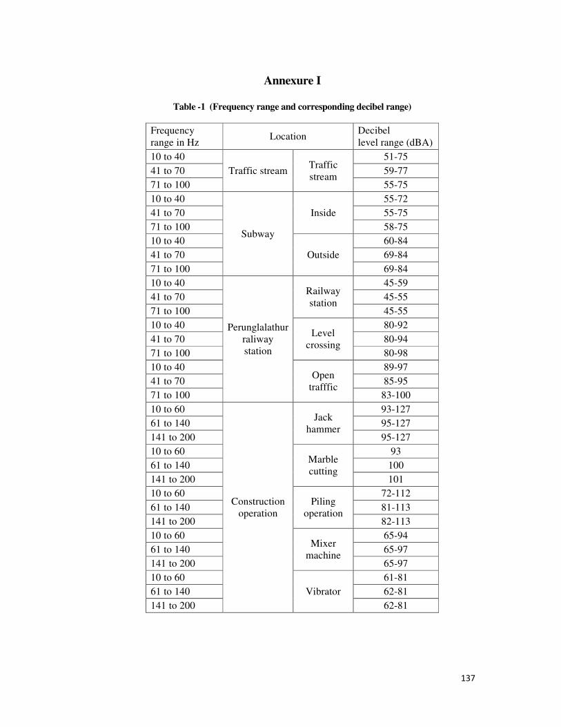
137

Annexure I

Table -1 (Frequency range and corresponding decibel range)

Frequency range in Hz

Location Decibel level range (dBA)

10 to 40

Traffic stream Traffic stream

51-75

41 to 70 59-77

71 to 100 55-75

10 to 40

Subway

Inside

55-72

41 to 70 55-75

71 to 100 58-75

10 to 40

Outside

60-84

41 to 70 69-84

71 to 100 69-84

10 to 40

Perunglalathur raliway station

Railway station

45-59

41 to 70 45-55

71 to 100 45-55

10 to 40 Level

crossing

80-92

41 to 70 80-94

71 to 100 80-98

10 to 40 Open

trafffic

89-97

41 to 70 85-95

71 to 100 83-100

10 to 60

Construction operation

Jack hammer

93-127

61 to 140 95-127

141 to 200 95-127

10 to 60 Marble cutting

93

61 to 140 100

141 to 200 101

10 to 60 Piling

operation

72-112

61 to 140 81-113

141 to 200 82-113

10 to 60 Mixer

machine

65-94

61 to 140 65-97

141 to 200 65-97

10 to 60

Vibrator

61-81

61 to 140 62-81

141 to 200 62-81

138

Annexure I

Table -1 (Frequency range and corresponding decibel range) contd.

Frequency range in Hz

Location Decibel level range (dBA)

10 to 40

Cars having different year

of manufacturing

2002 76-79

41 to 70 76-79 71 to 100 73-79 10 to 40

2004 62-77

41 to 70 70-77 71 to 100 69-79 10 to 40

2006 64-71

41 to 70 64-69 71 to 100 65-69 10 to 40

2008 64-66

41 to 70 66-68 71 to 100 62-68 10 to 40

2010 57-64

41 to 70 57-64 71 to 100 57-61 10 to 40

2012 55-59

41 to 70 55-59 71 to 100 55-59 10 to 40

Flour mills and

open traffic

Rice

90-98

41 to 70 90-94

71 to 100 90-94

10 to 40

Mirchi

105-115

41 to 70 105-115

71 to 100 108-115

10 to 40

Seekakai

90-98

41 to 70 90-94

71 to 100 90-94

10 to 40

OMR

58-83

41 to 70 51-74

71 to 100 55-82

10 to 40

KPR

47-61

41 to 70 45-60

71 to 100 48-60

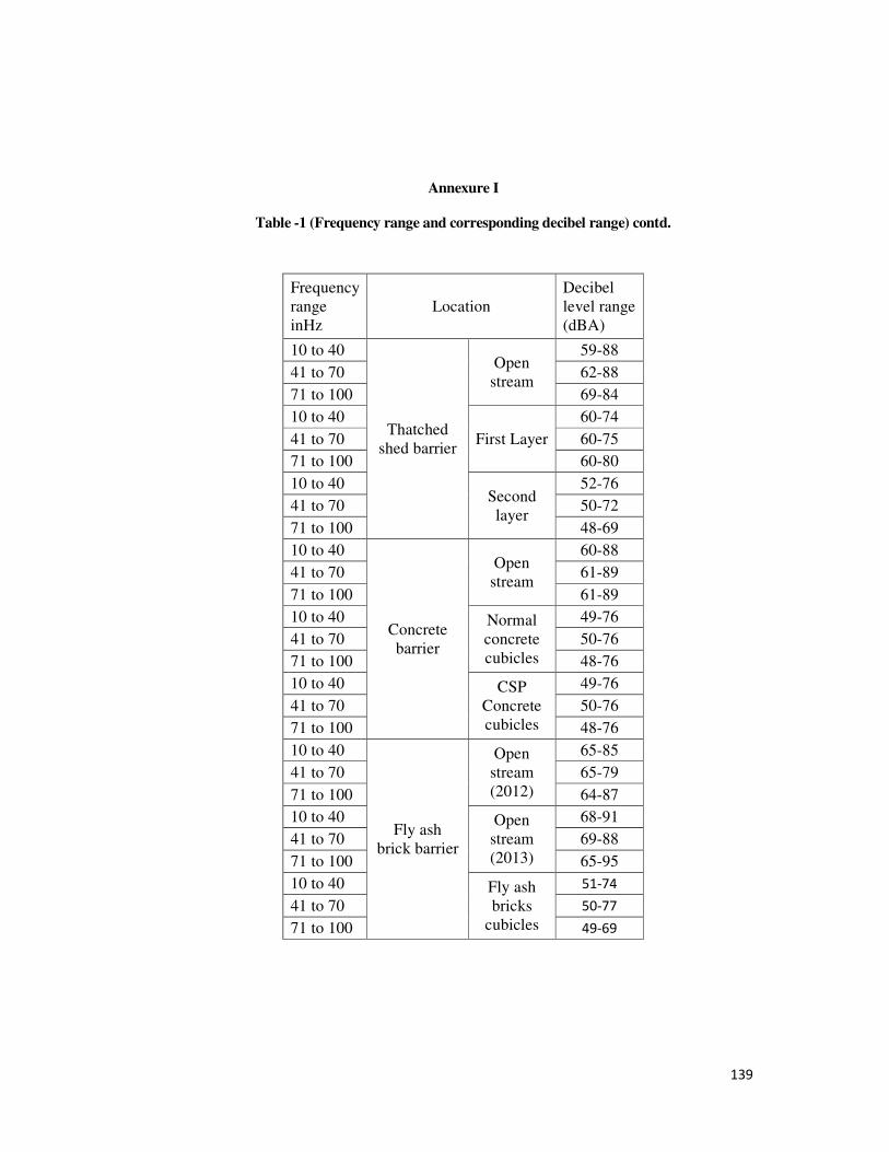
139

Annexure I

Table -1 (Frequency range and corresponding decibel range) contd.

Frequency range inHz

Location Decibel level range (dBA)

10 to 40

Thatched shed barrier

Open stream

59-88

41 to 70 62-88

71 to 100 69-84

10 to 40

First Layer

60-74

41 to 70 60-75

71 to 100 60-80

10 to 40 Second layer

52-76

41 to 70 50-72

71 to 100 48-69

10 to 40

Concrete barrier

Open stream

60-88

41 to 70 61-89

71 to 100 61-89

10 to 40 Normal concrete cubicles

49-76

41 to 70 50-76

71 to 100 48-76

10 to 40 CSP Concrete cubicles

49-76

41 to 70 50-76

71 to 100 48-76

10 to 40

Fly ash brick barrier

Open stream (2012)

65-85

41 to 70 65-79

71 to 100 64-87

10 to 40 Open stream (2013)

68-91

41 to 70 69-88

71 to 100 65-95

10 to 40 Fly ash bricks

cubicles

51‐74

41 to 70 50‐77

71 to 100 49‐69