Noise Levels in the American Sub-Arctic

PROCEEDINGS OF TIIE I.R.E.

Noise Levels in the American Sub-Arcticc*N. C. GERSONt

Summary-On the basis of six months' data, a comprehensivestudy was instituted of the atmospheric static intensity at a fre-quency of 150 kc in northern and southern Canada. Three noiselevels, the average (a measure of the mean atmospheric noise level),quasi peak (a measure of the highest noise bursts indicated by therecorder), and absolute quasi peak (a measure of the maximumvalue of the highest noise bursts indicated by the recorder) weredetermined. The average level furnished a record of the averagenoise caused by bursts and background rumble; the quasi-peaklevel of atmospherics furnished a record of noise bursts (superim-posed upon the usually negligible background); and the absolutequasi-peak level supplied the highest value of the bursts.

Various temporal and spatial distribution studies of the intensityof atmospherics were effected, such as diurnal, seasonal, latitudal,and the like. The diurnal trend is absent or small during winter butincreases markedly as summer is approached. The familiar rise anddecline of noise intensity about sunset and sunrise, respectively, isfound. Toward summer the increase in noise level rise occurs earlierand earlier, sometimes taking place shortly after noon, local standardtime (LST). The daily cycle usually attains a minimum after sunriseand a maximum after sunset, although exceptions are found.

Seasonally, the static intensity is higher in June than January.At southern stations noise increased progressively from January toJune.

A rise in recorded noise level above that of preceding and suc-ceeding months took place at some stations in February. The in-crease in noise level during this time is attributed to precipitationstatic caused by the increased frequency and force of blizzards.

The noise level varied as a nonlinear function of colatitude.

INTRODUCTION

fl[- HIS PAPER deals with the level of atmosphericsJI in the American sub-Arctic. Continuous measure-

ments were made during the six-month periodfrom January through June, 1947, at or near a frequencyof 150 kc at the stations of Baker Lake, Churchill, Ed-monton, Gloucester, Norman Wells, and Portage laPrairie, Canada (see Fig. 1). Technical details of theinstallation are showrn in Table I. In general, localsources of artificial man-made noise were lacking at allstations.

MEASUREMENT STANDARDIZATIONAlthough the procedure involved is very similar in

both cases, a determination of the atmospheric staticlevel nevertheless is beset with considerably more ob-stacles than is the measurement of radio field intensity.For example, the characteristics and wave forms of noisedisturbances vary tremendously since the various inte-grants are poorly defined and wildly fluctuating. Thesenoise components arrive at a particular point with vari-able polarization, amplitude, direction, relative phase,etc. Thus it is impossible, in most cases, to define an

* Decimal classification: R272.1. Original manuscript received bythe Institute, February 21, 1949; revised manuscript received,January 9, 1950.

t Air Force Cambridge Research Laboratories, Cambridge,Mass.

objective criterion of noise which may be convenientlyemployed as a standard of reference.

Fig. 1-Noise recorder station locations.

Heretofore, because of the above and other difficul-ties, the measurement of atmospherics at frequenciesbelow 5,000 kc had been considered satisfactory if results were reproducible to about 30 to 50 per cent withsimilar measuring devices.' When different types ofmeasuring instruments had been utilized to determinethe same noise level, results disagreed enormously, per-haps by as large a ratio as 1,000 to 1. It is believed thatwith the precautions and standardizations taken in thepresent study, the instruments and calibrating tech-niques were sufficiently consistent so as to reproducereadings within about 10 per cent.Undoubtedly a great portion of the disagreements

usually found when determining noise intensities lie inthe aforementioned erratic nature of atmospherics.However, a considerable degree of the encountered in-accuracy may be attributed directly to the instrumenta-tion. It is important, therefore, in order to insure uni-form, comparative, and meaningful results, to state

1 H. E. Dinger and H. G. Paine," Factors affecting the accuracyof radio noise meters," PROC. I.R.E., vol. 35, pp. 75-80; Januiary.1947.

9051950

PROCEEDINGS OF THIE I.R.E.

TABLE I

Station

Baker Lake, NorthwestTerritories

Churchill, Manitoba

Edmonton, Alberta

Gloucester, Ontario

Norman Wells, NorthwestTerritories

Portage la Prairie,Manitoba

Latitude Longitude(ON) (0w)

64018'56" 96002'1 7"

58056'57" 94011'38"

53033'46" 113°31'28"

45018'32 " 75030'50/"65016'29" 126046'56"

49°55'22" 981o6'53"

OperatingPersonnel*

RCCS

Antenna Sytem

59-foot vertical mast

RCN T antenna, 80-foot vertical.80-foot horizontal

RCAF 59-foot vertical mast

RCN T antenna, 80-foot vertical,80-foot horizontal



Ground System

Radial system 20- to 150-foot copperwires

Copper mat surrounding building


Ground system surrounding buildings


Copper mat; 20-foot lattice, approx-imately 200 feet square

* RCCS Royal Canadian Corps of Signals.RCN Royal Canadian Navy.RCAF Royal Canadian Air Force.

fully the instrumental techniques and procedures in-volved. This will be done after first reviewing the mostimportant factors which, in the measurement of noise,contribute to variations in the results.

Inaccuracies in noise mensuration at different loca-tions or at different times generally may be ascribed toone or more of the following factors:

1. Difference in the receiving antenna2. Difference in receiver characteristics, such as

(a) Bandwidth(b) Image response(c) Automatic volume control and weighting cir-

cuit constants(d) Insufficient shielding(e) Misalignment of radio-frequency circuits

3. Differences in the recording instrument4. Inaccuracies in the attenuator settings of the cali-

brating signal generator5. Operational variations:

(a) Variations in the power supply voltage(b) Variations in tube characteristics(c) Detuning of amplifier circuits by the M1iller

effect(d) Overloading and other nonlinear effects in the

receiver and/or recorcler6. Influences of personnel:

(a) Careless operation(b) Inexactness of calibration techniques.

To stanidardize the equipment and measuring meth-ods as much as possible and thus eliminate most of theabove variables, the followiing action was taken:

Standard anteinnas, 59-foot steel masts havinlg omni-direction reception characteristics, were employed wherepossible. At two stations, Gloucester and Churchill,weather or construction hindrances led to the utilizationof similar T antennas, each having about an 80-foot ver-tical and 80-foot horizontal section. The effective heightwas determined separately for each antenna.

Identical receivers operating at the same bandwidthwere employed.

Identical recorders were in use.Identical signal generators were employed. Accu-

racies of the attenuator steps were better than 10 percent.

Electronic- and saturation-type voltage regulatorswere employed. Radio tubes were changed periodically.

Careless operation and inaccurate calibration tech-niques were avoided to a great extent by training all op-erating personnel in the uniform procedures to be fol-lowed.

It is evident that the uncontrolled variables commonto all stations were located in the receiver, i.e., over-loading and other nonlinear effects, and detuning of theamplifier circuits by the Miller effect. It is believed,however, that the total effect due to these two factorsis very small. A further lack of standardization existed3at two of the stations where T antennas rather thansteel masts had been erected. Because of the flat top ointhe T antennas, and because noise rarelv, if ever, issolelIN vertically polarized, noise intensities as obtainedfrom the T antennas will be somewhat greater thanthose obtained from the steel rnasts under otherwiseidentical conditions. While the differences are believedto be small, their exact magnitudes are unknowni.

It is believed advisable to detail the instrumentationphases in order that future investigators may be ableto compare their restults with those given here.

ApparatusNote: The term "quasi-peak noise intensity" will be

employed for what nominally is termed the "peak inoiselevel." The true instantaneous highly peaked electro-magnetic noise wave in space is decreased in amplitudeduring reception because of the finite bandwidth of thereceiver. By introducing the phrase "quasi peak," theclistinction between the peak intensity as recorded andthe instantaneous highest intensity of the electromag-netic wave in space is emphasized.The noise-measuring equipment operated during this

test comprised an 18-tube superheterodyne receiver(Hammarlund Super Pro, Type BC-779-A) togetherwith an automatic recorder (Esterline Angus). The re-ceiver was modified to provide output voltages alter-nately proportional first to the quasi-peak and then tothe average value of the atmospheric noise field inten-sity. This was accomplished in the usual fashion by

906 A ugust

Gerson: Noise Levels in the Sub-A rctic

having the desired time constants in the receiver detec-tor circuit. Alternate recordings of the quasi-peak andaverage value of static were effected by means of a cam-operated relay.The receiver bandwidth was 2.42 kc. The charging

time constant of the average circuit was 98 seconds andthat of the quasi-peak circuit, 0.089 second. The re-corder, a continuously recording milliammeter, had anunshunted range of 0-5 milliammeters and a paper chartmovement of three inches per hour. Figs. 2 and 3 givethe receiver circuit diagram and, a block diagram show-ing the equipment arrangement, respectively.

OUTPUT2 ND. I.F.

4(L E A KA DJ.

GRID RET.2ND. I.F.

A.V.C.

VOLTAGE

V. T. V ..M.

Fig. 2 Receiver circuit diagram.

7V

HAMMARLUND ESTERLINESUPER-PRO ANGUSRECEIVER RECORDER

Fig. 3-Block diagram of arrangement of equipment.

In calibrating the apparatus in its quasi-peak record-ing position, it was decided to employ not a continuous-wave signal but a signal which simulated a typical noiseburst. Since the best approximation to a noise burst,i.e., a delta function, is difficult to attain in practice, a

compromise was adopted in the form of a trap)ezoidal250-microsecond pulse having a recurrence rate of 25per second. Inasmuch as receiver response is not nec-essarily the same for a sinusoidal as for a pulsed input,and since noise in a great many instances is of an im-pulsive or crashy nature, the pulse calibration procedureappeared more logical than that of employing modu-lated continuous waves. The wave form of atmosphericbursts was not duplicated; nevertheless, the utilizationof pulses rather than continuous-wave signals allowedthe receiver to be calibrated under conditions whichmore closely approached those encountered in actual op-eration. The pulse calibration was employed with thequasi-peak recording circuit. Conversely, when cali-brating the average recording position, a continuous-wave modulated signal was employed.A portable transmitter, radiating a 250-microsecollnd

pulse at a recurrence rate of 25 per seconid, and a fieldintensity meter designed for the measurement of pulseamplitudes at low frequencies were employed to de-termine the antenna constants.The equipment was calibrated in the usual manner.

Deflections of the noise recorder for a series of givensignal generator outputs provided convenient "abstrac-tion scales," by means of which the noise levels could beabstracted from the record. Two abstraction scales wereprovided daily: a "peak-pulse" scale indicating that thereceiver peak RC circuit was calibrated with the pulsedsignal described above, and an "average continuouswave" scale indicating that the receiver average RCcircuit was calibrated with a continuous-wave signal.

EVALUATION

The noise charts as received provided a wealth ofminutia regarding temporal noise fluctuations, but intheir recorded form they were mathematically rigid aindnot amenable to systematic compilation. Before centraltendencies, trends, or correlations could be obtained, itwas essential to convert the recorded data into a formsuitable for statistical manipulation. The evaluationencompassed three phases: abstraction, reduction, andrepresentation.

A bstractionEmploying the abstractioni or calibrationi scales pro-

vided daily, three sets of data were removed from therecord for each hour: the mean average noise level, themean quasi-peak noise level, and the maximum or abso-lute quasi-peak noise level. The mean value was thearithmetic mean of the data for the hour considered andthe "absolute" value was the maximum which was re-corded during that hour. The "average continuouswave" (an average continuous-wave input signal to thereceiver) calibration scale was employed to abstractaverage noise and the "peak-pulse" (a pulsed input sig-nal to the receiver) calibration scale to abstract quasi-peak noise. The data were tabulated by hours of the dayon a monthly basis.

1950 9M07

PROCEEDINGS OF HIIE I.R.E.

Reduction

Inasmuch as the static levels present occasionialgreatly outlying values, considerations of the desideratafor a satisfactory central tendency led to the choice ofthe median2 as the best measure for the investigation athand. The median is more stable and less affected bysampling fluctuations when, as in the case of atmos-

lherics, magnitudes surge from low or moderate to ex-

tremely high values and then recede. As justifiable ex-

tensions of the median, the third quartile3 and the maxi-mum (or highest) values were also chosen to representthe data.A second but less important reason for employing the

several quartile values arises from the nature of thedata. The lower values of recorded noise are so low thatthey appear to indicate thermal noise of the receiverrather than true natural noise levels. In these instances,by excluding lower decile magnitudes, third or fourthquartiles provide a better portrayal of the data.The median, third quartile, and maximum hourly

noise values were obtained for each hour of the day con-

sidering that same hour of each day in the month.Values were obtained from at least twenty samples atall stations except at Baker Lake, where, particularlyduring February and April, 1947, the number of ob-servations occasionally dropped to ten.The quartiles of noise strength were reduced from

microvolts receiver input to microvolts per meter atuInit bandwidth through the use of the relationship

M = Q/aB112

where Al1= quartile value of noise field intensity (micro-volts per meter), a = antenna constant (meter), B = re-

ceiver bandxx-idth (kc), and Q=quartile value of re-

corded noise (microvolts receiver input).

Representation

Quartiles of the meani average, mean quasi-peak andabsolute quasi-peak level of atmospherics are portrayedon a monthly basis for each station as quotidian, con-

tinental, and latitudinal variations.

DISCUSSION OF RESULTSGeneral

Undoubtedly the greatest portion of terrestrial atmos-pherics is generated in thunderstorms, probably by thetransformation of heat energy (released by condensingwater vapor) into mechanical energy (manifested bywinds and turbulence) and subsequently into electricalenergy (revealed by the production and separation of

2 For a set of observations arranged in order of imagnitude, themedian is defined as the middle value if there is one, otherwise as theinterpolated middle value. Thus, half the values are smaller than themedian and half the values are greater than the median.

I If a set of observations are arranged in order of magnitude anddivided into four equal parts, the points of division are known as

quartiles. The second quartile is identical with the median. Thusthree-fourths of the observations are smaller in magnitude than thethird quartile.

charged particles). Two other possible sources of ter-restrial radio noise are also known: (1) storms of blowingparticles that generate electric charges and potentialgradients, and (2) random noise caused by high electro-static fields between the ground and the air immediateIN,above it. On the average, the static produced by thelatter two sources is normally much smaller than thatcaused by thunderstorm activity. However, when excep-tionally large potential gradients exist, the noise pro-duced by the resulting local corona discharge may easilyexceed that due to distant thunderstorms.

In general, the geographical source regioni of a verygreat portion of the radio static observed in middle andhigher latitudes lies in the tropics or semitropics wherethe frequency of thunderstorms is greatest.4

Several admonitory remarks are necessary to insurethat no misinterpretation of the data will result.

1. Set noise placed a lower limit to the sensitivity ofthe equipment. If a diurnal trencl is absent, naturalnoise intensities are probably below those shown.

2. A small diurnal change probably indicates that setnoise exceeded the lower portions of the daily vari-ation.

3. The data represent noise intensities for the periodfrom January through June, 1947. However, theexceptionally large sunspot activity during this pe-riod may have colored the results.

4. Maximum absolute quasi-peak5 antcI mean quLasi-peak6 noise values during winter more closelyapproximate the true tend than do the medians.

5. The detection of noise may be made (a) by ob-servation of an oscilloscope, (b) by aural percep-tion wherein an observer listens to the receivednoise, or (c) by a meter. The results in each casemay be quite differenit because of differences in theequipment and the senises involved. For example,the recovery of the eye (viewing an oscilloscope) toa noise burst is far superior to the ear hearing thesame bursts. In the present instance, noise was re-corded by meter.

Diurnal Noise Variation

Curves portraying the (liurnial noise initenisity varia-tion are shown in Figs. 4 through 12.

In each figure, a heavy solidl curve indcicates themaximurm value of the variable; a heavycdashed curve,the third quartile; and a light solid curve, the medliani.A heavy solid line is drawn at the top of the diagrami toportray the hours of darkness, the beginning indicatiingsunset and the ending indicating sunrise. Whenever, be-cause of limitations in the apparatus, the recorder penswung off scale, a heavy dot was plotted on the graphat the value at which the pen wxent off scale. A dot thus

4F. A. Berry, E. Bollay, and N. R. Beers, "Handbook of Meteor-ology," McGraw-Hill Book Co., New York, N. Y., p. 995; 1945.

5 The highest value considering only a series of the highest hourlynoise values.

6 The arithmetic mean of a series of average hoturly quasi-peaknoise values.

9()8 A ugus t

Gerson: Noise Levels in the Sub-Arctic

signifies that the true noise level is to some unknownextent higher than the indicated value. If a sufficientnumber of such instances occurred during the month,it was possible for the third quartile or median to be anoff-scale value. When the median was an off-scale value,then, since obviously both the third quartile and maxi-mum values likewise were off-scale, one dot was plottedfor all three measures. The microvolt-per-meter scalevalues were chosen to afford as uniform a representation

& 0.5

5oo .-,

1000

500

50

A J",

AI"I/It-/

as possible. Noise levels which appear at the very bot-tom of the graph may be somewhat lower than depicted.The subsequent discussion will deal primarily with

the mean quasi-peak noise level. It will be found that ina great majority of instances, the variations, trends, andthe like, of the mean average and the absolute quasi-peak static intensities will be similar or identical to thoseof the mean quasi peak.From an analysis of the data, several general features

11 IjI J. I I. ..I l I Ij II

00 0 . 16 20 24 04 08 12 16 20 2400 04 08 12 2024004 08 2 6 20 24 00 04 08 10 16 20 24

Fig. 4-Hourly mean average and mean quasi-peak noise intensity (January through June, 1947), Baker Lake, Northwest Territories.

MEAN AVERAGENOISE INTENSITY

MAXI MUM----THIRD QUARTILE

-MEDIAN

00 04 08 12 16 20 24 00 0MAR GMT

- I,r IT-CHURCHILL, MANITOBA

1- t--t

7___

I'-Jl

2 1,DR

vV

.1A

SLVAVIj0 24 00 04 0 12 20 4 00 04 08 12 12 0 24

MA" JUNE

i_ MEAN QUASI-PEAK .|| |[ r X- Xg- -I ---NOISE INTENSITY

~ ~~ ~ ~ ~ ~ ~ ~ ~ -

F --- 1- 1- 1At1 1 1 t I 1-

'-A~~~~~~~~~'

120 24100 2 202400 04 01 12 18 2024100 04 0 12 18 2 2400 04 08

Fig. 5-Hourly mean average and mean quasi-peak noise intensity (January through June, 1947), Churchill, Manitoba.

1950 909

2A 16 20 24A

1--- _1-\I --t

10 20 24

0

8..I

S /

'°I

Vo--I,5 00 0 1<

s ool 04

I

.1 _

- /

00 04 08 12FES

A4 I_,,v"rv

00 04 08 2 a

I0°°l506 1

f%

00 04 08

-

x-

0 -24 C(

S/

N/

A'VI

F.

-

05001-

(6

PROCEEDINGS OF T'HE I.R.E.

are immediately evideiit. For the different months atthe several stations, diurnal variations are similar, es-

pecially with regard to the greater nccturnal than day-light intensity of noise. Also, during winter the start ofhigh nighttime static levels closely coincides with thearrival of sunset at the receiving station.The mean average noise level curves do not reveal a

diurnal variation during winter. The lack of an observa-ble trend does not imply that the variation is absent,

but merely that the average level of atmospheric noisewas of such a low intensity that it is obscured by setnoise. Although the curves fail to reveal true noise levels,nevertheless they do indicate an upper limit to levels ofaverage atmospheric noise which might be encouinteredat the location in question.The diurnal cycle, which was lacking in the mean

average noise data, evinces itself in the mean quasi-peak (from about March onwards) and absolute quasi-

100__=__.

50~~~~~~~~~~~I

0.5

i 0 04 OB 12 16 20 242 ~~~~~JAN.

\10 - -,-I5 _

IA

-_N

t00 04 08 12FEB,

_ =

IJ' x,

00 04 08 2

M EAN AVERAG ENOISE INTENSITY

MAXIMUM-THIRD OUARTILE-MEDIAN

-== =

00 04 08 12 16 20 24 (MAR. G. M.

MEAN OUASI-PEAK| NOISE INTENSITY

100o 014 -08 ~ L.1 20 74

16 21PR.

AV

'O 24

04 Ol 12 I6 20 24 00 0

\

I 1

00 04 oR 12 I6 20 24JUNE

00 04 08 12 16 20 24

Fig. 6-Hourly mean average and mean quasi-peak noise intensity (January through June, 1947), Edmonton, Alberta.

MEAN AVERAGE

NOISE INTENSITY

-_---THIRD QUARTILE

~MEDIAN

R08 2 16 20 24 00 04 08 12 16 20 24 00 04 08 12 16 20 24 00 04 08 12 16 20 24 00 04 08 12 16 20 24 00 04 08 12 IC

JAN FER MAR G. M.T M APR MMAY JUNE

NOISE INTENSITY

lili)4 08 12 16 20 24 00 04 08 I2 IN 20 24 00 04 08 12 16 20 24 00 04 08 12 16 20 24 00 04 oR 12 16 20 24 00 04 08 12 16 20 24

Fig. 7-Hourly mean average and mean quasi-peak noise intensity (January through June, 1947), Gloucester, Ontario.

910 A ugust

i

!40

JL!40

\ P,-5-,.v

4

00 04 08 I,,W

I

-j

2 16 20 24L

II'-II

.j /II

16 20 24

16 20 2, 00 0,I.T. .

-l/1--

00 0,

08 i:

1

0816 20 2420 24_ -

-00 04 08 12 11

I


peak curves (from January at some stations). The dailyvariation appears if not in the median then in the maxi-mum values. During January and February, meanquasi-peak graphs indicated a diurnal trend, to someextent, at all stations except Norman Wells.As the seasons progressed, the diurnal noise cycle

showed certain progressive changes. The amplitude ofthe daily cycle and the magnitude of the static, whichwere very small in winter, became greater and greater

as the summer solstice was approached, reaching itsmaximum during June.From climatological considerations, it is believed

that the static intensity probably would culminateduring July, after which the reverse effect, i.e., a graduallowering of both the level of noise intensity and thediurnal variation, would occur until a minimum wasreached in January and February. It should be notedthat months equially spaced on either side of abotut July

C

D0 04 08 12 Is 20 24FES

00 04 08 12 la 2

MiAR

_I

u1/\1 I

D 1 4 00 04 08 12 Is 20 Z4G.M.T APR

J Q MEAN QUASI-PEAKll |NOiSE INTENSITY

A} 1- i1'Il

00 04 08 12 16 20 24M1AY

II-l l

I K __X_ __

00 04 18 12 16 20 24 00 04 oe 12 16 20 24 0 004 08 12 112162400 04 0d12 16 2824

Fig. 8-Hourly mean average and mean quasi-peak noise intensity (January through June, 1947), Norman WTells,

a

I

7.'

MEAN AVERAGENOISE INTENSITY

MAXIMUMTHIRO QUARTILE

- MEDIAN

IlSI

00 0

r

914 c

Northwest Territories.

47%.-2

I

74

JAN. FE. RUT. APR. MAY JUNE

PORTAGE LA PRAIRIE, MANITOBA

MEAN QUASI-PEAK

NOISE INTENSITY

100

.. . ... . .

50

0004 I w 00 04 la 16 0 2 4a 04 16 so4G0 04 08 a B6 100 @4 0e 0o 240004 08 12 20 24

Fig. 9-Hourly mean average and mean quasi-peak noise intensity (January through June, 1947), Portage la Prairie, Manitoba.

1950 911

r2I I00

'0 0

O 000

:E 500

- .-

i

-r\^

NE12

I-^.-I

I

Is2JAN

lool

1--.,N

a

,'aI

PROCEEDINGS OF THE I.R.E.

I would not necessarily have the same noise intensityand quotidian variation because of the quantitativelyunpredictable effect of sunspot, magnetic, meteoro-logical, and other influences.A progressive change occurs in the diurnal variations

of noise intensity as summer approximates. DuringJanuary, February, and March, atmospherics begiii torise about sunset and attain maximumi magnitudes sev-eral hours later (luring the night. A reduction of noise

commences, in general, several hours prior to sunrise,attaining minimum values at about dawn. This effectis best typified by the mean quasi-peak curves forGloucester, and also several other stations (see Figs. 5,6, 7, and 9).As June approaches, the transition towards noc-

turnal static levels begins earlier and earlier with re-spect to sunset. Conversely, the decline from highnightly noise intensity towards the appreciably lower

I

Fig. 10 Hourly absolute quasi-peak noise intensity (January through Juine, 1947), Baker Lake, Northwest Territories,and Churchill, Manitoba.

Fig. 11-Hourly absolute quasi-peak noise intensity (January through June, 1947), Edmonton, Alberta, and Gloucester, Ontario.

9t August

.00 04 0 a 12 16 20 24JUNE

Gerson: Noise Levels in the Sub-Arctic

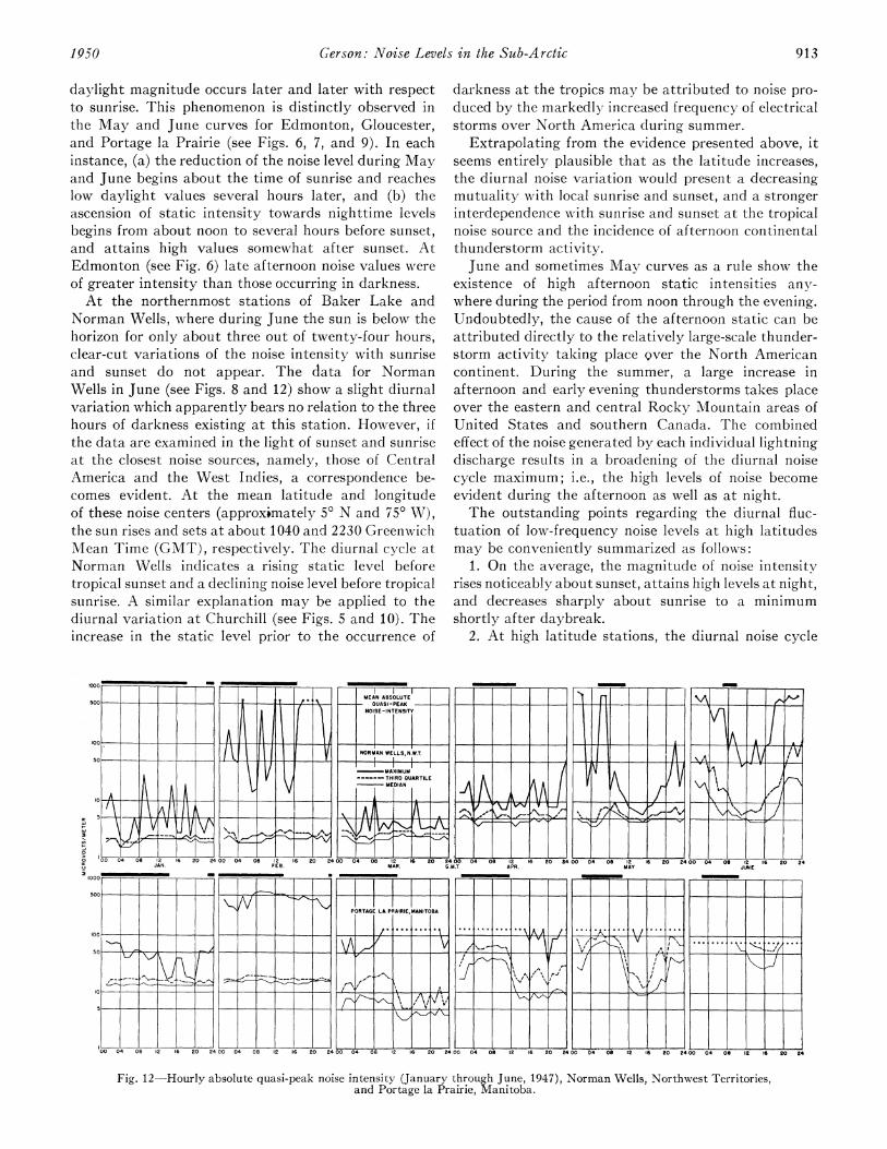
daylight magnitude occurs later and later with respectto sunrise. This phenomenon is distinctly observed inthe May and June curves for Edmonton, Gloucester,and Portage la Prairie (see Figs. 6, 7, and 9). In eachinstance, (a) the reduction of the noise level during Mayand June begins about the time of sunrise and reacheslow daylight values several hours later, and (b) theascension of static intensity towards nighttime levelsbegins from about noon to several hours before sunset,and attains high values somewhat after sunset. AtEdmonton (see Fig. 6) late afternoon noise values wereof greater intensity than those occurring in darkness.At the northernmost stations of Baker Lake and

Norman Wells, where during June the sun is below thehorizon for only about three out of twenty-four hours,clear-cut variations of the noise intensity with sunriseand sunset do not appear. The data for NormanWells in June (see Figs. 8 and 12) show a slight diurnalvariation which apparently bears no relation to the threehours of darkness existing at this station. However, ifthe data are examined in the light of sunset and sunriseat the closest noise sources, namely, those of CentralAmerica and the West Indies, a correspondence be-comes evident. At the mean latitude and lotngitudeof these noise centers (approximately 50 N and 750 W),the sun rises and sets at about 1040 and 2230 GreenwichMean Time (GMT), respectively. The diurnal cycle atNorman Wells indicates a rising static level beforetropical sunset and a declining noise level before tropicalsunrise. A similar explanation may be applied to thediurnal variation at Churchill (see Figs. 5 and 10). Theincrease in the static level prior to the occurrence of

500 -

16 20 24 00 04 08

darkness at the tropics may be attributed to noise pro-duced by the markedly increased frequency of electricalstorms over North America during summer.

Extrapolating from the evidence presented above, itseems entirely plausible that as the latitude increases,the diurnal noise variation would present a decreasingmutuality with local sunrise and sunset, and a strongerinterdependence with sunrise and sunset at the tropicalnoise source and the incidence of afternoon continentalthunderstorm activity.June and sometimes May curves as a rule show the

existence of high afternoon static intensities anv-where during the period from noon through the evening.Undoubtedly, the cause of the afternoon static can beattributed directly to the relatively large-scale thunder-storm activity taking place over the North Americancontinent. During the summer, a large increase inafternoon and early evening thunderstorms takes placeover the eastern and central Rocky Mountain areas ofUnited States and southern Canada. The combinedeffect of the noise generated by each individual lightningdischarge results in a broadening of the diurnal noisecycle maximum; i.e., the high levels of noise becomeevident during the afternoon as well as at night.The outstanding poiInts regarding the diurnal fluc-

tuation of low-frequency noise levels at high latitudesmay be conveniently summarized as follows:

1. On the average, the magnitude of noise intensitvrises noticeably about sunset, attains high levels at night,and decreases sharply about sunrise to a minimumshortly after daybreak.

2. At high latitude stations, the diurnal noise cycle

20 24

Fig. 12-Hourly absolute quasi-peak noise intensity (January through June, 1947), Norman Wells, Northwest Territories,and Portage la Prairie, Manitoba.

PORTAGE LA PRAIRIElMANITOBA

'2 16 2 24...

2 1A 20 24 00 04 08 !2 16 20 24 00 04 08 12 16 20 24 00 04 08 12 16 20 2400 04 08

1950 913

us

>

cr

I0001

-:~1001

50

51

1100 04 081 2 1,


during summer apparently bears no simple relationshipto local sunrise and sunset. The evidence indicates arelationship with sunrise and sunset at the tropicalcenters generating the noise and with the time of oc-currence of continental afternoon thunderstorms.

3. The rise to nocturnal high noise levels occurs earlierwith respect to sunset, and the decline from high nightlystatic to low daylight values occurs later with respect tosunrise in summer than in winter.

4. Broad maxima of noise extending from shortlyafter noon into darkness appear during the summer. Thenoise is traceable to vigorous thunderstorm activityover the North American continent during this season.

5. No diurnal trend is manifest during winter at theiiorthernly stations. Set noise in this region apparentlyis appreciably higher than the mean average static level.

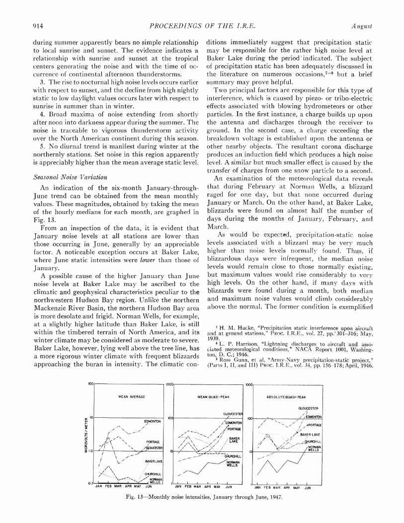
Seasonal Noise VariationAn indication of the six-month January-through-

June trend can be obtained from the mean monthlyvalues. These magnitudes, obtained by taking the meanof the hourly medians for each month, are graphed inFig. 13.From an inspection of the data, it is evident that

January noise levels at all stations are lower thanthose occurring in June, generally by an appreciablefactor. A noticeable exception occurs at Baker Lake,where June static intensities were lower than those ofJanuary.A possible cause of the higher January than Junie

noise levels at Baker Lake may be ascribed to theclimatic and geophysical characteristics peculiar to thenorthwestern Hudson Bay region. Unlike the northernMackenzie River Basin, the northern Hudson Bay areais more desolate and frigid. Norman Wells, for example,at a slightly higher latitude than Baker Lake, is stillwithin the timbered terrain of North America, and itswinter climate may be considered as moderate to severe.Baker Lake, however, lying well above the tree line, hasa more rigorous winter climate with frequent blizzardsapproaching the buran in intensity. The climatic con-

ditions immediately suggest that precipitation staticmay be responsible for the rather high noise level atBaker Lake during the period indicated. lThe subjectof precipitation static has been adequately discussed inthe literature on numerous occasions,7-9 but a briefsummary may prove helpful.Two principal factors are responsible for this type of

interference, which is caused by piezo- or tribo-electriceffects associated with blowing hydrometeors or otherparticles. In the first instance, a charge builds up uponthe antenna and discharges through the receiver toground. In the second case, a charge exceeding thebreakdown voltage is established uponI the antenna orother nearby objects. The resultant corona dischargeproduces an induction field which produces a high noiselevel. A similar but much smaller effect is caused by thetransfer of charges from one snow particle to a second.An examination of the meteorological data reveals

that during February at Norman Wells, a blizzardraged for one day, but that none occurred duringJanuary or March. On the other hand, at Baker Lake,blizzards were found on almost half the number ofdays during the months of January, February, andMarch.

As would be expected, precipitation-static noiselevels associated with a blizzard may be very muchhigher than noise levels normallyr found. Thus, ifblizzardous days were infreqtuent, the median nioiselevels would remain close to those normally existinig,but maximum values would rise considerably to veryhigh levels. On the other hand, if many days withblizzards were found during a month, both medianand maximum noise values would climb considerablyabove the normal. The former condition is exemplifiedl

I H. M. Hucke, "Precipitation static interference upon aircraftatnd at ground stations," PROC. I.R.E., vol. 27, pp.-301-316; May,1939.

8 L. P. Harrison, "Lightning discharges to aircraft and asso-ciated meteorological conditions," NACA Report 1001, Washing-ton, D. C.; 1946.

9 Ross Gunn, et al, "Armiiy-Navy precipitation-static project,"(Parts I, II, and III) PROC. I.R.E., vol. 34, pp. 156-178; April, 1946.

100

MEAN AVERAGE

r 10EDMONTON

E .

PORTAGE

\ X~ %/GOUCESTER

/ BAKER LAKE

~~~~CHURGHILL

NORMAN

~~~~~WELLSJ.AJAN FEB MAR APR MAY JUN

1000

10C

10

MEAN QUASI-PEAK

GLOUCESTER

,/EDMONTON/ 'PORTAGE

BAKER/\ 'I ~~LAKE

/, \\ ..- .,

- CHURCHILL

_,NORMANWELLS

'°°r,

100

10-

JAN FEB MAR APR MAY JUN

ABSOLUTE QUASI- PEAK

GLOUCESTER/S-. ,/EDMONTON

- -I/ PORTAGE

- BAKER LAKE

/} \ ,:/ __ CHURCHILL

+,/z, .,' NORMANWELLS

IJJAN FEB MAR APR MAY JUN

Fig. 13-Monthly noise intensities, January through June, 1947.

cr

914 A ugust


by Norman Wells in February and the latter by BakerLake during January, February, and March, wherethirteen blizzardy days were found during each month.A similar situation was found at other stations

(Churchill, Gloucester, and Portage la Prairie) wherethe noise level during February exceeded that duringJanuary or March. This increase in static noise level isimputed to the more frequent and more vigorousstorms of blowing snow usually found in the month ofFebruary.With the onset of spring conditions, in April, the

number of blizzards fell off sharply, thereby removingthe local level of atmospherics. After this time, naturalnoise was probably that propagated from the tropicsand the thunderstorm areas of the continent.

During the summer, the more southerly stationsindicated the high and somewhat erratic daily noiseintensity trend which is characteristically found atlocalities not too distant from thunderstorm activity.Since June is one of the summer months during whichlocal electrical storms contribute substantially to thetotal noise level, the daily curves may show relativelylarge noise-level fluctuations, depending uipon the ab-sence or presence of such a storm.

In general, the mean average noise field intensity isat a much lower level at all stations considered than forstations in the temperate zones.A general increase in noise from winter to summer is

found also in the mean quasi-peak and absolute quasi-peak maps (see section on Continental Noise Variation).At the southern stations, mean monthly quasi-peaknoise intensities exceed 100 microvolts per meter during

June, but only about 25 microvolts per meter duringJanuary. It is interesting to note the increased noiselevel in February above that of both January andMarch. The cause for this rise is believed to be precipita-tion static.The absolute quasi-peak noise intensity maps pro-

vide an indication of the noise levels to be overcome ifcommunication is desired at all times at a frequencyof 150 kc.

Continental Noise VariationValues of mean monthly noise intensity at each

station -have been plotted on maps of North Americafor the six-month interval (see Fig. 14).

It is seen that the mean average monthly values forthose stations located above 550 N latitude was lessthan one microvolt per meter throughout the periodl.On the whole, the very small variation disclosed iindi-cates that set noise was probably the limiting factor.At the stations below 550 N latitude, noise rose gradu-ally from January to June. Throughout the entire periodthe mean average monthly noise level was less than 10microvolts per meter at all stations.

Variation of Noise with LatitudeIt is evident that under the supposition that the

tropical belt is the general center of terrestrial staticgeneration, at least for the longer wavelengths, noiselevels for a given low frequency should vary inverselywith latituLde. Some investigators have proposed a nega-tive linear latitude trend for the noise-latitudle rela-tionship.

JAN. FEB. MAR. APR. MAY JUNE

Montt,ly Mean Averoge Noise Intensities (Microvolts/Meter)

IF J*

" . j

6

C'. V.IV"O

64.

-;. .11

't4%'ZO, -U.,c "

,lk ll.f

Monthly Mean Ouasi - Peak Nois lntensltlesoCMcrovolts/ Meter)

Absolute Quasi-Peak Noise Intens ities (Microvolts/Meter)

Fig. 14-Monthly noise intensities (maps), January through June, 1947.

1950 915


At high latitudes, noise levels are exceptionally low.In addition to the very low intensities found in thisstudy, an independent research body made the follow-ing qualitative conclusion:10 "Measurements were at-tempted at Crystal No. 2, Baffin Island (latitude 63° N,longitude 68° 30' W) for only a short period but becausethe verv low natural static noise level was found to bebelow the level of local man-made noise, the measure-ments were not continued." These observations weremade at a frequency of 170 kc.

In an attempt to determine the variability of at-mospherics as a function of latitude, the relative in-tensities of the observed noise for all months wereplotted as ordinates against degrees of latitude asabscissas (see Fig. 15). The relative intensity was ob-tained by normalizing the results of the mean quasi-peak noise level on those of the southernmost station,Gloucester, considered as unity.

2.5

2.0 <

wr 4Cw

0

z YEG P

15Z 0 cr

0_ .5 WIT a:TI :

z 0 cr 2 Yc-0 0 a 0 70

w ( L0.W 0 lmZ

0

crCOMPUTED

0.5 WITH AUSTINCOHEN FORMULA *

0.40' 50' 60' 70.

LATITUDE

Fi-. 15-Variation of noise intensity with latitude.

It is apparent that the relative noise intensity atBaker Lake is not in keeping with the trend at theremaining stations, but is higher. Because of the singularlocal conditions at this station, it had already been con-cluded that winter noise intensity at Baker Lake wasappreciably influenced by precipitation static, andtherefore was greater than that which would be ex-pected if the tropical noise center were the sole noisesource. For this reason, the relative noise intensities atBaker Lake will be ignored and only noise levels at theremaining locations will be discussed.

In examining the trend of noise versus latitude, alinear relationship is not evident. Such a relationshipshould hardly be expected, especially at the higherlatitudes, if tropical regions are considered as thesource of a major proportion of atmospherics.

Since the stations concerned in this investigation arelocated at high latitudes, it was felt that a reasonablefirst approximation to the expected noise variation

10 Report ORS-P- 23, Office of Chief Signal Officer, U. S. Army,Washington, D.C., p. 103; 1945.

with latitude could be obtained through the use of theAustin-Cohen formula for the propagation of daytimesky-wave signal strengths. At the distances involved,tropical noise received at the recording stations wastransmitted via the ionosphere and was thus entirelysky wave. The semi-empirical Austin-Cohen relation-ship for attenuation may be written

E = (3 X 105/R)(P/O sin 0)112e-kl

where k =46X 10-6f06R, E=field intensity (microvoltsper meter), R = radius of earth (km), P = radiated power(kw), 0 = arc of earth from radiator to receiver (radians),and f =frequency (kc).The relative intensity at latitudes 00 and 0 of a given

noise signal radiated at the equator is, therefore, givenby

E/Eo = [Oo(sin Oo)/O(sin 0) ]1/2ek(O -O.

In order to compare data calculated from the aboveequation with those already plotted in Fig. 15, Go wastaken for the latitude of Gloucester (Oo =4518'32"). Inthe evaluation, the constants f and R were taken asf= 150 kc and R = 6367.6 km.

The important sources of atmospherics received overa major portion of North America are located in theWest Indies and equatorial South America. A "centerof gravity" for the combined regions of radio noise pro-duction may be taken as between latitudes 50 N to 100 N.For the purpose of this discussion, the noise was takenas originating at 100 N. Simple computation, however,will reveal that a choice of 50 N as the source of noisewould given no appreciable deviation from the results tobe described.A graph of the received relative signal (or noise)

levels for a signal transmitted at 100 N, consideringthe field intensity at Gloucester as unity, is shown asthe heavy solid curve in Fig. 15. The fit of the curve tothe observed data appears to indicate that the assump-tions employed are closely true.

ACKNOWLEDGMENTS

Original impetus for this study was supplied by theestablishment of the experimental low-frequency lorannetwork in southern Canada.The author is pleased to acknowledge the valuable

comments and criticisms of Lt. Col. G. M. Higginson,USAF, and S. L. Seaton, and the invaluable field as-sistance of H. J. Doane. The study itself could not havebeen accomplished without the painstaking care andhelp of Miss Alta Schoettle, 0. W. Armstrong, M. W.Begala, A. J. Beauchamp, J. Hoffman, L. D. Hogan, M.Setrin, M. S. Kelemen, E. T. Smith, Mrs. R. Halliday,and many others too numerous to mention. Finally,the author wishes to thank V. S. Carson for his constantencouragement.

916 A ugust

Documents

Noise Levels in the American Sub-Arctic