Noise Analysis v.21

8/8/2019 Noise Analysis v.21

http://slidepdf.com/reader/full/noise-analysis-v21 1/13

Noise Analysis of fceo-stabilized Lasers

Version 2.0

Basic Formulas in Noise Analysis:

Given an ergodic random process n(t):

The variance of the random process can be calculated from the time series or the

probability density:

∫ −∞→

=T

T T

dt t n

T

t n )(

2

1)( 22

lim

dnn f nt n E t n )(})({)( 222 ∫ ∞

∞−

==

Where E{X} denotes the expected value of the random variable X. The power spectral

density )( ω jS nn is the fourier transform of the Autocorrelation function

)}()({)( t nt n E Rnn τ τ +=

τ τ ω ωτ

d e R jS j

nn xx

−∞

∞−∫ = )()(

The power spectral density integrated over the entire spectrum yields the variance of the

process, which is also the average power of the signal.

== ∫ ∞

∞−

ω ω π

d jS t n xx )(2

1)(2 average power

For the following it is important to understand how power spectral densities of quantities

are changed when the signal propagates through a linear time invariant system (LTI-

system). Let the input signal be x(t) and the output signal be y(t). The system is described

either by its impulse response h(t) or frequency response )(ω

j H , which are Fourier transforms of each other

dt et h j H t jω

ω −

∞

∞−∫ = )()(

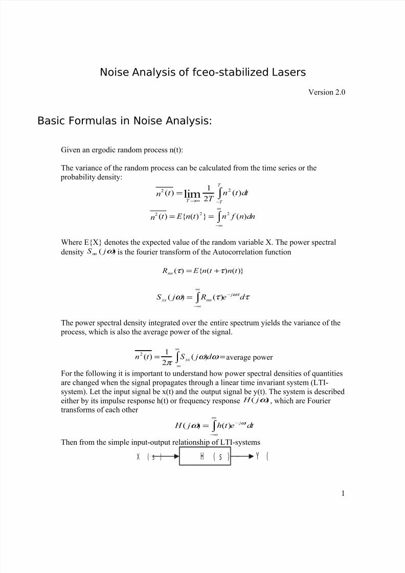
Then from the simple input-output relationship of LTI-systems

H ( s )X ( s ) Y (

1



we obtain)(*)(*)()( τ τ τ τ −= hh R R xx yy

or in the frequency domain we obtain for the spectra

)(*)()(2

ω ω ω jS j H jS xx yy = .

Simple feedback analysis

F

F

F

B

X Y+

with Black’s formula

)()()( s X s F sY =

)()(1

)()(

s F s F

s F s F

B F

F

−=

Easy to remember: The transfer function of a feedback loop is the forward gain devided by 1- minus the loop gain. The important property to realize is, that if the forward gain is

large, 1)()( >> s F s F B F , the loop transfer function

)(

1)(

s F s F

B

−=

independent of the forward gain (eventually even nonlinear, temperature sensitive,……)!!!!

2



System block diagram

The fceo-stabilized laser can be represented by the following block diagram.

Figure 1: Block Diagram

When the PLL is in the locked state, the phase output of the mixer is either small or in the

case of a digital phase detector already linearized. Therefore, we can apply right from the

beginning linear system theory.

Mathematic model of the system without noise present:

Regarding the system as shown above, we obtain the following transfer functions

between the input and output quantities:

1. Phase Detector: ))((oi PD

j H θ θ ω θ −=∆

for the moment we want to consider a frequency independent phase detector with

,)( PD PD K j H =ω

where, K PD is the phase detector coefficient, e.g. for the digital phase detector AD 9901

we have 3.2 V/(2pi rad),

3

Phase Detector

Pump Laser

-Θo

Θi

ΔΘ

HCA

(jω)

P

+

Laser Cavity AODM

HAOM

(jω) HLF

(jω)

+

+ Loop Filter+

SCA

(jω) SPP

(jω)

SPD

(jω)



2. Lowpass filter needs to be determined for optimum phase stabilization and rejection of

noise:

)( ω j H LF

3. Acousto Optic Modulator:

AOM AOM K j H =)( ω

where, K AOM is the deflection coefficient of the acousto-optic modulator and describes

how an input voltage into the driver of the modulator changes the pump power P by P ∆

proportional to the input voltage. The laser dynamics, which is dependent on the change pump power P ∆ will transform the pump energy change into an intracavity pulse energy

change E ∆ . An intracavity pulse energy change of E ∆ causes a shift in the carrier-

envelope frequency f ceo according too.

E K

E E

A f f CAV

cav

or

ceo ∆−=∆−=∆π π

δ

22

2

and therefore to a phase change in the carrier-envelope output signal by

ω

δ

ω ω

j

K

E

A f

j j H CAV

cav

or CAV −=−=

21)(

where, δ is the SPM-coefficient, f r is the repetition rate of the laser, A0 is the pulseamplitude, and Ecav is the total energy in the laser cavity.

These transfer functions constitute the basic feedback model. Using black’s formula, we obtain for the phase transfer function

)()()(1

1)(0

ω ω ω ω

j H j H j H j F

CAV AOM LF −=

where F 0(jω) is the total closed-loop system function. So for a given input Θi(jω), the out put ΔΘ(jω) will be:

)(

)()()(1

1)( ω

ω ω ω

ω j

j H j H j H

j i

CAV AOM LF

Θ×

−

=∆Θ

To understand the basic dynamics of the PLL, lets look what happens if there is no inputsignal, i.e.:

( ) 0)()()()(1 =∆Θ− ω ω ω ω j j H j H j H CAV AOM LF

assuming a frequency independent loop filter, i.e. LF LF K j H =)( ω

4



0)(1

1 =∆Θ

+ ω ω

j K K K j

CAV AOM LF

or

( ) 0)( =∆Θ+ ω ω j K K K j CAV AOM LF

which means in the time domain

)()( t K K K t d t

d CAV AOM LF ∆ Θ−=∆ Θ ⋅

This indicates that initial phase deviations decay and the loop is stable, so that the PLL

will eventually lock the θo to θ i and hence lock the frequency f ceo to phase coherent to thefrequency of the input signal coming from a synthesizer.

The system with noise sources:

Phase detector noise:Consider the noise is added into the system from the phase detector as shown in figure 2,where SPD(jω) is the spectral density of the phase noise resulted from the noise from the

phase detector, and S’PD(jω) is the power spectral density of the effective closed-loop

phase noise at the output node, where ΔΘ(jω) is calculated.

5



Figure 2

The contribution of the noise of the phase detector is described by the system function:

)()()(1

)()()()(

ω ω ω

ω ω ω ω

j H j H j H

j H j H j H j F

CAV AOM LF

CAV AOM LF

−=

and the power spectral density of the effective closed-loop noise S’PD(jω) can be

expressed as:

)()()()(1

)()()()(' ω

ω ω ω

ω ω ω ω jS

j H j H j H

j H j H j H jS PD

CAV AOM LF

CAV AOM LF PD ×

−=

Since we can measure the power spectral density of the noise SPD(jω) from the phase

detector, we are able to calculate S’PD(jω) using the transfer functions.

Pump power fluctuation:

Consider the noise due to the power fluctuation of the pump laser is added into thesystem after the AOM node as shown in figure 3. SPP(jω) is the power spectral density of

the pump noise, S’PP(jω) is its contribution to the remaining phase noise ΔΘ(jω).

6

HCA

(jω)

+ Laser CavityAODM

HAOM

(jω)HLF

(jω)

Loop Filter

SPD

(jω)S’

PD(jω)



Figure 3

If the measured power spectral density of the pump power noise is NP (jω), the equivalent

spectral density of the phase noise SPP(jω) will be :

)()( ω τ ω j N K jS P AO PP ××=

where K AO is the deflection coefficient of the AODM and τ is a time constant withinwhich a change in pump power results the change in f ceo .

The total closed-loop system function is:

)()()(1

)(

)( ω ω ω

ω

ω j H j H j H

j H

j F CAV AOM LF

CAV

−=

and the power spectral density of the effective closed-loop noise S’PP(jω) can be

expressed as:

)()()()(1

)()(' ω

ω ω ω

ω ω jS

j H j H j H

j H jS PP

CAV AOM LF

CAV

PP ×−

=

Hence, we will be able to calculate the closed-loop effective phase noise spectral density

contributed by the pump power fluctuation.

Cavity length fluctuation:

Consider the noise due to the fluctuation of the length of the pulse laser cavity is added

into the system after the laser cavity node as shown in figure 4. SCA(jω) is the power spectral density of the phase noise resulted by the fluctuation of the length of the pulse

7

HCA

(jω)

+

HAOM

(jω) HLF

(jω)

SPP

(jω)S’

PP(jω)

Laser Cavity

AODM Loop Filter



laser. S’CA(jω) is the power spectral density of the effective closed-loop phase noise at

the output node, where ΔΘ(jω) is calculated.

.

Figure 4

Provided we know the probability density of the fluctuation of the cavity length of the

pump laser as NL (jω), then SCA (jω) will be:

L

j N

Vp

Vg m

j jS

LorepCA

)()1(

1)(

ω ω

ω ω −×=

where, repω is the angular repetition frequency of operating point, Vg is the group

velocity and Vp is the phase velocity, L is the average length of the pulse laser cavity.

The total closed-loop system function is:

)()()(1

1)(

ω ω ω ω

j H j H j H j F

CAV AOM LF −=

and the power spectral density of the effective closed-loop phase noise S’CA(jω) can be

expressed as:

)()()()(1

1)(' ω

ω ω ω ω jS

j H j H j H jS CA

CAV AOM LF

CA ×−

=

Hence, we will be able to calculate the closed-loop effective phase noise spectral density

in the system contributed by the pulse laser cavity fluctuation.

Closed-Loop SNR calculations

8

HCA

(jω)

+

HAOM

(jω) HLF

(jω)

SCA (jω) S’CA (jω)

Laser Cavity AODM Loop Filter



1.1 Signal Power

The hold range of the PLL is2

π ± , where hold range is defined as the frequency

range in which a PLL is able to maintain lock statically. This is the maximum phase

difference for the PLL system to achieve eventual locking state. Hence when PLL is inhold range, we have:

22)

2()(π

ω <∆Θ j

To calculate the SNR of the closed-loop system, we assume that the signal power takes

form of its maximum2

)2

(π

. However, a more accurate approach to this value can be

assessed provided that the total closed-loop system transfer function is known.

We will now demonstrate this. Consider a standard LPLL circuit as shown belowin figure 5.

Figure 5

The system transfer function between Θi and Θo is:

)()(

)()()(

s KoKdF s s KoKdF

s s s H

i

o

+=Θ

Θ=

In the f ceo locking system, the corresponding parameters are: PD K Kd =

)()( s H s F LF =

9

Θo

Θi

VCO

K d

Loop FilterPhase Detector

F(s)

Ko/

s

+

-





)(1

1)(

21

2

τ τ

τ

++

+=

s

s s F

Figure 6b shows an active lag-lead filter, its transfer function is very similar to the

passive but has an additional gain term Ka.

1

2

1

1)(

τ

τ

s

s Ka s F

+

+=

Finally, figure 6c shows another active low pass filter, which is commonly

referred to as a “PI” filter. The PI filter has a pole at s=0 and therefore behaves like an

integrator. It has –theoretically- infinite gain at zero frequency, which –theoretically- can

be of great help in the locking process. Its transfer function is:

1

21)(

τ

τ

s

s s F

+=

We will next insert the filter transfer functions into the system transfer functions

for three different cases:

1. For the passive lag filter:

2121

22

21

21

1

)(

τ τ τ τ

τ

τ τ

τ

++

+

+

+

+

+

= K o K o K d

s s

K o K d

s H

2. For the active lag filter:

11

22

1

2

1

1

)(

τ τ

τ

τ

τ

KaKoKd KaKoKd s s

s KaKoKd

s H

++

+

+

=

3. For the active PI filter:

11





(Please refer to chapter 2.6.2 in “Phase-Locked Loops” by Roland E. Best for the

derivation). This result is valid for all three types of loop filters. The lock range for other

types of filters can be calculated with the same method. If we know the filter we are

using, we can obtain ω ω ξ nlockrange

2=∆ according to previous analysis and

parameter definitions.

In order to find out the phase difference Δθ when the system is under the lock

range, let’s analyze the following scenario: Ideally in a noise free PLL system, after thesettling time, there won’t be any phase error. In reality, when the PLL is in the operation

range (lock range), the noise in the system will randomly unlock the PLL and create a

difference in phase and frequency. However, since the system is still within operationrange, the PLL will lock within a single-beat note. So the maximum phase difference

under this condition is generated by the maximum frequency difference ω LockRange

multiplied by the system response time.

22

|max | τ ω θ system LockRange ×=∆

so, if we can measure the time delay that the system takes to respond to an input, we can

obtain the phase signal power when the system is in operation range.

This approach is more accurate, however it might be extremely complicated for

engineering purposes. If we are more interested in determining which noise source is

more dominant, the original approximation of 22)

2()(π

ω <∆Θ j is good enough.

5.2 SNL expression

Next, we will sum all the phase noises in the system:

222 )(')(')(' ω ω ω j N j N j N CAPUMP PD ++

Mathematically, we can calculate each value by the integrating the effective closed-loop

phase noise spectral density over the entire spectrum. Finally we can calculate the SNR in

our system as:

222

2max

)(')(')(' ω ω ω

θ

j N j N j N SNR

CAPUMP PD ++

∆=

A SNR of greater than 6dB is preferred in the PLL system to have stable operation.

13

Documents

Noise Analysis v.21