Nobel Lecture: Cosmic microwave background radiation ... · Nobel Lecture: Cosmic microwave background radiation anisotropies: Their discovery and utilization* George F. Smoot Lawrence

Nobel Lecture: Cosmic microwave background radiation anisotropies:Their discovery and utilization*

George F. Smoot

Lawrence Berkeley National Laboratory, Space Sciences Laboratory, Department ofPhysics, University of California, Berkeley, California 94720, USA

�Published 2 November 2007�

DOI: 10.1103/RevModPhys.79.1349

I. THE COSMIC BACKGROUND RADIATION

Observations of the cosmic microwave background�CMB� temperature anisotropies have revolutionizedand continue to revolutionize our understanding of theuniverse. The observation of the CMB anisotropies an-gular power spectrum with its plateau, acoustic peaks,and high frequency damping tail have established a stan-dard cosmological model consisting of a flat �criticaldensity� geometry, with contents being mainly dark en-ergy and dark matter and a small amount of ordinarymatter. In this successful model the dark and ordinarymatter formed its structure through gravitational insta-bility acting on the quantum fluctuations generated dur-ing the very early inflationary epoch. Current and futureobservations will test this model and determine its keycosmological parameters with spectacular precision andconfidence.

A. Introduction

In the big bang theory the cosmic microwave back-ground �CMB� radiation is the relic radiation from thehot primeval fireball that began our observable universeabout 13.7 billion years ago. As such the CMB can beused as a powerful tool that allows us to measure thedynamics and geometry of the universe. The CMB wasfirst discovered by Penzias and Wilson at Bell Labora-tory in 1964 �Penzias and Wilson, 1965�. They found apersistent radiation from every direction which had athermodynamic temperature of about 3.2 K. At thattime, physicists at Princeton �Dicke, 1965; Dicke et al.,1965� were developing an experiment to measure therelic radiation from the big bang theory. Penzias andWilson’s serendipitous discovery of the CMB opened upthe new era of cosmology, beginning the process oftransforming it from myth and speculation into a realscientific exploration. According to big bang theory, ouruniverse began in a nearly perfect thermal equilibriumstate with very high temperature. The universe is dy-namic and has been ever expanding and cooling since itsbirth. When the temperature of the universe dropped to

3000 K there were insufficient energetic CMB photonsto keep hydrogen or helium atoms ionized. Thus theprimeval plasma of charged nuclei, electrons, and pho-tons changed into neutral atoms plus background radia-tion. The background radiation could then propagatethrough space freely, though being stretched by the con-tinuing expansion of the universe, while baryonic matter�mostly hydrogen and helium atoms� could cluster bygravitational attraction to form stars, galaxies, and evenlarger structures. For these structures to form there musthave been primordial perturbations in the early matterand energy distributions. The primordial fluctuations ofmatter density that will later form large scale structuresleave imprints in the form of temperature anisotropiesin the CMB.

B. Cosmic background radiation rules

As a young undergraduate I heard of Penzias and Wil-son’s �1965� discovery of the 3 K background radiationand its interpretation by Dicke, Peebles, Roll, and Wilk-ingon �1965�, but not until two or three years later did Ibegin to understand the implications and opportunity itafforded. I was a first year graduate student at MITworking on a high-energy physics experiment when JoeSilk, then a graduate student at nearby Harvard, pub-lished a paper �Silk, 1967� entitled “Fluctuations in thePrimordial Fireball” with the abstract “One of the over-whelming difficulties of realistic cosmological models isthe inadequacy of Einstein’s gravitational theory to ex-plain the process of galaxy formation.16 A means ofevading this problem has been to postulate an initialspectrum of primordial fluctuations.7 The interpretationof the recently discovered 3 °K microwave backgroundas being of cosmological origin8,9 implies that fluctua-tions may not condense out of the expanding universeuntil an epoch when matter and radiation have decou-pled,4 at a temperature TD of the order of 4000 °K. Thequestion may then be posed: would fluctuations in theprimordial fireball survive to an epoch when galaxy for-mation is possible?”

My physics colleagues dismissed this work as specula-tion and not a real scientific enquiry. It seemed to me afield ripe for observations that would be important nomatter how they came out. Obviously, there were galax-ies. Determining if the radiation was cosmic was critical.

*The 2006 Nobel Prize for Physics was shared by John C.Mather and George F. Smoot. This paper is the text of theaddress given in conjunction with the award.

REVIEWS OF MODERN PHYSICS, VOLUME 79, OCTOBER–DECEMBER 2007

0034-6861/2006/79�4�/1349�31� ©2006 The Nobel Foundation1349

http://dx.doi.org/10.1103/RevModPhys.79.1349

If the 3 K microwave background was cosmic, it mustcontain imprints of fluctuations from a very early epochwhen energies were very high. Silk’s work also made merealize the enormously important role of the cosmicbackground radiation in the early universe. Going backto earlier times when the universe was smaller, onewould reach the epoch when the radiation was as brightas the sun. At this epoch the universe was roughly athousand times smaller than present. This is impres-sively small but one could readily and reasonably ex-trapolate back another thousand in size and then theradiation would be a thousand times hotter than thesun.1

But in truth, if this was the relic radiation, then thepioneering calculations of Gamow and co-workers �Al-pher, Bethe, and Gamow, 1948; Alpher, Herman, andGamow, 1948; Alpher and Herman, 1953, 1988, 1990;Alpher et al., 1953, 1967� tell us we can comfortably andreliably look back to the point where the universe was abillion �109� times smaller. This is the epoch of primor-dial nucleosynthesis when the first nuclei form and theircalculations correctly predicted the ratio of hydrogen tohelium and the abundance of a few light elements. Atthat epoch the temperature of the radiation was a mil-lion times greater �and 1024 times brighter� than that ofthe sun. Any object placed in that radiation bath wouldbe nearly instantly vaporized and homogenized. Evenatoms were stripped apart. At such early times the nu-clei of atoms would be blown apart. The very early uni-verse had to exist in a very simple state completelydominated by the cosmic background radiation whichwould tear everything into its simplest constituents andspread it uniformly about.

Also in 1967 Dennis Sciama published a paper�Sciama, 1967� pointing out that if this were relic radia-tion from the big bang, one could test Mach’s principleand measure the rotation of the universe by the effectthat rotation would have on the cosmic microwave back-ground. It could rule out Godel’s model of a rotatinguniverse and its implied time travel supporting Mach’sprinciple and keeping us safe from time tourists. Herewas another fundamental physics and potentially excit-ing observation that one could make, if the CMB werecosmological in origin.

Not long after �submitted October 1967, publishedApril 1968� Stephen W. Hawking and George F. R. Ellispublished a paper “The cosmic black-body radiation andthe existence of singularities in our universe” �Hawkingand Ellis, 1968� which used the early singularity theo-

rems of Penrose, Hawking, and Geroch to show that ifthe CMB was the relic radiation of the big bang, and if itwere observed to be isotropic to a high degree, e.g., apart in 100, that one could not avoid having a singularityin the early universe. The rough argument goes that, ifthe CMB is cosmological and uniform to a high level,say one part in X, then one could extrapolate the uni-verse backwards to a time when it was 1/X smaller. If Xis sufficiently large, then the energy density in the CBR�microwaves now much more intense and hotter� wouldbe sufficient to close the universe and cause it to ex-trapolate right back to the singularity. The only premisesin the argument were �i� the CMB was cosmological, �ii�it would be found to be uniform to about a part in 10 000�X=100 in their original optimistic argument but actu-ally 10 000 in present understanding�, �iii� general rela-tivity or a geometric theory of gravity are the correctdescription, and �iv� the energy condition that there isno substance which has negative energy densities orlarge negative pressures. Hawking and Ellis providedstrongly plausible arguments against violation of the en-ergy condition. This observation would certainly be adeath blow to the numerous popular oscillating universemodels and other attempts to make models without aprimordial singularity. Once again we see theorists pro-viding arguments for the cosmic implications that couldbe drawn from observations of the CMB—if it weretruly cosmological.

One needed to be of two minds about the CMB: �i� beskeptical and test carefully to see that it was not the relicradiation of the big bang and �ii� assume that it was therelic radiation and had the properties expected and thenlook for the small deviations and thus information that itcould reveal about the universe. Early on one had tomake a lot of assumptions about the CMB in order touse it as a tool to probe the early universe, but as moreand more observations have been made and care taken,these assumptions have been tested and probed moreand more precisely and fully. The history of the obser-vations and theoretical developments is rife with this ap-proach. The discovery of the CMB by Penzias and Wil-son was serendipitous. They came upon it withouthaving set out to find it or even to explore for some newthing. In retrospect the discovery, though serendipitous,was not in a vacuum. There were ideas back to the timeof Gamow �Alpher, Bethe, and Gamow, 1948; Alpher,Herman, and Gamow, 1948; Alpher and Herman, 1953,1988, 1990; Alpher et al., 1953, 1967�, Doroshkevich andNovikov �1964�, reinvented by Dicke and Peebles �1965�that there should be a relic radiation. There were plentyof observations that in retrospect pointed that there wassomething there, e.g., McKellar’s 1941 observations ofthe anomalous temperature of CN molecules in coldclouds, followed by a string of others having noticedsomething unusual. However, Penzias and Wilson madethe definitive observations in the sense that they ob-served a signal, checked for potential errors, added cali-brations, and otherwise made their case air-tight so thatthe world took notice.

1If the radiance of a thousand sunswere to burst into the sky,that would be likethe splendor of the Mighty OneI am become Death, the shatterer of Worlds.

reported J. Robert Oppenheimer quote of the Gita at the firstatomic bomb test 16 July 1945. Since the Gita’s first translationinto English in 1785, most experts have translated not “Death”but instead “Time.” The atomic fireball when first visiblewould roughly be a thousand times the temperature of the sun.

1350 George F. Smoot: Nobel Lecture: Cosmic microwave background …

Rev. Mod. Phys., Vol. 79, No. 4, October–December 2007

This tremendously important observation was rapidlyinterpreted and then a number of theorists began towork out the possibilities and potential implications andmake these known to possible observers. Observers, andoften their funding sources, who have to invest a signifi-cant amount of effort, time, and resources, like to havesome assurance that the observations are likely to proveworthwhile.

I immediately understood that what we can actuallyobserve of the relic radiation is its electric field

E� �v ,� ,� , t� �or magnetic field B� �, so I made a table intextbook fashion of the various things one could mea-sure about the radiation based on observing the electricfield here and now. My idea was to check each of thesein a systematic way to establish clearly that the CMBwas or was not the relic radiation from the big bang andthen find out what it could tell us about the early uni-verse. First is the frequency v spectrum of the radiation.If the 3 K radiation were truly the relic radiation fromthe early hot universe in thermal equilibrium, then itwould have the famous blackbody spectrum whose care-ful formulation by Max Planck in 1900 initiated quan-tum theory:

n̄ =1

ehv/kT − 1, B�v� =

8�hv3

c2

dvehv/kT − 1

,

B�� =8�hc2

�5

d�

ehc/�kT − 1, �1�

where n̄ is the mean photon occupation number perquantum state and B�v� �and B�� is the brightness inunits of energy per unit area per second per unit band-width �per unit wavelength�. This spectrum has the prop-erty that it is precisely well prescribed by only one pa-rameter, its temperature TCBR. The demonstration thatthis was likely to be true took years of effort with manymisleading results along the way. The theory of potentialslight distortions from the blackbody shape and whatthat might reveal also took time to develop and be ab-sorbed by observers.

Likewise, one could map the incoming radiation as afunction of position on the sky designated by the angles� and �. In the simplest possible big bang model, therelic radiation would be isotropic, that is, independent ofthe angles � and � on the sky. To first order, as Penziasand Wilson had shown, the 3 K radiation was isotropic,but as Silk �1967�, Sachs and Wolfe �1967�, and otherspointed out, there must be some residual perturbationsto give rise to galaxies and clusters of galaxies and theygive rise to temperature fluctuations across the sky. Inthese earliest days the fluctuations were anticipated tobe fairly large �slightly below the 10% level limit by Pen-zias and Wilson� but after careful study they were pre-dicted to be at the one part in a thousand level ��T /T�10−3�. Later the theoretical predictions were to getmuch smaller.

The vector direction plane of the oscillating electric

field E� is expected to be completely random from purely

thermal radiation of a universe in complete thermalequilibrium and high opacity. However, in 1968 MartinRees �1968� pointed out that small temperature fluctua-tions and Thompson scattering at the last scattering sur-face would give rise to a very slight linear polarization ofthe CMB.

The time dependence t of the electric field E� �t� showsup in two ways. The first way is that thermal radiationhas not only a well-defined distribution but also a well-defined statistical fluctuation spectrum. Specifically, thevariance of the number of photons per unit mode n dueto the thermal statistical fluctuations should be of theform

�n2 − n̄2� = n̄2 + n̄ , �2�

where the first term is called the wave noise and thesecond term is called the shot noise of individual pho-tons. At low frequencies hv�kBT �Rayleigh-Jeans re-gime� then the wave noise dominates and the rms fluc-tuations are simply n̄=1/ �ehv/kBT−1��kBT /hv. The rmsfluctuations are proportional to the temperature T. Athigh frequencies hv�kBT �the Wien tail�, the shot noisedominates. This is a phenomenon that my group testedat low frequencies using correlation radiometers in the1970s. Likewise, the early bolometer experiments testedthe other regime indirectly and this is an assumptionthat continues forward in present observations, particu-larly those near the CMB peak where both effects aresignificant.

There is another second order effect in the correla-tions of the photons first made manifest in the Hanbury-Brown and Twiss interferometer and, though tested, it isnot so central to CMB observations.

The second time dependence is that as one were toobserve the radiation in the distant past, its temperatureshould increase in direct inverse to the scale size of theuniverse: a�then�Tthen=a�now�Tnow or Tthen= �1+z�Tnow,where 1+z=a�now� /a�then� with a being the scale sizeof the universe at the epochs of interest. This is simplythe stretching of wavelengths with the scale change ofthe universe combined with the Planck law. A number ofgroups have done experiments to check this dependenceand found reasonable but so far limited evidence thatsupports this dependence. There is abundant evidencethat the CMB is not a local phenomenon in that other-wise cold dense molecular clouds in our galaxy andnearby galaxies show additional excitation which justmatches the energy input from the CMB. However, aswe and others have found out, it is more difficult tomake these observations in very distant galaxies �seeTable I and Fig. 1�.

In taking into account the real universe with real gal-axies and clusters of galaxies, there was another probeof the fact that the CMB fills the universe and anothereventual cosmological probe with it. In 1970 and moreexplicitly in 1972, Rashid Sunyaev and Yacob B.Zel’dovich �1970, 1972� predicted that the hot ionizedmedium in galactic clusters provided sufficient free elec-trons to scatter a small percentage of the CBR photons

1351George F. Smoot: Nobel Lecture: Cosmic microwave background …


passing through the cluster. On average, since the elec-trons were hotter than the CBR photons, they wouldscatter the photons preferentially to higher frequenciescausing a diminution of photons at low frequencies anda surplus at high frequencies. This meant that a clusterof galaxies would cast a faint shadow at low frequenciesand glow at higher frequencies, since the CBR photonswould come from the greatest possible distances. It wasalso clear that this was a spectral effect and would beindependent of redshift and could be used to observegalaxy clusters across the full observable universe. In1974, to look for the Sunyaev-Zel’dovich �SZ� effect,Rich Muller and I went to use the Goldstone radiotele-scope and its new maser receiver, a key part of NASA’sDeep Space Net to observe the Coma cluster �match ofbeam size and low frequency of observation�. Unfortu-nately, the observations were not quite sufficient tomake the detection. However, Mark Birkinshaw �1999�and others continued to pioneer these observations overthe next two decades, improving the approach and levelof detection. A significant breakthrough came with theuse of the Hat Creek Observatory by Carlstrom et al.�2000� with clean high signal-to-noise observations ofgalaxy clusters showing the expected effect and correla-tion with x-ray observations. These established withouta doubt that the CMB fills the universe and comes from

far beyond the most remote galactic clusters observed.We are soon to see a substantial step forward in theutilization of the SZ effect beginning in 2007 with theobservations from new instruments such as APEX-SZand the South Pole Telescope �2007� �SPT�.

C. Transition to cosmology

Though intrigued and highly motivated by the fledg-ling science of cosmology in the early 1970s, I first fo-cused on finishing my graduate research to get my Ph.D.I did continue to pay attention to cosmology. One im-portant factor was that Steven Weinberg was at MIT atthe time giving a cosmology course whose notes eventu-ally turned into his book, Gravitation and Cosmology. Iwas not able to attend all the lectures, but did get a lotof the notes and later the book. Weinberg’s clear interestand seriousness added credibility to cosmology amongmy colleagues. This provided a foundation and piquedmy interest in the field while I was spending most of mygraduate student time doing particle physics.

My Ph.D. research involved testing a rule of weakforce decays that the change in charge of a kaon in thedecay was equal to the change in strangeness. For thisresearch, four graduate students: Orrin Fackler, JimMartin, Lauren Sompayrac, and myself, under the direc-tion of my advisor Professor David Frisch �MIT PhysicsDepartment�, used a special beam of K+ into a compactplatinum target in the front of a magnetic spectrometerto produce K0’s and observe their decays in particle de-tectors inside the magnetic field. This was a highly tech-nical and exacting experiment. We �Fackler et al., 1973;Smoot et al., 1975� found that the �S=�Q rule �changein strangeness is matched by the change in charge of theparticle decaying� was followed in the weak force de-cays. This rule is now understood as an automatic con-sequence of the quark model. This effort illustrates thetemporal progress of science and how new young stu-dents are trained to do science. In our case, ProfessorFrisch gave us great and challenging tasks and responsi-bilities. He had us work independently much of the time,but there were people we could easily ask for advice andtraining. Now I was ready to move on and begin life as anewly minted postdoctoral scholar and find such a posi-tion. I investigated and interviewed for a number ofjobs. Most of these were in particle physics which

TABLE I. The temperature of the cosmic background radiation for a few redshifts z. Values of theCMB temperature from the observation of the fine-structure transition of the C I and C II.

z T �K� Molecule Quasar Reference

1.776 �16@2 C I QSO 1331170 Meyer et al. �1986�1.776 7.4±0.8 C I QSO 1331170 Songaila et al. �1994b�1.9731 7.9±1.0 C I QSO 0013-004 Ge et al. �1997�2.309 �45K@2 C II PHL 957 Bahcall et al. �1973�2.909 �13.5K@2 C II QSO 0636680 Songaila et al. �1994a�4.3829 �19.6K@3 C II QSO 1202-07 Lu et al. �1995�

FIG. 1. Summary of CMB temperature measurements as afunction of redshift. The filled dot is from COBE �Mather et al.1994�. The squares are upper limits obtained on the C I or C IIfrom Songaila et al. �1994a, 1994b; S�, Lu et al. �1995; L�, andGe et al. �1997; G�. Combes et al. is the filled triangle. The lineis the �1+z� expected variation. From Combes et al., 1999.



matched my training and my advisor’s contacts. How-ever, one interview was with Professor Luis Alvarez’sgroup at Berkeley and, in particular, with a section thathad been involved in trying to use energetic cosmic raysto push the frontiers of particle physics. They had metwith a ballooning disaster in the program, were slowedin the original goals, and were looking to move in a newarea. They were interested in flying a superconductingmagnetic spectrometer to investigate the cosmic rays.Alvarez, like nearly all particle physicists at that time,knew that in every high energy interaction the conver-sion of energy into matter involved the production ofequal amount of antimatter. Berkeley, in particular theLawrence Berkeley National Laboratory, had been thescene for the discovery of antiproton and antineutronwhich established in everyone’s mind that for every par-ticle there was a matching antiparticle. Classicallytrained particle physicists thought at that time that in thebig bang model there would be equal amounts of matterand antimatter. The question was then, “Where was theantimatter?” We had a good idea that there was none onearth and probably not in the solar system or we wouldbe witnessing annihilation of matter and antimatter.Hannes Alfven, an acquaintance of Alvarez, had a cos-mological model in which there was an annihilationLeiden-frost barrier that kept most of the matter andantimatter regions separate on a moderately large scale.Alfven encouraged Alvarez and the group to search forsome leakage between the regions in the most likelysample of material from great distances, the cosmic rays.A cosmic ray magnetic spectrometer was an ideal instru-ment for this antimatter search. The skills and tech-niques I had learned as a graduate student matched wellwith those needed for this research and Luis Alvarezand his colleagues, specifically Larry Smith, Mike Wah-lig, and Andrew Buffington, recruited and encouragedme to join them in this effort.

We, including a number of very able technicians andengineers, designed, built, and flew, a number of times,superconducting magnetic spectrometers observing asample of cosmic rays. As our search progressed ourlimits got progressively lower down to one in a thousandor less and then one in ten thousand or less. The firstlimit gets one out past the near neighborhood of stars.The second takes one to our whole galaxy, and perhapsbeyond, with evidence that there was little or any anti-matter compared to the matter on that scale. To me thequestion changed from “Where is the antimatter?” to“Why is there an excess of matter over antimatter in ouruniverse?” This currently remains one of the majorquestions of cosmology. Bear in mind that we havestrong reasons to believe that there was an equalamount of matter and antimatter in the very early uni-verse. At early times the cosmic background radiationphotons had enough energy to produce particle-antiparticle pairs and a simple thermal equilibriumwould have essentially the same number of each speciesof particle and corresponding antiparticle as photons inthe very early universe. Currently there are more than abillion CMB photons for every proton and neutron �and

thus every electron�. In the very early universe therewould have been essentially the same number �per de-gree of freedom weighting� of every particle and antipar-ticle and all would have been relativistic behaving verymuch like photons or neutrinos all in strong thermalequilibrium. As the universe expanded and cooled,eventually the particles and antiparticles annihilatedinto lighter things including the CBR photons which bythen were too cool to drive the reaction back the otherway. Without some imbalance developing, there wouldboth be much less matter around in the present and stillbe equal amounts of matter and antimatter separated intheir sparseness.

In 1964, updated and clarified through 1986 as theneed grew, Andrei D. Sakharov put forth the necessaryconditions for what he called the baryon asymmetry�matter over antimatter excess� to exist: �i� baryon num-ber violation, �ii� CP violation, and �iii� nonequilibrium.Since that time theorists have been trying to find thecorrect theory and experimentalists evidence for theseconditions.

During the later phases of these antimatter-search ob-servations, I began to consider what to do next. Shouldwe make an improved version of the experiment andprobe deeper or should I strike off on something new?Alvarez offered the advice that one should periodicallyreview what new developments had taken place. I dis-tilled and codified his advice and other experience into:When you reach a natural pause, check as to see whatnew avenues are open because of �i� new scientificknowledge and ideas, �ii� new instrumentation and tech-niques that open new areas for research, and �iii� newfacilities, infrastructure, or other support. An importantingredient was: What things could be brought togetherto enable significant research progress? A lot of judg-ment is necessary in this process.

In 1973 I dug out the 1967 paper by Dennis Sciamapointing out that one could test Mach’s principle andmeasure the rotation of the universe by the effect thatrotation would have on the cosmic microwave back-ground. It was not that specific on what the anisotropypattern should be. There was also a 1969 paper byStephen Hawking �1969� which did provide cases formany Bianchi models, but was difficult slogging for thenonexpert. Unfortunately, there was no clear idea ofhow fast the universe should be rotating except by anal-ogy with the rotation of every thing in the universe fromelectrons to galaxies. This was insufficient to convincemy colleagues or others that this was a measurementworth pursuing.

In 1971 Jim Peebles published his book Physical Cos-mology which was much more astrophysically and obser-vationally oriented than Steven Weinberg’s Gravitationand Cosmology. In Physical Cosmology Peebles had asection called “Applications of the primeval fireball.” Inthis section Peebles had a well developed discussion ofthe topic of what were the implications of the “possiblydiscovered primeval fireball,” i.e., the cosmic microwavebackground. Peebles’ writing was clear and easy to un-derstand by nonspecialists. One application that Peebles



laid out was entitled “The aether drift experiment” inwhich one could use the CMB �zero net momentum ofthe radiation frame� as a reference to measure one’s mo-tion relative to the natural frame to describe the bigbang expansion of the universe. The predicted tempera-ture variation with angle � to direction of motion due tothe Doppler effect produced by the observer’s motion is

T�� = T0�/�1 − �� · n̂� � T0�1 + � cos �� , �3�

where �� =v� /c and n̂ is the direction of observation. Herewas a well-defined project with an easy to calculate mini-mum signal. Astronomers knew that the solar systemwas moving as it orbited along with the rotation of ourgalaxy. The orbital speed is known to be about 200 km/sor about v /c=�=0.7 10−3. This gives an expected sig-nal of about 2 mK �0.002 K�. Astronomers who thoughtabout it also thought our galaxy and Andromeda wereco-orbiting each other so that there was an additionalcomponent of motion. But very, very few even thoughtabout it at the time. There were a couple of papers withpredictions.

The first was Dennis W. Sciama’s 1967 paper “Peculiarvelocity of the sun and the cosmic microwave back-ground” which predicted “The sun’s peculiar velocitywith respect to distant galaxies is roughly estimatedfrom the red-shift data for nearby galaxies to be�400 km/sec toward lII�335°, bII�7°. Future observa-tions on the angular distribution of the cosmic micro-wave background should be able to test this estimate, ifthe background has a cosmological origin. If the test issuccessful it would imply that a “local” inertial frame isnonrotating with respect to distant matter to an accuracyof 10−3 sec of arc per century, which would represent a5000-fold increase of accuracy.” The second paper was afollow up of the first by J. M. Stewart and D. W. Sciama�1967� entitled “Peculiar velocity of the sun and its rela-tion to the cosmic microwave background.” Its abstractsummarized “If the microwave blackbody radiation isboth cosmological and isotropic, it will only be isotropicto an observer who is at rest in the rest frame of distantmatter which last scattered the radiation. In this articlean estimate is made of the velocity of the sun relative todistant matter, from which a prediction can be made ofthe anisotropy to be expected in the microwave radia-tion. It will soon be possible to compare this predictionwith experimental results.”

D. Why not seek the seeds of galaxy formation first?

Why not seek the seeds of galaxy formation which atthe time was predicted to be at the same level? Theangular scales of the anticipated signals were very differ-ent. One of the largest �angular-size� clusters on the skywas the Coma cluster which is approximately half a de-gree on the sky. Most clusters are in the arcminute rangeand galaxies are in the arcsecond range. With the re-ceiver technology of the time, observations would haveto be made at long wavelengths and that would requirevery large radiotelescopes dedicated for long periods of

time. The radiotelescopes were not designed for thistype of observation and thus prone to a number of po-tential systematic effects including significant groundsignal pickup. One could readily estimate the expectedangular scales for what was then thought to be a uni-verse full mostly of isolated galaxies in some Poissondistributed fashion. One could estimate the causal hori-zon to be of order 2° and primordial galaxy seeds as onehundredth that angular size �roughly an arcminute orso�. In this old picture one would expect a sky speckledwith tiny arcminute spots at the mK level, while theDoppler effect from the aether drift, nonuniformHubble expansion, or the rotation of the universe prom-ised signals that were large features and coherent on thesky that might unveil new physics �see Fig. 2�.

E. Beginning the new aether drift experiment

So now here was a project that had a guaranteed sig-nal of well-defined angular dependence, and amplitude.This made it a good candidate to propose to colleagues,funding agencies, etc. One problem to overcome was thestrong prejudice of good scientists who learned the les-son of the Michelson and Morley experiment and specialrelativity that there were no preferred frames of refer-ence. There was an education job to convince them thatthis did not violate special relativity but did find a framein which the expansion of the universe looked particu-larly simple. More modern efforts to find violations ofspecial relativity look to this reference frame as thenatural frame that would be special so that perhaps thesuspicions were not fully unfounded. We had to changethe name to “the new aether drift experiment” andpresent careful arguments as the title “aether drift ex-periment” was too reminiscent of the Michelson andmorley ether drift experiment.

With that behind us my colleagues Rich Muller andTerry Mast were interested enough to learn more andbegin outlining the experiment and encouraging andwinning over others. Eventually, enough colleagues wereconvinced that some of the skilled technical staff in thegroup could be used to help develop the experiment.Key technical people were Jon Aymon, software; HalDougherty, mechanical; John Gibson, electronics, Rob-bie Smits, rotation system; John Yamada, technical as-sembly. Seed funding for components and shops was firstprocured and then proposals to NASA and so forth asthe experiment began to form. A key step was recruitinggraduate student Marc V. Gorenstein to work on theproject. I had known Marc as an undergraduate at MITbefore he came to Berkeley Physics graduate school andthis connection helped just as Mike Wahlig and AndyBuffington had been at MIT in Frisch’s group while Iwas an undergraduate and then new graduate studentbefore they had come to Berkeley. There was a chain ofcontacts, familiarity, and confidence that helped makeconnections.

Now we had a nucleus of a team and a well-definedobjective: build an instrument with sufficient sensitivityand precision to measure a CMB anisotropy at the 2 mK



�10−3� level on large angular scales. We began work and,with previous unfortunate experience with scientific bal-looning, were considering using a differential microwaveradiometer �DMR� on a U2 aircraft. Terry Mast peeledaway to work on the nascent 10-m telescope project. Wewere luckily joined by Tony Tyson taking a sabbatical toBerkeley from Bell Labs where he was working on de-veloping gravity wave detectors. Tony had become ex-pert on low noise detectors and vibration isolation, twokey technologies we would need in this endeavor andwhich were important in the development of the DMR.

F. Context

1973 was when I began moving into work on CMB butit was a field that was already active on the east coast insignificant part due to the activities of Jim Peebles andBob Dicke leading to pioneering work by David Wilkin-son, first with P. Roll in 1965 and then a succession ofgraduate students, e.g., beginning with Bruce Partridgein 1967. There was spinoff from Princeton to MIT ofRainer Weiss who worked with Dirk Muehlner there.Both of these groups began with observations of the

CMB spectrum and branched to anisotropy measure-ments. I chose to begin with anisotropy and move to thespectrum and other aspects later.

In 1970 Joe Silk came to Berkeley and began the the-oretical cosmology effort creating a west coast effort andbegan to influence his colleagues to consider cosmologi-cal observations. Soon afterwards Professor Paul Rich-ards began a program taking on graduate students JohnMather and then Dave Woody. Richards’ program de-velops bolometers and Michelson interferometer forspectrum observations and these are the precursor forCOBE FIRAS. Significantly later these bolometers’ de-scendants become a key detector for CMB anisotropyobservations. See the proceedings by my co-recipientJohn Mather.

Joe Silk and I developed a symbiotic student trainingprogram. Those that he wanted to get involved in analy-sis and understanding of observations would apprenticewith me for a semester or a year. These students thenhelped with defining possible observations or workingout some theory needed. Some of the students involvedin this over the years were Mike Wilson, John Ne-groponte, and Eric Gawiser.

FIG. 2. �Color� A space-time diagram in units of conformal time �vertical� �=cdt /a�t�, where a�t� is the scale factor of theuniverse, and comoving coordinates which are converted to physical distance by multiplying by the scale factor a�t�. In thesecoordinates light travels on a 45° angle. The line in the center is our matter’s path through time shown with no peculiar motion�very small in practice�. The universe is shown opaque until the last scattering surface from either the end of the inflationary epochor the big bang singularity. The thickness of this is shown exaggerated relative to the subsequent elapsed time until the present�now� so as to show the causal horizon �distance that could be covered by the speed of light d=3ct in physical units� and the soundhorizon �distance that would be covered by speed of sound in the early universe�. These two horizons have special imprint uponthe physical structures in the universe.



G. Why did we need such a strong team and effort?

The anticipated signal was at the level of one thou-sandth of the CMB ��3 K� which in turn was one hun-dredth of the ambient temperature �300 K. The equiva-lent radio-signal receiver noises were in the same range.Thus the anisotropy was anticipated to be at a part inone hundred thousand �10−5� of the noisy backgrounds.To have a significant measurement we would need toprobe down to one tenth that level or a part in a million�10−6�. Thus we needed sensitivity to low signal levelswhich meant relatively long observation and stability ofthe instrument.

What were the techniques we could use? First wecould use a technique championed by Bob Dicke in the1940s that rapidly switches the receiver input betweentwo sources and looks at the difference. The more thecomparison was done with signals at the same level andthe more quickly the inputs were switched, the less im-portant would be the inevitable instrumental drifts dueto the intrinsic 1 / f electronic device noise and theroughly 1/ f 2 thermal environmental fluctuations thatwould prevent direct measurements of the CMB to thepart in a million level. For measurements of the CMBone needed a reference at or near its 3 K temperature.For spectrum measurement one would use a referenceload cooled with liquid helium to achieve this. Our ap-proach for the anisotropy experiment was to use twoidentical antennas pointing at different portions of thesky and switch rapidly between them. This configurationwe called a differential microwave radiometer �DMR�.

It was then necessary to exclude, reject, average outother signals and sources of noise. We had to choose anobservation frequency in which the CMB fluctuationswould be larger than �or at least distinguishable from�those from other sources, particularly our own galaxy.This led us to choose a roughly 1 cm wavelength and tochoose where we looked in the sky. Except near the ga-lactic plane the CMB anisotropy should dominate and1 cm was a wavelength that was relatively minimal at-mospheric emission and so had been chosen by micro-wave pioneers as K band. When it was realized that Kband had a water line in it, the band had been read-justed by microwave engineers to be KA band. Thusthere were standard microwave components that wereoptimized for this wavelength range.

The electrical noise of the receiver produced back-ground fluctuations that were of order

�Trms =2Tsystem

B�+

�G

GTdiff �

27 mK�/sec

+ 100 mK�G

G

�0.5 mK�/h

, �4�

where Tsystem�300 K was the effective receiver noise

temperature of ambient temperature receivers of thatepoch, B was the bandwidth on the order of 500 MHz,and � was the observation time, and �G was the changein receiver power gain G in the time period of the ob-servations preferably set by the switching between in-puts of receiver whose effective temperature differencewas Tdiff. �Note that these two effects should in generalbe added in quadrature as they would be uncorrelated.�The first is simply due to the variance of n̄2+ n̄ in thenumber of photons observed due to thermal fluctuationsof blackbody radiation and the second to receiver gaindrift. By making the temperature difference Tdiff small,�Tdiff � �0.1 K was possible to achieve, one could hopenot to increase the rms noise significantly as long as thereceiver gain variation was kept significantly less than0.5% for the switching time for the required sensitivityof about 0.3 mK. To achieve this level of sensitivity wewould need to observe each patch of the sky for abouttwo hours.

Thus our plan was to average down the random noisein two hour chunks but we also had to exclude signalsthat were not random. A key issue was the rejection ofsignals coming from off the main beam axis. A funda-mental property of optics is that diffraction will causethe beam to have off-axis response. The usual antennatechnology of the time with the lowest sidelobes �off-axis response� was the “standard gain horn” which hasthe optimum gain for a simple pyramidal horn configu-ration. This horn basically is a smoothly expandingwaveguide and has in one plane �E plane which is in thesame plane as the electric field vector� a uniform illumi-nation to the edge of the horn. The illumination in theorthogonal direction �H plane� varies as a sine wave withzero amplitude at the waveguide �horn� edges and peak-ing in the middle. This field configuration is simply thelowest and best supported mode of the waveguide andthe one for which all the other components are designedto utilize.

The far field �equivalent to the beam response� is sim-ply the Fourier transform of the aperture electric field.The Fourier transform of an electric field that is zerooutside the horn and uniform inside the horn is the fa-miliar to physicists’ sin�x� /x pattern. For a reasonablehorn size the beam is fairly broad, but also, more impor-tantly, the side lobes are typically only down by a factorof 10 000 at 90° to the beam axis. Since the ground isnonuniform and a million times greater than the antici-pated anisotropy signal level, we needed a better solu-tion. I decided that I had to learn antenna theory andfind what could be done to get to lower sidelobes. TheH-plane pattern with its sine wave illumination, specifi-cally the tapering of the field to zero at the edges of thehorn aperture, has quite low side lobes and points thepath towards the solution. One would want electric fieldillumination that tapered smoothly to zero at the aper-ture edges. Ideally one would like the field and its de-rivative to be zero at the edge, even though that meantthat for the given aperture diameter the forward gainwas lower since it was under illuminated relative to uni-



form illumination �hence the optimum standard gainhorn design�. The fact that the H-plane beam patternwas quite low meant that one could achieve the neces-sary low off-axis response as long as the electric fieldtapered reasonably to zero.

Another way to look at the issue is that the energy inthe wave is stored in the electric field and considering awave going in the time-reversed direction, the issue washow to take the field tightly coupled to the waveguideand send it out the antenna and have it separate fromthe antenna and match into propagating freely in space.If the electric field is not zero at the metal on the end ofthe horn near the aperture, then the electric field gener-ates currents in the metal to make the field close to zeroin the conducting metal. These currents then cause fieldto propagate out at other directions. So again by the endof the antenna we need the electric field decoupled andzero at the metal surface. There are two approaches tothis that eventually were used in the two CMB instru-ments on the COBE satellite. The first approach is toflare the ends of the horns very much like the bell on atrumpet or a trombone which as musical instrumentshave a similar issue of emitting sound waves from tightlycoupled at the mouth piece but freely propagating oncethey leave the horn. Hence the pictures I showed of thePrinceton �Wilkinson group� anisotropy experiment withthe musical instrument bells on the end of their horns—but for receiving electromagnetic �EM� waves, not trans-mitting them. The electromagnetic wave prefers topropagate along a straight path and effectively peelsaway successively along the curve. This approach has thebenefit of working for a large range �bandwidth� of fre-quencies and the disadvantage of extending the size ofthe aperture substantially—the more one needs off-axisrejection the larger the flare must be. This was the ap-proach used in the COBE FIRAS instrument wherethere was a single large external horn antenna that hadto work well over an extended wavelength range.

The second approach which I eventually pursued wasto separate the electric field from the antenna very earlyand use the rest of the antenna to keep defining andshaping the beam and then to put in quarter wavelengthdeep grooves at the ends of the aperture. Quarter wave-length deep grooves would then force currents exactlyout of phase with the electric field �1/4 wavelength downand 1/4 wavelength back meant 1/2 wavelength or 180°out of phase�. This chokes off the surface currents in thehorn aperture and does not allow them to go out andaround the horn to make far and back lobes. The issueat the horn throat is to excite a second mode that has theproperty that at the center of the beam its field is inphase with the standard mode but at the E-plane edgesits field is out of phase and just cancels the electric fieldfrom the standard first mode giving a field pattern that isvery similar to the H plane and has very low side lobes.I studied the literature, consulted with engineers fromTRG Alpha in Boston, Massachusetts, and got from JetPropulsion Laboratory �JPL� a copy of their softwareJPLHORN for calculating beam patterns which I modifiedand used. Soon it was clear that one could do this quite

well with what is called a corrugated-horn antenna, es-pecially in the case of a conical horn. The first grooveneeded to be a half wavelength deep so as to not de-velop too much reflection and then one could eithertune and go directly to quarter wavelength �in the cone�deep grooves which was easier to fabricate or, as we didon later horns, taper the groove depth from half wave-length to quarter wavelength depth in a few �five to ten�grooves and have the remaining thirty or so grooves atquarter wavelength depth. This configuration producedvery low far side lobes, in a very compact configuration,and had very low losses in the antenna since the electricfield did not produce significant currents in the antennawall. It had the draw back that it was relatively expen-sive to make since it required a very good machinistworking on fairly large forged aluminum blocks to cut inall those grooves precisely. This development was suffi-ciently successful that eventually we had to develop newtechniques to observe side lobes this low �necessary forthe COBE DMR� and used an antenna range at JPLsited on the edge of a mesa �Janssen et al., 1979�. Thiswork was repeated for the COBE DMR antennas atGoddard Space Flight Center �GSFC� in a specially de-veloped range �Toral et al., 1989�. This was a key devel-opment since to measure the CMB anisotropy precisely,one must achieve off-axis rejection to a part in a billionlevel or better, and for the DMRs the antennas neededto be sufficiently compact to fit within the availablespace.

The design called for two identical horns whose out-put was rapidly and alternately switched into the re-ceiver. As long as the horns were identical and theylooked out through identical atmosphere the measure-ment should be sufficient. However, things are not per-fectly identical and so we had to have a back up whichwas that we must rotate the receiver and interchange theposition of the antennas on the sky so we could separateout any intrinsic signal from the instrument from thatcoming from the sky. This was a generic issue which overthe years my students referred to as Smoot’s switch rule:As soon as one introduced a switching �or technique� tocancel out or correct for an effect, one had two neweffects to be concerned with: �i� did the device produce asignal itself and �ii� did the process �e.g., rotating theinstrument� produce a signal? These effects always occurat some level so one has to make sure that they are smalland compensated for in the design. For example, theswitching of the receiver input from one antenna outputto another always introduces a spike, step, or some formof extra signal during the process, so one does not in-clude that as part of the signal stream that continues on.Likewise the switch has a slight offset when connectedto one antenna compared to the other. So one measuresand adjusts this as well as possible and then makes sureto rotate the apparatus so that the sky signal is inter-changed �and thus of opposite sign� as to which hornantenna it enters. Then one must check that the processof rotation does not change the state or performance ofthe DMR, e.g., from the earth’s magnetic field, or othereffects. In general, since we are measuring such a small



signal, one had to be concerned to roughly third order inthings as well as conduct many tests and analyses.

H. The DMR and U2 observations

Finally we had developed the instrumentation and ap-proach to observe the CMB and to detect the first orderanisotropy due to the motion of the instrument relativeto the last scattering surface and thus the zero momen-tum frame for the CMB. The instrument used in theexperiment was a differential microwave radiometer�DMR�, eventually described in detail �Gorenstein et al.,1978�. The vehicle of choice was the high-flying and verystable U2 jet aircraft famed for making flights from Tur-key to Scandinavia as well as over other hot spots wherehigh resolution �thus stable platform� photographs takenfrom high altitude were of use. The U2 had been con-verted to performing environmental and earth resourcesobservations in a program run by the NASA Ames Cen-ter from Moffett Field, California. After a series offlights and subsequent data processing and analysis wedetected �Smoot et al., 1977� this first order, dipole an-isotropy, as well as showing that it was the dominantlarge scale signal on the sky �Gorenstein and Smoot,1981�. Later we were to put together a program to makethese observations from Peru so that we could see thatthe pattern held over the southern sky as well �Smootand Lubin, 1979�. The U2 experiment revealed that thetemperature varied smoothly from −3.5 mK in a direc-tion near the constellation Aquarius to +3.5 mK in thedirection near the constellation Leo �see Fig. 3�. Surpris-ingly, this meant that our solar system was moving at350 km/s, nearly opposite to the direction that was ex-pected from the rotation around the galactic center. Thisresult forced us to conclude that the Milky Way wasmoving at a speed of about 600 km/s in the directionnear the constellation Leo. This motion was not ex-pected in the model where galaxies are simply followingundisturbed world lines given by simple Hubble expan-sion of the universe, which was the idealized version thatmost cosmic astronomers held to at the time. It also im-plied that the Andromeda Galaxy as well as the manysmaller members of the local group were also movingalong with similar velocities. This group motion impliedthat there is a gravitational center �later named the“great attractor”� of a huge clump of matter relativelyfar away so that its pull was uniform enough not to dis-rupt the weakly bound local group �see Fig. 4�.

Even though the dipole was not of direct cosmologicalorigin, it carried a significant meaning on how matter isorganized in the universe and therefore on what condi-tions must exist at the onset of the big bang. Once wecould convince astronomers that this was correct and thegreat attractor or equivalent could be found, then wewould also achieve Sciama’s test of Mach’s principle andour relative rotation with respect to the distant matter inthe universe. It took some time before astronomers tookthis seriously �some encouragement from UCLA as-tronomer George Abell helped� and work began thateventually led to understanding that the existence of

clusters and superclusters of galaxies and our motion aswell as other bulk motions were a natural consequenceof the large scale organization of matter. At the sametime searches on larger and larger scales �shells atgreater radius and redshift� began to converge on the“right” answer given by the CMB. The current best ob-served dipole �3.358±0.017 mK� indicates that the solarsystem is moving at 368±2 km/sec relative to the ob-servable universe in the direction galactic longitude l=263.86° and latitude b=48.25° with an uncertaintyslightly smaller than 0.1° �Jarosik et al., 2006�. This isquite far from the galactic rotation direction �nominally250 km/s toward l=90° and b=0°�.

Surprisingly, it is closer to the original prediction in his1967 papers by Sciama of �400 km/sec toward lII

�335°, bII�7°, which was based upon very sketchy ob-servations of the time. The meaning we could take fromthis was that stepping back and taking a skeptical lookwith a clear mind did allow one to realize that there waslarge scale structure in the universe and some expectedvariation from simple Hubble flow due to the small ac-celeration of distant gravitational attraction operatingover billions of years. If large voids and superclusterscould form, then there must be some bulk flows. Themotion of our galaxy is just a bit above the norm; hencethe need for the great attractor which is one of many inthe universe.

Detection of the intrinsic CMB anisotropy was a greattechnical challenge in its own right, for it required anaccuracy of one part in 100 000. Galactic and extragalac-tic emissions, foreground emissions, and noise from theinstruments themselves added noise to the measure-ments which were much larger than the CMB signal.Even U2 flight experiments, which were carried out ataltitudes above 65 000 ft �20 km�, and which were above95% of atmosphere �balloon experiments are also per-formed at similar condition�, were not enough to catchsuch a subtle primordial whisper. Space-based observa-tions would provide far better results, so the next phaseof the CMB measurements moved on to satellite-borneexperiments.

I. Polarization of the CMB

Penzias and Wilson set the first limit on the polariza-tion of the CMB at less than 10%. Then Martin Reescame forward with his prediction �Rees, 1968� that theCMB should be linearly polarized at what should be afew percent of any intrinsic anisotropy. In the 1970s thengraduate student George Nanos in Wilkinson’s Prince-ton group �Nanos, 1979� and our group �Lubin andSmoot, 1979; Lubin et al., 1983� began observations toimprove the limits on the polarization of the CMB andtest Rees’s prediction. At the time we were still thinkingin terms of classical large scale anisotropy. The simplestversion would be the case if the universe was expandingat different rates in the three orthogonal directions. Theoptimal case would be a quadrupolar axisymmetric ex-



FIG. 3. �Color� Dipole anisotropy measured by U2 flight experiment �1976�. Top panel: Sky covered by U2 flight experiments innorthern and southern hemispheres. Bottom panel: The dipole map made by U2 experiments. The red spot centered near theconstellation Leo indicates +3.5 mK from the median background temperature and the blue spot centered near the Aquarius is−3.5 mK region �Smoot et al., 1977; Gorenstein et al., 1978�.



pansion which would couple maximally to linear polar-ization.

Nanos completed his thesis observations and workand published in 1979. Nanos’s abstract reads “An at-tempt is made to detect linear polarization in the 2.7background at a wavelength of 3.2 cm, using a Faraday-switched polarimeter pointed to the zenith where theearth’s rotation carries through a circle of constant�40.35 deg N� declination. A two-step calibration processwas employed. First, the change in dc voltage at the sec-ond detector was measured with a 300 K absorber todetermine the gain of the microwave front end. Then, by

inserting a known ac voltage at the lock-in frequency atthe same point, the rest of the receiver was calibrated.”The null result was interpreted using Rees’ axially sym-metric model as an upper limit on asymmetry in theHubble expansion. Nanos then went onto a career in theNavy becoming Vice Admiral and later director of LosAlamos National Laboratory.

Once the U2 experiment was progressing well and wehad developed techniques and instrumentation, I felt itwas time to begin polarization observations. I recruitedgraduate student Phil Lubin and convinced him to do,for his Ph.D. thesis, a polarization experiment at 1 cm

FIG. 4. Dipole anisotropy results from the sum of many components of velocity due to gravitational attraction of various massconcentrations.



wavelength. We calculated that observations could bemade from the ground using the basic instrumentationthat we developed for the U2 DMR but with a singleantenna that accepted both linear polarizations and aswitch to chop the receiver input quickly between thetwo polarizations. After study we determined that theatmosphere was sufficiently unpolarized that we couldmake our observations from the ground. We neededonly point the antenna up and the rotation of the earthwould sweep out a strip on the sky. Once that workedwe could tip the radiometer slightly north or south andobtain strips on the sky. Hal Dougherty produced themechanical system construction and John Gibson pro-duced the electronics and power supplies. We had todesign the system to rotate about its axis to separateinstrumental effects from sky signals. Phil then tuned thesystem up and began observations and ultimately foundit worked well and we gathered data mostly from Ber-keley but also some from the southern hemisphere�Lima, Peru�.

Later, with improved design and construction by ouroutstanding mechanical tech, Hal Dougherty, we ex-tended to 3 cm wavelength for Philip Melesed’Hospital’s project and then on to 0.3 cm wavelength.Our data were continuing measurements of the linearpolarization of the cosmic background radiation as wellas provided the first measurement of the circular polar-ization. We surveyed 11 declinations for linear polariza-tion and one declination for circular polarization, all at9 mm wavelength �Lubin and Smoot, 1979; Lubin et al.,1983�. We found no evidence for either a significant lin-ear or circular component with statistical errors on thelinear component of 20–60 �K for various models. Ourlinear polarization, a 95% confidence level limit of0.1 mK �0.000 03� for an axisymmetric anisotropic modelwas achieved, while for spherical harmonics throughthird order, a corresponding limit of 0.2 mK wasachieved. For a declination of 37°, a limit of 12 mK wasplaced on the time-varying component and 20 mK onthe dc component of the circular polarization at the 95%confidence level. At 37° declination, the sensitivity perbeam patch �7°� was 0.2 mK.

After these observations, interest in the CMB polar-ization died down significantly until the COBE DMRdiscovery of intrinsic CMB anisotropies and since theninvestigations of the CMB polarization has become amajor interest of the field.

J. Balloon-borne anisotropy at 3 mm wavelength

After the detection of the dipole anisotropy and firstestimated map of the CMB anisotropy, it was time todevelop instruments to make a real map. Phil Lubin,now a new Ph.D., and I conceived of a new detectorwith much greater sensitivity than the U2 receiver so asto be able to make a map with observations of reason-able time duration. We knew that to improve the sensi-tivity of the receiver it would need to be cooled to cryo-genic temperatures. We obtained a liquid-helium dewarand Hal modified it to hold the antenna and the receiver

front end and so forth. We needed to move to higherfrequency to keep the system compact and then, as aresult, needed to be higher in the atmosphere to avoidatmospheric fluctuations. This led us to a cryogenic,balloon-borne system design. It was then up to us toproduce the front end of the receiver while Hal andJohn produced the mechanical systems and the electron-ics. A critical piece of the effort was developing a largemechanical chopper to switch quickly where the beamintersected the sky and a reliable pop-up calibrator. Ialso recruited a new graduate student, Gerald Epstein,for whom this was his Ph.D. research project. After twoflights in the northern hemisphere, Gerald had enoughresults for his thesis but we wanted to continue mapmaking to cover the southern hemisphere. We then re-cruited Brazilian graduate student, Thyrso Villela, whichwas natural for balloon flights from Brazil. We were ableto produce a map covering about 70% of the sky whichshowed the dipole anisotropy well and showed clearlythat the higher order �quadrupole moment� and abovewere significantly lower. Equally important, the projectshowed that we could put together a compact cryogenicsystem that was capable of more sensitive observationsof the CMB. This provided the confidence and heritageneeded to improve the COBE DMR receivers, in mid-COBE DMR development. This was a key piece of evi-dence which was presented to the GSFC engineeringmanagement and ultimately to NASA Headquarters toconvince them to allow the change to passively �radia-tively� cooled COBE DMRs as the suborbital experi-ments and theory began to indicate that we were goingto need every bit of sensitivity we could muster.

This balloon-borne project later morphed into theMAX, MAXIMA, BOOMERANG, and MAXIPOL ex-periments when a collaboration with Paul Richards’group and the developing bolometers technology madebolometer arrays a real possibility. Phil Lubin moved tobe a Professor at UCSB and continue collaborating.Gerald Epstein moved to work in science policy begin-ning at OTA.

Thyrso Villela took a position as a researcher and pro-fessor at INPE �Brazilian Space Agency� in San Jose dosCampos.

K. Spectrum of the CMB

Observations of the spectrum of the CMB startedwith the discovery observation by Penzias and Wilsoncombined with the original speculation that this was therelic radiation from the big bang and would to first orderbe a blackbody �Planckian� spectrum. Later theoreticalstudies confirmed that to high order one expected thatthe relic radiation should have blackbody spectrum be-cause of the high level of thermal equilibrium expectedin the early universe.

A noninteracting Planckian distribution of tempera-ture Ti at redshift zi transforms with the universal ex-pansion to another Planckian distribution at redshift zrwith temperature Tr / �1+zr�=Ti / �1+zi�. Hence thermalequilibrium, once established �e.g., at the nucleosynthe-



sis epoch�, is preserved by the expansion, even duringand after the photons decoupled from matter at earlytimes z�1089. Because there are about 109 photons pernucleon, the transition from the ionized primordialplasma to neutral atoms at z�1089 does not signifi-cantly alter the CBR spectrum �Peebles, 1993�.

Shortly after the Penzias and Wilson discovery andinitial estimate of the CMB temperature, there were anumber of observations and determinations or estima-tions of the temperature at various wavelengths whichwere the beginnings of the effort to establish that theCMB spectrum was blackbody. Dave Wilkinson and Pe-ter Roll �1966, 1967� were pioneers in radiometric obser-vations beginning on the roof of Jadwin Hall at Prince-ton. Wilkinson and colleagues, first Stokes and Partridge�Stokes et al., 1967�, continued with a set of long wave-length observations from the White Mountain ResearchStation in California. This is a high altitude site operatedby the University of California and one that is a goodsite for CMB observations because of its high altitude�12 000 ft�, dryness, and reasonable accessibility �a roadthat is open for about half the year�. As mentionedabove, by 1974 Professor Paul Richards began a pro-gram taking on graduate students, John Mather andDave Woody. Richards’ program develops bolometersand Michelson interferometer for spectrum observationsand these are the precursor for COBE FIRAS. TheFIRAS instrument design came directly from the origi-nal White Mountain instrument, which was then mor-phed to be the Woody and Richards balloon-borne in-strument. The FIRAS team, led by John Mather, studiedthe results and performance of the Woody and Richardsinstrument and experiment and designed FIRAS both tobe as symmetric as possible and to operate at the sametemperature as that from the sky input. Another keyfeature was the sky simulating blackbody which wascarefully designed, crafted and tested to be a very goodblackbody at a well-defined temperature �see TablesII–IV�.

In the early 1980s, during the Woody and Richardsexperimental effort, my group started an internationalcollaboration to measure the low frequency portion ofthe spectrum complementary to Woody and Richardshigh frequency observations. This collaboration in-cluded the University of Milano group headed by Gior-gio Sironi, the Bologna group of Nazareno Mandolesi,University of Padua theorists Luigi Danese and Gian-franco DeZotti, and the Haverford group led by BrucePartridge. We carefully developed special radiometers tomeasure the spectrum at wavelengths of 12, 6, 3, 1, and0.3 cm �frequencies of 2.5, 5, 10, 30, and 90 GHz�. Wedeveloped very large �0.75 m diameter� liquid-helium–cooled �3.8 K� reference loads so as to have a blackbodysource near to the temperature of the sky and CMB �seeFig. 5�. We had to develop techniques, model of galacticemission and where it was low, and most importantlymodels of the residual high altitude atmospheric signal.We not only modeled the atmosphere but also con-ducted zenith scans and the Haverford group operated afull time atmospheric monitor. We conducted a series of

campaigns in successive summers at White Mountainand then for two successive years at the South Polewhich is also a high and very dry site with a very stableand relatively small atmospheric signal. We published aseries of papers on the theory, observations, and inter-pretation leading to a much improved set of measure-ments at long wavelengths �Danese and de Zotti, 1977,1982; Smoot et al., 1983a, 1983b, 1984, 1987, 1988;Mather et al., 1994�. The few additional observationsthat have tried to improve on these measurements havebeen generally balloon-borne versions with the same ba-sic concept but above much more of the atmosphericsignal. Over time a large number of people were in-volved including G. F. Smoot, LBL/UCB, G. De Amici,UCB, S.D. Friedman, UCB, C. Witebsky, UCB, N. Man-dolesi, Bologna, R. B. Partridge, Haverford, G. Sironi,Milano, L. Danese, Padua, G. De Zotti, Padua, MarcoBersanelli, Milano, Alan Kogut, UCB, Steve Levin,UCB, Marc Bensadoun, UCB, S. Cortiglioni, Bologna,

TABLE II. Values of the CMB temperature at ��11 GHz.

��GHz�

��cm�

TCMBth

�K� Reference

0.408 73.5 3.7±1.2 Howell and Shakeshaft,1967b

0.6 50 3.0±1.2 Sironi et al., 19900.610 49.1 3.7±1.2 Howell and Shakeshaft,

1967a0.635 47.2 3.0±0.5 Stankevich et al., 19700.820 36.6 2.7±1.6 Sironi et al., 19911 30 2.5±0.3 Pelyushenko and Stankevich,

19691.4 21.3 2.11±0.38 Levin et al., 19881.42 21.2 3.2±1.0 Penzias and Wilson, 19651.43 21 2.65−0.30

+0.33 Staggs et al., 1996a

1.44 20.9 2.5±0.3 Pelyushenko and Stankevich,1969

1.45 20.7 2.8±0.6 Howell and Shakeshaft,1966

1.47 20.4 2.27±0.19 Bensadoun et al., 19932 15 2.5±0.3 Pelyushenko and Stankevich,

19692 15 2.55±0.14 Bersanelli et al., 19942.3 13.1 2.66±0.7 Otoshi and Stelzreid, 19752.5 12 2.71±0.21 Sironi et al., 19913.8 7.9 2.64±0.06 De Amici et al., 19914.08 7.35 3.5±1.0 Penzias and Wilson, 19654.75 6.3 2.70±0.07 Mandolesi et al., 19867.5 4.0 2.60±0.07 Kogut et al., 19907.5 4.0 2.64±0.06 Levin et al., 19929.4 3.2 3.0±0.5 Roll and Wilkinson, 19669.4 3.2 2 .69−0.21

+0.16 Stokes et al., 1967

10 3.0 2.62±0.058 Kogut et al., 198810 3.0 2.721±0.010 Fixsen et al., 200410.7 2.8 2.730±0.014 Staggs et al., 1996b



G. Morigi, Bologna, G. Bonelli, Milano, J. B. Costales,UCB, Michel Limon, UCB, Yoel Rephaeli, Tel Aviv.

L. The cosmic background explorer (COBE) mission

In 1976 NASA formed the COBE Science StudyGroup consisting of Sam Gulkis from JPL, Michael

Hauser �P.I. for DIRBE Instrument� and John Mather�P.I. for FIRAS Instrument� from GSFC, George Smoot�P.I. for DMR Instrument� from SSL/LBL/UC Berkeley,Rainer Weiss, the chair, from MIT, and Dave Wilkinsonfrom Princeton.

After many years additional scientists were added toform the COBE Science working group in the 1980s.These included Chuck Bennett, GSFC, Nancy Boggess,

TABLE III. Values of the CMB temperature at frequencies��11 GHz. The measures from FIRAS, COBRA, and CNmolecules are excluded.

��GHz�

��cm�

TCMBth

�K� Reference

19.0 1.58 2.78−0.17+0.12 Stokes et al., 1967

20 1.5 2.0±0.4 Welch et al., 196724.8 1.2 2.783±0.089 Johnson and Wilkinson, 198730 1.0 2.694±0.032 Fixsen et al., 200431.5 0.95 2.83±0.07 Kogut et al., 199632.5 0.924 3.16±0.26 Ewing et al., 196733.0 0.909 2.81±0.12 De Amici et al., 198535.0 0.856 2.56−0.22

+0.17 Wilkinson, 1967

37 0.82 2.9±0.7 Puzanov et al., 196853 0.57 2.71±0.03 Kogut et al., 199683.8 0.358 2.4±0.7 Kislyakov et al., 197190 0.33 2.46−0.44

+0.40 Boynton et al., 1968

90 0.33 2.61±0.25 Millea et al., 197190 0.33 2.48±0.54 Boyton and Stokes, 197490 0.33 2.60±0.09 Bersanelli et al., 198990 0.33 2.712±0.020 Schuster et al., 199390.3 0.332 �2.97 Bernstein et al., 199090 0.33 2.72±0.04 Kogut et al., 1996154.8 0.194 �3.02 Bernstein et al., 1990195.0 0.154 �2.91 Bernstein et al., 1990266.4 0.113 �2.88 Bernstein et al., 1990

TABLE IV. CMB temperatures as measured through the molecules CN.

��GHz�

��cm�

TCMBth

�K�Observed

star Reference

113.6 0.264 2.70±0.04 z Per Meyer and Jura, 1985113.6 0.264 2.74±0.05 z Oph Crane et al., 1986113.6 0.264 2.76±0.07 HD21483 Meyer et al., 1989113.6 0.264 2.796−0.039

+0.014 � Oph Crane et al., 1989

113.6 0.264 2.75±0.04 � Per Kaiser and Wright, 1990113.6 0.264 2.834±0.085 HD154368 Palazzi et al., 1990113.6 0.264 2.807±0.025 16 stars Palazzi, 1992113.6 0.264 2.729−0.031

+0.023 5stars Roth et al., 1993

227.3 0.132 2.656±0.057 5 stars Roth et al., 1993227.3 0.132 2.76±0.20 � Per Meyer and Jura, 1985227.3 0.132 2.75−0.29

+0.24 � Oph Crane et al., 1986

227.3 0.132 2.83±0.09 HD21483 Meyer et al., 1989227.3 0.132 2.832±0.072 HD154368 Palazzi et al., 1990

FIG. 5. �Color� Selected observations of the CMB frequencyspectrum.



NASA/GSFC, Ed Cheng, GSFC, Eli Dwek, GSFC,Mike Janssen, JPL, Phil Lubin, UCSB, Stephan Meyer,U. Chicago, Harvey Moseley, GSFC, Tom Murdock,General Research Corp, Rick Shafer, GSFC, Bob Silver-berg, GSFC, Tom Kelsall, GSFC, and Ned Wright,UCLA �see Fig. 6�.

At the same time that the science portion of the teamwas developing, the management, engineering, techni-cal, and other mission support personnel were also de-veloped. On November 18, 1989, after long preparationand delays, NASA launched its first satellite, the COBE,dedicated to cosmological observations. COBE hadthree scientific instruments:

�i� The far-infrared absolute spectrophotometer�FIRAS� to measure the CMB spectrum over the wave-length range 100 �m��1 cm with a 7° resolution inorder to investigate the blackbody nature of the CMBspectrum. It is designed to compare the spectrum of theCMB with that of a precise blackbody to measure tinydeviations from a blackbody spectrum.

�ii� The diffuse infrared background experiment�DIRBE� to map the spectrum over the wavelengthrange 1.25��240 �m in ten broad frequency bandswith a 0.7° resolution to carry out a search for the cos-mic infrared background �CIB�. CIB measurements aredesigned to measure visible light from very distant, un-resolved galaxies. Light from all such distant galaxies isredshifted due to the cosmological expansion of the uni-verse. The visible light from the galaxies is redshiftedinto the near infrared bands or absorbed by dust andreradiated in the far infrared and redshifted into thesubmillimeter band. The CIB measurements constrainmodels of the cosmological history of star formation and

the buildup over time of dust and elements heavier thanhydrogen.

�iii� The differential microwave radiometers �DMR�to map the CMB anisotropy in three frequency bands,31.5, 53, and 90 GHz, with a 7° resolution and a sensi-tivity better than one part in 100 000 of the cosmic back-ground temperature �see Fig. 3�. The primitive form ofthe DMR was utilized in the 1940s by Robert Dicke atPrinceton University �see Fig. 7�. The DMR does notmeasure the absolute temperature of a given directionof sky. Instead it measures the difference of tempera-tures of two different directions. A symmetrical DMR isone where two antennas pick signals from different di-rections and measure the difference between them. Thetwo antennas quickly interchange positions and repeatthe measurement. If the signals are of instrumental ori-gin, they do not depend on direction, and the differencewould not change its sign, but if the signals are of cos-mological origin, the difference should change its signwhen the antennas views are swapped. This operationalscheme greatly reduces the systematic problems and im-proves reliability. The anisotropy map, a map of tem-perature difference, provides a snapshot of the universeat the time of recombination about 380 000 years afterthe big bang. The map shows the primordial structureswhich could not have been affected by any physical pro-cess no faster than the speed of light by the recombina-tion era. Many cosmological parameters that describethe dynamics and geometry of universe and initial con-ditions of big bang cosmology can be estimated from theanisotropy map.

FIG. 6. �Color� Photograph ofthe COBE Science WorkingGroup �minus Eli Dwek� takenduring a meeting in 1988. Fromleft to right, back row: EdCheng, Rick Schafer, StephanMeyer, Mike Janssen, JohnMather, Ned Wright, GeorgeSmoot, Tom Kelsall; middlerow: Dave Wilkinson, TomMurdock, Chuck Bennett, BobSilverberg, Harvey Moseley,Michael Hauser, Rainer Weiss;front row: Nancy Boggess, SamGulkis, Phil Lubin.



M. COBE results

The COBE project was remarkably successful. FIRASmeasurements corroborated the blackbody nature of theCMB spectrum �see Fig. 8�, giving the background tem-perature �Mather et al., 1994�, T0=2.726±0.010 K,95% C.L. The DIRBE instrument provided absolutelycalibrated maps of the sky at many wavelengths, gave anunparalleled picture of our own galaxy, and a good mea-surement of the cosmic infrared background radiation

which is the radiation from the first generation of stars�see Fig. 9�. Most of this radiation comes from early,bright, dusty galaxies.

The FIRAS observations established very stronglythat the CMB is the relic thermal radiation from the bigbang and the DIRBE results revealed more about thelater universe. The DMR discovery of CMB anisotro-pies got the most attention and has led to a whole areaof activity with much theory, additional experiments,

FIG. 7. �Color� The DMR instrument design. Left, photograph of the DMR instrument; right, schematic of the DMR. The DMRhas played a key role in the CMB anisotropy experiments, including the U2 flight experiments and the COBE DMR. The WMAPalso adopted differential radiometers as the basic apparatus for the CMB observations �http://lambda.gsfc.nasa.gov/product/cobe/�.

FIG. 8. �Color� The solid �blue� curve showsthe expected intensity from a single tempera-ture blackbody spectrum, as predicted by thehot big bang theory. The FIRAS data fit withthe expected blackbody curve with T=2.726 K so precisely that the uncertaintiesare smaller than the width of the blackbodycurve, the data points are covered by thecurve and not visible �Mather et al., 1994�.



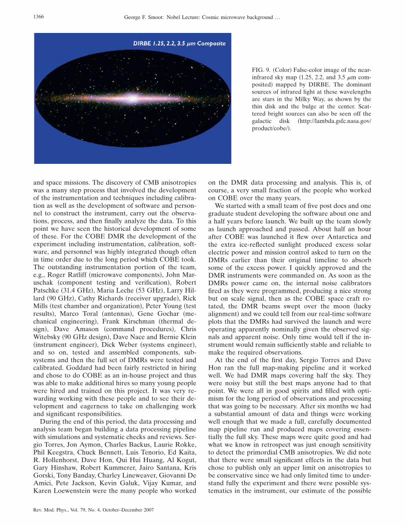
and space missions. The discovery of CMB anisotropieswas a many step process that involved the developmentof the instrumentation and techniques including calibra-tion as well as the development of software and person-nel to construct the instrument, carry out the observa-tions, process, and then finally analyze the data. To thispoint we have seen the historical development of someof these. For the COBE DMR the development of theexperiment including instrumentation, calibration, soft-ware, and personnel was highly integrated though oftenin time order due to the long period which COBE took.The outstanding instrumentation portion of the team,e.g., Roger Ratliff �microwave components�, John Mar-uschak �component testing and verification�, RobertPatschke �31.4 GHz�, Maria Leche �53 GHz�, Larry Hil-lard �90 GHz�, Cathy Richards �receiver upgrade�, RickMills �test chamber and organization�, Peter Young �testresults�, Marco Toral �antennas�, Gene Gochar �me-chanical engineering�, Frank Kirschman �thermal de-sign�, Dave Amason �command procedures�, ChrisWitebsky �90 GHz design�, Dave Nace and Bernie Klein�instrument engineer�, Dick Weber �systems engineer�,and so on, tested and assembled components, sub-systems and then the full set of DMRs were tested andcalibrated. Goddard had been fairly restricted in hiringand chose to do COBE as an in-house project and thuswas able to make additional hires so many young peoplewere hired and trained on this project. It was very re-warding working with these people and to see their de-velopment and eagerness to take on challenging workand significant responsibilities.

During the end of this period, the data processing andanalysis team began building a data processing pipelinewith simulations and systematic checks and reviews. Ser-gio Torres, Jon Aymon, Charles Backus, Laurie Rokke,Phil Keegstra, Chuck Bennett, Luis Tenorio, Ed Kaita,R. Hollenhorst, Dave Hon, Qui Hui Huang, Al Kogut,Gary Hinshaw, Robert Kummerer, Jairo Santana, KrisGorski, Tony Banday, Charley Lineweaver, Giovanni DeAmici, Pete Jackson, Kevin Galuk, Vijay Kumar, andKaren Loewenstein were the many people who worked

on the DMR data processing and analysis. This is, ofcourse, a very small fraction of the people who workedon COBE over the many years.

We started with a small team of five post docs and onegraduate student developing the software about one anda half years before launch. We built up the team slowlyas launch approached and passed. About half an hourafter COBE was launched it flew over Antarctica andthe extra ice-reflected sunlight produced excess solarelectric power and mission control asked to turn on theDMRs earlier than their original timeline to absorbsome of the excess power. I quickly approved and theDMR instruments were commanded on. As soon as theDMRs power came on, the internal noise calibratorsfired as they were programmed, producing a nice strongbut on scale signal, then as the COBE space craft ro-tated, the DMR beams swept over the moon �luckyalignment� and we could tell from our real-time softwareplots that the DMRs had survived the launch and wereoperating apparently nominally given the observed sig-nals and apparent noise. Only time would tell if the in-strument would remain sufficiently stable and reliable tomake the required observations.

At the end of the first day, Sergio Torres and DaveHon ran the full map-making pipeline and it workedwell. We had DMR maps covering half the sky. Theywere noisy but still the best maps anyone had to thatpoint. We were all in good spirits and filled with opti-mism for the long period of observations and processingthat was going to be necessary. After six months we hada substantial amount of data and things were workingwell enough that we made a full, carefully documentedmap pipeline run and produced maps covering essen-tially the full sky. These maps were quite good and hadwhat we know in retrospect was just enough sensitivityto detect the primordial CMB anisotropies. We did notethat there were small significant effects in the data butchose to publish only an upper limit on anisotropies tobe conservative since we had only limited time to under-stand fully the experiment and there were possible sys-tematics in the instrument, our estimate of the possible

FIG. 9. �Color� False-color image of the near-infrared sky map �1.25, 2.2, and 3.5 �m com-posited� mapped by DIRBE. The dominantsources of infrared light at these wavelengthsare stars in the Milky Way, as shown by thethin disk and the bulge at the center. Scat-tered bright sources can also be seen off thegalactic disk �http://lambda.gsfc.nasa.gov/product/cobe/�.



astrophysical foregrounds, or in the data processing andanalysis. We knew that we could make significant im-provements in the processing of the data and correct forsmall residual effects. We wanted also to do sensitivitystudies to ensure that we understood the experimentwell.

During my training as a young scientist, my mentors,including Dave Frisch, Luis Alvarez, and their col-leagues, repeatedly emphasized the importance of main-taining high scientific standards, both in choosing goodprojects and in executing them well. I heard of how im-portant it was in this kind of experiment to set up sys-tems and approaches so that one does not mislead one-self and assume that one has things right. Often even themost careful person lets down their vigilance when theresults are coming out as expected and pays more atten-tion when the result is different or unexpected. This issimply human nature and one must be careful not to fallin this trap. There was a famous paper showing the mea-surements of the speed of light with error estimates overtime. It systematically changes with time but almost al-ways within the estimated errors even though over manyexperiments, it changes by many standard deviations.This was unequivocal proof of this tendency and thusthe need to be rigorous and systematic regardless of theresult one was obtaining. One should work until confi-dent in how well one has done before looking at theresult and start believing in it. In many fields it is essen-tial procedure to do the experiment in a double-blindmethod so as to guard against this very expectation ef-fect.

So as soon as we had revamped and retested our dataprocessing and map-making pipeline, we carefully vali-dated it and then processed the full first-year data set.When the maps were made, there were clearly some re-sidual signals above the noise. A sure-fire indicator wasthat when we made maps at each DMR frequency �31.4,53, and 90 GHz� to get the best sensitivity we co-addedthe data from each of the two �A and B� channels ateach frequency. However, we could also difference theA and B maps which should subtract any sky signal andleave only the independent instrumental noise. The vari-ances and the smoothed AB maps looked significantlydifferent from the A-B maps. The A-B maps were con-sistent with what was expected from the simple Gauss-ian fluctuations of the receiver white noise. The questionwas: Were these extra signals from the CMB, from as-trophysical sources, from the instrument and experimen-tal procedures, or from the data processing? At one ofour COBE science team meetings I reported to the fullScience Working Group �SWG� that we saw some ef-fects but that it was too soon to be sure that it was notsome artifact. I set the goal for the DMR analysis teamof systematically going through all our steps and pro-cesses to show that we had each thing accounted forproperly since in this kind of experiment one attributesto the CMB everything that is not attributed to anythingelse. We set up a plan and schedule to work througheverything systematically and have each study confirmedand checked. The team fell into hard focused work on

this program not jumping right to the conclusion thatthis was CMB anisotropy but assuming that this was thecorrect approach. About six months �August 1991� intothis, Ned Wright turned part of his attention to theDMR and noted that the one-year DMR maps had fluc-tuations in them consistent with the cold dark matter�CDM� cosmological model. This did not deflect theDMR team much as they were still trying to get donethe projects set for them by their deadlines. In October,Ned Wright did another bit of processing of the one-yearmaps with software he wrote and concluded that thedata fit a Harrison-Zel’dovich spectrum with a corre-sponding quadrupole amplitude of about 15 �K. Wefound about 30 �K in the DMR official software. Nedwas now excited about the DMR potential results andwanted to bring it up at the next science team meeting.We agreed to have it at a more private special eveningmeeting after dinner at Al and Nancy Boggess’s house asit would be a sensitive issue. The WG �as I argued�thought it appropriate to be conservative, educate all themembers of the team on the status and reliability of theresults, and have the DMR team prepare and present tothe full science team a review of all portions of theDMR experiment. This review was set for the end of theyear 1991.

This extra attention from the SWG began to affect theDMR analysis team. They did not want to miss out onthe discovery and especially the fun and excitement ofthe science analysis and the cosmological implications. Itried to have no one work on science analysis papers�myself included� until the checks were done. This wasfor the very point of ensuring that we had done a jobthat we were very confident was as good as possible. Iworked hard to keep them on track and careful aboutgetting the correct results and went so far as to offer twofree tickets anywhere in the world to any one that couldfind an effect from anything �other than the CMB� whatwould explain a significant portion of what we were see-ing. We divided into specialists in the areas of instru-mental errors �led by the outstandingly able Alan Kogutwho had to deal with very many potential issues�, galac-tic foregrounds �Chuck Bennett and Gary Hinshaw�,software �Sergio Torres for the DMR official code,George Smoot and my graduate students Luis Tenorioand Charley Lineweaver creating independent code andtests, and Ned Wright with his own map processing soft-ware�, and so forth. David Wilkinson was a particularlydetermined skeptic keeping everyone on their toes.

We held the review just after New Year’s and pre-sented all the tests, checks, calibrations, and results in aday long review with extra material to the full DMR andSWG. There were a few things left to follow up but withthem underway, we turned to analyzing the maps fortheir scientific results. There are a number of interestingthings here including the low quadrupole and so forthbut the most important issue was following a rigorousprocedure. This was evident to me when we had the lastSWG meeting to review the results and papers and dis-cuss going public. At that meeting we also heard fromthe MIT-Princeton team with a balloon-borne bolometer



experiment whose data seemed to support the DMR re-sults though were not as strong as the DMR. Thatseemed consistent but not conclusive. Then Phil Lubingot up and argued against going public stating that hisgroup’s data from their South Pole experiment was in-consistent and had a lower upper limit than the DMRresults. This caused concern among some of the SWGbut I found myself confidently arguing for going forwardand publishing. I felt that the DMR team had doneabout as good a job as one could and were very likely tobe correct.

On April 23, 1992, the COBE team announced thehistorical discovery of the anisotropies of cosmic micro-wave background radiation with characteristic aniso-tropy �T /T�10−5 or �T�30 �K on angular scaleslarger than �7° at the annual meeting of AmericanPhysical Society in Washington, D.C. �Smoot et al.,1992�. The CMB anisotropy provides very rich informa-tion on the early universe, allowing the calculation ofcosmological parameters and discrimination of variousdetailed models of the big bang. The anisotropy mapproduced by the COBE DMR is composed of 6144 pix-els each 2.6° 2.6°. This can be compared to the size ofa patch of sky subtended by light that had been travelingsince the beginning of the universe, about 1°. That is, theperturbations detected by DMR are directly from theprimordial state set at the beginning. After four years ofmeasurements by the COBE DMR, the typical signal-to-noise ratio in a 10° smoothed frequency-averagedmap rose to �2, so the anisotropy could be seen by eye.The DMR found the CMB thermodynamic temperatureof T0=2.725±0.020 K which was well consistent with theresult of COBE FIRAS. If we subtract this temperaturefrom the map and change the scale by a factor of 1000,the CMB dipole looms out of the uniform backgroundwith amplitude 3.358±0.024 mK toward the galactic co-ordinates �lG ,bG�= �264.31±0.16°, 48.05° ±0.10°� recon-firming the discovery of U2 flight experiments. Whenthe scale is increased to 100 000, higher multipoles �l�2� can be seen. Figure 10 shows these features at theseincreasing scale factors. The quadrupole amplitude wasestimated between 4 and 28 �K. The analysis of multi-poles with l�2 showed that the fluctuations are consis-tent with scale invariant �an n=1 power-law� fluctuationspectrum as predicted by models of the inflationary bigbang �Fig. 11�. Another important test for the inflation-ary big bang theory is the Gaussian distribution of theprimordial temperature fluctuations. Our COBE DMRdata found no evidence for deviations from a Gaussiandistribution �Smoot et al., 1994� as have all the experi-ments that have followed thus far.

II. FORGING THE STANDARD MODEL OF COSMOLOGY:�CDM

A. The suborbital CMB experiments

The CMB anisotropy is the most important cosmo-logical observable to date, so many more ground-basedand balloon-borne CMB experiments followed the

COBE mission in 1990s �Smoot et al., 1997�. While someexperiments focused on large angular scales at fre-quency bands not used in the COBE DMR, most of theprojects worked on the smaller angular scales whichwere not explored by the COBE DMR. These small an-gular scale experiments put very tight constraints on cos-mological models. Results from some representative ex-periments on the angular power spectrum are presentedin Fig. 12. Supernovae observations startled the cosmol-ogy community with the discovery of accelerated expan-sion of space �Riess et al., 1998; Perlmutter et al., 1999�.This brought back the cosmological constant to the Ein-stein equations, introduced originally with different mo-tivation and then discarded soon after. Observationsother than the CMB experiments including galaxy sur-veys have provided valuable information and allowedcross checks with the results from the CMB experi-ments. Some recent results of suborbital experiments

FIG. 10. �Color� The breakdown of the CMB sky map pro-duced by COBE DMR �http://lambda.gsfc.nasa.gov/product/cobe/�, monopole �top�, dipole �middle�, and multipole �bot-tom�. At T�3 K level �top�, we have uniform radiation fromevery direction. When the sensitivity is changed to �mK level,the dipole pattern shows up, which is due to the peculiar mo-tion of our solar system relative to the CMB rest frame. As thescale is refined to �T�10 �K, after removal of the dipole, themultipole features of anisotropy become evident. These verytiny fluctuations give us information about the early universe.



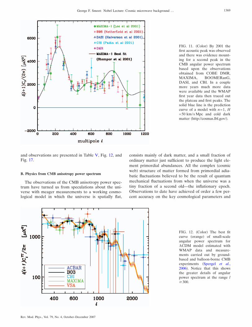
and observations are presented in Table V, Fig. 12, andFig. 17.

B. Physics from CMB anisotropy power spectrum

The observations of the CMB anisotropy power spec-trum have turned us from speculations about the uni-verse with meager measurements to a working cosmo-logical model in which the universe is spatially flat,

consists mainly of dark matter, and a small fraction ofordinary matter just sufficient to produce the light ele-ment primordial abundances. All the complex �cosmicweb� structure of matter formed from primordial adia-batic fluctuations believed to be the result of quantummechanical fluctuations from when the universe was atiny fraction of a second old—the inflationary epoch.Observations to date have achieved of order a few per-cent accuracy on the key cosmological parameters and

FIG. 11. �Color� By 2001 thefirst acoustic peak was observedand there was evidence mount-ing for a second peak in theCMB angular power spectrumbased upon the observationsobtained from COBE DMR,MAXIMA, BOOMERanG,DASI, and CBI. In a couplemore years much more datawere available and the WMAPfirst year data then traced outthe plateau and first peaks. Thesolid blue line is the predictioncurve of a model with n=1, H=50 km/s Mpc and cold darkmatter �http://cosmas.lbl.gov/�.

FIG. 12. �Color� The best fitcurve �orange� of small-scaleangular power spectrum for�CDM model estimated withWMAP data and measure-ments carried out by ground-based and balloon-borne CMBexperiments �Spergel et al.,2006�. Notice that this showsthe greater details of angularpower spectrum at the range l�300.



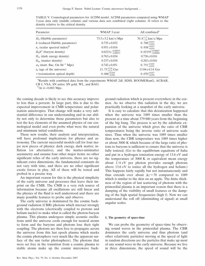
the coming decade is likely to see this accuracy improveto less than a percent. In large part, this is due to theexpected improvement in CMB temperature and polar-ization anisotropies. That change will make a very sub-stantial difference in our understanding and in our abil-ity not only to determine those parameters but also totest the key elements of the assumed physics of our cos-mological model and even probe what were the naturaland minimum initial conditions.

These new results, their analysis and interpretation,will have profound implications for physics and as-tronomy. The current successful models call for four ma-jor new pieces of physics: dark energy, dark matter, in-flation �or alternative�, and the matter-antimatterasymmetry and assume four other major items: no othersignificant relics of the early universe, there are no sig-nificant extra dimensions, the fundamental constants donot vary with time, and there are no other significantexotic forces in play. All of these will be tested andprobed in a precise way.

An important reason for this is the physical simplicityof the early universe and processes that leave their im-print on the CMB. The CMB is a very rich source ofinformation because all oscillations are still linear andthe physics of the fluid is well understood and there aremany possible features to probe and observe.

The early universe is dominated by the cosmic back-ground radiation �CBR� photons which interact stronglywith the electrons �electrically coupled to protons andhelium nuclei� to make what is called the photon-baryonplasma. This plasma undergoes simple acoustic oscilla-tions until the universe cools enough for neutral atomsto form and the baryons and photons lose their tightcoupling. The photons are then free to propagate acrossthe universe from this last epoch plasma which marksthe cosmic photosphere very much like the apparent sur-face of the sun �solar photosphere�. The photons thatwere set free in the transition from a cosmic plasma tostable atoms make up the cosmic microwave back-

ground radiation which is present everywhere in the cos-mos. As we observe this radiation in the sky, we arepractically looking at a snapshot of the early universe.

It is easy to calculate that this deionization happenedwhen the universe was 1089 times smaller than thepresent at a time about 379 000 years from the beginningof the big bang. The process is set by the adiabatic ex-pansion of the universe which gives the ratio of CBRtemperatures being the inverse ratio of universe scalesizes. Thus when the universe was 1089 times smallerthan now, the CBR temperature was 1089 times higheror about 3000 K which because of the large ratio of pho-tons to baryons is sufficient to ensure that the universe isfully ionized. �Go to the equilibrium equations of Sahaand put in a hydrogen ionization energy of 13.6 eV andthe temperature of 3000 K or equivalent mean energyabout 1/4 eV per photon provides enough photonsabove 13.6 eV to ionize all the hydrogen and helium.�This happens fairly rapidly but not instantaneously andthus extends over about �z�70 compared to 1089which is similar to the skin on an apple. The finite thick-ness of the region of last scattering of photons with theprimordial plasma is an important reason that there is adamping of the visibility of small features or the damp-ing of the high spatial frequencies �high l�. Now we canunderstand the roll off �diminishing of signal� at smallangular scales.

1. The geometry of space-time

We can probe the geometry of space-time by observ-ing sound waves in the primordial plasma. The CBRdominates the early universe and thus photons �andother relativistic particles� moving at the speed of lightin random directions are the particles that make up mostof any sound wave in the early universe. Because we livein three dimensions, the speed of sound will be the

TABLE V. Cosmological parameters for �CDM model. �CDM parameters computed using WMAP3-year data only �middle column� and various data sets combined �right column�. � refers to thedensity relative to the critical density.

Parameter WMAP 3-year All combineda

H0 �Hubble parameter� 73.5±3.2 km/s /Mpc 70.8−1.6+1.5 km/s /Mpc

h �reduced Hubble parameter� 0.735±0.032 0.708−0.016+0.015

ns �scalar spectral index�b 0.951±0.016 0.938−0.014+0.015

�bh2 �baryon density� 0.0223±−0.00073+0.00075 0 .02193−0.00068

+0.00067

�� dark energy density� 0.763±0.034 0.738±0.016�m �matter density� 0.237±0.034 0.262±0.0168 �matt. fluc. On 8h−1 Mpc� 0.742±0.051 0.751−0.031

+0.032

t0 �age of the universe� 13.73−0.15+0.16 Gyr 13.84±0.14 Gyr

� �reionization optical depth� 0.088−0.030+0.029 0 .070−0.028

+0.027

aResults with combined data from the experiments WMAP, 2df, SDSS, BOOMERanG, ACBAR,CB I, VSA, SN astier, SN gold, WL, and BAO.

bAt k=0.002/Mpc.



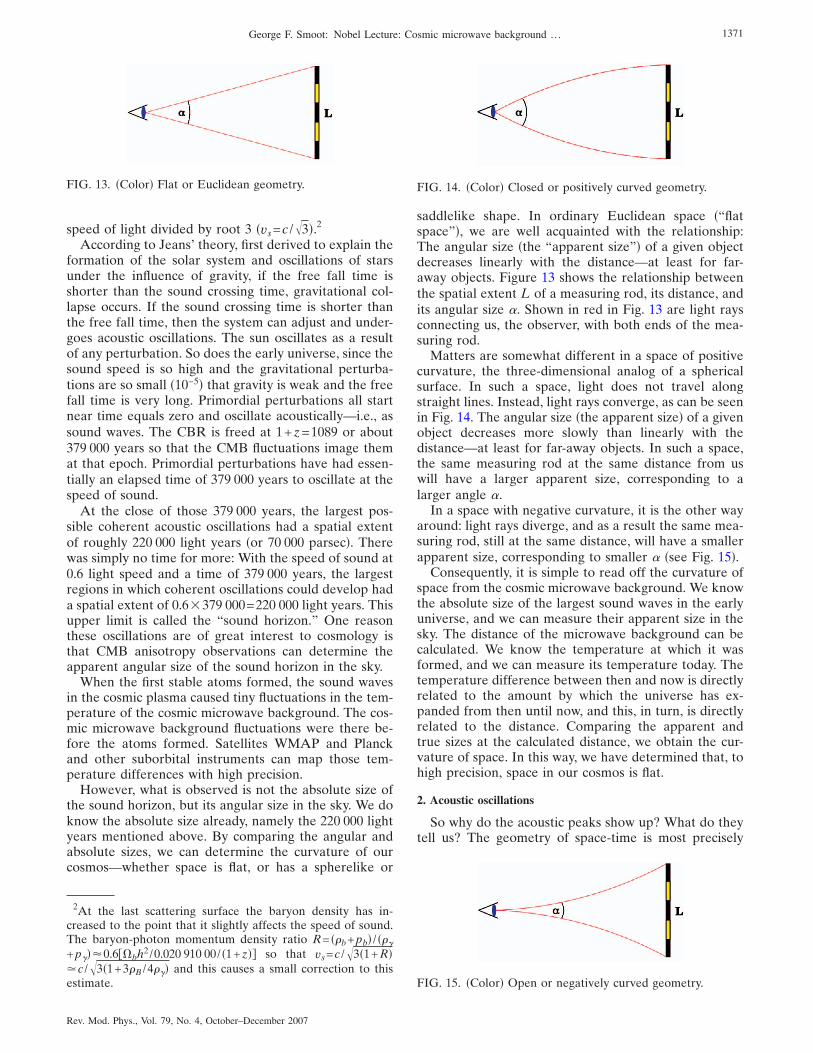
speed of light divided by root 3 �vs=c /3�.2

According to Jeans’ theory, first derived to explain theformation of the solar system and oscillations of starsunder the influence of gravity, if the free fall time isshorter than the sound crossing time, gravitational col-lapse occurs. If the sound crossing time is shorter thanthe free fall time, then the system can adjust and under-goes acoustic oscillations. The sun oscillates as a resultof any perturbation. So does the early universe, since thesound speed is so high and the gravitational perturba-tions are so small �10−5� that gravity is weak and the freefall time is very long. Primordial perturbations all startnear time equals zero and oscillate acoustically—i.e., assound waves. The CBR is freed at 1+z=1089 or about379 000 years so that the CMB fluctuations image themat that epoch. Primordial perturbations have had essen-tially an elapsed time of 379 000 years to oscillate at thespeed of sound.

At the close of those 379 000 years, the largest pos-sible coherent acoustic oscillations had a spatial extentof roughly 220 000 light years �or 70 000 parsec�. Therewas simply no time for more: With the speed of sound at0.6 light speed and a time of 379 000 years, the largestregions in which coherent oscillations could develop hada spatial extent of 0.6 379 000=220 000 light years. Thisupper limit is called the “sound horizon.” One reasonthese oscillations are of great interest to cosmology isthat CMB anisotropy observations can determine theapparent angular size of the sound horizon in the sky.

When the first stable atoms formed, the sound wavesin the cosmic plasma caused tiny fluctuations in the tem-perature of the cosmic microwave background. The cos-mic microwave background fluctuations were there be-fore the atoms formed. Satellites WMAP and Planckand other suborbital instruments can map those tem-perature differences with high precision.

However, what is observed is not the absolute size ofthe sound horizon, but its angular size in the sky. We doknow the absolute size already, namely the 220 000 lightyears mentioned above. By comparing the angular andabsolute sizes, we can determine the curvature of ourcosmos—whether space is flat, or has a spherelike or

saddlelike shape. In ordinary Euclidean space �“flatspace”�, we are well acquainted with the relationship:The angular size �the “apparent size”� of a given objectdecreases linearly with the distance—at least for far-away objects. Figure 13 shows the relationship betweenthe spatial extent L of a measuring rod, its distance, andits angular size �. Shown in red in Fig. 13 are light raysconnecting us, the observer, with both ends of the mea-suring rod.

Matters are somewhat different in a space of positivecurvature, the three-dimensional analog of a sphericalsurface. In such a space, light does not travel alongstraight lines. Instead, light rays converge, as can be seenin Fig. 14. The angular size �the apparent size� of a givenobject decreases more slowly than linearly with thedistance—at least for far-away objects. In such a space,the same measuring rod at the same distance from uswill have a larger apparent size, corresponding to alarger angle �.

In a space with negative curvature, it is the other wayaround: light rays diverge, and as a result the same mea-suring rod, still at the same distance, will have a smallerapparent size, corresponding to smaller � �see Fig. 15�.

Consequently, it is simple to read off the curvature ofspace from the cosmic microwave background. We knowthe absolute size of the largest sound waves in the earlyuniverse, and we can measure their apparent size in thesky. The distance of the microwave background can becalculated. We know the temperature at which it wasformed, and we can measure its temperature today. Thetemperature difference between then and now is directlyrelated to the amount by which the universe has ex-panded from then until now, and this, in turn, is directlyrelated to the distance. Comparing the apparent andtrue sizes at the calculated distance, we obtain the cur-vature of space. In this way, we have determined that, tohigh precision, space in our cosmos is flat.

2. Acoustic oscillations

So why do the acoustic peaks show up? What do theytell us? The geometry of space-time is most precisely

2At the last scattering surface the baryon density has in-creased to the point that it slightly affects the speed of sound.The baryon-photon momentum density ratio R= ��b+pb� / ��

+p��0.6��bh2 /0.020 910 00/ �1+z�� so that vs=c /3�1+R��c /3�1+3�B /4�� and this causes a small correction to thisestimate.

FIG. 13. �Color� Flat or Euclidean geometry. FIG. 14. �Color� Closed or positively curved geometry.

FIG. 15. �Color� Open or negatively curved geometry.



determined by measuring the angular scale of the firstacoustic oscillation peak in the angular power spectrum.With observations of several peaks we are able to tiedown several parameters and determine the geometry ofspace-time even more precisely. How can we understandthe plateau and the acoustic peaks?

That again is conceptually simple. If a physical systemis hit by a spike of short duration—the extreme versionis a Dirac delta function, i.e., an impulse of zero timeduration—then all possible oscillation modes are excitedequally on average but stochastically. This would beequivalent for the early universe of equal power or iden-tical rms perturbation amplitudes into all plane wave forflat space-time or appropriate modes. So, if we choosethe correct plotting of the angular power spectrum, theinitial perturbations or excitation would be basically in-dependent of scale and particularly angular frequency.The finite thickness of last scattering will damp out thehigh angular frequencies. Another effect which is leak-age of photons out of high frequency perturbations be-cause of minor edge effects adds to this effect. Becauseof the geometry of space-time and the contents of theuniverse, this otherwise nearly scale invariant powerspectrum has a set of acoustic peaks at a fundamentalangular frequency and its harmonics. These are reallythree-dimensional perturbations that are then mani-fested upon the apparently spherical sky.

On the largest angular scales, e.g., those first observedby the COBE DMR, we observe what are the basicallyinitial conditions. These scales are so large that evenmoving at the full speed of sound �c /3� the change issmall compared to the size of the structure and elementsthat large have only undergone a very small fraction ofan oscillation from the beginning until the last scatteringsurface. Perturbations that are much larger than thesound horizon remain little changed and will show up inthe power spectrum as simply the low angular frequency�large angular scale� plateau that reflect the primordialperturbations. Without the acoustic oscillations, the an-gular power spectrum would remain flat until the highangular frequency �small physical scales� damping cuts itoff.

Why is there a well-defined first peak, if all scales aresimply oscillating and there is little damping on thelarger scales?

However, when one reaches the scale of about 220 000light years at the surface and time of last scattering, theoscillation has had time to just fully compress. Compres-sion makes that region hotter and that is what shows upin the snap shot provided by the CMB.

At half that size an acoustic oscillation has time tocompress and then expand and reach maximum rarefac-tion. It would appear to be cooler than the average. Inan angular power spectrum this would appear as the sec-ond peak, since taking the power rectifies �squares� thevariation which was to cooler.

At one-third that size the acoustic oscillation has timeto compress, rarify, and reach maximum compressionagain. This is the source of the third acoustic. And so onfor higher spatial frequency peaks. It will appear warmer

than the average. At 3/4 that size the oscillation hascompressed and then expanded back to the startingplace for no contrast to the average. Thus measuring themean square fluctuations on each scale or the powerspectrum, one would anticipate peaks at the sound hori-zon, half the sound horizon, one-third the sound hori-zon, etc., and then nulls midway in between. However,there is an additional effect from the motion of theoscillations—at the halfway points the sound wave ismoving with maximum speed and the Doppler effectproduces a small secondary peak exactly out of phasewith the compression and rarefaction. These somewhatfill in between the acoustic peaks so that there is not aprecise null.

The key points are that �i� compressed fluid is hotter,�ii� oscillation frequency scales inversely with size, �iii�oscillations stop at last scattering, �iv� nulls of oscilla-tions are when the Doppler effect is maximal from themotion of oscillation, and �v� fluctuations are imprintedon CMB at the last scattering surface.

All these effects are readily calculable as they dependonly on the geometry and the speed of sound. There aresmall corrections for the speed of sound near last scat-tering due to the baryon loading �baryons are relativelymore important as the CMB is cooled by the expansionof the universe� and also the effect of the dark matterand even a small correction for dark energy. One findsthat the height of the first peak is proportional to thetotal matter content of the universe while the second�rarefaction� peak is set more by the baryon content andso on. As a result, by carefully fitting to the amplitudesand l values, one can precisely constrain the physicaldensity of baryons and dark matter as well as the geom-etry of space-time.

The first acoustic peak occurs at l�200 or about 0.9°angular scale for a flat universe. The early observationsquickly confirmed this value indicative of a universenear flat. Now observations are getting sufficiently pre-cise that one must take into account the small correc-tions that come from the possible variation of the con-tents of the universe. One must take into account thatthe photon-baryon fluid is not purely photon dominatedat the last scattering surface. Baryons add to the mass ofthe photon-baryon plasma without adding pressure.Also the universe is not exactly matter dominated andthere is some dark energy content. The dark energy con-tent comes to dominate in later epochs and changes thedistance to the last scattering surface somewhat and thuschanges the apparent angles on the sky a small amount.All of these effects are small but are important at thepercent to few percent level. By far the most dominantfactor is the geometry of the universe and via generalrelativity the total energy content of the universe is veryclose to the critical value. In current models this means�total=�m+��=1.02±0.02.

3. The dark matter and the baryon content of the universe

By the epoch of last scattering the energy density indark matter gets to be larger than the energy density in



photons. As a result, the inertia and gravitational poten-tial of matter is the source of the restoring force �grav-ity� for the acoustic oscillations and thus affects the am-plitude of the oscillations directly. Thus the height of theacoustic peaks is proportional to the total mass densitywhich is primarily dark matter. By measuring the heightof the peaks, particularly the first peak, the physical den-sity of matter �mh2 is well determined.

Baryons �or ordinary matter� load down the photon-baryon plasma and add inertial �and gravitational� massto the oscillating system. The effect on the acousticpeaks is easy to understand. If one adds mass to a springand lets it fall in the gravitational field, with more massloading the spring, it falls further before pulled back bythe spring. Then it rebounds to the same position itstarted from. That is the maximum compression in-creases but the rarefaction is unchanged.

Since the odd numbered �first, third, fifth, etc.� acous-tic peaks are associated with how much the plasma com-presses �falls into the gravitational potential wells�, theyare enhanced by an increase in the amount of baryons inthe universe. The even numbered peaks �second, fourth,sixth� are associated with how far the plasma rarefies�rebounds in the gravitational field�. The addition ofbaryons enhances the odd peaks over the even peaks.Added baryons make the first acoustic peak much largerthan the second. The more baryons the more the secondpeak is relatively suppressed.

If baryons contribute a negligible amount of mass tothe plasma, the CMB temperature at the bottom of thepotential well oscillates symmetrically around zero. Withmore baryons in the system, the plasma is loaded down.The plasma compresses further inside the potential wellbefore pressure can reverse the motion. The oscillationis now asymmetric in that the extrema that representcompressions inside potential wells are increased overthose that represent rarefactions. The power spectrumdoes not care about the sign and so takes the absolutevalue of the temperature fluctuation. Now we see thatthe first and third peaks are enhanced over the secondpeak. When we do the full calculation of the power spec-trum, the basic physics of a mass on the spring appearsas advertised. The odd numbered acoustic peaks in thepower spectrum are enhanced in amplitude over theeven numbered ones as we increase the baryon densityof the universe.

There are second order effects. Since adding mass to aspring slows the oscillation down, adding baryons to theplasma decreases the frequency of the oscillations push-ing the position of the peaks to slightly higher multipolesl. �More bayons means slightly slower sound speed so agiven number of oscillation cycles must take place over asmall size; �s↓ ⇒ l↑.� Baryons also affect how soundwaves damp, which affects how the spectrum falls off athigh l. The many ways that baryons show up in the an-gular power spectrum provides many independentchecks on the baryon density of the universe. Thebaryon density is a quantity that the CMB can measureto exquisite precision. The CMB observations agreewith big bang nucleosynthesis �BBN� at about 4.4±0.4%

of critical density. The BBN estimate comes fromnuclear physics and conditions in the first few minutes ofthe big bang. The CMB acoustic peaks ratio comes fromatomic physics at 380 000 years after the big bang. As aconsequence there has been no significant change in thebaryon-photon ratio from an energy scale of an MeV toan eV and probably to now with an energy scale of1/4000 eV which is a substantial portion of the expan-sion history of the universe.

4. Other cosmological parameters including dark energy,equation of state

The CMB anisotropies are sensitive in varying de-grees to a number of other cosmological quantities in-cluding the dark energy density, its equation of state, theage of the universe, the optical depth to the re-ionization of the universe, and the slight tilt of the pri-mordial perturbation spectrum. For some of these obser-vations of the CMB the angular power spectrum turnout to be extremely sensitive for some others there aredegeneracies or near degeneracies that require the CMBobservations to be combined with other cosmologicalobservations to get a truly accurate result. Needless tosay, the CMB anisotropies do provide a substantialamount of information. In principle, measuring thepower spectrum multipoles provides up to 3000 indepen-dent numbers; while we believe that our standard modelof cosmology can be well described by less than 20 pa-rameters. Thus we have substantial redundancy goingfrom millions of pixels in our maps, by assuming rota-tional invariance down to about 3000 numbers in theangular power spectrum and then by cosmologicalmodel fitting down to a couple of dozen parameters.

C. Wilkinson microwave anisotropy probe

The Wilkinson microwave anisotropy probe �WMAP�mission was the second, more extensive satellite-borneCMB project also by NASA, which followed the COBE�see Fig. 16�. The skymap data taken by WMAP have 45times the sensitivity and 33 times the angular resolutionof the COBE DMR mission. WMAP used five separatefrequency bands from 23 to 94 GHz. The goal ofWMAP was to map the relative CMB temperature overthe full sky with an angular resolution �0.3°, a sensitiv-ity of 20 �K per 0.3° 0.3° square pixel, with systematicartifacts limited to 5 �K per pixel. In February 2003, theWMAP first-year data and results were released andthree-year data were released in March 2006�http:map.gsfc.nasa.gov/�. The results strongly supportthe inflationary big bang models. WMAP also set tightconstraints on the cosmological models, among whichthe �CDM model �nearly flat universe with dark energy�70%, cold dark matter �25%, baryonic matter �5%�fits best with WMAP along with various independentexperiments �see Table V and Fig. 17�.



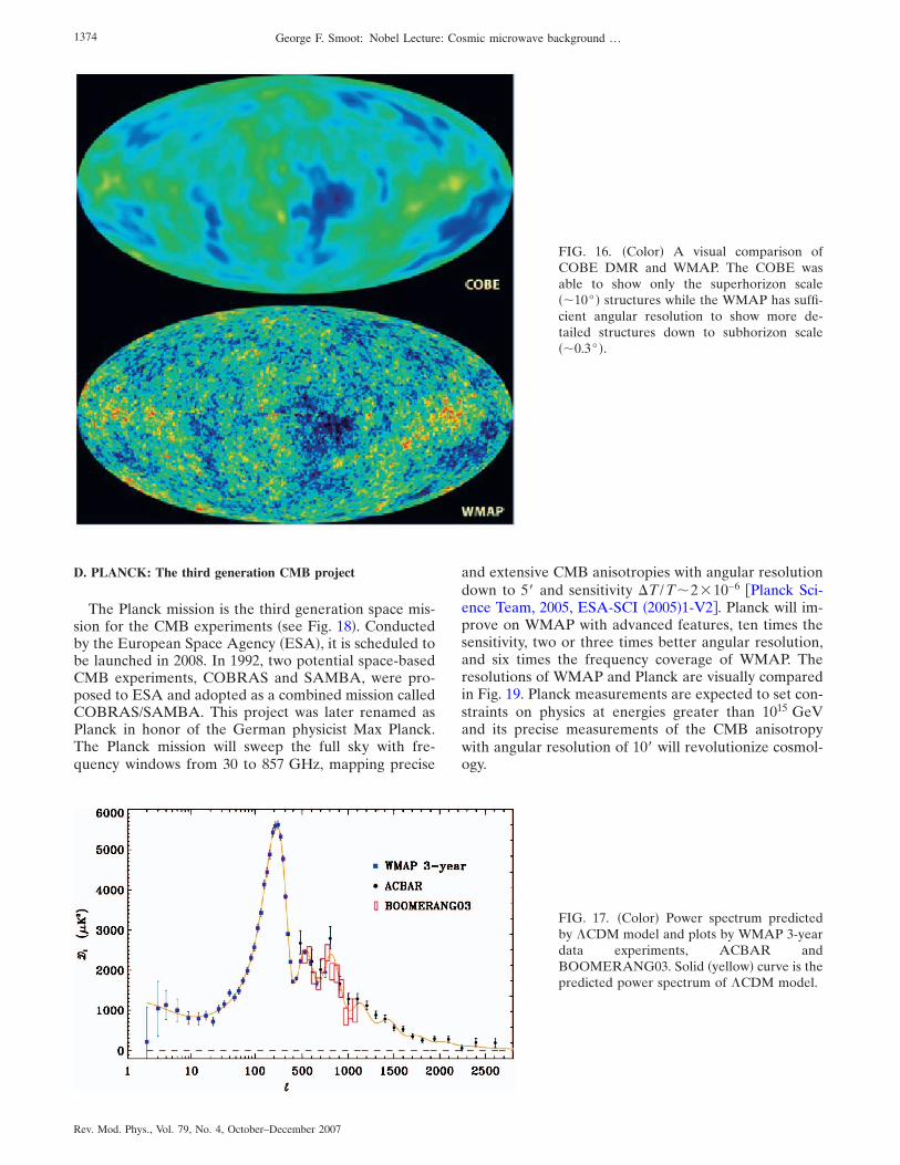
D. PLANCK: The third generation CMB project

The Planck mission is the third generation space mis-sion for the CMB experiments �see Fig. 18�. Conductedby the European Space Agency �ESA�, it is scheduled tobe launched in 2008. In 1992, two potential space-basedCMB experiments, COBRAS and SAMBA, were pro-posed to ESA and adopted as a combined mission calledCOBRAS/SAMBA. This project was later renamed asPlanck in honor of the German physicist Max Planck.The Planck mission will sweep the full sky with fre-quency windows from 30 to 857 GHz, mapping precise

and extensive CMB anisotropies with angular resolutiondown to 5� and sensitivity �T /T�2 10−6 �Planck Sci-ence Team, 2005, ESA-SCI �2005�1-V2�. Planck will im-prove on WMAP with advanced features, ten times thesensitivity, two or three times better angular resolution,and six times the frequency coverage of WMAP. Theresolutions of WMAP and Planck are visually comparedin Fig. 19. Planck measurements are expected to set con-straints on physics at energies greater than 1015 GeVand its precise measurements of the CMB anisotropywith angular resolution of 10� will revolutionize cosmol-ogy.

FIG. 16. �Color� A visual comparison ofCOBE DMR and WMAP. The COBE wasable to show only the superhorizon scale��10° � structures while the WMAP has suffi-cient angular resolution to show more de-tailed structures down to subhorizon scale��0.3° �.

FIG. 17. �Color� Power spectrum predictedby �CDM model and plots by WMAP 3-yeardata experiments, ACBAR andBOOMERANG03. Solid �yellow� curve is thepredicted power spectrum of �CDM model.



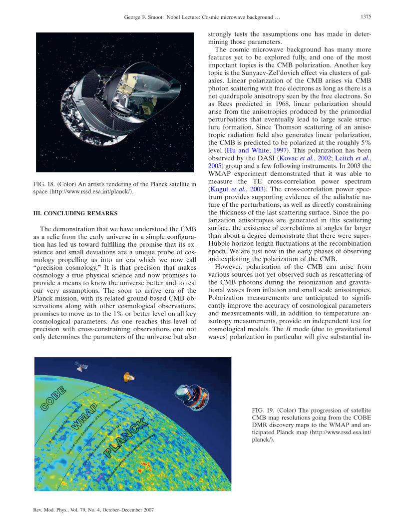
III. CONCLUDING REMARKS

The demonstration that we have understood the CMBas a relic from the early universe in a simple configura-tion has led us toward fulfilling the promise that its ex-istence and small deviations are a unique probe of cos-mology propelling us into an era which we now call“precision cosmology.” It is that precision that makescosmology a true physical science and now promises toprovide a means to know the universe better and to testour very assumptions. The soon to arrive era of thePlanck mission, with its related ground-based CMB ob-servations along with other cosmological observations,promises to move us to the 1% or better level on all keycosmological parameters. As one reaches this level ofprecision with cross-constraining observations one notonly determines the parameters of the universe but also

strongly tests the assumptions one has made in deter-mining those parameters.

The cosmic microwave background has many morefeatures yet to be explored fully, and one of the mostimportant topics is the CMB polarization. Another keytopic is the Sunyaev-Zel’dovich effect via clusters of gal-axies. Linear polarization of the CMB arises via CMBphoton scattering with free electrons as long as there is anet quadrupole anisotropy seen by the free electrons. Soas Rees predicted in 1968, linear polarization shouldarise from the anisotropies produced by the primordialperturbations that eventually lead to large scale struc-ture formation. Since Thomson scattering of an aniso-tropic radiation field also generates linear polarization,the CMB is predicted to be polarized at the roughly 5%level �Hu and White, 1997�. This polarization has beenobserved by the DASI �Kovac et al., 2002; Leitch et al.,2005� group and a few following instruments. In 2003 theWMAP experiment demonstrated that it was able tomeasure the TE cross-correlation power spectrum�Kogut et al., 2003�. The cross-correlation power spec-trum provides supporting evidence of the adiabatic na-ture of the perturbations, as well as directly constrainingthe thickness of the last scattering surface. Since the po-larization anisotropies are generated in this scatteringsurface, the existence of correlations at angles far largerthan about a degree demonstrate that there were super-Hubble horizon length fluctuations at the recombinationepoch. We are just now in the early phases of observingand exploiting the polarization of the CMB.

However, polarization of the CMB can arise fromvarious sources not yet observed such as rescattering ofthe CMB photons during the reionization and gravita-tional waves from inflation and small scale anisotropies.Polarization measurements are anticipated to signifi-cantly improve the accuracy of cosmological parametersand measurements will, in addition to temperature an-isotropy measurements, provide an independent test forcosmological models. The B mode �due to gravitationalwaves� polarization in particular will give substantial in-

FIG. 18. �Color� An artist’s rendering of the Planck satellite inspace �http://www.rssd.esa.int/planck/�.

FIG. 19. �Color� The progression of satelliteCMB map resolutions going from the COBEDMR discovery maps to the WMAP and an-ticipated Planck map �http://www.rssd.esa.int/planck/�.



formation on the energy scale of inflation. The CMB isalso a favored subject in which one can probe theorizedremnants of big bang inflation such as topological de-fects �http://cosmos.lbl.gov/� which are directly related tophysics in very early universe �T�1016 GeV�.

ACKNOWLEDGMENTS

I would like to thank and acknowledge the manypeople who contributed to this work, particularly mymany colleagues and co-workers over the years and par-ticularly the COBE team. The development of cosmol-ogy has been a significant intellectual achievement pow-ered by the work of very many scientists, engineers, andstaff over many decades. A number of slides and figuresthat I used in my Nobel Lecture were provided by oth-ers and many names were cut off; unfortunately, in therush of connecting my laptop, the wrong resolution wasused and the edges of the slides not projected. Amongthe many slides were those from Don Groom, Al Kogut,Wayne Hu, Ned Wright, WMAPSDSS, Max Tegmark,David Wilkinson, Julian Borrill, and others which werethere but not shown. I thank a number of colleagues,especially my graduate students and post docs for theirdiscussions and comments both at present and over themany years as well as for their great excitement andintellectual efforts on the various projects. EunhwaJeong and Bruce Grossan were directly helpful with thiswrite up. This work was supported by the Lawrence Ber-keley National Laboratory and the Department of Phys-ics at the University of California, Berkeley.

REFERENCES

Alpher, R. A., H. Bethe, and G. Gamow, 1948, “The origin ofchemical elements,” Phys. Rev. 73, 803–804.

Alpher, R. A., J. W. Follin, and R. C. Herman, 1953, “Physicalconditions in the initial stages of the expanding universe,”Phys. Rev. 92, 1347–1361.

Alpher, R. A., G. Gamow, and R. Herman, 1967, “Thermalcosmic radiation and the formation of protogalaxies,” Proc.Natl. Acad. Sci. U.S.A. 58, 2179–2186.

Alpher, R. A., and R. C. Herman, 1953, “The origin and abun-dance distribution of the elements,” Annu. Rev. Nucl. Sci. 2,1–40.

Alpher, R. A., and R. C. Herman, 1988, “Reflections on earlywork on ‘big bang’ cosmology,” Phys. Today 41 �8�, 24.

Alpher, R. A., and R. Herman, 1990, “Early work on ‘big-bang’ cosmology and the cosmic blackbody radiation,” Mod-ern Cosmology in Retrospect, edited by B. Bertotti, R. Balbi-not, and S. Bergia �Cambridge University Press, Cambridge,England�, p. 129.

Alpher, R. A., R. Herman, and G. A. Gamow, 1948, “Thermo-nuclear reactions in the expanding universe,” Phys. Rev. 74,1198.

Bahcall et al., 1973, Astrophys. J., Lett. Ed. 182, L95.Bensadoun et al., 1993, Astrophys. J. 409, 1.Bernstein et al., 1990, Astrophys. J. 362, 107.Bersanelli et al., 1989, Astrophys. J. 339, 632.Bersanelli et al., 1994, Astrophys. J. 424, 517.Birkinshaw, M., 1999, Phys. Rep. 310, 98.

Boggess, N. W., et al., 1992, “The COBE mission: Its designand performance two years after launch,” Astrophys. J. 397,420–429.

Boughn, S. P., E. S. Cheng, and D. T. Wilkinson, 1981, “Dipoleand quadrupole anisotropy of the 2.7 K radiation,” Astro-phys. J., Lett. Ed. 243, L113–L117.

Boynton and Stokes, 1974, Nature �London� 247, 528.Boynton, P. E., R. A. Stokes, and D. T. Wilkinson, 1968, “Pri-

meval fireball intensity at �=3.3 mm,” Phys. Rev. Lett. 21,462.

Carlstrom, J., M. Joy, L. Grego, G. Holder, W. L. Holzapfel, S.LaRoque, J. J. Mohr, and E. D. Reese, 2000, The Sunyaev-Zel’dovich effect: Results and future prospects, IAP Confer-ence Proceedings.

Carlstrom, J. E., G. P. Holder, and E. D. Reese, 2002 Annu.Rev. Astron. Astrophys. 40, 643.

Cheng, E. S., P. R. Saulson, D. T. Wilkinson, and B. E. Corey,1979, “Large-scale anisotropy in the 2.7 K radiation,” Astro-phys. J., Lett. Ed. 232, L139–L143.

Conklin, E. K., and R. N. Bracewell, 1967, Phys. Rev. Lett. 18,614.

Crane et al., 1986, Astrophys. J. 309, 822.Crane et al., 1989, Astrophys. J. 346, 136.Danese, L., and G. de Zotti, 1977, “The relic radiation spec-

trum and the thermal history of the Universe,” Riv. NuovoCimento 7 �2�, 277–362.

Danese, L., and G. F. De Zotti, 1982, “Double compton pro-cess and the spectrum of the microwave background,” As-tron. Astrophys. 107, 39.

Davis, R. L., H. M. Hodges, G. F. Smoot, P. J. Steinhardt, andM. S. Turner, 1993, “Cosmic microwave background probesmodels of inflation,” Phys. Rev. Lett. 69, 1856–1859.

De Amici et al., 1985, Astrophys. J. 298, 710.De Amici et al., 1991, Astrophys. J. 381, 341.Dicke, R. H., and P. J. Peebles, 1965, Space Sci. Rev. 4, 419.Dicke, R. H., P. J. E. Peebles, P. S. Roll, and D. T. Wilkinson,

1965, “Cosmic black-body radiation,” Astrophys. J. 142, 414.Doroshkevich, A. G., and I. G. Novikov, 1964, Sov. Phys.

Dokl. 9, 11.Ewing et al., 1967, Phys. Rev. Lett. 19, 1251.Fackler, O., D. Frisch, J. Martin, G. Smoot, and L. Sompayrac,

1973, “Test of the �S=�Q rule in Ke3 decay,” Phys. Rev.Lett. 31, 847–850.

Fixsen, D. J., E. S. Cheng, and D. T. Wilkinson, 1983, “Large-scale anisotropy in the 2.7 K radiation with a balloon-bornemaser radiometer at 24.5 GHz,” Phys. Rev. Lett. 50, 620–622.

Fixsen, D. J., A. Kogut, S. Levin, M. Limon, P. Lubin, P. Mirel,M. Seiffert, and E. Wollack, 2004, “The temperature of theCMB at 10 GHz,” Astrophys. J. 612, 86–95. The measuredradiometric temperature of the CMB is 2.721+ /−0.010 K at10 GHz and 2.694+ /−0.032 K at 30 GHz.

Fixsen, D. J., et al., 1996, Astrophys. J. 473, 576.Friedmann, A. A., P. Boynton, F. Melchiori, and G. F. Smoot,

1980, “A possible 4-way stretch in the universe,” Sci. News�Washington, D. C.� 117, 54.

Ge et al., 1997, Astrophys. J. e-print arXiv:astro-ph/9607145.Gorenstein, M. V., R. A. Muller, G. F. Smoot, and A. Tyson,

1978, “Radiometer system to map the cosmic background ra-diation,” Rev. Sci. Instrum. 49, 4.

Gorenstein, M. V., and G. F. Smoot, 1981, “Large-angular-scaleanisotropy in the cosmic background radiation,” Astrophys.J. 244, 361–381. Results of an extended series of airbornemeasurements of large-angular-scale anisotropy in the 3-K



cosmic background radiation are reported. A dual-antennamicrowave radiometer operating at 33 GHz flown aboard aU-2 aircraft to 20-km altitude on 11 flights between Decem-ber 1976 and May 1978 measured differential intensity be-tween pairs of directions distributed over most of the north-ern hemisphere. Measurements show clear evidence ofanisotropy that is readily interpreted as due to the solar mo-tion relative to the sources of the radiation. The anisotropy iswell fitted by a first order spherical harmonic of amplitude3.6+ or −0.5 mK, corresponding to a velocity of 360+ or−50 km/s toward the direction 11.2+ or −0.5 h of right ascen-sion and 19°+ or −8° declination.

Harrison, E. R., 1970, “Fluctuations at the threshold of classi-cal cosmology,” Phys. Rev. D 1, 2726.

Hawking, S. W., 1969, “On the rotation of the universe,” Mon.Not. R. Astron. Soc. 142, 129–141.

Hawking, S. W., and G. F. R. Ellis, 1968, “The cosmic black-body radiation and the existence of singularities in our uni-verse,” Astrophys. J. 152, 25.

Howell and Shakeshaft, 1966, Nature �London� 210, 1318.Howell and Shakeshaft, 1967a, Nature �London� 216, 7.Howell and Shakeshaft, 1967b, Nature �London� 216, 753.Hu, W., and S. Dodelson, 2002, Annu. Rev. Astron. Astrophys.

40, 171.Hu, W., and M. White, 1997, Astrophys. J. 435, 568.Janssen, M. A., S. M. Bednarczyk, S. Gulkis, H. W. Marlin, and

G. F. Smoot, 1979, “Pattern measurements of a low-sidelobehorn antenna,” IEEE Trans. Antennas Propag. AP-27, 551–555.

Jarosik, N., et al., 2006, “Three-year Wilkinson microwave an-isotropy probe �WMAP� observations: Beam profiles, dataprocessing, radiometer characterization and systematic errorlimits,” e-print arXiv:astro-ph/0603452.

Johnson, D. G., and D. T. Wilkinson, 1987, “A 1% measure-ment of the temperature of the cosmic microwave radiationat �=1.2 centimeters,” Astrophys. J., Lett. Ed. 313, L1–L4.

Kaiser and Wright, 1990, Astrophys. J. Lett. 356, L1.Keegstra, P. B., G. F. Smoot, K. M. Gorski, G. Hinshaw, and L.

Tenorio, 1997, Generalized Spherical Harmonics for All-SkyPolarization Studies Astronomical Data Analysis Softwareand Systems VI, A.S.P. Conference Series, Vol. 125, edited byGareth Hunt and H. E. Payne, p. 198.

Kislyakov et al., 1971, Sov. Astron. 15, 29.Kogut, A., A. J. Banday, C. L. Bennett, K. M. Gorski, G.

Hinshaw, P. D. Jackson, P. Keegstra, C. Lineweaver, G. F.Smoot, L. Tenorio, and E. L. Wright, 1996, “Calibration andsystematic error analysis for the COBE DMR 4 year skymaps,” Astrophys. J. 470, 653.

Kogut et al., 1988, Astrophys. J. 325, 1.Kogut et al., 1990, Astrophys. J. 355, 102.Kogut, A., et al., 2003, Astrophys. J. S148, 161.Kovac, J. M., E. M. Leitch, C. Pryke, J. E. Carlstrom, N. W.

Halverson, and W. L. Holzapfel, 2002, “Detection of polar-ization in the cosmic microwave background using DASI,”Nature �London� 420, 772–787.

Leitch, E. M., J. M. Kovac, N. W. Halverson, J. E. Carlstrom,C. Pryke, and M. W. E. Smith, 2005, “Degree angular scaleinterferometer 3 year cosmic microwave background polar-ization results,” Astrophys. J. 624, 10–20.

Levin et al., 1988, Astrophys. J. 334, 14.Levin et al., 1992, Astrophys. J. 396, 3.Lu, Sargent, Womble, and Barlow, 1995, e-print.Lubin, P. M., G. L. Epstein, and G. F. Smoot, 1983a, “3-mm

anisotropy measurement and the quadrupole component inthe cosmic background radiation,” Phys. Rev. Lett. 50, 616.

Lubin, P., G. L. Epstein, and G. F. Smoot, 1983b, “Four-waystretch universe denied,” Sci. News �Washington, D. C.� 123,126.

Lubin, P., P. Melese, and G. F. Smoot, 1983, “Linear and circu-lar polarization of the cosmic background radiation,” Astro-phys. J., Lett. Ed. 273, L51–L54.

Lubin, P. M., and G. F. Smoot, 1979, “Search for linear polar-ization of the cosmic background radiation,” Phys. Rev. Lett.42, 129–132.

Lubin, P., T. Villela, G. Epstein, and G. F. Smoot, 1985, “Amap of the cosmic background radiaton at 3 millimeters,”Astrophys. J., Lett. Ed. 298, L1–L5. Data from a series ofballoon flights covering both the northern and southern hemi-spheres, measuring the large angular scale anisotropy in thecosmic background radiation at 3.3 mm wavelength, are pre-sented. The data cover 85% of the sky to a limiting sensitivityof 0.7 mK per 7° field of view. The data show a 50-sigma�statistical error only� dipole anisotropy with an amplitude of3.44+ /−0.17 mK and a direction of alpha=11.2h+ /−0.1 h,and delta=−6.0° + /−1.5°. A 90% confidence level upper limitof 0.000 07 is obtained for the rms quadrupole amplitude.Flights separated by six months show the motion of eartharound the sun3. Galactic contamination is very small, withless than 0.1 mK contribution to the dipole quadrupole terms.A map of the sky has been generated from the data.

Mandolesi et al., 1986, Astrophys. J. 310, 561.Mather, J. C., et al., 1994, “Measurement of the cosmic micro-

wave background spectrum by the COBE FIRAS instru-ment,” Astrophys. J. 420, 439–444.

Meyer and Jura, 1985, Astrophys. J. 297, 119.Meyer et al., 1986, Astrophys. J., Lett. Ed. 308, L37.Meyer et al., 1989, Astrophys. J. 343, L1.Millea et al., 1971, Phys. Rev. Lett. 26, 919.Nanos, G. P., Jr., 1979, “Polarization of the blackbody radiation

at 3.2 centimeters,” Astrophys. J. 232, 341–347.Otoshi and Stelzreid, 1975, IEEE Trans. Instrum. Meas. 24,

174.Palazzi et al., 1990, Astrophys. J. 357, 14.Palazzi et al., 1992, Astrophys. J. 398, 53.Partridge, R. B., 1995, 3K: The Cosmic Microwave Background

Radiation, Cambridge Astrophysics Series �Cambridge Uni-versity Press, Cambridge, England�.

Partridge, R. B., and D. T. Wilkinson, 1967, Phys. Rev. Lett. 18,557.

Peebles, P. J. E., 1971, Physical Cosmology �Princeton Univer-sity Press, Princeton, NJ�.

Peebles, P. J. E., 1993, Principles of Physical Cosmology�Princeton University Press, Princeton, NJ�, p. 168.

Peebles, P. J. E., and J. T. Yu, 1970, “Primeval adiabatic per-turbation in an expanding universe,” Astrophys. J. 162, 815.

Pelyushenko and Stankevich, 1969, Sov. Astron. 13, 223.Penzias, A. A., and R. W. Wilson, 1965, “A measurement of

excess antenna temperature at 4080 mc/s,” Astrophys. J. 142,419–421.

Perlmutter, S., et al., 1999, “Measurements of omega andlambda from 42 high redshift supernovae,” Astrophys. J. 517,565–586.

Planck Science Team, PLANCK BLUEBOOK, 2005, availableonline, http://www.rssd.esa.int/Planck/

Puzanov et al., 1968, Sov. Astron. 11, 905.Rees, M., 1968, “Polarization and spectrum of the primeval



radiation in an anisotropic universe,” Astrophys. J. 153, L1.Riess, A. G., et al., 1998, “Observational evidence from super-

novae for an accelerating universe and a cosmological con-stant,” Astron. J. 116, 1009–1038.

Roll, P. G., and D. T. Wilkinson, 1966, “Cosmic backgroundradiation at 3.2 cm—support for cosmic black-body radia-tion,” Phys. Rev. Lett. 16, 405.

Roll, P. G., and D. T. Wilkinson, 1967. “Measurement of cos-mic background radiation at 3.2 cm wavelength,” Ann. Phys.�N.Y.� 44, 289.

Roth et al., 1993, Astrophys. J. Lett. 413, L67.Sachs, R. K., and A. M. Wolfe, 1967, “Perturbations of a cos-

mological model and angular variations of the microwavebackground,” Astrophys. J. 147, 73.

Schuster et al., 1993, Ph.D. thesis �U.C. Berkeley, Berkeley,CA�.

Sciama, D. W., 1967, “Peculiar velocity of the sun and the cos-mic microwave background,” Phys. Rev. Lett. 18, 1065.

Sciama, D. W., 1972, “Eppur si muove,” Comments Astrophys.Space Phys. 4, 35.

Seljak, U., and M. Zaldarriaga, 1996, Astrophys. J. 469, 437.Silk, J., 1967, “1967 fluctuations in the primordial fireball,” Na-

ture �London� 215, 1155–1156.Silk, J., 1968, “Cosmic black-body radiation and galaxy forma-

tion,” Astrophys. J. 151, 459–471.Sironi et al., 1990, Astrophys. J. 357, 301.Sironi et al., 1991, Astrophys. J. 378, 550.Smoot, G. F., 1980, “Aether drift and the isotropy of the uni-

verse: A measurement of anisotropes in the primordial black-body radiation,” Final Report, 1 Nov. 1978–31 Oct. 1980,University of California, Berkeley. Lawrence Berkeley Lab.Large-angular-scale anisotropies in the 3 K primordial black-body radiation were detected and mapped with a sensitivityof 2 10−4 K and an angular resolution of about 10°. Themotion of the earth with respect to the distant matter of theUniverse �“aether drift”� was measured and the homogeneityand isotropy of the Universe �the “cosmological principle”�was probed. The experiment uses two Dicke radiometers, oneat 33 GHz to detect the cosmic anisotropy, and one at54 GHz to detect anisotropies in the residual oxygen abovethe detectors. The system was installed in the NASA-Amesearth survey aircraft �U-2�, and operated successfully in a se-ries of flights in both the northern and southern hemispheres.Data taking and analysis to measure the anisotropy were suc-cessful.

Smoot, G. F., 1994, “COBE observations of the early uni-verse,” J. R. Astron. Soc. Can. 88.

Smoot, G. F., 1997, “The CMB anisotropy experiments,”e-print arXiv:astro-ph/9705135.

Smoot, G. F., M. Bensadoun, M. Bersanelli, G. de Amici, A.Kogut, S. Levin, and C. Witebsky, 1987, “Long-wavelengthmeasurements of the cosmic microwave background radia-tion spectrum,” Astrophys. J., Lett. Ed. 317, L45–L49.

Smoot, G. F., and K. Davidson, 1993, Wrinkles In Time �AvonBooks, New York�.

Smoot, G. F., G. de Amici, S. D. Friedman, C. Witebsky, N.Mandolesi, R. B. Partridge, G. Sironi, L. Danese, and G. deZotti, 1983a, “New multifrequency measurements of thespectrum of the cosmic background radiation general relativ-ity and gravitation,” Vol. 1, Classical Relativity, Proceedingsof the 10th International Conference on General Relativity andGravitation, Padova, Italy, edited by B. Bertotti, F. de Felice,and A. Pascolini �Consiglio Nazionale delle Ricerche, Rome�,

p. 865.Smoot, G. F., G. de Amici, S. D. Friedman, C. Witebsky, N.

Mandolesi, R. B. Partridge, G. Sironi, L. Danese, and G. deZotti, 1983b, “Low-frequency measurement of the spectrumof the cosmic background radiation,” Phys. Rev. Lett. 51,1099–1102.

Smoot, G. F., G. de Amici, S. D. Friedman, C. Witebski, N.Mandolesi, R. B. Partridge, G. Sironi, L. Danese, and G. deZotti, 1984, “New multifrequency measurements of the spec-trum of the cosmic background radiation,” COSPAR, IAU,ESA, et al., Symposium on High-Energy Astrophysics andCosmology, Pamporovo, Bulgaria, 1983, Adv. Space Res. 3,465–467.

Smoot, G. F., O. D. Fackler, D. H. Frisch, J. F. Martin, and L.M. Sompayrac, 1975, “K0 production by K+ on platinum at3 GeV/c,” Nucl. Phys. B 96, 379–400.

Smoot, G. F., S. M. Levin, C. Witebsky, G. de Amici, and Y.Rephaeli, 1988, “An analysis of recent measurements of thetemperature of the cosmic microwave background radiation,”Astrophys. J. 331, 653–659.

Smoot, G. F., and P. M. Lubin, 1979, “Southern hemispheremeasurements of the anisotropy in the cosmic microwavebackground radiation,” Astrophys. J., Lett. Ed. 234, L83–L86.

Smoot, G. F., and P. J. Steinhardt, 1993, “Gravity’s rainbow,”Class. Quantum Grav. 10, S19–S32.

Smoot, G. F., et al., 1977, “Detection of anisotropy in the cos-mic blackbody radiation,” Phys. Rev. Lett. 39, 898.

Smoot, G., et al., 1990, “COBE differential microwaveradiometers—instrument design and implementation,” As-trophys. J. 360, 685–695.

Smoot, G. F., et al., 1992, “Structure in the COBE differentialmicrowave radiometer first-year maps,” Astrophys. J. Lett.396, L1–L5.

Smoot, G. F., et al., 1994, “Statistics and topology of the COBEDMR first year maps,” Astrophys. J. 437, 1–11.

Songaila et al., 1994a, Nature �London� 368, 599.Songaila et al., 1994b, Nature �London� 371, 43.South Pole Telescope, 2007, http://spt.uchicago.edu/; http://

cosmology.berkeley.edu/group/swlh/sp/_telescope/Spergel, D. N., et al., 2006, “Wilkinson Microwave Anisotropy

Probe �WMAP� three year results: Implications for cosmol-ogy,” e-print arXiv:astro-ph/0603449.

Staggs, S., et al., 1995, “A measurement of the cosmic back-ground spectrum at 1.4 GHz,” Astrophys. Lett. Commun. 32,3–6.

Staggs et al., 1996a, Astrophys. J. 458, 407.Staggs et al., 1996b, Astrophys. J. Lett. 473, L1.Stankevich et al., 1970, Aust. J. Phys. 23, 529.Stewart, J. M., and D. W. Sciama, 1967, “Peculiar velocity of

the sun and its relation to the cosmic microwave back-ground,” Nature �London� 216, 748.

Stokes, R. A., R. B. Partridge, and D. T. Wilkinson, 1967,“New measurements of the cosmic microwave background at�=3.2 cm and �=1.58 cm—evidence in support of a black-body spectrum,” Phys. Rev. Lett. 19, 1199–1202.

Sunyaev, R. A., and Y. B. Zel’dovich, 1970, Astrophys. SpaceSci. 7, 3.

Sunyaev, R. A., and Y. Zel’dovich, 1972, Comments Astro-phys. Space Phys. 4, 173.

Timbie, P. T., and D. T. Wilkinson, 1990, “A search for aniso-tropy in the cosmic microwave radiation at medium angularscales,” Astrophys. J. 353, 140–144.

Toral, M. A., R. B. Ratliff, M. C. Lecha, J. G. Maruschak, and



C. L. Bennett, 1989, “Measurements of very low-sidelobeconical horn antennas,” IEEE Trans. Antennas Propag. 37,171–177.

Torres, S., J. Aymon, C. Backus, C. Bennett, S. Gulkis, R.Hollenhorst, D. Hon, Q. H. Huang, M. Janssen, S. Keihm, L.Olson, G. F. Smoot, and E. Wright, 1989, Cosmic BackgroundExplorer/COBE/Satellite Anisotropy Experiment Data Analy-sis Techniques, Proceedings of the Third International Work-shop on Data Analysis in Astronomy, Erice, Italy, edited by V.Di Gesu, L. Scarsi, P. Crane, J. H. Friedman, S. Levialdi, andM. C. Maccarone �Plenum, New York�.

Uson, J. M., and D. T. Wilkinson, 1984, “Small-scale isotropyof the cosmic microwave background,” Astrophys. J. 283,471–478.

Uson, J. M., and D. T. Wilkinson, 1985, “Improved limits onsmall-scale anisotropy in cosmic microwave background,”Nature �London�, 312, 427–429.

Welch et al., 1967, Phys. Rev. Lett. 18, 1068.Wilkinson, D. T., 1967, “Measurement of the cosmic micro-

wave background at 8.56 mm wavelength,” Phys. Rev. Lett.19, 1195–1198.

Wright, E. L., et al., 1992, “Interpretation of the cosmic micro-wave background radiation anisotropy detected by theCOBE differential microwave radiometer,” Astrophys. J.Lett. 396, L13–L18.

Zel’dovich, Ya. B., 1972, “A hypothesis, unifying the structureand entropy of the universe,” Mon. Not. R. Astron. Soc. 160.



Documents

Nobel Lecture: Cosmic microwave background radiation ... · Nobel Lecture: Cosmic microwave background radiation anisotropies: Their discovery and utilization* George F. Smoot Lawrence