No. 001/2020/FIN

The Information in Asset Fire Sales

Sheng Huang

China Europe International Business School (CEIBS)

Matthew C. Ringgenberg

University of Utah

Joe Zhang

Singapore Management University

January 2020

––––––––––––––––––––––––––––––––––––––––

* We thank Niclas Andren, Hank Bessembinder, Ekkehart Boehmer, Joshua Coval, Stephen G. Dimmock, James

Dow, Joey Engelberg, Vyacheslav Fos (WFA discussant), Pablo Kurlat, Michelle Lowry, Abhiroop Mukherjee,

Nathan Seegert, Matt Spiegel, Malcolm Wardlaw, Hong Zhang, participants at the 2016 Asian Bureau of Finance

and Economic Research Conference, the 2016 China International Conference in Finance, the 2016 European

Finance Association Annual Meeting, the 2016 Great China Area Finance Conference, the 2016 Olin Wealth \&

Asset Management Research Conference, the 2016 University of Tennessee Smokey Mountain Finance Conference,

the 2017 Western Finance Association Annual Meeting, and seminar participants at the University of Washington

and Washington University in St. Louis. All errors are our own.

The Information in Asset Fire Sales∗

SHENG HUANG, MATTHEW C. RINGGENBERG, AND ZHE ZHANG†

January 2020

Abstract

Asset prices remain depressed for years following mutual fund fire sales. We showthat price pressure from fire sales is partly due to asymmetric information. Weseparate trades into expected trades, which assume fund managers scale downtheir portfolio, and discretionary trades. We find that discretionary trades con-tain information about future returns, while expected trades do not. Moreover,other traders cannot distinguish between discretionary and expected trades. Ourfindings help explain the magnitude and persistence of fire sale discounts: fundmanagers choose which assets to sell and information asymmetries make it diffi-cult for arbitrageurs to disentangle price pressure from negative fundamentals.

Keywords: adverse selection, asymmetric information, fire sales, slow moving capital

JEL Classification Numbers: E22, G01, G12, G14

∗We thank Niclas Andren, Hank Bessembinder, Ekkehart Boehmer, Joshua Coval, Stephen G. Dimmock,James Dow, Joey Engelberg, Vyacheslav Fos (WFA discussant), Pablo Kurlat, Michelle Lowry, AbhiroopMukherjee, Nathan Seegert, Matt Spiegel, Malcolm Wardlaw, Hong Zhang, participants at the 2016 AsianBureau of Finance and Economic Research Conference, the 2016 China International Conference in Finance,the 2016 European Finance Association Annual Meeting, the 2016 Great China Area Finance Conference,the 2016 Olin Wealth & Asset Management Research Conference, the 2016 University of Tennessee SmokeyMountain Finance Conference, the 2017 Western Finance Association Annual Meeting, and seminar partic-ipants at the University of Washington and Washington University in St. Louis. All errors are our own.c©2015 – 2020 Sheng Huang, Matthew C. Ringgenberg, and Zhe Zhang.†Sheng Huang, China Europe International Business School (CEIBS), shenghuang@ceibs.edu. Matthew

C. Ringgenberg, David Eccles School of Business, University of Utah, matthew.ringgenberg@eccles.utah.edu.Zhe Zhang, Lee Kong Chian School of Business, Singapore Management University, joezhang@smu.edu.sg.

I. Introduction

Fire sales occur when an owner of an asset is forced to sell it at a discounted price in order

to meet creditor demands. The sale of assets at fire sale prices may cause similar assets held

by other market participants to decline in value, leading to a self-reinforcing process that

generates downward spirals in the net worth of firms; in turn, this may generate reductions

in real investment and output (Lorenzoni (2008), Diamond and Rajan (2011), Shleifer and

Vishny (2011)). To date, fire sales have been documented in a wide variety of asset classes,

from financial securities to airplanes and real estate.1 Yet, despite the importance of fire

sales for the economy, there is relatively little empirical evidence on the determinants of fire

sale discounts. Put differently, it is clear that asset prices remain depressed for prolonged

periods of time following fire sales. What is less clear is why these effects persist.

There are several possible explanations for fire sale discounts including: (i) market fric-

tions that limit arbitrage (Shleifer and Vishny (1997), Gromb and Vayanos (2002)), (ii)

specialized asset use that generates heterogeneous valuations (Williamson (1988)), (iii) finan-

cial constraints that are correlated across market participants (Shleifer and Vishny (1992)),

and (iv) information asymmetries (Akerlof (1970), Dow and Han (2018)). Importantly,

Kurlat (2018) shows that understanding the cause of fire sales is crucial to developing macro-

economic policies. In particular, he shows that optimal policies regarding aggregate invest-

ment depend on whether information asymmetries are a cause of fire sale price discounts. We

are the first to empirically test whether information asymmetries affect fire sale discounts.

We find that they do. Specifically, we find that information asymmetries make it difficult for

asset purchasers to disentangle pure price pressure from negative information about asset

fundamentals. As a result, fire sale assets sell at deep discounts for prolonged periods.

We use mutual funds as a laboratory for examining the determinants of fire sale dis-

1Fire sales have been documented in a number of financial asset classes (e.g., Coval and Stafford(2007), Ellul, Jotikasthira, and Lundblad (2011), Jotikasthira, Lundblad, and Ramadorai (2012), and Merrill,Nadauld, Stulz, and Sherlund (2014); Pulvino (1998) documents evidence of fires sale in the aircraft market;Campbell, Giglio, and Pathak (2011) document evidence of fire sales in the real estate market.

1

counts. In many ways, mutual funds are an ideal setting for examining whether information

asymmetries matter during fire sales. Our sample of U.S. equity mutual funds holds liq-

uid assets that are not subject to significant limits to arbitrage.2 These assets do not have

a specialized use; they represent claims on future cash flows. Moreover, mutual fund fire

sales occur frequently, not just during periods of financial crisis when many investors are

constrained at the same time.3 Finally, and most importantly, mutual funds allow us to

precisely measure whether asset managers use information when determining which asset to

liquidate.

While many of the possible explanations for fire sales discounts seem unlikely to explain

price pressure in equities, it is also not obvious that information asymmetries matter in

this setting. A number of papers document evidence that mutual fund mangers are not

skilled (e.g., Carhart (1997)). As such, it is unclear, a priori, whether fire sale discounts

in equities are a result of information asymmetries. Indeed, it is somewhat surprising that

equity mutual funds experience fire sale discounts at all. Mutual fund fire sales are common

knowledge events. Mutual fund holdings are publicly released at regular intervals. Moreover,

although mutual fund flows are not instantaneously viewable, a number of papers argue that

fire sale price pressure is predictable (e.g., Coval and Stafford (2007), Shive and Yun (2012),

Dyakov and Verbeek (2013), Arif, Ben-Rephael, and Lee (2016)). Together, these facts beg

an important question: why don’t arbitrageurs correct mispricing from fire sales sooner?

Our results provide an explanation for the long-lasting impact of price pressure from

mutual fund fire sales. Specifically, we show that mutual fund managers do not randomly

sell stocks when they experience a flow shock, but rather, they choose to sell those stocks

which they believe will perform poorly in the future. Moreover, we find evidence that these

2In our setting, mutual fund fire sales are associated with price drops in common U.S. equity securities.To trade on these mispricings, an investors need only purchase the stocks, as such, transaction costs areunlikely to explain the magnitude of the mispricings in our sample.

3Consistent with Shleifer and Vishny (1992), we find that times of market stress are associated withsignificantly stronger fire sale discounts. However, in our main tests, we include date or date×industry fixedeffects in all of our regression specifications to absorb the impact of macro-economic conditions. As a result,our findings are not driven by aggregate fluctuations in the ability of arbitrageurs to trade on mispricings.

2

managers are more likely to sell stocks with bad fundamentals: on average, the stocks they

sell experience severe price drops that do not subsequently rebound. In other words, part

of the observed under-performance of fire sales stocks is due to negative fundamental infor-

mation: fund managers choose to sell assets that are likely to under-perform going forward,

and the resulting information asymmetries makes it difficult for arbitragers to disentangle

price pressure from negative fundamental information. Consistent with this, we find that

the Sharpe ratio to unconditionally purchasing all fire sale stocks is only 0.02. Thus, while

fire sale stocks earn predictably higher future returns, a subset of these stocks perform badly

which leads to a high standard deviation in fire sale stock returns; this prevents a natural

buyer from stepping in to buy these assets sooner.

We start by examining how managers trade after a flow shock. Following a large negative

flow shock, fund managers decrease their positions in 43.2% of their holdings, while 37.2%

of their positions remain unchanged. More surprisingly, fund managers actually increase

their holdings in 19.6% of securities.4 In other words, fund managers continue to purchase

securities even as their fund is shrinking in size. The results show that fund managers do

not simply scale their fund down to meet redemptions, they choose which assets to sell.

In order to examine whether fund managers use fundamental information to make trading

decisions, we next decompose the trades of fund managers into (i) expected trading and (ii)

discretionary trading. Expected trading measures the portion of actual fund manager

trades that would be expected if the fund manager simply prorated flow shocks across each

asset in her portfolio. The intuition is simple: imagine a fund manager who has 40% of her

portfolio allocated to stock A and the remaining 60% allocated to stock B. If the manager

has no fundamental information about asset values, then following an outflow of $5 we would

expect her to sell $5 × 40% = $2 of stock A and $5 × 60% = $3 of stock B. Put differently,

the expected trading measure assumes the portfolio manager simply scales her portfolio

4Coval and Stafford (2007) document a similar finding, and in their main tests, they construct a measureof price pressure that is intended to capture only forced selling. Our paper differs from theirs because weshow forced selling also contains a discretionary component.

3

down so that all assets maintain a constant weight in the portfolio. In contrast, our second

measure of trading, discretionary trading, measures the portion of actual trades that were

not expected. As such, it measures the portion of fund manager trades that are discretionary

and likely to be motivated by fund manager beliefs.

We show that discretionary trading is related to fundamental information, but expected

trading is not. To do this, we use two proxy variables to measure negative information about

a stock: short interest and future earnings surprises.5 Both variables have been extensively

studied in the existing literature. A large literature has shown that short sellers are skilled at

identifying overvalued securities; stocks with high short interest today earn lower returns in

the future (e.g., Senchack and Starks (1993); Boehmer, Jones, and Zhang (2008)). Similarly,

future earnings surprise allows us to measure whether fund managers use information about

firm fundamentals when trading in response to a flow shock. We find that they do.

Following a large negative flow shock, a one-standard deviation increase in short selling is

associated with discretionary sales that are 22% larger relative to their unconditional mean.

Put differently, after an outflow, fund managers are significantly more likely to sell stocks

that have high short interest.6 Similarly, we find that a one-standard deviation increase in

positive future earnings surprises is associated with discretionary sales that are 9% smaller

relative to their unconditional mean. In other words, fund managers choose to sell less

shares in stocks that beat earnings expectations in the next quarter, suggesting their trades

are motivated by fundamental information. Finally, we examine expected sales as a placebo

test; we find no relation between expected sales and either short interest or future earnings

surprises.

We then examine the stock return implications of expected and discretionary trading,

and relate them to the magnitude and persistence of fire sale price effects. Figure 1 sum-

5Wooldridge (2010) discusses the conditions under which a proxy variable is valid. We discuss our proxyvariables in greater detail in Section II.C.

6This finding begs an additional question: if fund managers have some selling skill, why don’t they useit to sell stocks during periods that do not have extreme outflows? We find that they do. In Table A2 of theAppendix we show that fund managers are significantly more likely to sell high short interest stocks duringall periods, not just periods with large outflows. We discuss this in greater detail in Section III.E.

4

marizes our main result. Panel A displays cumulative average abnormal returns around

all fire sale stocks, while Panel B decomposes these sales into expected and discretionary

components. In Panel A, the fire sale result is immediately apparent: stocks that are sold

by mutual funds experiencing extreme outflows have significant price drops of 5% and three

years later, they still have negative cumulative returns. In contrast, in Panel B, it is clear

that the results in Panel A are driven primarily by discretionary sales. Following a large

outflow, stocks that are sold in greater than expected quantity experience extreme price

drops of 10% that never reverse over our event window. On the other hand, stocks that are

sold in the expected quantities experience significantly smaller price drops. Our results show

that managers attempt to sell the worst assets in their portfolio and this makes it difficult

for arbitrageurs to disentangle pure price pressure from negative information.

The results from multivariate analyses (that account for time-series and cross-sectional

heterogeneity in the performance of fire sale stocks) are consistent with the univariate ev-

idence in Figure 1. We find that discretionary sales are associated with significant price

pressure in the quarter of the sale while expected sales experience significantly smaller effects

that are not statistically different from zero. Across all trades, stocks that are sold by funds

experiencing large outflows experience significant price drops. A one standard deviation in-

crease in selling quantities is associated with a price drop of approximately 40 basis points.

However, when we split these trades into discretionary and expected, we find that most of

the price pressure is due to discretionary sales. Importantly, our regressions examine the

price response per unit of stock traded; as a result, our results are not driven by differential

trade sizes between discretionary and expected sales. In other words, discretionary sales

have a significantly larger impact per share traded. We also find that discretionary sales

take significantly longer to revert to their pre-fire sale price; indeed many do not ever recover

during our sample.

Our findings show that asset managers strategically choose which assets to liquidate

following negative flow shocks. If information asymmetries are a determinant of fire sale

5

discounts, then theory predicts that other market participants may not be able to distinguish

expected from discretionary trades (Akerlof (1970), Dow and Han (2018)). We find this is

the case. When we examine discretionary trading by mutual funds that are not experiencing

a fire sale we find that these funds are likely to sell stocks that were recently sold by funds

experiencing a fire sale. Moreover, non-fire sale fund managers respond similarly to both

expected and discretionary trading by funds experiencing a fire sale. The results show that

fire sales lead to contagion effects, in part, because of information asymmetries that make it

difficult for other traders to separate price pressure from negative fundamental information.

Finally, we examine a simple trading strategy designed to measure the value of the

information in asset fire sales. Specifically, we examine the returns to a trading strategy

that buys fire sale stocks with low discretionary selling and short sells those stocks with

high discretionary trading. For holding periods from quarter 5 to quarter 8 after the fire

sale event quarter (i.e., over the year following the sale), the annualized 5-factor alpha of

the strategy is 1.9%. If we extend the strategy to encompass two years (from quarter 5 to

quarter 12 after the event quarter), the annualized 5-factor alpha of the strategy is 2.1%.

Put differently, understanding why fund managers sold a stock is crucial to understanding

return movements following asset fire sales.

Our results are related to a growing theoretical literature on fire sales. We document

evidence of the classic “lemons” problem as described in Akerlof (1970). In our setting,

fund managers who own a particular stock are likely to have some information advantage

about the value of that asset. In other words, managers choose to buy an asset because

they believe they can value it better than other market participants. Following a flow shock,

managers must sell some of their holdings and they use their information to make this

decision. Specifically, they reevaluate their asset holdings and choose to sell the stocks they

believe will perform poorly in the future, although the magnitude of the flow shock may lead

them to sell other (high quality) stocks at the same time. As a result, following a flow shock,

managers will sell a mix of low- and high-quality assets and other market participants are

6

unable to distinguish between the two types. This causes all fire sale assets to experience

price drops.7

Our results are broadly consistent with the predictions of Dow and Han (2018) who model

fire sales in a noisy rational expectations equilibrium. In their model, some investors are

informed and act as arbitrageurs who buy some (but not all) assets following fire sales. As a

result of these informed trades, asset prices are correct and this separates low-quality assets

from high-quality assets thereby allowing other, uninformed, investors to buy the remaining

supply of fire sale assets at their fundamental value. However, in times of market stress,

the informed investors may be unable to buy assets which then prevents uniformed investors

from trading due to the classic lemons problem. Thus, all fire sale assets sell at the lower

“lemon” price. We test the predictions of this model by examining whether market stress

exacerbates information asymmetries, leading to larger price drops. We find that it does.

In times of market stress, both discretionary and expected trades by fire sale funds are

associated with larger price drops.

In addition, our findings are consistent with the theoretical predictions in Malherbe

(2014), who shows that selling decisions by fund managers are more likely to be a result of

information if the fund holds a large amount of cash. Empirically, we find that discretionary

sales by fire sale fund managers have a larger price impact when the fund has a large amount

of cash. In other words, cash holdings appear to worsen the adverse selection problem,

leading to larger fire sale discounts.

Our results are also related to the large literature on fund manager skill. It is well

known that, on average, mutual fund managers do not outperform on a risk-adjusted basis.

7Our results show that all assets experience a significant initial price drop during a fire sale, however,after the initial period we find that discretionary stock sales continue to fall in price, while other assetsexperience flat to increasing prices.

7

However, a number of papers do find evidence that mutual fund managers are skilled.8 For

example, Chen, Jegadeesh, and Wermers (2000) find that stocks purchases by mutual funds

outperform stocks sold by mutual funds. Similarly, Alexander, Cici, and Gibson (2007)

find that mutual funds tend to substantially outperform when their trades are valuation-

motivated, however, they are unable to outperform when their trades are flow-induced. Our

work is related to, but distinct from, the findings in Chen et al. (2000) and Alexander et al.

(2007). While the existing literature examines trading in general, we focus on fire sales, and

we use mutual funds as a laboratory for examining the cause of the large and long-lasting

impact of the price pressure. Moreover, while Alexander et al. (2007) do consider flows when

examining trades, our paper presents a novel decomposition of trading into expected and

discretionary components.

Finally our results complement recent work on the use of price pressure from fire sales as

an instrument to shock asset prices. Edmans, Goldstein, and Jiang (2012) develop an identi-

fication strategy that controls for the possibility that managers use fundamental information

when selling stocks after outflows. Our results suggest the methodology in Edmans et al.

(2012) is crucial to identifying the impact of fire sales because managers do choose which

stocks to sell. In addition, two recent papers (written after ours) argue that mutual fund fire

sales do not satisfy the necessary conditions for a valid instrument. Berger (2018) argues

that fire sales are not a valid instrument because they are correlated with firm fundamentals

and Wardlaw (2018) shows that scaling by dollar volume induces a mechanical correlation

with returns.9 Our paper shows the economic mechanism behind these results.

8Berk and Green (2004) develop a model of mutual fund flows that shows, in equilibrium, skilled fundsmanagers will have more money allocated to their fund up until their fund no longer outperforms due todiseconomies of scale. As a result, their model predicts that funds will not earn abnormal returns, on average,even if some fund managers are skilled. Consistent with the diseconomies of scale assumption in Berk andGreen (2004), J. Chen, Hong, Huang, and Kubik (2004) find that mutual fund returns decline as a function offund size. Their results imply that some fund managers may in fact be skilled. Moreover, Daniel, Grinblatt,Titman, and Wermers (1997) examine mutual fund performance and they find some evidence that fundmanagers are skilled at selecting stocks based on their characteristics. More recently, Jiang, Verbeek, andWang (2014) find that stocks which are heavily overweighted by active funds, relative to their benchmarkindexes, tend to significantly outperform stocks that are underweighted by active funds. Their results showthat some actively managed mutual funds are informed investors.

9As discussed in Section II.B, our analyses avoid this issue.

8

Overall, our primary contribution is that we provide the first evidence that information

asymmetries are a significant determinant of the magnitude and persistence of fire sale

discounts. Fire sales can generate important real effects (e.g., Lorenzoni (2008), Shleifer and

Vishny (2011)), and Kurlat (2018) shows that understanding the cause of fire sale discounts

is crucial to developing macro-economic policies. Our paper provides the first empirical

evidence on the cause of fire sale discounts. Moreover, while our results examine fire sales

in stocks, we note that stocks are arguably the least likely to have information asymmetries

(as a result of competitive market forces that make it difficult for managers to predict stock

returns). As such, our results may generalize to other asset classes: anytime an owner is

forced to liquidate assets to generate liquidity, it is possible the owner will choose to sell

their worst assets.

II. Data

To test whether price pressure from fire sales is a result of information asymmetries, we

combine data from the Center for Research in Security Prices (“CRSP), Compustat, and

Thomson Financial, as discussed in detail below.

A. Sample Construction

Our sample consists of all U.S. firms in Compustat over the period 1990 to 2015. We

include all common U.S. equities with CRSP share codes of 10 or 11 (i.e., we exclude Amer-

ican Depository Receipts (“ADRs”), Exchange Traded Funds (“ETFs”), and Real Estate

Investment Trusts (“REITs”)).

We obtain monthly short interest data from Compustat. Short interest is the quantity

of open short positions (in shares) with settlements on the last business day on or before

the fifteenth of a calendar month. Each month, U.S. stock exchanges calculate short interest

9

as of the fifteenth of the month and publicly report the data four business days later.10

We download historical short interest data from Compustat and express short interest as a

fraction of shares outstanding.

In addition to the short interest data, we also obtain financial market data from CRSP.

We include the bid-ask spread as a fraction of the closing mid-price, shares outstanding, the

daily stock return, and trading volume as a fraction of shares outstanding. We calculate

market capitalization as the product of the absolute value of CRSP share price and the

number of shares outstanding.

To measure institutional ownership in each stock, we use data from the Thomson-Reuters

Mutual Fund Holdings database (formerly known as CDA/Spectrum). The Thomson-

Reuters Mutual Fund Holdings database provides the quantity of shares held by each fund in

a given quarter. To construct capital flows into and out of mutual funds, we use the CRSP

mutual fund monthly net returns database. The calculation is discussed in detail in Section

II.B, below. We then use the MFLINKS file to match the Thomson-Reuters data with the

CRSP mutual fund data. We filter the mutual fund data to include only domestic equity

funds using the filters in Khan, Kogan, and Serafeim (2012); we also exclude index funds

from our sample.

To mitigate the impact of asset illiquidity, in each period we drop stocks with a price less

than $5. We also filter the mutual fund data to exclude funds with fewer than 10 holdings

or assets less than $5 million. Similar to Khan et al. (2012) the resulting database includes

approximately 300,000 observations at the stock-quarter level over our 25-year sample period.

B. Flow-induced mutual fund sales

To quantify the magnitude of fire sales in each stock, we follow Coval and Stafford (2007)

and Khan et al. (2012) to construct fund flow induced trading pressure for each stock held

10Starting in September of 2007, the exchanges began reporting short interest data twice a month (atthe middle and end of the month). For consistency, we keep only the mid-month short interest value, as inRapach, Ringgenberg, and Zhou (2016).

10

by mutual funds during our sample period. Specifically, we define flows for fund j in month

s as:

Flowj,s =[TNAj,s − TNAj,s−1 · (1 +Rj,s)]

TNAj,s−1, (1)

where TNAj,s is total net assets for fund j as of the end of month s and Rj,s is the monthly

return for fund j in month s. We measure total net assets and returns using the CRSP

mutual fund monthly net returns database.11 To match our estimated Flowj,s variable with

quarterly fund holding data from Thomson Financial, we sum the monthly flows over the

quarter to obtain quarterly fund flows Flowj,t =∑s+2

s (Flowj,s) for each fund j in quarter

t. Then, we calculate flow-induced trading pressure for stock i in quarter t as:12

Pressurei,t =

[∑j

(max(0,∆Holdingsj,i,t)|flowj,t > 90th%)−∑j

(max(0,−∆Holdingsj,i,t)|flowj,t < 10th%)]

SharesOutstandingi,t−1.

(2)

As in Coval and Stafford (2007), stocks in the bottom decile of Pressurei,t are considered to

be experiencing excess selling demand from mutual funds with large capital outflows. The

Coval and Stafford (2007) measure excludes obviously discretionary trades; the measure only

includes sales when there is an outflow and purchases when there is an inflow. However, fund

managers still have discretion to choose particular stocks to sell when there is an outflow

which could help explain the magnitude and duration of fire sale price drops.

To examine this possibility, we calculate a new variable that measures whether fund

managers experiencing large outflows (inflows) react by scaling down (up) their portfolio.

11As in Coval and Stafford (2007), we drop funds that experienced extreme changes in TNA that maynot be reliably measured. We require -0.50 < ∆TNAj,s / TNAj,s−1 < 2.0 to be included in our sample.

12Khan et al. (2012) scale the Pressure variable by shares outstanding, while Coval and Stafford (2007)scale it by average trading volume in their main specification and they scale by shares outstanding in analternate specification. Both Coval and Stafford (2007) and Khan et al. (2012) show that the two measureslead to nearly identical inferences. Scaling by shares outstanding is also advantageous because Wardlaw(2018) shows that scaling by dollar volume induces a mechanical correlation with returns; our calculationavoids this issue.

11

Specifically, we define:

ExpectedTradingi,t =∑j

(Holdingsj,i,t−1 × flowj,t|flowj,t > 90th%) +∑j

(Holdingsj,i,t−1 × flowj,t|flowj,t < 10th%)

SharesOutstandingi,t−1.

(3)

For each stock and each fund that holds the stock (and experiences extreme inflows or

outflows) during the quarter, we calculate the expected number of shares to be traded by

the fund based on the dollar flow from the fund prorated by its percentage holdings of the

stock at the beginning of the quarter. The expected trading of the stock is then defined

as the sum of the expected number of shares to be traded by all funds with extreme flow

shocks.

Our measure of expected trading is designed to represent a counter-factual measure of

fund trading absent a fire sale. Put differently, it answers the question, “What would we

expect fund managers to do if a flow shock had not occurred?” While there is not necessarily

one unique answer to this question, our measure has several desirable properties. First,

our method is motivated by the idea that funds managers perform an optimization that

generates portfolio weights, and as money enters or exits the portfolio, they pro-rate inflows

and outflows across their portfolio using these weights. As such, flows do not lead to any

change in the portfolio weights. Second, by construction, our approach isolates the passive

portion of trading from the active portion of trading. Our measure assumes that the fund

manager holds her target portfolio so that, absent flows, she will not trade unless some new

information changes her optimal portfolio weights. Third, our calculation does not divide

by stock price; as such, we do not build in a mechanical correlation between trading and

12

returns (e.g., Wardlaw (2018)).13

Using our expected trading measure, we then calculate the discretionary sales and pur-

chases of fund managers experiencing large outflows or inflows. Formally, we define:

DiscretionaryTradingi,t = Pressurei,t − ExpectedTradingi,t. (4)

Importantly, expected trading is defined by conditioning on extreme inflows and outflows

in the exact same manner as Pressure. As a result, our measures allow us to decompose

Pressure into an expected component and a discretionary component.14 The resulting

variables allow us to measure (i) whether fund managers experiencing large outflows (inflows)

react by scaling down (up) their portfolio and (ii) whether discretionary trading by these

fund managers can explain the strong and long-lasting under-performance of fire sale assets.15

C. Proxy Variables

If managers use fundamental information when deciding which assets to trade, then our

DiscretionaryTrading variable should be related to measures of fundamental value. To

test this, we use two different variables to proxy for fundamental information. First, we

define the short interest ratio (ShortInteresti,t−1) of firm i in quarter t − 1 as the ratio of

shares held short to the number of shares outstanding in the period prior to a fire sale. As

13For example, an alternative way to calculate expected trading would define it as ExpectedTradingi,t =(weightj,i,t−1 × TNAj,t)/pi,t, where weightj,i,t−1 is the weight fund j held in stock i last period and pi,t isthe end of period price of stock i. While this measure is similar to our measure in equation (3), it builds ina mechanical relation between trading and stock returns. In addition, it implies that managers will need alarge amount of re-balancing each period even absent flow shocks: to keep asset weights constant managersshould sell recent winners and buy recent losers each period. In contrast, our approach implies that fundmanagers will not trade absent flow shocks or information that changes their target weights going forward.

14Note that a negative value of discretionary trading implies the fund manager owns less than expectedwhile a positive value implies the manager owns more than expected. While a fund manager might choosenot to trade in some assets following a flow shock, this reflects a choice and our discretionary tradingvariable reflects this fact.

15We note that our measures are related to the measures constructed in Khan et al. (2012). In many ways,our paper is the complement to theirs. Their measures are designed to focus on purchases by funds that donot have fundamental information; thus, they focus on inflow-driven purchases. In contrast, we specificallyfocus on sales that are not driven by flows (i.e., discretionary sales).

13

previously discussed, a large literature has found that short sellers are skilled at identifying

overvalued securities (e.g., Senchack and Starks (1993)). More recently, Rapach et al. (2016)

find that short interest contains information about aggregate market returns and several

papers provide evidence that short sellers are skilled at processing information (e.g., Karpoff

and Lou (2010), Boehmer et al. (2008); Engelberg, Reed, and Ringgenberg (2012). Accord-

ingly, we use it as a measure of negative fundamental information.16 Second, we calculate a

measure of future earnings surprises (EarnSurprisei,t+1) using a rolling seasonally adjusted

random walk model as in Livnat and Mendenhall (2006). If fund managers do have negative

fundamental information, then we expect their trading decisions to predict future earnings

surprises.17

By construction, EarnSurprise has a mean of zero, since it measures deviations from

the expected value of earnings. However, short interest does not have a mean of zero, and

some stocks have persistently different levels of short interest. We stress that our regression

specifications include firm- and time-fixed effects, so our short interest variable effectively

measures deviations from the expected value of short interest for each stock and time period.

As such, in our analyses we are not simply screening on stocks which always have high short

interest, but rather, stocks which likely had recent (unexpected) negative signals.18

Figure 2 displays a graph of ShortInterest and EarnSurprise in event time around fire

sale events. For the average fire sale, the results show that short interest tends to rise sharply

right before the event quarter, peaking a few periods later, before it subsequently declines.

The event time data on short interest is consistent with a number of explanations. First, it

is possible that short sellers are skilled at anticipating which funds are likely to experience

negative flow shocks which will result in forced selling. As a result, short sellers may front-

run stocks that are owned by funds which will soon experience fire sales. Indeed, several

16Because short interest is highly right-skewed, we use the natural log of the short interest ratio.17Because the random walk model generates several observations that are more than 10 standard devia-

tions from the mean, we winsorize EarnSurprisei,t+1 at the 1st and 99th percentiles.18Our results are also robust to constructing a measure of abnormal short interest, which projects short

interests on a vector of observable firm characteristics and takes the residual as a measure of abnormal shortselling, as in Karpoff and Lou (2010).

14

papers document robust evidence of front-running (e.g., Shive and Yun (2012), Dyakov and

Verbeek (2013), Arif et al. (2016), Barbon, Maggio, Franzoni, and Landier (2019)). Second,

it is also possible that negative information jointly leads to high short interest and selling by

fund managers. We note that these two explanations are not mutually exclusive. However,

to help distinguish between these two competing explanations, we also plot our second proxy

variable, EarnSurprise, in Figure 2. The figure clearly shows that, on average, stocks in the

fire sale portfolio tend to experience negative earnings surprises in the quarters immediately

following the fire sale. In other words, the results suggest that our proxy variables are

measuring negative fundamental information.19

D. Summary statistics

Table I provides summary statistics for the combined database. The mean (median) short

interest ratio (ShortInterest) over our sample is 3% (1.4%), consistent with the existing

literature (e.g., Rapach et al. (2016)). As previously mentioned, in our main specifications

we use the natural log of short interest, since it is highly right-skewed (the 99th percentile

is 24%). In addition, we also take the natural log of our control variables, since they are all

highly right-skewed. Finally, we note that the mean of discretionary trading is negative,

indicating that on average, discretionary sales are more likely to occur than discretionary

buys.

III. Results

In this section, we examine whether the magnitude and persistence of price pressure

following fire sales can be explained by negative information which leads to selective selling

by fund managers. Our findings suggest that price pressure from fire sales can partially be

explained by selective selling by fund managers, which leads to information asymmetries that

19In the Appendix, we provide a detailed discussion of the requirements for a valid proxy variable.

15

make it difficult for arbitrageurs to disentangle pure price pressure from negative information.

We begin by examining the trading motivations of fund managers to determine which

stocks they sell (and why) following fire sales. We then examine the risk-adjusted returns to

a simple-trading strategy to quantify the value of the information in fire sales. Finally, we

discuss the implications of our findings.

A. Trading Motivation of Fund Managers

To investigate the magnitude and persistence of fire sale discounts, we first examine the

trading motivation of managers following a flow shock. As previously discussed, the infor-

mation set of fund managers is latent, which makes it difficult to know why fund managers

choose to sell a particular stock. Thus, we use earnings surprises and short interest as proxy

variables for negative fundamental information. Specifically, we examine whether managers

are more likely to sell stocks which experienced recently high short interest or have negative

future earnings surprises. The null hypothesis is that, absent negative information about the

fundamental value of each stock, fund managers experiencing extreme redemptions should

sell stocks in proportion to their holdings.20 For example, if a manager had 40% of her

portfolio allocated to stock A and 60% allocated to stock B and she experienced $5 in re-

demptions, then we would expect her to sell $2 of stock A and $3 of stock B. On the other

hand, if the manager has fundamental information that one of these stocks is likely to un-

derperform going forward, we would expect the manager to concentrate her selling in that

asset.

We start by examining summary statistics of the trading behavior of distressed funds

during a fire sale. Consistent with Coval and Stafford (2007), we define distressed funds as

those funds in the top 10% of outflows each quarter, and we then examine whether distressed

fund managers scale down their portfolio in order to keep the weight on each asset constant.

20For example, the output from a Markowitz optimization would keep the weights in each asset fixed asmoney is withdrawn from the portfolio. Of course, more realistically, it is likely that fund managers wouldsell stocks in proportion to their holdings after accounting for the relative liquidity of each asset. Accordingly,we include measures of liquidity in our analyses.

16

The results are shown in Panel A of Table II. Interestingly, following large outflows, fund

managers do not simply scale down their portfolio. In fact, fund managers decrease their

positions in 43.2% of assets and they maintain their position in 37.2% of assets. Moreover,

they actually increase their holdings in 19.6% of securities. Thus, the summary statistics

provide strong evidence that managers do not scale down their portfolios and rather they

choose to concentrate their selling in a subset of assets.

Accordingly, we next whether these selling choices are motivated by fundamental infor-

mation using linear probability panel regressions of the form:

1[Sell]i,t = β1StockCharacteristics+ FEi + FEt + εi,t, (5)

where 1[Sell]i,t is an indicator variable that equals one if a distressed fund manager sells stock

i in quarter t, and StockCharacteristics is a vector of firm-level characteristics that includes

our two proxy variables for information about the fundamental value of the firm, either: (i)

short interest or (ii) future earnings surprises. In addition, StockCharacteristics includes

two proxies for asset liquidity: (i) the bid-ask spread and (ii) market capitalization. We

also include firm fixed effects in all models to control for time-invariant firm characteristics.

Finally, we control for time-varying macro-economic conditions using industry×date fixed

effects. This specification ensures that our estimates are not driven by aggregate events

(like a financial crisis) when many investors are constrained at the same time. Moreover, it

allows aggregate shocks to exert differential effects across industries. As such, the resulting

estimates allow us to examine whether stock-level information affects the trading behavior

of fund managers.

The results are shown in Panel B of Table II, with t-statistics calculated using standard

errors clustered by firm and date (i.e., year-quarter) shown below the estimates in italics.

We find that fund managers are significantly more likely to sell larger and more liquid

stocks consistent with existing evidence that managers under stress prefer to sell stocks

17

that are easier to liquidate (e.g. Strahan and Tanyeri (2014)). More interestingly, in all of

the specifications we find strong evidence that fund managers are more likely to sell stocks

with negative fundamental information. In model (1), the coefficient of 0.0223 on Short

Interest suggests that a one standard deviation increase in short interest is associated with

an 10.0% increase in the probability of sale by a manager (relative to the unconditional

mean). In other words, fund managers are significantly more likely to sell stocks with

negative information. Similarly, the coefficient of -0.2314 on EarnSurprise suggests that

a one standard deviation increase in future negative earnings surprises is associated with

a 1.4% increase in the probability of sale by a manager. By definition, this result implies

that fund managers have fundamental information; their selling decisions are associated with

future earnings surprises. Put differently, fund managers are not scaling down their portfolio

during fire sales; rather, they are strategically selling assets that are likely to under-perform

going forward.

To show that DiscretionaryTrading, but not ExpectedTrading, is related to fund man-

agers information set, we next examine the determinants of trading size for expected and

discretionary trading, respectively. Specifically, in Table III, we repeat the analysis using

OLS panel regressions to examine the relation between the magnitude of trading decisions

and our proxies for negative information according to the model:

∆Holdingsi,t = β1StockCharacteristics+ Controls+ FEi + FEt + εi,t, (6)

where ∆Holdingsi,t measures the magnitude of trading using either DiscretionaryTrading

in models (1) and (2) or ExpectedTradingi,t in models (3) and (4). DiscretionaryTrading

measures the strategic component of managerial trading decisions. A positive value of

DiscretionaryTrading indicates that, on average, fund managers sold less than expected,

while a negative value indicates that they sold more than expected.

Once again, the results suggest that fund managers choose which stocks to sell, and they

18

sell more shares of stocks in which they have negative information. The negative and statisti-

cally significant coefficient on LN(ShortInterest) in model (1) indicates that a one standard

deviation increase in short interest is associated with a 22% increase in discretionary sell-

ing relative to the unconditional mean. Similarly, the positive and significant coefficient

on EarnSurprise in column (2) suggests that managers liquidate fewer positions that have

positive future earnings surprises. A one standard deviation increase in EarnSurprise is

associated with a decrease in discretionary sales of nearly 9%, relative to the unconditional

mean. Overall, the results show fund managers sell more shares of stocks that have negative

fundamentals. In addition, we again find evidence that fund managers liquidate more shares

of large stocks, consistent with the findings in Strahan and Tanyeri (2014).

In models (3) and (4) we examine the relation between ExpectedTrading and our proxies

for fundamental information. This analysis serves as a placebo test: if our measures of

discretionary and expected trading correctly categorize trades, then we would expect to

find no relation between expected trading and our proxies for fundamental information.21

Indeed, in columns (3) through (4) we find no relation between expected trading and either

short interest or EarnSurprise. In both models the coefficient estimates are economically

and statistically insignificant.

In sum, our evidence suggests that managers strategically choose which stocks to sell

following a flow shock and this choice contains fundamental information. As a result, our

results are distinct from existing findings that short sellers front-run mutual fund fire sales

(e.g., Shive and Yun (2012), Dyakov and Verbeek (2013), Arif et al. (2016), Barbon et

al. (2019)). We find a positive relation between short interest in a specific stock and selling

behavior by fund managers. However, the front-running hypothesis suggests that short sellers

can anticipate which funds will be distressed. But without further fundamental information,

short sellers should not be able to identify specific stocks that managers will choose to sell

in greater than expected proportion. Importantly, we show that most stocks in a distressed

21We thank Vyacheslav Fos for suggesting this test.

19

fund’s portfolio are not sold during a fire sale; on average, distressed funds decrease their

holdings in only 43.2% of the stocks in their portfolio. Moreover, our results show that fund

managers over-sell stocks that are likely to experience negative future earnings surprises.

Thus, while the existing literature has documented significant evidence of front-running, our

results document a new fact: following flow shocks, mutual fund managers choose to sell

those stocks that have negative fundamental information.

These findings have important implications. As noted in Berger (2018) and Wardlaw

(2018), a number of recent papers have used mutual fund fire sales as an exogenous instru-

ment to shock stock prices. Consistent with our results, Berger (2018) and Wardlaw (2018)

show that this instrument likely fails to satisfy the exclusion restriction in most settings be-

cause fire sales are correlated with firm characteristics. Our results show why: mutual fund

managers choose which stocks to sell, and they sell stocks that are likely to underperform

in the future. Accordingly, our findings show the identification strategy in Edmans et al.

(2012) is crucial to identifying the impact of fire sales because managers choose which stocks

to sell, and these choices are a function of firm fundamentals.

B. Performance of Selling Decisions

If fund managers are truly selling more of those stocks that, ex-ante, had negative fun-

damental information then we would expect these assets to perform worse in the future.

Accordingly, in this section we examine the performance of discretionary and expected sales

by fund managers.

We start with a simple event study of abnormal returns around fire sales. As in Coval

and Stafford (2007), we calculate the abnormal return on stock i as the monthly return on

stock i in excess of the equally-weighted average return of all stocks held by mutual funds

that month. To examine the performance of discretionary and expected trading decisions by

fund managers, we first sort all fire sale stocks into terciles based on discretionary trading in

quarter t. Stocks in the lowest tercile have more selling pressure than expected (Sold More),

20

stocks in the middle tercile have selling pressure approximately equal to the expected selling

pressure (Sold Expected), and stocks in the highest tercile have less selling pressure than

expected (Sold Less).22 We form portfolios at time t=0 (when the fire sale occurs) and then

examine the returns in event time over the subsequent three years.

Figure 1 displays compound abnormal returns in event time over a three-year window

around fire sales.23 Table IV contains the corresponding monthly return values as well

as t-statistics and the cumulative return values. In Panel A of Figure 1, we display the

cumulative average abnormal returns for all fire sale stocks, similar to the well-known return

pattern documented by Coval and Stafford (2007). While our sample covers a substantially

longer time period than Coval and Stafford (2007), we confirm their main finding: fire sale

stocks experience extreme price drops that persist for several years. However, in Panel

B of Figure 1, we plot the cumulative average abnormal returns for fire sale stocks, split

into terciles based on discretionary trading. Our main finding is immediately clear: the

magnitude and persistence of fire sale discounts are driven primarily by discretionary sales.

Following a large outflow, stocks that are sold in greater than expected quantity experience

extreme price drops that never reverse over our event window. On the other hand, stocks

that are sold in the expected quantities experience significantly smaller price drops. The

corresponding numbers in Table IV confirm these findings.24 Four quarters after a fire sale,

stocks that are sold in greater than expected quantities exhibit cumulative average abnormal

returns of -10%. However, stocks that are sold as expected experience cumulative average

22Note that we form the Sold Expected tercile by ranking discretionary trading, instead of rankingexpected trading, because the two variables are not orthogonal. Thus, our methodology ensures that theSold Expected tercile contains the portion of expected trading that was not correlated with high or lowdiscretionary trading.

23We thank Malcolm Wardlaw for helpful discussions (and code) regarding the construction of Figure 1.24In Figure A1 of the Appendix, we show that similar results also emerge if we sort fire sale stocks on our

proxy variables for fundamental information. Following a fire sale, the Low Short Interest portfolio stocksactually increase in value, on average. Over the next two years, they earn a cumulative average return ofnearly 20% (around 10% per year). On the other hand, High Short Interest stocks experience extreme pricedrops during the event month and for the next six quarters. Moreover, the prices of these stocks remain low;they do not revert over our sample period. Similarly, Panel B displays results when EarnSurprise is ourproxy variable. Following a fire sale, the Positive EarnSurprise portfolio stocks increase initially, and thenremain relatively flat over our sample period. However, Negative EarnSurprise stocks experience extremeprice drops during the event month and again, their prices continue to fall for approximately six quarters.

21

abnormal returns of -5%. Moreover, stocks that are sold in lower than expected quantities

exhibit cumulative average abnormal returns of only -2%. These latter two groups begin

correcting after approximately one year; in contrast, the first group never corrects over our

event window.

Our results are generally consistent with models of adverse selection in which fire sales

cause managers to sell a mix of both low-quality and high-quality assets (e.g., Dow and Han

(2015)). Following a flow shock, managers choose to sell the worst stocks in their portfolio;

these stocks experience subsequent price drops that do not later reverse. If the flow shock is

large enough, fund managers must also sell some high-quality assets, and arbitrageurs may

have difficulty distinguishing between the good and bad assets. As a result, all fire sale assets

sell for a discount.25

Of course, univariate sorts do not account for time-series or cross-sectional heterogeneity

that could impact our inferences. Thus, we examine OLS panel regressions of the form:

AbnReti,t:t+h = β1ExpectedTradingi,t + β2DiscretionaryTradingi,t

+Controls+ FEi + FEt + εi,t:t+h,

(7)

where AbnReti,t:t+h is the abnormal return from quarter t to quarter t+ h for stock i, where

t=0 in models (1) to (3) and t=+5 to +12 in models (4) through (6), ExpectedTradingi,t

is the portion of Pressurei,t that equals fund flows prorated to the stock-level using each

stock’s weight in the portfolio, and DiscretionaryTradingi,t is the portion of Pressurei,t

this is not from ExpectedTradingi,t.

The results are shown in Table V with t-statistics calculated using standard errors clus-

tered by firm and date shown below the coefficient estimates. We include firm fixed effects

in all models, and either date or industry×date fixed effects, as indicated at the bottom of

25We note that in a pure adverse selection story with a pooling equilibrium, discretionary trades andexpected trades should initially sell at the same discount. In our setting, expected trades initially sell fora large discount, although it is smaller than the discount at which discretionary trades sell. These resultssuggest that arbitrageurs may be able to partially understand the trading motivations for some expectedsales, such that not all of them sell for the same discount as discretionary trades.

22

the panel. Models (1) and (4) display the baseline relation between returns and fire sales, as

measured by Pressure. Consistent with prior studies, we find significant evidence of price

pressure from fire sales. To aid interpretation, we standardize all independent variables to

have a mean of zero and a standard deviation of one. Thus, the coefficient of 0.0040 on

Pressure in model (1) indicates that a one standard deviation increase in selling pressure is

associated with a 40 basis point decrease in abnormal returns during the event month.26 In

models (4) through (6), we test for evidence of return reversals. The coefficient of -0.0058 on

Pressure in model (4) indicates that a one standard deviation increase in selling pressure is

associated with a 58 basis point increase in abnormal returns over the window t=+5 to +12,

corresponding to a two-year return starting one year after the file sale. Put differently, the

results in models (1) and (4) document strong evidence of fire sale price drops in the event

month that reverse over a two year period starting the year after a fire sale.

In models (2), (3), (5), and (6) we examine the relation between returns and expected

and discretionary trading. Because these variables are standardized, it is clear from the

table that discretionary trading is associated with significantly more price pressure than

expected trading during the event quarter. In model (3), the results suggest that a one

standard deviation increase in discretionary trading is associated with a 49 basis point

increase in abnormal returns; this effect is approximately seven times larger than the impact

of expected trading. In models (5) and (6), we again test for evidence of reversals over

a two-year window starting one year after the file sale. In both models (5) and (6), the

coefficient on discretionary trading is statistically insignificant, implying that price pressure

from discretionary sales does not reverse over the event window. The results suggest that

discretionary sales are concentrated in low-quality assets; as such, these assets experience

price declines that do not later reverse. Finally, the negative and statistically significant

coefficients on expected trading in models (5) and (6) suggest that these assets slightly

26Pressure, Expected Trading, and Discretionary Trading take on positive values for buying pressureand negative values for selling pressure. Thus, a positive coefficient in Table V indicates price pressure inthe direction of the trade, while a negative coefficient indicates a reversal.

23

outperform by approximately 80 basis points over the two-year period from t+5 to t+12.

In other words, these assets initially experienced price drops that were too large, suggesting

that arbitrageurs were initially unable to distinguish between price pressure from fire sales

and selling due to asymmetric information.27 Importantly, we note that our regression

results account for trade quantity. As such, our results are not driven by differential trades

sizes between discretionary and expected sales. In other words, discretionary sales have a

significantly larger impact per share traded.28

In light of these findings, we next examine whether negative fundamental information can

explain the persistence of fire sale discounts. Existing evidence suggests that asset prices

remain depressed for two years (or more) following fire sales. Accordingly, we run panel

regressions of the form:

Correctioni,t = β1ExpectedTrading + β2DiscretionaryTrading + FEi + FEt + εi,t, (8)

where Correctioni,t is the number of quarters following a fire sale that it takes the stock’s

cumulative return to reach zero. We define the number of quarters to correction as a number

between 1 and 12 if the return reverts to zero within 12 quarters, and we set the value to

13 if the reversion does not occur during the time period.29 We again examine the impact

of DiscretionaryTrading and ExpectedTrading. If DiscretionaryTrading is driven by

negative information, we would expect that those stocks that were sold as discretionary

trades are less likely to experience a price correction.

The results are shown in Table VI with t-statistics calculated using standard errors clus-

tered by firm and date shown below the estimates in italics. We include firm fixed effects,

27These findings are consistent with the results in Jiang et al. (2014) who find that the overweight andunderweight decisions of fund managers contain information about future stock returns.

28Of course, if price impact is non-linear in the quantity of shares traded, it is possible that discretionarytrades could have a larger impact than expected trades if discretionary trades were significantly larger insize. However, as shown in Table I, discretionary trading and expected trading have a similar range andstandard deviation.

29Note that most observations revert within 13 quarters, so this does not result in a significant censoringproblem. Our results are robust to alternate cutoff points that extend beyond 12 quarters.

24

date fixed effects, and/or industry×date fixed effects, as indicated at the bottom of the table.

As before, models (1) through (3) display the baseline relation between the duration of the

price correction and fire sales, as measured by Pressure, while models (4) through (6) ex-

amine the relation between the duration of price corrections and DiscretionaryTrading and

ExpectedTrading. In column (1), the negative and statistically significant coefficient on

Pressure indicates that stocks with more selling pressure are likely to take significantly

longer to achieve a price correction. Specifically, a one standard deviation increase in

Pressure is associated with a 4% increase in the time to correction. In columns (4) through

(6), we see that once again, this result holds primarily in discretionary trades.

The results in this section provide clear evidence that the discretionary trades of mutual

fund managers are associated with significant price drops that persist for prolonged periods

of time. These results are consistent with extant theoretical models of adverse selection. In

the next section, we test specific predictions of these models.

C. Impact of Adverse Selection

So far, our evidence suggests that when faced with a flow shock, fund managers strategi-

cally choose which stocks to sell and these choices contain valuable information about future

prices. Moreover, our findings suggest that fund managers will choose to sell low-quality as-

sets, but because flow shocks can be large in magnitude, they will also sell some high-quality

assets. The resulting mix of low-quality and high-quality asset sales leads to an adverse

selection problem similar to the classic lemons problem (Akerlof (1970)). In this section, we

test the predictions of theoretical models on adverse selection and fire sales.

We start by testing predictions from the lemons problem (Akerlof (1970)). Theory pre-

dicts that other market participants may not be able to distinguish between expected and

discretionary trades. This causes all assets to sell for a low price. To test for this, we exam-

ine the discretionary trading of mutual fund managers who are not experiencing a fire sale.

Specifically, we examine panel regressions of discretionary trading by non-fire sale funds as

25

a function of recent trades by fire sales funds. We then examine whether non-fire sale fund

managers respond differently to expected and discretionary trades by fire sale funds. The

results are shown in Table VII. The results show that non-fire sale fund managers respond

to trades by fire sales funds over the last quarter. Specifically, non-fire sale funds are more

likely to sell stocks that were recently sold by funds experiencing a fire sale. Interestingly,

they respond similarly to both expected and discretionary trading. The results show that

fire sales lead to contagion effects, in part, because of information asymmetries that make it

difficult for other traders to separate price pressure from negative fundamental information.

We then test predictions specific to Dow and Han (2018). Dow and Han (2018) model

fire sales in a noisy rational expectations equilibrium in which some investors are informed

and act as arbitrageurs who buy some (but not all) assets following fire sales. As a result

of these informed trades, asset prices are corrected following fire sales; in other words, these

specialized arbitrageurs succeed in separating low-quality assets from high-quality assets

thereby allowing other, uninformed, investors to buy the remaining supply of fire sale assets

at their fundamental value. However, in times of market stress, the informed investors may

be unable to buy assets which then prevents uniformed investors from trading due to the

classic lemons problem. Thus, market stress causes all fire sale assets to sell at a lower

“lemon” price.

We examine whether market stress exacerbates information asymmetries, leading to

larger price drops for both ExpectedTrading and DiscretionaryTrading. To do this, we

use data on the Volatility Index (VIX) from the Chicago Board Options Exchange (CBOE).

We define an indicator variable for market stress (Stress) that takes the value one if VIX

exceeds 40, and zero otherwise. This cutoff corresponds to approximately the 98th percentile

of all VIX observations.

In addition, we also test the theoretical predictions in Malherbe (2014), who shows that

selling decisions by fund managers are more likely to be a result of information if the fund

holds a large amount of cash. The intuition for this prediction is simple: if a fund manager

26

has enough cash to meet redemption requests and she still sells a stock, then it is likely that

her trade is informationally motivated. As a result, all else equal, cash holdings exacerbate

the adverse selection issue around asset fire sales. To test this prediction, we construct an

indicator variable for cash holdings (Cash) that takes the value one if a stock is held by

mutual funds that on average have more than 2% of net assets in cash, and zero otherwise.

We then run OLS panel regressions of the form:

AbnReti,t = β1ExpectedTradingi,t +β2DiscretionaryTradingi,t +β3Si,t + ΓXi,t +FEi + εi,t,

(9)

where AbnReti,t is the abnormal return in quarter t=0, where t=0 is the quarter of the

fire sale for stock i, ExpectedTradingi,t is the portion of Pressure that equals fund flows

prorated to the stock-level using each stock’s weight in the portfolio, DiscretionaryTrading

is the portion of Pressure this is not from ExpectedTrading, Si,t is either (i) an indicator

variable that takes the value one if a stock is held by funds that have more than 2% of net

assets in cash and zero otherwise (Cash) or (ii) an indicator variables that takes the value

one if the VIX is above 40 and zero otherwise (Stress), and Xi,t is a vector of interaction

terms that contain ExpectedTrading×Si,t and DiscretionaryTrading×Si,t. The Malherbe

(2014) model predicts that DiscretionaryTrading will have a larger impact when funds have

higher cash holdings, while the Dow and Han (2018) model predicts that ExpectedTrading

and DiscretionaryTrading will have a larger impact when VIX is high.

The results are shown in Table VIII. Models (1), (2), and (5) display the benchmark

cases, without conditioning on whether the trades were discretionary or expected. In models

(1) and (2) we find limited evidence that cash holdings are associated with a worse adverse

selection problem. In both models, the coefficient on Pressure × Cash is positive but not

statistically significant at the usual levels with a p-value of approximately 0.12. However,

in model (5) when we interact Pressure × Stress, we do find a positive and statistically

significant coefficient. The result suggests that market stress hinders the ability of specialized

27

arbitrageurs to buy assets, and as a result, fire sale assets are sold at larger discounts.30

In models (3), (4), and (6), we examine the results for discretionary and expected trading.

In models (3) and (4), the coefficient on Discretionary × Cash is positive and statistically

significant, however the coefficient on Expected×Cash is insignificant. This result supports

the theoretical predictions in Malherbe (2014); cash holdings appear to magnify the impact of

information asymmetries on asset prices. When managers have large cash holdings and they

still choose to sell an asset following large outflows (i.e., DiscretionaryTrading is large), it

is more likely that they have negative information about the asset. Moreover, these findings

are also consistent with Simutin (2013) who finds that fund managers with abnormally high

cash holdings tend to make superior stock selections.

In model (6), we find that the coefficients on Discretionary × Stress and Expected ×

Stress are both positive and statistically significant.31 In other words, the results are con-

sistent with the predictions in the Dow and Han (2018) model which argues that specialized

arbitrageurs help separate low-quality assets and high-quality assets thereby allowing other,

uninformed, investors to buy the remaining supply of fire sale assets at the correct price.

When combined with our return results in Table IV, which found that expected trades sell for

a discount that is smaller than the discount on discretionary trades, the overall picture be-

comes clear: specialized arbitrageurs are able to partially determine the trading motivations

for some expected sales, such that not all of them sell for the same discount as discretionary

trades. However, in times of market stress, these arbitrageurs are prevented from trading

and as a result, all fire sale assets sell at a large discount.

30Of course, because our market stress variable does not have any cross-sectional variation, we are unableto include time fixed effects in models that contain it. As such, these results could be picking up otheraggregate fluctuations that are correlated with fire sale discounts.

31In unreported results, available upon request, we find that these results do not hold if we use a continuousmeasure of VIX, instead of an indicator variable. These findings suggest that the relation between adverseselection and asset prices is non-linear in market stress.

28

D. The Value of Fire Sale Information

Finally, we explore the value of the information in fund manager’s selling decisions around

fire sales. To do this, we examine risk-adjusted portfolio returns to strategies that condition

on whether mutual fund fire sales are discretionary. As a benchmark, we first note that the

Sharpe ratio from unconditionally buying all fire sale stocks and holding them from quarter

5 to quarter 8 after the fire sale event quarter is only 0.02. Specifically, even though Figure 1

shows that fire sales stock prices are likely to rise from quarter 5 to quarter 8, these returns

exhibit huge variation: the standard deviation of returns is 63%, relative to a mean raw

return of 3.13%.32 The Sharpe ratio results highlight that buying all fire sale stocks is a

risky proposition, thereby explaining the reluctance of arbitrageurs to correct this apparent

mispricing. We next show that the large standard deviation of fire sale stock returns can be

explained by the discretionary trading decisions of fund managers.

We start by forming two portfolios: the first portfolio consists of fire sale stocks with

low discretionary selling; in other words, this portfolio is composed of stocks that were sold

less than expected. The second portfolio consists of fire sale stocks with high discretionary

selling; in other words, this portfolio is composed of stocks that were sold more than expected.

As before, on each date we form terciles based on discretionary trading, stocks in the lowest

tercile have more selling pressure than expected (Sold More) while stocks in the highest

tercile have less selling pressure than expected (Sold Less). We then calculate calendar time

returns to these portfolios over various horizons, using equal-weighted portfolio returns. We

also calculate calendar time returns to a long-short strategy that buys stocks that were sold

less than expected, and short sells stocks that were sold more than expected. Finally, we

regress the monthly excess returns of our portfolios on the Fama and French (2015) five

factors.33

32Note that, to be consistent with Coval and Stafford (2007), Figure 1 shows abnormal returns, whichexhibit larger return movements from quarter 5 to quarter 8 than the raw returns although raw returns arealso statistically significantly and positive over this period.

33The monthly Fama and French (2015) factors are from Kenneth French’s website.

29

We examine two different holding horizons. The evidence in Figure 1 suggests that both

discretionary and expected fire sale trades experience price drops, however expected fire sale

trades begin to correct after approximately one year. Accordingly, in Panel A of Table IX,

we examine returns to a portfolio that begins trading five quarters after the event date (i.e.,

one year after the fire sale) and holds stocks until the eighth quarter (corresponding to a

one-year holding horizon). In Panel B of Table IX, we examine returns to a portfolio that

begins trading five quarters after the event date and holds stocks until the twelfth quarter

(corresponding to a two-year holding horizon).

The results are shown in Table IX with t-statistics, calculated using standard errors

clustered by firm, reported next to the coefficient estimates. In Panel A, for holding periods

from quarter 5 to quarter 8 after the fire sale event quarter (i.e., over the year following the

sale), the annualized 5-factor alpha of the strategy is 1.9%. In Panel B, when we extend the

strategy to encompass two years (from quarter 5 to quarter 12 after the event quarter), the

annualized 5-factor alpha of the strategy is 2.1%.34 In sum, these findings further confirm

that there is valuable information in asset fire sales.

E. Interpretation of Results

Our results all point to the same conclusion: fund managers selectively choose which

stocks to sell following a fire sale and this makes it difficult for arbitrageurs to disentangle

pure price pressure from negative information. Thus, the well-documented price drop in

fire sale assets is partly attributable to the classic lemons problem and partly attributable

to fundamental information that allows fund managers to concentrate their selling in those

assets that are likely to experience future price drops. These findings have important impli-

cations for academics, practitioners, and regulators. A number of papers show that fire sales

have important implications for macro-economic policies. For example, Lorenzoni (2008)

argues that inefficient credit booms can occur in an economy where investors do not inter-

34These findings are robust to alternate trading horizons.

30

nalize pecuniary externalities from fire sales. As a result, regulators could increase welfare

by reducing aggregate investment ex-ante. However, Kurlat (2018) shows that these findings

depend on the reason underlying fire sale price drops: if fire sales are the result of asymmet-

ric information, then the policy prescription is actually reversed. In other words, regulators

could increase welfare by increasing aggregate investment ex-ante. Thus, understanding why

asset prices fall during fire sales is crucial to our understanding of macro-prudential policies

regarding investment. Our results provide novel evidence on this point. However, we note

that several outstanding issues remain.

First, any statement about the motivation of sales following flow shocks should explain

both (i) the choice of assets which are sold and (ii) the timing of those sales. Put differently,

if fund managers have negative fundamental information about some of their holdings, why

didn’t they sell these stocks sooner? Moreover, why didn’t they short sell these assets in

order to profit from their negative information? There are several possible explanations

for this. First, in Table A2 of the Appendix we show that fund managers are significantly

more likely to sell stocks with high short interest during all periods, not just periods with

large outflows. Second, we note that our analyses included firm and time fixed effects, so

our proxy variables for negative information focus on new (abnormal) information about

a stock. As such, the negative signal largely arrived proximate to the flow shock, which

explains both the choice of assets and the timing of the sale. Third, many mutual fund

managers are precluded from short selling, which limits their ability to profit from negative

fundamental information. Finally, we also note that fund managers likely face portfolio

re-balancing costs (both pecuniary and non-pecuniary). Novy-Marx and Velikov (2016)

examine optimal trading strategies in the presence of transaction costs. They find that the

optimal trading strategy is biased towards holding a current position. In other words, even

if a manager receives a signal, it may not be optimal for them to immediately act on it. In

our context, this suggests that fund managers may have negative information about some

of their holdings, but choose not to trade on this information right away. Following a flow

31

shock, managers are forced to sell and thus it becomes optimal to use their information when

making these trades.

A second issue relates to the long-standing short interest puzzle. A number of papers note

that high short interest predicts lower future returns. Since short interest data is publicly

available, this begs a question: why don’t other investors trade on the signal in short interest

until it is arbitraged away? Similarly, our results show that discretionary trades contain

information. Since mutual fund holdings and flows can be publicly observed, it should be

possible for arbitrageurs to construct a measure of discretionary trading. In our context,

these results suggest a question. Since investors face an adverse selection problem when they

see price pressure from fire sales, why don’t they use short interest and/or our measure of

discretionary trades to separate assets into low-quality and high-quality? One possibility

is that, prior to our findings, investors were unaware of the signal value in these variables

within the fire sale context. Several paper shows that return predictability diminishes after

the publication of academic studies (e.g., Schwert (2003) and McLean and Pontiff (2015)).

As a result, it is possible that price pressure from fire sales will diminish going forward

as investors learn to separate low-quality fire sale assets from high-quality fire sale assets.

Future research should continue to explore these issues.

IV. Conclusion

Asset fire sales can have an important impact on firms and the economy (Shleifer and

Vishny (2011), Lorenzoni (2008), Kurlat (2018)). It is well documented that asset prices re-

main low for prolonged periods of time when managers are forced to sell assets to meet cred-

itor demands (e.g., Coval and Stafford (2007), Ellul et al. (2011), Pulvino (1998), Campbell

et al. (2011), etc.). Yet, the precise reason for these large and persistent mispricings remains

unclear. We use mutual funds as a setting to understand whether asymmetric information

affects asset prices during fire sales.

32

We provide an explanation for the puzzling persistence of price pressure from fire sales;

following a flow shock, mutual fund managers choose to sell low-quality stocks. Our finding

is surprising in light of the large literature showing that fund managers are not skilled (e.g.,

Carhart (1997)). We decompose fund manager trades into expected and discretionary com-

ponents. Using short interest and future earnings surprises as proxy variables for managers’

unobservable negative signals, we confirm that discretionary sales contain more negative in-

formation, but we find little evidence that expected trades do. The results help explain the

magnitude and persistence of fire sale discounts. We find that discretionary sales experience

large price drops and these prices remain low for several years. In contrast, expected sales

experience much smaller price drops that quickly reverse. In other words, the results suggest

fund managers attempt to sell their worst assets which leads to an adverse selection problem

for other investors. Overall, our findings help explain the tendency of asset prices to remain

depressed following fire sales: information asymmetries make it difficult for arbitrageurs to

disentangle pure price pressure from negative information.

33

References

Akerlof, G. A. (1970). The market for “lemons”: Quality uncertainty and the market

mechanism. The Quarterly Journal of Economics , 84 , 488-500.

Alexander, G., Cici, G., & Gibson, S. (2007). Trade performance? an analysis of mutual

funds. Review of Financial Studies , 20 , 125-150.

Arif, S., Ben-Rephael, A., & Lee, C. M. (2016). Short-sellers and mutual funds: Why does

short-sale volume predict stock returns? Working Paper .

Barbon, A., Maggio, M. D., Franzoni, F., & Landier, A. (2019). Brokers and order flow

leakage: Evidence from fire sales. Journal of Finance, Forthcoming .

Berger, E. A. (2018). Does stock mispricing drive firm policies: Mutual fund fire sales and

selection bias. Cornell University Working Paper .

Berk, J., & Green, R. (2004). Mutual fund flows and performance in rational markets.

Journal of Political Economy , 112 , 1269-1295.

Boehmer, E., Jones, C., & Zhang, X. (2008). Which shorts are informed? Journal of

Finance, 63 , 491-527.

Campbell, J. Y., Giglio, S., & Pathak, P. (2011). Forced sales and house prices. American

Economic Review , 101 (5), 2108-31.

Carhart, M. M. (1997). On persistence in mutual fund performance. Journal of Finance,

52 , 57–82.

Chen, Jegadeesh, N., & Wermers, R. (2000). The value of active mutual fund management:

An examination of the stockholdings and trades of fund managers. Journal of Financial

and Quantitative Analysis , 35 , 343-368.

Chen, J., Hong, H., Huang, M., & Kubik, J. D. (2004). Does fund size erode mutual fund

performance? the role of liquidity and organization. American Economic Review , 94 ,

1276-1302.

Coval, J., & Stafford, E. (2007). Asset fire sales (and purchases) in equity markets. Journal

of Financial Economics , 86 , 479-512.

Daniel, K., Grinblatt, M., Titman, S., & Wermers, R. (1997). Measuring mutual fund

34

performance with characteristic-based benchmarks. Journal of Finance, 52 , 1035-

1058.

Diamond, D. W., & Rajan, R. G. (2011). Fear of fire sales, illiquidity seeking, and credit

freezes. Quarterly Journal of Economics , 2 , 557–591.

Dow, J., & Han, J. (2018). The paradox of financial fire sales: The role of arbitrage capital

in determining liquidity. Journal of Finance, 73 , 229-274.

Dyakov, T., & Verbeek, M. (2013). Front-running of mutual fund fire-sales. Journal of

Banking and Finance, 37 , 4931-42.

Edmans, A., Goldstein, I., & Jiang, W. (2012). The real effects of financial markets: the

impact of prices on takeovers. Journal of Finance, 67 , 933–971.

Ellul, A., Jotikasthira, C., & Lundblad, C. (2011). Regulatory pressure and fire sales in the

corporate bond market. Journal of Financial Economics , 101 , 596–620.

Engelberg, J., Reed, A. V., & Ringgenberg, M. C. (2012). How are shorts informed? Short

sellers, news, and information processing. Journal of Financial Economics , 105 , 260-

278.

Fama, E., & French, K. (2015). A five-factor asset pricing model. Journal of Financial

Economics , 116 (1), 1-22.

Gromb, D., & Vayanos, D. (2002). Equilibrium and welfare in markets with financially

constrained arbitrageurs. Journal of Financial Economics , 66 , 361-407.

Jiang, H., Verbeek, M., & Wang, Y. (2014). Information content when mutual funds deviate

from benchmarks. Management Science, 60 , 238-253.

Jotikasthira, C., Lundblad, C., & Ramadorai, T. (2012). Asset fire sales and purchases and

the international transmission of funding shocks. Journal of Finance, 67 , 2015-2050.

Karpoff, J., & Lou, X. (2010). Short sellers and financial misconduct. Journal of Finance,

65 , 1879-1913.

Khan, M., Kogan, L., & Serafeim, G. (2012). Mutual fund trading pressure: Firm-level

stock price impact and timing of SEOs. Journal of Finance, 67 , 1371-1395.

Kurlat, P. (2018). How I Learned to Stop Worrying and Love Fire Sales. Stanford University

35

Working Paper .

Livnat, J., & Mendenhall, R. R. (2006). Comparing the postearnings announcement drift

for surprises calculated from analyst and time series forecasts. Journal of Accounting

Research, 44 , 177-205.

Lorenzoni, G. (2008). Inefficient credit booms. Review of Economic Studies , 75 , 809-833.

Malherbe, F. (2014). Self-fulfilling liquidity dry-ups. Journal of Finance, 69 , 947-970.

McLean, R. D., & Pontiff, J. (2015). Does academic research destroy stock return pre-

dictability? Journal of Finance, forthcoming .

Merrill, C. B., Nadauld, T., Stulz, R. M., & Sherlund, S. M. (2014). Were there fire sales in

the RMBS market? Working Paper .

Novy-Marx, R., & Velikov, M. (2016). A taxonomy of anomalies and their trading costs.

Review of Financial Studies , 29 , 104-147.

Pulvino, T. C. (1998). Do asset fire sales exist? an empirical investigation of commercial

aircraft transactions. Journal of Finance, 53 , 939-978.

Rapach, D., Ringgenberg, M. C., & Zhou, G. (2016). Aggregate short interest and return

predictability. Journal of Financial Economics , 121 , 46-65.

Schwert, G. (2003). Anomalies and market efficiency. In G. Constantinides, M. Harris, &

R. Stultz (Eds.), Handbook of the economics of finance (p. 939-974). Elsevier.

Senchack, A. J., & Starks, L. T. (1993). Short-sale restrictions and market reaction to

short-interest announcements. Journal of Financial and Quantitative Analysis , 28 ,

177-194.

Shive, S., & Yun, H. (2012). Are mutual fund sitting ducks? Journal of Financial Economics ,

107 , 220-237.

Shleifer, A., & Vishny, R. (2011). Fire sales in finance and macroeconomics. Journal of

Economic Perspectives , 25 (1), 29-48.

Shleifer, A., & Vishny, R. W. (1992). Liquidation values and debt capacity: A market

equilibrium approach. Journal of Finance, 47 (4), 1343-1366.

Shleifer, A., & Vishny, R. W. (1997). The limits of arbitrage. Journal of Finance, 52 , 35-55.

36

Simutin, M. (2013). Cash holdings and mutual fund performance. Review of Finance, 18 ,

1425-1464.

Strahan, P. E., & Tanyeri, B. (2014). Once burned, twice shy: Money market fund responses

to a systemic liquidity shock. Journal of Financial and Quantitative Analysis .

Wardlaw, M. (2018). Measuring Mutual Fund Flow Pressure as Shock to Stock Returns.

Working Paper .

Williamson, O. (1988). Corporate finance and corporate governance. Journal of Finance,

43 (3), 567-91.

Wooldridge, J. M. (2010). Econometric analysis of cross section and panel data. MIT Press.

37

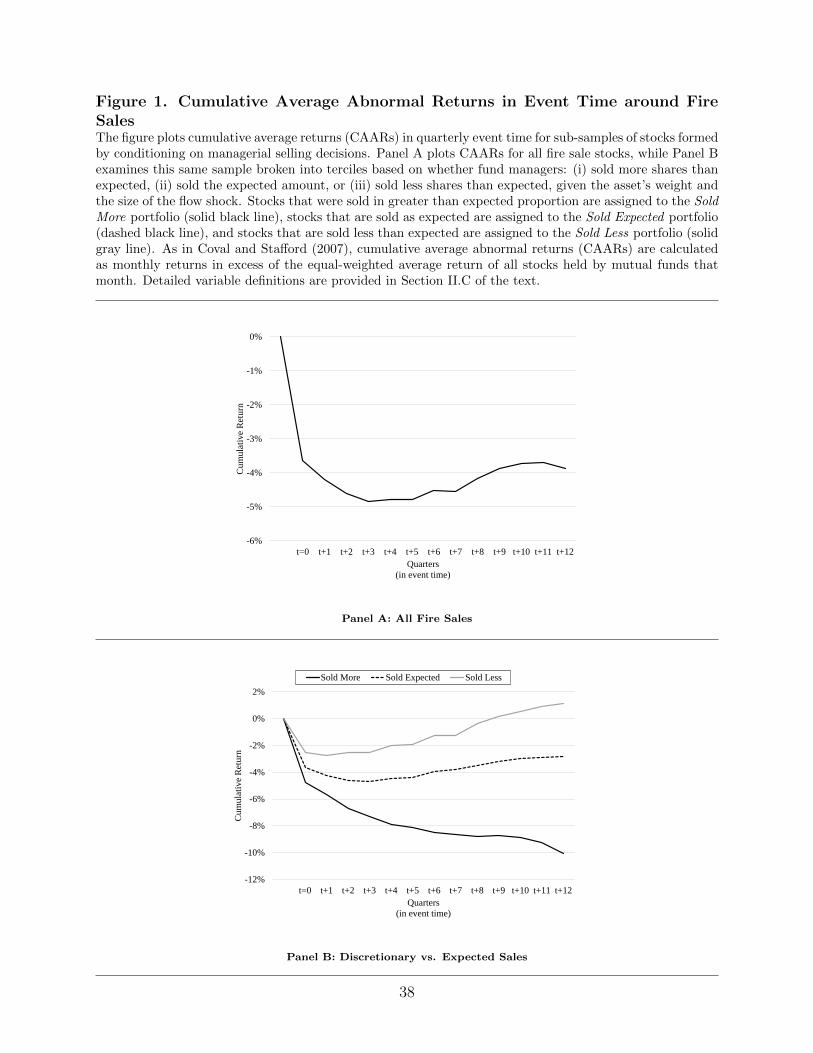
Figure 1. Cumulative Average Abnormal Returns in Event Time around FireSalesThe figure plots cumulative average returns (CAARs) in quarterly event time for sub-samples of stocks formedby conditioning on managerial selling decisions. Panel A plots CAARs for all fire sale stocks, while Panel Bexamines this same sample broken into terciles based on whether fund managers: (i) sold more shares thanexpected, (ii) sold the expected amount, or (iii) sold less shares than expected, given the asset’s weight andthe size of the flow shock. Stocks that were sold in greater than expected proportion are assigned to the SoldMore portfolio (solid black line), stocks that are sold as expected are assigned to the Sold Expected portfolio(dashed black line), and stocks that are sold less than expected are assigned to the Sold Less portfolio (solidgray line). As in Coval and Stafford (2007), cumulative average abnormal returns (CAARs) are calculatedas monthly returns in excess of the equal-weighted average return of all stocks held by mutual funds thatmonth. Detailed variable definitions are provided in Section II.C of the text.

-6%

-5%

-4%

-3%

-2%

-1%

0%

t=0 t+1 t+2 t+3 t+4 t+5 t+6 t+7 t+8 t+9 t+10 t+11 t+12

Cum

ula

tiv

e R

eturn

Quarters

(in event time)

Panel A: All Fire Sales

-12%

-10%

-8%

-6%

-4%

-2%

0%

2%

t=0 t+1 t+2 t+3 t+4 t+5 t+6 t+7 t+8 t+9 t+10 t+11 t+12

Cum

ula

tiv

e R

etu

rn

Quarters

(in event time)

Sold More Sold Expected Sold Less

Panel B: Discretionary vs. Expected Sales

38

Figure 2. Negative Information in Event Time around Fire SalesThe figure plots two proxy variables for negative information: (i) Short Interest (as apercent of shares outstanding) and (ii) future earnings surprises (EarnSurprise) calculatedusing a seasonally adjusted random walk model. Both variables are plotted in event timefor fire sale stocks (i.e., those in the bottom decile of Pressure) over the period 1990through 2015; the vertical gray bar at t = 0 indicates the fire sale quarter. Detailed variabledefinitions are provided in Section II.C of the text.

-0.2%

-0.2%

-0.1%

-0.1%

0.0%

0.1%

0.1%

0.2%

0.2%

4.1%

4.2%

4.3%

4.4%

4.5%

4.6%

4.7%

t-8 t-7 t-6 t-5 t-4 t-3 t-2 t-1 t=0 t+1 t+2 t+3 t+4 t+5 t+6 t+7 t+8

Sta

nd

ard

ized E

arn

ings S

urp

riseS

hort

In

tere

st

(As

a P

erc

en

t of

Sh

are

s O

uts

tan

din

g)

Quarter

(In Event Time)

Short Interest Earnings Surprise

39

Table ISummary Statistics

The sample includes all NYSE and NASDAQ common stocks (i.e., share codes 10 and 11)over the period January 1990 to December 2015. The mean, median, 1st percentile, 99thpercentile, and standard deviation of the following variables are reported: Pressure is ameasure of price pressure as defined in equation (2) and based on Coval and Stafford (2007)and Kahn, Kogan, and Serafeim (2012). ExpectedTradingi,t is the portion of Pressurethat equals fund flows prorated to the stock-level using each stock’s weight in the portfolio,and DiscretionaryTrading is the portion of Pressure this is not from ExpectedTrading.EarnSurprise is standardized unexpected earnings in the period after the fire sale calculatedusing a seasonally adjusted random walk model, Short Interest % is short interest as apercentage of shares outstanding, LN(Short Interest %) is the natural log of short interest asa percentage of shares outstanding, LN(Bid-Ask %) is the natural log of the bid-ask spreadas a fraction of the closing mid-point, and LN(Market Cap.) is the natural log of marketcapitalization in millions of U.S. dollars.

(1) (2) (3) (4) (5)Variable Mean Median 1st % 99th % St. Dev.Pressure 0.0005 0.0000 -0.0176 0.0222 0.0068Expected Trading 0.0009 0.0000 -0.0082 0.0200 0.0051Discrectionary Trading -0.0004 0.0000 -0.0237 0.0198 0.0074EarnSurprise 0.0000 0.0015 -0.1469 0.1307 0.0292Short Interest % 3.26% 1.43% 0.00% 23.67% 4.97%LN(Short Interest %) -4.7019 -4.2333 -11.0303 -1.4391 2.1039LN(Bid-Ask %) -5.0337 -4.6396 -8.8069 -2.1785 1.7114LN(Market Cap.) 19.6611 19.4849 16.3406 24.4744 1.8104

40

Table IITrading Decisions of Fire Sale Fund Managers

This table examines the trading decisions of funds during a fire sale quarter. Panel A displaysthe percent of positions within each distressed fund that were (1) decreased, (2) increased,or (3) held constant in the fire sale quarter. Panel B examines a linear probability model ofthe form:

1[Sell]i,t = β1StockCharacteristics+ FEi + FEt + εi,t, (10)

where 1[Sell]i,t is an indicator variable that takes the value one if asset i was sold by a distressedfund in quarter t, and zero otherwise, and StockCharacteristics is one of two proxy variablesfor information about the fundamental value of the firm, either: (i) LN(ShortInterest)i,t−1or (ii) future earnings surprises (EarnSurprisei,t+1). Distressed funds are funds in the top10% of outflows each quarter. In addition, we include two measures of firm liquidity: (i) thebid-ask spread and (ii) market capitalization. Firm fixed effects are included in all modelsand we include either date (year-quarter) or date × industry fixed effects, as indicated atthe bottom of the table. t-statistics calculated using standard errors clustered by firm anddate are shown below the estimates in italics. *, **, *** indicate statistical significance atthe 10%, 5%, and 1% levels, respectively.

Panel A: Trading Behavior of Fire Sale Funds

Decreased Increased Held Constant(1) (2) (3)

Percent of Positions 43.2% 19.6% 37.2%

Panel B: Linear Probability Model

Explanatory Dependent Variable: Sell IndicatorVariable (1) (2) (3) (4)

LN(Short Interest %) 0.0223*** 0.0217***(9.95) (9.85)

SUE -0.2314*** -0.2041***(-7.27) (-6.58)

LN(Bid-Ask %) -0.0159*** -0.0169*** -0.0076*** -0.0103***(-5.96) (-6.58) (-2.87) (-4.22)

LN(Market Cap.) 0.0996*** 0.1070*** 0.0942*** 0.0995***(20.11) (21.64) (16.39) (17.77)

Firm FE Yes Yes Yes YesDate FE Yes No Yes NoIndustry × Date FE No Yes No YesObservations 205,150 204,649 162,715 161,929R-squared 55.0% 57.2% 47.0% 50.7%

41

Table IIIDiscretionary and Expected Trading Decisions of Fire Sale Fund Managers

This table examines selling decisions by distressed funds according to an OLS panel modelof the form:

∆Holdingsi,t = β1StockCharacteristics+ Controls+ FEi + FEt + εi,t,

where ∆Holdingsi,t is either DiscretionaryTrading in models (1) and (2) orExpectedTradingi,t in models (3) and (4). ExpectedTradingi,t is the portion of Pressurethat equals fund flows prorated to the stock-level using each stock’s weight in the portfolio,and DiscretionaryTrading is the portion of Pressure this is not from ExpectedTrading.StockCharacteristics is one of two proxy variables for information about the fundamen-tal value of the firm, either: (i) LN(ShortInterest)i,t−1 or (ii) future earnings surprises(EarnSurprisei,t+1). In addition, we include two measures of firm liquidity: (i) the bid-askspread and (ii) market capitalization. Firm fixed effects and industry × date (year-quarter)fixed effects are included in all models. t-statistics calculated using standard errors clusteredby firm and date are shown below the estimates in italics. *, **, *** indicate statisticalsignificance at the 10%, 5%, and 1% levels, respectively.

Dependent Variable:Explanatory Discretionary Trading Expected TradingVariable (1) (2) (3) (4)

LN(Short Interest %)i,t−1 -0.0417** 0.0035(-2.16) (0.13)

SUEi,t+1 1.1935* 0.2532(1.70) (0.54)

LN(Bid-Ask %)i,t−1 0.0479 0.0358 -0.0576 -0.1025***(1.63) (1.13) (-1.48) (-2.89)

LN(Market Cap.)i,t−1 -0.2151*** -0.2600*** 0.1027 0.0571(-3.49) (-4.16) (1.56) (0.82)

Firm FE Yes Yes Yes YesIndustry × Date FE Yes Yes Yes YesObservations 204,649 161,929 204,649 161,929R-squared 10.4% 10.3% 22.8% 22.8%

42

Table IVAbnormal Returns in Event Time around Fire Sales

The table displays monthly abnormal returns and cumulative abnormal returns (CAAR)in event time around fire sales, where the event quarter (t=0) is the quarter in which astock had intensive selling pressure. ExpectedTradingi,t is the portion of Pressure thatequals fund flows prorated to the stock-level using each stock’s weight in the portfolio andDiscretionaryTrading is the portion of Pressure this is not from ExpectedTrading. Eachquarter, all fire sale stocks are sorted into terciles based on DiscretionaryTrading. Stocksin the lowest tercile had more selling pressure than expected (Sold More), stocks in themiddle tercile had selling pressure approximately equal to the expected selling pressure (SoldExpected), and stocks in the highest tercile had less selling pressure than expected (SoldLess). We form portfolio based on these terciles and examine returns in event time. As inCoval and Stafford (2007), abnormal returns are calculated as monthly returns in excess ofthe equal-weighted average return of all stocks held by mutual funds that month. The tablereports the mean abnormal return in columns (1) through (3) and the cumulative averageabnormal return (CAAR) in columns (4) through (6).

Monthly Average Abnormal Return Cumulative Average Abnormal ReturnEvent Sold Less Sold Expected Sold More Sold Less Sold Expected Sold MoreTime (1) (2) (3) (4) (5) (6)

t=0 -2.5% -3.6% -4.8% -2.54% -3.62% -4.75%t+1 -0.2% -0.6% -0.9% -2.75% -4.21% -5.64%t+2 0.2% -0.4% -1.1% -2.55% -4.59% -6.73%t+3 0.0% -0.1% -0.6% -2.52% -4.69% -7.32%t+4 0.6% 0.2% -0.6% -1.97% -4.49% -7.91%t+5 0.0% 0.1% -0.2% -1.92% -4.38% -8.12%t+6 0.7% 0.4% -0.3% -1.26% -3.94% -8.47%t+7 0.0% 0.1% -0.2% -1.24% -3.81% -8.68%t+8 0.9% 0.3% -0.1% -0.36% -3.49% -8.76%t+9 0.5% 0.3% 0.0% 0.16% -3.19% -8.73%t+10 0.4% 0.2% -0.2% 0.51% -2.95% -8.90%t+11 0.4% 0.1% -0.3% 0.89% -2.88% -9.22%t+12 0.2% 0.0% -0.8% 1.11% -2.86% -10.04%

43

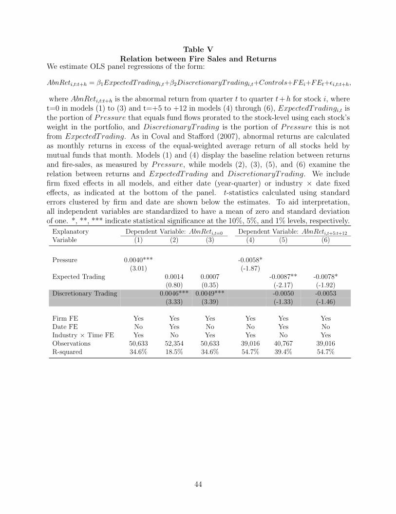
Table VRelation between Fire Sales and Returns

We estimate OLS panel regressions of the form:

AbnReti,t:t+h = β1ExpectedTradingi,t+β2DiscretionaryTradingi,t+Controls+FEi+FEt+εi,t:t+h,

where AbnReti,t:t+h is the abnormal return from quarter t to quarter t+h for stock i, wheret=0 in models (1) to (3) and t=+5 to +12 in models (4) through (6), ExpectedTradingi,t isthe portion of Pressure that equals fund flows prorated to the stock-level using each stock’sweight in the portfolio, and DiscretionaryTrading is the portion of Pressure this is notfrom ExpectedTrading. As in Coval and Stafford (2007), abnormal returns are calculatedas monthly returns in excess of the equal-weighted average return of all stocks held bymutual funds that month. Models (1) and (4) display the baseline relation between returnsand fire-sales, as measured by Pressure, while models (2), (3), (5), and (6) examine therelation between returns and ExpectedTrading and DiscretionaryTrading. We includefirm fixed effects in all models, and either date (year-quarter) or industry × date fixedeffects, as indicated at the bottom of the panel. t-statistics calculated using standarderrors clustered by firm and date are shown below the estimates. To aid interpretation,all independent variables are standardized to have a mean of zero and standard deviationof one. *, **, *** indicate statistical significance at the 10%, 5%, and 1% levels, respectively.

Explanatory Dependent Variable: AbnReti,t=0 Dependent Variable: AbnReti,t+5:t+12

Variable (1) (2) (3) (4) (5) (6)

Pressure 0.0040*** -0.0058*(3.01) (-1.87)

Expected Trading 0.0014 0.0007 -0.0087** -0.0078*(0.80) (0.35) (-2.17) (-1.92)

Discretionary Trading 0.0046*** 0.0049*** -0.0050 -0.0053(3.33) (3.39) (-1.33) (-1.46)

Firm FE Yes Yes Yes Yes Yes YesDate FE No Yes No No Yes NoIndustry × Time FE Yes No Yes Yes No YesObservations 50,633 52,354 50,633 39,016 40,767 39,016R-squared 34.6% 18.5% 34.6% 54.7% 39.4% 54.7%

44

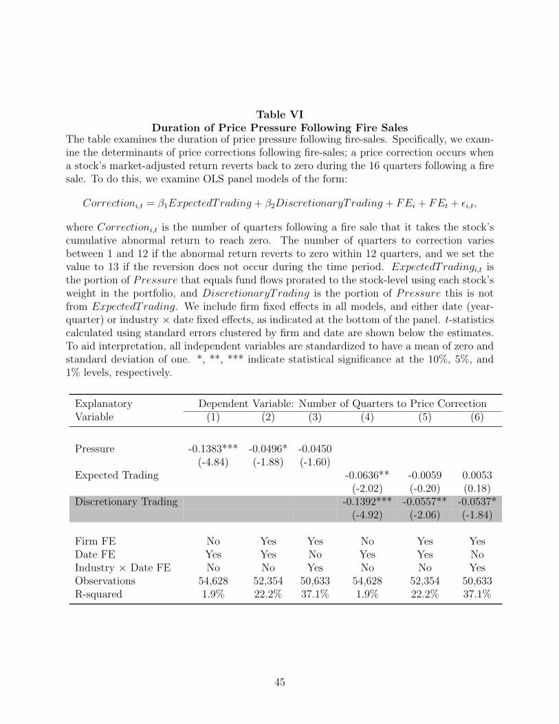
Table VIDuration of Price Pressure Following Fire Sales

The table examines the duration of price pressure following fire-sales. Specifically, we exam-ine the determinants of price corrections following fire-sales; a price correction occurs whena stock’s market-adjusted return reverts back to zero during the 16 quarters following a firesale. To do this, we examine OLS panel models of the form:

Correctioni,t = β1ExpectedTrading + β2DiscretionaryTrading + FEi + FEt + εi,t,

where Correctioni,t is the number of quarters following a fire sale that it takes the stock’scumulative abnormal return to reach zero. The number of quarters to correction variesbetween 1 and 12 if the abnormal return reverts to zero within 12 quarters, and we set thevalue to 13 if the reversion does not occur during the time period. ExpectedTradingi,t isthe portion of Pressure that equals fund flows prorated to the stock-level using each stock’sweight in the portfolio, and DiscretionaryTrading is the portion of Pressure this is notfrom ExpectedTrading. We include firm fixed effects in all models, and either date (year-quarter) or industry × date fixed effects, as indicated at the bottom of the panel. t-statisticscalculated using standard errors clustered by firm and date are shown below the estimates.To aid interpretation, all independent variables are standardized to have a mean of zero andstandard deviation of one. *, **, *** indicate statistical significance at the 10%, 5%, and1% levels, respectively.

Explanatory Dependent Variable: Number of Quarters to Price CorrectionVariable (1) (2) (3) (4) (5) (6)

Pressure -0.1383*** -0.0496* -0.0450(-4.84) (-1.88) (-1.60)

Expected Trading -0.0636** -0.0059 0.0053(-2.02) (-0.20) (0.18)

Discretionary Trading -0.1392*** -0.0557** -0.0537*(-4.92) (-2.06) (-1.84)

Firm FE No Yes Yes No Yes YesDate FE Yes Yes No Yes Yes NoIndustry × Date FE No No Yes No No YesObservations 54,628 52,354 50,633 54,628 52,354 50,633R-squared 1.9% 22.2% 37.1% 1.9% 22.2% 37.1%

45

Table VIIDiscretionary Trading by Non-Fire Sale Funds

This table examines trading decisions by non-distressed funds according to an OLS panelmodel of the form:

DiscretionaryTradingi,t = β1 + Controls+ FEi + FEt + εi,t,

where DiscretionaryTrading is discretionary trading by funds that are not experiencingfire sales. ExpectedTradingF ireSales is expected trading by funds experiencing a firesale last period and DiscretionaryTradingF ireSales is discretionary trading by fundsexperiencing a fire sale last period. Controls include the natural log of short interest(LN(ShortInterest)i,t−1), future earnings surprises (EarnSurprisei,t+1), the bid-ask spread(LN(Bid−Ask%i,t−1)), and the natural log of market capitalization (LN(MarketCapi,t−1)).Firm fixed effects are included in all models and industry × date (year-quarter) fixed effectsare included in even numbered models. t-statistics calculated using standard errors clusteredby firm and date are shown below the estimates in italics. *, **, *** indicate statistical sig-nificance at the 10%, 5%, and 1% levels, respectively.

Dependent Variable:Explanatory Discretionary trading by non-fire sale fundsVariable (1) (2) (3) (4)

Expected Trading Fire Salei,t−1 0.0007*** 0.0007*** 0.0007** 0.0006***(7.35) (10.50) (2.39) (6.40)

Discretionary Trading Fire Salei,t−1 0.0008*** 0.0008*** 0.0008*** 0.0009***(11.73) (11.22) (13.54) (15.65)

LN(Short Interest %)i,t−1 -0.0007 -0.0008**(-0.64) (-2.58)

SUEi,t+1 0.0154 0.0002(0.53) (0.03)

LN(Bid-Ask %)i,t−1 0.0003 -0.0003(0.45) (-1.34)

LN(Market Cap.)i,t−1 0.0007 0.0016***(0.33) (3.08)

Firm FE Yes Yes Yes YesIndustry × Date FE No Yes No YesObservations 456,600 455,918 125,914 125,479R-squared 4.8% 18.1% 4.1% 28.7%

46

Table VIIITest of Theoretical Relation between Adverse Selection and Price Pressure

The table examines the relation between trading, price pressure, and variables that theoreticallyexacerbate adverse selection using panel regressions of the form:

AbnReti,t = β1ExpectedTradingi,t + β2DiscretionaryTradingi,t + β3Si,t + ΓXi,t + FEi + εi,t,

where AbnReti,t is the abnormal return in quarter t=0, where t=0 is the quarter of the fire sale for

stock i, ExpectedTradingi,t is the portion of Pressure that equals fund flows prorated to the stock-

level using each stock’s weight in the portfolio, DiscretionaryTrading is the portion of Pressure

this is not from ExpectedTrading, Si,t is either (i) an indicator variable that takes the value

one if a stock is held by funds that have more than 2% of net assets in cash and zero otherwise

(Cash) or (ii) an indicator variables that takes the value one if the VIX is above 40 and zero

otherwise (Stress), and Xi,t is a vector of interaction terms that contain ExpectedTrading × Si,tand DiscretionaryTrading×Si,t. As in Coval and Stafford (2007), abnormal returns are calculated

as monthly returns in excess of the equal-weighted average return of all stocks held by mutual funds

that month. Models (1), (2), and (5) display the baseline relation between future returns and fire-

sales, as measured by Pressure, while models (3), (4), and (6) examine the relation between future

returns and ExpectedTrading and DiscretionaryTrading. We include firm fixed effects in all

models, and date (year-quarter) or industry × date fixed effects, as indicated at the bottom of the

panel. t-statistics calculated using standard errors clustered by firm and date are shown below the

estimates. To aid interpretation, all independent variables are standardized to have a mean of zero

and standard deviation of one. *, **, *** indicate statistical significance at the 10%, 5%, and 1%

levels, respectively.

Explanatory Dependent Variable: Abnormal Announcement Quarter ReturnVariables (1) (2) (3) (4) (5) (6)Pressure 0.1532 0.1538 0.4624**

(0.71) (0.65) (2.14)Expected Trading 0.3456 0.4178 -0.0799

(0.69) (0.66) (-0.21)Discretionary Trading 0.0974 0.0887 0.5778**

(0.39) (0.34) (2.59)Cash Indicator 0.0071 0.0073 0.0071 0.0073

(1.51) (1.56) (1.50) (1.54)Pressure × Cash 0.4693 0.4866

(1.57) (1.57)Expected × Cash -0.0743 -0.3261

(-0.14) (-0.51)Discretionary × Cash 0.5937* 0.6571**

(1.81) (2.00)Stress Indicator 0.0121* 0.0121*

(1.89) (1.89)Pressure × Stress 1.1546**

(2.21)Expected × Stress 1.7662**

(2.37)Discretionary × Stress 1.0211*

(1.92)Firm FE Yes Yes Yes Yes Yes YesDate FE Yes No Yes No No NoIndustry × Date FE No Yes No Yes No NoObservations 52,354 50,633 52,354 50,633 52,354 52,354R-squared 18.5% 34.6% 18.5% 34.6% 16.5% 16.5%

47

Table IXFive-Factor Alphas from Portfolios formed on Discretionary Trades around

Fire SalesThe table examines five-factor (Fama and French (2015)) alphas from portfolios formed byconditioning on the discretionary selling decisions of stocks that are experiencing fire sales.We calculate ExpectedTrading as the portion of Pressure that equals fund flows proratedto the stock-level using each stock’s weight in the portfolio, and DiscretionaryTrading asthe portion of Pressure this is not from ExpectedTrading. We then rank all fire sale stocksinto terciles based on DiscretionaryTrading. Column (2) shows the alpha (intercept) andfactor loads associated with a portfolio that is formed by buying fire sale stocks in tercile 1 ofDiscretionaryTrading, which consists of stocks with greater than expected selling pressure.Column (4) shows the alpha (intercept) and factor loads associated with a portfolio that isformed by buying fire sale stocks in tercile 3 of DiscretionaryTrading, which consists ofstocks with lower than expected selling pressure. Finally, column (6) shows the alpha toa long-short portfolio that buys stocks with lower than expected selling pressure and shortsells stocks with higher than expected selling pressure. t-statistics, calculated using standarderrors clustered by firm, are shown next to the coefficient estimates in italics. In Panel A,we examine abnormal returns to a portfolio that begins 5 quarters after the event date andholds stocks until quarter t+8. In Panel B, we examine annualized abnormal returns to aportfolio that begins 5 quarters after the event date and holds stocks until quarter t+12.

Panel A: Holding period = quarter t+5 through quarter t+8

(1) (2) (3) (4) (5) (6)Explanatory Sold More Sold Less Long-ShortVariable Estimate t-stat Estimate t-stat Estimate t-stat

Intercept (α) -1.1256** (-2.10) 0.8190* (1.66) 1.9446*** (2.90)Mkt 0.1475 (1.17) 0.2452** (2.13)SMB -0.7590*** (-3.88) -0.6131*** (-3.42)HML -0.6131*** (-2.77) -0.4245** (-2.02)RMW -0.4615** (-2.39) -0.4433*** (-2.59)CMA 1.7338*** (5.77) 1.3646*** (4.79)

Panel B: Holding period = quarter t+5 through quarter t+12Explanatory Sold More Sold Less Long-ShortVariable Estimate t-stat Estimate t-stat Estimate t-stat

Intercept (α) -0.0718 (-0.16) 2.0915*** (5.08) 2.1633*** (3.97)Mkt -0.1548* (-1.73) 0.0030 (0.04)SMB 0.4608*** (3.32) 0.1744 (1.40)HML 0.2873 (1.57) -0.1226 (-0.78)RMW 0.1087 (0.56) 0.4881*** (2.90)CMA -0.6001** (-2.27) -0.1483 (-0.62)

48

V. Appendix

This appendix provides additional empirical evidence to supplement the analyses provided

in the main text. Below, we briefly discuss each of the included figures and tables.

• In Figure A1 we plot the returns to fire sale stocks split on two proxies for fundamental

information: Short Interest and EarnSurprise. The results show that fire sale stocks

with high short interest earn abnormally low returns that do not reverse, while fire

sales stocks with low short interest experience small price drops that quickly correct.

Similarly, fire sale stocks with negative future earnings surprises earn abnormally low

future returns that do not reverse, while fire sales stocks with positive future earnings

surprises experience small price drops that quickly correct.

• In Table A1 we display a correlation matrix of the variables used in the main text.

• In Table A2 we examine whether mutual fund managers use their selling skill during

all periods (not just those with fire sales). To do this, we modify equations (3) and

(4) in the main text so that they do not condition on the magnitude of flow shocks.

Specifically, we calculate a measure of expected trading in each period (regardless of

flow magnitude) according to the equation:

ExpectedTradingNoFirei,t =

∑j

(Holdingsj,i,t−1 × flowj,t)

SharesOutstandingi,t−1. (11)

We then calculate a measure of discretionary trading by fund managers regardless of

flow magnitude according to the equation:

DiscretionaryTradingNoFirei,t = ActualTradesi,t − ExpectedTradingNoFirei,t,

(12)

where ActualTradesi,t is the actual change in holdings by mutual funds between period

t−1 and t for stock i. The results in Table A2 shows that fund managers are more likely

49

to have discretionary sales in stocks with high short interest in all periods regardless of

flow shocks (model (1)). Moreover, consistent with the placebo test in the main text,

we find that expected trading is never related to stock characteristics (model (2)).

• In Table A3 we examine a linear probability model of the determinants of whether

or not cumulative average abnormal returns revert to zero during the twelve quarters

following fire-sales.

• In Section V.A, we provide a detailed discussion of the requirements for a valid proxy

variable.

50

Figure A1. Cumulative Average Abnormal Returns in Event Time around Fire-Sales for High and Low Quality StocksThe figure plots cumulative average returns (CAARs) in quarterly event time for sub-samples of stocksformed using two different proxy variables for negative information: (i) Short Interest (as a percent of sharesoutstanding) and (ii) future earnings surprises (EarnSurprise) calculated using a seasonally adjusted randomwalk model. Each quarter, stocks in the bottom decile of Pressure are grouped into two portfolios, basedon a proxy variable for negative information. In Panel A, we use short interest in the quarter prior to theevent quarter as the proxy variable: stocks above the sample median value of short interest are assigned tothe High Short Interest portfolio (dashed line), and stocks at or below the median value are assigned to theLow Short Interest portfolio (solid line). In Panel B, we use earnings surprise in the quarter after the eventquarter as the proxy variable: stocks with a negative value of EarnSurprise are assigned to the NegativeEarnings Surprise portfolio (dashed line), and stocks with a positive value of EarnSurprise are assigned tothe Positive Earnings Surprise portfolio (solid line). As in Coval and Stafford (2007), cumulative averageabnormal returns (CAARs) are calculated as monthly returns in excess of the equal-weighted average returnof all stocks held by mutual funds that month. Detailed variable definitions are in Section II.C of the text.

0

0.1

0.2

0.3

0.4

0.5

0.6

0.7

0.8

0.9

1

-0.15

-0.1

-0.05

0

0.05

0.1

0.15

0.2

t-3 t-2 t-1 t=0 t+1 t+2 t+3 t+4 t+5 t+6 t+7 t+8

Cum

ulat

ive

Ret

urn

Quarters(in event time)

Low Short Interest Stocks High Short Interest Stocks

Panel A: Short Interest

0

0.1

0.2

0.3

0.4

0.5

0.6

0.7

0.8

0.9

1

-0.25

-0.2

-0.15

-0.1

-0.05

0

0.05

0.1

0.15

t-3 t-2 t-1 t=0 t+1 t+2 t+3 t+4 t+5 t+6 t+7 t+8

Cum

ulat

ive

Ret

urn

Quarters(in event time)

Pos. Earn Surprise Neg. Earn Surprise

Panel B: Future Earnings Surprises

51

Table A1Correlation Matrix

The table displays a correlation matrix of the variables used in the main paper. Pearson correlations are shown below the diagonaland Spearman correlations are shown above the diagonal. The price pressure measure, Pressure, is defined in equation (2) andbased on Coval and Stafford (2007) and Kahn, Kogan, and Serafeim (2012). ExpectedTradingi,t is the portion of Pressurethat equals fund flows prorated to the stock-level using each stock’s weight in the portfolio, and DiscretionaryTrading is theportion of Pressure this is not from ExpectedTrading. EarnSurprise is standardized earnings surprises in the period after thefire sale calculated using a seasonally adjusted random walk model, LN(Short Interest %) is the natural log of short interest as apercentage of shares outstanding, LN(Bid-Ask %) is the natural log of the bid-ask spread as a fraction of the closing mid-point,and LN(Market Cap.) is the natural log of market capitalization in millions of U.S. dollars.

Pressu

re

Exp

ectedT

radin

g

Discrection

aryT

radin

g

Earn

Surp

rise

LN

(Short

Interest

%

LN

(Bid

-Ask

%)

LN

(Market

Cap

.)

Pressure 1.00 0.57 0.58 0.01 0.02 -0.03 -0.02Expected Trading 0.40 1.00 -0.15 0.02 0.04 -0.05 0.01Discrectionary Trading 0.80 -0.24 1.00 -0.01 -0.04 0.02 0.00EarnSurprise 0.00 0.01 0.00 1.00 -0.03 0.00 0.01LN(Short Interest %) 0.00 0.03 -0.02 -0.01 1.00 -0.34 0.01LN(Bid-Ask %) 0.01 -0.01 0.01 -0.02 -0.40 1.00 -0.42LN(Market Cap.) -0.03 -0.05 0.00 0.01 0.11 -0.40 1.00

52

Table A2Discretionary and Expected Trading Decisions of Fund Managers without

Conditioning on the occurrence of Fire SalesThis table examines selling decisions by all mutual funds according to an OLS panel modelof the form:

∆Holdingsi,t = β1StockCharacteristics+ Controls+ FEi + FEt + εi,t,

where ∆Holdingsi,t is DiscretionaryTrading in model (1) and ExpectedTradingi,t in model(2). The specifications are similar to Table III of the main text, which shows the determinantsof trading decisions by fund managers experiencing large flow shocks, except they look atall trades, not just trades that occurred following large flow shocks. ExpectedTradingi,t isthe portion of Pressure that equals fund flows prorated to the stock-level using each stock’sweight in the portfolio, andDiscretionaryTrading is the portion of Pressure this is not fromExpectedTrading. StockCharacteristics is one of two proxy variables for information aboutthe fundamental value of the firm, either: (i) LN(ShortInterest)i,t−1 or (ii) future earningssurprises (EarnSurprisei,t+1). In addition, we include two measures of firm liquidity: (i)the bid-ask spread and (ii) market capitalization. Firm fixed effects and industry × date(year-quarter) fixed effects are included in all models. Standard errors clustered by firm anddate are shown below the estimates in italics. *, **, *** indicate statistical significance atthe 10%, 5%, and 1% levels, respectively.

Dependent Variable:Explanatory Discretionary Trading Expected TradingVariables (1) (2)

LN(Short Interest %)i,t−1 -0.0009*** 0.0000(-2.93) (1.35)

SUEi,t+1 0.0020 0.0001(0.30) (1.04)

LN(Bid-Ask %)i,t−1 -0.0003 0.0000(-1.41) (1.01)

LN(Market Cap.)i,t−1 0.0018*** 0.0000(3.25) (0.61)

Firm FE Yes YesIndustry × Date FE Yes YesObservations 125,524 125,524R-squared 27.0% 36.1%

53

Table A3Linear Probability Model of Price Corrections Following Fire Sales

The table examines whether cumulative average abnormal returns revert to zero duringthe twelve quarters following fire-sales. Specifically, we examine the determinants of pricecorrections following fire sales. To do this, we examine linear probability panel models ofthe form:

1Correctioni,t= β1ExpectedTrading + β2DiscretionaryTrading + FEi + FEt + εi,t,

where 1Correctioni,tis an indicator variable that takes the value one if a stock’s cumulative

abnormal return reverts to zero within twelve quarters of a fire sale, and zero otherwise.ExpectedTradingi,t is the portion of Pressure that equals fund flows prorated to the stock-level using each stock’s weight in the portfolio, and DiscretionaryTrading is the portionof Pressure this is not from ExpectedTrading. We include fixed effects in all models, asindicated at the bottom of the panel. t-statistics calculated using standard errors clusteredby firm and year-quarter are shown below the estimates. *, **, *** indicate statisticalsignificance at the 10%, 5%, and 1% levels, respectively.

Explanatory Dependent Variable: Indicator Variable for Price CorrectionVariable (1) (2) (3) (4) (5) (6)

Pressure 0.0099*** 0.0034* 0.0029(4.85) (1.76) (1.42)

Expected Trading 0.0034 -0.0006 -0.0010(1.62) (-0.29) (-0.46)

Discretionary Trading 0.0104*** 0.0041** 0.0037*(5.03) (2.13) (1.76)

Firm FE No Yes Yes No Yes YesDate FE Yes Yes No Yes Yes NoIndustry × Date FE No No Yes No No YesObservations 54,628 52,354 50,633 54,628 52,354 50,633R-squared 2.8% 24.7% 37.6% 2.8% 24.7% 37.6%

54

A. Formal Requirements for a Valid Proxy Variable

Wooldridge (2010) discusses the requirements for a valid proxy variable. Formally, there are

two requirements for a variable, z, to be valid proxy variable for a latent variable q:

1. E[y | x, q, z] = E[y | x, q]

2. L[q | 1, x1, . . . , xK , z] = L[q | 1, z],

where E[·] is the expectations operator and L[·] is a linear projection operator. The first

condition says that the proxy variable z is not related to y after accounting for q. In

our case, this condition seems uncontroversial and implies that short interest or earnings

surprises would not be related to fire sales if we could control for the actual quantity of

negative information about a stock. The second condition is more complicated, and is

similar to an exclusion restriction in a standard instrumental variables model. It requires the

correlation between the latent variable q and each covariate x to be zero after we include the

proxy variable z. Of course, since q is unobservable, this restriction is inherently untestable.

However, Wooldridge (2010) notes that even if z is an imperfect proxy such that the second

condition does not hold, it is likely that the Ordinary Least Squares (“OLS”) estimator

will be better than if no proxy variable is included. Accordingly, we proceed by defining

ShortInteresti,t−1 and EarnSurprisei,t+1 as our proxy variables for unobservable negative

information about stock i in quarter t.

55