Title Page

TITLE:

TECHNOLOGICAL DEVELOPMENTS ALLOWING FOR THE WIDESPREAD

CLINICAL ADOPTION OF PROTON RADIOTHERAPY.

Researcher/Investigator: Andries Nicolaas (Niek) Schreuder

INSTITUTION: UCL - University College London

RESEARCH DEGREE: PHD - MEDICAL PHYSICS & BIOENGINEERING

Date: March 2020

Declaration of Confidentiality:

This thesis does not contain any confidential or private patient data. All included patient

information is anonymized.

Declaration of Authenticity:

I, Andries Nicolaas (Niek) Schreuder confirm that the work presented in this thesis is my own.

Where information has been derived from other sources, I confirm that this has been indicated in

the thesis.

ACKNOWLEDGEMENTS

I would like to express my appreciation and gratitude to:

Professor Gary Royle for his leadership and guidance and even more importantly his

enthusiasm in nudging me along to get the thesis finished and submitted.

Richard Amos who introduced me to Professor Royle and UCL.

My wife Therese and the rest of the family for their support and motivation to continue to

pursue my dream of obtaining a PhD in medical physics. I want to specially thank Lia for the

endless hours wordsmithing the text and correcting the tenses and typos.

My colleagues at Provision Healthcare for numerous discussions and support during the

experimental and data analysis phases of the work.

Daniel Bridges for helping me to get the two most important peer reviewed papers

published and Jacob Shamblin for co-authoring the third paper.

All the numerous scientists that I worked with at iThemba Labs, Indiana University,

ProCure and Provision as well as the leadership of these organizations for providing the means

for me to innovate and to develop the skills and technologies documented in this work.

Most significantly to my Heavenly Father that blessed me with the skills and opportunities

to do this. In 2 Corinthians 12 the apostle Paul talks about his “thorn in the flesh” that kept him

from exalting in himself. For many years not having a PhD in Medical physics served the same

purpose for me. However, I will ensure that I will never exalt in my own skills but only in my

weaknesses since “God’s grace is sufficient for me and His power is perfected in my

weaknesses”.

This thesis is dedicated to my parents – the late Amos Schreuder and Dina Schreuder

who gave me the foundation to pursue college and a professional career.

ABSTRACT

External beam radiation therapy using accelerated protons has undergone significant

development since the first patients were treated with accelerated protons in 1954. Widespread

adoption of proton therapy is now taking place and is fully justified based on early clinical and

technical research and development. Two of the main advantages of proton radiotherapy are

improved healthy tissue sparing and increased dose conformation. The latter has been improved

dramatically through the clinical realization of Pencil Beam Scanning (PBS). Other significant

advancements in the past 30 years have also helped to establish proton radiotherapy as a major

clinical modality in the cancer-fighting arsenal. Proton radiotherapy technologies are constantly

evolving, and several major breakthroughs have been accomplished which could allow for a major

revolution in proton therapy if clinically implemented.

In this thesis, I will present research and innovative developments that I personally initiated or

participated in that brought proton radiotherapy to its current state as well as my ongoing

involvement in leading research and technological developments which will aid in the mass

adoption of proton radiotherapy. These include beam dosimetry, patient positioning technologies,

and creative methods that verify the Monte Carlo dose calculations which are now used in proton

treatment planning. I will also discuss major technological advances concerning beam delivery

that should be implemented clinically and new paradigms towards patient positioning. Many of

these developments and technologies can benefit the cancer patient population worldwide and

are now ready for mass clinical implementation. These developments will improve proton

radiotherapy efficiencies and further reduce the cost of proton therapy facilities.

This thesis therefore reflects my historical and ongoing efforts to meet market costs and time

demands so that the clinical benefit of proton radiotherapy can be realized by a more significant

fraction of cancer patients worldwide.

IMPACT STATEMENT

Proton radiation therapy has been used clinically since 1954 and major advancements in the past

10 years have helped establish protons as a major clinical modality in the cancer fighting arsenal.

It is hard to argue against the use of protons for treating most solid tumors when looking only at

the physical dose distributions obtained from proton beams. However, considering the traditional

means to deliver the calculated doses to the patient in a reliable and trustworthy manner, many

scholars in the field are starting to question the promise and validity of proton therapy. The main

reason for this is the high costs of a classical proton therapy facility. The three most important

cost drivers are: the physical size of the proton therapy equipment that requires large and

expensive buildings, the actual cost of the equipment, the time needed to construct and

commission a proton therapy facility. Many of the existing proton therapy facilities across the

globe are fighting dire financial circumstances and some facilities have gone through financial

restructuring and even bankruptcies and closures. The work presented in thesis is very timely in

this regard. It addresses the historical perspectives of proton therapy and developments that are

leading the field into a new era of proton therapy. The proton therapy industry is now ready for

new paradigms in proton beam delivery and patient positioning that will reduce the cost of proton

therapy dramatically while improving efficiencies and the quality of proton beam delivery.

The thesis provides essential background information on proton therapy developments that can

be used by existing and future scholars in proton medical physics. The thesis describes the major

technological advances that helped to bring proton therapy to a level ready for mass adoption and

new technologies that are now ready for implementation and encourages vendors to bring these

to market. The new paradigms in patient positioning, e.g. upright treatments, bring new research

challenges to academia that should be exploited. Such research can and should be translated to

the proton therapy industry in the pursuit of reducing the costs of proton therapy.

It will be possible to install future proton therapy equipment in existing radiation therapy facilities,

obviating the need to build new and expensive buildings. This will reduce the time between project

inception and first patient treatments which will have a huge financial impact on the industry and

allow for proton facilities to operate in a more comfortable financial climate. This will provide

financial resources to academia to conduct the research mentioned in the thesis. Most

importantly it will be possible to offer proton therapy to patients at a lower cost which should be

the ultimate goal.

After reading this thesis, the reader will be aware of the clinical benefits of proton therapy and the

need to make it available to many more patients at affordable rates. The reader will understand

that the proton therapy industry is now ready for a paradigm shift in how patients are treated.

TABLE OF CONTENTS

1. Chapter 1: Thesis Overview and Scientific and Technical Contributions to

the Field of Proton Therapy . . . . . . . . . . . . . . . . . . . . . . . . . . . . . . . . . . . . . . . . . . . 15

2. Chapter 2: Proton Therapy and the Historic Developments That Enabled Proton

Therapy to Become Major Clinical Tool in Radiation Therapy . . . . . . . . . . . . . . . . . . 25

2.1. Introduction

2.2. Proton Radiation Therapy

2.2. History of Proton Radiation Therapy

2.3. Proton Therapy Today and the Years Ahead

2.4. Summary

3. Chapter 3: Earlier Proton Therapy Systems and Important Fundamental

Developments. . . . . . . . . . . . . . . . . . . . . . . . . . . . . . . . . . . . . . . . . . . . . . . . . . . . . . . . 35

3.1. Introduction

3.2. Proton Therapy at IThemba Labs

3.3. Proton Therapy at IUHPTC

3.4. Developments at Procure Treatment Centers

3.5. Summary

4. Chapter 4: The Clinical Realization of Pencil Beam Scanning and the Enormous

Impact on the Usability of Protons in Clinical Practice . . . . . . . . . . . . . . . . . . . . . . . . 71

4.1. Overview

4.2. Introduction

4.3. Technology Developments – Pencil Beam Scanning

4.4. Advances and Efficiencies in PBS Treatment Planning

4.5. Clinical Aspects of PBS Treatment

4.6. Summary

4.7.

5. Chapter 5: What is Needed in the Next Ten Years to Allow for the Mass Adoption

of Proton Therapy . . . . . . . . . . . . . . . . . . . . . . . . . . . . . . . . . . . . . . . . . . . . . . . . . . . . 90

5.1. Overview

5.2. Proton Therapy Special Feature: Review Article: Proton Therapy Delivery:

What is Needed in the Next Ten Years?

5.3. Optical Guidance to Supplement 3D Volumetric Image Guidance

5.4. The Case for Upright Treatments

5.5. Efficiencies in Proton Therapy Clinical Operations

6. Chapter 6: Validating the RayStation Monte Carlo Dose Calculation Algorithms

Using Realistic Phantoms . . . . . . . . . . . . . . . . . . . . . . . . . . . . . . . . . . . . . . . . . . . . . . 117

6.1. Overview

6.2. Peer Reviewed Paper 1 – MC Validation for Static Targets

6.3. Peer Reviewed Paper 2 – MC Validation for Lung Targets

6.4. Acknowledgments

7. Chapter 7: Summary and Concluding Remarks on the Work Presented in This

Thesis. . . . . . . . . . . . . . . . . . . . . . . . . . . . . . . . . . . . . . . . . . . . . . . . . . . . . . . . . . . . 156

8. References . . . . . . . . . . . . . . . . . . . . . . . . . . . . . . . . . . . . . . . . . . . . . . . . . . . .. . . . . 158

LIST OF FIGURES

Figure 2.1. Depth dose curves for an 8 MV x-ray beam (Dash-dot-dot line) and a 200 MeV proton

beam (solid lines). The thinner solid lines show Bragg peaks for proximal energy layers stacked onto the deepest energy layer to constitute the Spread-Out Bragg Peak (Dashed line) required to cover the target area (shaded).

Figure 2.2. The evolution of cyclotrons. The acceleration diameter (Blue bars) in inches and energy in MeV (red line) is illustrated against the year the cyclotron was built.

Figure 2.3. A schematic illustration of the first utilization of protons. Panel A shows the use of the Bragg peak as proposed by Wilson while panel B shows how the first treatments were done using the shoot through technique. Panel C shows a shoot through plan on a patient treated for a Pituitary lesion using the shoot through technique.

Figure 2.4. Excerpts from Goitein’s 1983 paper illustrating the concepts of the Beam’s eye view and the DRR.

Figure 2.5. Excerpts from Petti’s 1992 paper showing dose distributions of a proton beam traversing a slab of bone equivalent material calculated with ray-tracing, pencil beam and Monte Carlo algorithms.

Figure 3.1. A schematic layout of the NAC fixed horizontal beamline that was initially designed for radio surgery purposes only.

Figure 3.2. The measured depth dose curves for different field diameters (cm) see ref [2.28].

Figure 3.3. The penumbra for the NAC radiosurgery beam as a function of depth.

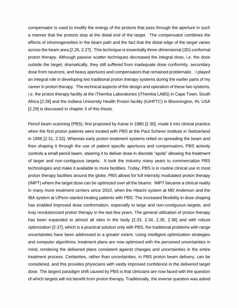
Figure 3.4. A schematic illustration of the occluding ring system

Figure 3.5. A schematic illustration of the MLIC range monitor that also served as a beam anti-scatter collimator. The panel on the right shows the Bragg Peak in Brass measured with the MLIC

Figure 3.6. A picture of the brass MLFC and anti-scatter small collimator

Figure 3.7. A picture of the Al MLFC showing the 41 mm Copper + Brass degrader in front of the stack of Al plates insulated from each other using thin Kapton foils.

Figure 3.8. The output from the Al MLFC for (a) two different energies extracted from the cyclotron and (b) for two beams with a difference in energy spread due to a momentum band shift in the extracted beam from the cyclotron.

Figure 3.9. The carbon Double wedge beam degrader system

Figure 3.10. An illustration of the SPG patient positioning system.

Figure 3.11. The dose distributions obtained with the miniature ion chamber as compared to those measured with a diode, a diamond detector and some thimble chambers.

Figure 3.12. The floor plan of the IUHPTC (formerly known as MPRI). The following area are indicated on the drawing: A- 750KeV proton injector LINAC + 8 MeV injector cyclotron; B – 205 MeV Separated Sector Cyclotron, C – 205 MeV achromatic proton trunk line, D 65 – 205 MeV energy selection beam line, E Fixed Beam Treatment room (FBTR), F – 360 degree rotating gantry, G – Proton Clinical area and H – Radiation effects research Room.

Figure 3.13. Diagram of IUHPTC TR1 fixed horizontal beam line Nozzle

Figure 3.14. The designs of the second scatterers showing the thickness of the Lucite and Lead as a function of the radial distance from the beam axis (left panel: small field scatterer, right panel: Large field scatterer).

Figure 3.15. An exploded view of ion chamber assembly is shown in the left panel showing some of the ion chamber elements. The right panel shows the sequence of all the ion chamber elements that were installed in the Ion Chamber housing.

Figure 3.16. Measured pristine Bragg peaks for different incident beam energies.

Figure 3.17. Optimized positions of the first scatterer as a function of BDS requested range are shown in the left panel. The measured effective source positions as a function of the BDS requested range in water are shown in the right panel. This can be ascribed to the fact that the position of the first scatterer changes as a function of the BDS requested range in water and hence the changes in the effective source position. The solid lines are simply drawn to guide the eye.

Figure 3.18. Measured lateral profiles for different beam energies (R50 – 50 % Range in water) at different depths. The dashed lines indicate the + 2.5 % flatness specification.

Figure 3.20. Measured Depth Dose curves for the 12.8 cm SOBP propeller for a maximum energy beam and a R50 = 12 cm beam. The dashed lines indicate the + 2.5 % dose uniformity specification.

Figure 3.21. The IUHPTC robotic patient positioner. It was based on the concept (left panel) proposed by Mazal et. al. from CPO in Paris.

Figure 3.22. The treatment chair for intra cranial treatments in the fixed beam room. The transport cart secured in the docking position is also shown.

Figure 3.23. The reduction in the size of the inclined beam system versus the IBA 360 degree isocentric gantry. The insert in the left panel shows the inclined beam system approximately scaled to the gantry system also shown in the left panel. The right panel shows the inside of one of the inclined beam treatment rooms at the Chicago proton therapy facility

Figure 3.24. The development trial of the Forte / Procure robotic PPS.

Figure 3.25. The Forte / Procure PPS as installed in one of the ProCure inclined beam treatment rooms at the Chicago center.

Figure 3.26. The ProCure XPS development trial. The left panel shows the CAD design of the system while the middle panel shows the XPS as was installed at the TDC. The right panel shows coronal, sagittal and axial CBCT images of a head phantom obtained with the system.

Figure 3.27. The development trail of the ProCure treatment chair. The left panel shows a CAD drawing of the chair coupled to the end effector of the PPS overlaid on the treatment bed. The middle panel shows the prototype system during the PPS chair coupling process. The transport cart docked into a reproducible position in the room can also be seen. The right panel in shows the first patient treated in the chair at the Oklahoma proton therapy facility.

Figure 3.28. The concept of converting a commercial CT scanner into a multi-axis CT scanner. The beach chair concept is shown in the far-right panel.

Figure 3.29. CAD drawings of the system that was designed by Forte but never built.

Figure 3.30. A photograph of the P-Cure upright CT scanner installed in the Chicago Proton Therapy facility.

Figure 4.2. An illustration of traditional proton therapy using DS or US, where the beam is shaped with an aperture and the distal dose is conformed to the target with a compensator that corrects for the distal shape of the target, (1) the oblique incidence of the beam, (2) and inhomogeneities, (3) in the beam path.

Figure 4.3. An illustration of the PBS technique. PBS is uses individually controlled small pencil beams of accelerated protons to cover a target in 3 dimensions. The individual pencil beams are scanned off-axis with a fast scanning electromagnet. The beam is stationary

at a spot until the desired dose for each spot is delivered.

Figure 4.4. The difference in dose between a single proton beam delivered with DS/US and with PBS. The bottom right panel shows the unnecessary dose delivered outside the target area with US/DS.

Figure 4.5. An illustration of the spine junction between two PBS fields for a CSI treatment. The dose gradients for the upper and lower fields, shown in the upper right panel, are tailored to about 1 % per mm, which makes the dose in the junction very insensitive to setup errors.

Figure 4.6. An illustration of the change in the clinical landscape as a result of PBS. It is projected that, with PBS, many more patients will have a dosimetric advantage because large and noncontiguous targets are now added to the list of cancers treated with proton beams.

Figure 4.7. A typical dose distribution for an intact breast case. Top left: Proton, single beam. Bottom left: Photon, 7 beams. Right: Dose volume histogram (DVH) comparison, solid: proton, dashed: photon. Purple: Breast CTV, light blue: left lung, pink: LAD, red: heart.

Figure 4.8. A typical high-risk prostate plan employing two lateral fields. Each lateral field treats the nodes on that respective side and the entire prostate gland. The sum of these two fields constitutes the complex dose map shown in the bottom panel. Red = 46 Gy(RBE), Light green = 36.8 Gy(RBE).

Figure 4.9. The projected clinical utilization of the UMCG proton therapy facility that is now under construction in Groningen, the Netherlands (Reproduced with permission from Dr. H Langendijk).

Figure 5.1. A simplified external beam radiation therapy process flow diagram.

Figure 5.2. The published information for the BJR paper showing the details of first submission and acceptance as well as the author list.

Figure 5.3. A robust optimized IMPT treatment plan for a prostate (A) compared to a SPArc plan (B). The dose distribution advantages are illustrated in the DVH (C) and dose difference (D) panels. (Used with permission from Ding et al.16)

Figure 5.4. A proton radiograph of a CATHPHAN line pair phantom obtained with the ProtonVDA system at our facility. A 0.2mm-thick plastic tape used to hold the phantom in place is clearly visible in the image: See the diagonal (horizontal) streak across the image.

Figure 5.5. A two-field mediastinal plan re-optimized for two different isocenters using the same optimization constraints and objectives. The isocenter for the second plan was shifted by +10 mm in X, Y, and Z, and a 1 degree roll was applied relatively to the first plan. The total number of monitor units per energy layer for the two plans for the second beam is compared in the bottom right panel. The DVH curves are compared in the upper right panel.

Figure 5.6. Penumbra (P) as a function of proton range (R) for a spot-scanning beam with MLC collimation and uniform spot weights (square) and for spot scanning beam without MLC and variable spot weight (circle). Data are provided for three Bragg peak depths (4, 10 and 20 cm) corresponding to proton energies of 72, 118 and 174 MeV, respectively. Analytical fits to the data are provided in order to estimate the crossing point at R . 17.5 cm, corresponding to a proton energy of 159 MeV50. (Used with permission from Bues et al. [6.47])

Figure 5.7. The EVE positioner shown in the different configurations to allow treatments in the three respective anatomical regions shown in the three panels.

Figure 5.8. The MARIE DECT scanner shown with the EVE positioner for upright scanning and treatments and with a CT gurney for CT scanning in the lying down position.

Figure 5.9. Pelvic Sagittal MRI images of the three conditions on volunteer 1.

Figure 5.10. Pelvic Sagittal MRI images of the three conditions on volunteer 2.

Figure 5.11. The midline sagittal MRI images for the supine (solid lines) upright (dashed lines) positions for both volunteers. The following organs are shown in both panels – Rectum (green), prostate (light blue), bladder (blue) and small bowel (yellow – left panel only).

Figure 5.12. The midline sagittal MRI images for one of the volunteers with a full bladder (solid lines) and an empty bladder (dashed lines) for the same volunteer in the upright position. The following organs are shown – Rectum (green), prostate (light blue), bladder (blue) and small bowel (yellow).

Figure 6.1. The heading of the first paper showing the exact details of the paper and the author list.

Figure 6.2. The heading of the second paper showing the exact details of the paper and the author list.

Figure 6.3. Representative phantoms used in this study: Lamb neck (left) and the water-filled Mentor M+ 350cc sample prothesis (right) as seen by photography (upper) and computed tomography (lower). The green box in the left bottom pane and the red line in the lower-right pane demarcates the dose optimization targets.

Figure 6.4. Dose distributions delivered to the realistic neck phantoms. Deer neck plans F1 and F2 are shown in panels A and B. The lamb neck plans, F3 and F4, are shown in panels C and D. The green boxes indicate the target regions used for the initial uniform dose plans that were modified as described in the text to obtain non-uniform dose distributions.

Figure 6.5. The breast phantom showing the beam orientations and measurement depths used. The red line demarcates the dose optimization target. The dose distributions shown were calculated with the APB algorithm.

Figure 6.6. A schematic showing the "expected DICOM depth" de, i.e. the depth in the DICOM dose file at which we expect the best gamma index agreement given accurate dose calculation; the depth of measurement dm; and the depth of best gamma index agreement dγ. de is measured from the anterior surface of the dose cube (dotted line) to the placement of the measuring plane inside the MatriXX PT (blue dashed line). dm is measured from the solid-water surface (blue line) to the same position. dγ is determined by varying the dose calculation plane until best agreement is obtained with our in-house software given the reference position of solid water surface (blue line).

Figure 6.7. A comparison of dose distributions calculated by the Monte Carlo algorithm (upper left) and analytical pencil beam algorithm (lower left) for the lamb neck phantom in the region where the largest differences were observed. The depth dose and lateral dose profiles along the vertical pale blue and horizontal green lines in the left panels are shown in the right pane for the MC (solid) and APB (dotted) doses.

Figure 6.8. Lateral profiles comparing the MatriXX PT measured (blue triangles), MC calculated (red lines), and APB calculated (green lines) at a measurement depth of 35 mm in solid water (Dicom depth = 101.3 mm) for the lamb neck phantom plan F3.

Figure 6.9. Our in-house gamma analysis software comparing MC dose (lower left) at a depth of 8mm beyond the lamb phantom via the MatriXX PT (upper left) with 2mm grid interpolation. Agreement at 2%/2mm is 96.2% at a DICOM depth of 74.1 mm from the anterior edge of the dose cube (lower right). Dose profiles in the lateral (solid lines) and longitudinal (dashed lines) central axes are also displayed for the MC dose (red) and measured dose (blue) in the remaining pane (upper right). This depth is anterior to the Bragg peak.

Figure 6.10. Our in-house gamma analysis software comparing MC dose (lower left) at a depth of 35mm beyond the lamb phantom via the MatriXX PT (upper left) with 2mm grid interpolation. Agreement at 3%/3mm is 96.2% at a DICOM depth of 101.2 mm from the anterior edge of the dose cube (lower right). This depth is within the Bragg peak falloff (upper right).

Figure 6.11. A CT image of the realistic lung phantom (panel A) placed on solid water in the position to be irradiated (panel B) for the left anterior oblique beam of the two-field lung plan. Panel C shows a 3 D rendering from the CT data illustrating the ribs in the beam path. Panel D shows the orthogonal x-rays and Digital Reconstructed Radiographs (DRRs) used for positioning the phantom using the VeriSuite IGRT System.

Figure 6.12. Dose distributions for the two lung phantom plans shown in the axial CT slices through the isocenter. The 1 Field lung phantom plan dose distribution calculated with APB is shown in panel A and the corresponding MC dose distribution is shown in panel C. The 2 Field lung phantom plan dose distribution calculated with APB is shown in panel B and the corresponding MC dose distribution is shown in panel D.

Figure 6.13. A comparison between measured and calculated central axis (CAX) doses for a PBS beam for different air gaps between the range shifter and the water surface. The measured data points are indicated by the red squares while the MC data and the APB calculated doses are shown by the green and blue lines respectively. The extent of the airgap for each graph is printed as the title of each panel.

Figure 6.14. Measurement depths illustrated for verifying the calculated dose for the Anterior 1 field plan. The MatriXX PT rectangular slab contours for the mid and the distal measurement planes are illustrated with the teal and violet contours respectively. The dark blue rectangular contour shows the volume used to calculate the HU histogram shown in Figure 5.15.

Figure 6.15. The frequency distribution of the number of voxels vs. Hounsfield unit (HU) in the calculation volume only of the lung phantom, i.e. the voxels traversed by the beams, is shown by the blue line. The red line and red diamonds show the HU to Relative Mass Density calibration curve used in RayStation for routine treatment planning. The purple squares show the 5% increased mass density values in the cork region highlighted in the zoomed box.

Figure 6.16. The 3D 2%/2mm gamma pass rates for the 1 Field and 2 Field MC calculated lung plans at the expected depths as a function of the percentage correction applied to the entire HU to Mass density curve in RayStation.

Figure 6.17. The calculated dose distributions for the single field AP beam lung plan. The Monte Carlo dose calculation is shown in panel A and the pencil beam calculation in panel C. Calculated dose profile comparisons at three different depths in the central axis plane are shown in panel B. The profiles for Monte Carlo (solid line) and analytical pencil beam algorithms (dotted line) are indicated by the yellow arrow for the proximal depth at 5.37 cm, the brown arrow for the mid depth at 7.39 cm and the blue arrow for the distal depth at 9.05 cm (expected depth = 9.65cm). The profiles shown in panel B are offset in the horizontal axis for display purposes. Panel D shows the dose difference map between the MC and APB dose distribution in the CAX plane (MC dose minus APB dose.

Figure 6.18. In-Plane (panel A) and Cross-Plane (Panel B) line dose profiles for the 1 Field lung plan at 9.65 cm depth in the dose cube. The green dots represent the APB calculated dose while the red dots are from the MC calculated dose cube. The blue triangles show the dose measured with the MatriXX PT detector.

Figure 6.19. Calculated dose distributions for the two-field beam lung plan. The Monte Carlo dose calculation is shown in panel A and the pencil beam calculation in panel C. Calculated dose profile comparisons at two different depths in the central axis plane and a depth dose comparison are shown in panel B. The profiles for the MC (solid lines) and APB algorithms (dashed lines) are indicated by the red arrow for the mid depth at 7.39 cm and the blue arrow for the distal depth at 9.05 cm. The transverse profiles are offset in the horizontal axis for display purposes. The brown arrow indicates the CAX depth dose comparison between the MC dose (solid line) and the APB dose (dotted line). Panel D shows the dose difference map between the MC and APB dose distribution in the CAX plane (MC dose minus APB dose.

Figure 6.20. In-Plane (panel A) and Cross-Plane (Panel B) line dose profiles for the 2 Field lung plan at 9.65 cm depth in the dose cube. The green dots represent the APB calculated dose while the red dots are from the MC calculated dose cube. The blue triangles show the dose measured with the MatriXX PT detector.

Figure 6.21. Frequency distributions of the normalized number of voxels having a certain HU for two real lung tumors treated in our clinic and for the simulated lung tumor. The data is normalized to a maximum of 100 to accommodate the different volumes of the tumors evaluated.

LIST OF TABLES

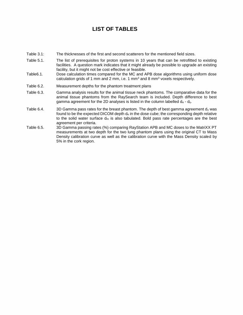
Table 3.1: The thicknesses of the first and second scatterers for the mentioned field sizes.

Table 5.1. The list of prerequisites for proton systems in 10 years that can be retrofitted to existing facilities. A question mark indicates that it might already be possible to upgrade an existing facility, but it might not be cost effective or feasible.

Table6.1. Dose calculation times compared for the MC and APB dose algorithms using uniform dose calculation grids of 1 mm and 2 mm, i.e. 1 mm3 and 8 mm3 voxels respectively.

Table 6.2. Measurement depths for the phantom treatment plans

Table 6.3. Gamma analysis results for the animal tissue neck phantoms. The comparative data for the animal tissue phantoms from the RaySearch team is included. Depth difference to best gamma agreement for the 2D analyses is listed in the column labelled de - dγ.

Table 6.4. 3D Gamma pass rates for the breast phantom. The depth of best gamma agreement dγ was found to be the expected DICOM depth de in the dose cube; the corresponding depth relative to the solid water surface dm is also tabulated. Bold pass rate percentages are the best agreement per criteria.

Table 6.5. 3D Gamma passing rates (%) comparing RayStation APB and MC doses to the MatriXX PT measurements at two depth for the two lung phantom plans using the original CT to Mass Density calibration curve as well as the calibration curve with the Mass Density scaled by 5% in the cork region.

CHAPTER 1: THESIS OVERVIEW AND SCIENTIFIC AND

TECHNICAL CONTRIBUTIONS TO THE FIELD OF PROTON

THERAPY

INTRODUCTION

Wilson first proposed the use of accelerated protons for radiation therapy purposes in 1946 [1.1]

and the first patients were treated with protons in 1954 at the Lawrence Berkeley Laboratory (LBL)

[1.2]. After years of dedicated work from many people in the field of particle radiation therapy [1.3],

we finally reached the stage to declare that proton therapy is now ready for mass adoption in the

clinical practice. In the 19th century, Arthur Schopenhauer (1788-1860) stated that all truth passes

through three stages. First, it is ridiculed, second it is violently opposed, and third it is accepted

as self-evident. It is my opinion that the clinical realization of Pencil Beam Scanning (PBS) [1.4,

1.5] along with many other technological advances, made it possible for proton therapy to

advance to the third stage of Schopenhauer’s hierarchy. We will continue to see a significant

growth in the number of proton therapy treatment vaults over the next few decades if we continue

to develop and implement technologies that will decrease the cost of proton therapy systems,

while increasing proton delivery efficiencies. This notion is supported by the fact that the clinical

realization of PBS allows for the exploitation of the full potential of accelerated proton beams in

the pursuit of increasing the therapeutic ratio. PBS is the generic name for delivering radiation

dose to a target using individually controlled pencil beams of accelerated protons to cover a target

in 3 dimensions (3D). It is my opinion (which is supported by many), that PBS will have a more

significant impact on cancer treatment outcomes than the introduction of IMRT had on x-ray

therapy. Bringing PBS to mass clinical adoption is a true testimony of the importance of the

radiation therapy technology evolution that started with Roentgen’s discovery of x-rays in 1896.

It is also true that the predicted growth in proton utilization will allow for cost and construction time

reductions but at this stage it is still an enormous battle to get a typical proton therapy facility

financed. This means that we cannot only rely on the mass adoption of proton therapy to reduce

costs – basically a catch 22 situation. In Chapter 5 I will argue that we can now exit out of this

conundrum.

As stated above, after many years of development, proton therapy is finally reaching the point of

widespread adoption in clinical practice worldwide. This is mainly due to three contributing factors:

advances in accelerating technology, advances in delivery techniques, and excellent clinical

results [1.6, 1.7, 1.8]. First, technological developments have made proton therapy systems

commercially available and allowed these systems to become more compact and less expensive.

Second, the clinical realization of pencil beam scanning (PBS) has allowed proton therapy to align

with modern day state-of-the-art intensity modulated x-ray radiation therapy (IMRT) treatments.

Thirdly, the widespread adoption of proton therapy that we are experiencing today is fully justified

by early clinical and technical research and developments. The chronology of this development

process is described in this thesis.

The aim of this work is to discuss and document early fundamental developments that I was

involved with since the first patients were treated with protons at the iThemba LABS in Cape

Town, South Africa in 1993 [1.9] and at the Indiana University Health Proton Therapy Center in

Bloomington Indiana, USA in 2004 [1.10]. I will discuss how my early experiences at these

centers enabled me to formulate the technical configuration for ProCure Treatment Centers in an

attempt to make proton therapy available in the community setting through standardization and

cost reduction technologies. I will discuss how this early experience prepared me to participate

and spearhead the developments that are required to further reduce the cost of proton therapy

over the next ten years while increasing the efficiencies that will make proton therapy a financially

viable option for many cancer patients.

OVERVIEW OF THE WORK PRESENTED

In Chapter 1, I provide a short overview of each chapter of the thesis and list the major scientific

and technical contributions that I have made to the field of proton therapy. Most of these

contributions are discussed in the thesis and will be highlighted in the respective sections

Chapter 2 is titled, “Proton Therapy and the Historic Developments that Enabled Proton Therapy

to Become A Major Clinical Tool in Radiation Therapy”. In this chapter, I will discuss the

fundamental physical and clinical principles of proton therapy and the history of proton therapy. I

will also highlight the major hurdles that must be overcome in order to increase the utilization of

proton therapy. The requirements for current, state-of-the-art and future proton therapy systems

will be discussed briefly and reviewed in order to evaluate whether the technological

developments are on the right track. This is an overview chapter that will allow the reader to be

aware of the historical developments that brought proton therapy to the point of mass adoption.

This chapter also sets the scene for the rest of the thesis.

Chapter 3 is titled, “Early Proton Therapy Systems and Important Fundamental Developments in

the Early Days of Proton Therapy”. In this chapter, I will discuss some important early

fundamental developments in proton therapy technologies and more specifically innovative

contributions that I made as well as technologies that I developed while at the iThemba LABS and

the Indiana University Health Proton Therapy Center (IUHPTC). At these two facilities, clinical

proton therapy was delivered using non-commercial, or “homemade”, proton therapy systems.

The chapter will conclude with discussing innovations and technologies that I proposed and

developed while serving as the Senior Vice President of Technology and Chief Medical Physicists

for Procure Treatment Centers (Procure). Procure was founded to reduce the cost of proton

therapy by leveraging cost reduction technologies and standardizing many aspects of proton

therapy. My experiences at iThemba Labs and IUHPTC prepared me to formulate the Procure

technology portfolio that was implemented at four proton therapy centers across the United

States. Several of these developments, such as the Procure patient positioning systems, were

widely adopted in modern proton therapy systems, while other aspects, like the concept of treating

patients in an upright position, is only now gaining traction world-wide.

Chapter 4 is titled, “The Clinical Realization of Pencil Beam Scanning and the Enormous Impact

on the Usability of Protons in Clinical Practice”. In this chapter, I will address the current uses of

Pencil Beam Scanning (PBS) in state-of-the-art clinical proton therapy facilities and the enormous

benefits that the PBS techniques brought to the field of proton therapy. I will discuss Clinical

examples for the most appropriate targets as well as arguments towards proton certainties in

dose deliveries versus the traditional uncertainties. The rationale for using protons in these cases

will also be discussed. With PBS, proton therapy is no longer limited to small, contiguous targets,

but can bring the greatest clinical benefit to larger, distributed, and often more advanced cancers

that can still be treated radically to achieve a cure. These include cancers where the lymph nodes

need to be treated prophylactically or curatively e.g. breast, Head and Neck (H&N), and high-risk

prostate cancers. This chapter is based on a paper that I authored with the medical physics team

at the Provision Center for Proton Therapy in Knoxville (PCPTK), it was published in the Medical

Physics International Journal in 2016.

Chapter 5 is a forward-looking chapter and is titled, “What is Needed in the Next Ten Years to

Allow for the Mass Adoption of Proton Therapy”. In this chapter, I address the need for continued

improvements in proton therapy delivery methods, technologies, and efficiencies. I make the

argument that proton therapy systems can eventually become much less expensive than current

proton systems. Chapter 5 is partly based on a peer reviewed paper that was published in the

British Journal of Radiology (BJR) in 2020 addressing the question of what is needed in the next

10 years from a beam delivery perspective. The paper was an invited contribution to a special

edition of the BJR and had a 4000-word limit which prevented me from including everything that

I believe is needed in the next 10 years. I was asked to only address beam delivery aspects. My

extensive experience in the field of proton therapy and my 28 year battle to make proton therapy

viable has allowed me to pick 8 aspects that I believe are the most important beam delivery aspect

that vendors need to address and bring to market. In chapter 5, I also add a few more aspects

that I believe are needed outside the realm of beam delivery but closely related to it. I do not

address aspects related to treatment planning and clinical indications but focus instead on the

treatment room.

Chapter 6 is titled, “Validating the RayStation Monte Carlo Dose Calculation Algorithms Using

Realistic Phantoms”. In this chapter, I will present recent work validating the Monte Carlo dose

calculation algorithms for protons in real life clinical situations using innovative phantoms. This

chapter is based on two peer reviewed papers that I authored in 2019 with members of the

medical physics team at PCPTK. The paper describes innovative methods that I devised to

validate the Monte Carlo Dose calculation algorithm that was implemented in the RayStation

treatment planning system in 2017. This work demonstrated that while the classical Pencil Beam

dose calculation algorithms are sufficiently accurate for most targets, the Monte Carlo methods

must be used for lung targets and when beam modifying devices such as range shifters and

apertures are inserted in the beam to tailor the dose better. The fundamental physics behind the

dose calculation algorithms and the results of physical measurements that validate the calculated

dose distributions in near realistic circumstances are presented. This work required innovative

thinking in designing the measurements and the phantoms in order to represent the real clinical

scenarios as realistically as far as possible.

Chapter 7 is a short summary and concluding remarks on the work presented in this thesis.

WORK DONE DURING MY PHD REGISTRATION PERIOD AT UCL

I officially registered for my PhD studies at UCL in the fall of 2016. The requirement was to

publish three peer reviewed papers while registered for the PhD program. Three papers were

submitted to peer reviewed journals in 2019 and got accepted for publication. The first two papers

addressed the work I did to commission and validate the Monte Carlo Dose calculation algorithms

implemented in the RayStation treatment planning system for pencil beam scanning proton

therapy systems. This work required the development of innovative phantoms to represent

clinical cases in a realistic manner and is presented in Chapter 6 of this thesis. The references

to the published papers concerning this work are;

Schreuder AN, Bridges DS, Rigsby L, Blakey M, Janson M, Hedrick SG, Wilkinson JB. Validation of the RayStation Monte Carlo dose calculation algorithm using realistic animal tissue phantoms. J Appl Clin Med Phys. 2019 Oct;

20(10):160-171. doi: 10.1002/acm2.12733. Epub 2019 Sep 21.

Schreuder AN, Bridges DS, Rigsby L, Blakey M, Janson M, Hedrick SG, Wilkinson JB. Validation of the RayStation Monte Carlo dose calculation algorithm using a realistic lung phantom. J Appl Clin Med Phys. 2019 Dec; 20(12):127-

137. doi: 10.1002/acm2.12777. Epub 2019 Nov 25.

My work in improving proton therapy efficiencies and cost reduction to make proton therapy

available to more patients continued during the PhD registration period. I focused on the real

changes that are required to achieve this. That work led to an invitation to prepare a paper for a

special edition of the British Journal of Radiology (BJR) addressing the topic of what is needed in

proton therapy in the next ten years from a beam delivery perspective. Writing a paper on this

topic required in-depth research and knowledge of technologies that have been developed but

not implemented or that are being developed and should be implemented over the next ten years.

The peer reviewed invited paper was accepted for publication in October 2019 and published in

the special edition in February 2020. It is presented in Chapter 6 of this thesis. The reference to

this published paper is;

Schreuder AN, Shamblin J. Proton therapy delivery: what is needed in the next ten years? Br J Radiol.

2020 93:1107; Epub 2019 Nov 14:20190359. doi: 10.1259/bjr.20190359. PMID: 31692372

The work I did with respect to the future aspects of proton therapy, other than the beam delivery

aspects discussed in the BJR paper, is also described in Chapter 5 of this thesis. This includes

the efforts towards improving proton therapy efficiencies and the justification of changing the

paradigm in patient position towards treating patients in an upright rather than lying down position.

This work is obviously continuing beyond the PhD project, but a significant amount of research

was done on this topic during the registration period.

CONTRIBUTIONS TO THE FIELD OF PROTON THERAPY

This thesis brings to light a long list of contributions that I personally made to the field of proton

therapy over the last 28 years and addresses future needs in proton therapy in a practical manner.

Many of these contributions were enabled by the opportunities that presented themselves during

the early days of proton therapy developments at the so called “homemade” proton therapy

systems before proton therapy systems became commercially available circa 1995 to 2005.

During the phase when proton therapy systems were not commercially available, it was apparent

that scientists and engineers had to come up with their own solutions to solve problems or to

achieve certain goals. This provided excellent training and development opportunities for

professionals in the field and I benefitted largely from that. I spent endless hours doing beam

measurements and calculations to learn how things work and to devise solutions.

The main areas in which I made noticeable contributions are;

1. Proton dosimetry;

a. The development of the world’s smallest thimble ionization chamber that could be used

for dose measurements in high-dose gradient radiation beams.

b. The development of in-beam energy monitors to measure the proton beam energy prior

to or during beam delivery, also known as the transmission multi-layer ionization

chamber and Aluminum Multilayer Faraday Cup.

c. The development of a water phantom that can position a multi element ionization

chamber at multiple depths in a water phantom to allow for patient specific dose

calibrations in an efficient manner.

d. Development of a quick installation and exchange mechanisms for quality assurance

equipment in the treatment room (not discussed in this thesis).

2. Proton Treatment planning;

a. Development of a 3D proton treatment planning system based on the Voxelplan system.

b. Development of unique near reality phantoms to validate proton dose calculation

algorithms.

3. Beam Delivery;

a. The development and clinical implementation of a unique dual scattering system for a

passive scattering beam delivery system.

b. The proposal of a unique Non-Orthogonal beam treatment room utilizing a concept

where two fixed beamlines shares the same isocenter.

c. The use of ridge filters to increase the efficiency in uniform scanning beam delivery

systems.

4. Patient positioning;

a. The development of unique robotic patient positioners for patient positioning in proton

therapy.

b. The development of a robotic based cone beam CT system.

c. The development of a treatment chair that is attached to a robotic patient positioner to

allow for thoracic and intracranial treatments in the seated position.

d. The development of an inclined CT scanner that allows for fan beam CT (axial) scans

on a patient in any position between lying down and the seated position.

e. The development of a unique optical tracking system based on stereoscopic 2D

cameras to help with patient positioning and motion tracking during treatment (not

discussed in this thesis).

f. The development of a remote anesthesia system to enhance efficiencies in treating

pediatric patients.

5. Training;

a. The development of a unique proton therapy training center and training programs to

decrease the startup time of a proton therapy system while accelerating the full

utilization of such systems.

b. Introducing a training school at the annual international Proton Therapy Cooperative

Group (PTCOG) meetings.

c. Training clinicians in all technical aspects of proton therapy during the startup phases

of 7 new proton therapy facilities.

6. Proton therapy system development and configuration;

a. Developing a unique proton therapy system configuration based on a combination of

Gantry and fixed beams treatment rooms.

b. Commissioning of 9 new proton therapy systems.

Most of the abovementioned contributions are addressed throughout the thesis and will be

highlighted in the respective sections. Many of these contributions are now implemented in

routine clinical practice in many protontherapy centers across the world. I hold three patents in

the field i.e. (1) on the ProCure / Forte patient positioner (2) the Robotic based CBCT system and

(3) a remote anesthesia system.

PUBLICATIONS RELATED TO PROTON THERAPY

I have authored the following papers related to various topics in proton therapy and more

specifically related to the work that I present in this thesis.

4.1 First Author papers

1. Andries N Schreuder, Jacob Shamblin: Proton Therapy delivery: what is needed in the next ten years? Br J Radiol 2019; 92 20190359

2. Schreuder AN, Bridges DS, Rigsby L, Blakey M, Janson M, Hedrick SG, Wilkinson JB; Validation of the RayStation Monte Carlo dose calculation algorithm using a realistic lung phantom. J Appl Clin Med Phys. 2019 Dec; 20(12):127137. doi: 10.1002/acm2.12777.

3. Schreuder AN, Bridges DS, Rigsby L, Blakey M, Janson M, Hedrick SG, Wilkinson JB; Validation of the RayStation Monte Carlo dose calculation algorithm using realistic animal tissue phantoms. J Appl Clin Med Phys. 2019 Oct;20(10):160-171. doi: 10.1002/acm2.12733.

4. A N Schreuder, D T L Jones, J L Conradie, D T Fourie, A H Botha, A Muller, H A Smit, A O'ryan, F J A Vernimmen, J Wilson and C E Stannard. The Non-orthogonal Fixed Beam Arrangement for the Second Proton Therapy Facility at the National Accelerator Centre. CP475, Applications of Accelerators in Research and Industry, Eds J L Duggan and I L Morgan, The American Institute of Physics, (1999) pp 963966

5. A N Schreuder, D T L Jones, J E Symons, E A De Kock, J K Hough, J Wilson, F Vernimmen, W Schlegel, E H Höss an M Lee. The NAC proton treatment planning system. Stralentherapie Onkol. 1999; 175: Suppl II:10-12

6. A N Schreuder, D T L Jones and J E Symons. The quality control program for NAC neutron therapy facility. Advances in Hadrontherapy. Eds. U Amaldi, B Larsson and Y Lemoigne, Elsevier BV, Amsterdam (1997) pp 223-229.

7. A N Schreuder, D T L Jones, J E Symons, E A de Kock, F J A Vernimmen, J Wilson, L P Adams and J K Hough. Three years' experience with the NAC proton therapy patient positioning system. Advances in Hadrontherapy, Eds. U Amaldi, B Larsson and Y Lemoigne, Elsevier BV, Amsterdam (1997) pp 251-258.

8. A N Schreuder, D T L Jones and A Kiefer. A small ionization chamber for dose distribution measurements in a clinical proton beam. Advances in Hadrontherapy, Eds. U Amaldi, B Larsson and Y Lemoigne, Elsevier BV, Amsterdam (1997) pp 284-289.

9. A N Schreuder, D T L Jones, J E Symons, T Fulcher and A Kiefer: The NAC Proton Therapy Beam Delivery System. Proc. 14th Int. Conf. on Cyclotrons and their Applications, Ed. J. Cornell, World Scientific, Singapore (1996) pp491-498.

4.2. Other papers as co-author or senior author.

10. Samantha G. Hedrick, Marcio Fagundes, Ben Robison, Marc Blakey, Jackson Renegar, Mark Artz, Niek Schreuder: A comparison between hydrogel spacer and endorectal balloon: An analysis of intrafraction prostate motion during proton therapy. Journal of Applied Clinical Medical Physics 02/2017; 18(2).

11. Samantha G. Hedrick, Marcio Fagundes, Sara Case, Jackson Renegar, Marc Blakey, Mark Artz, Hao Chen, Ben Robison, Niek Schreuder: Validation of rectal sparing throughout the course of proton therapy treatment in prostate cancer patients treated with SpaceOAR®. Journal of Applied Clinical Medical Physics 01/2017; 18(1):8289.

12. Yuanshui Zheng, Yixiu Kang, Omar Zeidan, Niek Schreuder: An end-to-end assessment of range uncertainty in proton therapy using animal tissues. Physics in Medicine and Biology 10/2016; 61(22):8010-8024.

13. Ding X, Zheng Y, Zeidan O, Mascia A, Hsi W, Kang Y, Ramirez E, Schreuder N, Harris B., A novel daily QA system for proton therapy. J Appl Clin Med Phys. 2013 Mar 4;14(2):4058.

14. Zheng Y, Liu Y, Zeidan O, Schreuder A N, Keole S., Measurements of neutron dose equivalent for a proton therapy center using uniform scanning proton beams. Med Phys. 2012 Jun; 39(6):3484-92.

15. Zheng Y, Ramirez E, Mascia A, Ding X, Okoth B, Zeidan O, Hsi W, Harris B, Schreuder A N, Keole S., Commissioning of output factors for uniform scanning proton beams. Med Phys. 2011 Apr; 38(4):2299306.

16. Farr JB, O'Ryan-Blair A, Jesseph F, Hsi WC, Allgower CE, Mascia AE, Thornton AF, Schreuder A N, Validation of dosimetric field matching accuracy from proton therapy using a robotic patient positioning system. J Appl Clin Med Phys. 2010 Apr 12;11(2):3015.

17. Hsi WC, Moyers MF, Nichiporov D, Anferov V, Wolanski M, Allgower CE, Farr JB, Mascia AE, Schreuder A N., Energy spectrum control for modulated proton beams. Med Phys. 2009 Jun; 36(6):2297-308.

18. Hsi WC, Schreuder A N, Moyers MF, Allgower CE, Farr JB, Mascia AE., Range and modulation dependencies for proton beam dose per monitor unit calculations. Med Phys. 2009 Feb;36(2):634-41.

19. Farr JB, Mascia AE, Hsi WC, Allgower CE, Jesseph F, Schreuder A N, Wolanski M, Nichiporov DF, Anferov V., Clinical characterization of a proton beam continuous uniform scanning system with dose layer stacking. Med Phys. 2008 Nov; 35(11):4945-54.

20. Nichiporov D, Solberg K, Hsi W, Wolanski M, Mascia A, Farr J, Schreuder A., Multichannel detectors for profile measurements in clinical proton fields. Med Phys. 2007 Jul; 34(7):2683-90.

21. Allgower CE, Schreuder A N, Farr JB, Mascia AE., Experiences with an application of industrial robotics for accurate patient positioning in proton radiotherapy. Int J Med Robot. 2007 Mar; 3:72-81. Review.

22. Kim A, Kim J, Insik H, Schreuder N, Farr J; Simulations of Therapeutic Proton Beam Formation with GEANT4. Journal of the Korean Physical Society, 47(2), 2005, 197-201.

23. J. Katuin, N. Schreuder, The Use of Industrial Robot Arms for High Precision patient Positioning.

Proc. CAARI 2002, Denton TX, Nov. (2002)

24. V. Anferov, B. Broderick, J.C. Collins, D.L. Friesel, D. Jenner, W.P. Jones, J. Katuin, S.B. Klein, W. Starks, J. Self, N. Schreuder, The Midwest Proton Radiation Institute Project at the Indiana University Cyclotron Facility. Cyclotrons and their Applications, AIP 600 pp27-29 (2001).

25. D T L Jones and A N Schreuder. Magnetically scanned proton therapy beams: rationales and principles. Radiation Physics and Chemistry 61 (2001) 615-618

26. J Gueulette, L Böhm, J P Slabbert, B M De Coster, G S Rutherfoord, A Ruifrok, M OctavePrignot, P J Binns, A N Schreuder, J E Symons, P Scalliet and D T L Jones, Proton relative biological effectiveness (RBE) for survival in mice after thoracic irradiation with fractionated doses. Int. J. Radiat. Oncol. Biol. Phys. 47 (2000), 1051-1058.

27. J Gueulette, L Böhm, B De Coster, S Vynckier, M Octave-Prignot, A N Schreuder, J E Symons , D T L Jones, A Wambersie and P Scalliet. RBE variation as a function of depth in the 200 MeV proton beam produced at the National Accelerator Centre. Radiother. Oncol. 42 (1997) 303-309.

28. J Gueulette, B M De Coster, V Gregoire, P Scalliet, A Wambersie, J P Slabbert, L Böhm, P J Binns, E A de Kock, A N Schreuder, J E Symons and D T L Jones. RBE of the 200 MeV proton beam produced at the National Accelerator Centre of Faure (RSA) for late lung tolerance in mice

after single and fractionated irradiation (preliminary results). Advances in Hadrontherapy, Eds. U Amaldi, B Larsson and Y Lemoigne, 1997, Elsevier BV, Amsterdam (1997) pp 413 - 419.

29. E A de Kock and A N Schreuder. Comments on the calibration of CT Hounsfield units for radiotherapy treatment planning. Phys. Med. Biol. 41 (1996) 1524-1526.

30. D T L Jones, A N Schreuder and J E Symons: Particle Therapy at NAC. Physical Aspects Proc. 14th Int.Conf. on Cyclotrons and their Applications, to be published by World Scientific

31. D T L Jones, A N Schreuder, J E Symons, H Ruther, G Van der Vlugt, K F Bennet and A D B Yates. Use of Stereophotogrammetry in Proton Radiation Therapy. Proc. Int. Fig Symposium, Cape Town, 1995, ed. H Ruther, Univ.of Cape Town, 1995, P138-152)

32. D T L Jones, A N Schreuder, J E Symons and M Yudelev: The NAC Particle Therapy Facilities. Hadrontherapy in Oncology. (1994) 307

SUMMARY

This thesis summarizes the work that I have done in proton therapy over the last 28 years. It

highlights the chronological developments that allowed me to make contributions in the field of

proton therapy. The thesis also provides a look into the future, explaining the need for changing

the paradigms towards patient positioning to allow for treating patients in the upright position.

This major paradigm change is required to bring all the clinical benefits of proton therapy to many

more cancer patients worldwide and will open the doors for other ion species to be used in cancer

therapy. Chapter 2 provides a chronology of historic developments in proton therapy while chapter

3 describes the work I did at the earlier stages of my career that have allowed me to make

significant contributions to the field. Chapter 4 describes the benefits of PBS and the enormous

impact the clinical realization of PBS had on the proliferation of proton therapy worldwide. The

work done specifically during the PhD registration period is captured in chapters 5 and 6

describing the future aspects of proton therapy and the scientific work towards validating the

RayStation Monte Carlo Dose calculation algorithms.

CHAPTER 2:

PROTON THERAPY AND THE HISTORIC DEVELOPMENTS THAT

ENABLED PROTON THERAPY TO BECOME MAJOR CLINICAL TOOL

IN RADIATION THERAPY.

1. INTRODUCTION

In this chapter, I will discuss the history of proton therapy and the hurdles that were necessary to

overcome in order to increase the utilization of proton therapy. This is an overview chapter that

will set the scene for the rest of the thesis.

After many years of development, proton therapy is finally reaching the point of widespread

adoption in clinical practice worldwide [2.1]. This is mainly due to three contributing factors:

• advances in accelerating technology,

• advances in beam delivery techniques and

• excellent clinical results.

Firstly, technological developments have made proton therapy systems commercially available

and allowed these systems to become much more compact and less expensive. Secondly, the

clinical realization of pencil beam scanning (PBS) has allowed proton therapy to be more in-line

with modern day, state-of-the-art, intensity modulated x-ray radiation therapy (IMRT) treatments.

PBS is the generic name for delivering radiation dose to a target using individually controlled

pencil beams of accelerated protons to cover a target in 3 dimensions (3D). Thirdly, the

widespread adoption of proton therapy that is now happening is fully justified on the basis of early

clinical and technical research and developments.

2. PROTON RADIATION THERAPY

The goal of radiation therapy has always been to increase the therapeutic ratio, which is defined

as the ratio between tumor control and normal tissue complications [2.2]. This means that if tumor

control is increased while reducing treatment related complications, the therapeutic ratio can be

increased. The primary means of reducing complications is by reducing the dose outside the

target volume. Therefore, external beam radiation therapy technology improvements always

aimed at getting a higher dose at depth. In external beam proton radiation therapy, the protons

are used in a similar fashion to x-rays in that multiple beams are aimed at the target; however,

with proton beams, the radiation stops at the distal end of the target area. This means that for a

specific beam, no dose is delivered beyond the target. In addition, when proton beams of

decreasing energy are stacked on top of each other, the primary pristine Bragg peaks are spread

out in the beam direction, forming the Spread Out Bragg Peak (SOBP), which has a higher dose

at depth than at the entrance, illustrated in figure 2.1.

Figure 2.1. Depth dose curves for an 8 MV x-ray beam (Dash-dot-dot line) and a 200 MeV proton beam (solid lines). The thinner solid lines show Bragg peaks for proximal energy layers stacked onto the deepest energy layer to constitute the Spread-Out Bragg Peak (Dashed line) required to cover the target area (shaded).

3. HISTORY OF PROTON RADIATION THERAPY

3.1 Physics:

Three pioneers in the history of physics deserve special mention when we review the history of

proton therapy. They are Ernest Rutherford, William Bragg and Ernest Lawrence. Rutherford’s

work on the atomic model led to the discovery of the proton when the nucleus of a hydrogen atom

was first called a proton in 1920 [2.3]. During the same time period, Bragg postulated that a

charged particle entering a medium will have a definite range and will lose more energy towards

the end of its range, hence the name Bragg Peak for the depth dose curve of a charged particle

[2.4]. The invention of the cyclotron by Lawrence made high energy protons available to the field

of particle therapy.

3.2 Accelerators:

Lawrence built the first cyclotron in 1931 to prove the principle which led to the construction of

several, higher energy cyclotrons used in many pioneering physics experiments. Of special

interest for proton therapy was the construction of the 184-inch cyclotron at the Berkeley National

laboratory that was used for the world’s first particle therapy treatments [2.5]. The evolution of

cyclotrons is illustrated in figure 2.2 which shows the acceleration diameter in inches and energy

in MeV against the year the cyclotron was built.

Figure 2.2: The evolution of cyclotrons. The acceleration diameter (Blue bars) in inches and energy in MeV (red line) is illustrated against the year the cyclotron was built.

The Manhattan project, that was started by the USA government to develop the atomic bomb,

had a major impact on scientific developments in the thirties and forties. Robert Wilson, who

received his doctorate under the supervision of Lawrence for his work on the development of the

cyclotron at Berkeley, became the head of the cyclotron group and later the research division of

the Manhattan project in 1943. The Calutrons that were used at the Oakridge facility in Knoxville

to enrich uranium for the atomic bomb are basically a half cyclotron and were developed based

on the knowledge gained from developing the cyclotron. Wilson’s involvement in the Manhattan

project motivated him to focus his energy on peaceful uses of his knowledge.

3.3 First Proton Radiation Therapy:

In 1946, Wilson published a paper [2.6] in which he claimed that the properties of fast proton

beams made it, “possible to irradiate intensely a strictly localized region within the body, with but

little skin dose”. In addition, he also claimed that, “it will be possible to treat a volume as small as

1.0 cc anywhere in the body and to give that volume several times the dose of any of the

neighboring tissue”. These claims and ideas, although many years ahead of the technology in the

1940’s, have proven tremendously influential to charged particle therapy.

In 1954, the first patient was treated with a proton beam at the Lawrence Berkeley laboratory

(LBL) California, USA [2.7, 2.8, 2.9] for a non-malignant condition. Shortly after, in 1957, Uppsala

University adapted their 185 MeV proton cyclotron for clinical purposes, and soon after treated

their first cancer patient [2.10, 2.11, 2.12]. The development of proton therapy gained slow

momentum during the sixties and seventies, with pioneering work done primarily at the Harvard

Cyclotron laboratory in Cambridge, Massachusetts (USA) and at LBL.

In a paper that Wilson wrote in 1946, he proposed capitalizing on the fact that protons stop at the

target in the patient’s body as illustrated in figure 2.3 – panel A. However, due to a lack of density

information inside the patient’s body, it was not possible to calculate the stopping point of the

protons with any degree of accuracy. This led to the use of the so-called shoot-through technique

as illustrated in figure 2.3 – Panel B [2.13]. The shoot-through technique was primarily used for

intracranial treatments where the beam energy was high enough to go through the patient’s body

with the protons stopping on the other side of the patient’s body in a stopping block or the wall of

the treatment room. Setting the patient up for the shoot-through technique was fairly easy using

in-line x-ray beams. The lack of treatment planning computers was another reason for using the

shoot-through technique. Panel C, in figure 2.3, shows a typical shoot-through plan for a pituitary

gland target treated at the iThemba LABS circa 1995 using a 5-field shoot-through plan [2.14].

Figure 2.3. A schematic illustration of the first utilization of protons. Panel A shows using the Bragg peak as proposed by Wilson while panel B shows how the first treatments were done using the shoot through technique. Panel C shows a shoot through plan on a patient treated for a Pituitary lesion using the shoot through technique.

3.4 The CT Scanner:

The lack of density information inside the patient’s body was only overcome when the CT Scanner

was invented by Sir Godfrey Hounsfield and Allan Cormack [2.15, 2.16, 2.17]. The first EMI-CT

Scanner was installed in Atkinson Morley Hospital in Wimbledon, England, and the first patient

brain-scan was done on 1 October 1971 [2.18]. Hounsfield and Cormack shared the Nobel prize

for this invention in 1979 [2.19, 2.20].

3.5 3D treatment planning:

Pioneering work by Goitein et al. at Massachusetts General Hospital in Boston led to what I

believe was the world’s first 3D treatment planning system based on CT data [2.21, 2.22]. The

concept of the digitally reconstructed radiograph (DRR) was introduced by them to visualize the

beam trajectory through the patient’s body for treatment planning and for setup purposes. The

3D treatment planning system developed by Goitein finally led to the full use and exploitation of

the proton Bragg Peak being spread out across the target and stopping at the distal end of the

target. Two very commanding figures from Goitein’s paper in 1983 are shown in figure 2.4. Panel

A, in figure 2.4, shows the geometry involved to calculate the beam’s eye view of anatomical

structures that is used to avoid certain anatomical structures on the way to the target i.e. beam

angle selection. Panel B shows the concept of the DRR that is used for setup. The use of both

of these concepts are still instrumental in modern day radiation therapy.

Figure 2.4: Excerpts from Goitein’s 1983 paper illustrating the concepts of the Beam’s eye view and the DRR.

3.6 Treatment planning dose calculation algorithms:

Using protons to treat a target has always been a 3-dimensional problem. Unlike photon therapy,

where the distribution of dose is less impacted by density variations along the beam path, it was

never possible to adequately extrapolate the dose from one anatomical plane in the patient’s body

to another as was done in the early days of photon treatment planning. It was always necessary

to calculate the dose in multiple planes through the target region using the density information

along the plane. These calculations required a fair amount of computing power and it was not

until the 1980s that computers became available that could use the CT data as mentioned earlier

to do advanced 3D dose calculations in the patient’s body. The early dose algorithms used ray-

tracing algorithms that addressed the problem in a simplistic 2D fashion [2.13]. To calculate the

dose at a certain point in the patient’s body, the pixel density along a ray-line, starting at the

effective source position, was summed to obtain the total cumulative density that the protons have

to traverse to reach that point. This included the compensator material and any other materials

in the beam path, such as immobilization devices, while beam delivery components, such as the

transmission ionization chambers and scatterers, were excluded since they were accommodated

in the pristine beam range definition. The dose at the specific depth was simply obtained from a

lookup table containing measured depth dose data. The impact of the aperture that was inserted

to shape the lateral extent of the beam was obtained from a profile function or a lookup table that

modelled or listed the dose as function of distance from the aperture edge at different depths in

water. It is clear that these ray-trace algorithms were not able to accommodate multiple coulomb

scattering in the patient, however it was able to correct for density differences along the beam

path to a reasonable degree of accuracy.

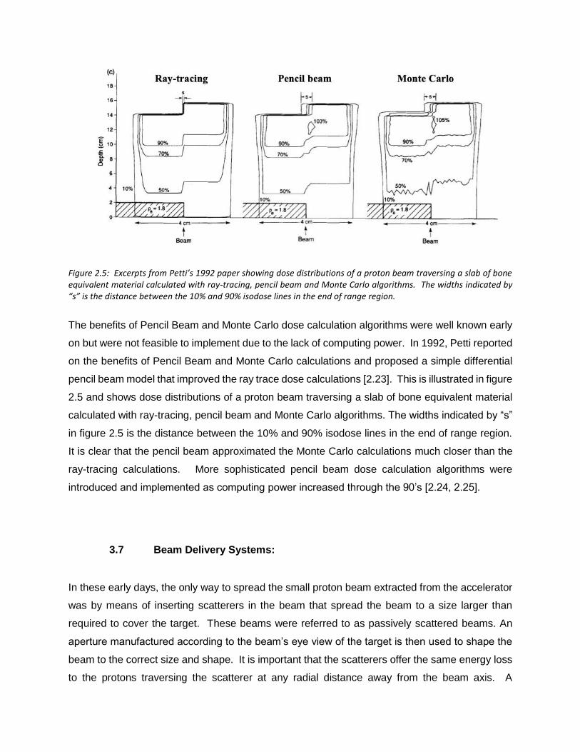
Figure 2.5: Excerpts from Petti’s 1992 paper showing dose distributions of a proton beam traversing a slab of bone equivalent material calculated with ray-tracing, pencil beam and Monte Carlo algorithms. The widths indicated by “s” is the distance between the 10% and 90% isodose lines in the end of range region.

The benefits of Pencil Beam and Monte Carlo dose calculation algorithms were well known early

on but were not feasible to implement due to the lack of computing power. In 1992, Petti reported

on the benefits of Pencil Beam and Monte Carlo calculations and proposed a simple differential

pencil beam model that improved the ray trace dose calculations [2.23]. This is illustrated in figure

2.5 and shows dose distributions of a proton beam traversing a slab of bone equivalent material

calculated with ray-tracing, pencil beam and Monte Carlo algorithms. The widths indicated by “s”

in figure 2.5 is the distance between the 10% and 90% isodose lines in the end of range region.

It is clear that the pencil beam approximated the Monte Carlo calculations much closer than the

ray-tracing calculations. More sophisticated pencil beam dose calculation algorithms were

introduced and implemented as computing power increased through the 90’s [2.24, 2.25].

3.7 Beam Delivery Systems:

In these early days, the only way to spread the small proton beam extracted from the accelerator

was by means of inserting scatterers in the beam that spread the beam to a size larger than

required to cover the target. These beams were referred to as passively scattered beams. An

aperture manufactured according to the beam’s eye view of the target is then used to shape the

beam to the correct size and shape. It is important that the scatterers offer the same energy loss

to the protons traversing the scatterer at any radial distance away from the beam axis. A

compensator is used to modify the energy of the protons that pass through the aperture in such

a manner that the protons stop at the distal end of the target. The compensator combines the

effects of inhomogeneities in the beam path and the fact that the distal edge of the target varies

across the beam area [2.26, 2.27]. This technique is essentially three-dimensional (3D) conformal

proton therapy. Although passive scatter techniques decreased the integral dose, i.e. the dose

outside the target, dramatically, they still suffered from inadequate dose conformity, secondary

dose from neutrons, and heavy apertures and compensators that remained problematic. I played

an integral role in developing two traditional proton therapy systems during the earlier parts of my

career in proton therapy. The technical aspects of the design and operation of these two systems,

i.e. the proton therapy facility at the iThemba Laboratories (iThemba LABS) in Cape Town, South

Africa [2.28] and the Indiana University Health Proton facility (IUHPTC) in Bloomington, IN, USA

[2.29] is discussed in chapter 3 of this thesis.

Pencil beam scanning (PBS), first proposed by Kanai in 1980 [2.30], made it into clinical practice

when the first proton patients were treated with PBS at the Paul Scherer institute in Switzerland

in 1996 [2.31, 2.32]. Whereas early proton treatment systems relied on spreading the beam and

then shaping it through the use of patient specific apertures and compensators, PBS actively

controls a small pencil beam, steering it to deliver dose in discrete “spots” allowing the treatment

of larger and non-contiguous targets. It took the industry many years to commercialize PBS

technologies and make it available to more facilities. Today, PBS is in routine clinical use in most

proton therapy facilities around the globe. PBS allows for full intensity modulated proton therapy

(IMPT) where the target dose can be optimized over all the beams. IMPT became a clinical reality

in many more treatment centers since 2010, when the Hitachi system at MD Anderson and the

IBA system at UPenn started treating patients with PBS. The increased flexibility in dose shaping

has enabled improved dose conformation, especially to large and non-contiguous targets, and

truly revolutionized proton therapy in the last few years. The general utilization of proton therapy

has been expanded to almost all sites in the body [2.33, 2.34, 2.35, 2.36] and with robust

optimization [2.37], which is a practical solution only with PBS, the traditional problems with range

uncertainties have been addressed to a greater extent. Using intelligent optimization strategies

and computer algorithms, treatment plans are now optimized with the perceived uncertainties in

mind, rendering the delivered plans consistent against changes and uncertainties in the entire

treatment process. Certainties, rather than uncertainties, in PBS proton beam delivery, can be

considered, and this provides physicians with vastly improved confidence in the delivered target

dose. The largest paradigm shift caused by PBS is that clinicians are now faced with the question

of which targets will not benefit from proton therapy. Traditionally, the inverse question was asked

when the proton dose distributions were less conformal and the benefits in protons mainly came

from the reduced integral dose.

Similar to the x-ray therapy evolution from 3D conformal treatments to intensity modulated

radiation therapy (IMRT) and eventually arc therapy (VMAT, Tomotherapy and rapid Arc),

intensity modulated proton therapy (IMPT) using PBS offered treatment improvements over 3D

conformal proton therapy. PBS offers much lower integral dose than traditional x-ray therapy and

often more conformal dose distributions for a myriad of cancer types when compared to x-rays

and even 3D proton therapy. The quest for further technological developments is therefore fully

supported by the cancer therapy technological advances over the past century.

4. PROTON THERAPY TODAY AND THE YEARS AHEAD.

Recent advances in the proton therapy industry are changing the way the technology is used.

New techniques in beam delivery, treatment planning, dose calculations, and image guidance are

improving the quality of treatments for current treatment sites and opening the door for sites not

previously treated with protons. As stated before, the most significant advancement in recent

years have been the widespread adoption of PBS delivery techniques. These developments

impacted the wider adoption of proton therapy world-wide.

The introduction of Monte Carlo (MC) dose calculation algorithms into clinical routine was another

important milestone in the delivery of proton beam therapy [2.38, 2.39]. This allowed for more

accurate dose calculation of complex targets such as breast, bi-lateral head & neck, and lung

targets. It also allowed for the use of beam shaping devices such as range shifters, ridge filters,

and apertures to be used with PBS. The testing and validation of MC dose calculation algorithms

confirmed the accuracy and validity of using MC calculations in all treatment sites [2.40, 2.41]

The past experiences and developments in proton therapy as discussed earlier in this chapter

allowed for many technologies to be developed across the world by many research institutions

and industry sponsored grants. Unfortunately, many of these developments never made it into

clinical practice to date but matured to such an extent that they can and should be implemented

over the next few years [2.42].

The cost effectiveness of proton therapy systems remains a major challenge for the industry.

Many vendors entered the field of particle therapy producing systems that mimics x-ray therapy

systems in many regards, i.e. based on rotating gantry structures that allows for rotating the beam

around the patient lying on a treatment couch. These systems are very large and require very

large shielded bunkers which are expensive and take a long time to construct and to commission

for clinical use. Proton therapy also requires more manpower to prepare and to deliver to the

patient. These aspects can be addressed by changing the paradigm of beam delivery away from

the traditional x-ray-based techniques, i.e. rotating gantries and going back to where radiation

therapy began, i.e. rotating the patient in a fixed beam [2.43]. This allows for the shielded volume

to reduce in size, faster construction and commissioning times, and enhanced efficiencies.

5. SUMMARY

The historical developments that led to Wilson’s proposal to use protons for radiation therapy

treatments and the subsequent developments that enabled proton therapy to become a major

tool in radiation therapy were discussed in this chapter. I joined the field of particle therapy in

1988 when I started working at the iThemba LABS facility in South Africa and assisted in the first

neutron therapy treatments at that facility in September of 1989. In 1990, we started developing

the proton therapy beam line at the facility where the first patients were treated in April 1993. This

means that I joined the proton therapy journey just after the halfway mark and started making

contributions to the field. The rest of the thesis will discuss these contributions.

CHAPTER 3:

EARLIER PROTON THERAPY SYSTEMS AND IMPORTANT

FUNDAMENTAL DEVELOPMENTS

INTRODUCTION

This chapter will discuss some important fundamental early developments in proton therapy

technologies and more specifically, work that I was involved with and initiated at the iThemba

LABS and the Indiana University Cyclotron facility (IUCF), where clinical proton therapy was done

using non-commercial, often referred to as “homemade”, proton therapy systems. The IUCF

facility was first named the Midwest Proton Therapy Institute (MPRI) and later called the Indiana

University Health Proton Therapy Center (IUHPTC). The IUHPTC ceased operations in

December 2014, when it was decided by the IU authorities that it was not feasible to replace the

cyclotron which was built in 1972, with another proton accelerator. The iThemba LABS facility

ceased operations in December 2018 when the medical radiation program was closed due to a

lack of patient referrals to both the neutron and proton facilities. Several of my inventions and

developments at both of these facilities, e.g. patient positioning systems using commercial robots

and dosimetry devices and techniques, are widely adopted and are used in modern proton

therapy systems.

1. PROTON THERAPY AT ITHEMBA LABS

The iThemba Laboratory for Accelerator Based Sciences (iThemba LABS), formerly known as

the National Accelerator Center (NAC) in South Africa was constructed as a national resource to

address three main needs in the country, i.e. basic physics research, isotope production, and

medical radiation. Construction of the facility started in 1978 and the first beam was extracted

from the 200 MeV open sector cyclotron in 1985. The medical radiation division was initially

supposed to have three neutron treatment rooms where patients could be treated with high energy

(fast) neutrons. However, only one isocentric neutron gantry was installed and the first neutron

patients were treated in September 1989 [2.14, 3.1]. It was soon realized that neutron therapy

would not live up to its promises in terms of tumor control since the lack of conformance of the

high LET radiation to the target area was causing more co-lateral harm than was required to

improve the therapeutic ratio [3.2]. The emphasis therefore started to swing towards proton

therapy. In 1990, the first high energy proton Bragg peak in the southern hemisphere was

measured in the neutron therapy room when the first bending magnet in the 360 degree isocentric

neutron gantry was disabled and the beam was extracted through a port in the magnet and

transported horizontally through air to the neutron isocenter. I was personally responsible for

setting up and doing these measurements under the supervision of Dr. Dan Jones who was the

department head. Dr. Dan Jones made exceptional contributions to the field of particle therapy

through serving on many international scientific panels and publishing many research papers

while providing leadership to the iThemba LABS particle therapy programs. The development of

the iThemba LABS proton therapy facility began in all sincerity around June 1990 and I played a

large role in this development.

1.1 The Radiation surgery beamline

The proton therapy beam delivery system was initially designed for radiosurgery purposes only

and the first patient was treated in the iThemba LABS radiosurgery proton therapy beamline in

April 1993 [2.28]. A schematic drawing of the proton beam line is shown in Figure 3.1.

Figure 3.1: A schematic layout of the NAC fixed horizontal beamline that was initially designed for radio surgery purposes only.

Unique features of iThemba LABS fixed beam line design were;

It had a very large throw i.e. the distance between the isocenter and the vacuum window, of

approximately 7 meters since we wanted to spread the beam as much as possible without having

to scatter and flatten the beam much.

It used the “shoot through” treatment technique. This means that the plateau region of the Bragg

peak was used to treat the patient.

It used an occluding ring system to flatten the beam.

It employed a double feedback loop to control the beam position at isocenter.

It used a unique multi-layer ionization chamber (MLIC) to monitor the incident beam energy utilizing

the unwanted halo beam that needed to be stopped anyway.

It used a Multi-layer faraday cup (MLFC) to characterize the energy spread in the beam,

It used a unique stereo photogrammetry patient positioning system to place the target at isocenter

and to monitor any patient motions during treatment.

It used a unique patient positioner that could convert between a chair for seated treatments and a

bed for supine, prone, or decubitus treatments.

It used a unique system to allow for rapid installation of the water phantom for physics QA.

Most of these unique features carry some relevance to modern day systems that will be discussed

briefly in the following sections.

1.2 Large Throw Design

When designing gantry beam delivery systems, a large throw is not possible since the radius of

the gantry must always be optimized to be as small as possible to reduce the shielded volume.

However, when a fixed beamline is used, a large throw can be used to help with beam spreading

and beam diagnostics. A very small angle of deflection of the beam can facilitate a large field at

isocenter. This in turn, will reduce the cost of the scanning magnet and will allow for fast scanning.

The use of fixed beams in the future to reduce facility costs will be discussed in Chapter 5 of this

work. The iThemba LABS radiosurgery proton therapy beamline had a 7 meter throw i.e. the

distance between the vacuum window at the exit of the beamline and the isocenter, as illustrated

in Figure 3.1. The cyclotron was able to accelerate protons to a maximum energy of 200 MeV.

The theoretical maximum range of a 200 MeV proton in water is 25.96 cm [3.3]. The maximum

range measured in the radio surgical beamline at the 50% dose point distal to the Bragg peak

was 24 cm which means that the total energy loss in the large throw beam delivery nozzle was

approximately 2 cm of range in water or 9 MeV. The 7 meters of air accounted for approximately

a 5 MeV energy loss.

1.3 The Shoot thru treatment technique

Shooting the proton beam through the patient’s body does not seem to be very elegant but it is a

technique that is receiving some thought again in modern day particle radiation therapy. The

reason for using the shoot through technique at the iThemba LABS facility was mainly two-fold.

First, the treatment planning for this kind of radiation is simple. Secondly, it is an effective way

that protons can be used for very small radiosurgery lesions. To use this technique, one needs

a very high beam energy or be limited to brain lesions. The 200 MeV proton beam from the

iThemba LABS cyclotron open sector cyclotron limited this method to be used for intracranial

lesions only. The maximum range from a 200 MeV proton beam is approximately 26 cm [3.3]

which is sufficient to traverse any adult patient’s skull. The practically achievable range is less,

due to energy loss in air and certain beam line components. Furthermore, having the proximal

slope of the Bragg peak, where the dose typically increases rapidly in the patient’s body, is not

desirable.

The iThemba LABS beamline used an occluding ring system [3.4] to flatten the beam in order to

minimize the energy loss along in the beam delivery nozzle. The measured depth dose curves

for different field sizes are shown in Figure 3.2. As can be seen from Figure 3.2 the fact that the

Bragg peak to entrance dose ratio decreases as the field size decrease is a great help with

reducing the exit dose. This decrease is due to the loss of transverse electronic equilibrium as a

result of multiple Coulomb scattering. Once a proton scatters out of a narrow proton beam, there

are not enough neighboring beams that can scatter in the opposite direction to replace the proton

that was lost, hence the decrease in fluence which increases with depth in a medium. Small radio

surgical lesions treated typically use field sizes in the range of 10 to 15 mm in diameter with the

lesion at an average depth of 12 cm. This means that the percentage depth dose (%DD) for such

treatments are near perfect – almost 100% at the depth of interest while the penumbra is between

4 and 6 mm as can be seen in Figure 3.3 [2.28].

Figure 3.2. The measured depth dose curves for different field diameters (cm) see ref [2.28].

1.4. The beam delivery nozzle

The detailed characteristics of the iThemba LABS fixed beam delivery nozzle have been

described previously [2.28, 3.5]. The proton beam exited the vacuum 7 meters from the isocenter.

The beam was controlled by two feedback loops. The first beam position monitor was located

just downstream of the vacuum window and consisted of a unique Multi wire ionization chamber

(MWIC) that I designed and described in the paper discussing the characteristics of the fixed

beamline [2.28].

Figure 3.3. The penumbra for the NAC radiosurgery beam as a function of depth.

The beam position, obtained from the MWIC, was fed back to a set of X Y steering magnets a

few meters upstream of the vacuum window. The second steering loop obtained the beam

position from the quadrant ionization chambers installed near the treatment isocenter. The beam

position stability is crucial when using an occluding ring system to spread the beam, hence the

double feedback loop. The occluding ring system is the only design that will allow for spreading

the beam without degrading the beam energy, but it is a very inefficient method. The occluding

ring beam spreading system consisted of a central plug of brass that stops the central core of the

beam [3.4]. A ring of brass of the same thickness as the center plug is mounted concentric to the

plug. This means that most the protons are stopped in the plug and ring. The plug and the ring

are mounted on a 1 mm thick brass plate that spreads the beam that passes through the gap

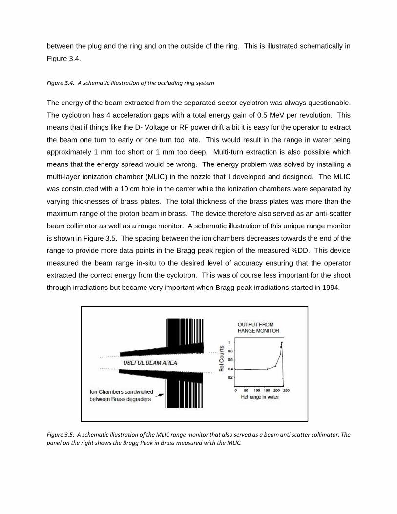
between the plug and the ring and on the outside of the ring. This is illustrated schematically in

Figure 3.4.

Figure 3.4. A schematic illustration of the occluding ring system

The energy of the beam extracted from the separated sector cyclotron was always questionable.

The cyclotron has 4 acceleration gaps with a total energy gain of 0.5 MeV per revolution. This

means that if things like the D- Voltage or RF power drift a bit it is easy for the operator to extract

the beam one turn to early or one turn too late. This would result in the range in water being

approximately 1 mm too short or 1 mm too deep. Multi-turn extraction is also possible which

means that the energy spread would be wrong. The energy problem was solved by installing a

multi-layer ionization chamber (MLIC) in the nozzle that I developed and designed. The MLIC

was constructed with a 10 cm hole in the center while the ionization chambers were separated by

varying thicknesses of brass plates. The total thickness of the brass plates was more than the

maximum range of the proton beam in brass. The device therefore also served as an anti-scatter

beam collimator as well as a range monitor. A schematic illustration of this unique range monitor

is shown in Figure 3.5. The spacing between the ion chambers decreases towards the end of the

range to provide more data points in the Bragg peak region of the measured %DD. This device

measured the beam range in-situ to the desired level of accuracy ensuring that the operator

extracted the correct energy from the cyclotron. This was of course less important for the shoot

through irradiations but became very important when Bragg peak irradiations started in 1994.

Figure 3.5: A schematic illustration of the MLIC range monitor that also served as a beam anti scatter collimator. The panel on the right shows the Bragg Peak in Brass measured with the MLIC.

Multi turn extraction of the beam from the cyclotron not only resulted in the incorrect beam energy

arriving at the treatment room, but also the incorrect energy spread resulting in a broader pristine

Bragg peak. I designed a Multi-Layer Faraday Cup (MLFC) to address that problem. Gottschalk

first demonstrated the use of a MLFC at the Harvard Cyclotron Laboratory (HCL) [3.6]. The

operating principle of a Faraday cup is very simple. When a charged particle stops in an electrical

conductor, the conductor will be charged with an electrical charge equivalent to the charge of the

particle stopping. When such a conductor is connected to an electrical circuit, the charge will flow

from the conductor typically to a ground potential and can be measured with an electrometer. The

charge of a proton is very well known as +1.602 × 10-19 Coulombs which means that if we measure

the charge build up in a faraday cup because of protons stopping in the faraday cup, we are

effectively counting the protons. A MLFC operates in the same way except that the charges in

each of the layers of the MLFC are collected independently. A MLFC therefore counts the number

of protons stopping in each layer of the MLFC. The output from the MLFC can be used to measure

the energy and the energy spread of the beam.

I first built a brass MLFC in the same fashion as the MLIC described above and installed it higher

upstream in the beamline with a smaller hole in the MLFC to collimate the smaller beam in front

of the range modulator. The MLFC used 30, one mm thick brass plates insulated from each other

using 80 µm Kapton foils. The MLFC worked very well to measure the beam range but could not

give reliable energy spread information since the peak is distributed over only 5 channels. A

picture of the brass MLFC and anti-scatter small collimator is shown in Figure 3.6.

Figure 3.6: A picture of the brass MLFC and anti-scatter small collimator

I solved the energy spread problem by developing an Aluminum multi-layer faraday cup (MLFC).

The Al MLFC was constructed using thirty 0.65 mm thick pure Al plates electrically insulated from

each other by 80 µm thin Kapton foils. This allowed for the protons to stop and be recorded in at

least 13 channels, since the density of Al (2.7 g/cm³) is about 3.2 times less than that of Brass

(between 8.4 to 8.73 g/cm³) and I used thinner Al layers. A picture of the Al MLFC is shown in

Figure 3.7. Since I only had 32 electronic readout channels to work with, I inserted a 41 mm brass

and copper absorber in front of the stack of Al plates to degrade the beam sufficiently to stop

entirely in the Al plates

Figure 3.7: A picture of the Al MLFC showing the 41 mm Copper + Brass degrader in front of the stack of Al plates insulated from each other using thin Kapton foils.

The output from the Al MLFC for two different energies extracted from the cyclotron is shown in

Figure 3.8 (a). The difference in energy was 1.64 MeV. Figure 3.8(b) shows the differences in

the output from the Al MLFC when a deliberate error was introduced during extracting the beam

from the cyclotron, i.e. a deliberate phase shift was introduced that resulted in a different energy

spread in the beam. The Al MLFC was able to clearly measure the difference in energy and a

very small difference in energy spread depicted by the widths of the curves in Figure 3.8(b). The

Al MLFC design was adopted by the facility at Indiana university and also by ProNova Solutions,

the world’s youngest manufacturer of proton therapy systems [3.7]. ProNova Solutions

manufactures the SC360 system, which is based on the beam line configuration developed at

IUCF that I will describe in the next section. The SC360 employs an Al MLFC in the main trunk

line and in each energy selection line entering into each treatment room.

Figure 3.8: The output from the Al MLFC for (a) two different energies extracted from the cyclotron and (b) for two beams with a difference in energy spread due to a momentum band shift in the extracted beam from the cyclotron.

The energy was degraded in the nozzle using a set of Carbon wedges. I designed the dual carbon

wedge degrader shown in Figure 3.9 based on a concept that was proposed earlier [3.8]. The

carbon wedges were mounted vertically to counterbalance each other and interconnected with a

toothed belt driven by a computer-controlled stepper motor. The effective thickness of the Carbon

in the beam increased linearly as the amount of overlap between the wedges increased. The

required amount of beam degradation or, simply put, the required energy was obtained by setting

the wedge positions accordingly.

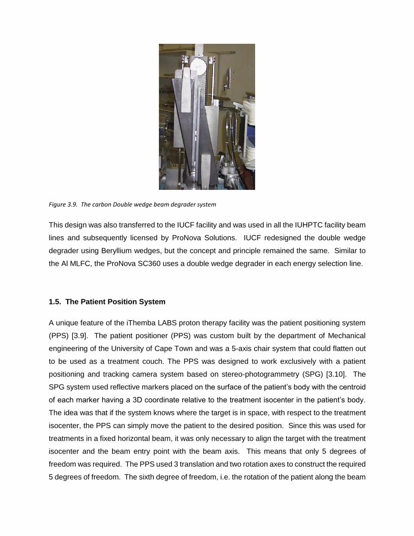
Figure 3.9. The carbon Double wedge beam degrader system

This design was also transferred to the IUCF facility and was used in all the IUHPTC facility beam

lines and subsequently licensed by ProNova Solutions. IUCF redesigned the double wedge

degrader using Beryllium wedges, but the concept and principle remained the same. Similar to

the Al MLFC, the ProNova SC360 uses a double wedge degrader in each energy selection line.

1.5. The Patient Position System

A unique feature of the iThemba LABS proton therapy facility was the patient positioning system

(PPS) [3.9]. The patient positioner (PPS) was custom built by the department of Mechanical

engineering of the University of Cape Town and was a 5-axis chair system that could flatten out

to be used as a treatment couch. The PPS was designed to work exclusively with a patient

positioning and tracking camera system based on stereo-photogrammetry (SPG) [3.10]. The

SPG system used reflective markers placed on the surface of the patient’s body with the centroid

of each marker having a 3D coordinate relative to the treatment isocenter in the patient’s body.

The idea was that if the system knows where the target is in space, with respect to the treatment

isocenter, the PPS can simply move the patient to the desired position. Since this was used for

treatments in a fixed horizontal beam, it was only necessary to align the target with the treatment

isocenter and the beam entry point with the beam axis. This means that only 5 degrees of

freedom was required. The PPS used 3 translation and two rotation axes to construct the required

5 degrees of freedom. The sixth degree of freedom, i.e. the rotation of the patient along the beam

axis, was corrected for by rotating the beam defining aperture to match the target outline in the

Beam’s eye view. Since the system initially used the shoot through and later, on the double

scattering beam delivery technique, rotating the aperture to obviate the need to align the patient

in three dimensions was acceptable and very efficient.

Figure 3.10: An illustration of the SPG patient positioning system.

This technique cannot be used in systems where the aperture cannot be rotated or where the

beam delivery coordinates cannot easily be rotated around the beam axis, e.g. pencil beam

scanning system. The principles of operation of the SPG patient positioning system are illustrated

in Figure 3.10. The PPS system worked incredibly well and was upgraded with many additional

features over the years. The system was able to monitor the patients position in real time at a

frequency of 4 Hz or more depending on the number of reflective targets that were monitored.

The system was also able to generate an interlock to interrupt the beam if the patient moved by

more than a set amount. A beams eye view x-ray was used to verify the patients position in the

beam for the first beam only

Figure 3.11: The design of the miniature ion chamber with physical dimensions in mm is shown in panel A. Panel B shows a few pictures of the miniature ion chamber with the water-tight Vespel seal cap removed in the top picture. Depth and transverse dose distributions obtained with the miniature ion chamber as compared to those measured with a diode, a diamond detector, a parallel plate ion chamber (Markus chamber) and a thimble chamber (Exradin T2) are shown in panels C and D respectively.

1.6. Dosimetry Aspects

A unique challenge in proton beam dose measurements is that the beam exhibits steep dose

gradients in both the transverse and longitudinal directions. The lateral penumbra in the shoot

through beams are extremely small while the proximal and distal dose gradients across the Bragg

peak are very steep. This basically means that one must use two types of detectors to measure

the lateral and longitudinal dose distributions which is very cumbersome. I developed a miniature

ionization chamber based on a very simple but unique technique that offered adequate resolution

to be used for transverse and longitudinal dose measurements [3.11]. The miniature ionization

chamber became the workhorse for dose measurements at many proton therapy centers such as

the Charité, Universitätsmedizin Berlin proton therapy facility, formerly known as the Hein Meitner

Institut for Nuclear Research, in Berlin, Germany and the IUHPTC in Indiana. The device was

also used to characterize the beam from the first prototype, the Tomo-Therapy machine that was

developed in Wisconsin. The dose distributions obtained with the miniature ion chamber as

compared to those measured with a diode, a diamond detector, and some thimble chambers are

shown in Figure 3.11.

2.0 PROTON THERAPY AT IUHPTC.

The Indiana University Health Proton Therapy center – abbreviated as IUHPTC, formerly known

as the Midwest Proton Radiotherapy Institute (MPRI), opened its doors for the first patient

treatments in Bloomington, Indiana, in February 2004. When IUHPTC treated its first patient, it

was only the third operating proton therapy facility in the United States that could treat large, deep

seated cancer targets with accelerated protons. When the IUHPTC facility was closed in

December 2014, it was the thirteenth proton therapy center in the USA. IUHPTC was located

adjacent to the Indiana University Cyclotron Facility (IUCF) [3.12] on the campus of Indiana

University and received the accelerated protons for patient treatments from IUCF’s open-sector

cyclotron. The IUHPTC project was initiated when the main National Science Foundation (NSF)

grant to IUCF ended and it was realized that the cyclotron provides adequate energy to be used

for cancer treatments. The IUHPTC facility had three operating proton treatment rooms. The

construction of the IUHPTC facility was structured in three main phases. Phase 1 dealt with

refurbishing the IUCF cyclotron and constructing the fixed horizontal beam treatment room

(FBTR) [3.13]. Phase 2 created the second treatment room, which was equipped with a 360-

degree rotating isocentric gantry supplied by Ion Beam Applications of Belgium. The final phase

involved constructing the third treatment room, which also contained an IBA 360-degree rotating

isocentric gantry.

This section focuses on the FBTR at IUHPTC, which was designed with two fixed beam lines,

one for large-field and deep-seated targets, called the fixed horizontal beam line (FHBL), and a

second one for shallow and small lesions in the orbit, also referred to as eye treatments or eye

beam line [3.14]. The latter was developed by IUCF in 1997 and was used to treat several Macula

degeneration cases but was never re-installed in the new fixed-beam treatment room.

2.1 Functional description of the fixed beam treatment room at IUHPTC.

The FBTR comprised of a beam delivery system (BDS) and a dose delivery system (DDS) that

includes the beam delivery nozzle, a patient positioner, and an x-ray system. A unique feature of

the IUHPTC system was that each proton treatment room at IUHPTC was equipped with its own

BDS. The function of the BDS is to extract the beam from the main trunk line, into which the

cyclotron delivers the accelerated protons at a fixed energy of 210 MeV but at variable intensities.

The appropriate energy required for a specific treatment was set uniquely by the BDS of each

room. This is illustrated in Figure 3.12 which shows the floor plan layout of the IUHPTC facility.

Figure 3.12: The floor plan of the IUHPTC (formerly known as MPRI). The following area are indicated on the drawing: A- 750KeV proton injector LINAC + 8 MeV injector cyclotron; B – 205 MeV Separated Sector Cyclotron, C – 205 MeV achromatic proton trunk line, D 65 – 205 MeV energy selection beam line, E Fixed Beam Treatment room (FBTR), F – 360 degree rotating gantry, G – Proton Clinical area and H – Radiation effects research Room.

This design renders the three proton treatment rooms virtually independent from each other and

from the cyclotron with respect to beam energy and setup. A method of active beam sharing

between the proton treatment rooms has been proposed but was never implemented [3.15]. The

ProNova system that received FDA approval in December 2016 and is in clinical operation at the

Provision Center for Proton Therapy in Nashville, TN USA, utilizes the exact same beam transport

and beam distribution system between treatment rooms. This is a perfect example where an

historic development at IUHPTC made it into a commercial application that will contribute

significantly to a more efficient beam utilization.

The BDS extracted the beam from the main trunk line in less than 3 msec. using a fast kicker

system. After extraction, the beam enters the energy selection system where it first passes

through an energy degrader consisting of a pair of Beryllium (Be) wedges that degrades the beam

to the desired energy for a specific beam to be delivered to the patient. As stated above, this

degrader design was modelled after the double wedge Carbon degrader that I designed and

implemented at the iThemba Labs facility. After leaving the degrader, the beam is bent 63

degrees by a dipole magnet to separate the lower energy protons, resulting from multiple

Coulomb scattering in the degrader, from the desired higher energy protons. A pair of horizontal

slits was used downstream of the 63 degree dipole magnet to cut away the unwanted low-energy

protons. An Al MLFC was used to analyze the beam energy characteristics during the so-called

“Prime” procedure that precedes any beam “Start” event. The BDS enforced the acceptable

criteria with respect to beam energy, energy spread, and intensity. After the “Prime” procedure

has succeeded, the beam was transported into the treatment room via a second 63 degree dipole

magnet. On entering the treatment room, the beam could be directed into either the FHBL or the

eye line using a +10degree switch magnet. Since the eye line was never re-installed, the switch

magnet was hard wired to bend the beam by +10 degrees and feed it into the FHBL nozzle. The

beam exits the beam line vacuum through an 80 micron thick Kapton vacuum window just

upstream of the switch magnet. The beam intensity was measured in real time using a secondary

emission monitor that was installed just upstream of the Kapton vacuum window. The first beam-

line element after the switch magnet was a multi-wire ionization chamber (MWIC), identical to the

one I designed and implemented at iThemba Labs [2.28], see section 1.3 above, that measured

the beam intensity profile in the horizontal and vertical planes. The signals from the MWIC were

used by the BDS to control the beam position at the entrance of the beam delivery nozzle.

2.2 The beam delivery nozzle

The beam delivery nozzle layout and the components for the fixed beam line were entirely

developed by me with the help of several mechanical and electrical engineers. The nozzle

employed passive scattering techniques to spread the beam to a maximum diameter of 20 cm at

the room isocenter. The room isocenter was 4 m from the center of the switching magnet. A two-

dimensional CAD rendering of the FHBL nozzle is shown in Figure 3.13.

A double scattering system, invented by Grusell [3.14] and designed by Gottschalk [3.17], for a

fixed energy of 210 MeV was used as the base design to passively spread the incident proton

beam to a finite size. A classic double scattering system uses two scatterers to spread the beam.

Typically, the first scatterer, of uniform thickness and high atomic number (Z), spreads the beam

isotropically in the forward direction, and a composite second scatterer scatters the beam more

strongly in the center than on the edges but presents the same energy loss to all the protons

passing through it [3.17]. One problem with double scattering systems is that the scattering power

of protons is dependent on energy, this means that a specific scattering configuration will only

work for one beam energy. To overcome this, most double scattering systems employed to date

used a multitude of first scatterers or combinations of different uniform-thickness materials to

constitute the first scatter for all possible beam energies. Another option was to degrade the beam

energy downstream of the double scattering system, but this leads to the production of unwanted

additional scatter and secondary neutrons close to the patient.

Figure 3.13: Diagram of IUHPTC TR1 fixed horizontal beam line Nozzle

I introduced a unique solution to this problem that simplifies the first scatterer problem. I

implemented a system that moves the first scatterer longitudinally along the beam axis as a

function of incident beam energy. This means that the distance between the first and second

scatterer is reduced as the energy decreases, which keeps the shape and size of the beam profile

on the second scatterer constant, regardless of the beam energy. However, due to space

limitations in the beam nozzle, it was not possible to move the first scatterer far enough

downstream to cover the entire incident energy range, i.e., energies from 208 to 70 MeV. This

was solved by using two composite first scatterers that exhibit different scattering powers but the

same energy loss to the incident beam.

The total energy loss in the beam delivery nozzle is a critical parameter that must be minimized

to attain the maximum range in water for the maximum incident beam energy. To minimize the

energy loss, the passive spreading system was optimized according to two maximum-field size

ranges with maximum diameters of 11.5 cm and 20 cm at the isocenter. This means that the two

field-size dependent configurations and the two beam range dependent options for each field size

option of the FHBL nozzle employ a total of four first scatterers and two second scatterers. All the

scatterers were mounted on two rotating carousels (one upstream and one downstream carousel)

that were manually set to the required combinations prior to a beam delivery event. The

thicknesses of the first and second scatterers for the mentioned field sizes are listed in Table 3.1,

and the designs of the second scatterers are shown in Figure 3.14.

Table 3.1: The thicknesses of the first and second scatterers for the mentioned field sizes.

Beam energies resulting in a range in water between 14 cm and 25.9 cm (the high-energy range)

required that the first upstream scatterer in each field size option is used while the second

upstream scatters were used for beam ranges less than 14 cm. For a specific beam range option

(high or low range), the position of the upstream scatterer was varied according to the incident

beam energy starting at the most upstream position, i.e., at the farthest distance from the

isocenter and second scatterer for the highest energy. The two upstream scatterers for each field

size group have the same energy loss but different scattering characteristics. This was achieved

by decreasing the Lead thickness of the low range upstream scatterer while adding a poly

carbonate layer to compensate for the range deficit because of the decreased lead thickness.

Although this might sound highly complicated, it solves a very complex problem by means of using

two field size dependent options in combination, with two range dependent options for each of

these options, i.e. a total of four combinations to achieve the goal of having a nozzle that can

provide field sizes up to 20 cm in diameter and ranges up to 25.9 cm.

Figure 3.14. The designs of the second scatterers showing the thickness of the Lucite and Lead as a function of the radial distance from the beam axis (left panel: small field scatterer, right panel: Large field scatterer)

Two anti-scatter collimators were used in the nozzle to remove the over-scattered protons from

the beam. The first collimator has a diameter of 5.5 cm and was located at a distance of 250 cm

from the isocenter, just downstream of the second scatterer carousel. The second anti-scatter

collimator has an inside diameter of 120 cm and was located 195 cm from the isocenter, just

upstream of the monitor ionization chambers.

The dose delivered to the patient was measured with two central-spot transmission parallel-plate

ionization chambers, while the beam symmetry was measured with two quadrant transmission

parallel-plate ionization chambers. All the ionization chambers were installed inside an ion

chamber assembly located at a distance of 185 from the room isocenter (see Figure 3.12), just

downstream of the second anti-scatter collimator. The ion chamber assembly also housed a

padded-array ion chamber that consisted of 30 small ionization chambers in each of the horizontal

and vertical planes. This array detector was installed to analyze the scanned beam characteristics

initially planned for the FHBL nozzle. It was foreseen that the FHBL nozzle would be upgraded in

the future to employ scan beam techniques identical to the gantry treatment rooms, using a

unique, combined-function scan magnet [3.16] to spread the beam magnetically in the x-y plane.

An exploded view of the ion chamber assembly as well as a detailed view of all the elements in

the assembly is shown in Figure 3.15

Figure 3.15. An exploded view of ion chamber assembly is shown in the left panel showing some of the ion chamber elements. The right panel shows the sequence of all the ion chamber elements that were installed in the ion chamber

housing.

Dose monitoring and termination was done with two specially designed dose monitor cards

(DMCs) referred to as DMC1 and DMC2. Each DMC provides its own enable and watchdog

signals to the beam control system (kicker enable system –KES). The DDS software pre-loads

the desired counts in terms of monitor units (MUs) into the counting registers of the DMCs and

sets the time limit on the DMCs. The software also drives a Digital to Analog Converter (DAC)

output to set the DMC calibration voltage (CVOLT). The electronic gain of each DMC counter was

adjusted by means of this CVOLT parameter. The reference CVOLT values were selected such

that 1 MU will result in 1 cGy of dose being delivered to the reference point for the reference beam

conditions. The reference CVOLT value for DMC2 was adjusted upward by 2% to make DMC2

2% less sensitive than DMC1. Each DMC drops it’s enabled signal to the kicker enable system

as soon as the accumulated counts reach the pre-loaded MUs. Since DMC2 was less sensitive

than DMC1, the dose termination was always generated by DMC1. Apart from preloading the

DMCs with the required set values, no software was involved in the dose measuring and

termination process. This was done entirely by the DMC hardware. The CVOLT values loaded

into the DMCs were corrected by a maximum of +2% to account for ambient temperature and

pressure changes. The set MU values on the DMC registers and the accumulated counts in the

DMC counters were read by the DDS control computer. These values were displayed on the DDS

graphic user interface (GUI) and the remote DDS console (using LED displays) in the external

control station manned by a radiotherapy technician (RTT).

A rotating modulator wheel was used to spread the pristine Bragg peak longitudinally to achieve

a spread-out Bragg Peak (SOBP). The modulator wheel was mounted on a retractable snout

assembly, discussed in the next paragraph, and rotates at a speed of 358 rpm. This means that

the longitudinal position of the modulator wheel varies according to the position of the retractable

snout, which is a function of the depth of the isocenter in the patient as well as the air gap between

the patient’s skin and the final patient aperture. A library of 16 modulator wheels was used to

provide the required clinically relevant SOBPs.

The last nozzle component before the beam enters the patient was the snout mechanism that

holds the final patient-specific aperture and compensator. Two different snouts exist for the

FHBL. The small-field snout could accommodate apertures with a maximum inside diameter of

10.9 cm (outside diameter of 11.5cm) and the medium-field snout could accommodate apertures

with a maximum inside diameter of 19 cm. The snouts attached to the snout translation

mechanism via a quick-release mechanism and the robotic patient positioner was used to

exchange the snouts. The final patient apertures were milled from solid brass, and the

compensators were made from acrylic (Lucite®) using computer numerical control milling

machines. The correct combination of the scatters, which depends on the beam range and

mounted snout, was monitored and verified by the DDS.

2.3 Beam Control

Although the DDS could not do any beam steering, it displayed the beam position and symmetry

parameters on the DDS GUI in the external RTT control station. The physicist on duty could adjust

the steering magnets controlled by the BDS to adjust the beam position and symmetry in the DDS

nozzle. The BDS displayed the beam position at the entrance to the nozzle on a BDS GUI in the

external RTT control station. The DDS measured the beam position in the nozzle by using data

from the two linear arrays of pad ionization chambers mentioned above. These ionization

chambers were arranged in horizontal and vertical arrays. The DDS software calculated and

displayed the skewness and kurtosis parameters of the beam in the vertical and horizontal

directions based on the readings from the pad ionization chambers. Using these parameters and

the actual display of the pad readings, the physicist could clearly distinguish if the beam was

properly positioned in the nozzle. The DDS measured the beam symmetry in the nozzle by means

of two quadrant ionization chambers. The ionization currents from the two upper and the two lower

quadrants of the first quadrant chamber were summed to determine the beam intensity in the

upper and lower halves of the beam. Similarly, the left and right-hand beam intensities were

obtained by summing the left and right quadrants of the second quadrant ionization chamber. The

up/down (U/D) and left/right (L/R) symmetries were displayed as the ratios of the summed

quadrant readings. A software calibration factor was applied to ensure that both ratios were equal

to unity when the beam was symmetrical in the nozzle. The DDS software terminates the dose

delivery as soon as these ratios exceed the symmetry limits of +2.5%, i.e., 0.975 < U/D or L/R <

1.025.

2.4 Range in water

The proton beam energy was characterized in terms of range in water rather than MeV since it is

an easily measurable quantity. The proton beam range in water was measured with a parallel

plate ionization chamber (Markus; PTW-Germany) since obtaining the depth of measurement for

this chamber using a high precision caliper was quite easy. This allowed for an accurate

determination of the beam range in water which is defined at the distal 90% dose point on the

Bragg curve when the maximum dose point on the peak is normalized to 100%. A 3D scanning

water phantom system (Wellhöfer Dosimetry; Blue Phantom) was used to move the Markus

chamber along the beam axis. A set of pristine Bragg peaks measured for different incident

energies with the parallel–plate Markus chamber is shown in Figure 3.16. The beam energy was

modified by the BDS, as described above. The maximum range in water of 25.9 cm was attained

for the small field geometry where the thinnest scatterers were required to produce a flat beam

(see Table 3).

Figure 3.16. Measured pristine Bragg peaks for different incident beam energies.

The full width at half maximum (FWHM) of the maximum energy beam was 23 mm, and the

distance between the distal 90% and 10% distal dose points was 5.9 mm (80 % – 20 % = 4 mm).

For the lowest incident energy, measured (R50 = 3.86 cm), these numbers reduce to a FWHM of

11.1 mm and a distal 90% to 10% falloff of 4 mm (80% – 20% = 2.3 mm).

2.5 Beam Flatness and Symmetry

The proton beam is spread laterally by means of the unique passive beam-spreading technique

described above. The left panel of Figure 3.17. shows the optimized positions of the upstream

scatterers as a function of incident beam energy (R50 range in water). The same positions were

used for the upstream scatterers for both field size options. As a result of modifying the position

of the first scatterer, the source-to-axis distance (SAD) of the FHBL is not constant, but rather a

function of the incident beam energy. The SAD is defined as the distance between the effective

source position and the room isocenter. We used the XIO treatment planning system developed

by Computerized Medical Systems INC (CMS), St. Louis USA (CMS was later acquired by

ELEKTA INC, Stockholm, Sweden). The XIO system could not accommodate a varying SAD but

since the proton dose calculation engine that was employed by XIO at that stage was not able to

calculate the beam output factor, the impact on a varying SAD on the calculated penumbra was

not clinically significant. The output factor for each beam was measured prior to starting a

treatment plan. As illustrated in figure 3.17, the SAD varied between 300 and 335 cm for the

clinical beam energies used i.e. beam ranges in water between 6 and 28 cm. This means that

the inverse square law alone contributed as much as 24.7 % to the change in the output factor

over the clinical energy range. The variation of the SAD as a function of beam range in water is

shown in the right panel of Figure 3.17.

Figure 3.17. Optimized positions of the first scatterer as a function of BDS requested range are shown in the left panel. The measured effective source positions as a function of the BDS requested range in water are shown in the right panel. This can be ascribed to the fact that the position of the first scatterer changes as a function of the BDS requested range in water and hence the changes in the effective source position. The solid lines are simply drawn to guide the eye

The beam flatness and symmetry were measured in a three-dimensional water phantom using a

miniature ionization chamber that was developed at iThemba LABs as discussed earlier in this

chapter [3.9]. The beam flatness is defined as the dose variation over the dose reference volume.

As shown in Figure 3.18, the measured data was within the ±2.5% flatness specification. The

beam monitoring system allowed the user to maintain a symmetrical beam.

2.6 Penumbra

The beam penumbra is defined as the lateral distance between the 80% and 20% dose points.

Beam penumbra data for several beam energies at different depths for beams with diameters of

3 and 10 cm diameter beams are shown in Figure 3.18. The penumbra data, as a function of the

air gap between the final patient aperture and the surface of the three-dimensional water tank, is

shown in Figure 3.10. The penumbra data were measured with the miniature ionization chamber

that I developed at iThemba LABS [3.11] which had an inner diameter of 1.9 mm to achieve a

sufficiently high measurement resolution to quantify the beam penumbra.

Figure 3.18. Measured lateral profiles for different beam energies (R50 – 50 % Range in water) at different depths. The dashed lines indicate the + 2.5 % flatness specification.

Figure 3.19: The 80–20% penumbra data measured in pristine beams with R50 ranges of 26.2 and 16 cm for 30 and 100 mm diameter apertures (Left Panel). Measured 80–20 % penumbra data in pristine and SOBP beams for different air gaps for the highest energy beam (206.5 MeV; R50 = 26.2 cm) are shown in the right panel.

2.7 Beam Modulation

The proton beam energy is modulated with downstream Lucite® propellers [3.4]. I designed a

library of propellers that modulated the proton energy to produce the required SOBPs. The

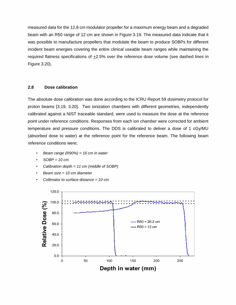
measured data for the 12.8 cm modulator propeller for a maximum energy beam and a degraded

beam with an R50 range of 12 cm are shown in Figure 3.19. The measured data indicate that it

was possible to manufacture propellers that modulate the beam to produce SOBPs for different

incident beam energies covering the entire clinical useable beam ranges while maintaining the

required flatness specifications of +2.5% over the reference dose volume (see dashed lines in

Figure 3.20).

2.8 Dose calibration

The absolute dose calibration was done according to the ICRU Report 59 dosimetry protocol for

proton beams [3.19, 3.20]. Two ionization chambers with different geometries, independently

calibrated against a NIST traceable standard, were used to measure the dose at the reference

point under reference conditions. Responses from each ion chamber were corrected for ambient

temperature and pressure conditions. The DDS is calibrated to deliver a dose of 1 cGy/MU

(absorbed dose to water) at the reference point for the reference beam. The following beam

reference conditions were;

• Beam range (R90%) = 16 cm in water

• SOBP = 10 cm

• Calibration depth = 11 cm (middle of SOBP)

• Beam size = 10 cm diameter

• Collimator to surface distance = 10 cm

Figure 3.20: Measured Depth Dose curves for the 12.8 cm SOBP propeller for a maximum energy beam and a R50 = 12 cm beam. The dashed lines indicate the + 2.5 % dose uniformity specification.

2.9 Robotic PPS

IUHPTC used robotic patient positioners in all the proton treatment rooms [3.21]. The positioners

were designed and developed at IUCF under my supervision and were based on work that I

started at the iThemba LABS. The patient’s position, with respect to the treatment room isocenter

and specific beam orientation, was verified with the x-ray system. The x-ray system was

comprised of three orthogonal x-ray sources installed at fixed locations in the treatment room and

one digital radiographic panel. This panel was moved into one of three positions, according to the

selected xray source, using a commercially available industrial robot arm with a maximum payload

of 20 kg (Motoman Model UP20) [3.21].

The design goal for the robotic PPS was to use a commercial robotic arm and implement it as a

patient positioner without modifying the robot. The approach was similar to the concept first

proposed by Mazal from CPO where a patient positioner based on a 300 Kg payload commercial

FANUC robot was developed [3.22, 3.23]. The main reasons for this approach were to save costs

and to capitalize on the extreme reliability of these devices. The project at iThemba labs never

came to fruition, but the robotic PPS developed at IUHPTC was used to position patients for

therapy, from the very first patient in 2004 to the last, when the facility shut down in 2014. The

design approach and functionality of the system is described in detail by Allgower et al. [3.24]. A

photograph of the IUHPTC system is shown in the right panel of Figure 3.21. The PPS was based

on a commercially available Motoman UP200 robotic arm designed for a 200 kg payload. These

devices are capable of extreme accelerations and high speeds.

Figure 3.21. The IUHPTC robotic patient positioner. It was based on the concept (left panel) proposed by Mazal et. al. from CPO in Paris.

As described by Allgower et al. [3.24], accelerometers and inclinometers were attached to the

PPS to measure the acceleration and inclination of the treatment bed continuously, to safeguard

the system. A unique feature of the IUHPTC and CPO robotic positioners was that these devices

were truly used as robots. In addition to using them as patient positioners, they were also used

to position heavy physics equipment such as the big 3D water phantom and to exchange the

beam defining snouts in all the treatment rooms where these devices were implemented. As can

be seen in Figure 3.21, the single arm design of the UP200 machine simplified the design of the

rotating floor over the robot pit. It is interesting to note that the only downtime suffered from this

system was related to the rotating floor around the PPS. I also designed a treatment chair that

could attach to the robotic PPS system to allow for intracranial treatments in the seated position.

This work was a continuation of work that I started in South Africa at the iThemba Labs facility.

Several patients were treated in the seated position until the first one of two 360 degree isocentric

gantries was commissioned for clinical use in 2006. A photograph of the chair attached to the

PPS is shown in Figure 3.22. The docking trolley that transported the chair could be docked in a

very reproducible position in the treatment room. A robot program was run on the PPS to pick up

the chair. The docking trolley is also visible in Figure 3.22.

Figure 3.22. The treatment chair for intra cranial treatments in the fixed beam room. The transport cart secured in the docking position is also shown.

A unique feature that I modelled after the system used at the Harvard Cyclotron facility for seated

treatments, was that every patient had a custom-made wooden backrest. The respective

immobilization devices were permanently affixed to the wooden backrest and pieces of the

backrest that might interfere with the beam could simply be cut away with a hacksaw. The wooden

backrest is also visible in Figure 3.22.

3.0 DEVELOPMENTS AT PROCURE TREATMENT CENTERS.

ProCure Treatment centers was founded to own and operate a network of proton therapy centers

across the USA. Cost reduction and reliability were two major considerations to make the

business plan work. Two major initiatives that ProCure treatment centers embarked upon was

the development of the dual fixed beam treatment room, referred to as the inclined beam

treatment room [3.25], as well as a unique robotic positioner. Since ProCure was anticipating a

major expansion of proton therapy in the United States and internationally, I proposed that we

develop a training and development center (TDC) in Bloomington, Indiana, USA. The TDC was

a proton therapy training facility, fully equipped with all the proton therapy software, i.e. treatment

planning (XIO) and oncology information system (Mosaiq OIS), a CT scanner (GE) and one 360

degree gantry, and one inclined beam treatment room simulator. The treatment room simulators

were built by Forte Automation and all the unique systems employed by the ProCure treatment

centers were first prototyped and installed at the TDC and subsequently used for staff training.

3.1 The Inclined beamline treatment room

The inclined beam treatment room was entirely based off a paper that I published in 1998 while

still at iThemba LABS. The title of the paper was, “The Non-orthogonal Fixed Beam Arrangement

for the Second Proton Therapy Facility at the National Accelerator Centre” [3.25]. ProCure

treatment centers developed four proton therapy facilities together with IBA, with two of the

inclined beam treatment rooms at each facility, for a total of eight inclined beam treatment rooms.

The 1998 paper stated three design prerequisites to make the inclined beam concept work. These

were that the system must:

(1) be equipped with Pencil Beam scanning nozzles,

(2) allow for Volumetric imaging at isocenter and

(3) have a sophisticated patient positioner that can position the patient in a seated position at

isocenter.

None of these prerequisites were initially achieved when the first patients were treated in the first

inclined beam at the Oklahoma City proton therapy facility. A Head and Neck chair was added to

all the facilities by 2012, but it was only in 2019 that one of the inclined beam systems at the

Chicago proton therapy facility was retrofitted with PBS. None of the inclined beam systems in

operation have been equipped with volumetric imaging at isocenter. The enormous reduction in

the size of the inclined beam system versus the IBA 360 degree isocentric gantry is illustrated in

Figure 3.23. The insert in the left panel shows the inclined beam system approximately scaled to

the gantry system shown in the left panel. The right panel of Figure 3.23 shows the inside of one

of the inclined beam treatment rooms at the Chicago proton therapy facility.

Figure 3.23. The reduction in the size of the inclined beam system versus the IBA 360 degree isocentric gantry. The insert in the left panel shows the inclined beam system approximately scaled to the gantry system also shown in the left panel. The right panel shows the inside of one of the inclined beam treatment rooms at the Chicago proton therapy facility

3.2 The Third-generation Robotic Patient Positioner

The valuable experiences gained from developing the Themba LABS and IUHPTC robotic patient

positioners were realized when I developed the third-generation robotic patient positioner together

with Forte Automation after joining ProCure Treatment centers. The Forte / ProCure Robotic PPS

was a great success and is generally referred to as the third-generation robotic patient positioner.

The system was installed in more than 70 proton therapy treatment rooms as the design was

adopted by most of the proton vendors. The design trial of the Forte / Procure PPS is illustrated

in Figure 3.24. We started with a standard, commercially available, articulated 6 axis Kuka robot

arm, as shown in the left panel of Figure 3.24, which was similar to the concept employed by the

IUHPTC positioners and the system developed by Siemens [3.26]. During many simulations, I

found that mounting the robot vertically resulted in too many mechanical interferences with the

tabletop and I introduced the concept of mounting the upper arm horizontally as shown in the

middle panel of Figure 3.24. This configuration robot is referred to a SCARA type robot which

employs one linear axis (the vertical up and down motion axis) and 5 rotational axes. Toby

Henderson – the CEO of Forte Automation – then decided to make a custom arm and only re-use

the wrist section of the commercial Kuka robot. The system was also equipped with gear

reduction gearboxes to slow the robot down for safety purposes.

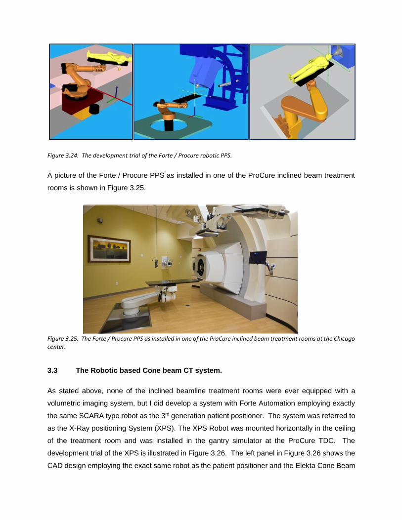
Figure 3.24. The development trial of the Forte / Procure robotic PPS.

A picture of the Forte / Procure PPS as installed in one of the ProCure inclined beam treatment

rooms is shown in Figure 3.25.

Figure 3.25. The Forte / Procure PPS as installed in one of the ProCure inclined beam treatment rooms at the Chicago center.

3.3 The Robotic based Cone beam CT system.

As stated above, none of the inclined beamline treatment rooms were ever equipped with a

volumetric imaging system, but I did develop a system with Forte Automation employing exactly

the same SCARA type robot as the 3rd generation patient positioner. The system was referred to

as the X-Ray positioning System (XPS). The XPS Robot was mounted horizontally in the ceiling

of the treatment room and was installed in the gantry simulator at the ProCure TDC. The

development trial of the XPS is illustrated in Figure 3.26. The left panel in Figure 3.26 shows the

CAD design employing the exact same robot as the patient positioner and the Elekta Cone Beam

CT (CBCT) system mounted on the robot. The middle panel shows the system installed at the

TDC and the first CBCT images of a head phantom are shown in the right panel. The system

was, however, not deemed financially viable and the development was abandoned in 2011. In

retrospect, this was a major mistake and should have been further pursued.

Figure 3.26. The ProCure XPS development trial. The left panel shows the CAD design of the system while the middle panel shows the XPS as was installed at the TDC. The right panel shows coronal, sagittal and axial CBCT images of a head phantom obtained with the system.

3.4 A treatment chair for seated treatments.

It was obvious that to increase the utilization of the ProCure inclined beam treatment rooms we

needed to be able to treat the patients in a seated position. I again developed a treatment chair

that could be picked up by the robotic positioner using the quick coupler mechanism that was

installed to the end effector of the PPS robot. Similar to the system I developed at IUHPTC, the

PPS robot can decouple from the tabletop and couple to the chair. This was all automated using

the PPS robot in a true robotic fashion. The development trail of the ProCure treatment chair is

illustrated in Figure 3.27. The left panel shows a CAD drawing of the chair coupled to the end

effector of the PPS overlaid on the treatment bed. The middle panel in Figure 3.27 shows the

prototype system during the PPS chair coupling process. The transport cart docked into a

reproducible position in the room can also be seen. The right panel in Figure 3.27 shows the first

patient treated in the chair at the Oklahoma proton therapy facility.

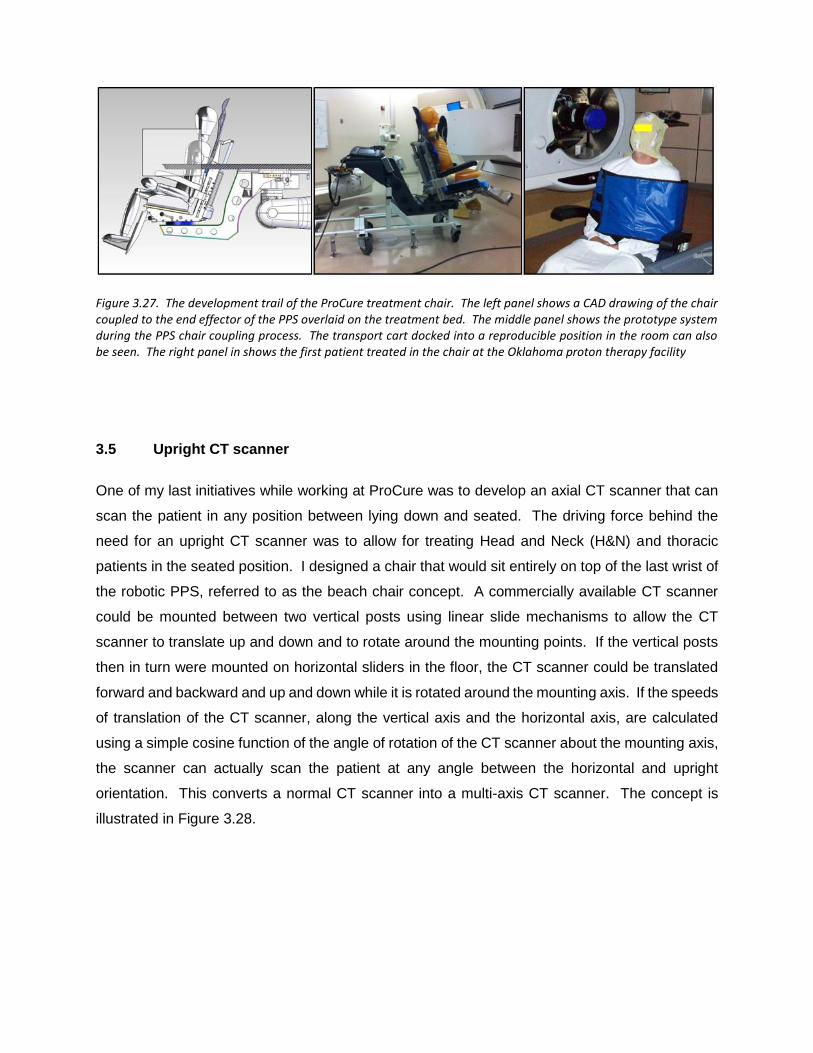
Figure 3.27. The development trail of the ProCure treatment chair. The left panel shows a CAD drawing of the chair coupled to the end effector of the PPS overlaid on the treatment bed. The middle panel shows the prototype system during the PPS chair coupling process. The transport cart docked into a reproducible position in the room can also be seen. The right panel in shows the first patient treated in the chair at the Oklahoma proton therapy facility

3.5 Upright CT scanner

One of my last initiatives while working at ProCure was to develop an axial CT scanner that can

scan the patient in any position between lying down and seated. The driving force behind the

need for an upright CT scanner was to allow for treating Head and Neck (H&N) and thoracic

patients in the seated position. I designed a chair that would sit entirely on top of the last wrist of

the robotic PPS, referred to as the beach chair concept. A commercially available CT scanner

could be mounted between two vertical posts using linear slide mechanisms to allow the CT

scanner to translate up and down and to rotate around the mounting points. If the vertical posts

then in turn were mounted on horizontal sliders in the floor, the CT scanner could be translated

forward and backward and up and down while it is rotated around the mounting axis. If the speeds

of translation of the CT scanner, along the vertical axis and the horizontal axis, are calculated

using a simple cosine function of the angle of rotation of the CT scanner about the mounting axis,

the scanner can actually scan the patient at any angle between the horizontal and upright

orientation. This converts a normal CT scanner into a multi-axis CT scanner. The concept is

illustrated in Figure 3.28.

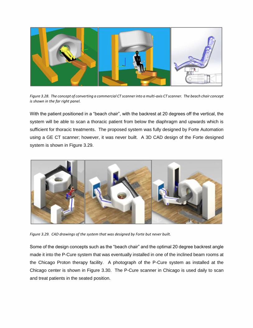
Figure 3.28. The concept of converting a commercial CT scanner into a multi-axis CT scanner. The beach chair concept is shown in the far right panel.

With the patient positioned in a “beach chair”, with the backrest at 20 degrees off the vertical, the

system will be able to scan a thoracic patient from below the diaphragm and upwards which is

sufficient for thoracic treatments. The proposed system was fully designed by Forte Automation

using a GE CT scanner; however, it was never built. A 3D CAD design of the Forte designed

system is shown in Figure 3.29.

Figure 3.29. CAD drawings of the system that was designed by Forte but never built.

Some of the design concepts such as the “beach chair” and the optimal 20 degree backrest angle

made it into the P-Cure system that was eventually installed in one of the inclined beam rooms at

the Chicago Proton therapy facility. A photograph of the P-Cure system as installed at the

Chicago center is shown in Figure 3.30. The P-Cure scanner in Chicago is used daily to scan

and treat patients in the seated position.

Figure 3.30. A photograph of the P-Cure upright CT scanner installed in the Chicago Proton Therapy facility.

4. SUMMARY

My initial experiences and exposure to the fundamental aspects of proton therapy technologies

and physics at the iThemba LABS prepared me to embark on many more developments and

innovations over the next years at the IHPTC and at ProCure. The ever-developing field of proton

therapy and the fact that the proton therapy technologies are expensive, continues to provide

opportunities to innovate in the pursuit of reducing costs through improved technologies and

improved efficiencies. The initiative that I led at iThemba LABS to do away with rotating gantries

and rather treat the patient in a seated or upright position is now finally gaining traction world-

wide. Several companies are now developing technologies that I believe will allow for substantial

cost reduction of proton therapy, while also improving the treatment delivery efficiencies. This

will undoubtedly lead to the improvement of beam delivery since more people will get involved in

proton therapy and more money will be available to develop and improve the technologies,

especially in the area of real time imaging. I discuss these aspects in more detail in chapter 5 of

this thesis.

CHAPTER 4:

THE CLINICAL REALIZATION OF PENCIL BEAM SCANNING AND THE

ENORMOUS IMPACT ON THE USABILITY OF PROTONS IN CLINICAL

PRACTICE.

4.1. OVERVIEW:

This chapter will address the current uses of Pencil beam scanning (PBS) in state-of-the-art

clinical proton therapy facilities and the enormous benefits that the PBS techniques brought to

the field of proton therapy. The chapter is based on some sections from an invited paper that I

authored together with the clinical medical physics team at the Provision Center for Proton

Therapy in Knoxville (PCPTK) in 2016. The paper is titled, “A Review of Proton Radiation Therapy

and the Path to Widespread Clinical Adoption” and was published the Medical Physics

International Journal in 2016 [4.1]. The header info for the published paper is shown in figure 4.1.

I developed the framework for this paper and invited the entire medical physics team to participate.

I wrote the bulk of the paper, but the team participated actively in the process. Dr. Fagundes was

awarded the senior author status for this paper since he was the Medical Director of the facility at

that time.

In this chapter, I discuss the advances and benefits that pencil beam scanning (PBS) brought to

proton therapy. Clinical examples for the most appropriate targets are discussed and arguments

towards proton certainties in dose deliveries versus the traditional uncertainties are developed.

With PBS, proton therapy is no longer limited to smaller and contiguous targets, but can bring the

largest clinical benefit to larger, distributed, and often more advanced cancers that can still be

treated radically (with a view to achieving a cure). These include cancers where the lymph nodes

need to be treated prophylactically or curatively, e.g. breast, Head and Neck (H&N), and high-

risk prostate cancers.

Figure 4.1: The header for the Invited paper published in the Medical Physics International Journal

4.2. INTRODUCTION

After many years of development, proton therapy is finally reaching the point of mass adoption in

clinical practice world-wide. This is mainly due to three contributing factors: advances in

accelerating technology, advances in beam delivery techniques, and excellent clinical results.

Firstly, technological developments have made proton therapy systems commercially available

and allowed these systems to become more compact and less expensive [2.1]. Secondly, the

clinical realization of pencil beam scanning (PBS) has allowed proton therapy to be more in-line

with modern day state-of-the-art intensity modulated x-ray radiation therapy (IMRT) treatments.

Thirdly, the widespread adoption of proton therapy that is now happening is fully justified on the

basis of early clinical and technical research and developments.

PBS is the generic name for delivering radiation dose to a target using individually controlled

pencil beams of accelerated protons to cover a target in 3 dimensions. The first proton patients

were treated with PBS at the Paul Scherrer Institute in Switzerland in 1996, but it took the industry

many years to commercialize the system and make it available at more facilities [2.31, 2.32].

Today, PBS is in routine clinical use in a majority of proton therapy facilities across the globe.

The increased flexibility in dose shaping has enabled improved dose conformation, especially to

large and non-contiguous targets, and truly revolutionized proton therapy in the last few years.

The general utilization of proton therapy has been expanded to almost all sites in the body and,

with robust optimization, which is a practical solution only with PBS, the traditional problems with

range uncertainties have been addressed to a greater extent [2.39]. Using intelligent optimization

strategies and computer algorithms, treatment plans are now optimized with the perceived

uncertainties in mind, rendering the delivered plans robust against changes and uncertainties in

the entire treatment process [4.1, 4.2]. We can now talk about the certainties, rather than the

uncertainties, in PBS proton beam delivery, which provides physicians with vastly improved

confidence in the delivered target dose. The largest paradigm shift caused by PBS is that we are

now faced with the question of which targets, from a treatment planning perspective, will not

benefit from proton therapy, rather than the traditionally inverse question.

4.3. TECHNOLOGY DEVELOPMENTS – PENCIL BEAM SCANNING

Recent advances in the proton therapy industry are changing the way the technology is used.

New techniques in beam delivery, treatment planning, and image guidance are improving the

quality of treatments for current treatment sites and opening the door for sites not previously

treated with protons. As stated before, the most significant advancement in recent years has

been the widespread adoption of PBS delivery techniques. Whereas early proton treatment

systems relied on spreading the beam and then shaping it through the use of patient specific

apertures and compensators, PBS actively controls a thin pencil beam, steering it to deliver dose

in discrete “spots”.

Early proton beam delivery methods used double scattering (DS) or “uniform” magnetic scanning

(US) to spread the beam over a larger area than necessary and required apertures and

compensators to shape the beam laterally and distally. The only beam parameters that could be

adjusted were the range and modulation, or width, of the SOBP. Effectively, one could choose

how deep to deliver the beam, conform the distal end to the target with a compensator, and decide

how far to pull back the high dose region [2.26, 2.27]. By necessity, the shape of the proximal

high-dose region would mimic the shape of the distal end, since the dose could only be uniformly

modulated, or pulled back. The physics thus give rise to unintended proximal high dose areas

outside the target for each individual beam. This effect is mitigated through the use of multiple

beams, similar to 3D photon-based techniques. Likewise, there is no freedom to adjust the width

of the beam at different depths since the aperture, which cannot change for a given beam,

provides all lateral shaping. These previous delivery techniques benefited from the physics of

protons, which includes reduced entrance dose and no exit dose, but were severely limited by

lack of freedom in shaping the dose distribution within the patient. Figure

4.2 illustrates the beam design for traditional proton therapy.

Figure 4.2. An illustration of traditional proton therapy using DS or US, where the beam is shaped with an aperture and the distal dose is conformed to the target with a compensator that corrects for the distal shape of the target (1), the oblique incidence of the beam (2) and inhomogeneities (3) in the beam path.

The advent of pencil beam scanning delivery techniques has overcome these disadvantages. In

PBS, the beam is actively steered to deliver dose in discrete “spots” at given depths and lateral

offsets. This is illustrated in figure 4.3. PBS therefore gives the treatment planner full control over

how and where dose is deposited from each beam. Choosing the spot locations allows for

changing the beam width with each energy layer. Using this technique, the high dose can conform

to both the distal and proximal ends of the target or create a concave shape on the lateral edge

of the beam. Compared to 3D proton therapy, PBS allows for improved proximal sparing and

does not require apertures and compensators.

Figure 4.3. An illustration of the PBS technique. PBS is uses individually controlled small pencil beams of accelerated protons to cover a target in 3 dimensions. The individual pencil beams are scanned off-axis with a fast scanning electromagnet. The beam is stationary at a spot until the desired dose for each spot is delivered.

The only side effect that PBS cannot avoid is that each spot must still deposit its entrance dose.

An advantageous clinical application of the proximal sparing of PBS is in the treatment of breast

cancer discussed in section VI. A simple single beam comparison between a DS/US and a PBS

beam for a target in the brain is shown in figure 4.4. The freedom and flexibility provided by PBS

opens the door to other advanced planning techniques. In earlier delivery methods, each beam

could only deliver a nominally uniform dose, with unintended hot and cold spots resulting from

scattering in the patient’s anatomy or compensator. With PBS, it is possible, and often sufficient,

to mimic this technique, with each field giving a uniform dose to the target; however, this is no

longer a requirement. If desired, each beam can be optimized to conform the desired isodose to

the target, based on that particular beam’s eye view. For example, if a clinical target volume

(CTV) wraps around an organ-at-risk (OAR), a right lateral beam may deliver more dose to the

near (right hand) side of the CTV, and less dose to the far side, which would require passing

through the OAR. The severity of this biasing can be adjusted to any degree the planner prefers.

Figure 4.4. The difference in dose between a single proton beam delivered with DS/US and with PBS. The bottom right panel shows the unnecessary dose delivered outside the target area with US/DS.

In addition to new beam delivery technologies, proton treatment planning techniques are

progressing. Monte Carlo based dose calculation will soon become mainstream, allowing more

accurate dose calculations for difficult geometries and providing additional information to the

treatment planner [2.25, 4.38]. Pencil beam dose calculation algorithms for protons have always

struggled to model upstream scatter, such as through a thick compensator. With PBS, the

problem becomes the range shifter. For most proton therapy systems, there exists a lower energy

limit – typically 75 MeV, or approximately 4 cm range in water. Outputting energies lower than

this limit would require too much degrader material in the beam path, which would reduce the

dose rate and increase the spot size. To mitigate this issue, a range shifter is utilized, as needed.

A range shifter is a piece of acrylic placed in the beam, near the patient, that can further degrade

the beam to energies low enough for shallow targets, such as breast treatments. The range

shifter is positioned outside of the vacuum in the delivery system, so the protons will scatter in air.

The air gap is defined as the distance between the range shifter and the patient, and a shorter air

gap will scatter the beam less. For large air gaps with a thick range shifter, the algorithm may

overestimate the shallow dose. Monte Carlo calculations greatly improve the accuracy of the

dose calculation with upstream scatterers, as well as in the presence of heterogeneities such as

air pockets, lung, and metal implants [2.40, 2.41].

One widespread unknown in proton therapy is the relative biological effectiveness (RBE) of

protons relative to photons. It has become standard to use a factor of 1.1 [4.3], so that everyone

will be “equally wrong”. However, we know that RBE is tied to the Linear Energy Transfer (LET)

of the protons at any point in their slowing down process, and the LET varies with energy. It is

this variation of LET with energy that produces the Bragg peak. With Monte Carlo dose

calculations, one can view LET-weighted dose distributions to evaluate what areas might be at

risk of elevated biological doses and minimize this effect, or at least ensure that it does not occur

in sensitive critical structures. Once LET-to-RBE relationships are better established, biologically

optimized plans should become possible.

4.4. ADVANCES AND EFFICIENCIES IN PBS TREATMENT PLANNING

Traditional treatment planning in proton therapy requires the use of apertures and compensators.

Apertures are typically made of brass and are used to limit the field size for each beam.

Compensators are made of Lucite or wax and provide distal range conformation for each beam.

This range conformation accounts for tissue compensation, as well as distal organ-at-risk (OAR)

sparing. Treatment planning using apertures and compensators is very similar to 3D conventional

photon planning. A target is contoured on several slices in the CT scan and beams are chosen

to reduce uncertainties and spare normal tissues. Typically, 1-3 beams are sufficient for most

proton targets, regardless of the proton modality. Beam angle uncertainties can include

immobilization device uncertainty, patient inhomogeneity uncertainty, and target motion

uncertainty. These uncertainties must be considered, even in more modern PBS treatment

planning. For each beam in a DS or US plan, an aperture is developed by adding a lateral margin

around the target. If aggressive sparing is required from a certain beam angle, the aperture can

exclude a portion of the target. Margins must also be added proximally and distally to the target,

essentially widening the SOBP. This accounts for uncertainties both in the HU-to-stopping-power

conversion as well as uncertainties in the compensator design [2.39, 4.4]. A beam-specific

compensator is developed to account for tissue compensation in order to conform the dose to the

distal end of the target and for distal OAR sparing. Robust evaluation of a plan is performed,

determining if coverage is sufficient if the patient shifts or if the HU-to-stopping power conversion

is slightly off. This includes shifting the isocenter in 6 directions and evaluating a denser and less

dense CT. This concept of robust evaluation obviates the need for a Planning Target Volume

(PTV). In photon therapy, a PTV is typically a uniform margin around the Clinical Target Volume

(CTV) that accounts for patient setup variations [4.16]. In proton therapy, a beam specific PTV,

which includes lateral, distal, and proximal margins, is required. However, since each beam will

be treated with different energies, the distal and proximal margins will vary per beam, hence a

beam specific PTV. The catch 22 situation is that you don’t know the beam angles until you make

the plan, but you need the PTV before you start the plan. This problem is now mitigated with PBS

robust optimization, as I will discuss later.

After the plan is approved, the design for each aperture and compensator can be manufactured

on or off site. Quality Assurance (QA) should then be performed on each aperture and

compensator, prior to treatment. For each patient, there is typically one aperture and

compensator pair per beam. If a cone down or an adaptive plan is necessary, new apertures and

compensators may need to be designed and manufactured. With the development of PBS, the

need for apertures and compensators practically vanished. PBS offers the ability to place spots

precisely within the target for each energy layer, negating the need for an aperture to define the

field size (see figure 4.4 above). Additionally, since each layer can be optimized, there is no need

for a compensator. This leads to a very different type of treatment planning for proton therapy

that is very similar to IMRT treatment planning, i.e. an inverse optimization technique, referred to

as inverse planning. The treatment planner instructs the optimizer what targets to treat and what

OARs to spare and the optimizer will choose the number of layers, location, and intensity of each

spot per layer. The need for stable and well-characterized immobilization as well as the need for

well-thought-out beam angles has remained very similar to 3D proton planning.

One of the most advantageous and publicized treatment sites for proton therapy is Cranial Spinal

Irradiation (CSI), particularly in pediatrics [4.6, 4.7]. One of the challenges of a CSI treatment is

accounting for the necessary match line within the treatment field. CSI treatments require match

lines due to the large field sizes when treating the brain and the entire spine. Another treatment

site requiring match lines is head and neck treatments, due to the need for ideal beam angles to

avoid uncertainties and healthy tissues. In 3D proton planning, as in 3D photon planning, match

lines require the use of feathering. With the sharp beam edge defined by an aperture, a very

precise gap must be left between the beams, causing significant cold or hot spots in the junction

if the gap is not reproduced accurately during treatment. The usual mitigation for this effect is to

shift the beam junction, a tedious process requiring at least a second set of fields (and apertures).

Another downside is that this tactic leads to extreme sensitivity in the shifting of the patient from

one isocenter to the next. Shifting too far could greatly increase the cold spot in the junction and

shifting too little could create a severe hotspot. With the use of PBS treatment planning, a gradient

can be developed between abutting fields that can raise or lower the dose for each field [4.8] over

a larger distance. This gradient can be made as shallow as 1% per mm, which will negate the

need for a feathering technique and create a more robust treatment, as shown in figure 4.5. In

this treatment, if the patient setup on a single fraction caused abutting beams to be as much as 1

cm closer together than planned, there would be only a 10% hotspot at a point.

Figure 4.5. An illustration of the spine junction between two PBS fields for a CSI treatment. The dose gradients for the upper and lower fields, shown in the upper right panel, are tailored to about 1 % per mm, which makes the dose in the junction very insensitive to setup errors.

In 3D proton planning, weighting can be adjusted between beams; each beam typically treats the

entire target. There are more advanced planning techniques, such as Match-Patch and others,

which are described well in various texts [4.9, 2.12]. This same 3D methodology can be applied

in PBS, known as single field optimization (SFO). This means that each beam is optimized as if

it were a single field treatment, i.e. each beam covers the target with a uniform dose. Another

method is multiple field optimization (MFO), which is similar to IMRT in that each beam in the

treatment relies on every other beam, i.e. only the sum of all beams will result in uniform target

coverage. MFO allows the treatment to better spare OARs, because each field does not have to

treat the entire target. Robust planning, explained below, in combination with MFO, can reduce

the target dose cloud and improve OAR sparing. One of the most dramatic improvements over

3D proton planning and photon planning is head and neck treatment. MFO PBS can significantly

reduce posterior neck and oral cavity low dose irradiation, improve parotid sparing, and maintain

robust target coverage, particularly in the match line region in the neck [4.10].

With some treatment planning systems, one now has the option to plan PBS treatments robustly,

referred to as robust optimization. This means that the optimizer will evaluate, for each iteration,

the effect of an isocenter shift and/or a change in stopping power. The user can designate what

robust situations should be considered in the optimization. Ideally, each spot will be positioned

to provide the most robust treatment plan. Before robust planning, the method to create a robust

plan typically included treating to a larger target volume by creating beam specific PTVs. These

were created to allow the coverage to drop during a robust evaluation, but still meet the

physician’s requirements. By optimizing robustly, one can ideally reduce the excess dose cloud

on the nominal plan while maintaining robust coverage [2.37].

As PBS becomes more readily available, it is crucial to ensure the treatment planning process is

as efficient as possible. Robust treatment planning improves the robust evaluation process by

ensuring that the plan is more likely to pass all perturbations. Robust treatment planning does

not guarantee a robust plan, but if properly planned, can improve plan quality. In proton planning,

fewer beams are desirable and it is important that the patient setup and immobilization devices

allow for ideal beam angles. Because protons are more sensitive to changes in patient anatomy

and setup, adaptive plans are becoming more and more prevalent in proton therapy. Without the

need for apertures and compensators, PBS treatment planning offers the flexibility to create and

implement adaptive plans more efficiently. With some treatment planning systems, plans can

easily be visualized on a new patient CT to identify the change in dose distribution. Contours can

be deformed onto the new CT and an adaptive plan can either be made from scratch or using a

template from the original plan. Adaptive plans conveniently fit into the workflow for physics and

dosimetry, without stressing the system. Scripting also provides a measure of efficiency and is

offered by many treatment planning systems. Treatment sites, such as prostate, are commonly

treated with the same opposed lateral beam setup to very similar targets. Treatment planners

can initiate a script to create a plan with pre-loaded beams and optimization parameters,

significantly reducing time spent on relatively simple plans. This allows the planner to invest more

time in high complexity plans, such as head and neck treatment plans.

Through the progression of treatment planning, from 3D photons to IMRT to 3D protons to PBS,

lessons have been learned and passed on along the way. For example, the same treatment

planning techniques used in IMRT are currently utilized in PBS and the same patient setup and

beam angle considerations used in 3D proton planning are used in PBS today. These insights

led to creating robust PBS treatment plans with stable target coverage and improved OAR

sparing, compared to previous methodologies.

4.5. CLINICAL ASPECTS OF PBS TREATMENTS

Prior to the clinical realization of pencil beam scanning, the dose from an individual proton beam

was conformed to the target by means of apertures and compensators. This limited the utilization

of proton beams to small, contiguous targets. Large and non-contiguous targets have been

treated in the past, but with great difficulty and great expense, since manufacturing these large

apertures and compensators was expensive and time consuming. Also, by nature of the fixed

extent of the SOBP for a specific beam, the high dose volume often extended outside the target

area, which in turn increased the integral dose significantly. This is illustrated in figure 4.2. With

PBS, this problem is mitigated since it is now possible to limit the high dose region to the target

volume as is illustrated in figure 4.3, i.e. not placing spots outside the target volume and treating

large and non-contiguous targets while minimizing the dose outside the target volume. Such

targets include, but are not limited to, treatment sites including lymph nodes such as advanced

breast cancers, head and neck cancers, and high-risk prostate cancers.

Figure 4.6. An illustration of the change in the clinical landscape as a result of PBS. It is projected that, with PBS, many more patients will have a dosimetric advantage because large and non-contiguous targets are now added to the list of cancers treated with proton beams.

The change in the therapeutic landscape with the clinical realization of PBS is illustrated in figure

4.6. On the left side of the dashed line, I list the tumors treated traditionally with 3D proton therapy

(DS/US). These sites are referred to as standard indications for proton therapy and were

generally accepted as the cases that would benefit most from protons. The improved clinical

outcomes for most of these sites have been demonstrated through several clinical studies at

legacy proton therapy centers such as the Lawrence Berkley laboratory (LBL) and Massachusetts

General Hospital (MGH) [1.7]. On the right side of the dashed line, I list the cancers that are now

treated on a daily basis employing PBS. These cases represent the vast majority of sites that are

treated with external beam radiation therapy. Based on my clinical experience at the Provision

Center for Proton Therapy in Knoxville (PCPTK) where we treat patients with both IMRT and PBS,

it is estimated that more than 80% of all external beam cases will have a better treatment plan

(dosimetric advantage) with PBS than with the most advanced x-ray therapy techniques. The

critical point is an improved treatment plan, not necessarily improved clinical outcomes, since

clinical outcomes depend on many other parameters. However, as the history of the technological

evolution is revealed, it is expected that this will also translate to improved clinical outcomes or

an increased therapeutic ratio. In the following sections, I will review how PBS has impacted

breast, lung and thoracic, high-risk prostate, and head and neck treatments.

Breast treatments:

The breast is a superficial treatment site, with the clinical target volume extending nearly to the

skin. However, it is still desirable to achieve some degree of skin sparing. Photon therapy treats

with inherent skin sparing due to dose build up. For 3D proton delivery methods, skin sparing is

impossible due to the fact that the breast can vary greatly in thickness. With US and DS methods,

the beam modulation was fixed by the largest thickness of the target in the beam direction. For

the thinner areas of the breast, the beam modulation required by the thick portion would pull the

high dose back to the surface of the skin, with no opportunity for skin sparing. With PBS

techniques, the whole breast can be treated while keeping the skin surface to approximately 90%

of the prescribed dose. The high entrance dose to the skin, when protons are delivered by US

and DS techniques, has restricted the use of protons in treating the whole breast. Experience

with this technology is reported in breast patients treated post-mastectomy using conventional

fractionation [2.34].

Clinical evidence now supports the safety and effectiveness of hypo-fractionated x-ray whole

breast radiotherapy in patients with breast cancer [4.11]. Advantages for hypo-fractionation

include patient convenience and decreased patient and healthcare system costs. The Provision

Center for Proton Therapy in Knoxville, TN is now using this whole-breast proton treatment

technique in patients receiving hypo-fractionated whole breast radiotherapy after partial

mastectomy (The so-called Canadian fractionation schema). The prescribed dose is 42.72 GyRBE

in 16 fractions to the whole breast. Typically, a tumor bed boost of 10.00 GyRBE in 4 fractions

follows. Skin sparing is measured as the dose to the proximal 5 mm of the breast. The ultimate

goal is to keep the skin dose as close as possible to 90% of the prescription while still covering

the CTV, situated just 5 mm beneath the skin surface, with a minimum of 90% of the prescribed

dose. Per RTOG, the coverage goal is at least 95% of the target receiving 95% of the prescription

dose. My ongoing experience has shown that patients tolerate treatment well and are able to

complete the treatment course without interruption and with minimal side effects, e.g. radio

dermatitis. The bigger advantage of PBS for breast cancer treatments is perhaps in cases when

the lymph nodes (axillary, internal mammary, and supraclavicular nodes) need to be treated

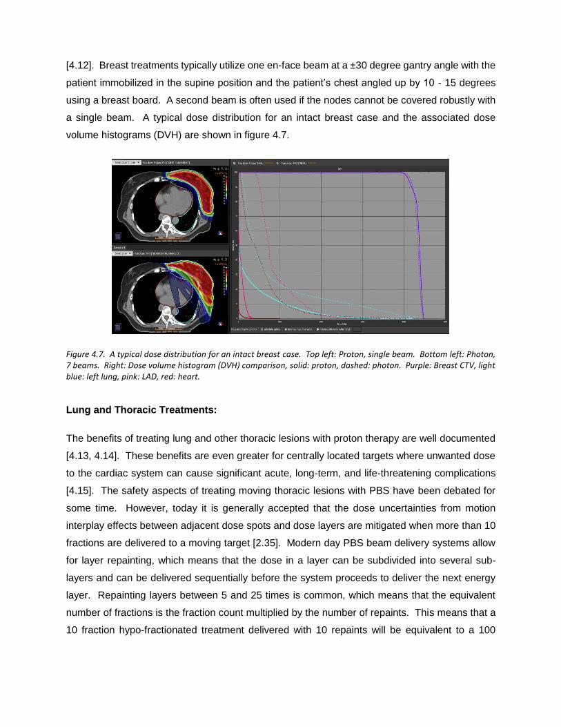
[4.12]. Breast treatments typically utilize one en-face beam at a ±30 degree gantry angle with the

patient immobilized in the supine position and the patient’s chest angled up by 10 - 15 degrees

using a breast board. A second beam is often used if the nodes cannot be covered robustly with

a single beam. A typical dose distribution for an intact breast case and the associated dose

volume histograms (DVH) are shown in figure 4.7.

Figure 4.7. A typical dose distribution for an intact breast case. Top left: Proton, single beam. Bottom left: Photon, 7 beams. Right: Dose volume histogram (DVH) comparison, solid: proton, dashed: photon. Purple: Breast CTV, light blue: left lung, pink: LAD, red: heart.

Lung and Thoracic Treatments:

The benefits of treating lung and other thoracic lesions with proton therapy are well documented

[4.13, 4.14]. These benefits are even greater for centrally located targets where unwanted dose

to the cardiac system can cause significant acute, long-term, and life-threatening complications

[4.15]. The safety aspects of treating moving thoracic lesions with PBS have been debated for

some time. However, today it is generally accepted that the dose uncertainties from motion

interplay effects between adjacent dose spots and dose layers are mitigated when more than 10

fractions are delivered to a moving target [2.35]. Modern day PBS beam delivery systems allow

for layer repainting, which means that the dose in a layer can be subdivided into several sub-

layers and can be delivered sequentially before the system proceeds to deliver the next energy

layer. Repainting layers between 5 and 25 times is common, which means that the equivalent

number of fractions is the fraction count multiplied by the number of repaints. This means that a

10 fraction hypo-fractionated treatment delivered with 10 repaints will be equivalent to a 100

fraction treatment, from a target motion perspective. This is another huge advantage that PBS

offers over IMRT, where this is simply not a practical solution.

Respiration gating for proton beam deliveries is easy, but to determine where the target is at any

given moment is not so easy. The other problem with gating, specifically in a multi-room proton

therapy center, is that it increases the treatment time in a treatment room which adversely affects

the throughput in other treatment rooms, since they are receiving the proton beam from the same

accelerator. To avoid the need for gating, it is common practice to define an internal target volume

(ITV) that covers the entire motion envelope of the gross tumor volume (GTV) and to treat the ITV

plus a certain margin to the desired dose. Due to the reduced integral dose with PBS, the volume

of lung that receives 20 Gy or less is often significantly less than even a gated photon beam

delivery, despite the fact that the ITV is significantly larger than the GTV. The next generation

proton therapy systems will allow for much faster inter-room beam switching and beam delivery

times, which allow for a more time efficient implementation of respiration gated treatments.

High-Risk Prostate Treatments:

High-risk prostate treatments regularly require that a significant portion of the pelvic nodes be

treated, in addition to the prostate gland and seminal vesicles. This results in an extremely

complex target shape with the small bowel, bladder, and rectum that must be spared.

Comparisons between PBS, planned with robust optimization, and VMAT for the treatment of

high-risk prostate cancer have been performed at PCPT to validate the use of PBS (MFO) for

high-risk prostate treatments. This study confirmed that robustly planned PBS significantly

reduced the dose to normal tissues in the pelvis while maintaining target coverage. Rectum and

bladder dose reduction with PBS may improve the therapeutic response beyond the levels

accomplished with VMAT [4.14].

Patients with high-risk prostate cancer are now treated on a routine basis at the PCPT facility,

targeting the prostate gland, seminal vesicles, and pelvic nodes to a dose of 46 - 50 Gy(RBE),

followed by a boost dose to the prostate gland for a cumulative dose of 78 Gy(RBE) using PBS.

Most importantly, suspicious or positive nodes can be boosted to a higher dose simultaneously

with the prostate boost to dose levels exceeding 60 – 66 GyRBE, depending on bowel proximity.

This is illustrated in figure 4.8, which shows a treatment plan for a high-risk nodal prostate

treatment.

The implementation of PBS also benefits low and intermediate risk prostate patients, but more so

for cases where the prostate droops significantly over the rectum and for patients with a hip

replacement. In those cases, PBS allows for shaping the beam over the rectum, which was not

possible with DS or US deliveries. The latest long-term outcome (median follow-up time of 5.5

years) data for prostate treatments, published by the University of Florida, revealed that the 5-

year freedom from biochemical progression (FFBP) rates were 99%, 94%, and 74% in low-risk,

intermediate-risk, and high-risk patients, respectively [4.15]. These treatments were performed

with DS beam delivery techniques.

Figure 4.8. A typical high-risk prostate plan employing two lateral fields. Each lateral field treats the nodes on that respective side and the entire prostate gland. The sum of these two fields constitutes the complex dose map shown in the bottom panel. Red = 46 Gy(RBE), Light green = 36.8 Gy(RBE)

In April 2015, Augmenix INC. introduced SpaceOAR hydrogel that is inserted between the anterior

rectal wall and the prostate, displacing the rectum away from the prostate [4.16, 4.17, 4.18]. The

gel insertion typically creates a space, occupied by the gel, ranging between 10 and 15 mm. PBS,

together with SpaceOAR, allowed for reducing the volume of the rectum receiving 90% of the

prostate dose to less than 1%, on average. At PCPT we have been using SpaceOAR since April

2015 on the majority of prostate patients. This technique further reduced the already low grade

1 and grade 2 toxicities previously experienced by the patients treated without SpaceOAR gel

and has so far totally eliminated any grade 3 acute toxicities.

Head and Neck Treatments:

Head and neck (H&N) cancers present one of the most complex shaped and challenging targets

to the Radiation Oncologist. In most cases, the lymph nodes on at least one side of the neck,

and often on both sides of the neck, need to be treated to doses higher than 60 Gy. Several

dosimetric studies were conducted to evaluate the feasibility of using PBS for these cancers [2.36,

4.19]. A general consensus is that in treating oropharyngel cancers, PBS reduces normal tissue

exposure, in particular the posterior pharynx and oral cavity, without sacrificing target coverage.

Treating patients for H&N cancers at many proton therapy institutions with PBS revealed that

these dosimetric advantages appeared to translate into lower rates of acute treatment-related

toxicity including mucositis, dysgeusia, and nausea, compared with IMRT [4.20]. Based on

discussions with physicians at PCPTK where we predominantly treat bilateral neck, I conclude

that the patients tolerate the H&N treatments generally well with acute toxicity not dissimilar to

IMRT but with more rapid and complete recovery of swallowing function, taste, and saliva. Weight

loss during treatment does occur and often requires adaptive plans, which are relatively easy with

PBS.

4.6. SUMMARY

The future of proton therapy is very promising. The immediate positive impact that PBS has had

on the clinical landscape is beyond reproach. Although this was evident since the first patients

were treated at the Paul Scherrer Institute (PSI) in 1996 [2.31], it became more evident when PBS

became a clinical reality in many more treatment centers across the globe. The clinical teams at

the University Medical Center in Groningen (UMCG) in the Netherlands, under the leadership of

Dr. Hans Langendijk, realized the advantages that PBS can bring to their clinical program. They

undertook an intensive investigation into the need for proton therapy at the UMCG, doing

retrospective analyses of normal tissue complication probabilities that occurred in several cohorts

of patients treated at the UMCG [4.21]. Figure 4.9 shows a bar graph (reproduced with permission

from Dr. Langendijk) of the projected future utilization of a PBS based proton therapy system at

UMCG. It is interesting to note that 75% of PBS utilization is for prevention of complications and

secondary cancers. Only 20% of the cases they plan to treat will aim at improving local control,

while only 5% will be for standard indications. The standard indications are more or less what

proton therapy has been used for until the clinical realization of PBS. In other words, the standard

indications in figure 4.9 represent the same indications listed on the left side of the dashed line in

figure 4.6. This means that the potential clinical benefit of PBS is far beyond what was expected

or predicted in the earlier days of proton therapy.

Figure 4.9. The projected clinical utilization of the UMCG proton therapy facility that is now under construction in Groningen, the Netherlands (Reproduced with permission from Dr. H Langendijk).

After many years of dedicated work from many people in the field of particle radiation therapy, we

have finally reached a stage that enables us to declare that proton therapy is now ready for mass

adoption in the clinical practice. This adoption is happening at a rapid pace. Arthur Schopenhauer

(1788-1860) stated that all truth passes through three stages. First, it is ridiculed; second, it is

violently opposed; and third, it is accepted as being self-evident. It is my opinion that the clinical

realization of PBS, together with many technological advances, has made it possible for proton

therapy to advance to the third stage of Schopenhauer’s hierarchy. We will continue to see a

near exponential growth in the number of proton therapy treatment vaults over the next decades.

This growth in proton utilization will, in turn, allow for reducing the costs and construction times

even further. The clinical realization of PBS allows for the exploitation of the full potential of

accelerated proton beams in the pursuit of increasing the therapeutic ratio. Bringing PBS to mass

clinical adoption is a true testimony of the importance of the radiation therapy technological

evolution that started with Roentgen’s discovery of x-rays in 1896.

CHAPTER 5:

WHAT IS NEEDED IN THE NEXT TEN YEARS TO ALLOW FOR THE

MASS ADOPTION OF PROTON THERAPY?

5.1. OVERVIEW

This chapter will address the need for continued improvements in proton therapy beam delivery

and general efficiencies. I make the argument that proton therapy systems can eventually become

much less expensive than current proton therapy systems – even to the cost level of modern

specialized x-ray systems such as the MRI Linac. Currently, proton therapy systems are still much

more expensive than electron and x-ray therapy systems because it is more expensive to

accelerate protons to clinically suitable energies and to transport and deliver the protons to the

patient, than it is for electrons and X-rays. Hence, the current proton accelerators and isocentric

gantry systems are still very large compared to electron accelerators and gantries used in x-ray

therapy. A multi-room proton therapy system requires a separate beam transport line to bring the

accelerated protons to the treatment room and the treatment vaults need to be very large to

accommodate the large gantry systems. All of this makes a proton system very expensive

compared to a typical state-of-the-art x-ray therapy system. The efficient operation of such

systems is therefore also paramount in order to make the currently installed clinical systems

financially viable, especially in the light of ever-increasing medical costs.

In this chapter, I start to present a peer reviewed, invited paper published in 2020 in the British

Journal of Radiology (BJR) as a special feature edition. I was honored to be asked by Professor

Tony Lomax to contribute a paper to this edition of the BJR on proton therapy beam delivery, with

specific focus on what is needed in the next ten years. All the authors were limited to a maximum

of 4000 words in their papers and therefore, I had to be extremely selective on what I believe are

the top priorities of what needs to be implemented and developed over the next ten years.

Figure 5.1: A simplified external beam radiation therapy process flow diagram.

The BJR paper only addresses beam delivery aspects which are often tightly related to patient

positioning and position monitoring aspects. Compiling this paper required in-depth research and

knowledge of technologies that have been developed but not implemented or that are being

developed that should be implemented over the next ten years. The process flow for an external

beam radio therapy treatment is shown in Figure 5.1. The upper control track deals with the

preparation and control of the beam used in delivering the dose to the target. The bottom control

track deals with getting the patient positioned for treatment and ensuring that the patient remains

in the correct position during beam delivery. In the past, all research and development funding

has gone into the beam delivery aspects of a radiotherapy system, with little going into imaging

and positioning the patient for treatment. However, during a cancer treatment session more than

90% of the time is spent on positioning the patient and comforting them.

Two main aspects that I was not able to address in the paper are optical guidance and the

possibility to treat the patients in an upright position eliminating the need of large and expensive

gantries. I will briefly address these and indicate how this will improve efficiencies in the proton

therapy workflow.

The details of the BJR paper publication dates and author list are shown in Figure 5.2. I invited

Dr. Jacob Shamblin to co-author this paper. Dr Shamblin is a nuclear physicist working at

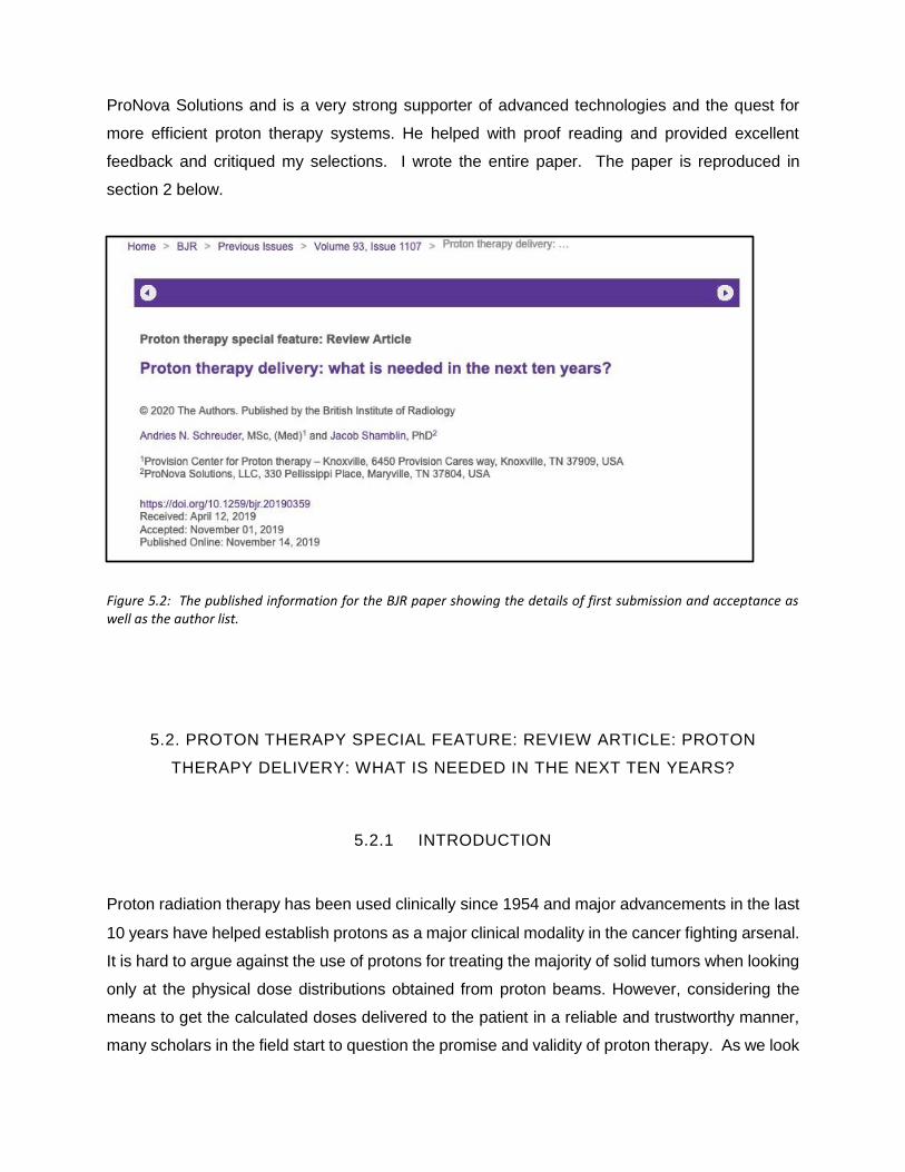
ProNova Solutions and is a very strong supporter of advanced technologies and the quest for

more efficient proton therapy systems. He helped with proof reading and provided excellent

feedback and critiqued my selections. I wrote the entire paper. The paper is reproduced in

section 2 below.

Figure 5.2: The published information for the BJR paper showing the details of first submission and acceptance as well as the author list.

5.2. PROTON THERAPY SPECIAL FEATURE: REVIEW ARTICLE: PROTON

THERAPY DELIVERY: WHAT IS NEEDED IN THE NEXT TEN YEARS?

5.2.1 INTRODUCTION

Proton radiation therapy has been used clinically since 1954 and major advancements in the last

10 years have helped establish protons as a major clinical modality in the cancer fighting arsenal.

It is hard to argue against the use of protons for treating the majority of solid tumors when looking

only at the physical dose distributions obtained from proton beams. However, considering the

means to get the calculated doses delivered to the patient in a reliable and trustworthy manner,

many scholars in the field start to question the promise and validity of proton therapy. As we look

at the road ahead of us from a proton beam delivery perspective, the authors believe we now

have the means to make proton therapy highly effective through efficient beam delivery and

patient positioning technologies. Technologies will (and should) always evolve but we believe

enough major breakthroughs have been accomplished over the last 10 years to allow for a major

revolution in proton therapy beam delivery aspects. This paper will address the major technology

advancements that are now ready for mass implementation in the proton therapy space and will

encourage vendors to bring these to market to benefit the cancer population worldwide.

5.2.2 DELIVERY MODALITIES

The paper is a forward-looking review of how proton therapy systems should operate 10 years

from now. Other authors will address the needs with respect to treatment planning, biological

modeling, patient positioning and socio-economic aspects. However, proton beam delivery

cannot be addressed without also addressing patient positioning aspects. We will discuss patient

positioning only in the context of achieving better and more efficient beam delivery. We will also

discuss how these technologies impact the design aspects of future proton beam delivery

systems.

The following is a list of “must-haves” from a beam-delivery perspective for a proton therapy

system circa 2030.

Prerequisites for a Proton system in 10 years

1. Proton arc therapy.

2. Rapid beam delivery enabling FLASH therapy

3. Proton beam-based image guidance - in vivo range verification and proton beam imaging.

4. On-line adaptive therapy – “on the fly”. Bring the beam to the patient.

5. Beam control based on the patient’s respiration cycle – full 4D beam delivery.

6. Fast trimming apertures.

7. Beam focusing conditions – variable spot size.

8. System self-diagnostics and self-calibration – automatic warm-up and checking overnight.

The majority of the prerequisites listed above have been described extensively in recent years by

many experts in the field. We will only cite a representative sample of these reviews and not

discuss the technologies per se. The reader is encouraged to read these papers to obtain further

details.

5.2.2.1. Arc therapy.

The use of arc therapy was first proposed for photon beams in 1965 by Takahashi et al. and

further developed by pioneers like Brahme and Yu [5.1, 5.2, 5.3, 5.4]. In 1997, Deasy et al.

proposed the use of arc therapy in protons using the distal edge tracking principle [5.5]. Although

the clinical value was very well appreciated, this was initially dismissed from both a technology

perspective and a range uncertainty point of view [5.6]. It was not until the first Tomotherapy®

units, proposed in 1993 by Mackie, were used clinically that the value of arc therapy, specifically

from a dose conformity index, was realized for the photon-space [5.7, 5.8, 5.9, 5.10].

Figure 5.3. A robust optimized IMPT treatment plan for a prostate (A) compared to a SPArc plan (B). The dose distribution advantages are illustrated in the DVH (C) and dose difference (D) panels. (Used with permission from Ding et al.16)

Technological developments sparked new interest in proton arc therapy since 2013 and several

groups reported on the benefits of such beam delivery techniques [5.11, 5.12, 5.13, 5.14]. Ding

et al. recently showed the feasibility of delivering continuous spot-scanning proton arc (SPArc)

therapy to a phantom at the William Beaumont Hospital proton therapy center using an IBA

Proteus®ONE system (Ion Beam Applications S.A., Louvain-La-Neuve, Belgium) [5.15, 5.16].

The dosimetric benefits of proton arc therapy is shown in Figure 5.3. A significant reduction in

beam delivery time when using SPArc has also been demonstrated by Ding et al [5.16].

The increased benefit from protons is immediately evident when comparing Intensity Modulated

(x-Ray) Radiation Therapy (IMRT), in which the beam intensity can only be modulated

transversely, with a proton beam where it can be controlled in all three dimensions. The “range

uncertainty problem” (i.e., where the proton beam actually stops) is soon to be reduced to a

clinically insignificant problem or even eliminated when proton radiography and proton

tomography are used to map out the real tissue stopping powers within the patient (see next

section on in vivo measurements) [5.17]. With the stopping point known to a high degree of

accuracy, the treatment planning system (TPS) can optimize the dose per useable spot for each

beam in the arc. It’s important to note that the TPS is not using distal edge tracking per se but

rather the best spots for the best results. It is also easy to build the linear energy transfer (LET)

distribution into the optimization process to ensure higher LET regions are moved away from more

biologically sensitive structures [5.18, 5.19].

Future proton therapy systems must be designed to provide enough free space around the patient

to facilitate a collision-free rotation while maintaining the desired beam characteristics. The beam

delivery systems must also be able to deliver continuous beams at variable intensities while

rotating. Gating or synchronizing the beam delivery with the patient’s respiration cycle for thoracic

and abdominal targets is also essential.

5.2.2.2. Fast beam delivery - FLASH therapy

FLASH radiation therapy is defined as delivering the radiation at dose rates in excess of 40 Gy/sec

with the rationale that healthy tissue is spared at such high dose rates [5.20, 5.21]. The exact

biological mechanisms of FLASH radiation are not yet fully understood but scientists believe that

one possible mechanism might be that the tissue exposed to FLASH radiation becomes deprived

of oxygen and thus becomes radio-resistant. This has been shown in several small animal

experiments [5.22]. The principle of FLASH radiation is that the healthy tissues must still receive

less radiation than the target but at a very high dose rate [5.23]. One of the primary reasons for

fractionated treatments is to allow the healthy tissues to recover from unwanted damage. FLASH

radiation will allow for a significant reduction in the number of treatment fractions since the healthy

tissues are spared. Several groups are now actively working on techniques on delivering FLASH

radiation and Phase I clinical trials are being planned to start within the next three years (Dee

Khuntia MD. Chief Medical Officer, Varian Medical Systems. Personal communication. 27th

March 2019). The authors believe that a form of arc proton therapy might be the easiest way to

deliver FLASH radiation as the healthy tissue is only traversed once. Ordinary pencil beam

scanning likely cannot be used for this purpose since the healthy tissue gets exposed each time

during dose delivery to a given layer. The ability to introduce ultra-fast energy changes will help

to deliver FLASH radiation since it will allow for fast scanning in the depth dimension, delivering

a tube of high dose rather than a single spot, i.e. “tube scanning”. The length of the “tube of dose”

is tailored to the extent of the target in depth [5.24, 5.25].

In order to be able to deliver FLASH proton therapy future systems must be able to measure the

delivered dose accurately at the required high dose rates. The need for highly accurate patient

positioning is obvious as the number of treatment fractions will be reduced dramatically.

5.2.2.3. Proton beam-based image guidance – in vivo range verification and proton beam

imaging.

One of the benefits of proton therapy is the presence of nuclear interactions that generate

secondary radiation. This secondary radiation can in turn be measured to obtain valuable

information related to the proton interactions inside the patient’s body. This is referred to as in

vivo range verification and techniques required to facilitate this have been reviewed extensively

by Knopf et al. and Parodi et al [5.26, 5.27]. The most documented and researched options

involve measuring the prompt gamma radiation emitted as the beam penetrates the tissue and

the gamma rays when positrons from certain beta-emitting isotopes of interest annihilate near

their point of origin. The latter is referred to as positron emitted tomography (PET). When first

postulated for clinical use it was believed that this PET activity could also be used to accurately

determine the dose delivered, but this objective turned out to be difficult to implement in practice.

Modern treatment planning dose calculation algorithms can calculate the absolute dose delivered

accurately enough but still struggle to calculate the range primarily due to the uncertainties in the

Hounsfield-unit to stopping power conversion [5.20, 2.40]. The most attractive feature of these

techniques is to detect acute changes in the patient’s anatomy, e.g. changes in the content of

sinus cavities that can cause drastic changes in the depth of penetration. Analyzing the energy

spectra of the prompt gamma radiation allows for identifying the elemental composition of the

radioactive tissue. This knowledge yields additional advantages. This work is ongoing and has

been demonstrated by Hueso-González et al. [5.28]. Implementing prompt gamma imaging in

the clinical setting appears to be easier than PET methods mainly due to problems with biological

washout and the fact that the cross section for PET isotope production decreases rapidly with

decreasing proton energy, particularly in the region where the protons are stopping, which

substantially decreases the accuracy of proton range estimation [5.26, 5.27].

A complementary technique to reduce range uncertainty involves using the proton beam itself

rather than secondary radiation. The use of proton radiography (pRad) was proposed in the 1960s

with the first proton radiographs being published in 1968 by Koehler using the proton beam at the

Harvard Cyclotron facility [5.29]. Cormack, who shared the Nobel Prize with Hounsfield for

inventing the CT scanner, worked with Koehler and reported on proton Computed Tomography

(pCT) in 1976 [5.30]. Similar to x-ray CT, pCT images can be reconstructed from a series of

adequately spaced pRad images. The use of proton radiography to improve the dose calculation

accuracy in proton beams was demonstrated by Schneider in 1996 at the Paul Scherrer Institute

in Switzerland [5.31]. The development of pRad was stalled for many years as it was believed

that pCT is only possible at proton energies above 250 MeV to traverse the patient’s body for all

anatomical sites. However, pRad images can play a very important role for a large percentage

of cases treated with 230 MeV beams, especially in the cases where setup and range accuracy

are more important. In these cases, the beams must stop before reaching critical structures (e.g.,

the optic chiasm or brainstem), but anatomical changes or complex anatomy, often further

impacted by pre-treatment surgical procedures, make it difficult to properly account for range

uncertainties which can change even during the course of the treatment. A team of researchers

from the Chicago Proton Therapy Center recently reported on a study showing that 96.8% and

94.7% of proton beams used to treat head and neck and thoracic cases at that facility would have

been able to traverse the patients with at least 2 cm of residual range left to facilitate a pRad

image [5.32].

A pCT image data set is composed of the measured proton stopping powers in the patient’s body

and therefore solves one long-standing issue in proton therapy i.e. the uncertainties in stopping

powers derived from electron densities obtained via x-ray imaging [2.39]. A pRad image is a direct

measurement of cumulative stopping powers along the ray lines from the proton source to the

respective point in the pRad imaging plane. Several pRad and pCT imaging systems are currently

under development and several groups have already reported on actual pRad and pCT images

on animals and anthropomorphic phantoms [5.17]. The range accuracy beyond the imaged object

is on the order of 0.2 mm. This is illustrated in Figure 5.4 which shows a proton radiograph of a

CATHPHAN line pair phantom obtained with the ProtonVDA system at our institute [5.33]. A

0.2mm-thick plastic tape that was used to hold the phantom in the beam is clearly visible in the

image. It is obvious that a single pRad image, like an x-ray image, will provide enough information

to align the patient along the beam axis. However, as an out-of-plane rotation will change the

proton range through the patient’s body, it is expected that a single pRad image may also contain

enough information to reasonably correct for out of plane rotations thanks to the high accuracy of

excess range detection.

Figure 5.4. A proton radiograph of a CATHPHAN line pair phantom obtained with the ProtonVDA system at our facility. A 0.2mmthick plastic tape used to hold the phantom in place is clearly visible in the image: See the diagonal (horizontal) streak across the image.

The spatial resolution of pRad images will probably always be weaker than that for x-ray images

due to Coulomb scattering in the patient [5.33]. However, Pankuch et al. also reported on a study

to investigate whether the spatial resolution of pRad images obtained with current state-of-the-art

systems is adequate for patient positioning. Their study employed the use of pRad images

calculated with known shifts and rotations with respect to a reference pRad image. A team of

independent experts then used 2D image registration techniques, equivalent to what is used in

daily patient setups, to derive the applied shifts and rotations. The same process was repeated

using reference and shifted x-ray images. The study revealed that the experts could obtain the

corrections within clinically acceptable tolerances, i.e. less than 1 mm translations and 0.5 degree

rotations. The differences in corrections obtained using x-ray and pRad images was statistically

insignificant [5.32].

Future proton therapy systems must be designed to enable the deployment of in-vivo dosimetry

equipment about the patient prior to (proton imaging) or during beam delivery (prompt Gamma or

PET) without impacting the patient’s position or comfort (e.g. claustrophobia). Proton imaging

also requires extremely low beam intensities which means that the beam delivery systems must

be able to delivery low beam currents in the order of 3 x106 protons per second over a 20 x 20

cm2 area accurately and safely [5.34]. Achieving these milestones will then pave the way to bring

on-line adaptive therapy into the clinical proton therapy space.

5.2.2.4. On-line adaptive therapy – on the fly. Bring the beam to the patient.

The standard practice in radiation therapy is to use x-ray-based imaging techniques only to

determine where the patient is with respect to the radiation beam and then send a 6-dimensional

correction vector to the patient positioner system (PPS) to move the patient into the desired

position for treatment. This is referred to as “bringing the patient to the beam”. Proton therapy

provides an exciting opportunity to reverse this process. Using pRad or pCT images provides

adequate information to recalculate the proton beams (either static beams or arcs) according to

the patients existing position and anatomy. There is pushback within the community against

recalculating an adaptive plan without formal verification (i.e. patient specific QA). However, the

new beams can be easily verified with a low dose pRad image prior to delivering the beam [5.32]

and there is a point that is often overlooked: an adapted plan is not a new plan [5.35]. The previous

beams must serve as the baseline for the adapted plan. Several parameters such as the total

imparted energy (total monitor units), the maximum beam energy, and the total number of layers

should be used as a baseline to ensure that the adapted beam is similar to the original beam. We

tested this proposal with a two-field mediastinal plan. The isocenter was shifted by 10 mm in all

three directions and a roll of 1 degree was introduced. The beams were reoptimized to the same

dose constraints and objectives. The total number of monitor units (MU) increased by 0.8% and

0.34% for two beams respectively. The change in the number of MU per energy layer for one of

the beams is illustrated in Figure 5.5. This shows that after adapting the beams for a relatively

large displacement from isocenter the beam parameters for both beams did not change

significantly. This could serve as a safety benchmark for real-time beam adaptations.

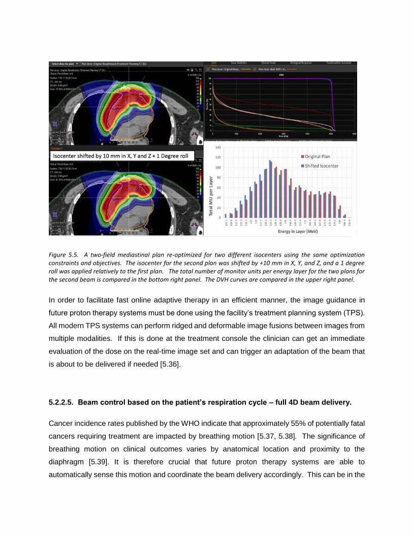
Figure 5.5. A two-field mediastinal plan re-optimized for two different isocenters using the same optimization constraints and objectives. The isocenter for the second plan was shifted by +10 mm in X, Y, and Z, and a 1 degree roll was applied relatively to the first plan. The total number of monitor units per energy layer for the two plans for the second beam is compared in the bottom right panel. The DVH curves are compared in the upper right panel.

In order to facilitate fast online adaptive therapy in an efficient manner, the image guidance in

future proton therapy systems must be done using the facility’s treatment planning system (TPS).

All modern TPS systems can perform ridged and deformable image fusions between images from

multiple modalities. If this is done at the treatment console the clinician can get an immediate

evaluation of the dose on the real-time image set and can trigger an adaptation of the beam that

is about to be delivered if needed [5.36].

5.2.2.5. Beam control based on the patient’s respiration cycle – full 4D beam delivery.

Cancer incidence rates published by the WHO indicate that approximately 55% of potentially fatal

cancers requiring treatment are impacted by breathing motion [5.37, 5.38]. The significance of

breathing motion on clinical outcomes varies by anatomical location and proximity to the

diaphragm [5.39]. It is therefore crucial that future proton therapy systems are able to

automatically sense this motion and coordinate the beam delivery accordingly. This can be in the

form of active gating, synchronization, or active target tracking [5.39]. Audiovisual guidance is

essential in this regard. Keall et al. recently reviewed 27 papers addressing motion management

and found that 21 of these papers indicated an advantage for audio or visual guidance. The best

results were observed when both audio and visual cues were offered to the patient to help with

stabilizing or controlling their breath rates [5.40]. Several methods can be used to track the

breathing motion, but one that holds significant promise in this regard employs an infrared camera

to measure the temperature of the air entering and exiting the patient’s nostrils [5.41, 5.42]. That

information can be used to quantify the tidal volume of air exchange that can be accurately

correlated to the breathing phase and in turn synchronize the beam delivery [5.41]. This should

be supplemented with surface rendering systems that can monitor for unwanted or involuntary

patient motion during treatment.

There are many third-party systems that perform motion and respiration monitoring, but future

systems should focus on integrating these into the control system architecture to enhance

workflow efficiencies making respiration monitoring readily available per the physician’s

prescription or the clinician’s judgement [5.43].

5.2.2.6. Fast trimming apertures

Pencil beam scanning revolutionized proton therapy from a usability and dose conformation

perspective but the penumbra for shallower beams delivered via PBS is significantly larger than

when the beam is shaped with an aperture [5.44]. Monte Carlo calculations now allows for

accurate dose calculations of pencil beam scanning with edge-sharpening apertures. The

benefits of a sharper penumbra are well documented in many clinical cases, especially where the

edge of the beam is in close proximity of a critical structure (e.g. parotid gland and the brainstem).

Static beam-shaping apertures are a workflow impediment and can only shape the edge of the

beam in the outer-most extent of the target. Hyer et al. proposed the use of fast-moving leaves

that can trim the spots on the beam edge for every layer being delivered [5.45, 5.46]. Mevion

recently introduced a very innovative adaptive aperture into clinical practice [5.47]. Adding such

a trimmer to more traditional beam delivery nozzles with smaller spot sizes than the Mevion

system will combine the benefits of small pencil beam scanning with a sharp penumbra and will

improve the conformity index for shallow targets. The improvement in penumbra obtained with

using an aperture for classical PBS beams within air spot sizes in the order of 3 mm sigma at the

highest energy, is shown in Figure 5.6 [5.48]. As can be seen from Figure 5.4, the aperture or

trimmer blades only improves the penumbra for ranges less than 17.5 cm. The thickness of the

trimmer blades used for these beams can therefore be reduced providing the use of the trimmer

is interlocked for higher energies. This will reduce the weight and improve the dynamics of such

devices.

Figure 5.6. Penumbra (P) as a function of proton range (R) for a spot-scanning beam with MLC collimation and uniform spot weights (square) and for spot scanning beam without MLC and variable spot weight (circle). Data are provided for three Bragg peak depths (4, 10 and 20 cm) corresponding to proton energies of 72, 118 and 174 MeV, respectively. Analytical fits to the data are provided in order to estimate the crossing point at R = 17.5 cm, corresponding to a proton energy of 159 MeV. (Used with permission from Bues et al. [5.48])

5.2.2.7. Beam focusing conditions – variable spot size.

As explained above, the proton beam penumbra for shallow targets are not optimal due to the

size of the beam spot [5.44, 5.48]. One method to overcome this is to use a smaller spot size on

the edge of the beam and larger spots in the center of the target by changing the beam focus as

required. This will allow for a sharper beam edge while reducing the risk of dose inhomogeneities

in the target due to potential spot position inaccuracies. It will also reduce the number of spots

required to fill the target which will reduce the beam delivery time. Vendors are reluctant to

implement this as it is technically challenging to install additional focusing elements, specifically

in gantry systems where space is restricted. Verifying the beam focus condition with the desired

accuracy is also challenging. One method that was recently proposed by Meier et al. is to first

deliver the spots on the edge of the beam with a small spot and then defocus the beam to a larger

spot and fill in the spots in the rest of the target [5.49, 5.50].

5.2.2.8. System self-diagnostics and self-calibration – automatic warm-up and checking

overnight.

Artificial intelligence (AI) and automation must play a much larger role in modern and new proton

therapy systems [5.51]. While a proton system is indeed fully automated, we are still doing

manual quality assurance checks by putting various external detectors in the beam merely to

measure again what the control system just measured during beam delivery. Modern systems

are already equipped with collision avoidance systems that prevents any mechanical collisions

between hardware components of the system [5.52]. By simply putting a test object on the

treatment couch, the entire system can be put in QA mode and it can cycle through checks during

the night shift when patients are not treated. The control system can steer the beam

systematically onto beam position monitors and test that the interdependencies of the different

monitoring circuits are intact. The image guidance system can interact with optical tracking

systems to ensure that all the systems involved in patient positioning are tracking with each other.

5.2.3. DISCUSSION

To look at the 2030 proton therapy landscape from a practical perspective we must consider three

pathways:

1. Existing (legacy) facilities still in operation;

2. New facilities that will be developed using traditional approaches and employing

single or multiple rooms from one accelerator;

3. New facilities that will not be bound by existing paradigms.

When looking at the prerequisites listed above its clear that it will be expensive to retrofit existing

facilities with many of the features on the list, but we argue that such facilities should at least be

capable of being retrofitted with features listed in Table 6.1.

Several vendors developed third generation proton therapy systems during the last decade as

recently reviewed by Farr et al [5.53]. The biggest problem with upgrading existing facilities is

that in most cases the system will have to be taken out of service for extended periods of time.

This is extremely expensive and adds to the total cost for the upgrade.

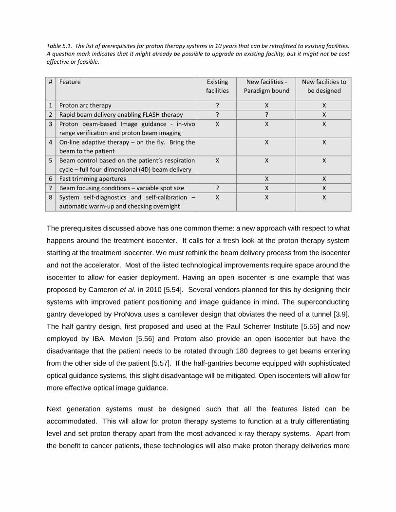
Table 5.1. The list of prerequisites for proton therapy systems in 10 years that can be retrofitted to existing facilities. A question mark indicates that it might already be possible to upgrade an existing facility, but it might not be cost effective or feasible.

# Feature Existing

facilities

New facilities -

Paradigm bound

New facilities to

be designed

1 Proton arc therapy ? X X

2 Rapid beam delivery enabling FLASH therapy ? ? X

3 Proton beam-based Image guidance - in-vivo

range verification and proton beam imaging

X X X

4 On-line adaptive therapy – on the fly. Bring the

beam to the patient

X X

5 Beam control based on the patient’s respiration

cycle – full four-dimensional (4D) beam delivery

X X X

6 Fast trimming apertures X X

7 Beam focusing conditions – variable spot size ? X X

8 System self-diagnostics and self-calibration –

automatic warm-up and checking overnight

X X X

The prerequisites discussed above has one common theme: a new approach with respect to what

happens around the treatment isocenter. It calls for a fresh look at the proton therapy system

starting at the treatment isocenter. We must rethink the beam delivery process from the isocenter

and not the accelerator. Most of the listed technological improvements require space around the

isocenter to allow for easier deployment. Having an open isocenter is one example that was

proposed by Cameron et al. in 2010 [5.54]. Several vendors planned for this by designing their

systems with improved patient positioning and image guidance in mind. The superconducting

gantry developed by ProNova uses a cantilever design that obviates the need of a tunnel [3.9].

The half gantry design, first proposed and used at the Paul Scherrer Institute [5.55] and now

employed by IBA, Mevion [5.56] and Protom also provide an open isocenter but have the

disadvantage that the patient needs to be rotated through 180 degrees to get beams entering

from the other side of the patient [5.57]. If the half-gantries become equipped with sophisticated

optical guidance systems, this slight disadvantage will be mitigated. Open isocenters will allow for

more effective optical image guidance.

Next generation systems must be designed such that all the features listed can be

accommodated. This will allow for proton therapy systems to function at a truly differentiating

level and set proton therapy apart from the most advanced x-ray therapy systems. Apart from

the benefit to cancer patients, these technologies will also make proton therapy deliveries more

efficient with obvious operational benefits. The latter will help with justify the higher costs of proton

therapy systems.

5.3. OPTICAL GUIDANCE TO SUPPLEMENT 3D VOLUMETRIC IMAGE

GUIDANCE.

Cone Beam CT (CBCT) finally made it into proton therapy image guidance and is now a standard

tool in all modern proton therapy systems. However, one of the main benefits of proton therapy

is the reduced integral dose which is somewhat compromised with the low dose bath from regular

repeat CBCT acquisitions. One of the most neglected areas in proton therapy is optical guidance

to supplement CBCT volumetric imaging.

Optical tracking technologies have been developed over the last few decades and are heavily

used in automation [5.58]. The most notable developments over the last few years were in

autonomous (self-driving) vehicles which rely on global position techniques, but also on optical

analyses of the immediate surroundings [5.59]. Such techniques must be used in positioning the

patient for external beam radiation therapy. Surface rendering techniques are used in surface

guided radiotherapy (SGRT) and such systems are commercially available and are mainly used

in hypo fractionated treatments and breast treatments [5.60, 5.61]. These systems also provide

a gating signal that can be used to synchronize the beam delivery with the patient’s breathing

cycle. It is my opinion that these systems are moving in the right direction but can be made much

more intelligent in order to play a bigger role in patient setup. One example would be to have the

optical tracking systems fully integrated with the Oncology Information system to automatically

use the information obtained during the CT scanning process for the first treatment setup and the

treatment setup information for the next treatment and so on. Three-dimensional (3D) camera

systems are also used extensively in automation and rapid prototyping. Such systems could also

be installed in modern treatment rooms to obtain a 3D surface of the patient’s body in the

treatment region and this could be compared with the 3D surface obtained from the skin contour

of the CT data set. Any changes in the patient’s 3D posture can then be discovered and corrected

prior to any patient setup activities. 3D cameras can also be used in real time for motion tracking

as well as the detection of unwanted motions and baseline shifts. Another very promising

development, discussed earlier in this chapter (see section 2.2.4), is in the use of thermal cameras

to measure the air volume and temperature entering and exiting through the patient’s nostrils

while breathing.

5.4. THE CASE FOR UPRIGHT TREATMENTS

Perhaps the most neglected and the most obvious aspect that can lead to enormous cost savings

and efficiency enhancements is to do away with expensive proton therapy gantry systems. As

discussed in chapter 2, employing fixed horizontal beams has been exploited in early systems to

treat the patients in a seated position [1.9, 1.10] and at Fermi Lab, patients were treated in an

upright position with neutrons [5.62, 5.63]. This was always regarded as a suboptimal

arrangement that was forced on proton therapy when it was only available in physics research

institutions, before the very large, expensive gantry systems were developed. I am convinced

that the need for proton gantries comes from the fact that gantries were needed for neutron

therapy. When the neutron therapy clinical results struggled to live up to the promises in the early

eighties, people in the field reasoned that it is because they could not achieve the same

conformality in dose. This was mainly due to the lack of neutron beam gantries and not having

multileaf collimators to allow for beam shaping to conform the beams to the target. That argument

led to the development of isocentric neutron gantries and multileaf collimators. A multileaf

collimator was installed in the Louvain-laNeuve Facility in Belgium [5.64] and the University of

Washington neutron therapy facility in Seattle [5.65], while a multi-rod collimator was developed

for the Harper Grace neutron therapy facility in Detroit [5.66]. This notion was justified and

partially correct since neutrons are neutral particles and exhibit similar beam characteristics as

photons, requiring many conformal beams to improve the conformity index. I am convinced that

this argument – apples to apples vs apples to oranges – was the main driver behind the need for

proton gantries.

The proton depth dose curve (Bragg Peak) allows for a totally different paradigm in delivering the

dose to a target. The fact that the beam stops and that fewer beams are typically used in proton

treatment plans, defeats the argument that proton gantries are essential. This paradigm is finally

shifting. Treatment systems designed to treat patients in an upright orientation will fit in existing

xray therapy system vaults, obviating the need for new and larger radiation shielding vaults and

reducing the total costs dramatically.

The general consensus today is that it’s better to treat the patient in the same position as the

patient was scanned mainly due to the displacement of organs when the patient is moved from a

lying to an upright position. Only intracranial lesions could be treated in an upright position when

scanned in a lying position. Due to the lack of scanners that could scan the patient in an upright

position clinician therefore started to believe that patients are simply better treated in a lying

position. Multimodality imaging is an important aspect of treatment planning and target

delineation. The best registration between different modality images is obtained with the patient

in the same orientation when the imaging is done. Like CT scanners all other imaging systems

i.e. PET, MRI, PET-CT, gamma Cameras and even Ultrasound scans are designed to image the

patient in a lying position. This notion further supports the thinking that radiation therapy

treatments should be done in the lying position.

5.4.1. The clinical benefits of upright treatments

The traditional clinical concerns around upright treatments are outweighed by the potential

benefits that upright treatments hold for many patients. The advantages of treating the patient in

a seated or upright position has been systematically addressed by several scholars in the field.

Verhey et. al. reported in 1981 that patients can be immobilized effectively in the seated position

with less unwanted motions than in a supine or decubitus position [5.67]. McCarroll et. al. reported

on the benefits of treating thoracic and Head and neck patients in a seated position [5.68]. Yang

et. al. reported that thoracic patients breathe easier and are more relaxed in an upright position

while the lung volume is on average 25% larger compared to the supine position and the excursion

of a lung tumor as a result of breathing motion is also smaller [5.6971]. The WHO reported

recently that 55% cancer deaths are from disease sites that are affected by breathing motion

[5.38]. It is easy to conclude that treating these cases in a seated or upright position will result in

improved patient comfort, less target motion and less lung volumes being irradiated.

One of the main benefits of having the patient immobilized in an upright position is the reduced

risk of asphyxiation. The need to swallow which causes significant movement in the Neck and

esophageal regions are also significantly reduced [5.68]. Applying anesthesia to patients

immobilized in the upright position might also be safer with respect to the risk of asphyxiation

providing a proper support system for such patients are developed.

5.4.2. Other benefits of upright treatments

The technical benefits of upright treatments are numerous, but I will not elaborate on these in

great detail in this thesis. Rotating a 100 to 250 Kg patient isocentrically is certainly much easier

than moving a more than 50 ton gantry around the patient with the required precision. This of

course means that one need to focus on patient comfort and proper immobilization of the patient

in the upright position. Cone beam CT (CBCT) images of the patient can easily be obtained while

rotating the patient precisely in a stationary x-ray beam measuring the transmission x-rays with

stationary x-ray detectors. Proton radiography (P-Rad) and proton computed tomography (PCT)

images can be obtained in a similar manner providing the proton beam energy is sufficient for the

protons to traverse the specific anatomical region. Upright treatments require only fixed beam

lines which will allow for moving the scanning magnet further away from the isocenter. This in

turn will allow for faster beam scanning since less scanning power is required. The benefits of

faster scanning are important in terms of organ motion and FLASH radiation therapy (see section

2.2.2 above). Other benefits of moving the scanning magnet further away from the isocenter are

a larger source to axis distance (SAD) and the ability to scan the beam to larger field sizes. If a

fixed beam delivery nozzle is equipped with a collapsible vacuum section or a helium bag smaller

spot sizes can be achieved. This will also allow for variable spots sizes since the beam control

does not have to accommodate variations in the beam optics as a result of changes in the gantry

angle. Implementing fast trimmer apertures as discussed in section 2.2.6 above will also be much

easier since the gravitational forces on the trimmer components will be constant. The treatment

envelope around the patient is much is also more accessible and predictable in a fixed beam

arrangement. It is evident that all the prerequisites for a proton therapy system discussed in the

BJR paper above are much more attainable in a fixed beam configuration.

The benefits of upright treatments in reducing the cost of a proton therapy system are self-evident.

Fixed beams are cheaper to construct and much easier to maintain as they comprise of fewer

components. Installing and commissioning fixed beam systems will also be faster which will result

in significant project cost savings. The shielded volume for a fixed beam system is much smaller

and the wall thicknesses can be reduced significantly over the bulk of the shielded volume since

the primary beam will only be directed in one direction. This will allow for optimizing the treatment

room layout without significant cost ramifications. The latter will also allow for improved treatment

workflow and throughput efficiencies.

5.4.3. Upright patient positioning and imaging

As discussed in chapter 2, I proposed the use of an inclined beam system in 1998 and 8 such

treatment rooms were constructed by IBA and Procure [3.25, 5.54]. The inclined beam line

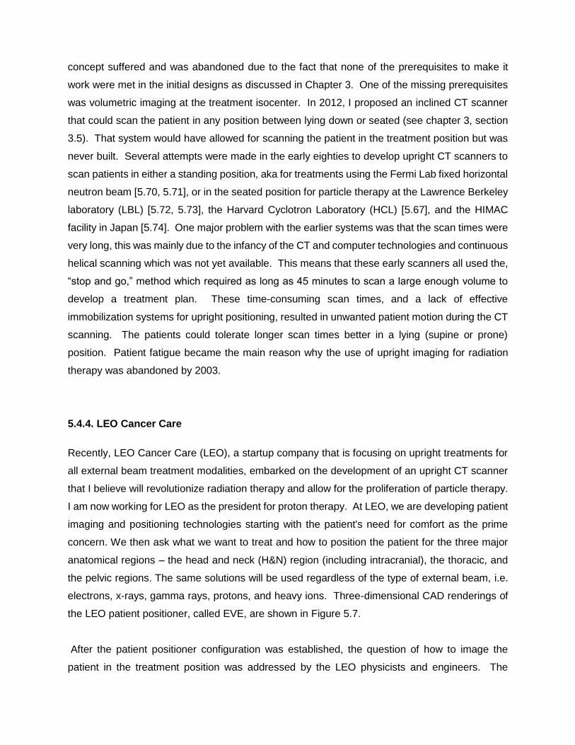
concept suffered and was abandoned due to the fact that none of the prerequisites to make it

work were met in the initial designs as discussed in Chapter 3. One of the missing prerequisites

was volumetric imaging at the treatment isocenter. In 2012, I proposed an inclined CT scanner

that could scan the patient in any position between lying down or seated (see chapter 3, section

3.5). That system would have allowed for scanning the patient in the treatment position but was

never built. Several attempts were made in the early eighties to develop upright CT scanners to

scan patients in either a standing position, aka for treatments using the Fermi Lab fixed horizontal

neutron beam [5.70, 5.71], or in the seated position for particle therapy at the Lawrence Berkeley

laboratory (LBL) [5.72, 5.73], the Harvard Cyclotron Laboratory (HCL) [5.67], and the HIMAC

facility in Japan [5.74]. One major problem with the earlier systems was that the scan times were

very long, this was mainly due to the infancy of the CT and computer technologies and continuous

helical scanning which was not yet available. This means that these early scanners all used the,

“stop and go,” method which required as long as 45 minutes to scan a large enough volume to

develop a treatment plan. These time-consuming scan times, and a lack of effective

immobilization systems for upright positioning, resulted in unwanted patient motion during the CT

scanning. The patients could tolerate longer scan times better in a lying (supine or prone)

position. Patient fatigue became the main reason why the use of upright imaging for radiation

therapy was abandoned by 2003.

5.4.4. LEO Cancer Care

Recently, LEO Cancer Care (LEO), a startup company that is focusing on upright treatments for

all external beam treatment modalities, embarked on the development of an upright CT scanner

that I believe will revolutionize radiation therapy and allow for the proliferation of particle therapy.

I am now working for LEO as the president for proton therapy. At LEO, we are developing patient

imaging and positioning technologies starting with the patient's need for comfort as the prime

concern. We then ask what we want to treat and how to position the patient for the three major

anatomical regions – the head and neck (H&N) region (including intracranial), the thoracic, and

the pelvic regions. The same solutions will be used regardless of the type of external beam, i.e.

electrons, x-rays, gamma rays, protons, and heavy ions. Three-dimensional CAD renderings of

the LEO patient positioner, called EVE, are shown in Figure 5.7.

After the patient positioner configuration was established, the question of how to image the

patient in the treatment position was addressed by the LEO physicists and engineers. The

selected solution is an inclined dual energy CT (DECT) scanner, similar to the system that I

proposed in 2012 and that I described in chapter 3 section 3.5 of this thesis. Three-dimensional

CAD renderings of the LEO vertical CT scanner, called MARIE, is shown in Figure 5.8.

Figure 5.7: The EVE positioner shown in the different configurations to allow treatments in the three respective anatomical regions shown in the three panels.

The MARIE scanner can be installed in a normal CT scanner room to be used for scanning the

patient in different orientations. The EVE positioner will be switched out with a stationary CT

gurney type bed to allow for scanning the patient in a lying down position as shown in the right

panel in Figure 5.8. The MARIE and Eve combination can also be installed inside a treatment

room and in front of any type of external beam. This configuration will allow for axial DECT

imaging at the isocenter and hence 3D volumetric patient positioning and eventually online

adaptive therapy as discussed earlier in this chapter in section 2.2.4 above. This means that the

bottom trace in the external beam radiation therapy process flow diagram, shown in Figure 5.1

above, will finally be standardized between all external beam treatment modalities.

Figure 5.8: The MARIE DECT scanner shown with the EVE positioner for upright scanning and treatments and with a CT gurney for CT scanning in the lying down position.

5.4.5. Clinical investigations for upright treatments of the prostate.

The seated position has been used frequently in the past and is still used daily for intracranial

treatments at many particle therapy facilities. Scanning patients in the supine position and then

treating them in the seated position is not a problem for intracranial lesions since it is generally

accepted that the anatomical changes in the cranium between the supine and upright positions

are not significant. This is however not the case for abdominal [5.75, 5.76] and pelvic organs

since the impact of the gravitational changes on the organs will displace the organs and change

the shape of the organs like the bladder, liver, spleen, pancreas and the large and small bowel.

My research revealed that there is a lack of data and research regarding organ movements

between supine and upright positions, especially in the male pelvis. Pelvic organ prolapse (POP)

is a common medical problem in females and has been researched extensively using upright MRI

scanners [5.77].

One cancer that has never been treated in the upright position using charged particle beams is

the prostate. After joining LEO, I proposed a study to look at the feasibility of treating prostate

cancers in the upright position. We embarked on a study to review the anatomical changes in the

male pelvis between the supine and upright positions using an upright MRI scanner. I am the

principal investigator in this study. So far, we have scanned two volunteers and I am in the

process of getting IRB approval to study another 13 volunteers between 55 and 75 years of age.

Sagittal and axial MRI scans are planned on all the volunteers in (a) the supine position with a

semi full bladder, (b) the upright position with a semi full bladder, and (c) the upright position with

an empty bladder.

The data for the first volunteers is shown in Figure 5.9 and Figure 5.10. The MRI scans for both

volunteers show the same interesting trend, i.e. the Anterior to Posterior (AP) length of the bladder

is longer in the upright position and the distance between the posterior edge of the bladder and

the sacrum is smaller. This is counter intuitive as one would think that gravity would push the

bladder more posterior in the supine position. This is illustrated in Figure 5.11, which shows the

midline sagittal supine and upright images overlaid on each other for both volunteers.

Figure 5.9: Pelvic Sagittal MRI images of the three conditions on volunteer 1.

Figure 5.10: Pelvic Sagittal MRI images of the three conditions on volunteer 2.

This could have a positive impact on prostate treatments in the upright position as it appears that

the bladder will be more effective in pushing small bowel away from the radiation field. Also, since

the channel between the sacrum and the bladder is narrower, the chance for the small bowel to

droop down into that space might be smaller.

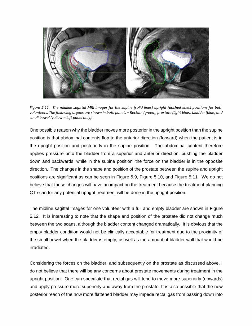
Figure 5.11. The midline sagittal MRI images for the supine (solid lines) upright (dashed lines) positions for both volunteers. The following organs are shown in both panels – Rectum (green), prostate (light blue), bladder (blue) and small bowel (yellow – left panel only).

One possible reason why the bladder moves more posterior in the upright position than the supine

position is that abdominal contents flop to the anterior direction (forward) when the patient is in

the upright position and posteriorly in the supine position. The abdominal content therefore

applies pressure onto the bladder from a superior and anterior direction, pushing the bladder

down and backwards, while in the supine position, the force on the bladder is in the opposite

direction. The changes in the shape and position of the prostate between the supine and upright

positions are significant as can be seen in Figure 5.9, Figure 5.10, and Figure 5.11. We do not

believe that these changes will have an impact on the treatment because the treatment planning

CT scan for any potential upright treatment will be done in the upright position.

The midline sagittal images for one volunteer with a full and empty bladder are shown in Figure

5.12. It is interesting to note that the shape and position of the prostate did not change much

between the two scans, although the bladder content changed dramatically. It is obvious that the

empty bladder condition would not be clinically acceptable for treatment due to the proximity of

the small bowel when the bladder is empty, as well as the amount of bladder wall that would be

irradiated.

Considering the forces on the bladder, and subsequently on the prostate as discussed above, I

do not believe that there will be any concerns about prostate movements during treatment in the

upright position. One can speculate that rectal gas will tend to move more superiorly (upwards)

and apply pressure more superiorly and away from the prostate. It is also possible that the new

posterior reach of the now more flattened bladder may impede rectal gas from passing down into

the actual rectal vault. If true, this could make treatment of the prostate gland more stable and

less susceptible to deformation due to the sudden dissention of rectal gas.

Figure 5.12. The midline sagittal MRI images for one of the volunteers with a full bladder (solid lines) and empty bladder (dashed lines) for the same volunteer in the upright position. The following organs are shown – Rectum (green), prostate (light blue), bladder (blue) and small bowel (yellow).

In summary, it appears that the position and shape of the bladder in the upright position might be

very favorable towards treating the prostate in the upright position. The risk of the small bowel

drooping into the posterior aspect of the treatment field might be reduced and looking at the

resultant pressure vectors on the bladder and prostate, it is quite possible that the prostate might

be better anchored in the upright position which would reduce unwanted movements and changes

in the prostate position and shape.

5.5. EFFICIENCIES IN PROTON THERAPY CLINICAL OPERATIONS

In 2010, I co-authored a chapter in a book edited by Dr. Ute Linz and titled, “Ion Beam Therapy

Fundamentals, Technology, Clinical Applications”. The title of our chapter is “Smaller – Lighter –

Cheaper: New Technological Concepts in Proton Therapy” [5.54]. This chapter discussed many

aspects of new and next generation proton therapy systems that would be required to make proton

therapy more viable and affordable. Over the years, Proton therapy vendors have implemented

many of the principles highlighted in that work. One of the aspects that was perhaps not

addressed extensively enough was general efficiencies in the day-to-day operation of a proton

clinic. Many institutions do not realize that inefficiencies are a recurring theme that will continue

to cost money.

The main reason, in my opinion, why operational efficiencies have not been addressed sufficiently

to date is the lack of volume in proton therapy systems. The initial expenses to establish a proton

therapy facility are much higher than a typical x-ray clinic but are a once off expense that are often

financed over an extended period. The day-to-day operations contribute to the annual operations

budget, which is often hard to meet, especially in the current weak medical coverage environment.

When we compare the current proton therapy operational aspects to the mainstream photon

therapy techniques, excluding the highly sophisticated special procedures, e.g. brachytherapy

and radiosurgery, we find that proton therapy systems typically require 2.5 to 3 times more

manpower and time. The time to construct a proton therapy system, from project inception to first

patient treatments, is also about 2.5 times longer. I have now doubt, as discussed earlier in this

chapter, that upright treatments will allow for reducing these ratios.

The first step in this pursuit is to reduce the cost of a proton therapy system. If upright treatments

are adopted into clinical practice the cost of a typical two room system will come down by at least

a factor of 2.5 since upright systems could be installed in existing cancer treatment facilities

obviating the need for new and expensive buildings. This will lead to many more proton therapy

facilities being build and many more people working on various aspects of proton therapy. This

will provide the financial resources and incentives to start implementing the prerequisites for

proton beam delivery discussed in this chapter. The benefits of implementing the listed

prerequisites on patient throughput and beam delivery efficiencies are numerous and have been

addressed in this chapter. One can argue that this is a chicken and egg situation, but I truly

believe there is enough momentum to push forward with upright treatments.

CHAPTER 6:

VALIDATING THE RAYSTATION MONTE CARLO DOSE

CALCULATION ALGORITHMS USING REALISTIC PHANTOMS.

6.1. OVERVIEW

This chapter will present two peer reviewed papers published in 2019 in the Journal of Applied

Clinical Medical Physics. The papers described the methods and experiments used to validate

the Monte Carlo dose calculation algorithms employed by the RayStation treatment planning

system for protons. The experiments employed various phantoms that I designed and developed

that mimicked near real life clinical situations. The fundamental physics behind these dose

calculation algorithms and the results of physical measurements to validate calculated dose

distributions in animal tissues and other phantoms is presented. This work required innovative

thinking in designing the phantoms and the measurements to realistically represent the real

clinical scenarios as possible.

The first peer reviewed paper describes the use of real animal tissue phantoms to validate the

Monte Carlo Dose calculation algorithms in static phantoms where motion and extreme tissue

inhomogeneities are not the main problem. The details of the first paper and the author list are

shown in figure 6.1. I initiated all the work described in this paper and developed all the phantoms,

the treatment plans and made the measurements in the proton beams. Dr. Ben Wilkinson is the

senior author since he was the medical director for the Provision Center for Proton Therapy in

Knoxville (PCPTK) where the work was done. Dr. Daniel Bridges was awarded second author

status since he was instrumental in getting the document into a shape to submit for publication.

Dr. Lauren Rigsby helped with the initial data analysis while she was doing her proton therapy

rotation at the Provision Center for Proton Therapy in Knoxville, TN (PCPTK) under the leadership

of Marc Blakey. Dr Martin Janson is a senior scientist at RaySearch, and he was instrumental in

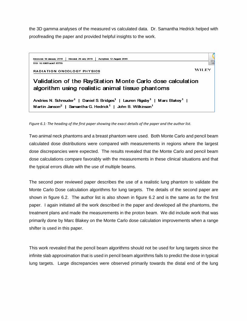
the 3D gamma analyses of the measured vs calculated data. Dr. Samantha Hedrick helped with

proofreading the paper and provided helpful insights to the work.

Figure 6.1: The heading of the first paper showing the exact details of the paper and the author list.

Two animal neck phantoms and a breast phantom were used. Both Monte Carlo and pencil beam

calculated dose distributions were compared with measurements in regions where the largest

dose discrepancies were expected. The results revealed that the Monte Carlo and pencil beam

dose calculations compare favorably with the measurements in these clinical situations and that

the typical errors dilute with the use of multiple beams.

The second peer reviewed paper describes the use of a realistic lung phantom to validate the

Monte Carlo Dose calculation algorithms for lung targets. The details of the second paper are

shown in figure 6.2. The author list is also shown in figure 6.2 and is the same as for the first

paper. I again initiated all the work described in the paper and developed all the phantoms, the

treatment plans and made the measurements in the proton beam. We did include work that was

primarily done by Marc Blakey on the Monte Carlo dose calculation improvements when a range

shifter is used in this paper.

This work revealed that the pencil beam algorithms should not be used for lung targets since the

infinite slab approximation that is used in pencil beam algorithms fails to predict the dose in typical

lung targets. Large discrepancies were observed primarily towards the distal end of the lung

target.

Figure 6.2: The heading of the second paper showing the exact details of the paper and the author list.

6.2. PEER REVIEWED PAPER 1 – MC VALIDATION FOR STATIC TARGETS.

TITLE: Validation of the RayStation Monte Carlo dose calculation algorithm using realistic animal tissue phantoms

6.2.1. INTRODUCTION

The growth in proton therapy facilities worldwide has accelerated greatly in recent years [6.1, 6.2],

mainly due to the clinical realization of pencil beam scanning (PBS) which increased the number

of applicable treatments [2.1]. Before the clinical utilization of PBS, proton therapy was limited to

small and contiguous targets because the beam had to be shaped by an aperture and distally

conformed to the target using a compensator. The increasing adoption of proton therapy is also

a result of reducing the costs and footprint of a typical facility. Recently, Bortfeld and Loeffler [6.3]

argued that changes in current health care policies would further drive this clinical implementation.

To accommodate this expansion, treatment planning systems had to improve and handle much

more complicated anatomical sites. Our institution chose the RayStation treatment planning

system (RaySearch Laboratories AB, Stockholm, Sweden) to handle this demand and was the

first proton therapy facility to use RayStation for proton therapy treatments [6.4, 6.5].

The first dose calculation models used for proton treatment planning employed raytracing

methods which only considered the deposition of dose along straight lines traced from the source

to the point of interest in the patient’s body. The deficiencies of these algorithms were well

understood, but they were the only option in the early days when computers were still very slow.

These algorithms were replaced by analytical pencil beam (APB) dose calculation algorithms as

described by Petti [2.23] and Hong [2.24]. The first releases of the RayStation treatment planning

system employed an APB algorithm for PBS that was partly based on the algorithm described by

Soukup and Fippel [2.25]. This APB dose engine divides the beam into many closely-spaced

mini-beams, called “pencil beams” [6.6]. Each pencil beam is calculated by factorization of the

lateral proton fluence and the integrated depth dose along the central axis of the pencil beam.

This factorization is only accurate given the infinite slab approximation in which the patient model

is composed of semi-infinite layers transverse to the central axis of the pencil beam. This

assumption is not satisfied in the presence of lateral heterogeneity, causing erroneous dose

calculation especially in lung targets. For the dose computation, the lateral proton fluence for each

pencil beam is affected by stopping power, Multiple Coulomb Scattering, and non-elastic nuclear

scattering. Summing all the individual pencil beams results in the total dose distribution [6.7].

RaySearch Laboratories AB released a Monte Carlo (MC) dose calculation engine in May 2017

(US release) to supplement and eventually replace the APB algorithm currently used in the

RayStation proton beam treatment planning system. In addition to improving the general

accuracies of the proton beam dose calculations within the patient, the three other major

improvements that the MC engine attempts are:

(1) accurate dose calculation for targets in lung and inhomogeneous mediums,

(2) accurate dose calculation when an aperture is used to sharpen the beam edge, and

(3) accurate shallow dose spots in the presence of a range shifter when large patient to

range shifter air gaps must be used.

The latter two issues are straightforward to address during validation using standard water

phantom measurements, but validating the dose in tissue, i.e. a realistic clinical situation, is much

harder.

This MC dose engine can be used for dose calculations for PBS and scattering-based treatment

deliveries. PBS deliveries allows for inverse treatment planning techniques where the weights of

a large number of candidate spots are determined using single-field optimization (SFO) or multi-

field optimization (MFO) strategies In RayStation, the Monte Carlo dose engine is not only used

for final dose computation of a given spot distribution, but may also be used in the optimization of

the plan. This means that the MC algorithm can be used to either calculate the final dose from

APB optimized spot distributions, or it can be used for optimization and final dose calculation. The

latter is the ideal option, but it can sometimes be time consuming especially during the initial

phases of the planning process. RaySearch Laboratories AB explains [6.7]:

The MC engine can account for range shifters and apertures with arbitrary air gaps. A Class

II transport algorithm is used for primary and secondary protons, while heavier secondary

particles such as deuterons and alphas are transported only by taking energy loss into

account using the Continuous Slowing Down Approximation (CSDA). [‘Class II’ methods

classify interactions into ‘hard’ and ‘soft’ categories depending on energy: Interactions

causing energy loss above a specified threshold (‘hard’ interactions) have their delta rays

explicitly modeled, whereas less-energetic interactions are summarized by sampling their

condensed history (a statistical summary of multiple interactions) [6.8] ] Neutral products such

as neutrons and Gammas are not transported, but their fractions of absorbed energy are

subtracted from the remaining beam. Delta electrons are considered to be stopped within 1

mm and are hence excluded from the beam’s calculation. The voxel grids of the simulation

geometry are “characterized by [each voxel having] its own mass density, elemental

composition, and mean ionization energy.” “Primary protons [are generated] in a plane

upstream of the patient transport grid [or] most upstream beam modifier,” and they are

transported “until they stop or [leave] the geometry. […] For increased performance, the

integration of the ionization energy loss is carried out by a parameterized model of the Bethe-

Bloc[h] equation. […] Energy loss straggling is [accounted for with] the Bohr approximation

[and] multiple scattering [uses] the theory of Goudsmit-Saunderson. Nonelastic reactions are

included by use of a data library of pre-stored tables of the needed quantities. The data library

is compiled from data provided in the ICRU Report 63 [6.9] for a sequence of elements in the

periodic table. The following quantities per element are used:

• total non-elastic cross section

• production cross section for proton, deuterons, and alpha particles

• fraction of incident energy leading to protons, deuterons, alphas, neutrals (neutrons and

gammas) and heavy recoils (A>4)

• double differential emission spectra for production of protons, deuterons, and alpha particles

When a new treatment modality such as PBS gains clinical utility, the question of treatment

planning accuracy must be addressed. The physics of therapeutic proton beam dose calculations

is generally less complicated than for x-rays and electrons since most of the energy deposition

mechanisms can be modelled by locally depositing the dose, at least within the voxel geometry

typically used for clinical dose calculations. This allows for MC dose calculation engines to be

simplified extensively, bringing down the computation times on standard computers to make

treatment planning feasible using less expensive computers. Many such models have been

developed over the years, [6.10, 6.11] but it was only recently that RayStation was equipped with

a clinical MC option [6.12]. Recent reports by Saini et. al. describe the process of commissioning

the RayStation planning system for clinical PBS treatments [6.13] and the dosimetric evaluation

of the RayStation MC algorithm [6.14] against phantom measurements and against the GATE

[6.15] MC dose engine. Recently Taylor et al [6.16] reported on the dose calculation inaccuracies

revealed by measurements using the IROC (Imaging and Radiation Oncology Core, Houston, TX,

USA) lung phantom. They found that when lung doses are calculated using APB, the target dose

was overestimated by 7 to 46%. Earlier this year, Widesott et al. validated this MC algorithm for

head-and-neck phantoms at multiple angles and air gaps at a single depth with a single gamma

analysis criteria [6.17]. The need to validate and transition to RayStation’s MC dose algorithm is

therefore clear.

Here we report on the more sophisticated clinical commissioning of the RayStation MC engine

employing clinically realistic scenarios and accurate dose measurements in various

anthropomorphic phantoms at multiple depths. We embarked on a series of experiments to

validate the MC doses versus doses measured in the near-reality phantoms for different

geometries. Using animal tissues to validate dose calculations is a common method and yielded

great results as described by Zheng [6.18], Grassberger [6.19], and Gurjar [6.20], though most of

this work was done for passively scattered or uniformly scanned proton beams. Our aim was to

develop phantoms that can validate the calculated dose “inside” the phantom and not “on the

other side”, i.e. a transmission-type measurement. In addition to this study, we also verified the

accuracy of MC calculations for lung; these findings are being prepared for subsequent

publication.

We note that similar work has recently been published regarding the open-source fast MC proton

dose algorithm MCsquare [6.21, 6.22], In a recent experimental study involving a measured

lateral profile measured in a water tank hosting a large lateral inhomogeneity, MCsquare was

compared to an early research version of the RaySearch MC algorithm. It was found that both

algorithms fared well in the study, but that RaySearch’s MC had a 2.5% better passing rate for a

2%/2mm gamma criterion [6.23]. With this experiment, we sought to build on this confidence of

the reliability of this dose algorithm. Specifically, for the safety and improvement of our clinical

practice we sought to answer the questions, “Does the current RayStation MC algorithm

accurately predict the dose to breast and head-and-neck sites?” and, “What is the magnitude of

improvement that MC provides over APB for dose distribution and range accuracy in breast and

head-and-neck sites?”

6.2.2. METHODS

6.2.2.1. Dose Validation Phantoms

Beams were delivered using the IBA Universal Nozzle in a gantry treatment room at a proton

center. The beams were delivered to the phantoms in a clinical setting, set up in the same manner

that a patient is positioned for treatment. The lamb neck and breast phantoms are shown in figure

6.3. The deer neck was similar in appearance and treated in the same manner.

Head and Neck (H&N) phantom

A lamb neck (figure 6.3) and a deer neck were used for the head-and-neck (H&N) phantoms. The

necks were cut while frozen with a radial saw to have a flat surface just past the neck vertebrae.

Both necks were then thawed and placed with their flat surfaces on 2 mm water-equivalent thick

solid water slabs, which in turn were placed on the MatriXX PT (Ion Beam Applications S.A.,

Louvain-la-Neuve, Belgium) detector to measure the dose distal but in close proximity to the neck

vertebrae. More solid water slabs were inserted between the phantom and the MatriXX PT to

make measurements at deeper depths beyond the neck solid water interface for each phantom.

Breast phantom

The breast phantom (figure 6.3) was a water-filled Mentor M+ 350 cc sample prothesis (Mentor

Worldwide LLC) [6.24] placed on solid water slabs of different thicknesses.

Figure 6.3. Representative phantoms used in this study: Lamb neck (left) and the water-filled Mentor M+ 350cc sample prothesis (right) as seen by photography (upper) and computed tomography (lower). The green box in the left bottom pane and the red line in the lower-right pane demarcates the dose optimization targets

6.2.2.2. Treatment planning

CT SIM

The dose validation phantoms were scanned as real patients with computed tomography (CT)

using a Siemens Somatom Definition AS CT scanner (Siemens Medical Solutions USA, Inc.,

Malvern, PA, USA). Care was taken to mark the phantoms for precise treatment planning and

positioning in the proton beam. The dose grid resolution was set to 1 mm for all final dose

computations, and the MC dose was computed to reach an average statistical uncertainty better

than 0.5% for voxels with a dose higher than 50% of the maximum dose. The dose computation

times required to calculate the final dose for each beam in this study using the MC and APB

algorithms are listed in Table 6.1.

Table 6.1. Dose calculation times compared for the MC and APB dose algorithms using uniform dose calculation grids of 1 mm and 2 mm, i.e. 1 mm3 and 8 mm3 voxels respectively.

Plan Grid Size Field Calculation Time (Sec) Ratio

tAPB tMC

(mm) (tMC/tAPB)

Deer Neck 1 F1 20 209 10.5

2 F1 7.3 35 4.8

1 F2 16.6 168 10.1

2 F2 7.4 30.8 4.2

Lamb Neck 1 F3 20.3 253 12.5

2 F3 5.7 42.3 7.4

1 F4 17.9 219 12.2

2 F4 5.9 38.6 6.5

The computations were done on a computer equipped with an Intel® Xenon CPU E-5 v3 with a

2.3GHz dual processor. All the beams were optimized using the APB algorithm only since the

purpose of the study was to compare the same beams, i.e. identical spot distributions and spot

doses. Re-optimizing the beams with the MC algorithm would have resulted in slightly different

spot distributions and spot doses due to the subtle differences in the algorithms addressed in this

work.

Dosimetry

For the neck phantoms, the dose optimization targets were 1 x 5 x 7 cm3 volumes drawn in the

solid water slabs at a depth posterior to the phantom solid water interface (the green boxes shown

in figure 6.4). Two different AP beams, F1 and F3 for the lamb and deer neck phantoms

respectively, were planned to deliver a deliberately non-uniform dose distribution beyond the

animal tissue as shown in figure 6.4. We created plans using the APB algorithm for plan

optimization [6.25, 6.26]. The non-uniform dose distributions were accomplished by first overriding

the material in the red volumes shown in figure 6.4, panels A and B, to water and optimizing the

beam to deliver a uniform dose in the target (green boxes in Figure 6.4). Secondly, the material

override was then removed to recalculate the dose distributions resulting in a non-uniform

distribution due to the presence of the heterogeneities in the neck phantoms.

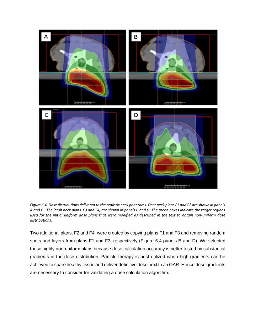
Figure 6.4. Dose distributions delivered to the realistic neck phantoms. Deer neck plans F1 and F2 are shown in panels A and B. The lamb neck plans, F3 and F4, are shown in panels C and D. The green boxes indicate the target regions used for the initial uniform dose plans that were modified as described in the text to obtain non-uniform dose distributions.

Two additional plans, F2 and F4, were created by copying plans F1 and F3 and removing random

spots and layers from plans F1 and F3, respectively (Figure 6.4 panels B and D). We selected

these highly non-uniform plans because dose calculation accuracy is better tested by substantial

gradients in the dose distribution. Particle therapy is best utilized when high gradients can be

achieved to spare healthy tissue and deliver definitive dose next to an OAR. Hence dose gradients

are necessary to consider for validating a dose calculation algorithm.

Figure 6.5. The breast phantom showing the beam orientations and measurement depths used. The red line demarcates the dose optimization target. The dose distributions shown were calculated with the APB algorithm.

The treatment plan for the breast phantom, shown in figure 6.5, followed a similar approach to

the neck phantoms except that we drew an irregular target volume crossing over into the solid

water to enable calculating and measuring dose beyond the breast prosthesis. We were primarily

interested in the dose adjacent to the patient’s breast tissue, i.e. the rib dose and at beam edges

where the breast tissue forms a significant roll or other discrete soft-tissue-to-air interface or

oblique interface to the beam. Dose was optimized for the red target volume shown in figure 6.3

(bottom right panel) and figure 6.5 considering en-face and oblique beams.

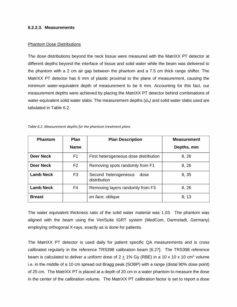
6.2.2.3. Measurements

Phantom Dose Distributions

The dose distributions beyond the neck tissue were measured with the MatriXX PT detector at

different depths beyond the interface of tissue and solid water while the beam was delivered to

the phantom with a 2 cm air gap between the phantom and a 7.5 cm thick range shifter. The

MatriXX PT detector has 6 mm of plastic proximal to the plane of measurement, causing the

minimum water-equivalent depth of measurement to be 6 mm. Accounting for this fact, our

measurement depths were achieved by placing the MatriXX PT detector behind combinations of

water-equivalent solid water slabs. The measurement depths (dm) and solid water slabs used are

tabulated in Table 6.2.

Table 6.2. Measurement depths for the phantom treatment plans

Phantom Plan

Name

Plan Description Measurement

Depths, mm

Deer Neck F1 First heterogeneous dose distribution 8, 26

Deer Neck F2 Removing spots randomly from F1 8, 26

Lamb Neck F3 Second heterogeneous dose

distribution

8, 35

Lamb Neck F4 Removing layers randomly from F3 8, 26

Breast en face; oblique 8, 13

The water equivalent thickness ratio of the solid water material was 1.03. The phantom was

aligned with the beam using the VeriSuite IGRT system (MedCom, Darmstadt, Germany)

employing orthogonal X-rays, exactly as is done for patients.

The MatriXX PT detector is used daily for patient specific QA measurements and is cross

calibrated regularly in the reference TRS398 calibration beam [6.27]. The TRS398 reference

beam is calculated to deliver a uniform dose of 2 + 1% Gy (RBE) in a 10 x 10 x 10 cm3 volume

i.e. in the middle of a 10 cm spread out Bragg peak (SOBP) with a range (distal 90% dose point)

of 25 cm. The MatriXX PT is placed at a depth of 20 cm in a water phantom to measure the dose

in the center of the calibration volume. The MatriXX PT calibration factor is set to report a dose

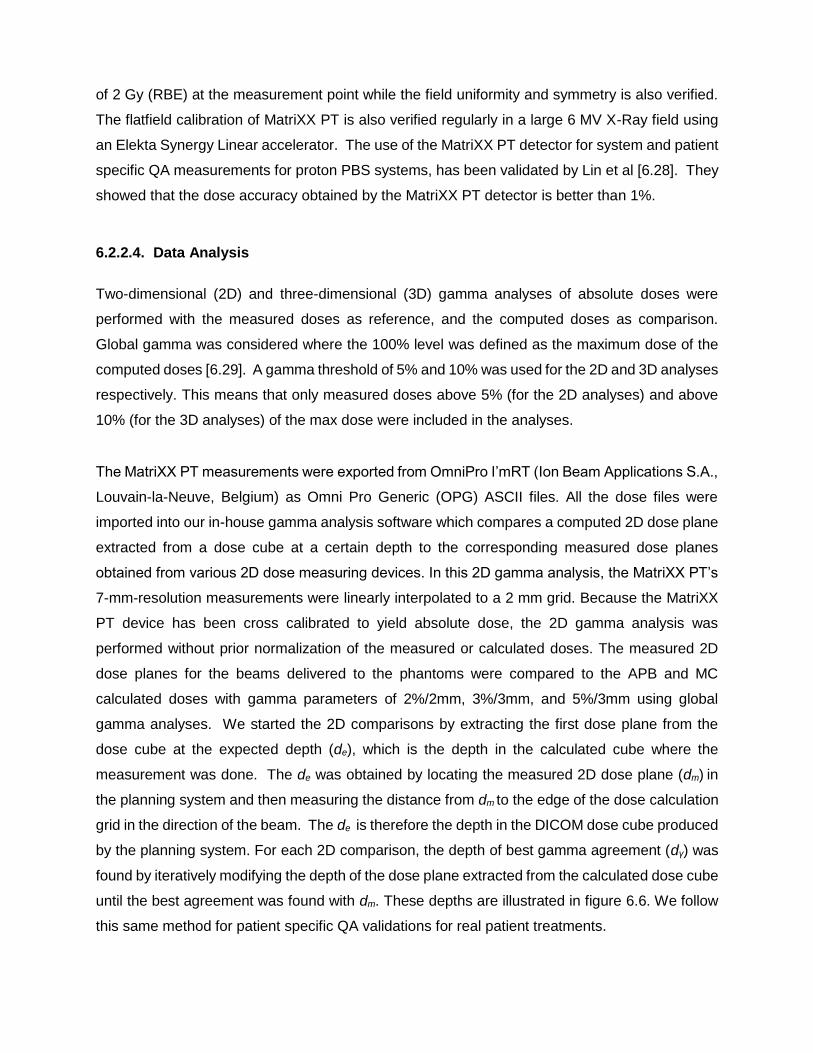
of 2 Gy (RBE) at the measurement point while the field uniformity and symmetry is also verified.

The flatfield calibration of MatriXX PT is also verified regularly in a large 6 MV X-Ray field using

an Elekta Synergy Linear accelerator. The use of the MatriXX PT detector for system and patient

specific QA measurements for proton PBS systems, has been validated by Lin et al [6.28]. They

showed that the dose accuracy obtained by the MatriXX PT detector is better than 1%.

6.2.2.4. Data Analysis

Two-dimensional (2D) and three-dimensional (3D) gamma analyses of absolute doses were

performed with the measured doses as reference, and the computed doses as comparison.

Global gamma was considered where the 100% level was defined as the maximum dose of the

computed doses [6.29]. A gamma threshold of 5% and 10% was used for the 2D and 3D analyses

respectively. This means that only measured doses above 5% (for the 2D analyses) and above

10% (for the 3D analyses) of the max dose were included in the analyses.

The MatriXX PT measurements were exported from OmniPro I’mRT (Ion Beam Applications S.A.,

Louvain-la-Neuve, Belgium) as Omni Pro Generic (OPG) ASCII files. All the dose files were

imported into our in-house gamma analysis software which compares a computed 2D dose plane

extracted from a dose cube at a certain depth to the corresponding measured dose planes

obtained from various 2D dose measuring devices. In this 2D gamma analysis, the MatriXX PT’s

7-mm-resolution measurements were linearly interpolated to a 2 mm grid. Because the MatriXX

PT device has been cross calibrated to yield absolute dose, the 2D gamma analysis was

performed without prior normalization of the measured or calculated doses. The measured 2D

dose planes for the beams delivered to the phantoms were compared to the APB and MC

calculated doses with gamma parameters of 2%/2mm, 3%/3mm, and 5%/3mm using global

gamma analyses. We started the 2D comparisons by extracting the first dose plane from the

dose cube at the expected depth (de), which is the depth in the calculated cube where the

measurement was done. The de was obtained by locating the measured 2D dose plane (dm) in

the planning system and then measuring the distance from dm to the edge of the dose calculation

grid in the direction of the beam. The de is therefore the depth in the DICOM dose cube produced

by the planning system. For each 2D comparison, the depth of best gamma agreement (dγ) was

found by iteratively modifying the depth of the dose plane extracted from the calculated dose cube

until the best agreement was found with dm. These depths are illustrated in figure 6.6. We follow

this same method for patient specific QA validations for real patient treatments.

Figure 6.6. A schematic showing the "expected DICOM depth" de, i.e. the depth in the DICOM dose file at which we expect the best gamma index agreement given accurate dose calculation; the depth of measurement dm; and the depth of best gamma index agreement dγ. de is measured from the anterior surface of the dose cube (dotted line) to the placement of the measuring plane inside the MatriXX PT (blue dashed line). dm is measured from the solid-water surface (blue line) to the same position. dγ is determined by varying the dose calculation plane until best agreement is obtained with our in-house software given the reference position of solid water surface (blue line).

We also performed 3D gamma analyses of all the MatriXX PT measured data using tools in the

RaySearch Laboratories dose engine validation test suite. The 3D gamma analyses were

performed between the measured dose plane and the calculated dose plane extracted at the

expected depth (de). The gamma analysis tools in this internal software package are the same

as those included in the clinically available product Compass from IBA Dosimetry and RaySearch

[6.30]. In this gamma analysis, the sparsely measured data points were used as the reference

dose with the computed 3D dose as evaluation, which is the converse of the 2D gamma analyses

described above.

Table 6.3. Gamma analysis results for the animal tissue neck phantoms. The comparative data for the animal tissue phantoms from the RaySearch team is included. Depth difference to best gamma agreement for the 2D analyses is listed in the column labelled de - dγ .

6.2.2.5. Results

Dose calculation times

The dose calculation times required by the MC algorithm (tMC) are significantly longer than for

APB algorithm (tAPB) and scales approximately as the inverse cube of the dose computation grid

size. The ratio of tMC/tAPB is also listed in Table 6.1 showing that the MC calculation times are on

average 5.7 +1.5 (1 Stdev) and 11.3 + 1.2 (1 Stdev) times longer for beams using 2 and 1 mm

grid spacings respectively . It is expected that tMC will be reduced significantly when GPU based

calculations become available in future releases of the RayStation software.

Gamma Analyses

The gamma passing rates for the animal neck phantoms and breast phantom are listed in tables

3 and 4. The depths of best 2D gamma agreement for the neck phantoms are also listed in Table

6.3. We report the 3D gamma pass rates at the expected measurement planes.

Neck Phantoms

Calculated dose distributions for the F3 lamb neck plan are shown in figure 6.7 for the axial slice

where the largest disagreements were observed. MC-calculated dose was about 20% less than

APB-calculated dose in some areas due to the bone tissue interfaces. The upper left panel shows

the MC dose while the bottom left panel shows the APB dose. The line profiles shown in the right

panel were extracted along the solid straight lines shown in the left panels. The APB algorithm

has problems in the vicinity of extreme density variations caused by the air-bone interface (figure

6.7). It is important to notice that the depth doses shown by the blue lines in the right panel of

figure 6.7 are not dramatically affected by the heterogeneity. Lateral dose profiles calculated with

MC and APB for the F3 lamb neck plan at a depth of 35 mm in solid water corresponding to the

expected DICOM depth of 101.3 mm are compared with the corresponding measured profile in

figure 6.8. Screenshots from our in-house 2D gamma analysis software are shown in figure 6.9

and Figure 6.10 for the F3 plan of the lamb neck phantom at the two measurement depths of 8

mm (expected DICOM depth = 74.1 mm) and 35 mm (expected DICOM depth = 101.3 mm) in

solid water. The bottom right panels in figure 6.9 and figure 6.10 show the gamma analyses

panes.

Figure 6.7. A comparison of dose distributions calculated by the Monte Carlo algorithm (upper left) and analytical pencil beam algorithm (lower left) for the lamb neck phantom in the region where the largest differences were observed. The depth dose and lateral dose profiles along the vertical pale blue and horizontal green lines in the left panels are shown in the right pane for the MC (solid) and APB (dotted) doses

Figure 6.8. Lateral profiles comparing the MatriXX PT measured (blue triangles), MC calculated (red lines), and APB calculated (green lines) at a measurement depth of 35 mm in solid water (Dicom depth = 101.3 mm) for the lamb neck phantom plan F3.

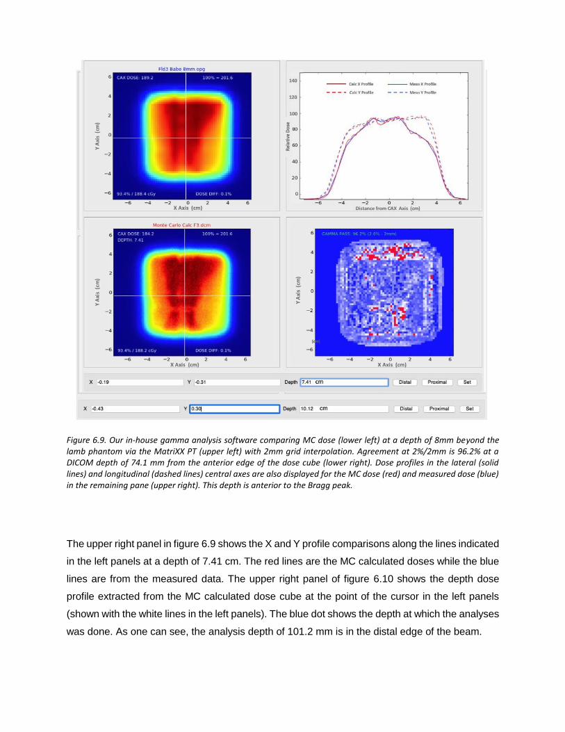
Figure 6.9. Our in-house gamma analysis software comparing MC dose (lower left) at a depth of 8mm beyond the lamb phantom via the MatriXX PT (upper left) with 2mm grid interpolation. Agreement at 2%/2mm is 96.2% at a DICOM depth of 74.1 mm from the anterior edge of the dose cube (lower right). Dose profiles in the lateral (solid lines) and longitudinal (dashed lines) central axes are also displayed for the MC dose (red) and measured dose (blue) in the remaining pane (upper right). This depth is anterior to the Bragg peak.

The upper right panel in figure 6.9 shows the X and Y profile comparisons along the lines indicated

in the left panels at a depth of 7.41 cm. The red lines are the MC calculated doses while the blue

lines are from the measured data. The upper right panel of figure 6.10 shows the depth dose

profile extracted from the MC calculated dose cube at the point of the cursor in the left panels

(shown with the white lines in the left panels). The blue dot shows the depth at which the analyses

was done. As one can see, the analysis depth of 101.2 mm is in the distal edge of the beam.

Figure 6.10. Our in-house gamma analysis software comparing MC dose (lower left) at a depth of 35mm beyond the lamb phantom (see figure 6.4) via the MatriXX PT (upper left) with 2mm grid interpolation. Agreement at 3%/3mm is 96.2% at a DICOM depth of 101.2 mm from the anterior edge of the dose cube (lower right). This depth is within the Bragg peak falloff (upper right).

Breast Phantom

For the breast plans, only 3D gamma analysis was performed. The passing rates are listed in

Table 6.4.

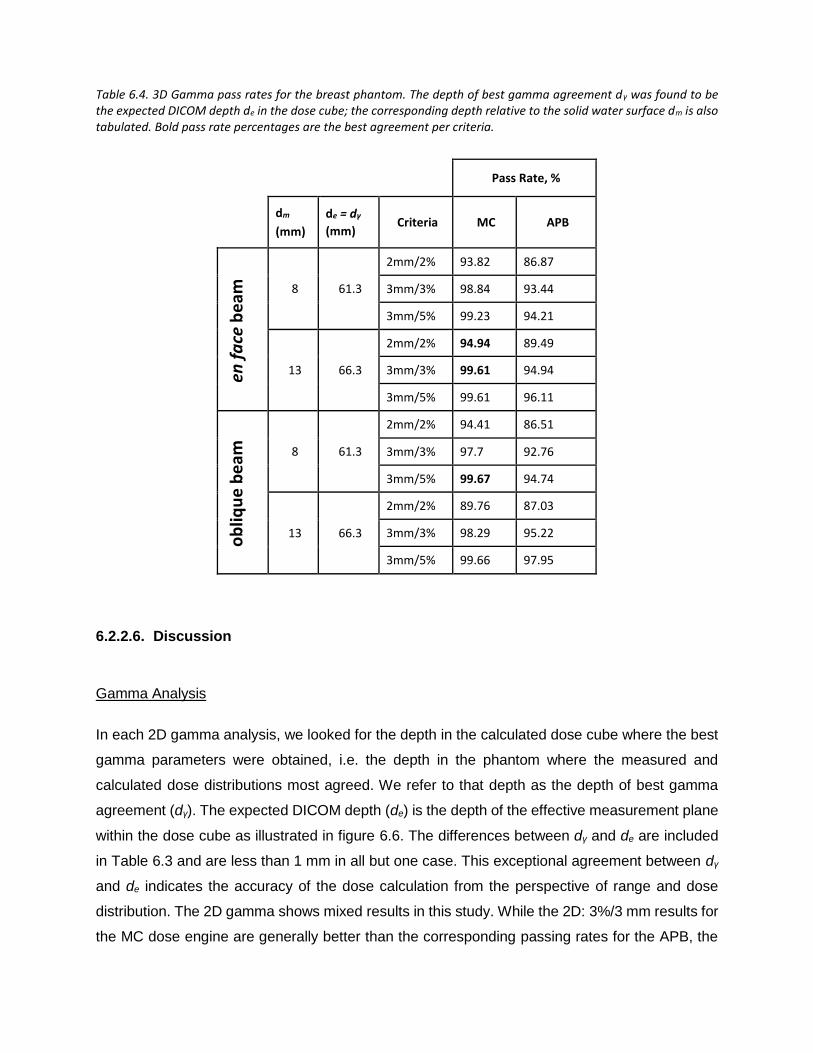
Table 6.4. 3D Gamma pass rates for the breast phantom. The depth of best gamma agreement dγ was found to be the expected DICOM depth de in the dose cube; the corresponding depth relative to the solid water surface dm is also tabulated. Bold pass rate percentages are the best agreement per criteria.

Pass Rate, %

dm

(mm)

de = dγ

(mm) Criteria MC APB

8 61.3

2mm/2% 93.82 86.87

3mm/3% 98.84 93.44

3mm/5% 99.23 94.21

13 66.3

2mm/2% 94.94 89.49

3mm/3% 99.61 94.94

3mm/5% 99.61 96.11

8 61.3

2mm/2% 94.41 86.51

3mm/3% 97.7 92.76

3mm/5% 99.67 94.74

13 66.3

2mm/2% 89.76 87.03

3mm/3% 98.29 95.22

3mm/5% 99.66 97.95

6.2.2.6. Discussion

Gamma Analysis

In each 2D gamma analysis, we looked for the depth in the calculated dose cube where the best

gamma parameters were obtained, i.e. the depth in the phantom where the measured and

calculated dose distributions most agreed. We refer to that depth as the depth of best gamma

agreement (dγ). The expected DICOM depth (de) is the depth of the effective measurement plane

within the dose cube as illustrated in figure 6.6. The differences between dγ and de are included

in Table 6.3 and are less than 1 mm in all but one case. This exceptional agreement between dγ

and de indicates the accuracy of the dose calculation from the perspective of range and dose

distribution. The 2D gamma shows mixed results in this study. While the 2D: 3%/3 mm results for

the MC dose engine are generally better than the corresponding passing rates for the APB, the

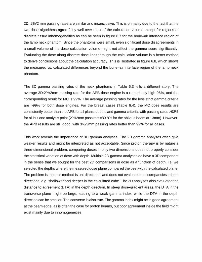
2D: 2%/2 mm passing rates are similar and inconclusive. This is primarily due to the fact that the

two dose algorithms agree fairly well over most of the calculation volume except for regions of

discrete tissue inhomogeneities as can be seen in figure 6.7 for the bone–air interface region of

the lamb neck phantom. Since the phantoms were small, even significant dose disagreements in

a small volume of the dose calculation volume might not affect the gamma score significantly.

Evaluating the dose along discrete dose lines through the calculation volume is a better method

to derive conclusions about the calculation accuracy. This is illustrated in figure 6.8, which shows

the measured vs. calculated differences beyond the bone–air interface region of the lamb neck

phantom.

The 3D gamma passing rates of the neck phantoms in Table 6.3 tells a different story. The

average 3D:2%/2mm passing rate for the APB dose engine is a remarkably high 96%, and the

corresponding result for MC is 99%. The average passing rates for the less strict gamma criteria

are >99% for both dose engines. For the breast cases (Table 6.4), the MC dose results are

consistently better than the APB for all plans, depths and gamma criteria, with passing rates >93%

for all but one analysis point (2%/2mm pass rate=89.8% for the oblique beam at 13mm). However,

the APB results are still good, with 3%/3mm passing rates better than 92% for all cases.

This work reveals the importance of 3D gamma analyses. The 2D gamma analyses often give

weaker results and might be interpreted as not acceptable. Since proton therapy is by nature a

three-dimensional problem, comparing doses in only two dimensions does not properly consider

the statistical variation of dose with depth. Multiple 2D gamma analyses do have a 3D component

in the sense that we sought for the best 2D comparisons in dose as a function of depth, i.e. we

selected the depths where the measured dose plane compared the best with the calculated plane.

The problem is that this method is uni-directional and does not evaluate the discrepancies in both

directions, e.g. shallower and deeper in the calculated cube. The 3D analyses also evaluated the

distance to agreement (DTA) in the depth direction. In steep dose-gradient areas, the DTA in the

transverse plane might be large, leading to a weak gamma index, while the DTA in the depth

direction can be smaller. The converse is also true. The gamma index might be in good agreement

at the beam edge, as is often the case for proton beams, but poor agreement inside the field might

exist mainly due to inhomogeneities.

Benefits of the Monte Carlo dose calculations

The data shown in this report validates the use of the MC dose calculation engine in RayStation

for clinical use. The main benefits of a MC dose engine are for dose calculations in lung and for

beams where a range shifter and larger airgap is required. We investigated these as well and the

work will be presented in a subsequent study. In this study, the airgap was kept rather small and

the lateral inhomogeneities of the phantoms were limited. Consequently, the accuracy of the APB

dose algorithm was found to be acceptable (in terms of passing rates of 3%/3 mm gamma

analysis), although the MC dose accuracy was consistently better. The differences in the dose

calculations from the APB and MC dose engines are very similar for the most part. Significant

differences in dose ( > 24%) occur after the beam traverses discrete density changes as seen in

figure 6.7 and figure 6.8. It is important to note that the largest differences are observed for single

beams in the head-and-neck region, however single beams are not often used in the clinical

setting. These kinds of interface errors are diminished by using multiple beams traversing the

interface at different angles.

We note also the overall difference in dose conformality. MC calculations are more granular

whereas the APB calculations appear smoother. This is because the APB algorithm is using the

infinite slab approximation as described earlier, which is clearly not addressing the density

interfaces correctly. This is most likely the primary reason why the MC calculations struggle to

demonstrate superiority over APB calculations at the stricter gamma criteria and more so for the

2D analyses. In areas where there are no discrete density changes, the calculations agree very

well.

6.2.2.7. Conclusions

In this work we validated the RayStation 6 Monte Carlo and APB dose calculation algorithms for

head-and-neck and breast phantoms. The MC results were systematically better than the APB

results, although APB was found to be clinically acceptable for the studied cases. We further

demonstrated depth-dose discrepancy to be less than 1% for both algorithms. This work also

highlighted the spatial limitation of 2D gamma, supporting the use of 3D gamma analyses for

evaluating 3D dose distributions. Similar to isodose curves complementing dose-volume

histograms, we must pay attention to where the gamma-index criteria are not satisfied in addition

to the relative percentage to which it is satisfied.

We recommend implementing the RayStation Monte Carlo algorithm as a direct means to improve

accuracy in treatment planning. Our future work will discuss the influence of air gap, range

shifters, and apertures on this algorithm’s accuracy. We will also validate this algorithm for targets

in lung tissue using a novel phantom allowing dose measurement within a realistic tumor

phantom.

6.3. PEER REVIEWED PAPER 2 – MC VALIDATION FOR LUNG

TARGETS.

TITLE: Validation of the RayStation Monte Carlo dose calculation algorithm using a realistic lung phantom

6.3.1. Introduction

Lung and bronchus is now the most common cancer site in sixteen states and second overall in

the United States, with only 12% fewer estimated cases than female breast [6.31]. Given the

principle to keep radiation exposure as low as reasonably achievable [6.32], combined with the

benefits of hypo fractionated proton therapy [6.33-6.36], the need to increase the accuracy of

proton radiotherapy to thoracic sites has thus become imperative. Most proton clinics are currently

using commercially available analytical pencil beam (APB) algorithms [2.24, 6.37, 6.38]. These

APB algorithms are typically designed to be computationally efficient, but inherently include

simplifications of the transport problem as compared to e.g. Monte Carlo (MC) based algorithms.

Consequently, the APB algorithm sometimes suffers loss of accuracy in areas of inhomogeneity,

such as in lung, where even small algorithmic deficiencies can result in significant shifts of dose

distributions [6.11]. It has been shown by Taylor et al. that the APB algorithm is “doing a poor

job” of predicting dose in lung tumors, with over-predictions up to 46% in the PTV [6.16]. In the

case of lateral heterogeneities, MC dose calculation algorithms are superior in calculating

accurate dose distributions [2.39,6.40]. MC is viewed as the gold standard for dose calculation

for most radiation transport calculations, but traditional MC algorithms such as MCNPX [6.41] and

Geant4 [6.42] are too slow to keep up with clinical workflow. To combat this problem, Fast Monte

Carlo (FMC) dose engines have been developed for clinical use [6.10, 6.11]. A study by Sorriaux

et al. compared both MC and FMC dose engines with APB in clinical situations of heterogeneity.

They found that FMC corresponded well with data measured in an inhomogeneous phantom

made of water surrounding a long insert of bone tissue substitute, whereas more than half of the

APB dose distributions failed gamma-index analysis [6.23].

We explain in another study how the RaySearch APB and MC algorithms work [6.43]. When the

MC dose engine became available in RayStation 6 (RaySearch Laboratories AB, Stockholm,

Sweden), we proposed to validate it using animal tissue and realistic phantoms, because the use

of animal tissue phantoms in dose validation has seen useful results,[6.15] [6.16 similar to using

wood or cork to approximate lung tissue [6.17] [6.18] [6.44]. Previously, we studied these

algorithms applied to animal neck phantoms and a water-based breast phantom [2.40]. In this

study, we focused on validating the MC algorithm for a more complex lung phantom made of a

composite of lamb ribs, ground lamb meat and cork. We demonstrate that we can measure dose

inside a realistic lung tumor phantom for a target not adjacent to the chest wall, i.e. a tumor

surrounded by lower density lung tissue. We then compared the measured data with doses

calculated using the RaySearch APB and MC algorithms. We searched articles available to the

public from multiple journals concerning lung phantoms. Although a number of phantoms have

been tested, including solid water [6.45, 6.46] cork and solid water [6.47-6.50], balsa wood and

solid water [6.51], balsa wood and cork [6.16], cork and plastic [6.52, 6.53], cork and acrylic [6.54,

6.55], polystyrene and cork [6.56], bolus and sponge [6.57], foam [6.58, 6.59], and even wood

[6.60, 6.61], it appears that we are the first to report open-access on the use of a cork-and-animal

tissue lung tumor phantom.

6.3.2. Methods Dose Validation Phantom

The lung phantom is shown in Figure 6.11. The lung phantom was composed of a rack of lamb

containing real rib bones, intercostal muscle, and fat. To simulate lung tissue beneath the lamb

rack, we placed 5.0 + 0.5 mm thick layers of Quartet cork (ACCO Brands, Lake Zurich, Illinois;

SKU 48112Q) obtained from a hardware store. The cork slabs and the rack of lamb were pinned

together using wooden toothpicks to allow for splitting and re-assembling the phantom accurately

enabling measurements “inside” the phantom.

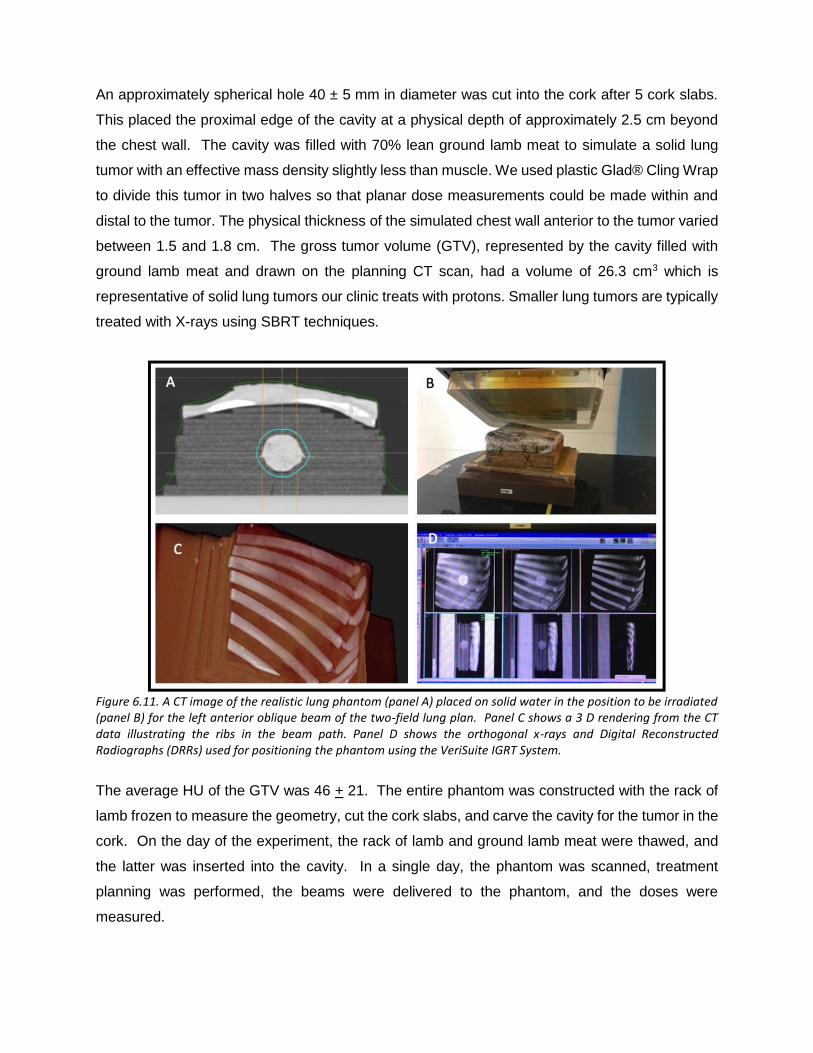
An approximately spherical hole 40 ± 5 mm in diameter was cut into the cork after 5 cork slabs.

This placed the proximal edge of the cavity at a physical depth of approximately 2.5 cm beyond

the chest wall. The cavity was filled with 70% lean ground lamb meat to simulate a solid lung

tumor with an effective mass density slightly less than muscle. We used plastic Glad® Cling Wrap

to divide this tumor in two halves so that planar dose measurements could be made within and

distal to the tumor. The physical thickness of the simulated chest wall anterior to the tumor varied

between 1.5 and 1.8 cm. The gross tumor volume (GTV), represented by the cavity filled with

ground lamb meat and drawn on the planning CT scan, had a volume of 26.3 cm3 which is

representative of solid lung tumors our clinic treats with protons. Smaller lung tumors are typically

treated with X-rays using SBRT techniques.

Figure 6.11. A CT image of the realistic lung phantom (panel A) placed on solid water in the position to be irradiated (panel B) for the left anterior oblique beam of the two-field lung plan. Panel C shows a 3 D rendering from the CT data illustrating the ribs in the beam path. Panel D shows the orthogonal x-rays and Digital Reconstructed Radiographs (DRRs) used for positioning the phantom using the VeriSuite IGRT System.

The average HU of the GTV was 46 + 21. The entire phantom was constructed with the rack of

lamb frozen to measure the geometry, cut the cork slabs, and carve the cavity for the tumor in the

cork. On the day of the experiment, the rack of lamb and ground lamb meat were thawed, and

the latter was inserted into the cavity. In a single day, the phantom was scanned, treatment

planning was performed, the beams were delivered to the phantom, and the doses were

measured.

6.3.3. Treatment Planning

The lung phantom was scanned on a Siemens Somatom Definition AS CT scanner (Siemens

Medical Solutions USA, Inc., Malvern, PA, USA) using a 50 cm Field of View (FOV) obtaining 512

x 512 pixel axial images (0.98 x 0.98 mm2 pixel size) reconstructed with a 4 mm slice distance

between images (131 axial images) . The phantom was marked with a pen and BBs to ensure

the alignment could be accurately reproduced. Using RayStation, the GTV was delineated and

expanded to a CTV using a 5 mm uniform margin.

Figure 6.12. Dose distributions for the two lung phantom plans shown in the axial CT slices through the isocenter. The 1 Field lung phantom plan dose distribution calculated with APB is shown in panel A and the corresponding MC dose distribution is shown in panel C. The 2 Field lung phantom plan dose distribution calculated with APB is shown in panel B and the corresponding MC dose distribution is shown in panel D.

The CTV was used as the target in the optimization of the plans. We developed two pencil-beam

scanning (PBS) plans as shown in Figure 6.12. The first plan used a single anterior field and a

second plan used two anterior oblique fields that were optimized using the single field uniform

dose (SFUD) technique i.e. each field delivered a uniform dose to the CTV. For both plans, the

isocenter was centered within the tumor. A 7.5 cm WET Lucite range shifter with physical

thickness of 6.7 cm was used, and the airgap, here defined as the smallest distance between the

range shifter and the phantom surface, -was kept as small as possible. An air gap of 1.6 cm was

used for the single-field lung plan. Beam 1 of the two-field plan also used a 1.6 cm airgap while

beam 2 used a 2 cm airgap. The two plans were optimized to deliver a uniform dose of 2 Gy(RBE)

in one fraction to the target

The plans were optimized using the APB algorithm in RayStation (RS) 6.0 using a 1 x 1 x 1 mm3

calculation grid. The doses of the APB plans were then recomputed using the RS 6.0 MC dose

engine to a statistical uncertainty in the high dose region of 0.5% per beam. The RS6.0 APB

doses were subsequently recomputed using RS 6.2, due to an updated handling of the range

shifter in the APB algorithm that became available in that version.

Figure 6.13. A comparison between measured and calculated central axis (CAX) doses for a PBS beam for different air gaps between the range shifter and the water surface. The measured data points are indicated by the red squares while the MC data and the APB calculated doses are shown by the green and blue lines respectively. The extent of the airgap for each graph is printed as the title of each panel.

One of the known deficiencies of the APB algorithm is calculating the dose when a range shifter

is used [6.62]. During commissioning of the APB RS 6.2 and the MC RS 6.0 algorithms for clinical

use, we measured the CAX depth dose for a typical breast treatment beam with a Markus parallel

plate ionization chamber in a water tank for a zero-degree gantry angle. We used different air

gaps between the range shifter and the water surface. The deficiencies in APB calculations were

confirmed as can be seen in Figure 6.13. It is clear from the data in Figure 6.13 that the MC

algorithm reduces the uncertainty with airgap to a clinically insignificant level. To minimize this

airgap effect of the APB dose engine, we kept the airgaps as small as possible in this study.

Figure 6.14. Measurement depths illustrated for verifying the calculated dose for the Anterior 1 field plan. The MatriXX PT rectangular slab contours for the mid and the distal measurement planes are illustrated with the teal and violet contours respectively. The dark blue rectangular contour shows the volume used to calculate the HU histogram shown in Figure 6.15.

The MatriXX PT detector (Ion Beam Applications S.A., Louvain-la-Neuve, Belgium) used to

measure the dose in the lung phantom has a 6.2 mm water-equivalent buildup region proximal to

the plane of measurement. This build-up region was included in our treatment plans by drawing

two 6.2 x 80 mm2 rectangular slab contours on each axial CT slice within the treatment volume.

The top edge of each contour was aligned with the mid and distal measurement planes,

respectively, i.e. the positions in the phantom where the proximal surface of the MatriXX PT

detector was located during the respective measurements. We simulated the insertion of the

MatriXX PT detector by overriding the material in the 6.2 mm rectangular slab contours, referred

to hereafter as “the MatriXX PT slab”, to water. The dose was recalculated for each of the

measurement conditions at the mid and distal planes. When the mid plane dose was calculated,

the MatriXX PT slab in the middle of the tumor was set to water, while the material for the distal

MatriXX PT slab was not overridden. The opposite was true for when distal plane dose was

calculated. The mid plane MatriXX PT slab contour (teal contour) and the distal plane MatriXX

PT slab contour (purple contour) are shown in Figure 6.14

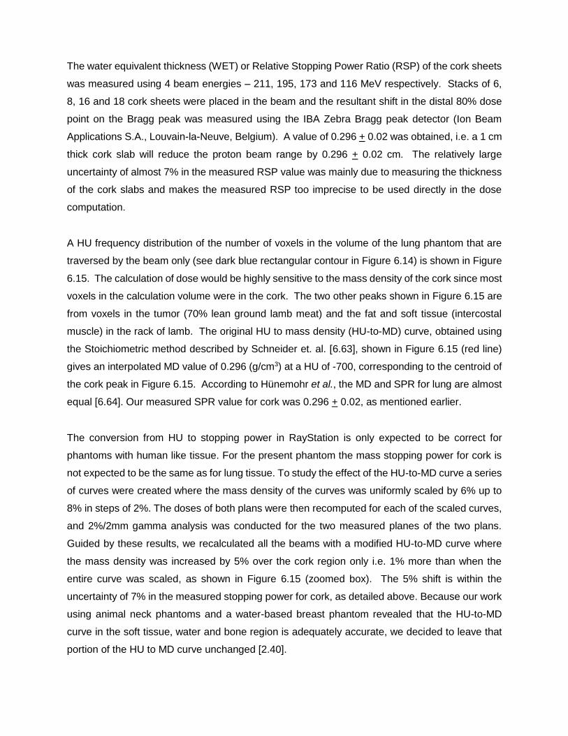
The water equivalent thickness (WET) or Relative Stopping Power Ratio (RSP) of the cork sheets

was measured using 4 beam energies – 211, 195, 173 and 116 MeV respectively. Stacks of 6,

8, 16 and 18 cork sheets were placed in the beam and the resultant shift in the distal 80% dose

point on the Bragg peak was measured using the IBA Zebra Bragg peak detector (Ion Beam

Applications S.A., Louvain-la-Neuve, Belgium). A value of 0.296 + 0.02 was obtained, i.e. a 1 cm

thick cork slab will reduce the proton beam range by 0.296 + 0.02 cm. The relatively large

uncertainty of almost 7% in the measured RSP value was mainly due to measuring the thickness

of the cork slabs and makes the measured RSP too imprecise to be used directly in the dose

computation.

A HU frequency distribution of the number of voxels in the volume of the lung phantom that are

traversed by the beam only (see dark blue rectangular contour in Figure 6.14) is shown in Figure

6.15. The calculation of dose would be highly sensitive to the mass density of the cork since most

voxels in the calculation volume were in the cork. The two other peaks shown in Figure 6.15 are

from voxels in the tumor (70% lean ground lamb meat) and the fat and soft tissue (intercostal

muscle) in the rack of lamb. The original HU to mass density (HU-to-MD) curve, obtained using

the Stoichiometric method described by Schneider et. al. [6.63], shown in Figure 6.15 (red line)

gives an interpolated MD value of 0.296 (g/cm3) at a HU of -700, corresponding to the centroid of

the cork peak in Figure 6.15. According to Hünemohr et al., the MD and SPR for lung are almost

equal [6.64]. Our measured SPR value for cork was 0.296 + 0.02, as mentioned earlier.

The conversion from HU to stopping power in RayStation is only expected to be correct for

phantoms with human like tissue. For the present phantom the mass stopping power for cork is

not expected to be the same as for lung tissue. To study the effect of the HU-to-MD curve a series

of curves were created where the mass density of the curves was uniformly scaled by 6% up to

8% in steps of 2%. The doses of both plans were then recomputed for each of the scaled curves,

and 2%/2mm gamma analysis was conducted for the two measured planes of the two plans.

Guided by these results, we recalculated all the beams with a modified HU-to-MD curve where

the mass density was increased by 5% over the cork region only i.e. 1% more than when the

entire curve was scaled, as shown in Figure 6.15 (zoomed box). The 5% shift is within the

uncertainty of 7% in the measured stopping power for cork, as detailed above. Because our work

using animal neck phantoms and a water-based breast phantom revealed that the HU-to-MD

curve in the soft tissue, water and bone region is adequately accurate, we decided to leave that

portion of the HU to MD curve unchanged [2.40].

Figure 6.15. The frequency distribution of the number of voxels vs. Hounsfield unit (HU) in the calculation volume only of the lung phantom, i.e. the voxels traversed by the beams, is shown by the blue line. The red line and red diamonds show the HU to Relative Mass Density calibration curve used in RayStation for routine treatment planning. The purple squares show the 5% increased mass density values in the cork region highlighted in the zoomed box

6.3.4. Measurements

All measurements were taken in an IBA Proteus Plus Gantry treatment room (Ion Beam

Applications S.A., Louvain-la-Neuve, Belgium). The phantoms were aligned using external

markers and the VeriSuite IGRT system (MedCom, Darmstadt, Germany), employing orthogonal

x-rays as performed clinically. Dose distribution measurements were taken using the MatriXX PT

in the mid and distal planes only, corresponding to depths of 8.01 cm and 9.67 cm, relative to the

proximal plane of the calculation grid (see Figure 6.14). For the distal plane measurement at a

depth of 9.67 cm, the phantom was split at the distal plane of the tumor, and only the upper section

was accurately placed on the MatrriXX PT detector using the orthogonal x-rays in the treatment

room. The same process was repeated for the mid plane measurement at a depth of 8.01 cm,

splitting the phantom at the mid plane of the tumor. In each case, the table height was adjusted

to place the phantom isocenter at the beam isocenter. The toothpicks that were used to assemble

the phantom ensured that the phantom was split and re-assembled without significant shifts

between the layers, maintaining the geometry of the phantom.

6.3.5. Data Analysis

The MatriXX PT detector is composed of 1024 small parallel plate ionization chambers spaced

7.62 mm apart in a rectangular grid pattern. Each ion chamber has a collecting diameter of 5 mm,

but were treated as dose points in the subsequent analysis. Three-dimensional gamma analyses

were performed using tools in the RaySearch Laboratories dose engine validation test suite. The

gamma evaluation algorithm of this RaySearch internal software package is the same as that

used in the patient specific QA system Compass© from IBA Dosimetry and RaySearch

Laboratories. The measured lateral dose maps were compared to calculated APB and MC 3D

dose cubes using gamma analysis parameters of 2%/2 mm, 3%/3 mm, and 5%/3 mm [6.29]. The

measured dose distributions were used as the reference dose distributions for the gamma index

analyses. The gamma analysis was performed using absolute doses and global gamma was

considered. A global gamma index analysis calculates the dose differences relative to the

prescription dose in contrast to a local gamma index analysis which calculates the dose

differences relative to the point under consideration. The normalization dose was taken as the

maximum dose of the computed doses [6.29]. Furthermore, a 10% gamma threshold was used,

i.e. only doses above 10% of the max dose were included in the analyses. Prior to the gamma

analysis, the measured and calculated dose planes were registered to each other to eliminate

unavoidable setup errors due to the inherent resolution of the image guidance system used to

align the phantom in the beam.

Using the gamma index as the only parameter to evaluate a dose calculation algorithm against

measured data is perhaps not the best method, particularly for smaller fields. Since the shape of

the beam might not necessarily be impacted by the tumor or inhomogeneities inside the field,

most passing voxels might lie along the beam edge. Therefore, having larger discrepancies in

the center of the field could still result in reasonable gamma pass rates. Extracting transverse

and depth dose profiles from the calculated and measured dose planes gives quantitative dose

information and provides another way to compare the doses especially in regions of

disagreement.

Figure 6.16. The 3D 2%/2mm gamma pass rates for the 1 Field and 2 Field MC calculated lung plans at the expected depths as a function of the percentage correction applied to the entire HU to Mass density curve in RayStation.

6.3.6. Results

The result of the 2%/2mm gamma passing rates using the uniformly scaled HU-to-MD curves are

depicted in Figure 6.16. A maximum in passing rate is revealed for a uniform scaling somewhere

between 0% and 6%, with the best average improvement for all plans and depths obtained at 4%.

Three of the four cases follow very similar curves, while the Lung 1 Field plan at mid depth seems

shifted about 2% with respect to the others. The reason for this slightly different behavior is

unclear, but some systematic deviation in the setup of this measurement could be an explanation.

We interpret the systematic improved passing rate for a uniform scaling of the HU-to-MD curve

as mainly being caused by the difference in interpreted and the real stopping power of cork. This

assumption is supported by the results in the previous study where only animal tissues were used

together with the original HU-to-MD curve [6.43]. As mentioned earlier we recalculated all the

beams with a modified HU-to-MD curve where the mass density was increased by 5% over the

cork region only. The results for the 3D gamma analyses for the calculated and measured

distributions using the original and the modified HU-to-MD curves for both the APB and MC

algorithms are tabulated in Table 6.5.

Table 6.5. 3D Gamma passing rates (%) comparing RayStation APB and MC doses to the MatriXX PT measurements at two depth for the two lung phantom plans using the original CT to Mass Density calibration curve as well as the calibration curve with the Mass Density scaled by 5% in the cork region.

Plan Algorithm

Physical Plane RaySearch 3D-Gamma passing rate (%) @ expected depth (8.01

cm Middle and 9.67 cm distal)

Middle = 8.01 cm Original Calibration Curve Calibration scaled by 5% in Cork

Region

Distal = 9.67 cm 2%/2mm 3%/3mm 5%/3mm 2%/2mm 3%/3mm 5%/3mm

Lung 1

Field

MC Middle 65.4 92.7 95.4 83.6 98.2 99.1

MC Distal 86.7 92.0 92.0 86.7 92.0 92.0

APB Middle 43.6 71.8 80.9 68.2 84.6 92.7

APB Distal 78.7 85.3 85.3 82.7 86.7 86.7

Lung 2

Fields

MC Middle 91.4 99.1 99.1 98.3 100.0 100.0

MC Distal 90.6 99.1 99.1 97.2 100.0 100.0

APB Middle 39.7 70.7 73.3 58.6 77.6 83.6

APB Distal 64.2 74.5 74.5 70.8 82.1 83.0

The MC (panel A) and APB (panel C) calculated dose distributions for the single-field AP beam

are shown in Figure 6.17. Transverse profiles at three depths along the beam path are shown in

panel B. The depths of the transverse profiles are indicated by the lines and the dashed arrows

in panel A. The discrepancy between APB and MC dose profiles increases as the beam travels

through the ground lamb meat tumor phantom and is pronounced at the edge of the tumor

between the cork-meat (lung-tumor) interface.

Figure 6.17. The calculated dose distributions for the single field AP beam lung plan. The Monte Carlo dose calculation is shown in panel A and the pencil beam calculation in panel C. Calculated dose profile comparisons at three different depths in the central axis plane are shown in panel B. The profiles for Monte Carlo (solid line) and analytical pencil beam algorithms (dotted line) are indicated by the yellow arrow for the proximal depth at 5.37 cm, the brown arrow for the mid depth at 7.39 cm and the blue arrow for the distal depth at 9.05 cm (expected depth = 9.65cm). The profiles shown in panel B are offset in the horizontal axis for display purposes. Panel D shows the dose difference map between the MC and APB dose distribution in the CAX plane (MC dose minus APB dose.

The transverse dose profile (in-plane x direction and cross-plane y direction) comparisons for the

measured and calculated doses in the distal plane of the single field lung plan at a depth of 9.65

cm are shown in Figure 6.18. The calculated distributions for the two-field plan are compared in

Figure 6.19. The transverse dose profile (in-plane x direction and cross-plane y direction)

comparisons for the measured and calculated doses in the distal plane of the two-field lung plan

at a depth of 9.65 cm are shown in Figure 6.20. There is an overestimation of dose from the APB

algorithm, whereas MC predicts the measured values much more closely.

Figure 6.18. In-Plane (panel A) and Cross-Plane (Panel B) line dose profiles for the 1 Field lung plan at 9.65 cm depth in the dose cube. The green dots represent the APB calculated dose while the red dots are from the MC calculated dose cube. The blue triangles show the dose measured with the MatriXX PT detector.

Figure 6.19. Calculated dose distributions for the two-field beam lung plan. The Monte Carlo dose calculation is shown in panel A and the pencil beam calculation in panel C. Calculated dose profile comparisons at two different depths in the central axis plane and a depth dose comparison are shown in panel B. The profiles for the MC (solid lines) and APB algorithms (dashed lines) are indicated by the red arrow for the mid depth at 7.39 cm and the blue arrow for the distal depth at 9.05 cm. The transverse profiles are offset in the horizontal axis for display purposes. The brown arrow indicates the CAX depth dose comparison between the MC dose (solid line) and the APB dose (dotted line). Panel D shows the dose difference map between the MC and APB dose distribution in the CAX plane (MC dose minus APB dose.

6.3.6. Discussion Interpretation of Results

There is a significant overestimation of the dose in the distal part of the tumor using the APB

algorithm. It deviates from the MC algorithm when the beam enters the denser-than-lung tumor

volume. As noted by Taylor et al., APB algorithms fail here “because they fail to properly account

for lateral scatter [i.e. lateral heterogeneities] and loss of electronic equilibrium” [6.16]. This

deficiency is due to the so-called infinite-slab-approximation, where each pencil-beam ray trace

in the analytical dose engine sees the patient as a stack of semi-infinite slabs [2.24, 6.37,

6.38,.6.45]. The RayStation APB algorithm utilizes a sub-spot approach where each spot is

discretized into 19 sub spots to alleviate this problem. Additionally, the transport of secondary

protons created in the range shifter is not properly handled in the APB algorithm, leading to an

overestimation of dose.

As illustrated in Figure 6.13, this effect increases with increasing airgap and is more pronounced

in the proximal region of the patient. We hypothesize that the error introduced by the infinite-slab

approximation in the APB algorithm was the cause of the increasing discrepancy between APB

and MC as the beam traversed the lung tumor. Data comparisons revealed that the measured

and MC calculated doses can differ by as much as 30% in distal part of the tumor. Some of these

discrepancies are illustrated by the dose profiles and the dose difference maps, shown in Figure

6.17, Figure 6.18, Figure 6.19 and Figure 6.20. The dose distal to the tumor differed more than

dose within the tumor, and the single-field plan had greater discrepancy than the two-field plan.

These line profiles illustrate the marked superiority of MC over APB. We emphasize that the

deficiencies of the analytical dose engine presented in this paper only addresses the APB dose

engine implemented in RayStation. However, it appears likely that other implementations of a

pencil-beam/infinite slab-based algorithms for protons will exhibit similar problems.

Our phantom was designed to have the tumor suspended inside the lung tissue instead of being

adjacent to the chest wall. Making a phantom with the tumor adjacent to the chest wall will make

it harder to measure dose inside the tumor due to the curvature of the chest wall. We believe that

both scenarios will show similar trends i.e. over estimation of the dose by the APB algorithm,

since the problem with the APB algorithms stems from the infinite-slab-approximation, as

explained above. The worst-case scenario is expected to be where the tumor is surrounded by

low density lung tissue, as this maximizes the lateral heterogeneity neglected by the pencil beam

algorithm.

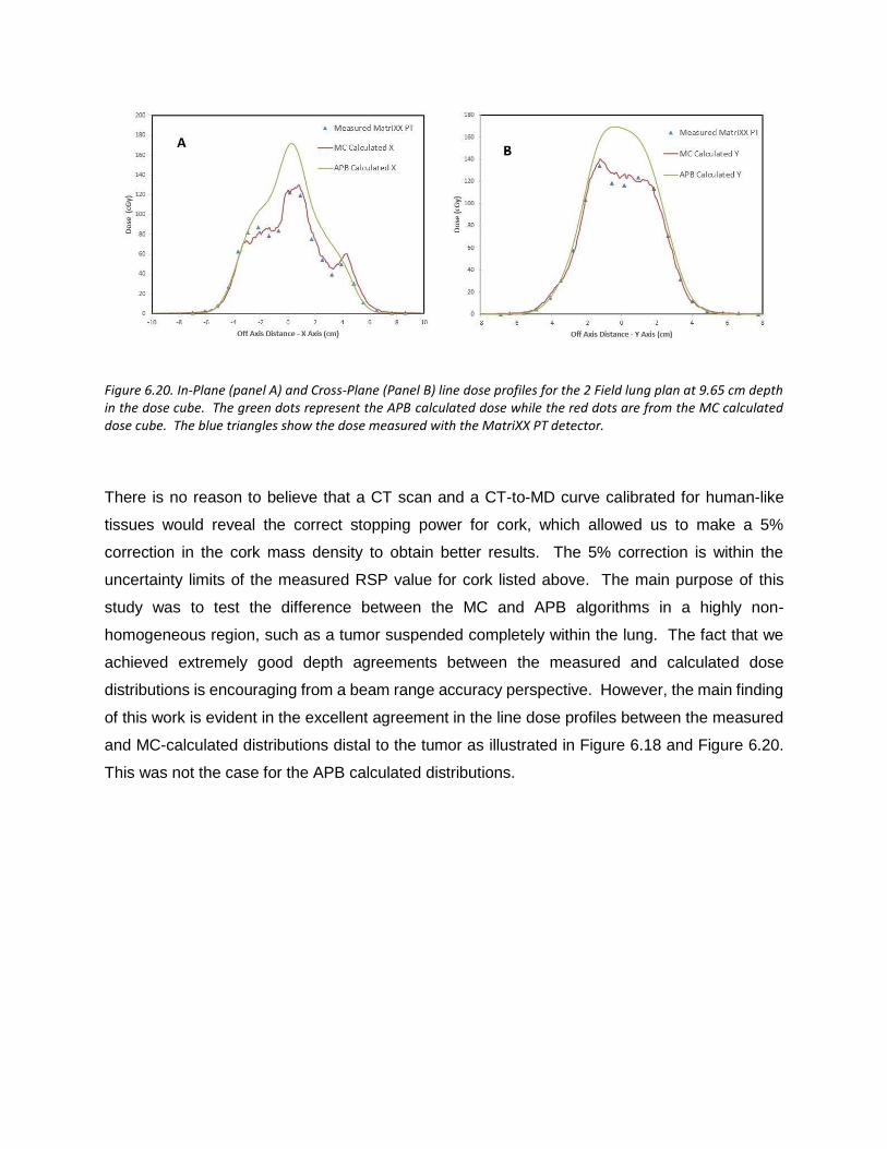
Figure 6.20. In-Plane (panel A) and Cross-Plane (Panel B) line dose profiles for the 2 Field lung plan at 9.65 cm depth in the dose cube. The green dots represent the APB calculated dose while the red dots are from the MC calculated dose cube. The blue triangles show the dose measured with the MatriXX PT detector.

There is no reason to believe that a CT scan and a CT-to-MD curve calibrated for human-like

tissues would reveal the correct stopping power for cork, which allowed us to make a 5%

correction in the cork mass density to obtain better results. The 5% correction is within the

uncertainty limits of the measured RSP value for cork listed above. The main purpose of this

study was to test the difference between the MC and APB algorithms in a highly non-

homogeneous region, such as a tumor suspended completely within the lung. The fact that we

achieved extremely good depth agreements between the measured and calculated dose

distributions is encouraging from a beam range accuracy perspective. However, the main finding

of this work is evident in the excellent agreement in the line dose profiles between the measured

and MC-calculated distributions distal to the tumor as illustrated in Figure 6.18 and Figure 6.20.

This was not the case for the APB calculated distributions.

Figure 6.21. Frequency distributions of the normalized number of voxels having a certain HU for two real lung tumors treated in our clinic and for the simulated lung tumor. The data is normalized to a maximum of 100 to accommodate the different volumes of the tumors evaluated.

6.3.7 Clinical Impact of Our Phantom

The ground meat simulating the tumor is a reasonable representation of a real solid tumor and is

readily separable to enable dose measurement inside the tumor. Lung tumors are mostly less

dense than soft tissue, which was achieved by using 70% lean ground meat as the tumor. We

reviewed the HUs of solid lung tumors of two patients we treated and found that the average HU

for the GTVs drawn for these patients was 35 + 26 which compared well with our simulated lung

tumor having a mean HU value of 46 + 21. The frequency distributions for two real lung tumors

and for the simulated lung tumor are shown in in Figure 6.21. The simplicity of this model may

be contrasted with an elaborate lung phantom involving a water-filled casing with porcine lung

[6.65], a commercial synthetic torso [6.66, 6.67], or a commercial pig organ phantom [6.68]. Users

of cork-based phantoms should be aware of potential discrepancies between their TPS and actual

stopping powers [6.69].

6.3.8. RaySearch Warnings

RaySearch informs the user that the pencil beam scanning dose engine uses the infinite slab

approximation thereby increasing error as a function of lateral inhomogeneity [6.70]. We

demonstrate this behavior, as shown in Figures 6.17 to 6.20. They strongly recommend using the

Monte Carlo dose engine for final dose computation. We concur based on the results shown in

this report.

6.3.9. Conclusions

We have created a novel phantom simulating a lung cancer tumor, representative of the typical

size and location of patient cases often treated in our clinic. This phantom enabled us to determine

the errors resulting from using an analytical pencil beam algorithm for lung targets. We were able

to demonstrate the superiority of the Monte Carlo dose calculation algorithm for lung targets. This

work also demonstrated how the infinite slab approximation used in the APB algorithm fails when

a distinct lateral inhomogeneity is encountered at the distal end of an otherwise fairly uniform

medium. The case represented in this phantom is, in our estimation, one of the worst cases that

one would encounter in the lung: namely, the tumor is not adjacent to the rib cage but rather

suspended in the lung. This represents many centrally located lung targets. In addition, the plans

created for this study were not created using robust optimization, something that would have

decreased the sensitivity to dose calculation error. Therefore, based on this work and supported

by many other authors referenced herein, we recommend that APB algorithms should not be used

for any lung targets, and that a Monte Carlo based algorithm should be used as the dose engine

for plan optimization and final dose calculation.

6.4. ACKNOWLEDGMENTS

We are grateful to RaySearch Americas Inc. and RaySearch Laboratories AB for their clinically

useful developments.

CHAPTER 7:

SUMMARY AND CONCLUDING REMARKS ON THE WORK

PRESENTED IN THIS THESIS.

7.1. EXECUTIVE SUMMARY

As stated in the BJR paper and the remainder of this chapter 5, I believe that many technologies

have come to fruition over the past years, but due to a lack of sales volume in the proton therapy

industry, vendors have not been able to implement the best technologies to benefit the total

treatment delivery process. Furthermore, due to the often very large debt burden on existing

facilities, there is often no money available to upgrade existing technologies or to implement

newer technologies at existing facilities. Providing that upright treatments get adopted into clinical

use, the costs of proton therapy facilities will be reduced dramatically with the subsequent benefit

of more facilities being built. This will provide the critical volume in the industry that will improve

the cost effectiveness of proton therapy in all aspects i.e. manufacturing, clinical use and

operations. As stated above the next generation systems must be designed such that all the

features listed in this chapter can be accommodated. This will allow for proton therapy systems

to function at a truly differentiating level and set proton therapy apart from the most advanced x-

ray therapy systems to the benefit of many cancer patients.

The next few years are crucial for the survival of proton therapy which I believe is essential and

must happen based on the excellent clinical results from the ever-increasing number of clinical

studies. The key issue is and will remain the cost of proton therapy systems. The proton therapy

industry ran into a brick wall from a cost perspective and even the most compact therapy systems

such as the half gantries offered by IBA, ProTom and Hitachi, the superconducting gantry offered

by ProNova and superconducting cyclotron mounted directly on a gantry offered by MeVion, still

require massive and expensive shielded bunkers that take a lot of time to construct. I believe this

brick wall situation is now forcing the industry to explore new cost saving avenues hence the

increased interest in upright treatments that LEO cancer care is experiencing. I have no doubt

that upright treatments are the future in radiation therapy and will allow for significant cost savings,

efficiency enhancements and for the implementation of the prerequisite technologies discussed

in this chapter.

Shifting the patient positioning and treatment paradigm away from the “modern” way of treating

patients in a lying down position back to the “traditional” way of treating in the upright position

might be counter intuitive and certainly not easy but is essential to reduce the cost of particle

therapy. The good news is that this paradigm shift is also supported by initial clinical evidence

that it will be advantageous to the patient from a patient comfort and anatomical perspective.

After all, the most important aspects to be considered in any form of medical treatment, are those

that have the most direct and immediate impact on the patient’s well-being e.g. patient comfort

and stress levels etc.

I would like to conclude this work with a story that has relevance to what we do in radiation therapy.

Somebody once asked Jack Nicklaus – how do you win in Augusta (the USA golf masters

tournament)? According to the story, he answered – “If you want to win in Augusta, you need to

start with the ball in the hole, then you figure out where to be on the green to get the ball in the

hole with one put, - then where do you need to be on the fairway to get to that spot on the green

and so you work you way back to the tee”. This is exactly what we should do in developing and

conducting radiation therapy. In the past, the emphasis was often on the beam and how to get

the beam to the patient rather than starting at the patient. I believe that upright treatments and

the focus on patient comfort and the improved patient positioning and beam delivery efficiencies

facilitated by this, are indeed following the “Augusta golf” principle.

REFERENCES

1.1. Wilson R. (1946) Radiological Use of Fast Protons. Radiology 47:487-491.

1.2. Das I, Harald P. (2015) Principles and Practice of Proton Beam Therapy. Medical Physics Publishing, Inc.

1.3. Koehler A, et al. (1972) Protons in Radiation Therapy. Radiology 104:191-195.

1.4. Kanai T, et al. (1980) Spot scanning system for proton radiotherapy. Medical Physics 7,365. Pedroni E, Bacher R, Blattmann H, et al. (1995) The 200-MeV Proton Therapy Project at the Paul Scherrer Institute: Conceptual Design and Practical Realization. Med Phys. 22(1):37-53.

1.5. Pedroni E, Bacher R, Blattmann H, et al. (1995) The 200-MeV Proton Therapy Project at the Paul Scherrer Institute: Conceptual Design and Practical Realization. Med Phys. 22(1):37-53.

1.6. Bortfeld TR, Loeffler JS. Three ways to make proton therapy affordable. Nature. 2017 Sep 25;549(7673):451453.

1.7. Baumann BC, Mitra N, Harton JG, et al. Comparative Effectiveness of Proton vs Photon Therapy as Part of Concurrent Chemoradiotherapy for Locally Advanced Cancer. JAMA Oncol. 2020;6(2):237–246. doi:10.1001/jamaoncol.2019.4889

1.8. MacDonald S, Jimenez R, Paetzold P, et al. (2013) Proton Radiotherapy for Chest Wall and Regional Lymphatic Radiation: Dose Comparisons and Treatment Delivery. Radiat Oncol. 8:71

1.9. D T L Jones, A N Schreuder, J E Symons and M Yudelev: The NAC Particle Therapy Facilities. Hadrontherapy in Oncology. (1994) 307.

1.10. Anferov, Vladimir, Ball, M, Berg, G.P, Broderick, B, Collins, J., East, G.,Friesel, D,Jenner, D,Jones, W.R, Katuin, J,Klein, Susan,Nelson, C, Schreuder, Niek, Self, J.. (2001). The Indiana University Midwest Proton Radiation Institute. 1. 645 - 647 vol.1. 10.1109/PAC.2001.98759.

2.1. Schreuder A N, Hedrick S G, Renegar J R, Netherton T J, Chen H, Blakey M D, Artz M E, Robison B H, Meek A G and Fagundes M, A Review of Proton Therapy and the Path to Widespread Clinical Adoption, Medical Physics international Journal. 2016; 4 (1): 35 – 46.

2.2. Beasley M, Driver D, Dobbs HJ. Complications of radiotherapy: improving the therapeutic index. Cancer Imaging. 2005;5(1):78–84. Published 2005 Jul 25. doi:10.1102/1470-7330.2005.0012

2.3. E. Rutherford, F.R.S.*The Scattering of α and β Particles by Matter and the Structure of the Atom. Philosophical Magazine, Series 6, vol. 21 May 1911, p. 669-688

2.4. W. H. Bragg M.A. & R. Kleeman B.Sc.; On the α particles of radium, and their loss of range in passing through various atoms and molecules The London, Edinburgh, and Dublin Philosophical Magazine and

Journal of Science, Pages 318-340 Published online: 16 Apr 2009. Download citation https://doi.org/ 10.1080/14786440509463378

2.5. E. O. Lawrence and M. S. Livingston, The Production of High Speed Light Ions Without the Use of High Voltages. Phys. Rev. 40, 19 – Published 1 April 1932

2.6. Wilson R. (1946) Radiological Use of Fast Protons. Radiology 47:487-491.

2.7. Tobias CA, Anger HO, Lawrence JH. Radiological use of high energy deuterons and alpha particles. Am J Roentgenol. 1952; 67:1–27.

2.8. Boone ML, Lawrence JH, Connor WG, et al. Introduction to the use of protons and heavy ions in radiation therapy: historical perspective. Int J Radiat Oncol Biol Phys. 1977; 3:65–9.

2.9. Tobias CA. Pretherapeutic investigations with accelerated heavy ions. Radiology. 1973; 108:145–58.

2.10. B Larsson, L Leksell, B Rexed, P Sourander, W Mair… The high-energy proton beam as a neurosurgical tool - Nature, 1958 – Springer

2.11. Larsson, B., Pretherapeutic physical experiments with high energy protons. British Journal of Radiology, 1961 - 34, 143- 51

2.12. Das I, Paganetti H. (2015) Principles and Practice of Proton Beam Therapy. Medical Physics Publishing, Inc.

2.13. Schreuder, A.N., Jones, D.T.L., Symons, J.E. et al. The NAC proton treatment planning system; Strahlenther Onkol (1999) 175(Suppl 2): 10. https://doi.org/10.1007/BF03038876

2.14. Schreuder AN, Jones DTL, Symons JE, et al. The NAC Proton Therapy Beam Delivery System. In: Cornell J Ed. Proc. 14th Conf on Cyclotrons and their Applications. Singapore: World Scientific Publishing, 1996:523–6.

2.15. Cormack AM “Representation of a function by its line integrals, with some radiological applications”, Journal of Applied Physics, 34(9): 2722-2727, 1963.

2.16. Hounsfield GN: Computerised transverse axial scanning (tomography) I. Description of system. Br J Radiol 46: 1016-1022, 1973.

2.17. Friedland GW, Thurber BD “The birth of CT”, American Journal of Roentgenology, 167:1365-1370, 1996.

2.18. Webb S “In the beginning”, The Physics of Medical Imaging, Institute of Physics Publishers, Bristol, UK, pp. 719, 1988.

2.19. GODFREY N. HOUNSFIELD, COMPUTED MEDICAL IMAGING; Nobel Lecture, 8 December 1979; The Medical Systems Department of Central Research Laboratories EMI, London, England

2.20. ALLAN M. CORMACK, EARLY TWO-DIMENSIONAL; RECONSTRUCTION AND RECENT TOPICS STEMMING FROM IT, Nobel Lecture, 8 December, 1979, Physics Department, Tufts University, Medford, Mass., U.S.A.

2.21. Goitein, M., Abrams, M. Multi-Dimensional Treatment Planning, I. Delineation of Anatomy. Int. J. Rad. Onc. Biol. Phys. Vol. 9, 777–787 (1983).

2.22. Goitein, M., Abrams, M., Rowell, D., Pollari, H., Wiles, J. Multi-Dimensional Treatment Planning, II. Beam's Eye View, Back Projection, and Projection Through CT Sections. Int. J. Rad. Onc. Biol. Phys. 9, 789–797, 1983.

2.23. Petti P. Differential-pencil-beam dose calculations for charged particles. Med Phys. 1992;19(1):137-49.

2.24. Hong L, Michael G, Bucciolini M, et al. A pencil beam algorithm for proton dose calculations. Phys Med Biol. 1996; 41:1305–1330.

2.25. Soukup M, Fippel M, Alber M. A pencil beam algorithm for intensity modulated proton therapy derived from Monte Carlo simulations. Phys Med Biol. 2005; 50:5089–5104.

2.26. Urie, M., Goitein, M., Holley, W. R., Chen, G. T. Y. Degradation of the Bragg Peak Due to Inhomogeneities. Phys. Med. Biol. 31, 1–15 (1986).

2.27. Urie, M. M., Sisterson, J. M., Koehler, A. M., Goitein, M., Zoesman, J. Proton Beam Penumbra, Effects of Separation Between Patient and Beam Modifying Devices. Med. Phys. 13, 734–41 (1986).

2.28. A N Schreuder, D T L Jones, J E Symons, T Fulcher and A Kiefer: The NAC Proton Therapy Beam Delivery System. Proc. 14th Int. Conf. on Cyclotrons and their Applications, Ed. J. Cornell, World Scientific, Singapore (1996) pp491-498.

2.29. V. Anferov, B. Broderick, J.C. Collins, D.L. Friesel, D. Jenner, W.P. Jones, J. Katuin, S.B. Klein, W. Starks, J. Self, N. Schreuder, The Midwest Proton Radiation Institute Project at the Indiana University Cyclotron Facility. Cyclotrons and their Applications, AIP 600 pp27-29 (2001).

2.30. Kanai T, et al. (1980) Spot scanning system for proton radiotherapy. Medical Physics 7,365.

2.31. Pedroni E, Bacher R, Blattmann H, Böhringer T, Coray A, Lomax A, Lin S, Munkel G, Scheib S, Schneider U, et al. The 200-MeV proton therapy project at the Paul Scherrer Institute: conceptual design and practical realization. Med Phys. 1995 Jan;22(1):37-53. PMID: 7715569

2.32. Pedroni E, Bearpark R, Böhringer T, Coray A, Duppich J, Forss S, George D, Grossmann M, Goitein G, Hilbes C, Jermann M, Lin S, Lomax A, Negrazus M, Schippers M, Kotle G.; The PSI Gantry 2: a second generation proton scanning gantry. Z Med Phys. 2004;14(1):25-34.

2.33. MacDonald S, Patel S, Hickey S, et al. (2013) Proton Therapy for Breast Cancer After Mastectomy: Early Outcomes of a Prospective Clinical Trial. Int J Radiat Oncol Biol Phys. 86(3):484-90.

2.34. MacDonald S, Jimenez R, Paetzold P, et al. (2013) Proton Radiotherapy for Chest Wall and Regional Lymphatic Radiation: Dose Comparisons and Treatment Delivery. Radiat Oncol. 8:71

2.35. Grassberger C, Dowdell S, Lomax A, et al., Motion Interplay as a Function of Patient Parameters and Spot Size in Spot Scanning Proton Therapy for Lung Cancer, Int J Radiat Oncol Biol Phys. 2013, 86(2): 380–386.

2.36. Frank S, Cox J, Gillin M, et al. (2014) Multi-field Optimization Intensity Modulated Proton Therapy for Head and Neck Tumors: A Translation to Practice. Int J Radiat Oncol Biol Phys. 89:846–53.

2.37. Liu W, Zhang X, Li Y, et al. (2012) Robust Optimization of Intensity Modulated Proton Therapy. Med Phys. 39(2):1079-91.

2.38. Paganetti, H. Monte Carlo Method to Study the Proton Fluence for Treatment Planning. Med. Phys. 25, 237– 5 (1998)

2.39. Paganetti, H. (2012) Range Uncertainties in Proton Therapy and the Role of Monte Carlo Simulations. Phys Med Biol. 57(11): R99-117.

2.40. Schreuder AN, Bridges DS, Rigsby L, Blakey M, Janson M, Hedrick SG, Wilkinson JB. Validation of the RayStation Monte Carlo dose calculation algorithm using realistic animal tissue phantoms. J Appl Clin Med Phys. 2019 Oct; 20(10):160-171. doi: 10.1002/acm2.12733. Epub 2019 Sep 21.

2.41. Schreuder AN, Bridges DS, Rigsby L, Blakey M, Janson M, Hedrick SG, Wilkinson JB. Validation of the RayStation Monte Carlo dose calculation algorithm using a realistic lung phantom. J Appl Clin Med Phys. 2019 Dec; 20(12):127-137. doi: 10.1002/acm2.12777. Epub 2019 Nov 25.

2.42. Schreuder AN, Shamblin J. Proton therapy delivery: what is needed in the next ten years? Br J Radiol. 2019 Nov 14:20190359. doi: 10.1259/bjr.20190359. [2. Epub ahead of print] PMID: 31692372

2.43. Yan S, Lu H, Flanz J, Adams J, Trofimov A, Bortfeld T. Reassessment of the Necessity of the Proton Gantry: Analysis of Beam Orientations From 4332 Treatments at the Massachusetts General Hospital Proton Center Over the Past 10 Years. Int J Radiat Oncol Biol Phys, 2016 May 1;95(1):224-233. doi: 10.1016/j.ijrobp.2015.09.033. Epub 2015 Sep 30. PMID: 26611874.

3.1. C Stannard, F Vernimmen, D Jones, J Wilson, L van Wijk, S Brennan, A N Schreuder, J Symons, V Levin, E Mills, A Alberts, D Werner, B Smit and G Schmitt: The Neutron and Proton Therapy Programmes at the National Accelerator Centre: Preliminary Results. Radiother. Oncol. Invest. 2 (1995) 245-255

3.2. Maor M.H. (1988) Fast Neutron Therapy: Problems and Promise. In: Withers H.R., Peters L.J. (eds) Innovations in Radiation Oncology. Medical Radiology (Diagnostic Imaging and Radiation Oncology). Springer, Berlin, Heidelberg; DOI https://doi.org/10.1007/978-3-642-83101-0-25

3.3. M. J. Berger, "ESTAR, PSTAR, and ASTAR: Computer Codes for Calculating Stopping Power and Range Tables for Electrons, Protons, and Helium Ions," National Institute of Standards and Technology Report, NISTIR 4999, (1992) (RSIC PSR-330).

3.4. A.M. Koehler, R.J. Schneider and J.M. Sisterson, ‘Flattening of proton dose distributions for large-field radiotherapy,’ Med. Phys. 4(4) (1977) 297-301.

3.5. P.J. Binns and J.H. Hough, ‘Secondary dose exposures during 200 MeV proton therapy,’ Rad. Prot. Dosim. 70 (1997) 441 – 444

3.6. B. Gottschalk, “BGtalks: Multi-Layer Faraday Cup” (2007), available at “https://github.com/ BernardGottschalk/BG-distribution”

3.7. Hansen P, Hu D. An isocenter estimation tool for proton gantry alignment. Rev Sci Instrum 2017; 88(12):125102.

3.8. W. T. Chu, B. A. Ludewigt and T. R. Renner. Instrumentation for treatment of cancer using proton and light ion beams, Review of Scientific Instruments 64, 2055 (1993); https://doi.org/10.1063/1.1143946

3.9. A N Schreuder, et al. Three years' experience with the NAC proton therapy patient positioning system. Advances in Hadrontherapy, Eds. U Amaldi, B Larsson and Y Lemoigne, Elsevier BV, Amsterdam (1997) pp 251-258.

3.10. Van der Vlugt G and Rüther H. A real-time photogrammetric system for patient positioning in proton therapy. Int. Arch. Photogramm. and Rem. Sens. 1992; 28: 880-885.11

3.11. A N Schreuder, D T L Jones and A Kiefer. A small ionization chamber for dose distribution measurements in a clinical proton beam. Advances in Hadrontherapy, Eds. U Amaldi, B Larsson and Y Lemoigne, Elsevier BV, Amsterdam (1997) pp 284-289.

3.12. R. E. Pollock, "The Indiana University Cyclotron Facility (IUCF) 1980," in IEEE Transactions on Nuclear Science, vol. 28, no. 2, pp. 1433-1436, April 1981.doi: 10.1109/TNS.1981.4331435

3.13. Anferov, Vladimir, Ball, M, Berg, G.P, Broderick, B, Collins, J., East, G.,Friesel, D,Jenner, D,Jones, W.R, Katuin, J,Klein, Susan,Nelson, C, Schreuder, Niek, Self, J.. (2001). The Indiana University Midwest Proton Radiation Institute. 1. 645 - 647 vol.1. 10.1109/PAC.2001.987593.

3.14. Klein, Susan B, Status of the Proton Therapy Project at IUCF and the Midwest Proton Radiotherapy Institute. AIP Conference Proceedings. 680, 1081 (2003); https://doi.org/10.1063/1.1619895.

3.15. D.L. Friesel, T.J.P. Ellison, T. Sloan, and M. Ball; MULTIPLE BEAM OPERATIONS AT IUCF', Twelfth International Conference on Cyclotrons and their Applications, Berlin, Germany, 8 – 12 May 1989, , P380- 383, https://doi.org/10.1142/0990

3.16. Grusell, Erik & Montelius, Anders & Brahme, Anders & Rikner, G & Russell, K. (1995). A general solution to charged particle beam flattening using an optimized dual-scattering-foil technique, with application to proton therapy beams. Physics in medicine and biology. 39. 2201-16. 10.1088/0031-9155/39/12/005.

3.17. B. Gottschalk, “BGtalks: Double scattering” (2007); available at “https://github.com/ BernardGottschalk/ BG-distribution”.

3.18. Anferov V. Combined X-Y scanning magnet for conformal proton radiation therapy. Med Phys. 2005 Mar; 1932(3):815-8.

3.19. Verhey L, (Chairman), Blattman H, DeLuca, P.M., Miller, D., clinical proton dosimetry Part I: Beam production, beam delivery and measurement of absorbed dose. Report 59 of the international cominission on radiation units and measurements, (ICRU), Bethesda, MD, 53 pp. 1998.

3.20. Vynckier, S., Bonnett, D.E., Jones, D.T.L. Code of practice for clinical proton dosimetry. Radiother. Oncol. 1991; 20:53–63.

3.21. J. Katuin, N. Schreuder, The Use of Industrial Robot Arms for High Precision patient Positioning. Proc. CAARI 2002, Denton TX, Nov. (2002)

3.22. Mazal A, Rosenwald J.C., Ferrand R., Delacroix S., Nauraye C., Aligne C., Schlienger P., Habrand J.L. “Robots In High Precision Patient Positioning For Conformal Radiotherapy” Proceedings of World Congress on Medical Physics and Biomedical Engineering, Medical & Biological Engineering & Computing, Nice, September 1997, 35, pp. 824

3.23. Ferrand, R., Mazal, A., Aligne, S., Delacroix, S., Nauraye, C., Rosenwald, J.C., Hierso, E., Habrand, J.L. “Patient Positioning system at CPO: test and commissioning”, Abstracts of the XXVI PTCOG Meeting, edited by Sisterson, Boston MA.

3.24. Allgower CE, Schreuder A N, Farr JB, Mascia AE., Experiences with an application of industrial robotics for accurate patient positioning in proton radiotherapy. Int J Med Robot. 2007 Mar; 3:72-81. Review.

3.25. A N Schreuder, et al. The Non-orthogonal Fixed Beam Arrangement for the Second Proton Therapy Facility at the National Accelerator Centre. CP475, Applications of Accelerators in Research and Industry, Eds J L Duggan and I L Morgan, The American Institute of Physics, (1999) pp 963-966.

3.26. Sommer A: Industrial Robots for Patient Support. In Ion Beam Therapy, Biological and Medical Physics, Biomedical Engineering. Edited by: Linz U. Berlin Heidelberg: Springer-Verlag; 2012:559-577.

4.1. Pflugfelder D., Wilkens J. J., and Oelfke U., “Worst case optimization: a method to account for uncertainties in the optimization of intensity modulated proton therapy,” Phys. Med. Biol. 53, 1689–1700 (2008).10.1088/0031-9155/53/6/013

4.2. Unkelbach J., Bortfeld T., Martin B. C., and Soukup M., “Reducing the sensitivity of IMPT treatment plans to setup errors and range uncertainties via probabilistic treatment planning,” Med. Phys. 36, 149–163 (2009).10.1118/1.3021139

4.3. Coutrakon G, Cortese J, Ghebremedhin A, et al. (1997) Microdosimetry spectra of the Loma Linda proton beam and relative biological effectiveness comparisons. Medical Physics 24:1499 DOI 10.1118/1.598038.

4.4. Moyers M, Miller D, Bush D. (2001) Methodologies and Tools for Proton Beam Design for Lung Tumors. Int J Radiat Oncol Biol Phys. 49 (5):1429-1438.

4.5. T. Landberg, J. Chavaudra, J. Dobbs, J. -P. Gerard, G. Hanks, J. -C. Horiot, K. -A. Johansson, T. Möller, J. Purdy, N. Suntharalingam, H. Svensson, Report 62, Journal of the International Commission on Radiation Units and Measurements, Volume os32, Issue 1, November 1999, Page NP, https://doi.org/ 10.1093/jicru/os32.1.Report62

4.6. Yuh, G, Loredo L, et al. (2004) Reducing Toxicity from Craniospinal Irradiation: Using Proton Beams to Treat Medulloblastoma in Young Children. Cancer J. 10(6):386-90.

4.7. St. Clair, W H, Adams, J A, Bues, M, et al. (2004) Advantage Of Protons Compared To Conventional X-Ray Or IMRT In The Treatment Of A Pediatric Patient With Medulloblastoma. Int J Radiat Oncol Biol Phys. 58(3):72734.

4.8. Lin H, Ding X, Kirk M, et al. (2014) Supine Craniospinal Irradiation Using a Proton Pencil Beam Scanning Technique Without Match Line Changes for Field Junctions. Int J Radiat Oncol Biol Phys. 90(1):71-8.

4.9. De Laney T, Kooy H, (2008) Proton and Charged Particle Radiotherapy. Lippincott, Williams, & Wilkins, Philadelphia.

4.10. Ahn P, Sharma S, Zhou O. (2015) A Comparative Quality of Life Cohort of Oropharyngeal Squamous Cell (OPSCC) Patients Treated With Volumetric Modulated Radiation Therapy (VMAT) Versus Proton Pencil Beam Scanning (PBS). Int J Radiat Oncol Biol Phys. (93): S71.

4.11. Whelan T, Pignol J, Levine M, et al. (2010) Long-Term Results of Hypofractionated Radiation Therapy for Breast Cancer. N Engl J Med 362(6):513-20.

4.12. Xu N, Ho M, Li Z, et al. (2013) Can Proton Therapy Improve the Therapeutic Ratio in Breast Cancer Patients at Risk for Nodal Disease? Am J Clin Oncol. 37(6):568-74.

4.13. Chang J, Komaki R, Lu C, et al. (2011) Phase 2 Study of High-Dose Proton Therapy with Concurrent Chemotherapy for Unresectable Stage III Nonsmall Cell Lung Cancer. Cancer. 117:4707-4713.

4.14. Chang J, Li H, Zhu X, et al. (2014) Clinical Implementation of Intensity Modulated Proton Therapy for Thoracic Malignancies. Int J Radiat Oncol Biol Phys. 90(4): 809–818.

4.15. Darby S, Ewertz M, McGale P, et al. (2013) Risk of Ischemic Heart Disease in Women after Radiotherapy for Breast Cancer. N Engl J Med. 368(11):987-98.

4.16. Fagundes M, Robison B, et al. (2015) Intensity Modulated Proton Therapy in the Treatment of High-Risk Prostate Cancer: How Do Robustly Optimized Proton Plans Compare With Volumetric Modulated Arc Therapy? ASTRO.

4.17. Fagundes M, Robison B, et al. (2015) High-Dose Rectal Sparing With Trans Perineal Injection of Hydrogel Spacer in Intensity Modulated Proton Therapy for Localized Prostate Cancer. Int J Radiat Oncol Biol Phys. 93(3): E230.

4.18. Bryant C, Smith T, Henderson R, et al. (2016) Five-Year Biochemical Results, Toxicity, and Patient-Reported Quality of Life After Delivery of Dose-Escalated Image Guided Proton Therapy for Prostate Cancer. Int J Radiation Oncol Biol Phys. 95(1):422-434.

4.19. Quan E, Liu W, Wu R, et al. (2013) Preliminary Evaluation of Multifield and Single-Field Optimization for the Treatment Planning of Spot-Scanning Proton Therapy of Head and Neck Cancer. Med Phys. 40: 081709.

4.20. Little M, Schipper M, Feng F, et al. (2012) Reducing Xerostomia after Chemo-IMRT for Head-and-Neck Cancer: Beyond Sparing the Parotid Glands. Int J Radiat Oncol Biol Phys. 83:1007.

4.21. Langendijk J, Doornaert P, Verdonck-de Leeuw I, et al. (2008) Impact of late treatment- related toxicity on quality of life among patients with head and neck cancer treated with radiotherapy. J Clin Oncol. 26: 3770–6.

5.1. Takahashi S, Conformation radiotherapy. Rotation techniques as applied to radiography and radiotherapy of cancer. Acta Radiol Diagn (Stockh). 1965;S242.

5.2. Brahme A, Roos JE, Lax I. Solution of an integral equation encountered in radiation therapy. Phys Med Biol 1982;27:1221–9.

5.3. Yu CX, Symons MJ, Du MN, Martinez AA, Wong JW. A method for implementing dynamic photon beam intensity modulation using independent jaws and multileaf collimator. Phys Med Biol 1995;40:769-787.

5.4. Yu CX, Li XA, Ma L, Chen D, Naqvi S, Shepard D, et al. Clinical implementation of intensity-modulated arc therapy. Int J Radiat Oncol Biol Phys 2002;53:453–63.

5.5. Deasy JO, Shepard D, Mackie TR. Distal edge tracking: A proposed delivery method for conformal proton therapy using intensity modulation. In: Leavitt DD, Starkschall G. (eds.) ICCR 1997: Proceedings of the XIIth International Conference on the use of Computers in Radiation Therapy at Salt Lake City. Madison, WI: Medical Physics Publishing; 1997.

5.6. Sandison GA, Papiez E, Bloch C, Morphis J. Phantom assessment of lung dose from proton arc therapy. Int J Radiat Oncol Biol Phys 1997;38(4):891-897.

5.7. Mackie TR, Holmes T, Swerdloff S, Reckwerdt P, Deasy JO, Yang J, et al. Tomotherapy: a new concept for the delivery of dynamic conformal radiotherapy. Med Phys 1993;20:1709–19.

5.8. Welsh JS, Patel RR, Ritter MA, Harari PM, Mackie TR, Mehta MP. Helical tomotherapy: an innovative technology and approach to radiation therapy. Technol Cancer Res Treat. 2002;1(4):311–5.

5.9. Mackie TR. History of tomotherapy. Phys Med Biol 2006;51:R427–53.

5.10. Teoh M, Clark CH, Wood K, Whitaker S, Nisbet A. Volumetric modulated arc therapy: a review of current literature and clinical use in practice. Br J Radiol 2011;84(1007):967-95.

5.11. Carabe-Fernandez A, Kirk M, Sanchez-Parcerisa D, Fager M, Burgdorf B, Stowe M, et al. Proton Modulated Arc Therapy Using Scanned Pencil Beams. Med Phys 2015;42(6):3483-3483.

5.12. Han W, Cao F, Chen MB, Lu RZ, Wang HB, Yu M, et al. Prognostic Value of SPARC in Patients with Pancreatic Cancer: A Systematic Review and Meta-Analysis. PLoS One 2016;11(1):e0145803.

5.13. Seco J, Gu G, Marcelos T, Kooy H, Willers H. Proton arc reduces range uncertainty effects and improves conformality compared with photon volumetric modulated arc therapy in stereotactic body radiation therapy for non-small cell lung cancer. Int J Radiat Oncol Biol Phys 2013;87(1):188-194.

5.14. Langner UW, Eley JG, Guerrero M, Langen K, Mossahebi S, Zhu M, D'Souza W, Yi B. A method to deliver energy modulated planar proton arc therapy (EMPPAT). Jour Proton Ther. 2017; 3:312. DOI: 10.14319/jpt.31.2

5.15. Ding X, Li X, Qin A, Zhou J, Yan D, Stevens C, et al. Have we reached proton beam therapy dosimetric limitations? – A novel robust, delivery-efficient and continuous spot-scanning proton arc (SPArc) therapy is to improve the dosimetric outcome in treating prostate cancer. Acta Oncol 2018;57(3):435-437.

5.16. Ding X, Li X, Zhang JM, Kabolizadeh P, Stevens C, Yan D. Spot-Scanning Proton Arc (SPArc) Therapy: The First Robust and Delivery-Efficient Spot-Scanning Proton Arc Therapy. Int J Radiat Oncol Biol Phys 2016;96(5):11071115.

5.17. Poludniowski G, Allinson NM, Evans PM. Proton radiography and tomography with application to proton therapy. Br J Radiol 2015;88(1053):20150134.

5.18. Giantsoudi D, Grassberger C, Craft D, Niemierko A, Trofimov A, Paganetti H. Linear energy transfer-guided optimization in intensity modulated proton therapy: feasibility study and clinical potential. Int J Radiat Oncol Biol Phys 2013;87(1):216-22.

5.19. Grassberger C, Trofimov A, Lomax A, Paganetti H. Variations in linear energy transfer within clinical proton therapy fields and the potential for biological treatment planning. Int J Radiat Oncol Biol Phys. 2011;80(5):1559-1566. doi:10.1016/j.ijrobp.2010.10.027

5.20. Favaudon V, Fouillade C, Vozenin MC. Ultrahigh dose-rate, "flash" irradiation minimizes the side-effects of radiotherapy. Cancer Radiother 2015;19(6-7):526-31.

5.21. Patriarca A, Fouillade C, Auger M, Martin F, Pouzoulet F, Nauraye C, et al. Experimental Set-up for FLASH Proton Irradiation of Small Animals Using a Clinical System. Int J Radiat Oncol Biol Phys 2018;102(3):619-626

5.22. Girdhani S, Abel E, Katsis A, Rodriquez A, Senapati S, KuVillanueva A, et al. LB-280 / 26 - FLASH: A novel paradigm changing tumor irradiation platform that enhances therapeutic ratio by reducing normal tissue toxicity and activating immune pathways. In: Dang VC, Quong JN. (eds.) Proceedings of the 110th Annual Meeting of the American Association for Cancer Research; 2019 March 29 - April 3; Atlanta, GA. Philadelphia (PA): AACR; 2019. Abstract nr. LB-280

5.23. Buonanno M, Grilj V, Brenner DJ. Biological effects in normal cells exposed to FLASH dose rate protons.

Radiother Oncol . 2019;139:51-55. doi:10.1016/j.radonc.2019.02.009.

5.24. Zenklusen SM1, Pedroni E, Meer D, Bula C, Safai S. Preliminary investigations for the option to use fast uniform scanning with compensators on a gantry designed for IMPT. Med Phys. 2011 Sep;38(9):5208-16. doi: 10.1118/1.3626483.

5.25. Courneyea L, Beltran C, Tseung HS, Yu J, Herman, MG. Optimizing mini-ridge filter thickness to reduce proton treatment times in a spot-scanning synchrotron system. Med Phys 2014;41:061713.

5.26. Knopf AC, Lomax A. In vivo proton range verification: a review. Phys Med Biol 2013;58:R131–R160.

5.27. Parodi K, Polf JC. In vivo range verification in particle therapy. Med Phys 2018;45:e1036-e1050. Available from: https://aapm.onlinelibrary.wiley.com/doi/full/10.1002/mp.12960 doi: 10.1002/mp.12960

5.28. Hueso-González F, Rabe M, Ruggieri TA, Bortfeld T, Verburg JM. A full-scale clinical prototype for proton range verification using prompt gamma-ray spectroscopy. Phys Med Biol 2018;63(18):185019.

5.29. Koehler AM. Proton radiography. Science. 1968;160:303–4. Available from: http://science.sciencemag. org/ content/160/3825/303 doi: 10.1126/science.160.3825.303

5.30. Cormack AM, Koehler AM. Quantitative proton tomography: preliminary experiments. Phys Med Biol 1976;21:560–9. Available from: https://iopscience.iop.org/article/10.1088/0031-9155/21/4/007/meta doi: 10.1088/0031-9155/21/4/007

5.31. Schneider U, Pedroni E. Proton radiography as a tool for quality-control in proton therapy. Med Phys 1995;22:353–63. Available from: https://aapm.onlinelibrary. wiley.com/ doi/abs/10.1118/1.597470 doi: 10.1118/ 1.597470

5.32. Pankuch M, Dejongh E, Dejongh F, Rykalin V, Karonis N, Ordonez C, et al. O115: A method to evaluate the clinical utility of proton radiography for geometric patient alignment. Proceedings of the 57 Annual Meeting of the Particle Therapy Cooperative Group (PTCOG). International Journal of Particle Therapy: Fall 2018, Vol. 5, No. 2, pp. 58-229. https://doi.org/10.14338/2331-5180-5-2-000

5.33. Plautz TE, Bashkirov V, Giacometti V, Hurley RF, Johnson RP, Piersimoni P, et al. An evaluation of spatial resolution of a prototype proton CT scanner. Med Phys 2016;43(12):6291-6300. Available from: https://aapm.onlinelibrary.wiley.com/ doi/abs/10.1118/1.4966028 doi: 10.1118/ 1.4966028

5.34. Dejongh E, Dejongh F, Rykalin V, Welsh J. Proton Residual Range Reconstruction and Impact on Dose to the Target Object in a Proton Imaging System. Available from:

http://www.protonvda.com/wpcontent/ uploads/2016/06/protonvda-ptcog-2016-2.pdf

5.35. Yan D, Vicini F, Wong J, Martinez A. Adaptive radiation therapy. Phys Med Biol 1997;42: 123–132.

5.36. Palacios MA, Bohoudi O, Bruynzeel AME, Koste JRVS , Cobussen P, Slotman BJ, et al. Role of Daily Plan Adaptation in MR-Guided Stereotactic Ablative Radiation Therapy for Adrenal Metastases. Int J Radiat Oncol Biol Phys 2018;102(2):426-433.

5.37. Bray F, Ferlay J, Soerjomataram I, Siegel RL, Torre LA, Jemal A. Global cancer statistics 2018: GLOBOCAN estimates of incidence and mortality worldwide for 36 cancers in 185 countries. CA Cancer J Clin 2018;68(6):394–424.

5.38. Ferlay J, Colombet M, Soerjomataram I, Mathers C, Parkin DM, Piñeros M, et al. Estimating the global cancer incidence and mortality in 2018: GLOBOCAN sources and methods. Int J Cancer 2019;144(8):1941–1953.

5.39. Keall PJ, Mageras GS, Balter JM, Emery RS, Forster KM, Jiang SB, et al. The management of respiratory motion in radiation oncology report of the AAPM Task Group 76. Med Phys 2006;33(10):3874–3900. Available from: https://aapm.onlinelibrary.wiley.com/ doi/full/10.1118/ 1.2349696 doi: 10.1118/1.2349696

5.40. Pollock S, Keall R, Keall P. Breathing guidance in radiation oncology and radiology: A systematic review of patient and healthy volunteer studies. Med Phys 2015;5490–5509. Available from: https://aapm.onlinelibrary.wiley.com/doi/full/10.1118/1.4928488 doi: 10.1118/1.4928488

5.41. Lewis GF, Gatto RG, Porges SW. A novel method for extracting respiration rate and relative tidal volume from infrared thermography. Psychophysiology 2011;48:877–887.

5.42. Pereira CB, Czaplik M, Blazek V, Leonhardt S, Teichmann D. Monitoring of Cardiorespiratory Signals Using Thermal Imaging: A Pilot Study on Healthy Human Subjects. Sensors (Basel) 2018;18(5): 1541. doi: 10.3390/s18051541

5.43. Laaksomaa M, Sarudis S, Rossi M, Lehtonen T, Pehkonen J, Remes J, et al. AlignRT® and Catalyst™ in wholebreast radiotherapy with DIBH: Is IGRT still needed? J Appl Clin Med Phys 2019;20(3):97-104. doi: 10.1002/acm2.12553.

5.44. Safai S, Bortfeld T, Engelsman M. Comparison between the lateral penumbra of a collimated double-scattered beam and uncollimated scanning beam in proton radiotherapy. Phys Med Biol 2008;53(6):1729-50. doi: 10.1088/0031-9155/53/6/016

5.45. Hyer DE, Hill PM, Wang D, Smith BR, Flynn RT. A dynamic collimation system for penumbra reduction in spotscanning proton therapy: proof of concept. Med Phys 2014;41(9):091701. doi: 10.1118/1.4837155

5.46. Hyer DE, Hill PM, Wang D, Smith BR, Flynn RT. Effects of spot size and spot spacing on lateral penumbra reduction when using a dynamic collimation system for spot scanning proton therapy. Phys Med Biol 2014;59(22):n187-96. doi: 10.1088/0031-9155/59/22/n187

5.47. Kang M, Chen H, Cessac R, Pang D. O 044: Commissioning of a Unique Penumbra Sharpening Adaptive Aperture of HYPERSCAN. Proceedings of the 57 Annual Meeting of the Particle Therapy Cooperative Group (PTCOG). International Journal of Particle Therapy: Fall 2018, Vol. 5, No. 2, pp. 58-229. https://doi.org/10.14338/2331-5180-5-2-000

5.48. Bues M, Newhauser WD, Titt U, Smith AR, Therapeutic step and shoot proton beam spot-scanning with a multi-leaf collimator: a Monte Carlo study, Radiation Protection Dosimetry, Volume 115, Issue 1-4, 20 December 2005, Pages 164–169, https://doi.org/10.1093/rpd/nci259

5.49. Winterhalter C, Lomax A, Oxley D, Weber DC, Safai S. A study of lateral fall-off (penumbra) optimisation for pencil beam scanning (PBS) proton therapy. Phys Med Biol 2018;63(2):1361-6560.

5.50. Meier G, Leiser D, Besson R, Mayor A, Safai S, Weber DC, et al. Contour scanning for penumbra improvement in pencil beam scanned proton therapy. Phys Med Biol 2017;62(6):2398-2416.

5.51. Tang X, Wang B, Rong Y. Artificial intelligence will reduce the need for clinical medical physicists. J Appl Clin Med Phys 2018;19(1):6-9.

5.52. Cardan RA, Popple RA, Fiveash J. A priori patient-specific collision avoidance in radiotherapy using consumer grade depth cameras. Med Phys 2017;44(7):3430-3436.

5.53. Farr JB, Flanz JB, Gerbershagen A, Moyers MF. New horizons in particle therapy systems. Med Phys 2018;45(11):e953-e983.

5.54. Cameron J, Schreuder N. Smaller – lighter – cheaper: new technological concepts in proton therapy. In: Linz U, editor. Ion Beam Therapy: Fundamentals, Technology, Clinical Applications. Berlin, Germany: SpringerVerlag, 2012: 673–85.

5.55. Pedroni E, Bearpark R, Böhringer T, Coray A, Duppich J, Forss S, et al. The PSI Gantry 2: a second generation proton scanning gantry. Zeitschrift für Medizinische Physik 2004; 14: 25–34. doi: https:// doi. org/ 10. 1078/ 0939-3889- 00194

5.56. Zhao T1, Sun B, Grantham K, Rankine L, Cai B, Goddu SM, Santanam L, Knutson N, Zhang T, Reilly M, Bottani B, Bradley J, Mutic S, Klein EE.; Commissioning and initial experience with the first clinical gantry-mounted proton therapy system. J Appl Clin Med Phys. 2016 Mar 8;17(2):24-40. doi: 10.1120/jacmp.v17i2.5868.

5.57. Pidikiti R, Patel BC, Maynard MR, Dugas JP, Syh J, Sahoo N, et al. Commissioning of the world's first compact pencil-beam scanning proton therapy system. J Appl Clin Med Phys 2018; 19: 94–105. doi: https:// doi. org/ 10. 1002/ acm2. 12225

5.58. Corke P I. VISUAL CONTROL OF ROBOT MANIPULATORS – A REVIEW; World Scientific Series in Robotics and Intelligent Systems, Visual Servoing, pp. 1-31 (1993) https://doi.org/ 10.1142/ 9789814503709_0001.

5.59. Frazzoli E, Dahleh M A, and Feron E, Real-Time Motion Planning for Agile Autonomous Vehicles; Journal of Guidance, Control, and Dynamics, 2002 25:1, 116-129.

5.60. Sueyoshi M., Olch A. J., Liu K. X., Chlebik A., Clark D., Wong K. W., Eliminating Daily Shifts, Tattoos, and Skin Marks: Streamlining Isocenter Localization With Treatment Plan Embedded Couch Values for External Beam Radiation Therapy, Practical Radiation Oncology, Volume 9, Issue 1, 2019, Pages e110-e117, ISSN 1879-8500, https://doi.org/10.1016/j.prro.2018.08.011.

5.61. Kügele, M., Mannerberg, A., Nørring Bekke, S., Alkner, S., Berg, L., Mahmood, F., Thornberg, C., Edvardsson, A., Bäck, S.Å.J., Behrens, C.F. and Ceberg, S. (2019), Surface guided radiotherapy (SGRT) improves breast cancer patient setup accuracy. J Appl Clin Med Phys, 20: 61-68. doi:10.1002/acm2.12700.

5.62. Stanton, D. Neutron Therapy Facility resumes treating patients. FermilabToday, January 20, 2006. Fermilab National Accelerator Laboratory,Office of Science/U.S. Department of Energy.

5.63. Shah, Anand P. et al. Upright 3D Treatment Planning Using a Vertical CT, Medical Dosimetry, Volume 34, Issue 1, 82 - 86

5.64. J.M. Denis, J.P. Meulders, E. Lannoye, Y. Longrée, G. Ryckewaert, F. Richard, S. Vynckier, A. Wambersie, The multileaf collimator for fast neutron therapy at Louvain-la-Neuve, Bulletin du Cancer/Radiothérapie, Volume 83, Supplement 1,1996,Pages 160s-169s,ISSN 0924 4212, https://doi.org/10.1016/0924-4212(96)84904-8.

5.65. Austin-Seymour M1, Caplan R, Russell K, Laramore G, Jacky J, Wootton P, Hummel S, Lindsley K, Griffin T. Impact of a multileaf collimator on treatment morbidity in localized carcinoma of the prostate. Int J Radiat Oncol Biol Phys. 1994 Dec 1;30(5):1065-71.

5.66. Farr J B, Maughan R L, Yudelev M, Blosser E, Brandon J, Horste T, Forman JD., Radiologic validation of a fast neutron multileaf collimator. Med Phys. 2007 Sep;34(9):3475-84.

5.67. Verhey LJ, Goitein M, McNulty P, Munzenrider JE, Suit HD. Precise positioning of patients for radiation therapy. Int J Radiat Oncol Biol Phys. 1982 Feb;8(2):289-94.

5.68. McCarroll, R.E., Beadle, B.M., Fullen, D., Balter, P.A., Followill, D.S., Stingo, F.C., Yang, J. and Court, L.E. (2017), Reproducibility of patient setup in the seated treatment position: A novel treatment chair design. J Appl Clin Med Phys, 18: 223-229. doi:10.1002/acm2.12024

5.69. Yang J, Chu D, Dong L, Court LE. Advantages of simulating thoracic cancer patients in an upright position. Pract Radiat Oncol. 2014;4:e53–e58.2.

5.70. Stanton, D. Neutron Therapy Facility resumes treating patients. FermilabToday, January 20, 2006. Fermilab National Accelerator Laboratory,Office of Science/U.S. Department of Energy.

5.71. Shah, Anand P. et al. Upright 3D Treatment Planning Using a Vertical CT, Medical Dosimetry, Volume 34, Issue 1, 82 - 86

5.72. Castro, Joseph R.Quivey, Jeanne M. et al. Clinical experience and expectations with helium and heavy ion irradiation, Int. J. Radiat. Oncol. Biol. Phys., 1977;3: 127 – 131.

5.73. Chen GT, Singh RP, Castro JR, Lyman JT, Quivey JM. Treatment planning for heavy ion radiotherapy. Int J Radiat Oncol Biol Phys. 1979 Oct;5(10):1809-19.

5.74. Tadashi Kamada, Hirohiko Tsujiia, Jun-Etsu Mizoe et. al. A horizontal CT system dedicated to heavy-ion beam treatment. Radiotherapy and Oncology 50 (1999) 235-237

5.75. Hayes, Ashley R.; Gayzik, F. Scott; Moreno, Daniel P.; Martin, R. Shayn; Stitzel, Joel D., Comparison of Organ Location, Morphology, and Rib Coverage of a Midsized Male in the Supine and Seated Positions; Computat Math Methods Med. 2013;2013:419821

5.76. Reiff, J.E.; Warner-Wasik, M.; Valicenti, R.K.; et al. Changes in the size and location of kidneys from the supine to standing positions and the implications for block placement during total body irradiation. Int. J. Radiat. Oncol. Biol. Phys. 45:447–9; 1999.

5.77. Abdulaziz M, Kavanagh A, Stothers L, Macnab AJ. Relevance of open magnetic resonance imaging position (sitting and standing) to quantify pelvic organ prolapse in women. Can Urol Assoc J. 2018;12(11):E453–E460. doi:10.5489/cuaj.5186

6.1. Durante M, Orecchia R, Loeffler JS. Charged-particle therapy in cancer: clinical uses and future perspectives. Nat Rev Clin Oncol. 2017 Aug;14(8):483-496. doi: 10.1038/nrclinonc.2017.30. Epub 2017 Mar 14. PMID: 28290489.

6.2. Particle Therapy Co-Operative Group. Particle therapy facilities in operation. Particle Therapy Co-Operative Group. 2018. Available at: https://ptcog.ch/index.php/facilities-in-operation. Accessed November 29, 2018.

6.3. Bortfeld TR, Loeffler JS. Three ways to make proton therapy affordable. Nature. 2017 Sep 25;549(7673):451453.

6.4. Löf J. FIRST PBS / IMPT PROTON TREATMENTS WITH RAYSTATION. June 10, 2014. Available at: https://www.raysearchlabs.com/media/press-old/? year=2014&cisionid =1629464. Accessed November 26, 2018.

6.5. Löf J. PROVISION CARES PROTON THERAPY CENTER IN KNOXVILLE, TENNESSEE, US, TREATS FIRST PATIENTS USING RAYSTATION AND THE NEW PRONOVA SC360 PROTON SYSTEM. July 3, 2018. Available at: https://www.raysearchlabs.com/press/?year=2018& cisionid=2981630. Accessed November 26, 2018.

6.6. Stein J, Swift R, Inventor. Radiant energy imaging with scanning pencil beam. US Patent # US3,780,291A. Dec 18, 1973.

6.7. RaySearch Laboratories AB. RayStation 6 Reference Manual. Stockholm: RaySearch Laboratories AB; 2017.

6.8. Parodi K. Monte Carlo Methods for Dose Calculations. In: Linz U, ed. Ion Beam Therapy: Fundamentals, Technology, Clinical Applications. Heidelberg: Springer; 2012.

6.9. H. H. Barschall, M. B. Chadwick, D. T. L. Jones, J. P. Meulders, H. Schuhmacher, P. G. Young, Report 63, Journal of the International Commission on Radiation Units and Measurements, Volume os32, Issue 2, 1 March 2000, Page NP, https://doi.org/10.1093/jicru/os32.2.Report63

6.10. Fippel M, Soukup M. A Monte Carlo dose calculation algorithm for proton therapy. Med Phys. 2004;31(8):2263-73.

6.11. Jia X, Schümann J, Paganetti H, Jiang S. GPU-based fast Monte Carlo dose calculation for proton therapy. Phys Med Biol. 2012;57(23):7783-97.

6.12. RaySearch Laboratories AB. Proton Monte Carlo dose calculation now part of RayStation. RaySearch Labs. May 10, 2017. Available at: https://www.raysearchlabs.com/ media/press/2017/proton-monte-carlo-dosecalculation-now-part-of-raystation/. Accessed November 13, 2018.

6.13. Saini J, Cao N, Bowen SR, et al. Clinical commissioning of a pencil beam scanning treatment planning system for proton therapy. Int J Part Ther. 2016:51-60.

6.14. Saini J, Maes D, Egan A, et al. Dosimetric evaluation of a commercial proton spot scanning Monte-Carlo dose algorithm: comparisons against measurements and simulations. Phys Med Biol. 2017; 52:7659-7681.

6.15. Jan S, Santin G, Strul D, et al. GATE: a simulation toolkit for PET and SPECT. Phys Med Biol. 2004; 49:45434561.

6.16. Taylor PA, Kry SF, Followill DS. Pencil beam algorithms are unsuitable for proton dose calculations in lung. Int J Radiat Oncol Biol Phys. 2017;99(3):750-756.

6.17. Widesott L, Lorentini S, Fracchiolla F, Farace P, Schwarz M. OC-0087: Clinical validation of Monte Carlo dose calculation for pencil beam scanning proton therapy. Radiotherapy & Oncology. 2018;127: S45-S46.

6.18. Zheng Y, Kang Y, Zeidan O, Schreuder N. An end-to-end assessment of range uncertainty in proton therapy using animal tissues. Phys Med Biol. 2016; 61:8010-8024.

6.19. Grassberger C, Daartz J, Dowdell S, Ruggieri T, Sharp G, Paganetti H. Quantification of Proton Dose Calculation Accuracy in the Lung. Int J Radiat Oncol Biol Phys. 2014;89(2):424-30.

6.20. Gurjar OP, Mishra SP, Bhandari V, Pathak P, Patel P, Shrivastav G. Radiation dose verification using real tissue phantoms in modern radiotherapy techniques. J Med Phys. 2014;39(1):44-49.

6.21. Huang S, Souris K, Li S, et al. Validation and application of a fast Monte Carlo algorithm for assessing the clinical impact of approximations in analytical dose calculations for pencil beam scanning proton therapy. Med Phys. October 2018.

6.22. Université catholique de Louvain. Fast Monte Carlo simulations for proton PBS. Available at: http://www.openmcsquare.org. Accessed November 26, 2018.

6.23. Sorriaux J, Testa M, Paganetti H, et al. Experimental assessment of proton dose calculation accuracy in inhomogeneous media. Physica Medica. June 2017; 38:10-16.

6.24. Mentor Worldwide LLC. about us. Available at: http://www.mentorwwllc.com/global-us/AboutUs.aspx. Accessed November 27, 2018.

6.25. RaySearch Laboratories AB. RayStation 6 SP1 Release Notes; 2017.

6.26. Raysearch Laboratories AB. RAYSTATION 6 SP1: Instructions For Use; 2017.

6.27. Andreo P, Burns D T, Hohlfeld K, Huq M S, Kanai T, Laitano F, Smyth V and Vynckier S. IAEA INTERNATIONAL ATOMIC ENERGY AGENCY, “Absorbed Dose Determination in External Beam Radiotherapy. An International Code of Practice for Dosimetry Based on Standards of Absorbed Dose to Water”, Technical Report Series no. 398, Vienna (2000)

6.28 Lin L, Kang M, Solberg TD, Mertens T, Baeumer C, Ainsley CG, McDonough JE. Use of a novel two-dimensional ionization chamber array for pencil beam scanning proton therapy beam quality assurance. J Appl Clin Med Phys. 2015 May 8;16(3):5323. doi: 10.1120/jacmp.v16i3.5323. PMID: 26103492; PMCID: PMC5690130.

6.29. Low DA, Dempsey JF. Evaluation of the gamma dose distribution comparison method. Med Phys. 2003 Sep;30(9):2455-

6.30. IBA. Compass: 2-in-1 Patient Dose QA in 3D Patient Anatomy. iba Dosimetry. Available at: https://www.ibadosimetry.com/product/compass/. Accessed November 16, 2018

6.31. American Cancer Society. Cancer Facts & Figures 2018. Atlanta: American Cancer Society; 2018

6.32. Meinhold C, Abrahamson S, Adelstein S, et al. NCRP Report No. 116: Limitation of Exposure to Ionizing Radiation. Bethesda, MD: National Council on Radiation Protection and Measurements; 1993.

6.33. Berman A, St. James S, Rengan R. Proton Beam Therapy for Non-Small Cell Lung Cancer: Current Clinical Evidence and Future Directions. Cancers (Basel). 2015;7(3):1178-1190.

6.34. Durante M, Paganetti H. Nuclear physics in particle therapy: a review. Rep Prog Phys. 2016; 79:096702.

6.35. Nakamura N, Hotta K, Zenda S, et al. Hypofractionated Proton Beam Therapy for Centrally Located Lung Cancer. Int J Radiat Oncol Biol Phys. 2018;102(3): e698.

6.36. Laine A, Pompos A, Timmerman R, et al. The Role of Hypofractionated Radiation Therapy with Photons, Protons, and Heavy Ions for Treating Extracranial Lesions. Front Oncol. 2015; 5:302.

6.37. Schaffner B, Pedroni E, Lomax A. Dose calculation models for proton treatment planning using a dynamic beam delivery system: an attempt to include density heterogeneity effects in the analytical dose calculation. Phys Med Biol. 1999; 44(1):27

6.38. Ciangaru G, Polf J, Bues M, Smith A. Benchmarking analytical calculations of proton doses in heterogeneous matter. Med Phys. 2005;32(12):3511-23.

6.39. Pflugfelder D, Wilkens J, Szymanowski H, Oelfke U. Quantifying lateral tissue heterogeneities in hadron therapy. Med Phys. 2007;34(4):1506-1513.

6.40. Yamashita T, Akagi T, Aso T, Kimura A, Sasaki T. Effect of inhomogeneity in a patient’s body on the accuracy of the pencil beam algorithm in comparison to Monte Carlo. Phys Med Biol. 2012;57(22):7673-7688.

6.41. Titt U, Bednarz B, Paganetti H. Comparison of MCNPX and Geant4 proton energy deposition predictions for clinical use. Phys Med Biol. 2012;57(20):6381–6393.

6.42. Allison J, Amako K, Apostolakis J, et al. Recent developments in geant4. Nucl Inst Meth A. 2016; 835:186–225

6.43. Schreuder A, Bridges D, et al. Validation of RayStation Monte Carlo dose calculation algorithm using realistic animal tissue phantoms. J Appl Clin Med Phys. 2019 -In press.

6.44. Chang KP, Hung SH, Chie YH, Shiau AC, Huang RJ. A Comparison of physical and dosimetric properties of lung substitute materials. Med Phys. April 2012;39(4):2013-2020.

6.45. Pokhrel D, Badkul R, Jiang H, Kumar P, F W. Technical Note: Dosimetric evaluation of Monte Carlo algorithm in iPlan for stereotactic ablative body radiotherapy (SABR) for lung cancer patients using RTOG 0813 parameters. J Appl Clin Med Phys. 2015;16(1):349-359.

6.46. Pokhrel D, McClinton C, Sood S, et al. Monte Carlo evaluation of tissue heterogeneities corrections in the treatment of head and neck cancer patients using stereotactic radiotherapy. J Appl Clin Med Phys. 2016, 17(2):258-270.

6.47. Chamberland E, Beaulieu L, Lachance B. Evaluation of an electron Monte Carlo dose calculation algorithm for treatment planning. J Appl Clin Med Phys. 2015;16(3):60-79.

6.48. Stathakis S, Kappas C, Theodorou K, Papanikolaou N, Rosenwald J. An inhomogeneity correction algorithm for irregular fields of high-energy photon beams based on Clarkson integration and the 3D beam subtraction method. J Appl Clin Med Phys. 2006;7(1):1-13.

6.49. Soh R, Tay G, Lew WBS, Lee J. AB-3: TLD Correction Factors for Field Sizes Used in Lung Stereotactic Body Radiation Therapy Dosimetric Measurements. J Med Phys. 2017;42(Suppl S1):50-58.

6.50. Borm K, Oechsner M, Wiegandt M, Hofmeister A, Combs S, Duma M. Moving targets in 4D- CTs versus MIP and AIP: comparison of patient’s data to phantom data. BMC Cancer. 2018;18:760.

6.51. Branco D, Taylor P, Mirkovic D, et al. Evaluation of Proton Therapy Analytic Algorithm Distal Dose Calculation in Static Lung Phantom. Paper presented at: Proceedings to the 4th Annual Conference of the Particle Therapy Cooperative Group North America (PTCOG-NA), 2017; Warrenville.

6.52. Simon L, Giraud P, Servois V, Rosenwald J. Initial evaluation of a four-dimensional computed tomography system, using a programmable motor. J Appl Clin Med Phys. 2006;7(4):50-66.

6.53. Sikora M, Muzik J, Söhn M, Weinmann M, Alber M. Monte Carlo vs. Pencil Beam based optimization of stereotactic lung IMRT. Radiat Oncol. 2009;4:64.

6.54. Rosa L, Cardoso S, Campos L, Alves V, Batista D, Facure A. Percentage depth dose evaluation in heterogeneous media using thermoluminescent dosimetry. J Appl Clin Med Phys. 2010;11(1):117-127.

6.55. Sethi A, Leybovich L, Dogan N, Glasgow G. Effectiveness of compensating filters in the presence of tissue inhomogeneities. J Appl Clin Med Phys. 2003;4(3):209-216.

6.56. Paudel M, Kim A, Sarfehnia A, et al. Experimental evaluation of a GPU-based Monte Carlo dose calculation algorithm in the Monaco treatment planning system. J Appl Clin Med Phys. 2016;17(6):230-241.

6.57. Zhong H, Adams J, Glide-Hurst C, Zhang H, Li H, Chetty I. Development of a deformable dosimetric phantom to verify dose accumulation algorithms for adaptive radiotherapy. J Med Phys. 2016;41(2):106-114.

6.58. Shin D, Kang S, Kim K, et al. P-153: Development of an Anthropomorphic Deformable Lung Phantom. J Med Phys. 2017;42(Suppl S1):110-256.

6.59. Triplette M, Attia E, Akgün K, et al. A Low Peripheral Blood CD4/CD8 Ratio Is Associated with Pulmonary Emphysema in HIV. PLoS ONE. January 2017;12(1):e0170857.

6.60. Bagdare P, Gurjar O. OP-33: Designing and Study on Radiological Properties of in House Develop Lung Phantom. J Med Phys. 2018;43(Suppl S1):14-38.

6.61. Mohatt D, Ma T, Wiant D, et al. Technical and dosimetric implications of respiratory induced density variations in a heterogeneous lung phantom. Radiat Oncol. 2018;13:166.

6.62. Shirey RJ, Wu HT, Quantifying the effect of air gap, depth, and range shifter thickness on TPS dosimetric accuracy in superficial PBS proton therapy. J Appl Clin Med Phys. 2018 Jan;19(1):164-173.

6.63. Schneider U, Pedroni E, Lomax A. The calibration of CT Hounsfield units for radiotherapy treatment planning. Phys Med Biol. 1996 Jan;41(1):111-24.

6.64. Hünemohr N, Paganetti H, Greilich S, Jäkel O, Seco J. Tissue decomposition from dual energy CT data for MC based dose calculation in particle therapy. Med Phys. 2014;41(6): : 061714 Published online 2014 May 23. doi: 10.1118/1.4875976.

6.65. Burgard C, Gaass T, Bonert M, et al. Detection of artificial pulmonary lung nodules in ultralow-dose CT using an ex vivo lung phantom. PLoS ONE. 2018;13(1):e0190501.

6.66. Christe A, Szucs-Farkas Z, Huber A, et al. Optimal Dose Levels in Screening Chest CT for Unimpaired Detection and Volumetry of Lung Nodules, with and without Computer Assisted Detection at Minimal Patient Radiation. PLOS ONE. 2013;8(12):e82919.

6.67. Kyoto Kagaku Co., Ltd. Multipurpose Chest Phantom N1 "LUNGMAN". Available at: https://www.kyotokagaku.com/products/detail03/ph-1.html. Accessed January 15, 2019.

6.68. Leutz-Schmidt P, Weinheimer O, Jobst B, et al. Influence of exposure parameters and iterative reconstruction on automatic airway segmentation and analysis on MDCT—An ex vivo phantom study. PLoS ONE. 2017;12(8):e0182268.

6.69. Grant R, Summers P, Neihart J, et al. Relative stopping power measurements to aid in the design of anthropomorphic phantoms for proton radiotherapy. J Appl Clin Med Phys. 2014;15(2):121-126.

6.70. RaySearch Laboratories AB. RayStation 6 User Manual; 2016.